Production of genuine multimode entanglement in circular waveguides with long-range interactions

Abstract

Starting with a product initial state, squeezed (coherent squeezed) state in one of the modes, and vacuum in the rest, we report that a circular waveguide comprising modes coupled with varying interaction strength is capable of producing genuine multimode entanglement (GME), quantified via the generalized geometric measure (GGM). We demonstrate that for a fixed interaction and squeezing strength, the GME content of the resulting state increases as the range of interactions between the waveguides increases, although the GGM collapses and revives with the variation of interaction strength and time. To illustrate the advantage of long-range interactions, we propose a quantity, called accumulated GGM, measuring the area under the GGM curve, which clearly illustrates the growing trends with the increasing range of interactions. We analytically determine the exact expression of GGM for systems involving arbitrary number of modes, when all the modes interact with each other equally. The entire analysis is performed in the phase-space formalism. We manifest the constructive effect of disorder in the coupling parameter, which promises a steady production of GME, independent of the interaction strength.

I Introduction

Continuous variable systems, characterized by position and momentum quadratures Serafini (2017), are one of the potential platforms for the experimental realization of a wide range of quantum information processing tasks. Notable ones include quantum communication protocols Furusawa et al. (1998); Bowen et al. (2003); Mizuno et al. (2005) with or without security Li et al. (2002); Lance et al. (2005), quantum cloning machine Andersen et al. (2005), and the preparation of cluster states Yoshikawa et al. (2016) essential for building one-way quantum computer Raussendorf and Briegel (2001). One of the key resources required to design these quantum protocols is multimode entanglement Horodecki et al. (2009). Therefore, the generation of entanglement in physical substrates Masada et al. (2015); Lenzini et al. (2018); Larsen et al. (2019), its detection Simon (2000); Duan et al. (2000); Giedke et al. (2001); van Loock and Furusawa (2003); Armstrong et al. (2015); Qin et al. (2019), and quantification Adesso et al. (2004); Braunstein and van Loock (2005); Gühne and Tóth (2009) have attracted lots of attention .

Coupled optical waveguides in a one-dimensional array turn out to be an efficient method to manipulate light Takesue et al. (2008); Camacho (2012); Das et al. (2017); Kannan et al. (2020); Zhang et al. (2021) or to simulate quantum spin models via optics Hung et al. (2016); Bello et al. (2022). A periodic arrangement of waveguide arrays can be fabricated using femtosecond laser techniquesPertsch et al. (2004); Itoh et al. (2006); Szameit and Nolte (2010); Meany et al. (2015) and nanofabrication methods Rafizadeh et al. (1997); Belarouci et al. (2001), having minimal decoherence Perets et al. (2008a); Dreeßen et al. (2018). Thus they have emerged as suitable candidates for performing continuous time random walks Perets et al. (2008b); Peruzzo et al. (2010), Bloch oscillation Morandotti et al. (1999); Pertsch et al. (1999); Sapienza et al. (2003); Dreisow et al. (2011), Anderson localization Martin et al. (2011), quantum computation Fu (2003); Politi et al. (2008); Paulisch et al. (2016), optical simulation Keil et al. (2015) and generation of entangled states Rai et al. (2010). Various studies have utilized different linear waveguide array models to detect continuous variable entanglement e.g., via the van Loock and Furusawa inequalities van Loock and Furusawa (2003); Rai and Angelakis (2012), and quantifying entanglement between two modes using logarithmic negativity Barral et al. (2017, 2018); Asjad et al. (2021). More recently, the transfer of quantum states of light between modes in circular waveguide arrays has also been explored Rai and Rai (2022).

A majority of these works are based on Hamiltonians involving interactions only between neighboring modes, popularly known as nearest-neighbor (NN) interactions although non-nearest-neighbor interaction is essential in some situations. For instance, in quantum information and quantum computation applications of optical waveguides, it is necessary to fabricate compact waveguide circuits to reduce the footprints of such circuits Meany et al. (2015). When the separation between the waveguides in such circuits would keep on decreasing, or when the waveguide is long, the higher-order coupling must be taken into account. Note that the long waveguides are necessary for the study of quantum walk in optical waveguide systems Perets et al. (2008b); Peruzzo et al. (2010); Poulios et al. (2014). In this paper, our system involves interactions between the modes that are not adjacent to each other. Benefits of non-nearest-neighbor interactions have been shown in molecular excitation transfer Gaididei et al. (1997), the study of Bloch oscillations in photonic waveguide lattices Morandotti et al. (1999); Pertsch et al. (1999); Sapienza et al. (2003); Dreisow et al. (2011), the dynamics of bio-molecules Mingaleev et al. (1999) and polymer chains Hennig (2001). Moreover, long-range (LR) interactions play a vital role in localization López (2008), simulations Aspuru-Guzik and Walther (2012) and quantum walks in waveguide systems. More importantly, such LR interactions can be simulated and manipulated in laboratories with several physical systems including photonic waveguides Davis et al. (1996); Kevrekidis et al. (2003); Iyer et al. (2007); Szameit et al. (2009); Longhi (2009); Garanovich et al. (2012); Golshani et al. (2013) (c.f. Jones (1965); Estes et al. (1968)), trapped ions Porras and Cirac (2004); Islam et al. (2011) etc. Furthermore, with the development of fabrication techniques Itoh et al. (2006); Szameit and Nolte (2010), it is now possible to synthesize waveguide arrays consisting of a large number of waveguides with minimal decoherence. However, all the previous studies on optical waveguides only include a small number of modes and quantify quantum correlations between pairs of modes, despite the fact that multimode entangled states are crucial for several quantum information protocols Hillery et al. (1999); Cleve et al. (1999); Gottesman (2000); Bruß et al. (2004); Ishizaka and Hiroshima (2008); Bennett and Brassard (2014).

Here, we provide a technique that uses circular waveguide arrays that are evanescently coupled to produce genuine multimode entangled states (GME) from product ones. We point out that our work is novel since most of the earlier research works relating to continuous variable (CV) multimode entanglement involves the use of bulk optical elements, which are large and inherently sensitive to decoherence resulting in a reduction of entanglement content. In this article, we focus on integrated photonic waveguides which provide novel tools and expanded capabilities for quantum information technology Meany et al. (2015). This is because these waveguides are compact and can be precisely manufactured using a femtosecond laser direct writing method. These platforms guarantee a very low loss factor and are interferometrically stable, scalable, and less susceptible to decoherence, thereby ensuring robustness against noise.

We quantify genuine multimode entanglement by computing the generalized geometric measure (GGM) Shimony (1995); Barnum and Linden (2001); Wei and Goldbart (2003); Sen (De); Das et al. (2016); Buchholz et al. (2016) for CV Gaussian system by using phase-space formalism Roy et al. (2020). In particular, the multimode entangled state is generated using waveguides organized in a circular way and coupled with varying interaction strengths, where a squeezed state of light is given as input in one mode and vacuum in the other modes. Notice that our work is based on linear waveguides arranged in circular configuration and does not require nonlinear process which are relatively more difficult to work with. We first observe that irrespective of the range of interactions, the GGM collapses and revives with the variation of the coupling constant and time By exploiting the symmetry of the system, we analytically arrive at the compact form of GGM when the dynamics are driven by the LR interactions having equal strengths. We illustrate that the time-varying GME content can be higher for the LR model than that of the NN model for a fixed coupling and squeezing strength, although the maximum GGM produced with NN coupling coincides with the one generated by waveguides having LR interactions.

In order to illustrate the advantage of LR interactions, we introduce a quantity, referred to as accumulated GGM (AcGGM) which measures the area under the GGM curve for a fixed range of interaction strength and for a given squeezing parameter. We report that the AcGGM increases with the increase of the range of interactions while it decreases with the increase of the number of modes in the circular waveguides, thereby demonstrating competition between the range of interactions and the number of modes involved in the circular waveguide circuit. We also show that if disorder is introduced in the couplings, the fluctuations in the generated quenched averaged GGM decreases at the expense of the maximum GGM content. It indicates that the generation of a non-fluctuating genuine multimode entanglement can only be accomplished when there are some imperfections in the coupling strength which naturally arise during the implementation of the waveguide system. Additionally, the quenched average GGM increases with the increase of the range of interactions involved in the evolution process.

Our paper has the following structure: Sec. II provides a brief overview of the theoretical model for a circular array of linear waveguides, including the Hamiltonian and the input state. In Sec. III, we explain the benefits of taking long-range interactions for creating genuine multimode entanglement in four, five, and six modes and further extend it to $N$-modes. The advantage of LR interactions is exhibited by introducing the quantity, AcGGM in Sec. III.2. Sec. IV explores the impact of disorder present in the coupling strength on multimode entanglement. In Sec. V, we analyze the block entropy of entanglement. Finally, we conclude in Sec. VI.

II Design of the Waveguide setup

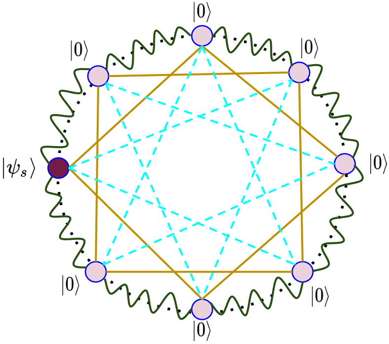
Figure 1: Circular waveguide setup for the generation of genuine multimode entanglement between eight optical modes. The dark circle represents the mode in which the squeezed state $|\psi_{s}\rangle$ is given as input, whereas the light circles denote the vacuum $|0\rangle$ modes. The dark green curved lines correspond to the nearest-neighbor (NN) interaction. Long-range interactions are shown as follows: next-nearest-neighbor (NNN) with light yellow straight lines and next-to-next-nearest-neighbor (NNNN) interaction as very light dashed blue lines. For a waveguide with a large number of modes, higher levels of long-range interaction has be incorporated. The interaction strengths of the NN and long-range interactions, in general, can be different.

Let us first introduce the model which describes the evolution of the product input state to a genuinely entangled multimode state. The system comprises $N$ identical waveguides arranged in a circular configuration and coupled to each other, with varying interaction strength (for a schematic description of the system, see Fig. 1 for $N=8$). The Hamiltonian that governs the interactions of the $N$ modes within the system is represented by

$$\begin{split}\hat{H}=&\sum_{i=1}^{[\frac{N}{2}]-1}\hbar J^{\prime}_{i}\sum_{j=1}^{N}(\hat{a}^{\dagger}_{j}\hat{a}_{j+i}+H.c.)+\\ &\frac{1}{1+\frac{1}{2}(1+(-1)^{N})}\hbar J^{\prime}_{[\frac{N}{2}]}\sum_{j=1}^{N}(\hat{a}^{\dagger}_{j}\hat{a}_{j+[\frac{N}{2}]}+\text{H.c.}),\end{split}$$ (1)

where an increasing $i$ indicates an increasing range of interactions. Here $N+j\equiv j(mod~{}N)$, $\hat{a}_{j}$ and $\hat{a}_{j}^{\dagger}$ are the bosonic annihilation and creation operators respectively, corresponding to the $j$-th mode, H.c. stands for the Hermitian conjugate, $J^{\prime}_{i}$ denotes interaction strength or coupling constants between waveguide modes with $J^{\prime}_{1}=J^{\prime}$ and $J^{\prime}_{i}=n_{i}J^{\prime}$ for $i\geq 2$ and we consider $\hbar=1$. Thus $J^{\prime}$ represents the strength of the nearest-neighbor (NN) coupling. The long-range interaction is introduced by making $n_{i}>0$ for $i\geq 2$. We must note that $n_{i}\neq 0$, if and only if $n_{j}\neq 0$ $\forall j<i$, with the condition $0<n_{i}\leq 2$ Dreisow et al. (2008). The second term in Eq. (1) takes care of the longest range of interactions between modes.

Note $\mathbf{1}$. The time evolution operator corresponding to the Hamiltonian in Eq. (1) is given by $\exp(-i\hat{H}t)$. Therefore, upon evolution, the final state of the waveguide system contains terms of the form $J^{\prime}t$. We relabel such parameters as $J$, representing the interaction strength or the coupling parameter and the range of the interactions is tuned with $n_{i}$. Thus, the variation with respect to $J$ also represents the variation in time. Moreover, note that $t=z\mu/c$, where $\mu$ is the refractive index for the waveguide mode, which relates the time duration $t$ to the propagation distance $z$. In order to create a genuine multimode entangled state from a fully product state, we study the dynamics induced by the aforementioned interactions to identify the optimal configuration of the waveguide system. In particular, one of the modes, say, the first mode, is chosen to be a single-mode squeezed state, $\ket{\psi_{\text{s}}}=\exp(\frac{1}{2}(\xi^{*}\hat{a}_{j}^{2}-\xi\hat{a}_{j}^{\dagger^{2}}))\ket{0}$ with $j$ being the input site, the squeezing parameter is $\xi=se^{i\theta}$, where $s$ is the squeezing strength and $\theta$ represents the squeezing angle. The rest of the modes are in the vacuum state, $|0\rangle$, i.e., the $N$-mode initial state takes the form as

$$|\psi\rangle_{\text{in}}=\ket{\psi_{\text{s}}}\otimes|0\rangle^{\otimes N-1}.$$ (2)

The covariance matrix corresponding to the above initial state has the form,

$$\Xi_{i}=\!\!\!\!\! \frac{1}{2}\Bigg{[}\begin{pmatrix}\cosh 2s+\cos\theta\sinh 2s&\sin\theta\sinh 2s\\ \sin\theta\sinh 2s&\cosh 2s-\cos\theta\sinh 2s\end{pmatrix}$$ (3)

$$\oplus\mathbb{I}^{\oplus N-1}\Bigg{]},$$

where $\mathbb{I}=\text{diag}(1,1)$ is the $2\times 2$ identity matrix. Note that due to the periodicity present in the model, the position of the mode in which the input squeezed state is taken cannot alter the multimode entanglement content of the final state.

The symplectic formalism is used to analyze the evolution of the Gaussian input state and to characterize its entanglement (see Appendix A for details of the analytical formalism). The covariance matrix corresponding to the initial state of the system is denoted as $\Xi_{\text{in}}$. The final state of the system, upon evolution, is characterized by ${\Xi_{f}}=S_{H}{\Xi_{in}}S_{H}^{T}$, where $S_{H}$ is the symplectic transformation of the waveguide Hamiltonian, as defined in Appendix A, for which the generalized geometric measure is computed (see Appendix. B for the computation of GGM for a pure CV Gaussian state). In Appendix C, we present the simplest model involving a state with three modes propagating through circularly coupled waveguide modes that have only the nearest-neighbor interaction. It is important to emphasize here that such treatment provides the possibility to address this problem involving an arbitrary number of modes.

Remark $\mathbf{1}$. Instead of the squeezed state, if one considers a coherent state as the input, such a generation of multimode entanglement is not possible. This can be explained by considering the covariance matrix of the coherent state, which is nothing but $\frac{1}{2}\mathbb{I}$. Thus, in this scenario, the input covariance matrix reduces to $\Xi_{i}=\frac{1}{2}\mathbb{I}^{\oplus N}$ and the final state of the system is denoted by a covariance matrix proportional to the identity matrix (since, $S_{H}S_{H}^{T}=\mathbb{I}^{\oplus N}$). Thus, starting from a product state, we again end up with a product state after evolution and the entanglement generation cannot occur.

Remark $\mathbf{2}$. With a squeezed coherent state as input in one of the modes (and vacuum in the rest) of Eq. (2), the entanglement generated among the $N$-modes is the same as that obtained via an input squeezed state.

III Advantage of long-range interaction in Entanglement creation

In typical waveguide systems studied in the literature, only the NN interactions are considered, while higher-order couplings lead to bosonic Hamiltonians with LR interactions as in Eq. (1) which will be the main focus of this work. The motivation behind such consideration is the fact that in several physical systems, especially quantum spin models, LR interactions have been shown to typically create highly multimode entangled states, which serve as resources for quantum information processing tasks.

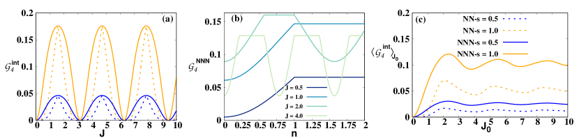
Figure 2: Generation of genuine multimode entanglement in a four-mode circularly coupled waveguide setup. (a). Variation of GGM, $\mathcal{G}_{4}^{\text{int}}$ (ordinate) against the coupling strength $J$ (abscissa) for nearest-neighbor (dashed line) and next-nearest-neighbor along with NN (solid lines) coupling. The squeezing strength of the initial state is taken to be $s=0.5$ (dark (blue)) and $s=1.0$ (light (orange)). (b). $\mathcal{G}_{4}^{\text{NNN}}$ (ordinate) is plotted with the variation of the strength of NNN coupling, $n$ (abscissa). Here the increase of $J$ ($J=0.5$, $J=1.0$, $J=2.0$, and $J=4.0$) is represented from dark to light lines. The initial squeezing strength is set to $s=1.0$. (c). The accumulated GGM, $\langle\mathcal{G}_{4}^{\text{int}}\rangle_{J_{0}}$ (ordinate) vs $J_{0}$ (abscissa) with similar specifications as in (a). All axes are dimensionless.

Before going into the results concerning circular waveguides with an arbitrary number of modes, let us first investigate the situation involving a small number of modes. Such analysis can also illustrate the benefit of LR interactions for producing genuine multimode entanglement (quantified by the generalized geometric measure), with the addition of higher-order couplings one by one.

III.1 Circular waveguide with four modes

Let us consider a four-mode circular arrangement of waveguides, where, in addition to the NN interaction, the next-nearest-neighbor (NNN) interaction is also introduced. Before considering the situation with both NN and NNN interactions, let us first concentrate on the dynamics of multimode entanglement in the model with only NN interaction.

III.1.1 Waveguide with nearest-neighbor interactions

Let us consider the Hamiltonian for the four-mode waveguide system given in Eq. (1) with $N=4$ by setting $n_{i}=0$ (for $i\geq 2$) which simulates only the NN interactions. By taking the initial state of the system as $\ket{\psi_{s}}\bigotimes\ket{0}^{\otimes 3}$, whose corresponding covariance matrix is given by Eq. (3), the GGM is determined by finding the symplectic eigenvalues of the reduced covariance matrices - (i) single mode: $\Xi_{f}^{i}$ with $i=1,\dots,4$ and (ii) two-mode: $\Xi_{f}^{1j}$ with $2\leq j\leq 4$. It is observed that for each such reduced covariance matrix, there is only one symplectic eigenvalue which is not equal to $1/2$. We represent such symplectic eigenvalues of the bipartitions as $\mathbf{v}=\{\nu_{i},\dots,\nu_{1j},\dots\}$. Therefore, the GGM reduces to

$$\mathcal{G}_{4}^{\text{int}}=\mathcal{G}_{4}^{\text{NN}}=1-\max_{\mathbf{v}}\Big{[}\frac{2}{1+2\nu_{k}}\Big{]},$$ (4)

where the superscript, int, represents the maximum LR interaction considered, while the subscript is for the total number of modes, and $k$ runs over the elements of the set $\mathbf{v}$.

Notice first that the above formalism holds for any number of modes and range of interactions (e.g., NN, NNN, etc.) as we will show in the succeeding section.

In the four-mode scenario, we find that the GGM is not affected by the squeezing angle, $\theta$. Additionally, as the squeezing strength increases, so does the GGM, and it is periodic with respect to $J$, with the period being $\pi$ (see Fig. 2 (a)). In this scenario, it is important to note that the $\nu_{k}$ values are dependent on both $J$ and $s$.

III.1.2 Model with next-nearest-neighbor interactions

The Hamiltonian for simulating both the NN and the NNN interaction in a four-waveguide system can be obtained from Eq. (1) by setting $N=4$, $J_{1}=J$, and $J_{2}=n_{2}J_{1}=nJ$. The method for calculating the GGM is similar to that for the nearest-neighbor case and it is dependent on $s$, $J$, and $n$. The strength of the next nearest-neighbor interaction can be greater than ($n>1$), or equal to ($n=1$), or less than ($n<1$) that of the NN interaction. Let us now analyze the behavior of the genuine multimode entanglement with time and compare it with the scenario involving only NN interactions. To study it, we compute $\mathcal{G}_{4}^{\text{NNN}}$. The juxtaposition of $\mathcal{G}_{4}^{\text{NN}}$ and $\mathcal{G}_{4}^{\text{NNN}}$ reveals the following facts:

1. Like with NN interactions, $\mathcal{G}_{4}^{\text{NNN}}$ increases with $s$ and is $\pi$-periodic with $J$.

2. On the other hand, with non-vanishing $n$, we find that $\mathcal{G}_{4}^{\text{NNN}}\geq\mathcal{G}_{4}^{\text{NN}}$ for a fixed value of $J$, although they coincide at the point where both of them reach their maximum as well as when they both are minimum.

3. Furthermore, the difference $(\mathcal{G}_{4}^{\text{NNN}}-\mathcal{G}_{4}^{\text{NN}})$ becomes maximum irrespective of $J$ when $n=1$, i.e., when the strength of the NNN interaction coincides with that of the NN case (see Fig. 2(b)). In other words, the enhancement of genuine multimode entanglement through LR over NN interaction is more pronounced when all the modes interact with each other equally.

III.2 Accumulated GGM

The question that naturally arises from the observations of systems having NN and NNN interaction is, how to manifest the beneficial role of LR interactions from the pattern of the GGM. Towards that aim, we introduce a figure of merit which we call accumulated GGM (AcGGM), defined as the area under the GGM curve over a given range of the coupling constant $J$. It can be interpreted as the entanglement assembled among the modes, during a particular time interval when the interaction is switched on. Mathematically, AcGGM can be defined as

$$\langle\mathcal{G}_{N}^{\text{int}}\rangle_{J_{0}}=\frac{1}{J_{0}}\int_{J=0}^{J_{0}}\mathcal{G}_{N}^{\text{int}}dJ,$$ (5)

where $J_{0}$ is the interval of $J$ over which the area under the GGM curve is calculated. The higher the value of $\langle\mathcal{G}_{N}^{\text{int}}\rangle_{J_{0}}$, the better the arrangement for creating genuine multimode entanglement within that range of $J$.

III.2.1 Accumulated GGM highlighting the power of LR interactions

We now focus on the impact of LR interactions on AcGGM. A few prominent features emerge –

• Input squeezing: For a given type of interaction, $\langle\mathcal{G}_{N}^{\text{int}}\rangle_{J_{0}}$ increases with the increase in the input squeezing strength $s$.

• LR interaction: For a given $s$, we clearly observe that $\langle\mathcal{G}_{N}^{\text{NNN}}\rangle_{J_{0}}>\langle\mathcal{G}_{N}^{\text{NN}}\rangle_{J_{0}}$ (see Fig. 2 (c)).

• Interaction strength: Another interesting aspect arises - although the GGM collapses and revives with $J$, AcGGM for a reasonably high $J_{0}$ value can be obtained without significant fluctuations.

Note $\mathbf{2}$. Five-mode circular waveguide system - The GGM for the five-mode waveguide exhibits qualitatively similar properties to $\mathcal{G}_{4}^{\text{int}}$. By taking the same kind of initial state, i.e., by choosing $|\psi_{s}\rangle\otimes|0\rangle^{\otimes 4}$, which evolves according to $\hat{H}$ in Eq. (1) with $J_{1}=J_{2}=J$, no periodicity in GGM with $J$ is observed for the nearest-neighbor case, while $\mathcal{G}^{\text{NNN}}_{5}$ exhibits a period of $\frac{4\pi}{5}$. Similar to the case of the four-mode waveguide, the NNN interaction, with strength equal to that of NN, furnishes a higher AcGGM as compared to the case with only nearest-neighbor coupling.

III.3 Six-mode circular waveguide

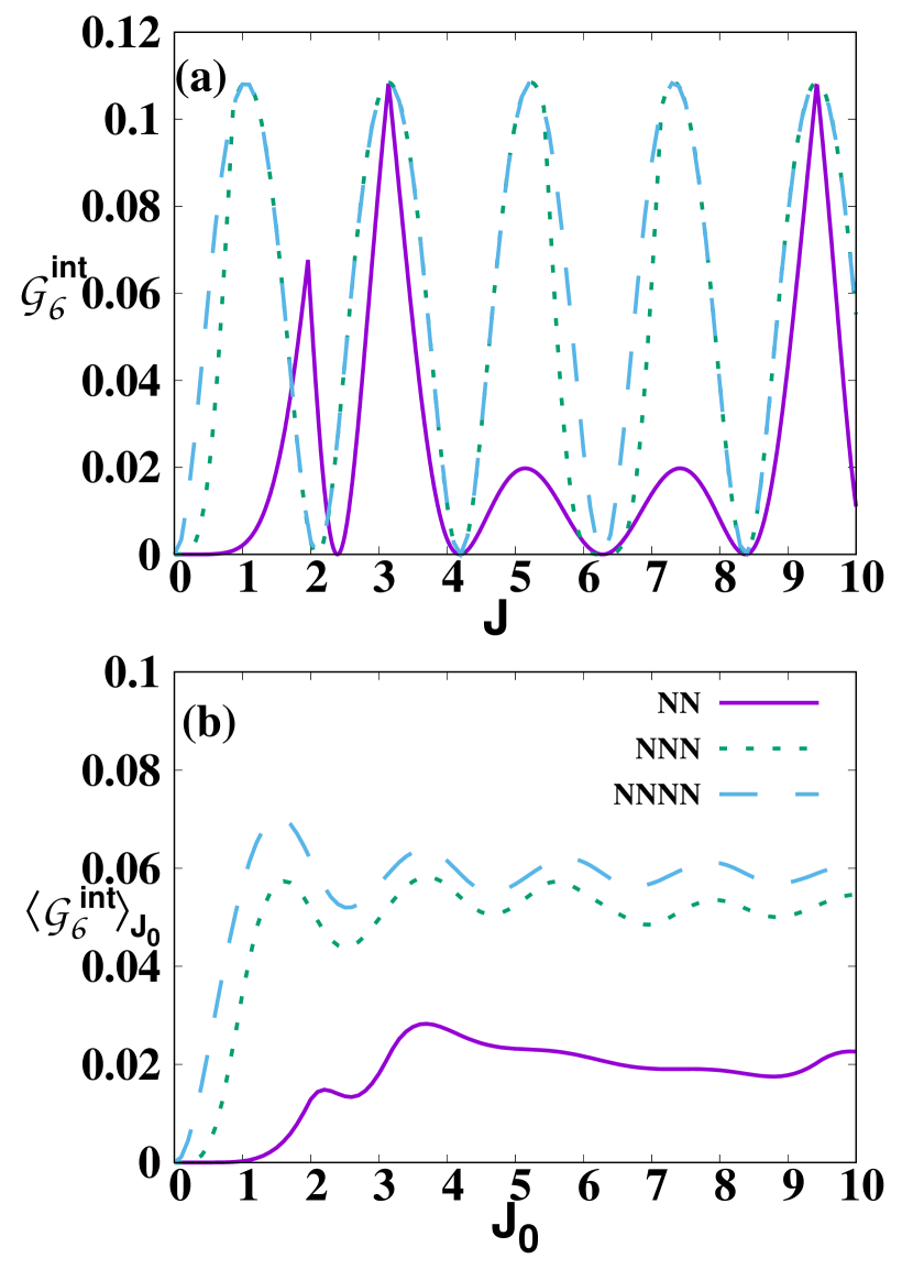
Figure 3: Circularly coupled waveguide involving $6$-modes. (Upper panel (a).) The genuine six-mode entanglement $\mathcal{G}_{6}^{\text{int}}$ (ordinate) against the coupling strength $J$ (abscissa) for $s=1.0$ comprising NN interaction ((purple) solid line), NNN interaction ((green) dotted line) and NNNN interaction ((blue) dashed line) having equal interaction strength. (Lower panel (b)). The variation of the accumulated GGM $\langle\mathcal{G}_{6}^{\text{int}}\rangle_{J_{0}}$ (ordinate) vs $J_{0}$ (abscissa). All other specifications are the same as in (a). All axes are dimensionless.

We now proceed to carry out the investigation when the waveguide arrangement comprises six modes, thereby incorporating a higher level of long-range interaction like the next-to-next-nearest-neighbor (NNNN) interaction. It is interesting to find out whether LR interactions are indeed responsible for creating genuine multimode entanglement even in the presence of weak coupling strengths. The Hamiltonian for the evolution, in this case, can be realized according to Eq. (1) with $N=6$ and $J_{1}=J$, $J_{2}=J_{1}=J$ and $J_{3}=n_{3}J_{1}=nJ$, where the same strength of interaction for NN and NNN couplings is considered based on the observations for the four-mode waveguides. Interestingly, the maximum GGM in the NNNN interaction case is again obtained when the coupling strength is equal to that of the short-range interactions, NN and NNN. Again the GGM oscillates with $J$, irrespective of short- and long-range interactions, although, unlike the four-mode scenario, the pattern of the GGM changes with the introduction of LR interactions. In particular, the GGM vanishes with NNNN and NNN interactions when $J$ is a multiple of $\frac{4\pi}{6}$, which is not the case for NN interactions and the maximal value of the GGM is obtained more frequently with respect to $J$ in the presence of both LR interactions as compared to that of the NN interaction. Akin to the four- and five-mode waveguide scenarios, $\mathcal{G}_{6}^{\text{NNNN}}\geq\mathcal{G}_{6}^{\text{NNN}}\geq\mathcal{G}_{6}^{\text{NN}}$ (see Fig. 3 (a)), although the maximum value of the GGM cannot be increased by the LR interactions for a fixed $J$ value. Quantitatively, this feature can be captured by considering the AcGGM, i.e., $\langle\mathcal{G}_{6}^{\text{NNNN}}\rangle_{J_{0}}>\langle\mathcal{G}_{6}^{\text{NNN}}\rangle_{J_{0}}>\langle\mathcal{G}_{6}^{\text{NN}}\rangle_{J_{0}}$ as depicted in Fig. 3 (b). We observe that LR interactions with low coupling strength can indeed create more GGM than in the NN case, as is illustrated in Fig. 3 (a). for $0\leq J\leq 1$.

The results of circular waveguide setups with four-, five-, and six-modes strongly indicate that incorporating long-range interactions is beneficial and that the same interaction strength for all kinds of coupling provides the best genuine multimode entanglement.

III.4 GME produced with $N$-mode circular waveguide

Motivated by the results obtained in the previous subsections, we compute the production of genuine multimode entanglement in arbitrary modes, say, $N$-modes arranged in a circle. The Hamiltonian for the same pertains to an $N$-mode circularly coupled waveguide system, with its input state being specified by $\ket{\psi}_{in}^{12\cdots N}=\ket{\psi_{s}}\otimes\ket{0}^{\otimes N-1}$. Since the studies in the previous subsections display the preferable role of equal short- and long-range interaction strengths, we take all the modes to be interacting equally with each other. Moreover, this configuration produces the maximum amount of AcGGM, as discussed beforehand.

Let us analyze the dynamics of GGM in this situation. Since the definition of GGM involves the Schmidt coefficients in an arbitrary number of bipartitions, the computation of GGM is hard for systems involving an arbitrary number of modes, unless some symmetry present in the system is identified. Previous configurations with four-, five-, and six-modes indicate that there is a symmetry under permutation of the modes in the evolved state, $\ket{\psi}_{f}^{12\cdots N}$, due to the circular configuration. As a consequence of this symmetry, there is only $(N-1)$ number of different bipartitions that require to be considered. For an even number of modes i.e., $N=2m$, the contributing bipartitions, pertaining to a given number of submodes, can be divided into two sets - one set which involves the mode in which the squeezed input state is taken, and another set that does not include the mode with the squeezed input state. Without loss of generality, if we start with a state in which the input state is plugged in the first mode, the bipartitions among the modes under study are $1:\text{rest}$, $2:\text{rest}$, $12:\text{rest}$, $23:\text{rest}$, $\cdots$, $12\dots[N/2]-1:\text{rest}$, $23\dots[N/2]:\text{rest}$ and $12\dots[N/2]:\text{rest}$, while if $N=2m+1$, we must consider $23\dots[N/2]+1:\text{rest}$, as an additional bipartition (here $``\text{rest}"$ in $i:\text{rest}$ denotes all the modes except $i$). We observe that the largest symplectic eigenvalue in $2:\text{rest}$ bipartition ultimately leads to the GGM, given by

$$\nu=\frac{\sqrt{\frac{1}{4}f_{1}(N)-2\sinh^{2}s\left[f_{2}(N)\cos\left(\frac{JN}{2}\right)+\cos\left(JN\right)\right]+f_{3}(N)\cosh 2s}}{N^{2}},$$ (6)

where $f_{1}(N)=\left(N^{4}-4N^{2}+12\right)$, $f_{2}(N)=\left(N^{2}-4\right)$, and $f_{3}(N)=\left(N^{2}-3\right)$. The expression of the GGM then takes the form as

$$\mathcal{G}^{LR}_{N}=1-\frac{2}{2\nu+1},~{}~{}~{}~{}~{}~{}~{}\text{for}~{}~{}N\geq 4.$$ (7)

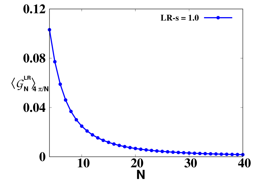
Figure 4: Accumulated GGM, $\langle{\mathcal{G}^{LR}_{N}}\rangle_{\frac{4\pi}{N}}$ (ordinate) against the number of modes $N$ (abscissa), when long-range interaction among all the modes with equal coupling strength is applied. The integration is performed a period of $\frac{4\pi}{N}$ Here $s=1.0$, the squeezing parameter of the initial state, $\ket{\psi_{s}}\otimes\ket{0}^{\otimes N-1}$. Both axes are dimensionless.

It can be easily seen that $\mathcal{G}^{LR}_{N}$ is a periodic function of $J$ with a period of $\frac{4\pi}{N}$. Hence, we calculate the accumulated GGM over a period, defined in Eq. (5) with $J_{0}=\frac{4\pi}{N}$, to see how it behaves with an increasing number of modes. $\langle{\mathcal{G}^{LR}_{N}}\rangle_{\frac{4\pi}{N}}$ decreases monotonically with an increasing $N$ at a fixed initial squeezing strength as shown in Fig. 4 with $s=1.0$. This indicates that for a given initial squeezing strength of the input mode, creating genuine multimode entanglement becomes more difficult with an increase in the number of interacting modes. Moreover, the maximum $\mathcal{G}^{LR}_{N}$ achievable also decreases monotonically with increasing modes. Both the results demonstrate that there is a trade-off between the increment in the number of modes and the LR interactions involved during the dynamics.

IV Creation of constant GGM in waveguides with disorder

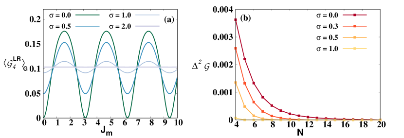
Figure 5: Quenched averaged genuine multimode entanglement in circular waveguides coupled with disordered interaction strength. (a). The variation of the four-mode quenched GGM, $\langle\mathcal{G}^{LR}_{4}\rangle_{G}$, (ordinate) with respect to the mean coupling strength $J_{m}$ (ordinate). Dark to light lines represents $\sigma=0.0,0.5,1.0,$ and $2.0$ respectively. (b). The breached GGM, $\Delta^{2}\mathcal{G}$, given in Eq. (9) (ordinate) with the number of modes, $N$ (abscissa). Again, dark to light lines represents $\sigma=0.1,0.3,0.5$ and $1.0$ respectively. All axes are dimensionless.

Due to the periodic nature of multimode entanglement as described in the preceding section, the method can be argued to have a limitation. In particular, since it collapses and revives with the variation of the interaction strength $J$, we may end up with almost vanishing entanglement among the modes for certain values of $J$. Note that, since $J$ contains an implicit factor of time ($t$), this implies that the genuine multimode entanglement fluctuates with time, thereby creating entanglement that can be used only at certain instants. A natural question at this point is how one can circumvent this feature. We indeed show that a stable (fluctuation-free) multimode entangled state can be produced when the system has some imperfections. Given the experimental challenges in implementing interactions of a fixed strength, it is quite natural to consider that $J$ does not remain constant but fluctuates around the desired value. Typically, the disorder in system parameters is responsible for the detrimental effect on the system properties, although there are certain instances in which imperfections can enhance physical characteristics Aharony (1978); Feldman (1998); Abanin et al. (2007); Niederberger et al. (2008); Prabhu et al. (2011); Sadhukhan et al. (2015); Mishra et al. (2016); Sadhukhan et al. (2016) like magnetization and entanglement in the modes Bera et al. (2016, 2017); Mishra et al. (2016). We will illustrate here other aspects of the disordered model.

To simulate such behavior, we consider a disordered model, in which $J$ comes from a Gaussian distribution of mean $J_{m}$ and standard deviation $\sigma$. Here, $J_{m}$ is the desired interaction strength to be tuned, and a higher $\sigma$ indicates a larger fluctuation around the value $J_{m}$, thereby measuring the strength of the disorder. We assume that the time scale taken by the disordered interaction strength to attain its equilibrium value is much larger than the implementation time, which allows us to define the quenched average GGM over the Gaussian distribution as

$$\langle{\mathcal{G}^{LR}_{N}}\rangle_{G}=\frac{1}{\sqrt{2\pi}\sigma}\int_{-\infty}^{+\infty}\mathcal{G}^{LR}_{N}~{}\exp(-\frac{(J-J_{m})^{2}}{2\sigma^{2}})~{}dJ.$$

It is observed that $\langle\mathcal{G}^{LR}_{N}\rangle_{G}$ fluctuates with respect to $J_{m}$ with the same period $4\pi/N$, albeit the amplitude of the fluctuations decreases with increasing $\sigma$, as shown for a four-mode disordered waveguide setup in Fig. 5(a). For high enough standard deviation, e.g., $\sigma\geq 2$, the entanglement fluctuation is negligible and an almost constant value is present over the entire range of $J_{m}$. Therefore, our findings manifest that although $\langle\mathcal{G}_{N}^{LR}\rangle_{G}$ decreases in comparison to the maximum GGM achieved in the ordered model, a constant GGM with lower fluctuations can only be obtained when the evolution occurs according to the disordered model.

IV.1 Quantification of disorder rendered GGM stability

As defined in Sec. III.2, we can define the quenched average accumulated GGM as

$$\langle\langle{\mathcal{G}^{LR}_{N}}\rangle_{G}\rangle_{J_{m0}}=\frac{N}{4\pi}\int_{0}^{J_{m0}}\langle{\mathcal{G}^{LR}_{N}}\rangle_{G}~{}dJ_{m}$$

in order to investigate the effect of the disorder. This can be interpreted as the area under the quenched average GGM curve. From Fig. 5 (a), it is clear that the mean value of $\langle\mathcal{G}_{N}^{LR}\rangle_{G}$ over a cycle remains constant with the variation of $\sigma$. Thus although the amplitude changes, $\langle\langle{\mathcal{G}^{LR}_{N}}\rangle_{G}\rangle_{J_{m0}=4\pi/N}$ does not vary with the strength of the disorder, $\sigma$. Hence,

$$\langle\langle{\mathcal{G}^{LR}_{N}}\rangle_{G}\rangle_{4\pi/N}=\langle\mathcal{G}_{N}^{LR}\rangle_{4\pi/N},$$ (8)

which means, even after the introduction of disorder, the value of GGM, on average over the coupling strength (or, time $t$), remains unchanged. Indeed, the GME content is now dispersed more consistently throughout the evolution time. Furthermore, it is observed that the constructive effect of long-range interactions persists even in the presence of disorder, which implies that the Hamiltonian comprising all interacting modes with equal strength, provides a much higher quenched average GGM than that with NN interactions. The decreasing fluctuations in the quenched average GGM can be quantified by the standard deviation of $\langle\mathcal{G}^{LR}_{N}\rangle_{G}$, which is defined as

$$\Delta^{2}\mathcal{G}=\langle\langle\mathcal{G}^{LR}_{N}\rangle_{G}^{2}\rangle_{4\pi/N}-\langle\langle{\mathcal{G}^{LR}_{N}}\rangle_{G}\rangle_{4\pi/N}^{2},$$ (9)

where the average is taken with respect to $J_{m}$ over a full cycle. We call this quantity as the breached GGM, whose low value implies the generation of stable quenched genuine multimode entanglement. We find that this is indeed the case, i.e., the presence of disorder reduces the fluctuations in the quenched average accumulated GGM. Moreover, $\Delta^{2}\mathcal{G}$ decreases with the increase of $N$, as illustrated in Fig. 5 (b). Our studies demonstrate that the oscillations in the quenched average GGM disappear with the increase of the disorder strength and the number of modes, although the increase of the system size has a destructive effect on the creation of GGM like the ordered system.

V Block entanglement entropy

We have already established that the genuine multimode entanglement content can be enhanced with the addition of LR interactions. Instead of quantifying the multimode entanglement geometrically, let us study the entanglement production in bipartitions, i.e., we compare the block entropy of entanglement produced through dynamics with the nearest-neighbor interaction as well as with the long-range interactions. In particular, we look into the scaling of the entropy Wehrl (1978) for the reduced density matrices of the final state, $\ket{\psi}_{f}^{12...N}$, with respect to the number of subsystems comprising the reduced state. Note that we need to consider $[N/2]-1$ number of reduced density matrices for an $N$-mode system which are $\rho_{2}$, $\rho_{23}$, …, $\rho_{23...[N/2]}$ where $\rho_{23...i}=\tr_{1,i+1,...N}\ket{\psi}_{f}^{12...N}\bra{\psi}_{f}^{12...N}$. For a fixed system size, we compute the Renyi-$2$ block entropy defined as $S(\rho_{L})=-\ln[\Tr(\rho_{L}^{2})]$ Renyi (1960); Nielsen and Chuang (2010) by varying the block size $L$, where $\rho_{L}=\Tr_{\bar{L}}|\psi\rangle_{f}^{12...N}\langle\psi|_{f}^{12...N}$, with $\bar{L}$ being the rest of the modes which are not included in the block, $L$. In the covariance matrix formalism, it can be simplified to $S(\rho)=\frac{1}{2}\ln(2^{2L}\det\Xi_{L})$ where $\det\Xi_{L}$ is the determinant of the covariance matrix corresponding to an $L$-mode state $\rho_{23...L}$ Adesso et al. (2014).

In the case of NN interaction (see Fig. 6(a)), it can be observed that $S(\rho_{L})$ increases steadily with $L$ for a while, and then saturates with $L$ which increases with $J$. Moreover, the saturation value of $S(\rho_{L})$ is the same for all interaction strengths with $J>1$ whereas when $J\leq 1$, the block entanglement entropy saturates to different values, which again increases with $J$.

On the other hand, for long-range interactions with all interaction strengths being equal, as depicted in Fig. 6(b), $S(\rho_{L})$ always increases monotonically with $L$, and the behavior of the block entropy does not follow any order with respect to $J$, contrary to the NN-interaction regime. We recall that $2^{2L}\det\Xi_{L}=1$ for a pure Gaussian state while it is greater than unity for a Gaussian mixed state. Thus, in the case of LR interactions, the increase in $S(\rho_{L})$ indicates that the reduced subsystems involving a larger number of modes tend towards more mixed states. It has also been established that the symplectic eigenvalues of pure Gaussian states are all equal to $1/2$ while they are greater for mixed states Adesso et al. (2014). Since the reduced subsystems of larger length have less purity, the symplectic eigenvalues of the single-mode reduced state contribute to the GGM (since we take the maximum of $\frac{2}{1+2\nu}$) as shown in Sec. III.4, thereby shedding light on the computation of GGM.

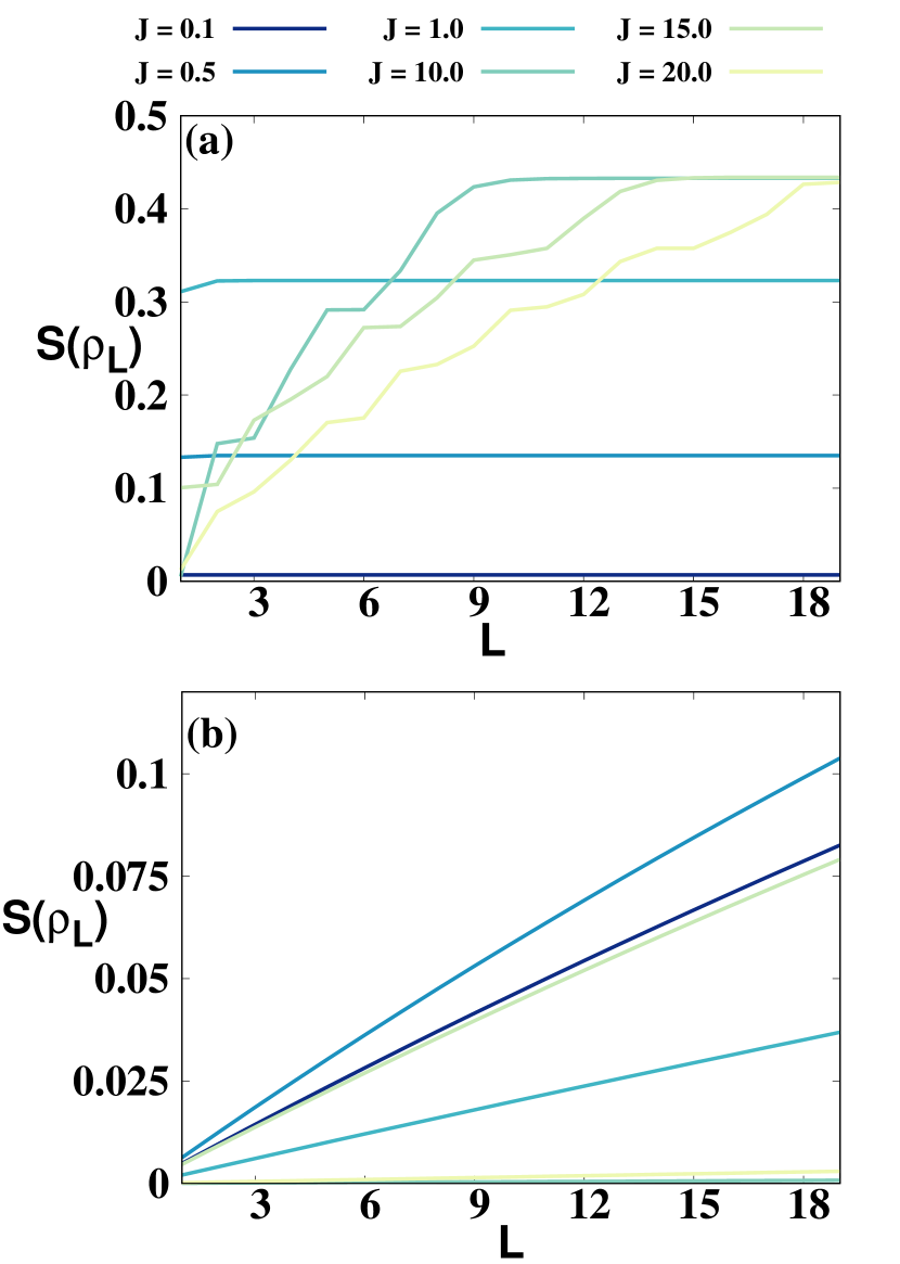
Figure 6: Block entanglement entropy, $S(\rho_{L})$ vs the reduced system size, $L$, when the initial squeezing strength is fixed to $s=1.0$. (a). The interaction is considered to be nearest-neighbor (NN) while in (b), interactions among all the modes are long range. Here $N=40$, i.e., $40$ circularly waveguide modes are coupled. From dark to light, the lines represent $J=0.1$, $J=0.5$, $J=1.0$, $J=10.0$, $J=15.0$, and $J=20.0$ respectively. All axes are dimensionless.

VI Conclusion

Entangled continuous variable (CV) systems are of fundamental importance in realizing a host of quantum information protocols. Additionally, it has been demonstrated that entangled CV systems provide a key route for resolving issues with other photonic devices, such as challenges with Bell-state measurements. Therefore, designing a scheme to generate multimode-entangled states is of paramount interest.

We demonstrated that multiple circularly coupled interacting optical waveguide modes have the potential to create highly genuine multimode-entangled states. Specifically, the interacting circular waveguide can create a genuinely multimode entangled (GME) state, measured by using generalized geometric measure (GGM), from a squeezed or squeezed coherent state in a single mode that is a product with vacuum states in the other modes. We point out that we have considered an experimentally feasible configuration for our study. The waveguide arrays proposed in this work can be fabricated using direct femto-second laser inscription. Waveguide configurations are appropriate because, unlike bulk optical elements, the propagation losses in these systems can be quite low. Additionally, the parametric down-conversion process can be used to generate the squeezed state that we have considered as the input.

We analyzed the impact of different ranges of interaction on the generation of a GME state from the product initial state. We illustrated how the incorporation of long-range interactions constructively affects the process. Specifically, long-range interactions help in generating higher genuine entanglement for a fixed strength of coupling constant, compared to the circular waveguide setup with only nearest-neighbor interaction, even though the maximum value of the GGM remains constant for both long-range and nearest-neighbor interactions. When the order of the long-range interaction is such that all the modes interact equally with each other, we analytically found the GGM, which varies periodically with the coupling strength. We noticed that the GGM content can be increased with an increase of the squeezing strength in the input modes. To access the benefit of LR interactions quantitatively, we investigated the area under the GGM curve, which clearly furnishes a higher value for LR interactions, than that for waveguide modes coupled with short-range couplings. We noted, however, that the genuine multimode entanglement generated decreases with an increase in the number of interacting modes, thereby indicating a complementary relation with system size and range of interactions.

One of the drawbacks of generating multimode entanglement via such a setup is that its magnitude fluctuates with time and thus is unsuitable for utilization in protocols that require states with a certain value of entanglement. To circumvent this unwanted characteristic, we showed that the presence of disorder in coupling between modes of waveguides can be useful. Starting from a product state, when the system evolves according to the circular waveguide Hamiltonian in which mode-couplings are chosen randomly from a Gaussian distribution of a fixed mean and standard deviation, with a higher standard deviation representing greater disorder in the setup, we calculated the quenched average GGM. Our results indicated that for a sufficient strength of disorder, the multimode entanglement ceases to fluctuate and saturates to a fixed quenched average value. Although the quenched average GGM can never reach the maximum possible value, which can be achieved in the absence of disorder, its constant magnitude can help in its utilization in information processing tasks. In summary, our results of the disordered model used in the evolution operator are an addition to the generic physical systems, and possibly first in photonic waveguides, which report the beneficial effect of disorder for generating genuine multimode entanglement.

Apart from the generation of genuine multimode entanglement, we showed that such a process is able to create entanglement in each bipartition. With nearest-neighbor interactions of moderate strength, the block entanglement entropy increases with the increase of the block length, while in the case of long-range interactions, it decreases. The observation is also in good agreement with the way the GGM expression is obtained.

Looking at the possibility of realizing waveguide setups in laboratories, our method opens up the possibility to build quantum devices which require multimode entanglement. Although we have concentrated on photonic waveguides, our findings also apply to the coupled-cavity arrays and micro-ring resonator devices. Hartmann et al. (2006).

VII Acknowledgement

TA, AP, RG and ASD acknowledge the support from the Interdisciplinary Cyber-Physical Systems (ICPS) program of the Department of Science and Technology (DST), India, Grant No.: DST/ICPS/QuST/Theme- 1/2019/23. AR gratefully acknowledges a research grant from Science and Engineering Research Board (SERB), Department of Science and Technology (DST), Government of India (Grant No. CRG/2019/005749) during this work.

Appendix A Primer on CV-systems

A continuous variable system is characterized by quadrature variables, such as $\hat{X}$ and $\hat{P}$, which are canonically conjugate with each other Serafini (2017); Braunstein and van Loock (2005). Such observables possess an infinite spectrum and their eigenstates constitute the basis for the infinite-dimensional Hilbert space. For an $N$-mode system, the Hamiltonian comprises $2N$ parameters, $\{\hat{X}_{k},\hat{P}_{k}\}$ (with $k=1,2,\dots,N$), and is defined as

$$\hat{H}=\frac{1}{2}\sum_{k=1}^{N}(\hat{X}_{k}^{2}+\hat{P}_{k}^{2})=\sum_{k=1}^{N}\Big{(}\hat{a}_{k}^{\dagger}\hat{a}_{k}+\frac{1}{2}\Big{)},$$ (10)

where $\hat{a}_{k}^{\dagger}$ and $\hat{a}_{k}$ are the creation and annihilation operators respectively for the mode $k$ and are given in terms of the quadrature variables as

$$\hat{a}_{k}=\frac{\hat{X}_{k}+i\hat{P}_{k}}{\sqrt{2}},~{}~{}~{}~{}~{}~{}~{}\text{and}~{}~{}~{}~{}~{}~{}\hat{a}_{k}^{\dagger}=\frac{\hat{X}_{k}-i\hat{P}_{k}}{\sqrt{2}},$$ (11)

with $i=\sqrt{-1}$. The creation and annihilation operators corresponding to a given mode satisfy the bosonic commutation relation, $[\hat{a}_{k}^{\dagger},\hat{a}_{k}]=1$. We can define a quadrature vector, $\hat{R}=(\hat{X}_{1},\hat{P}_{1},\dots,\hat{X}_{N},\hat{P}_{N})^{T}$, to rewrite the commutation relation more succinctly as

$$\left[\hat{R}_{k},\hat{R}_{l}\right]=i\mathcal{M}_{kl}\quad\text{with}~{}~{}\mathcal{M}=\bigoplus\limits_{j=1}^{\mathcal{N}}\Omega_{j}.$$ (12)

Here, $\mathcal{M}$ represents the $\mathcal{N}$-mode symplectic form, and $\Omega_{j}$, for a single mode, is given by

$$\quad\Omega_{j}=\begin{pmatrix}0&1\\ -1&0\end{pmatrix}\forall j.$$ (13)

Out of the plethora of CV quantum states, Gaussian states constitute the most widely studied class of states Ferraro et al. (2005); Weedbrook et al. (2012). Such states are the ground and thermal states of Hamiltonians which are at most quadratic functions of the quadrature variables. As the name suggests, Gaussian states can be completely characterized by their first and second moments, encapsulated respectively by the displacement vector $\mathbb{d}$ and the covariance matrix $\Xi$, in the following way:

$$d_{k}=\expectationvalue{\hat{R}_{k}}_{\rho},$$ (14)

$$\Xi_{kl} =\frac{1}{2}\expectationvalue{\hat{R}_{k}\hat{R}_{l}+\hat{R}_{l}\hat{R}_{k}}_{\rho}-\expectationvalue{\hat{R}_{k}}_{\rho}\expectationvalue{\hat{R}_{l}}_{\rho}.$$ (15)

Here, $\rho$ denotes the $N$-mode Gaussian state under consideration and $\Xi$ is a real, symmetric, and positive definite $2N$ dimensional square matrix. Gaussian dynamics are similarly affected by second-order Hamiltonians. For analytical simplicity, we can resort to the symplectic formalism. Given any $N$-mode quadratic Hamiltonian $\hat{\mathcal{H}}$ which can be written as $\hat{\mathcal{H}}=\hat{\xi}^{\dagger}H\hat{\xi}$ with $\hat{\xi}=\left(\hat{a}_{1},\hat{a}_{2},...,\hat{a}_{N},\hat{a}_{1}^{\dagger},...,\hat{a}_{N}^{\dagger}\right)^{T}$, we can construct its corresponding symplectic matrix $S_{H}$ as Luis and Sanchez-Soto (1995); Arvind. et al. (1995); Adesso et al. (2014)

$$S_{H}=T^{\dagger}L^{\dagger}\exp{-iKH}LT,$$ (16)

where $K,L$ and $T$ are $2N\times 2N$ matrices given by

$$K=\begin{pmatrix}\mathbb{I}_{N}&\mathbb{O}_{N}\\ \mathbb{O}_{N}&-\mathbb{I}_{N}\end{pmatrix},$$ (17)

$$L=\frac{1}{\sqrt{2}}\begin{pmatrix}\mathbb{I}_{N}&i\mathbb{I}_{N}\\ \mathbb{I}_{N}&-i\mathbb{I}_{N}\end{pmatrix},$$ (18)

$$T_{jk}=\delta_{k,2j-1}+\delta_{k+2N,2j}.$$ (19)

Here, $\mathbb{I}_{N}$ is the $N$-dimensional identity and $\mathbb{O}_{N}$ is the null matrix. Thereafter, the evolution of the Gaussian state in terms of its displacement vector and covariance matrix is defined as Adesso et al. (2014)

$$\rho^{\prime}=e^{-i\hat{\mathcal{H}}t}\rho e^{i\hat{\mathcal{H}}t}\equiv \mathbb{d}^{\prime}=S_{H}\mathbb{d},$$ (21)

$$\Xi^{\prime}=S_{H}\Xi S_{H}^{T}.$$

Appendix B Genuine multimode entanglement for CV systems

In the discrete variable regime, a pure multipartite state, $|\psi\rangle_{1,2,\dots,N}$, is said to be genuinely entangled if it has a non-vanishing value of the generalized geometric measure (GGM) Shimony (1995); Barnum and Linden (2001) defined as follows

$$\mathbb{G}(|\psi\rangle_{1,2,\dots,N})=1-\max_{|\phi\rangle\in\mathcal{S}}|\langle\phi|\psi\rangle_{1,2,\dots,N}|^{2},$$ (22)

where $|\phi\rangle$ is an $N$-party pure state which is not genuinely entangled, and the Fubini Study metric is used as the distance measure Arnold (1978); Kobayashi and Nomizu (2009). A simpler canonical form of the GGM was derived Sen (De) which reads as

$$\mathbb{G}(|\psi\rangle_{1,2,\dots,N})=1-\max[\lambda_{A:B}|A\cup B =\{1,\dots,N\},$$

$$A\cap B=\varnothing],$$ (23)

where $\lambda_{A:B}$ is the maximum eigenvalue of the reduced density matrix in the $A:B$ split of the state $|\psi\rangle_{1,2,\dots,N}$. The maximization is performed over all such possible bipartitions.

In the case of pure CV Gaussian systems, the genuine multimode entanglement is quantified using a similar measure Roy et al. (2020), defined as

$$\mathcal{G}(|\psi\rangle_{1,2,\dots,N})=1-\max\mathcal{P}_{m}\Big{[}\prod_{i=1}^{m}\frac{2}{1+2\nu_{i}}\Big{]}_{m=1}^{[N/2]},$$ (24)

where $\mathcal{P}_{m}$ represents all the $m$-mode reduced states corresponding to the $N$-mode pure state $|\psi\rangle_{1,2,\dots,N}$ and $\nu_{i}$ stand for the symplectic eigenvalues of the $m$-th reduced state. The number of such bipartitions considered is $[N/2]$ with $[x]$ denoting the integer part of $x$.

Appendix C GGM for the three-mode waveguide

The simplest Hamiltonian corresponding to Eq. (1) is for the three-mode circular waveguide consisting of only nearest-neighbor (NN) interaction,

$$\hat{H}=\hbar J(\hat{a}_{1}^{\dagger}\hat{a}_{2}+\hat{a}_{2}^{\dagger}\hat{a}_{3}+\hat{a}_{3}^{\dagger}\hat{a}_{1}+H.c.),$$ (25)

where we have considered the interaction strength as $J_{1}=J$ and $\hbar=1$. The symplectic eigenvalues corresponding to the evolved three-mode input state, $|\psi\rangle_{\text{in}}=|\psi_{\text{s}}\rangle\otimes|0\rangle^{\otimes 2}$ are given by

$$\mathbf{v}_{1}=\left|\frac{1}{18}i\sqrt{16\sinh^{2}s\left(\cos\frac{3J}{2}+2\cos 3J\right)-24\cosh 2s-57}\right|,$$ (26)

$$\text{and}\,\,\mathbf{v}_{2}=\mathbf{v}_{3}=\left|\frac{1}{18}i\sqrt{8\sinh^{2}s\left(5\cos\frac{3hJ}{2}+\cos 3hJ\right)-24\cosh 2s-57}\right|,$$ (27)

where $\mathbf{v}_{i}$ represents the symplectic eigenvalue of the single-mode reduced states corresponding to the $i:jk$ bipartition (for $j,k\neq i$ and $i,j,k=1,2,3$). The GGM, in this case, exhibits periodic behavior with variation in $J$ at a period of $4\pi/3$. As the initial squeezing strength of the input state increases, so does the GGM. For $s=1.0$, $\mathcal{G}_{3}^{\max}\approx 0.2$ at $J\approx 1.4$. In this setup, no long-range interaction is possible due to the periodic nature of the waveguide Hamiltonian.

References

- Serafini (2017) A. Serafini, Quantum Continuous Variables, 1st ed. (CRC Press, 2017).
- Furusawa et al. (1998) A. Furusawa, J. L. Sørensen, S. L. Braunstein, C. A. Fuchs, H. J. Kimble, and E. S. Polzik, Science 282, 706 (1998).
- Bowen et al. (2003) W. P. Bowen, N. Treps, B. C. Buchler, R. Schnabel, T. C. Ralph, H.-A. Bachor, T. Symul, and P. K. Lam, Phys. Rev. A 67, 032302 (2003).
- Mizuno et al. (2005) J. Mizuno, K. Wakui, A. Furusawa, and M. Sasaki, Phys. Rev. A 71, 012304 (2005).
- Li et al. (2002) X. Li, Q. Pan, J. Jing, J. Zhang, C. Xie, and K. Peng, Phys. Rev. Lett. 88, 047904 (2002).
- Lance et al. (2005) A. M. Lance, T. Symul, V. Sharma, C. Weedbrook, T. C. Ralph, and P. K. Lam, Phys. Rev. Lett. 95, 180503 (2005).
- Andersen et al. (2005) U. L. Andersen, V. Josse, and G. Leuchs, Phys. Rev. Lett. 94, 240503 (2005).
- Yoshikawa et al. (2016) J. Yoshikawa, S. Yokoyama, T. Kaji, C. Sornphiphatphong, Y. Shiozawa, K. Makino, and A. Furusawa, APL Photonics 1, 060801 (2016).
- Raussendorf and Briegel (2001) R. Raussendorf and H. J. Briegel, Phys. Rev. Lett. 86, 5188 (2001).
- Horodecki et al. (2009) R. Horodecki, P. Horodecki, M. Horodecki, and K. Horodecki, Rev. Mod. Phys. 81, 865 (2009).
- Masada et al. (2015) G. Masada, K. Miyata, A. Politi, T. Hashimoto, J. L. O’Brien, and A. Furusawa, Nature Photonics 9, 316 (2015).
- Lenzini et al. (2018) F. Lenzini, J. Janousek, O. Thearle, M. Villa, B. Haylock, S. Kasture, L. Cui, H. Phan, D. V. Dao, H. Yonezawa, P. K. Lam, E. . H. Huntington, and M. Lobino, Science Advances 4, eaat9331 (2018).
- Larsen et al. (2019) M. V. Larsen, X. Guo, C. R. Breum, J. S. Neergaard-Nielsen, and U. L. Andersen, npj Quantum Information 5, 46 (2019).
- Simon (2000) R. Simon, Phys. Rev. Lett. 84, 2726 (2000).
- Duan et al. (2000) L.-M. Duan, G. Giedke, J. I. Cirac, and P. Zoller, Phys. Rev. Lett. 84, 2722 (2000).
- Giedke et al. (2001) G. Giedke, B. Kraus, M. Lewenstein, and J. I. Cirac, Phys. Rev. A 64, 052303 (2001).
- van Loock and Furusawa (2003) P. van Loock and A. Furusawa, Phys. Rev. A 67, 052315 (2003).
- Armstrong et al. (2015) S. Armstrong, M. Wang, R. Y. Teh, Q. Gong, Q. He, J. Janousek, H. Bachor, M. D. Reid, and P. K. Lam, Nature Physics 11, 167 (2015).
- Qin et al. (2019) Z. Qin, M. Gessner, Z. Ren, X. Deng, D. Han, W. Li, X. Su, A. Smerzi, and K. Peng, npj Quantum Information 5, 3 (2019).
- Adesso et al. (2004) G. Adesso, A. Serafini, and F. Illuminati, Phys. Rev. A 70, 022318 (2004).
- Braunstein and van Loock (2005) S. L. Braunstein and P. van Loock, Rev. Mod. Phys. 77, 513 (2005).
- Gühne and Tóth (2009) O. Gühne and G. Tóth, Physics Reports 474, 1 (2009).
- Takesue et al. (2008) H. Takesue, H. Fukuda, T. Tsuchizawa, T. Watanabe, K. Yamada, Y. Tokura, and S. Itabashi, Opt. Express 16, 5721 (2008).
- Camacho (2012) R. M. Camacho, Opt. Express 20, 21977 (2012).
- Das et al. (2017) S. Das, V. E. Elfving, S. Faez, and A. S. Sørensen, Phys. Rev. Lett. 118, 140501 (2017).
- Kannan et al. (2020) B. Kannan, D. L. Campbell, F. Vasconcelos, R. Winik, D. K. Kim, M. Kjaergaard, P. Krantz, A. Melville, B. M. Niedzielski, J. L. Yoder, T. P. Orlando, S. Gustavsson, and W. D. Oliver, Sci Adv 6 (2020), 10.1126/sciadv.abb8780.
- Zhang et al. (2021) Z. Zhang, C. Yuan, S. Shen, H. Yu, R. Zhang, H. Wang, H. Li, Y. Wang, G. Deng, Z. Wang, L. You, Z. Wang, H. Song, G. Guo, and Q. Zhou, npj Quantum Information 7, 123 (2021).
- Hung et al. (2016) C. L. Hung, A. González-Tudela, J. I. Cirac, and H. J. Kimble, Proceedings of the National Academy of Sciences 113, E4946 (2016).
- Bello et al. (2022) M. Bello, G. Platero, and A. González-Tudela, PRX Quantum 3, 010336 (2022).
- Pertsch et al. (2004) T. Pertsch, U. Peschel, F. Lederer, J. Burghoff, M. Will, S. Nolte, and A. Tünnermann, Optics letters 29, 468 (2004).
- Itoh et al. (2006) K. Itoh, W. Watanabe, S. Nolte, and C. B. Schaffer, MRS Bulletin 31, 620 (2006).
- Szameit and Nolte (2010) A. Szameit and S. Nolte, Journal of Physics B: Atomic, Molecular and Optical Physics 43, 163001 (2010).
- Meany et al. (2015) T. Meany, M. Gräfe, R. Heilmann, A. Perez-Leija, S. Gross, M. J. Steel, M. J. Withford, and A. Szameit, Laser & Photonics Reviews 9, 363 (2015).
- Rafizadeh et al. (1997) D. Rafizadeh, J. P. Zhang, S. C. Hagness, A. Taflove, K. A. Stair, S. T. Ho, and R. C. Tiberio, in Conference on Lasers and Electro-Optics (Optica Publishing Group, 1997) p. CPD23.
- Belarouci et al. (2001) A. Belarouci, K. B. Hill, Y. Liu, Y. Xiong, T. Chang, and A. E. Craig, Journal of Luminescence 94-95, 35 (2001), international Conference on Dynamical Processes in Excited States of Solids.
- Perets et al. (2008a) H. B. Perets, Y. Lahini, F. Pozzi, M. Sorel, R. Morandotti, and Y. Silberberg, Phys. Rev. Lett. 100, 170506 (2008a).
- Dreeßen et al. (2018) C. L. Dreeßen, C. Ouellet-Plamondon, P. Tighineanu, X. Zhou, L. Midolo, A. S. Sørensen, and P. Lodahl, Quantum Science and Technology 4, 015003 (2018).
- Perets et al. (2008b) H. B. Perets, . Lahini, F. Pozzi, M. Sorel, R. Morandotti, and Y. Silberberg, Phys. Rev. Lett. 100, 170506 (2008b).
- Peruzzo et al. (2010) A. Peruzzo, M. Lobino, J. C. F. Matthews, N. Matsuda, A. Politi, K. Poulios, X. Zhou, Y. Lahini, N. Ismail, K. Wörhoff, et al., Science 329, 1500 (2010).
- Morandotti et al. (1999) R. Morandotti, U. Peschel, J. S. Aitchison, H. S. Eisenberg, and Y. Silberberg, Phys. Rev. Lett. 83, 4756 (1999).
- Pertsch et al. (1999) T. Pertsch, P. Dannberg, W. Elflein, A. Bräuer, and F. Lederer, Phys. Rev. Lett. 83, 4752 (1999).
- Sapienza et al. (2003) R. Sapienza, P. Costantino, D. Wiersma, M. Ghulinyan, C. J. Oton, and L. Pavesi, Phys. Rev. Lett. 91, 263902 (2003).
- Dreisow et al. (2011) F. Dreisow, G. Wang, M. Heinrich, R. Keil, A. Tünnermann, S. Nolte, and A. Szameit, Opt. Lett. 36, 3963 (2011).
- Martin et al. (2011) L. Martin, G. D. Giuseppe, A. Perez-Leija, R. Keil, F. Dreisow, M. Heinrich, S. Nolte, A. Szameit, A. F. Abouraddy, D. N. Christodoulides, and B. E. A. Saleh, Opt. Express 19, 13636 (2011).
- Fu (2003) J. Fu, in Quantum Information and Computation, Vol. 5105, edited by E. Donkor, A. R. Pirich, and H. E. Brandt, International Society for Optics and Photonics (SPIE, 2003) pp. 225 – 233.
- Politi et al. (2008) A. Politi, M. J. Cryan, J. G. Rarity, S. Yu, and J. L. O’Brien, Science 320, 646 (2008).
- Paulisch et al. (2016) V. Paulisch, H. J. Kimble, and A. González-Tudela, New Journal of Physics 18, 043041 (2016).
- Keil et al. (2015) R. Keil, C. Noh, A. Rai, S. Stützer, S. Nolte, D. G. Angelakis, and A. Szameit, Optica 2, 454 (2015).
- Rai et al. (2010) A. Rai, S. Das, and G. Agarwal, Optics express 18, 6241 (2010).
- Rai and Angelakis (2012) A. Rai and D. G. Angelakis, Phys. Rev. A 85, 052330 (2012).
- Barral et al. (2017) D. Barral, N. Belabas, L. M. Procopio, V. D’Auria, S. Tanzilli, K. Bencheikh, and J. A. Levenson, Phys. Rev. A 96, 053822 (2017).
- Barral et al. (2018) D. Barral, K. Bencheikh, V. D’Auria, S. Tanzilli, N. Belabas, and J. A. Levenson, Phys. Rev. A 98, 023857 (2018).
- Asjad et al. (2021) M. Asjad, M. Qasymeh, and H. Eleuch, Phys. Rev. Appl. 16, 034046 (2021).
- Rai and Rai (2022) A. Rai and A. Rai, Journal of Optics 24, 125801 (2022).
- Poulios et al. (2014) K. Poulios, R. Keil, D. Fry, J. D. A. Meinecke, J. C. F. Matthews, A. Politi, M. Lobino, M. Gräfe, M. Heinrich, S. Nolte, A. Szameit, and J. L. O’Brien, Phys. Rev. Lett. 112, 143604 (2014).
- Gaididei et al. (1997) Y. B. Gaididei, S. F. Mingaleev, P. L. Christiansen, and K. O. Rasmussen, Phys. Rev. E 55, 6141 (1997).
- Mingaleev et al. (1999) S. F. Mingaleev, P. L. Christiansen, Y. B. Gaididei, M. Johansson, and K. O. Rasmussen, J Biol Phys. 25, 41 (1999).
- Hennig (2001) D. Hennig, The European Physical Journal B - Condensed Matter and Complex Systems 20, 419 (2001).
- López (2008) C. López, Nature Physics 4, 755 (2008).
- Aspuru-Guzik and Walther (2012) A. Aspuru-Guzik and P. Walther, Nature Physics 8, 285 (2012).
- Davis et al. (1996) K. M. Davis, K. Miura, N. Sugimoto, and K. Hirao, Opt. Lett. 21, 1729 (1996).
- Kevrekidis et al. (2003) P. G. Kevrekidis, B. A. Malomed, A. Saxena, A. R. Bishop, and D. J. Frantzeskakis, Physica D: Nonlinear Phenomena 183, 87 (2003).
- Iyer et al. (2007) R. Iyer, J. S. Aitchison, J. Wan, M. M. Dignam, and C. M. de Sterke, Opt. Express 15, 3212 (2007).
- Szameit et al. (2009) A. Szameit, R. Keil, F. Dreisow, M. Heinrich, T. Pertsch, S. Nolte, and A. Tünnermann, Opt. Lett. 34, 2838 (2009).
- Longhi (2009) S. Longhi, Laser & Photonics Reviews 3, 243 (2009).
- Garanovich et al. (2012) I. L. Garanovich, S. Longhi, A. A. Sukhorukov, and Y. S. Kivshar, Physics Reports 518, 1 (2012).
- Golshani et al. (2013) M. Golshani, A. R. Bahrampour, A. Langari, and A. Szameit, Phys. Rev. A 87, 033817 (2013).
- Jones (1965) A. L. Jones, J. Opt. Soc. Am. 55, 261 (1965).
- Estes et al. (1968) L. E. Estes, T. H. Keil, and L. M. Narducci, Phys. Rev. 175, 286 (1968).
- Porras and Cirac (2004) D. Porras and J. I. Cirac, Phys. Rev. Lett. 92, 207901 (2004).
- Islam et al. (2011) R. Islam, E. E. Edwards, K. Kim, S. Korenblit, C. Noh, H. Carmichael, G.-D. Lin, L.-M. Duan, C.-C. Joseph Wang, J. K. Freericks, and C. Monroe, Nature Communications 2, 377 (2011).
- Hillery et al. (1999) M. Hillery, V. Bužek, and A. Berthiaume, Phys. Rev. A 59, 1829 (1999).
- Cleve et al. (1999) R. Cleve, D. Gottesman, and H. Lo, Phys. Rev. Lett. 83, 648 (1999).
- Gottesman (2000) D. Gottesman, Phys. Rev. A 61, 042311 (2000).
- Bruß et al. (2004) D. Bruß, G. M. D’Ariano, M. Lewenstein, C. Macchiavello, A. Sen(De), and U. Sen, Phys. Rev. Lett. 93, 210501 (2004).
- Ishizaka and Hiroshima (2008) S. Ishizaka and T. Hiroshima, Phys. Rev. Lett. 101, 240501 (2008).
- Bennett and Brassard (2014) C. H. Bennett and G. Brassard, Theoretical Computer Science 560, 7 (2014), theoretical Aspects of Quantum Cryptography – celebrating 30 years of BB84.
- Shimony (1995) A. Shimony, Annals of the New York Academy of Sciences 755, 675 (1995).
- Barnum and Linden (2001) H. Barnum and N. Linden, Journal of Physics A: Mathematical and General 34, 6787 (2001).
- Wei and Goldbart (2003) T.-C. Wei and P. M. Goldbart, Phys. Rev. A 68, 042307 (2003).
- Sen (De) A. Sen(De) and U. Sen, Phys. Rev. A 81, 012308 (2010).
- Das et al. (2016) T. Das, S. S. Roy, S. Bagchi, A. Misra, A. Sen(De), and U. Sen, Phys. Rev. A 94, 022336 (2016).
- Buchholz et al. (2016) L. E. Buchholz, T. Moroder, and O. Gühne, Annalen der Physik 528, 278 (2016).
- Roy et al. (2020) S. Roy, T. Das, and A. Sen(De), Phys. Rev. A 102, 012421 (2020).
- Dreisow et al. (2008) F. Dreisow, A. Szameit, M. Heinrich, T. Pertsch, S. Nolte, and A. Tünnermann, Opt. Lett. 33, 2689 (2008).
- Aharony (1978) A. Aharony, Phys. Rev. B 18, 3328 (1978).
- Feldman (1998) D. E. Feldman, Journal of Physics A: Mathematical and General 31, L177 (1998).
- Abanin et al. (2007) D. A. Abanin, P. A. Lee, and L. S. Levitov, Phys. Rev. Lett. 98, 156801 (2007).
- Niederberger et al. (2008) A. Niederberger, T. Schulte, J. Wehr, M. Lewenstein, L. Sanchez-Palencia, and K. Sacha, Phys. Rev. Lett. 100, 030403 (2008).
- Prabhu et al. (2011) R. Prabhu, S. Pradhan, A. Sen(De), and U. Sen, Phys. Rev. A 84, 042334 (2011).
- Sadhukhan et al. (2015) D. Sadhukhan, S. S. Roy, D. Rakshit, A. Sen(De), and U. Sen, New Journal of Physics 17, 043013 (2015).
- Mishra et al. (2016) U. Mishra, D. Rakshit, R. Prabhu, A. Sen(De), and U. Sen, New Journal of Physics 18, 083044 (2016).
- Sadhukhan et al. (2016) D. Sadhukhan, S. s. Roy, D. Rakshit, R. Prabhu, A. Sen(De), and U. Sen, Phys. Rev. E 93, 012131 (2016).
- Bera et al. (2016) A. Bera, D. Rakshit, M. Lewenstein, A. Sen(De), U. Sen, and J. Wehr, Phys. Rev. B 94, 014421 (2016).
- Bera et al. (2017) A. Bera, D. Rakshit, A. Sen(De), and U. Sen, Phys. Rev. B 95, 224441 (2017).
- Wehrl (1978) A. Wehrl, Rev. Mod. Phys. 50, 221 (1978).
- Renyi (1960) A. Renyi, Proceedings of the 4th Berkeley Symposium on Mathematics, Statistics and Probability , 547 (1960).
- Nielsen and Chuang (2010) M. A. Nielsen and I. L. Chuang, Quantum Computation and Quantum Information: 10th Anniversary Edition (Cambridge University Press, 2010).
- Adesso et al. (2014) G. Adesso, S. Ragy, and A. R. Lee, Open Systems & Information Dynamics 21, 1440001 (2014).
- Hartmann et al. (2006) M. J. Hartmann, F. G. S. L. Brandao, and M. B. Plenio, Nature Physics 2, 849 (2006).
- Ferraro et al. (2005) A. Ferraro, S. Olivares, and M. G. A. Paris, Gaussian States in Quantum Information (Bibliopolis, 2005).
- Weedbrook et al. (2012) C. Weedbrook, S. Pirandola, R. García-Patrón, N. J. Cerf, T. C. Ralph, J. H. Shapiro, and S. Lloyd, Rev. Mod. Phys. 84, 621 (2012).
- Luis and Sanchez-Soto (1995) A. Luis and L. L. Sanchez-Soto, Quantum and Semiclassical Optics: Journal of the European Optical Society Part B 7, 153 (1995).
- Arvind. et al. (1995) Arvind., B. Dutta, N. Mukunda, and R. Simon, Pramana 45, 471 (1995).
- Arnold (1978) V. I. Arnold, Mathematical Methods of Classical Mechanics (Springer, New York, 1978).
- Kobayashi and Nomizu (2009) S. Kobayashi and K. Nomizu, Foundations of Differential Geometry (Wiley, 2009).