Properties of the reconciled distributions for Gaussian and count forecasts

Abstract

Reconciliation enforces coherence between hierarchical forecasts, in order to satisfy a set of linear constraints. While most works focus on the reconciliation of the point forecasts, we consider probabilistic reconciliation and we analyze the properties of the distributions reconciled via conditioning. We provide a formal analysis of the variance of the reconciled distribution, treating separately the case of Gaussian forecasts and count forecasts. We also study the reconciled upper mean in the case of 1-level hierarchies; also in this case we analyze separately the case of Gaussian forecasts and count forecasts. We then show experiments on the reconciliation of intermittent time series related to the count of extreme market events. The experiments confirm our theoretical results and show that reconciliation largely improves the performance of probabilistic forecasting.

[1]organization=Istituto Dalle Molle di Studi sull’Intelligenza Artificiale (IDSIA), city=Lugano, country=Switzerland

[2]organization=University of Pavia, country=Italy

1 Introduction

Hierarchical forecasting requires the forecasts to be coherent, i.e., to satisfy a set of linear constraints determined by the structure of the hierarchy. The base forecasts, computed independently on each time series of the hierarchy are incoherent; reconciliation adjusts them to enforce coherence.

Most reconciliation approaches reconcile the point forecasts (Hyndman et al., 2011; Wickramasuriya et al., 2019; Panagiotelis et al., 2021; Di Fonzo and Girolimetto, 2022). However, reconciled predictive distributions are required to support decision making (Kolassa, 2022). Panagiotelis et al. (2023) performs probabilistic reconciliation through projection, learning the parameters of the projection via stochastic gradient descent. Two limits of this approach is that it cannot reconcile count variables and it prevents an analytical study of the reconciled distribution. These considerations are valid also for other methods for probabilistic reconciliation (Jeon et al., 2019; Taieb et al., 2021; Rangapuram et al., 2021; Hollyman et al., 2022).

A different approach to probabilistic forecast reconciliation is constituted by reconciliation via conditioning. In the case of Gaussian base forecasts, it yields the reconciled distribution in closed form (Corani et al., 2020), with the same mean and variance of MinT (Wickramasuriya et al., 2019). Reconciliation via conditioning can also reconcile the distribution of count variables, adopting a sampling approach (Corani et al., 2023; Zambon et al., 2024).

In this paper, we study the properties of the reconciled distribution obtained via conditioning. In the Gaussian case we prove that, regardless the amount of incoherence of the base forecasts, reconciliation decreases the variance of every variable of the hierarchy. In contrast, we show that in the discrete case reconciliation con increase or decrease the variance of the bottom variables, depending on the probability $p_{c}$ of the base forecasts being coherent.

We then analyze the reconciled mean, restricting our analysis to the case of 1-level hierarchies. In the Gaussian case the reconciled upper mean is a combination of the bottom-up mean and the mean of the upper base forecast (Corani et al., 2020; Hollyman et al., 2021); we refer to this as the combination effect. However, in the case of count variables we show that the reconciled mean of the upper time series can be lower than both the bottom-up and the base mean: we refer to this as the concordant-shift effect, as the reconciled means of all the time series are shifted towards zero. This happens when the base forecast distributions are right-skewed and reconciliation decreases the variance of the forecasts, shortening the right tails of the distributions and pulling the reconciled means of all time series towards zero. In other words, low counts forecasts across the hierarchy reinforce each other.

We present experiments on the reconciliation of intermittent time series referring to counts of extreme market events, interpreting them on the basis of our theoretical insights. We show that, on the intermittent time series of our case study, the concordant-shift effect on the mean is more common than the combination effect. We moreover report a major increase of accuracy for the probabilistic forecasts after reconciliation, confirming the beneficial effect of reconciliation for forecasting intermittent time series (Athanasopoulos et al., 2017; Kourentzes and Athanasopoulos, 2021; Corani et al., 2023; Zambon et al., 2024).

The paper is organized as follows. In Section 2, we recall probabilistic reconciliation through conditioning, and analyze the reconciled mean and variance of the reconciled distribution in the Gaussian and in the non-Gaussian case. In Section 3, we present our case study. Finally, the conclusions are in Section 4.

2 Probabilistic forecast reconciliation

Given a hierarchy, we denote by $\mathbf{b}=[b_{1},\dots,b_{n_{b}}]^{T}$ the vector of bottom variables, and by $\mathbf{u}=[u_{1},\dots,u_{n_{u}}]^{T}$ the vector of upper variables. To keep the notation simple, we do not show the time index; it is thus understood that all forecasts refer to the time $t+h$. We denote the vector of all the variables by

$$\mathbf{y}=\begin{bmatrix}\mathbf{u}\\ \mathbf{b}\end{bmatrix}\in\mathbb{R}^{n}.$$

The hierarchy may be expressed as a set of linear constraints:

$$\mathbf{y}=\mathbf{S}\mathbf{b},\quad\text{with}\;\;\mathbf{S}=\begin{bmatrix}\mathbf{A}\\ \hdashline[2pt/2pt]\mathbf{I}\end{bmatrix},$$ (1)

where $\mathbf{I}\in\mathbb{R}^{n_{b}\times n_{b}}$ is the identity matrix. $\mathbf{S}\in\mathbb{R}^{n\times n_{b}}$ is the summing matrix, while $\mathbf{A}\in\mathbb{R}^{n_{u}\times n_{b}}$ is the aggregating matrix. The summing constraints can thus be written as $\mathbf{u}=\mathbf{A}\mathbf{b}$.

We assume the base forecasts to be in the form of predictive distributions. We denote by $\widehat{\pi}$ the base forecast distribution for the entire hierarchy, and by $\widehat{\pi}_{U}$ and $\widehat{\pi}_{B}$ the base forecasts for the upper and the bottom variables. The aim of probabilistic reconciliation is to find a reconciled distribution $\widetilde{\pi}$ that gives positive probability only to coherent points. To this end, we first obtain a reconciled bottom distribution $\widetilde{\pi}_{B}$ from the base forecast distribution $\widehat{\pi}$. Then, we obtain the reconciled distribution $\widetilde{\pi}$ on the entire hierarchy as:

$$\widetilde{\pi}(\mathbf{u},\mathbf{b})=\begin{cases}\widetilde{\pi}_{B}(\mathbf{b})\quad\quad&\text{if }\mathbf{u}=\mathbf{A}\mathbf{b}\\ 0&\text{if }\mathbf{u}\neq\mathbf{A}\mathbf{b},\end{cases}$$

so that the probability of any set of incoherent points is zero.

Probabilistic bottom-up

If we set $\widetilde{\pi}_{B}=\widehat{\pi}_{B}$, we have the probabilistic bottom-up, which ignores the base forecast distribution $\widehat{\pi}_{U}$ of the upper variables of the hierarchy. The reconciled bottom-up distribution $\widetilde{\pi}_{bu}$ is thus given by:

$$\widetilde{\pi}_{bu}(\mathbf{u},\mathbf{b})=\begin{cases}\widehat{\pi}_{B}(\mathbf{b})\quad\quad&\text{if }\mathbf{u}=\mathbf{A}\mathbf{b}\\ 0&\text{if }\mathbf{u}\neq\mathbf{A}\mathbf{b}.\end{cases}$$ (2)

Reconciliation through conditioning

In this work, we apply reconciliation via conditioning. In order to take into account the base forecasts of all variables, we introduce the random vector

$$\widehat{\mathbf{Y}}=\begin{bmatrix}\widehat{\mathbf{U}}\\ \widehat{\mathbf{B}}\end{bmatrix}\sim\widehat{\pi},$$

so that $\widehat{\pi}_{U}$ and $\widehat{\pi}_{B}$ are the distributions of $\widehat{\mathbf{U}}$ and $\widehat{\mathbf{B}}$. We then define the reconciled bottom distribution by conditioning on the hierarchy constraints. For discrete distributions we have:

$$\widetilde{\pi}_{B}(\mathbf{b}) :=Prob\big{(}\widehat{\mathbf{B}}=\mathbf{b}\mid\widehat{\mathbf{U}}-\mathbf{A}\widehat{\mathbf{B}}=0\big{)}$$

$$=\frac{Prob\big{(}\widehat{\mathbf{B}}=\mathbf{b},\;\widehat{\mathbf{U}}-\mathbf{A}\widehat{\mathbf{B}}=0\big{)}}{Prob\big{(}\widehat{\mathbf{U}}-\mathbf{A}\widehat{\mathbf{B}}=0\big{)}}$$

$$=\frac{Prob\big{(}\widehat{\mathbf{B}}=\mathbf{b},\;\widehat{\mathbf{U}}=\mathbf{A}\mathbf{b}\big{)}}{\sum_{\mathbf{x}\in\mathbb{R}^{m}}Prob\big{(}\widehat{\mathbf{B}}=\mathbf{x},\;\widehat{\mathbf{U}}=\mathbf{A}\mathbf{x}\big{)}}$$

$$=\frac{\widehat{\pi}(\mathbf{A}\mathbf{b},\mathbf{b})}{\sum_{\mathbf{x}\in\mathbb{R}^{m}}\widehat{\pi}(\mathbf{A}\mathbf{x},\mathbf{x})}$$

$$\propto\widehat{\pi}(\mathbf{A}\mathbf{b},\mathbf{b}).$$ (3)

The same formula, $\widetilde{\pi}_{B}(\mathbf{b})\propto\widehat{\pi}(\mathbf{A}\mathbf{b},\mathbf{b})$, also holds for continuous distributions. We refer to Zambon et al. (2024) for the derivation in the continuous case.

2.1 Gaussian reconciliation

In the Gaussian case, reconciliation via conditioning can be solved in closed form (Corani et al., 2020); its reconciled mean and variance are numerically equivalent to those of MinT (Wickramasuriya et al., 2019), despite the different derivation.

In A we derive in a novel way the reconciliation formulae; they are equivalent to those of Corani et al. (2020) and Wickramasuriya et al. (2019), but more convenient to prove some properties. Let us assume the base forecasts for the entire hierarchy to be multivariate Gaussian:

$$\widehat{\mathbf{Y}}=\begin{bmatrix}\widehat{\mathbf{U}}\\ \widehat{\mathbf{B}}\end{bmatrix}\sim\mathcal{N}\left(\widehat{\mathbf{y}},\,\widehat{\mathbf{\Sigma}}_{Y}\right),$$ (4)

where

$$\widehat{\mathbf{y}}=\begin{bmatrix}\widehat{\mathbf{u}}\\ \widehat{\mathbf{b}}\end{bmatrix},\quad\widehat{\mathbf{\Sigma}}_{Y}=\begin{bmatrix}\widehat{\mathbf{\Sigma}}_{U}&\widehat{\mathbf{\Sigma}}_{UB}\\ \widehat{\mathbf{\Sigma}}_{UB}^{T}&\widehat{\mathbf{\Sigma}}_{B}\end{bmatrix}.$$

In A, we show that this is equivalent to the framework of Corani et al. (2020). The covariance matrix of the base forecasts $\widehat{\mathbf{\Sigma}}_{Y}$ can thus be computed in practice as the covariance matrix of the forecasting errors. Assuming $\widehat{\mathbf{\Sigma}}_{Y}$ to be positive definite, the reconciled bottom and upper distributions are multivariate Gaussian:

$$\widetilde{\mathbf{B}}\sim\mathcal{N}\left(\widetilde{\mathbf{b}},\,\widetilde{\mathbf{\Sigma}}_{B}\right),\qquad\widetilde{\mathbf{U}}\sim\mathcal{N}\left(\widetilde{\mathbf{u}},\,\widetilde{\mathbf{\Sigma}}_{U}\right),$$

where

$$\widetilde{\mathbf{b}} =\widehat{\mathbf{b}}+\left(\widehat{\mathbf{\Sigma}}_{UB}^{T}-\widehat{\mathbf{\Sigma}}_{B}\mathbf{A}^{T}\right)\mathbf{Q}^{-1}(\mathbf{A}\widehat{\mathbf{b}}-\widehat{\mathbf{u}}),$$ (5)

$$\widetilde{\mathbf{u}} =\widehat{\mathbf{u}}+\left(\widehat{\mathbf{\Sigma}}_{U}-\widehat{\mathbf{\Sigma}}_{UB}\mathbf{A}^{T}\right)\mathbf{Q}^{-1}(\mathbf{A}\widehat{\mathbf{b}}-\widehat{\mathbf{u}}),$$ (6)

$$\widetilde{\mathbf{\Sigma}}_{B} =\widehat{\mathbf{\Sigma}}_{B}-\left(\widehat{\mathbf{\Sigma}}_{UB}^{T}-\widehat{\mathbf{\Sigma}}_{B}\mathbf{A}^{T}\right)\mathbf{Q}^{-1}\left(\widehat{\mathbf{\Sigma}}_{UB}^{T}-\widehat{\mathbf{\Sigma}}_{B}\mathbf{A}^{T}\right)^{T},$$ (7)

$$\widetilde{\mathbf{\Sigma}}_{U} =\widehat{\mathbf{\Sigma}}_{U}-\left(\widehat{\mathbf{\Sigma}}_{U}-\widehat{\mathbf{\Sigma}}_{UB}\mathbf{A}^{T}\right)\mathbf{Q}^{-1}\left(\widehat{\mathbf{\Sigma}}_{U}-\widehat{\mathbf{\Sigma}}_{UB}\mathbf{A}^{T}\right)^{T},$$ (8)

and $\mathbf{Q}:=\widehat{\mathbf{\Sigma}}_{U}-\widehat{\mathbf{\Sigma}}_{UB}\mathbf{A}^{T}-\mathbf{A}\widehat{\mathbf{\Sigma}}_{UB}^{T}+\mathbf{A}\widehat{\mathbf{\Sigma}}_{B}\mathbf{A}^{T}$.

Proposition 1 (Reconciled Gaussian variance).

In the Gaussian framework, the variance of each variable decreases after reconciliation.
Indeed, for each $i=1,\dots,m$, and $j=1,\dots,n-m$:

$$\textrm{Var}(\widetilde{B}_{i})\leq\textrm{Var}(\widehat{B}_{i}),$$

$$\textrm{Var}(\widetilde{U}_{j})\leq\textrm{Var}(\widehat{U}_{j}).$$ (9)

The proof is given in B. We remark that the variance of each variable decreases after reconciliation, regardless of the amount of incoherence. While we consider reconciliation via conditioning, Wickramasuriya (2021) provides a similar result for the minT reconciliation. In Wickramasuriya (2021), no Gaussian assumption is made; however, it assumes the unbiasedness of the base forecast, which we do not assume.

Reconciled Gaussian mean

In order to study the reconciled mean, we need some restrictive assumptions (which, however, do apply to the case study of Sect. 3). In particular, assuming that:

• there is only one upper variable,

• there is no correlation between the bottom and the upper base forecasts,

the reconciled upper mean is a convex combination of $\widehat{u}$ and $\mathbf{A}\widehat{\mathbf{b}}$. Indeed, from (6), we have:

$$\widetilde{u}=\frac{\widehat{\sigma}^{2}_{bu}}{\widehat{\sigma}^{2}_{U}+\widehat{\sigma}^{2}_{bu}}\,\widehat{u}+\frac{\widehat{\sigma}^{2}_{U}}{\widehat{\sigma}^{2}_{U}+\widehat{\sigma}^{2}_{bu}}\,\mathbf{A}\widehat{\mathbf{b}},$$ (10)

where $\widehat{\sigma}^{2}_{U}$ is the variance of the upper base forecast and $\widehat{\sigma}^{2}_{bu}:=\mathbf{A}\widehat{\mathbf{\Sigma}}_{B}\mathbf{A}^{T}\geq 0$ is the variance of the probabilistic bottom-up, defined in (2). The reconciled mean is thus a combination of the base and the bottom-up mean, as already observed (Corani et al., 2020; Hollyman et al., 2021). We call this the combination effect.

We can draw an analogy with the Gaussian conjugate model in Bayesian statistics: the posterior variance is always smaller than the prior variance (Gelman, 2011), and the posterior expectation is a convex combination of the prior expectation and the sample mean (Gelman et al., 2013, Ch. 2.5).

2.2 Sampling from the reconciled distribution

In the non-Gaussian case, the reconciled distribution $\widetilde{\pi}$ is in general not available in a parametric form; hence, we need to draw samples from $\widetilde{\pi}$. We follow the approach of Zambon et al. (2024) based on importance sampling (Elvira and Martino, 2021).

Denoting by $N$ the number of samples, the algorithm is as follows:

1. Sample $\big{(}\widehat{\mathbf{b}}^{(i)}\big{)}_{i=1,\dots,N}$ from $\widehat{\pi}_{B}$

2. Compute the unnormalized weights $\big{(}\widecheck{w}^{(i)}\big{)}_{i=1,\dots,N}$ as

   $$\widecheck{w}^{(i)}=\frac{\widehat{\pi}\big{(}\mathbf{A}\widehat{\mathbf{b}}^{(i)},\widehat{\mathbf{b}}^{(i)}\big{)}}{\widehat{\pi}_{B}\big{(}\widehat{\mathbf{b}}^{(i)}\big{)}}.$$

   If we assume the bottom and upper base forecasts to be independent, as we do in this paper, we have

   $$\widecheck{w}^{(i)}=\frac{\widehat{\pi}_{U}\big{(}\mathbf{A}\widehat{\mathbf{b}}^{(i)}\big{)}\widehat{\pi}_{B}\big{(}\widehat{\mathbf{b}}^{(i)}\big{)}}{\widehat{\pi}_{B}\big{(}\widehat{\mathbf{b}}^{(i)}\big{)}}=\widehat{\pi}_{U}\big{(}\mathbf{A}\widehat{\mathbf{b}}^{(i)}\big{)}$$

3. Compute the normalized weigths as $w^{(i)}=\widecheck{w}^{(i)}/\sum_{h}\widecheck{w}^{(h)}$

4. Sample $\big{(}\widetilde{\mathbf{b}}^{(i)}\big{)}_{i}$ with replacement from the weighted sample $\big{(}\widehat{\mathbf{b}}^{(i)},w^{(i)}\big{)}_{i=1,\dots,N}$

The output $\big{(}\widetilde{\mathbf{b}}^{(i)}\big{)}_{i}$ is an unweighted sample from the reconciled distribution $\widetilde{\pi}_{B}$. The algorithm assumes the base forecasts of the upper and the bottom variables to be conditionally independent, i.e., to be independent given the observations available up to time $t$.

Computationally, such algorithm is suitable for the reconciliation of small hierarchies such those considered in this paper (a single upper variable). Larger hierarchies can be reconciled by an extension of this algorithm, called bottom-up importance sampling (BUIS, Zambon et al. (2024)). The BUIS algorithm is implemented in the R package bayesRecon (Azzimonti et al., 2023).

2.3 Reconciled variance of discrete variables

In the case of discrete variables, the variance of the reconciled distribution of the bottom variables can be larger than the variance of the base distribution; this is a major difference with the Gaussian reconciliation. In particular, this happens if the probability $p_{c}:=Prob\big{(}\widehat{\mathbf{U}}=\mathbf{A}\widehat{\mathbf{B}}\big{)}$ of the base forecasts being coherent is small.

Proposition 2.

Let us assume $\widehat{\mathbf{B}}$ and $\widehat{\mathbf{U}}$ to be discrete random variables with $p_{c}>0$. Then, for any $j=1,\dots,m$:

$$\textrm{Var}\big{[}\widetilde{B}_{j}\big{]}=\frac{\textrm{Var}\big{(}\widehat{B}_{j}\big{)}-(1-p_{c})\,\textrm{Var}\big{[}\widehat{B}_{j}\,|\,\widehat{\mathbf{U}}\neq\mathbf{A}\widehat{\mathbf{B}}\big{]}-p_{c}(1-p_{c})\,(a-b)^{2}}{p_{c}},$$ (11)

where $a:=\mathbb{E}\big{[}\widehat{B}_{j}\,|\,\widehat{\mathbf{U}}\neq\mathbf{A}\widehat{\mathbf{B}}\big{]}$ and $b:=\mathbb{E}\big{[}\widehat{B}_{j}\,|\,\widehat{\mathbf{U}}=\mathbf{A}\widehat{\mathbf{B}}\big{]}$.

The proof is in C. According to Eq. (11), a small $p_{c}$ can result in a large variance of the reconciled bottom distributions. We can draw yet another analogy with Bayesian statistics: in non-Gaussian models, the posterior variance can be larger than the prior variance if we condition on observations that are conflicting with the prior beliefs Gelman et al., 2013, Ch. 2.2; Gelman, 2011.

Reconciling a minimal hierarchy

We now illustrate the increase of variance after reconciliation on the minimal hierarchy of Fig. 1. Consider the following independent base forecasts:

$$\widehat{B}_{1}\sim \text{Bernoulli}\,(\widehat{p}_{1}),\quad\widehat{B}_{2}\sim\text{Bernoulli}\,(\widehat{p}_{2}),$$

$$\quad\widehat{U}=\begin{cases}0\qquad\text{prob}=\widehat{q}_{0}\\ 1\qquad\text{prob}=\widehat{q}_{1}\\ 2\qquad\text{prob}=\widehat{q}_{2},\end{cases}$$

where $\widehat{p}_{1},\widehat{p}_{2}\in[0,1]$, $\widehat{q}_{0},\widehat{q}_{1},\widehat{q}_{2}\in[0,1]$, and $\widehat{q}_{0}+\widehat{q}_{1}+\widehat{q}_{2}=1$. In D, we analytically derive the expression of the parameters $\widetilde{p}_{1},\widetilde{p}_{2}$, and $\widetilde{\mathbf{q}}$ of the reconciled distribution.

Figure 1: A minimal hierarchy.

	mean		variance
	base	reconc	base	reconc	$\Delta$
Bernoulli
$B_{1}$	0.3	0.52	0.21	0.25	0.04
$B_{2}$	0.2	0.40	0.16	0.24	0.08
$U$	1.6	0.92	0.44	0.56	0.12
Poisson
$B_{1}$	0.5	0.97	0.5	0.81	0.31
$B_{2}$	0.8	1.56	0.8	1.13	0.33
$U$	6.0	2.53	6.0	1.41	-4.59

Table 1: Reconciliations that increase the variance of the bottom variables (grey background). For the Bernoulli case, we set $\widehat{p}_{1}=0.3$, $\widehat{p}_{2}=0.2$, and $\widehat{\mathbf{q}}=[0.1,0.2,0.7]$, and after reconciliation we obtain $\widetilde{p}_{1}=0.52$, $\widetilde{p}_{2}=0.40$, and $\widetilde{\mathbf{q}}\approx[0.32,0.44,0.24]$.

We set $\widehat{p}_{1}=0.3$, $\widehat{p}_{2}=0.2$, and $\widehat{\mathbf{q}}=[0.1,0.2,0.7]$, which induce large incoherence. The probability of coherence is $p_{c}=0.17$, computed as:

$$p_{c}=\sum_{\begin{subarray}{c}u,b_{1},b_{2}:\\ u=b_{1}+b_{2}\end{subarray}}\widehat{\pi}(u,b_{1},b_{2}).$$ (12)

In this case, the variance of all variables increases after reconciliation (Table 1).

Poisson base forecast

We now consider the case of Poisson independent base forecasts:

$$\widehat{B}_{1}\sim Poi\big{(}\widehat{\lambda}_{1}\big{)},\quad\widehat{B}_{2}\sim Poi\big{(}\widehat{\lambda}_{2}\big{)},\quad\widehat{U}\sim Poi\big{(}\widehat{\lambda}_{u}\big{)},$$

with $\widehat{\lambda}_{1},\widehat{\lambda}_{2},\widehat{\lambda}_{u}>0$. We obtain a small probability of coherence by setting $\widehat{\lambda}_{1}=0.5$, $\widehat{\lambda}_{2}=0.8$, and $\widehat{\lambda}_{u}=6.0$, which results in $p_{c}=0.03$. We perform reconciliation via importance sampling (Section 2.2). The variance of the bottom variables, computed using samples, increases after reconciliation (Table 1).

2.4 Reconciled mean in the non-Gaussian case

In some cases, the reconciled mean of the upper variable can be lower than both the mean of its base forecast and the bottom-up mean. We call this the “concordant-shift effect”. This happens when reconciliation decreases the variance of base forecasts that are right-skewed, which is often the case with count variables: the right tail is shortened, lowering the expected values.

To show the concordant-shift effect on the minimal hierarchy (Fig. 1), we consider independent Poisson base forecasts with $\widehat{\lambda}_{1}=0.5$, $\widehat{\lambda}_{2}=0.8$, and $\widehat{\lambda}_{u}=1.5$. Thus, all base forecasts convey information of low counts. Reconciliation fuses the base forecasts emphasizing the tendency towards 0: the mean of all the variables decreases after reconciliation (Table 2). The reconciled distribution of the upper variable has a lower mean than both the base and bottom-up distributions (Fig. 2(a)). In contrast, we can induce the combination effect (Fig. 2(b)) by setting $\widehat{\lambda}_{1}=5$, $\widehat{\lambda}_{2}=7$, and $\widehat{\lambda}_{u}=18$: in this case, the base forecasts are less skewed and $p_{c}$ is smaller (Table 2).

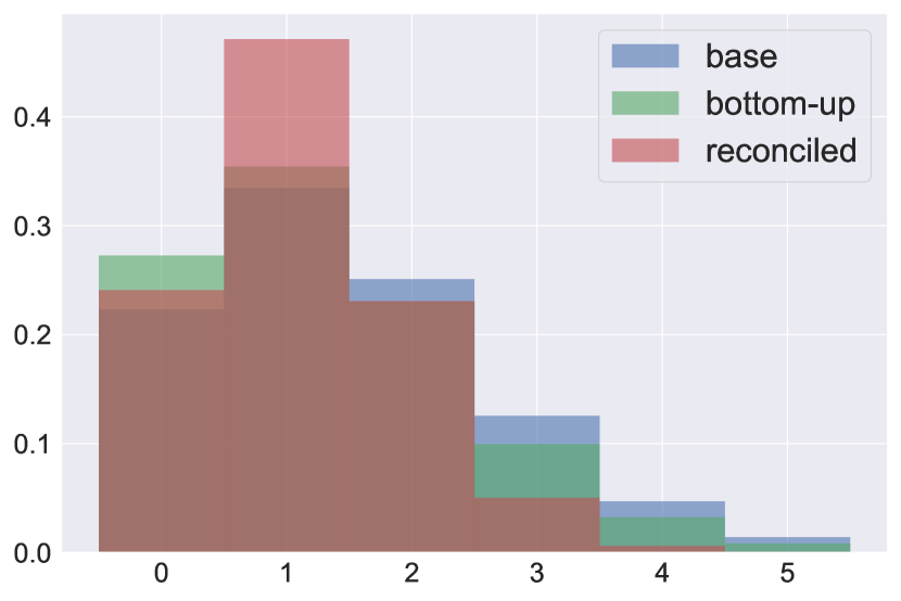
(a) Concordant-shift effect.

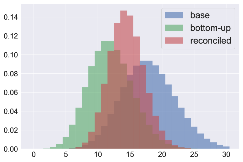
(b) Combination effect.

Figure 2: Base, bottom-up, and reconciled probability mass functions of $U$ in case of Poisson base forecasts. (a) $\widehat{\lambda}_{1}=0.5$, $\widehat{\lambda}_{2}=0.8$, $\widehat{\lambda}_{u}=1.5$ (b) $\widehat{\lambda}_{1}=5$, $\widehat{\lambda}_{2}=7$, $\widehat{\lambda}_{u}=18$

	concordant-shift effect			combination effect
	$p_{c}=0.25$			$p_{c}=0.04$
	base mean	rec. mean	$\Delta$	base mean	rec. mean	$\Delta$
$B_{1}$	0.50	0.43	-0.07	5.00	6.02	1.02
$B_{2}$	0.80	0.68	-0.12	7.00	8.43	1.43
$U$	1.50	1.11	-0.39	18.0	14.44	-3.56

Table 2: Mean before and after reconciliation; the base forecasts are Poisson.

3 Case study: modeling extreme market events

Credit default swaps (CDS) are financial instruments that guarantee insurance against the possible default of a given company (called “reference company”) to the buyer. The CDS price is a function of the probability of default estimated by the market for that company. Thus, a high value of the CDS spread corresponds to an increase in the risk of a company default.

Following Raunig and Scheicher (2011), an extreme market event takes place when the value of the CDS spread on a given day exceeds the 90-th percentile of its distribution in the last trading year. In particular, we forecast the extreme market events for the companies of the Euro Stoxx 50 index (https://www.stoxx.com/) in the period 2005-2018, which includes 3508 trading days. As in Agosto et al. (2020), we consider the 29 companies included in the index having a regularly quoted CDS and we divide them into five economic sectors: Financial (FIN), Information and Communication Technology (ICT), Manufacturing (MFG), Energy (ENG), and Trade (TRD). Following Agosto (2022), we start from the CDS spread time series retrieved from Bloomberg and we count the daily number of extreme events for each sector, obtaining five daily time series. The series include 3508 data points each; they have low counts and a high frequency of zeros (Table 3); they are all intermittent, with large average inter-demand interval (ADI).

Sector	Time series	Mean	Proportion of zeros	ADI
FIN	10	0.96	0.73	3.8
ICT	4	0.38	0.79	4.7
MFG	7	0.67	0.73	3.7
ENG	5	0.48	0.80	4.9
TRD	3	0.29	0.81	5.2

Table 3: Main characteristics of the count time series. A time series is considered intermittent if its ADI is >1.32 (Syntetos and Boylan, 2005).

Base forecasts and hierarchical structure

Figure 3: Hierarchical structure of the extreme events time series.

We organize the time series into a hierarchy with 5 bottom and 1 upper time series: the five economic sectors constitute the bottom level, while their sum constitutes the top level (Fig. 3).

We compute the base forecasts for the bottom time series (counts in the different sectors) using the model of Agosto (2022), whose predictive distribution is a multivariate negative binomial with a static vector of dispersion parameters and a time-varying vector of location parameters following a score-driven dynamics (Harvey, 2013). The model of Agosto (2022) extends to the multivariate case the modeling approach of Agosto et al. (2016), who proposed a Poisson autoregressive model with exogenous covariates (PARX) to measure systemic risk in the corporate default dynamics. According to Agosto (2022), the predictive distribution computed at time $t$ for the count of time $t+1$ in sector $i$ is:

$$\widehat{y}_{i,t+1}\sim NB(\mu_{i,t+1},\alpha_{i}),$$ (13)

where $\bm{\mu}_{t}$ is the $k\times 1$ vector of location parameters, $k$ is the number of sectors, and $\alpha_{i}\geq 0$. The model assumes the following dynamics:

$$\log(\bm{\mu}_{t+1})=\mathbf{C}+\mathbf{D}\log{\bm{\mu}_{t}}+\mathbf{E}\dfrac{\mathbf{y}_{t}-\bm{\mu}_{t}}{\bm{\alpha}^{T}\bm{\mu}_{t}+1},$$ (14)

where $\mathbf{C}$ is a $k\times 1$ vector, while $\mathbf{D}$ and $\mathbf{E}$ are $k\times k$ matrices (see Agosto (2022) for detailed properties and estimation details). Thus, the predicted event count in a given sector is a function of the past expectations ($\bm{\mu}_{t}$) and forecast errors ($\mathbf{y}_{t}-\bm{\mu}_{t}$) in the same sector and in the other sectors. The base forecasts for the upper time series are computed by fitting a univariate version of the model (Blasques et al., 2023) on the aggregate count time series.

The base forecasts for the bottom series measure financial risks at the sector level, accounting for the dependencies between sectors, through a shock propagation mechanism, besides an autoregressive component. The base upper forecasts express instead a measure of aggregate systemic financial risk.

3.1 Experimental procedure

As in Agosto (2022), we estimate the model parameters through in-sample maximum likelihood. We then compute the 1-day ahead base forecasts for time $t+1$ by conditioning the model on the counts observed up to time $t$.

We reconcile the in-sample base forecasts using importance sampling (Sect. 2.2). We perform 3508 reconciliations, drawing each time $N=100,000$ samples from the reconciled distribution; each reconciliation is almost instantaneous (<0.1 sec).

As recommended by Panagiotelis et al. (2023), we compare base and reconciled distributions through the energy score (ES, Székely and Rizzo (2013)):

$$ES(P_{t},\mathbf{y}_{t})=\mathbb{E}_{P_{t}}\left[\|\mathbf{y}_{t}-\mathbf{s}_{t}\|^{\beta}\right]-\frac{1}{2}\mathbb{E}_{P_{t}}\left[\|\mathbf{s}_{t}-\mathbf{s}_{t}^{\prime}\|^{\beta}\right],$$

where $P_{t}$ is the forecast distribution on the whole hierarchy, $\mathbf{s}_{t},\mathbf{s}_{t}^{\prime}$ are a pair of independent random variables distributed as $P_{t}$, and $\mathbf{y}_{t}$ is the vector of the actual values of all the time series at time $t$. We compute the ES, with $\beta=2$, using the sampling approach of Wickramasuriya (2023). We compute the ES of the joint predictive distribution of the upper and bottom time series; we thus have a single ES for the entire hierarchy.

Moreover, we evaluate the prediction intervals using the interval score (IS, Gneiting and Raftery (2007)):

$$\text{IS}_{\alpha}(l_{t},u_{t};y_{t})=(u_{t}-l_{t})+\frac{2}{\alpha}(l_{t}-y_{t})\mathbb{1}(y_{t}<l_{t})+\frac{2}{\alpha}(y_{t}-u_{t})\mathbb{1}(y_{t}>u_{t}),$$

where $\alpha\in(0,1)$, $l_{t}$ and $u_{t}$ are the lower and upper bounds of the $(1-\alpha)\times 100\,\%$ prediction interval and $y_{t}$ is the actual value of the time series at time $t$. We use $\alpha=0.1$, i.e. we score prediction interval whose nominal coverage is 90%.

Finally, we evaluate the point forecasts measuring the squared error (SE) and the absolute error (AE):

SE $$=\left(y_{t}-\hat{y}_{t\mid t-1}\right)^{2},$$

AE $$=\left|y_{t}-\hat{y}_{t\mid t-1}\right|,$$

where $\hat{y}_{t\mid t-1}$ denotes the optimal point forecast. The optimal point forecast depends on the error measure: it is the median of the predictive distribution for AE, and the expected value for SE (Kolassa, 2016, 2020).

Skill score

The skill score measures the improvement of the reconciled forecasts over the base forecasts. For example, the skill score for AE is defined as:

$$\text{skill}(\textit{reconc},\textit{base})=\frac{\text{AE}(\textit{base})-\text{AE}(\textit{reconc})}{\left(\text{AE}(\textit{base})+\text{AE}(\textit{reconc})\right)/2}.$$ (15)

For all indicators, a positive skill score implies an improvement of the reconciled forecast compared to the base forecasts, and vice versa. The skill score defined in (15) is symmetric, allowing to fairly compare base and reconciled forecasts. For instance, a skill score of 1 implies that the loss function has been reduced by three times: $(3-1)/((3+1)/2)=2/2=1$. Analogously, a skill score of $-1$ implies a three-fold worsening of the loss function. Moreover, the skill score is bounded between $-2$ and $2$. Di Fonzo and Girolimetto (2022) compare competing approaches by computing the geometric mean of the indicators. However, this is not suitable for count time series, where the SE and the AE are often zero.

	ALL	FIN	ICT	MFG	ENG	TRD
ES	0.89
IS	0.87	1.15	0.20	1.07	0.22	0.18
SE	0.82	1.10	1.11	1.07	1.12	1.11
AE	-0.02	-0.02	-0.02	-0.02	-0.02	-0.02

Table 4: Average skill scores for the different time series. Positive values indicate an improvement of the reconciled forecasts over the base forecasts. The ES is computed with respect to the joint distribution on the entire hierarchy.

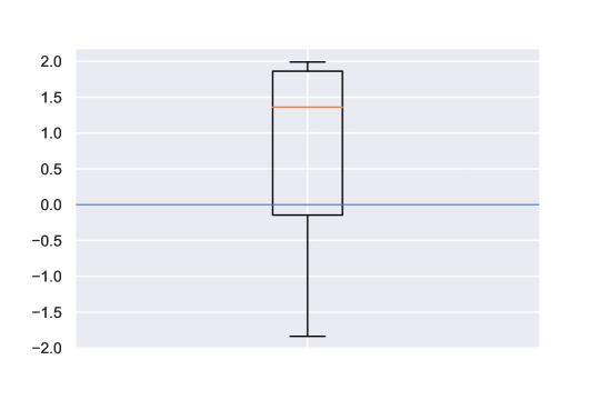
Figure 4: Boxplot of the skill scores on ES, over 3508 reconciliations.

	ALL	FIN	ICT	MFG	ENG	TRD
base	6.9	3.2	1.1	1.9	1.3	0.9
reconc.	3.3	2.1	0.9	1.2	1.0	0.8

Table 5: Width of the $90\%$ prediction interval, averaged over 3508 reconciliations.

	ALL	FIN	ICT	MFG	ENG	TRD
base	96%	98%	98%	98%	98%	99%
reconc.	91%	95%	97%	97%	97%	98%

Table 6: Coverage of the $90\%$ prediction intervals, assessed on 3508 reconciliations.

In Table 4 we report the skill scores averaged over the 3508 reconciliations. Reconciliation largely improves the ES (with an average skill score of $0.89$) and the IS (average skill score ranging between 0.2 and 1.1, depending on the chosen time series). The boxplot of the skill scores on ES on each day (Fig. 4) confirms the improvement due to reconciliation. As a further insight, reconciliation reduces by 15-50% the width of the prediction intervals (Table 6) without compromising their coverage (Table 6). We observe large skill scores (0.8-1) on the SE. On the other hand, the skill core on AE is close to 0. Indeed, often the median of the predictive distribution is already 0, and it does not change after reconciliation.

Hence, in our experiments, reconciliation yields a major improvement over the base forecasts, confirming the positive effect of probabilistic reconciliation (Corani et al., 2023; Zambon et al., 2024) and point forecast reconciliation (Kourentzes and Athanasopoulos, 2021) for intermittent time series.

Coherent vs optimal point forecast for the upper time series

Even if we have a reconciled distribution, only the SE-optimal point forecasts are coherent. The AE-optimal point forecasts, i.e., the medians of the reconciled distributions, are instead generally incoherent (Kolassa, 2022).

Hence, besides optimal point forecasts, we evaluate the coherent point forecasts: we take the sum of the medians of the reconciled bottom distributions and use it as upper point forecast. We compute the mean absolute error for the upper time series obtained using the AE-optimal, the coherent, and the base point forecasts (Table 7). As expected, the AE worsens by imposing coherence rather than optimality; yet, it remains better than the AE of the base forecasts.

	optimal	coherent	base
ALL	1.10	1.24	1.33

Table 7: Mean absolute error for the upper time series “ALL”.

3.2 Analysis of the reconciled mean and variance

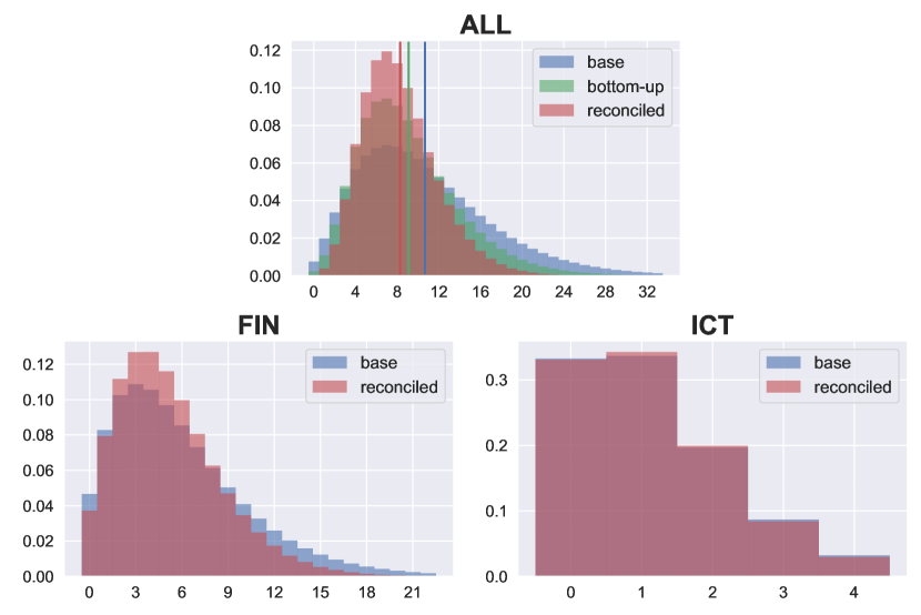
(a) Concordant-shift effect. The reduction of variance of the asymmetric distribution shortens the right tail and decreases the mean.

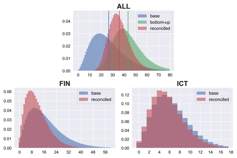
(b) Combination effect

Figure 5: Concordant-shift vs combination effect. We plot the base and reconciled probability mass functions for “ALL”, “FIN”, and “ICT”. For “ALL”, we also show the bottom-up pmf. The vertical lines correspond to the means of the distributions.

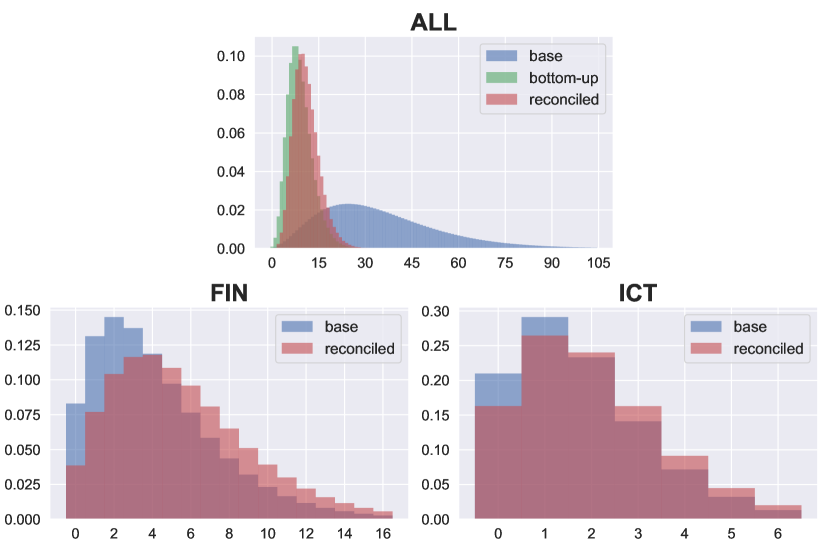
Figure 6: An example of reconciliation which increases the variance of the bottom forecasts, due to a large incoherence of the base forecasts (note the $X$-axis of “ALL”). Variance of “FIN”: $11.4$ (base), $14.3$ (reconciled). Variance of “ICT”: $2.2$ (base), $2.6$ (reconciled).

In most reconciliations (96%), we observe the concordant-shift effect, i.e., the reconciled upper mean is lower than both the bottom-up and the base upper mean. In Fig. 5(a), we show an example. Reconciliation largely reduces the variance of “ALL” and “FIN”, shortening the right tail of the distribution. Within the bottom time series, reconciliation mostly affects FIN, which is characterized by the largest counts and overdispersion. The predictive distribution for other time series, such as ICT (shown in figure), are less affected by reconciliation, being characterized by lower counts and variability. The reduction of the variance shifts the expected values towards zero, since the base distributions have a positive skewness.

In Fig. 5(b), we show an example of the combination effect. The reconciled distribution of “ALL” is a combination between its base forecast and the probabilistic bottom-up. Reconciliation decreases the expected values of the bottom time series, while increasing the expected value of the upper time series.

The variance of all the variables decreases in most cases (97%). However, in Fig. 6 we show an example in which the variance of the bottom variables increases after reconciliation because of large incoherence of the base forecasts. The forecast of the upper time series, which is characterized by large uncertainty, is instead sharply shifted towards smaller values.

4 Conclusions

We proved that reconciliation via conditioning decreases the variance of all variables in the Gaussian framework, while it can increase or decrease the variance of discrete variables, depending on the incoherence of the base forecasts. We also discussed two different effects that the reconciliation can have on the upper mean. The empirical analysis of time series of extreme market events confirmed our theoretical insights. We leave as future research the study of the theoretical properties of the reconciliation of other continuous non-Gaussian distributions, including skewed ones.

5 Acknowledgements

Work partially funded by the Swiss National Science Foundation (grant 200021_212164/1), by the Hasler foundation (project 23057), and by the European Union’s Horizon 2020 research and innovation programme (grant 101016233).

Appendix A Reconciled distribution in the Gaussian case

Bottom distribution

Let us define $\mathbf{T}\in\mathbb{R}^{n\times n}$ as

$$\mathbf{T}=\begin{bmatrix}\textbf{0}&\mathbf{I}_{m}\\ \mathbf{I}_{n-m}&-\mathbf{A}\end{bmatrix},$$

and let $\mathbf{Z}:=\mathbf{T}\widehat{\mathbf{Y}}$. Hence, $\mathbf{Z}$ is Gaussian:

$$\mathbf{Z}\sim\mathcal{N}\left(\mathbf{T}\widehat{\mathbf{y}},\,\mathbf{T}\widehat{\mathbf{\Sigma}}_{Y}\mathbf{T}^{T}\right).$$ (16)

We have

$$\mathbf{T}\widehat{\mathbf{y}} =\begin{bmatrix}\widehat{\mathbf{b}}\\ \widehat{\mathbf{u}}-\mathbf{A}\widehat{\mathbf{b}}\end{bmatrix},$$

$$\mathbf{T}\widehat{\mathbf{\Sigma}}_{Y}\mathbf{T}^{T} =\begin{bmatrix}\widehat{\mathbf{\Sigma}}_{B}&\widehat{\mathbf{\Sigma}}_{UB}^{T}-\widehat{\mathbf{\Sigma}}_{B}\mathbf{A}^{T}\\ \widehat{\mathbf{\Sigma}}_{UB}-\mathbf{A}\widehat{\mathbf{\Sigma}}_{B}&\mathbf{Q}\end{bmatrix},$$ (17)

where $\mathbf{Q}=\widehat{\mathbf{\Sigma}}_{U}-\widehat{\mathbf{\Sigma}}_{UB}\mathbf{A}^{T}-\mathbf{A}\widehat{\mathbf{\Sigma}}_{UB}^{T}+\mathbf{A}\widehat{\mathbf{\Sigma}}_{B}\mathbf{A}^{T}$. Since

$$\mathbf{Z}=\begin{bmatrix}\widehat{\mathbf{B}}\\ \widehat{\mathbf{U}}-\mathbf{A}\widehat{\mathbf{B}}\end{bmatrix}=:\begin{bmatrix}\mathbf{Z}_{1}\\ \mathbf{Z}_{2}\end{bmatrix},$$

the reconciled bottom distribution is given by the conditional distribution of $\mathbf{Z}_{1}$ given $\mathbf{Z}_{2}=0$. Since the covariance matrix $\widehat{\mathbf{\Sigma}}_{Y}$ is assumed to be positive definite, the covariance matrix $\mathbf{Q}$ of $\mathbf{Z}_{2}$ is also positive definite; hence, we have

$$\mathbf{Z}_{1}\,|\,\mathbf{Z}_{2}=0\sim\mathcal{N}\left(\widetilde{\mathbf{b}},\,\widetilde{\mathbf{\Sigma}}_{B}\right),$$

where

$$\widetilde{\mathbf{b}} =\widehat{\mathbf{b}}+\left(\widehat{\mathbf{\Sigma}}_{UB}^{T}-\widehat{\mathbf{\Sigma}}_{B}\mathbf{A}^{T}\right)\mathbf{Q}^{-1}(\mathbf{A}\widehat{\mathbf{b}}-\widehat{\mathbf{u}}),$$ (18)

$$\widetilde{\mathbf{\Sigma}}_{B} =\widehat{\mathbf{\Sigma}}_{B}-\left(\widehat{\mathbf{\Sigma}}_{UB}^{T}-\widehat{\mathbf{\Sigma}}_{B}\mathbf{A}^{T}\right)\mathbf{Q}^{-1}\left(\widehat{\mathbf{\Sigma}}_{UB}^{T}-\widehat{\mathbf{\Sigma}}_{B}\mathbf{A}^{T}\right)^{T}.$$ (19)

Upper distribution

Since $\widetilde{\mathbf{U}}=\mathbf{A}\widetilde{\mathbf{B}}$, we have that $\widetilde{\mathbf{U}}\sim\mathcal{N}\left(\widetilde{\mathbf{u}},\,\widetilde{\mathbf{\Sigma}}_{U}\right)$, with

$$\widetilde{\mathbf{u}}=\mathbf{A}\widetilde{\mathbf{b}},\qquad\widetilde{\mathbf{\Sigma}}_{U}=\mathbf{A}\widetilde{\mathbf{\Sigma}}_{B}\mathbf{A}^{T}.$$ (20)

If we define $\mathbf{D}:=\widehat{\mathbf{\Sigma}}_{U}-\widehat{\mathbf{\Sigma}}_{UB}\mathbf{A}^{T}$, from (20) and (18) we have

$$\widetilde{\mathbf{u}} =\mathbf{A}\widehat{\mathbf{b}}+\left(\mathbf{A}\widehat{\mathbf{\Sigma}}_{UB}^{T}-\mathbf{A}\widehat{\mathbf{\Sigma}}_{B}\mathbf{A}^{T}\right)\mathbf{Q}^{-1}(\mathbf{A}\widehat{\mathbf{b}}-\widehat{\mathbf{u}})$$

$$=\mathbf{A}\widehat{\mathbf{b}}+\left(\mathbf{D}-\mathbf{Q}\right)\mathbf{Q}^{-1}(\mathbf{A}\widehat{\mathbf{b}}-\widehat{\mathbf{u}})$$

$$=\mathbf{A}\widehat{\mathbf{b}}+\mathbf{D}\mathbf{Q}^{-1}(\mathbf{A}\widehat{\mathbf{b}}-\widehat{\mathbf{u}})-(\mathbf{A}\widehat{\mathbf{b}}-\widehat{\mathbf{u}})$$

$$=\widehat{\mathbf{u}}+\left(\widehat{\mathbf{\Sigma}}_{U}-\widehat{\mathbf{\Sigma}}_{UB}\mathbf{A}^{T}\right)\mathbf{Q}^{-1}(\mathbf{A}\widehat{\mathbf{b}}-\widehat{\mathbf{u}}).$$

Moreover, from (20) and (19):

$$\widetilde{\mathbf{\Sigma}}_{U} =\mathbf{A}\widehat{\mathbf{\Sigma}}_{B}\mathbf{A}^{T}-\left(\mathbf{A}\widehat{\mathbf{\Sigma}}_{UB}^{T}-\mathbf{A}\widehat{\mathbf{\Sigma}}_{B}\mathbf{A}^{T}\right)\mathbf{Q}^{-1}\left(\mathbf{A}\widehat{\mathbf{\Sigma}}_{UB}^{T}-\mathbf{A}\widehat{\mathbf{\Sigma}}_{B}\mathbf{A}^{T}\right)^{T}$$

$$=\mathbf{A}\widehat{\mathbf{\Sigma}}_{B}\mathbf{A}^{T}-\left(\mathbf{D}-\mathbf{Q}\right)\mathbf{Q}^{-1}\left(\mathbf{D}^{T}-\mathbf{Q}\right)$$

$$=\mathbf{A}\widehat{\mathbf{\Sigma}}_{B}\mathbf{A}^{T}-\mathbf{D}\mathbf{Q}^{-1}\mathbf{D}^{T}+\mathbf{D}+\mathbf{D}^{T}-\mathbf{Q}$$

$$=\widehat{\mathbf{\Sigma}}_{U}-\left(\widehat{\mathbf{\Sigma}}_{U}-\widehat{\mathbf{\Sigma}}_{UB}\mathbf{A}^{T}\right)\mathbf{Q}^{-1}\left(\widehat{\mathbf{\Sigma}}_{U}-\widehat{\mathbf{\Sigma}}_{UB}\mathbf{A}^{T}\right)^{T}.$$

Relation to Corani et al. (2020)

In Corani et al. (2020), the reconciliation framework was defined is the following way:

• $\mathbf{B}^{\prime}\sim\mathcal{N}\big{(}\widehat{\mathbf{b}},\widehat{\mathbf{\Sigma}}_{B}\big{)}$,

• $\widehat{\mathbf{U}}^{\prime}=\mathbf{A}\mathbf{B}^{\prime}+\mathbf{\epsilon}^{u}$,

where the error term $\mathbf{\epsilon}^{u}$ was assumed to have zero mean and to be jointly Gaussian with $\mathbf{B}^{\prime}$. The reconciled distribution on the bottom time series was then obtained via a Bayes’ update by conditioning on $\widehat{\mathbf{U}}^{\prime}=\widehat{\mathbf{u}}$, the point forecast for the upper time series.

In this paper, we adopt a slightly different framework. We assume that the base forecasts are jointly Gaussian:

$$\widehat{\mathbf{Y}}=\begin{bmatrix}\widehat{\mathbf{U}}\\ \widehat{\mathbf{B}}\end{bmatrix}\sim\mathcal{N}\left(\widehat{\mathbf{y}},\,\widehat{\mathbf{\Sigma}}_{Y}\right),$$

hence we have $\widehat{\mathbf{B}}\sim\mathcal{N}\big{(}\widehat{\mathbf{b}},\widehat{\mathbf{\Sigma}}_{B}\big{)}$ and $\widehat{\mathbf{U}}\sim\mathcal{N}\big{(}\widehat{\mathbf{u}},\widehat{\mathbf{\Sigma}}_{U}\big{)}$. The reconciled distribution on the bottom time series is obtained by conditioning on $\widehat{\mathbf{U}}=\mathbf{A}\widehat{\mathbf{B}}$. This is equivalent to the framework of Corani et al. (2020), if we set $\widehat{\mathbf{B}}=\mathbf{B}^{\prime}$ and $\widehat{\mathbf{U}}=\widehat{\mathbf{u}}-\mathbf{\epsilon}^{u}$. The hypothesis of joint normality of $(\mathbf{B}^{\prime},\,\mathbf{\epsilon}^{u})$ is thus replaced by the hypothesis of joint normality of $(\widehat{\mathbf{B}},\,\widehat{\mathbf{U}})$. Indeed, (18) and (19) are precisely the formulae (11) and (12) in Corani et al. (2020), if we set

$$\widehat{\mathbf{\Sigma}}_{UB}=-k_{h}\mathbf{M}_{1}^{T},\quad\widehat{\mathbf{\Sigma}}_{B}=k_{h}\widehat{\mathbf{\Sigma}}_{B,1},\quad\widehat{\mathbf{\Sigma}}_{U}=k_{h}\widehat{\mathbf{\Sigma}}_{U,1}.$$ (21)

Note that in this paper we only deal with one step ahead forecasts (i.e., $h=1$), hence $k_{h}=1$ and can be omitted. Since the covariance matrices correspond to those of Corani et al. (2020), as shown in (21), we conclude that $\widehat{\mathbf{\Sigma}}_{Y}$ can be estimated as the covariance matrix of the residuals of the entire hierarchy.

Appendix B Proof of Proposition 1

First, $\mathbf{Q}$ is positive definite, as it is the covariance matrix of $\widehat{\mathbf{U}}-\mathbf{A}\widehat{\mathbf{B}}$ (see A). Hence, $\mathbf{Q}^{-1}$ is also positive definite, and the matrices

$$\mathbf{G}:=\left(\widehat{\mathbf{\Sigma}}_{UB}^{T}-\widehat{\mathbf{\Sigma}}_{B}\mathbf{A}^{T}\right)\mathbf{Q}^{-1}\left(\widehat{\mathbf{\Sigma}}_{UB}^{T}-\widehat{\mathbf{\Sigma}}_{B}\mathbf{A}^{T}\right)^{T},$$

$$\mathbf{H}:=\left(\widehat{\mathbf{\Sigma}}_{U}-\widehat{\mathbf{\Sigma}}_{UB}\mathbf{A}^{T}\right)\mathbf{Q}^{-1}\left(\widehat{\mathbf{\Sigma}}_{U}-\widehat{\mathbf{\Sigma}}_{UB}\mathbf{A}^{T}\right)^{T},$$

are positive semi-definite.

From (7), we have that, for each $i=1,\dots,m$

$$\textrm{Var}(\widetilde{B}_{i})=\textrm{Var}(\widehat{B}_{i})-G_{ii}\leq\textrm{Var}(\widehat{B}_{i}),$$

as $G_{ii}\geq 0$ since the matrix $\mathbf{G}$ is positive semi-definite. Analogously, we have

$$\textrm{Var}(\widetilde{U}_{j})=\textrm{Var}(\widehat{U}_{j})-H_{jj}\leq\textrm{Var}(\widehat{U}_{j}),$$

for all $j=1,\dots,n-m$.

Appendix C Proof of Proposition 2

Let us denote $Z:=\mathbb{1}_{\{\widehat{\mathbf{U}}=\mathbf{A}\widehat{\mathbf{B}}\}}$, so that $Z=1$ when the constraint is satisfied, and $0$ otherwise. By the law of total variance (Weiss, 2005), for any $j=1,\dots,m$, we have

$$\textrm{Var}\left(\widehat{B}_{j}\right)=\mathbb{E}_{Z}\left[\textrm{Var}\big{(}\widehat{B}_{j}|Z\big{)}\right]+\textrm{Var}_{Z}\left(\mathbb{E}\big{[}\widehat{B}_{j}|Z\big{]}\right).$$ (22)

Since

$$\mathbb{E}\big{[}\widehat{B}_{j}|Z\big{]}=\begin{cases}\mathbb{E}\big{[}\widehat{B}_{j}|\widehat{\mathbf{U}}=\mathbf{A}\widehat{\mathbf{B}}\big{]}\quad\text{if }Z=1\\ \mathbb{E}\big{[}\widehat{B}_{j}|\widehat{\mathbf{U}}\neq\mathbf{A}\widehat{\mathbf{B}}\big{]}\quad\text{if }Z=0,\end{cases}$$

we have that $\mathbb{E}[\widehat{B}_{j}|Z]=a+(b-a)\,Z$, where $a:=\mathbb{E}[\widehat{B}_{j}|\widehat{\mathbf{U}}\neq\mathbf{A}\widehat{\mathbf{B}}]$ and $b:=\mathbb{E}[\widehat{B}_{j}|\widehat{\mathbf{U}}=\mathbf{A}\widehat{\mathbf{B}}]$. Note that $Z\sim\text{Bernoulli}(p_{c})$, with $p_{c}:=Prob(\widehat{\mathbf{U}}=\mathbf{A}\widehat{\mathbf{B}})$. Hence

$$\textrm{Var}_{Z}\left(\mathbb{E}\big{[}\widehat{B}_{j}|Z\big{]}\right) =\textrm{Var}_{Z}\big{(}a+(b-a)\,Z\big{)}$$

$$=(b-a)^{2}p_{c}(1-p_{c}).$$ (23)

Moreover, since

$$\textrm{Var}\big{[}\widehat{B}_{j}|Z\big{]}=\begin{cases}\textrm{Var}\big{[}\widehat{B}_{j}|\widehat{\mathbf{U}}=\mathbf{A}\widehat{\mathbf{B}}\big{]}\quad\text{if }Z=1\\ \textrm{Var}\big{[}\widehat{B}_{j}|\widehat{\mathbf{U}}\neq\mathbf{A}\widehat{\mathbf{B}}\big{]}\quad\text{if }Z=0,\end{cases}$$

we have

$$\mathbb{E}_{Z}\left[\textrm{Var}\big{(}\widehat{B}_{j}|Z\big{)}\right]=p_{c}\,\textrm{Var}\big{[}\widehat{B}_{j}|\widehat{\mathbf{U}}=\mathbf{A}\widehat{\mathbf{B}}\big{]}+(1-p_{c})\,\textrm{Var}\big{[}\widehat{B}_{j}|\widehat{\mathbf{U}}\neq\mathbf{A}\widehat{\mathbf{B}}\big{]}.$$ (24)

From (22), (23), and (24), we obtain

$$\textrm{Var}\big{(}\widehat{B}_{j}\big{)} =p_{c}\,\textrm{Var}\big{[}\widehat{B}_{j}|\widehat{\mathbf{U}}=\mathbf{A}\widehat{\mathbf{B}}\big{]}+(1-p_{c})\,\textrm{Var}\big{[}\widehat{B}_{j}|\widehat{\mathbf{U}}\neq\mathbf{A}\widehat{\mathbf{B}}\big{]}$$

$$\,+p_{c}(1-p_{c})\,(a-b)^{2},$$

from which

$$\textrm{Var}\big{[}\widetilde{B}_{j}\big{]} =\textrm{Var}\big{[}\widehat{B}_{j}|\widehat{\mathbf{U}}=\mathbf{A}\widehat{\mathbf{B}}\big{]}$$

$$=\frac{\textrm{Var}\big{(}\widehat{B}_{j}\big{)}-(1-p_{c})\,\textrm{Var}\big{[}\widehat{B}_{j}|\widehat{\mathbf{U}}\neq\mathbf{A}\widehat{\mathbf{B}}\big{]}-p_{c}(1-p_{c})\,(a-b)^{2}}{p_{c}}.$$

Appendix D Bernoulli example

Let us denote by $\widehat{\pi}_{1}$ and $\widehat{\pi}_{2}$ the probability mass functions of $\widehat{B}_{1}$ and $\widehat{B}_{2}$, so that $\widehat{\pi}_{1}(0)=1-\widehat{p}_{1}$, $\widehat{\pi}_{1}(1)=\widehat{p}_{1}$, and $\widehat{\pi}_{1}(k)=0$ for any $k\neq 0,1$. The probability mass function $\widehat{\pi}_{U}$ of $\widehat{U}$ is defined as $\widehat{\pi}_{U}(0)=\widehat{q}_{0}$, $\widehat{\pi}_{U}(1)=\widehat{q}_{1}$, $\widehat{\pi}_{U}(2)=\widehat{q}_{2}$, and $\widehat{\pi}_{U}(k)=0$ for any $k\neq 0,1,2$.

Since, from (3), the reconciled probability mass function $\widetilde{\pi}_{B}$ is given by

$$\widetilde{\pi}_{B}(b_{1},b_{2})\propto\widehat{\pi}_{1}(b_{1})\widehat{\pi}_{2}(b_{2})\widehat{\pi}_{U}(b_{1}+b_{2}),$$

the reconciled bottom distribution can be expressed as

$$(\widetilde{B}_{1},\widetilde{B}_{2})=\begin{cases}(0,0)\qquad\text{prob}=(1-\widehat{p}_{1})(1-\widehat{p}_{2})\widehat{q}_{0}\,/\,p_{c}\\ (1,0)\qquad\text{prob}=\widehat{p}_{1}(1-\widehat{p}_{2})\widehat{q}_{1}\,/\,p_{c}\\ (0,1)\qquad\text{prob}=(1-\widehat{p}_{1})\widehat{p}_{2}\widehat{q}_{1}\,/\,p_{c}\\ (1,1)\qquad\text{prob}=\widehat{p}_{1}\widehat{p}_{2}\widehat{q}_{2}\,/\,p_{c},\end{cases}$$

where the normalizing constant $p_{c}:=(1-\widehat{p}_{1})(1-\widehat{p}_{2})\widehat{q}_{0}+\widehat{p}_{1}(1-\widehat{p}_{2})\widehat{q}_{1}+(1-\widehat{p}_{1})\widehat{p}_{2}\widehat{q}_{1}+\widehat{p}_{1}\widehat{p}_{2}\widehat{q}_{2}$ is the probability of coherence, defined in (12). Hence

$$\widetilde{B}_{1}\sim\textit{Bernoulli}\,(\widetilde{p}_{1}),\quad\widetilde{B}_{2}\sim\textit{Bernoulli}\,(\widetilde{p}_{2}),$$

with

$$\widetilde{p}_{1} =\frac{[(1-\widehat{p}_{2})\widehat{q}_{1}+\widehat{p}_{2}\widehat{q}_{2}]\widehat{p}_{1}}{S},$$

$$\widetilde{p}_{2} =\frac{[(1-\widehat{p}_{1})\widehat{q}_{1}+\widehat{p}_{1}\widehat{q}_{2}]\widehat{p}_{2}}{S}.$$ (25)

Finally,

$$\widetilde{U}=\begin{cases}0\qquad\text{prob}=(1-\widehat{p}_{1})(1-\widehat{p}_{2})\widehat{q}_{0}/S\\ 1\qquad\text{prob}=(\widehat{p}_{1}+\widehat{p}_{2}-2\widehat{p}_{1}\widehat{p}_{2})\widehat{q}_{1}/S\\ 2\qquad\text{prob}=\widehat{p}_{1}\widehat{p}_{2}\widehat{q}_{2}/S.\end{cases}$$ (26)

References

• Agosto (2022) Agosto, A., 2022. Multivariate score-driven models for count time series to assess financial contagion doi:https://dx.doi.org/10.2139/ssrn.4119895.
• Agosto et al. (2020) Agosto, A., Ahelegbey, D.F., Giudici, P., 2020. Tree networks to assess financial contagion. Economic Modelling 85, 349–366.
• Agosto et al. (2016) Agosto, A., Cavaliere, G., Kristensen, D., Rahbek, A., 2016. Modeling corporate defaults: Poisson autoregressions with exogenous covariates (parx). Journal of Empirical Finance 38, 640–663.
• Athanasopoulos et al. (2017) Athanasopoulos, G., Hyndman, R.J., Kourentzes, N., Petropoulos, F., 2017. Forecasting with temporal hierarchies. European Journal of Operational Research 262, 60–74.
• Azzimonti et al. (2023) Azzimonti, D., Rubattu, N., Zambon, L., Corani, G., 2023. bayesRecon: Probabilistic Reconciliation via Conditioning. R package version 0.1.2.
• Blasques et al. (2023) Blasques, F., Holỳ, V., Tomanová, P., 2023. Zero-inflated autoregressive conditional duration model for discrete trade durations with excessive zeros. Studies in Nonlinear Dynamics & Econometrics doi:doi:10.1515/snde-2022-0008.
• Corani et al. (2020) Corani, G., Azzimonti, D., Augusto, J.P., Zaffalon, M., 2020. Probabilistic reconciliation of hierarchical forecast via Bayes’ rule., in: Proc. European Conf. On Machine Learning and Knowledge Discovery in Database ECML/PKDD, pp. 211–226.
• Corani et al. (2023) Corani, G., Azzimonti, D., Rubattu, N., 2023. Probabilistic reconciliation of count time series. International Journal of Forecasting doi:https://doi.org/10.1016/j.ijforecast.2023.04.003.
• Di Fonzo and Girolimetto (2022) Di Fonzo, T., Girolimetto, D., 2022. Forecast combination-based forecast reconciliation: Insights and extensions. International Journal of Forecasting doi:https://doi.org/10.1016/j.ijforecast.2022.07.001.
• Elvira and Martino (2021) Elvira, V., Martino, L., 2021. Advances in importance sampling. Wiley StatsRef-Statistics Reference Online .
• Gelman (2011) Gelman, A., 2011. Adding more information can make the variance go up (depending on your model). https://statmodeling.stat.columbia.edu/2011/07/20/adding_more_inf/.
• Gelman et al. (2013) Gelman, A., Carlin, J., Stern, H., Dunson, D., Vehtari, A., Rubin, D., 2013. Bayesian Data Analysis (3rd ed.). Chapman and Hall/CRC.
• Gneiting and Raftery (2007) Gneiting, T., Raftery, A.E., 2007. Strictly proper scoring rules, prediction, and estimation. Journal of the American Statistical Association 102, 359–378.
• Harvey (2013) Harvey, A.C., 2013. Dynamic Models for Volatility and Heavy Tails: With Applications to Financial and Economic Time Series. Cambridge University Press, New York.
• Hollyman et al. (2021) Hollyman, R., Petropoulos, F., Tipping, M.E., 2021. Understanding forecast reconciliation. European Journal of Operational Research 294, 149–160.
• Hollyman et al. (2022) Hollyman, R., Petropoulos, F., Tipping, M.E., 2022. Hierarchies everywhere–managing & measuring uncertainty in hierarchical time series. arXiv:2209.15583 .
• Hyndman et al. (2011) Hyndman, R.J., Ahmed, R.A., Athanasopoulos, G., Shang, H.L., 2011. Optimal combination forecasts for hierarchical time series. Computational Statistics & Data Analysis 55, 2579 – 2589.
• Jeon et al. (2019) Jeon, J., Panagiotelis, A., Petropoulos, F., 2019. Probabilistic forecast reconciliation with applications to wind power and electric load. European Journal of Operational Research 279, 364–379.
• Kolassa (2016) Kolassa, S., 2016. Evaluating predictive count data distributions in retail sales forecasting. International Journal of Forecasting 32, 788–803.
• Kolassa (2020) Kolassa, S., 2020. Why the “best” point forecast depends on the error or accuracy measure. International Journal of Forecasting 36, 208–211.
• Kolassa (2022) Kolassa, S., 2022. Do we want coherent hierarchical forecasts, or minimal mapes or maes? (we won’t get both!). International Journal of Forecasting doi:https://doi.org/10.1016/j.ijforecast.2022.11.006.
• Kourentzes and Athanasopoulos (2021) Kourentzes, N., Athanasopoulos, G., 2021. Elucidate structure in intermittent demand series. European Journal of Operational Research 288, 141–152.
• Panagiotelis et al. (2021) Panagiotelis, A., Athanasopoulos, G., Gamakumara, P., Hyndman, R.J., 2021. Forecast reconciliation: A geometric view with new insights on bias correction. International Journal of Forecasting 37, 343–359.
• Panagiotelis et al. (2023) Panagiotelis, A., Gamakumara, P., Athanasopoulos, G., Hyndman, R.J., 2023. Probabilistic forecast reconciliation: Properties, evaluation and score optimisation. European Journal of Operational Research 306, 693–706.
• Rangapuram et al. (2021) Rangapuram, S.S., Werner, L.D., Benidis, K., Mercado, P., Gasthaus, J., Januschowski, T., 2021. End-to-end learning of coherent probabilistic forecasts for hierarchical time series, in: Proc. 38th Int. Conference on Machine Learning (ICML), pp. 8832–8843.
• Raunig and Scheicher (2011) Raunig, B., Scheicher, M., 2011. A value-at-risk analysis of credit default swaps. The Journal of Risk 13, 3.
• Syntetos and Boylan (2005) Syntetos, A.A., Boylan, J.E., 2005. The accuracy of intermittent demand estimates. International Journal of Forecasting 21, 303–314.
• Székely and Rizzo (2013) Székely, G.J., Rizzo, M.L., 2013. Energy statistics: A class of statistics based on distances. Journal of statistical planning and inference 143, 1249–1272.
• Taieb et al. (2021) Taieb, S.B., Taylor, J.W., Hyndman, R.J., 2021. Hierarchical probabilistic forecasting of electricity demand with smart meter data. Journal of the American Statistical Association 116, 27–43.
• Weiss (2005) Weiss, N.A., 2005. A Course in Probability. Pearson.
• Wickramasuriya (2021) Wickramasuriya, S.L., 2021. Properties of point forecast reconciliation approaches. arXiv:2103.11129.
• Wickramasuriya (2023) Wickramasuriya, S.L., 2023. Probabilistic forecast reconciliation under the gaussian framework. Journal of Business & Economic Statistics doi:10.1080/07350015.2023.2181176.
• Wickramasuriya et al. (2019) Wickramasuriya, S.L., Athanasopoulos, G., Hyndman, R.J., 2019. Optimal forecast reconciliation for hierarchical and grouped time series through trace minimization. Journal of the American Statistical Association 114, 804–819.
• Zambon et al. (2024) Zambon, L., Azzimonti, D., Corani, G., 2024. Efficient probabilistic reconciliation of forecasts for real-valued and count time series. Statistics and Computing 34, 21.