Blind Inpainting with Object-aware Discrimination for Artificial Marker Removal

Abstract

Medical images often contain artificial markers added by doctors, which can negatively affect the accuracy of AI-based diagnosis. To address this issue and recover the missing visual contents, inpainting techniques are highly needed. However, existing inpainting methods require manual mask input, limiting their application scenarios. In this paper, we introduce a novel blind inpainting method that automatically completes visual contents without specifying masks for target areas in an image. Our proposed model includes a mask-free reconstruction network and an object-aware discriminator. The reconstruction network consists of two branches that predict the corrupted regions with artificial markers and simultaneously recover the missing visual contents. The object-aware discriminator relies on the powerful recognition capabilities of the dense object detector to ensure that the markers of reconstructed images cannot be detected in any local regions. As a result, the reconstructed image can be close to the clean one as much as possible. Our proposed method is evaluated on different medical image datasets, covering multiple imaging modalities such as ultrasound (US), magnetic resonance imaging (MRI), and electron microscopy (EM), demonstrating that our method is effective and robust against various unknown missing region patterns.

1 Introduction

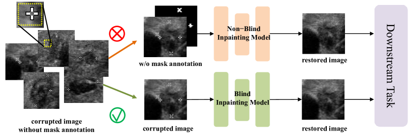
Figure 1: Blind inpainting model vs. Non-blind inpainting model. The blind inpainting model is capable of effectively restoring corrupted images without the need for mask annotation.

Recent advancements in artificial intelligence (AI) techniques have led to an increased interest in AI-based diagnostics among researchers [20]. Among them, medical imaging plays a pivotal role in the healthcare sector for diagnosis and treatment [6]. However, medical images often contain artificial markers added by doctors to highlight lesion regions, as shown in Fig. 1. While these markers are useful for human diagnosis, they can negatively impact deep learning-based lesion detectors and classifiers. Therefore, there is a critical need to reconstruct clean images by removing such markers and restoring missing visual content, especially if there is a large amount of historical unclean data. Inpainting methods are commonly used for image completion [9], and over the past decade, numerous studies in the literature have focused on developing efficient and robust inpainting methods, including GAN-based [29, 13], gated convolution-based [27], fourier-based [23], transformer-based [11, 8, 15] methods, diffusion-based [25, 17, 14, 5], etc. Inpainting is also widely employed in medical imaging. Dong et al. [7] propose a simultaneous X-Ray CT image reconstruction and Radon domain inpainting model using wavelet frame based regularization. Belli et al. [3] demonstrate how the context encoder architecture under adversarial training can effectively be used for inpainting in chest X-ray images. IpA-MedGAN [2] is illustrated to perform well for the inpainting of brain MR images. Rouzrokh et al. [19] present a leveraging diffusion models for multitask brain tumor inpainting.

However, recovering corrupted regions of artificial markers in images often requires manually drawing a mask as input to the inpainting model. This can be inconvenient, time-consuming, and error-prone, which limits its practicality. Blind inpainting methods [16] offer a more suitable solution as they do not require additional masks. For example, combining sparse coding and deep neural networks pre-trained with denoising auto-encoders, Xie et al. [26] use a non-linear approach to tackle the problem of blind inpainting of complex patterns. Afonso et al. [1] present an iterative method based on alternating minimization. Based on a fully convolutional neural network, BICNN [4] directly learns an end-to-end mapping between corrupted and ground truth pairs. VC-Net [24] performs well against unseen degradation patterns with sequentially connected mask prediction and inpainting networks. However, existing works still have difficulty in localizing the corrupted regions, leading to sub-optimal solutions in the image completion.

In this work, we focus on solving this challenging blind inpainting task by designing an efficient network that relaxes the restriction of mask as well as maintaining a good performance. We propose a novel end-to-end blind inpainting framework with mask-free reconstruction and object-aware discrimination. With two branches predicting corrupted regions and recovering missing visual content, and an object-aware discriminator for adversarial training, our approach produces reconstructions closely resembling clean images.

In summary, this paper makes the following contributions: 1) We propose a novel blind inpainting network for artificial marker removal in medical images. 2) We propose a two-branch reconstruction network for blind inpainting, which can simultaneously detect artificial markers and recover the missing visual contents. 3) We employ the object-aware discrimination by a dense object detector to ensure the reconstructed images are close to clean ones. 4) Our method outperforms other existing blind inpainting methods with a large margin on several medical image datasets with variant modalities, such as ultrasound (US), magnetic resonance imaging (MRI), and electron microscopy (EM), demonstrating the effectiveness of our method.

2 Method

2.1 Overview

The blind image inpainting task can be described as follows. Given an input corrupted image $I$ with artificial markers, we aim to learn a reconstruction network $f_{\theta}$ to obtain a clean image $\hat{I}$ with artificial markers removed, where $\theta$ are the network parameters to be learned. This blind inpainting task is different from the general inpainting task since the masks of corrupted regions are not provided in the inference stage.

In this paper, we introduce a novel blind inpainting framework for artificial marker removal in medical images, as shown in Fig. 2. It contains a mask-free reconstruction network and an object-aware discriminator. The reconstruction network has the ability to automatically localize the corrupted regions and inpaint the missing information simultaneously, thereby relaxing the constraint of using specific masks for target areas. In addition, the object-aware discriminator incorporates an object detector to enhance discrimination performance, demonstrating the feasibility of integrating object detectors into discriminative models. Details are described in following subsections.

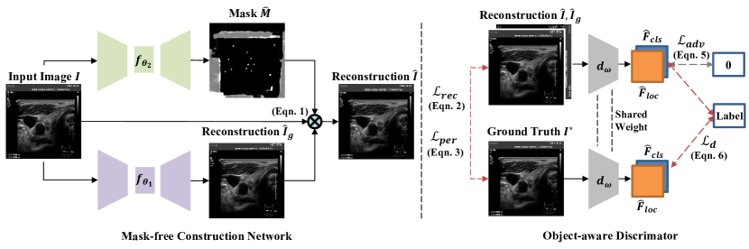
Figure 2: The proposed blind inpainting model, which consists of a two-branch reconstruction network $f_{\theta}$ and an object-aware discriminator $d_{\omega}$. In the two-branch reconstruction network, one branch $f_{\theta_{1}}$ implements the inpainting task, while the other branch $f_{\theta_{2}}$ estimates mask of corrupted regions. The object-aware discriminator follows the structure of dense object detectors to ensure the localization of artificial markers.

2.2 Mask-free Reconstruction Network

The mask-free reconstruction network follows the setting of blind inpainting framework that no masks are provided. To guide the reconstruction network to focus on the inpainting in the corrupted regions (which are unknown to the network), we use a two-branch architecture in the reconstruction network, which localizes corrupted regions and fills in the missing information, respectively. The reconstruction network $f_{\theta}$ is divided into two branches, $f_{\theta_{1}}$ and $f_{\theta_{2}}$, with the same structure and different parameters. Each branch has an upsampler-convolution-downsampler structure, based on gated convolution [27]. Specifically, $f_{\theta_{1}}$ implements the inpainting task, while $f_{\theta_{2}}$ estimates mask of corrupted regions. The reconstruction can be formulated as follows,

$$\hat{I}_{g}=f_{\theta_{1}}(I),$$ (1)

$$\hat{M}=f_{\theta_{2}}(I),$$

$$\hat{I}=\hat{M}\odot\hat{I}_{g}+(1-\hat{M})\odot I,$$

where $\odot$ represents the elementwise product. The mask of corrupted regions is implicitly learned and the reconstruction is supervised by the clean image $I^{*}$ with the $l_{1}$ loss as follows,

$$\mathcal{L}_{\text{rec}}(\theta)=\|I^{*}-\hat{I}_{g}\|_{1}+\|I^{*}-\hat{I}\|_{1},$$ (2)

where $\theta=\{\theta_{1},\theta_{2}\}$.

In addition, we also constrain the feature maps of the reconstructed image with perceptual loss as follows,

$$\mathcal{L}_{\text{per}}(\theta)=\|\phi(I^{*})-\phi(\hat{I}_{g})\|_{2}+\|\phi(I^{*})-\phi(\hat{I})\|_{2},$$ (3)

where $\phi(\cdot)$ denotes the layer activation of a pre-trained VGG-16 [21] network.

2.3 Object-aware Discrimination

Since the artificial markers in the corrupted image are usually with different sizes in local regions, we use the dense object detector such as YOLOv5 [10] as the discriminator, relying on its powerful recognition capabilities for pixel-based classification in local regions. For the object-aware discriminator, we define a new category, namely “fake marker”, for the marker region in the reconstructed images to enhance the discrimination capability. On one hand, the object-aware discriminator should detect the artificial markers in the reconstructed image as much as possible. On the other hand, the reconstruction network should recover the missing regions to fool the discriminator to ensure that the reconstructed regions cannot be easily detected as objects.

Denote the object-aware discriminator as $d_{\omega}$, where $\omega$ are the parameters to be learned. Then the output of the discriminator contains two parts, i.e.,

$$\hat{F}_{\text{cls}}^{\Omega},\hat{F}_{\text{loc}}^{\Omega}=d_{\omega}(\Omega),\quad\Omega\in\{I^{*},\hat{I}_{g},\hat{I}\},$$ (4)

where $\hat{F}_{\text{cls}}$ represents the feature maps of the classification and $\hat{F}_{\text{loc}}$ represents the localization results, including offsets and sizes.

To ensure the discriminator can be fooled, we add an adversarial loss for both $\hat{I}_{g}$ and $\hat{I}$, generated from the reconstruction network, i.e.,

$$\mathcal{L}_{\text{adv}}(\theta)=-\mathbb{E}_{\Omega\in\{\hat{I}_{g},\hat{I}\}}\text{log}(1-\hat{F}_{\text{cls}}^{\Omega})$$ (5)

which guarantees that the reconstructed image should be close to the background of the medical images without artificial markers (objects). The values of $\lambda_{1}\sim\lambda_{3}$ are set with reference to [27].

We follow the conventional classification loss $\mathcal{L}_{\text{cls}}$ and localization loss $\mathcal{L}_{\text{loc}}$ of an anchor-based detector [10] to train the object-aware discriminator, i.e.,

$$\mathcal{L}_{\text{d}}(\omega)=\sum\limits_{\Omega\in\{I^{*},\hat{I}_{g},\hat{I}\}}\mathcal{L}_{\text{cls}}(\hat{F}_{\text{cls}}^{\Omega};\omega)+\mathcal{L}_{\text{loc}}(\hat{F}_{\text{loc}}^{\Omega};\omega).$$ (6)

For the original corrupted image $I$ and the reconstructed image $\hat{I}_{g}$ and $\hat{I}$, the discriminator should detect the artificial markers as much as possible with the detection loss $\mathcal{L}_{\text{d}}(\omega)$. Then the total loss used for training is as follows,

$$\mathcal{L}=\lambda_{1}\mathcal{L}_{\text{rec}}(\theta)+\lambda_{2}\mathcal{L}_{\text{per}}(\theta)+\lambda_{3}\mathcal{L}_{\text{adv}}(\theta)+\mathcal{L}_{\text{d}}(\omega),$$ (7)

where $\theta$ and $\omega$ are updated iteratively.

3 Experiments and Results

3.1 Datasets

Three datasets are used in our study, covering most commonly used medical imaging modalities including ultrasound (US), electron microscopy (EM), and magnetic resonance imaging (MRI). Specifically, the thyroid US dataset from Zhejiang University School of Medicine Sir Run Run Shaw Hospital contains 414 training images, 117 validation images and 69 test images (1024×768 pixels). Each image is marked with crosshairs and forks at the location of the lesion by doctors, and corresponding clean ground truth images are also available. The EM dataset is provided by the MICCAI 2015 gland segmentation challenge (GlaS) [22]. It consists of 165 calibrated pathological images, which are split into 160 training images and 5 test images. The MRI dataset is provided by Prostate MR Image Segmentation Challenge [12]. It has 50 training images and 30 test images. As there are no markers in the EM and MRI datasets, we added artificial markers to these two datasets to mimic doctors’ process and validate our method.

3.2 Implementation

We choose YOLOv5 [10] as the object-aware discriminator and Deepfillv2 [27] as the basis for our improved two-branch reconstruction network design. Other dense object detection structures are also suitable for this task. We set $\lambda_{1}=10,\lambda_{2}=1,\lambda_{3}=0.1$ and batch size as 4. To enhance the model’s performance, we added pseudo markers to the input images randomly as a form of data augmentation.

Our experiments are implemented with Pytorch. We evaluate the results using PSNR, SSIM and MSE. Adam is used as the optimizer with a learning rate of 1e-4. All the experiments are performed using one NVIDIA RTX 3090.

3.3 Main Results

We compare the performance of our method with recent blind inpainting framework VCNet [24] and several SOTA reconstruction networks including MPRNet [28] and UNet [18].

Table 1: Quantitative comparison between our method and recent blind inpainting framework VCNet and SOTA reconstruction networks including MPRNet and UNet. Boldface indicates the best results.

Datasets	Methods	PSNR$\uparrow$	SSIM$\uparrow$	MSE$\downarrow$
	MPRNet [28]	$37.877_{\pm 3.289}$	$0.995_{\pm 0.002}$	$13.027_{\pm 10.201}$
US	UNet [18]	$35.262_{\pm 1.319}$	$0.985_{\pm 0.004}$	$20.499_{\pm 9.442}$
	VCNet [24]	$36.891_{\pm 1.425}$	$0.971_{\pm 0.012}$	$14.442_{\pm 6.910}$
	Ours	$\textbf{47.673}_{\pm 5.415}$	$\textbf{0.999}_{\pm 0.001}$	$\textbf{2.633}_{\pm 5.856}$
	MPRNet [28]	$34.860_{\pm 1.992}$	$0.991_{\pm 0.001}$	$23.298_{\pm 9.599}$
MRI	UNet [18]	$29.736_{\pm 2.004}$	$0.961_{\pm 0.012}$	$75.659_{\pm 29.296}$
	VCNet [24]	$31.315_{\pm 1.405}$	$0.947_{\pm 0.029}$	$63.405_{\pm 18.734}$
	Ours	$\textbf{40.049}_{\pm 7.004}$	$\textbf{0.994}_{\pm 0.003}$	$\textbf{7.153}_{\pm 9.627}$
	MPRNet [28]	$35.184_{\pm 1.368}$	$0.991_{\pm 0.002}$	$20.505_{\pm 6.460}$
CM	UNet [18]	$34.239_{\pm 0.847}$	$0.984_{\pm 0.001}$	$24.881_{\pm 4.931}$
	VCNet [24]	$32.230_{\pm 0.350}$	$0.956_{\pm 0.007}$	$39.016_{\pm 3.098}$
	Ours	$\textbf{41.419}_{\pm 1.902}$	$\textbf{0.997}_{\pm 0.001}$	$\textbf{2.595}_{\pm 1.284}$

Table 2: Further quantitative comparison between ours, VCNet, MPRNet and UNet. Metrics are calculated solely in mask areas, represented by rectangular boxes derived from ground-truth labels.

Dataset	Methods	PSNR$\uparrow$	SSIM$\uparrow$	MSE$\downarrow$
	MPRNet	$13.478$	$0.429$	$3213.933$
US	UNet	$14.899$	$0.419$	$2280.374$
	VCNet	$28.988$	$0.801$	87.293
	Ours	30.016	0.855	$103.111$
	MPRNet	$17.692$	$0.627$	$1226.490$
MRI	UNet	$18.021$	$0.625$	$1003.576$
	VCNet	$21.117$	$0.705$	$423.108$
	Ours	26.159	0.821	203.967
	MPRNet	$18.354$	$0.702$	$1004.690$
CM	UNet	$19.472$	$0.707$	$1015.378$
	VCNet	$22.268$	$0.718$	$387.710$
	Ours	28.437	0.839	165.442

Table 1 demonstrates a comparison of MPRNet, UNet, VCNet, and our method measured by PSNR, SSIM, MSE (mean±s.d). It can be observed that our model obtains better restoration ability than all the baselines. The improvements are statistically significant. Table 2 further shows these metrics calculated solely in mask areas, represented by rectangular boxes derived from ground-truth labels, which still illustrates the effectiveness of our method.

Figure 3: The qualitative comparison among our method, VCNet, UNet, and MPRNet on US, MRI and CM dataset. Our model generates visually appealing results. Results from other three models have varying degrees of restoration failure.

Fig. 3 shows a qualitative comparison among MPRNet, UNet, VCNet, and our method. The comparison demonstrates that our method is better than VCNet in terms of the restoration performance. Moreover, the results from UNet and MPRNet indicate that the denoising and general reconstruction methods are unsuitable for this task.

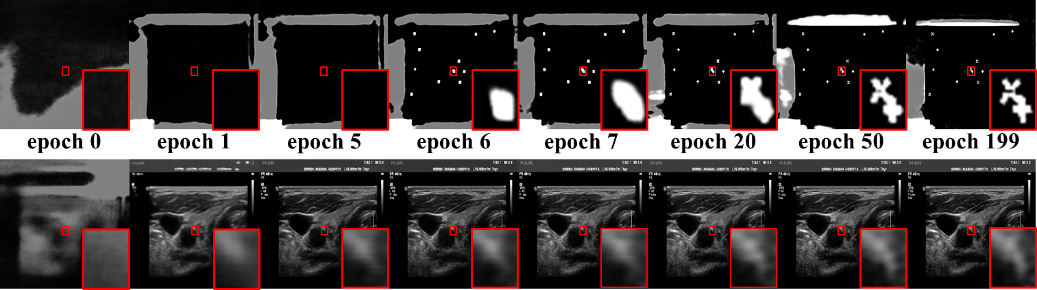
Figure 4: The learning process of the two-branch generator in several typical epochs. The first line represents the learning process of one branch for mask prediction, while the second line shows the learning process of the other branch for inpainting.

Fig. 4 shows the learning process of mask prediction and inpainting of the two-branch generator.

3.4 Ablation Study

In this section, we conduct experiments on US dataset to sort out which components of our framework contribute the most to the final performance. The original YOLOv5 + Deepfillv2 [27, 10] two-stage inpainting network is also compared as a baseline. Table 3 and Fig. 5 show Quantitative and qualitative comparisons.

Table 3: Ablation studies of individual components. “A” represents our complete model. “B” replaces the object-aware discriminator with the one in SN-PatchGAN from Deepfillv2. “C” replaces our two-branch reconstruction network with a single branch one. “D” represents a two-stage inpainting solution with YOLOv5 and Deepfillv2 trained separately.

Type	Model	PSNR$\uparrow$	SSIM$\uparrow$	MSE$\downarrow$
A	Complete Model	$\textbf{47.673}_{\pm 5.415}$	$\textbf{0.999}_{\pm 0.001}$	$\textbf{2.633}_{\pm 5.856}$
B	w/o Object-aware Discriminator	$33.283_{\pm 2.023}$	$0.984_{\pm 0.006}$	$33.948_{\pm 16.306}$
C	w/o Two-branch Reconstruction	$29.306_{\pm 2.131}$	$0.883_{\pm 0.038}$	$87.551_{\pm 52.855}$
D	Two-Stage (YOLOv5+Deepfillv2)	$43.551_{\pm 3.014}$	$0.998_{\pm 0.001}$	$4.583_{\pm 9.094}$

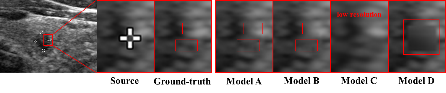
Figure 5: The qualitative comparisons of variants of the model. Our complete model “A” produces visually appealing results, supporting high-quality image completion. Model “B” appears to be losing fine texture details. Model “C” has low-quality resolution. Model “D” demonstrates a degradation in texture restoration.

Object-aware Discrimination. Our study investigates whether a discriminator based on dense object detector could enhance high-quality adversarial training. We replaced the YOLOv5-based discriminator with the one in SN-PatchGAN from Deepfillv2 (model “B” in Table 3), and observed performance degradation in all metrics, particularly in MSE and PSNR. These findings suggest some loss of fidelity in the inpainting images. Also we present visualisations in Fig. 5. Compared to model “B”, our complete model utilizes the powerful recognition capabilities of dense object detectors to identify artificial markers.

Two-branch Reconstruction Network Structure. We also compared our two-branch reconstruction network with a single branch one. The results, presented in Table 3, indicate that our complete model (model “A”) achieved superior performance compared to model “C” with a 62.67% improvement in PSNR. Additionally, as seen in Fig. 5, model “C” lost texture details while our complete model produced more visually appealing results, supporting high-quality image completion. This is because the mask prediction branch of the reconstruction network helps the model focus on marker regions in the fusion process.

Comparison with the Two-Stage Baseline. Model “D” represents a two-stage inpainting solution that utilizes separately trained YOLOv5 and Deepfillv2 models. However, this approach demonstrates a degradation in texture restoration compared to our end-to-end blind inpainting method. Our findings are supported by both quantitative and qualitative results, which confirm the effectiveness of our approach for blind inpainting.

4 Conclusion

In this work, we propose a novel blind inpainting method with a mask-free reconstruction network and an object-aware discriminator for artificial marker removal in medical images. It relaxes the restriction of specific mask input for target areas in an image. And it demonstrates the practicability of the application of using dense object detectors as discriminators. We validate our method on multiple medical image datasets such as US, EM, and MRI, which verifies that our method is effective and robust in the blind inpainting task.

Future Works. For future works, we plan to combine the diffusion models in the reconstruction network to achieve superior performance and validate the performance in large hole blind image inpainting.

References

- [1] Afonso, M.V., Sanches, J.M.R.: Blind inpainting using and total variation regularization. IEEE Transactions on Image Processing 24(7), 2239–2253 (2015)
- [2] Armanious, K., Kumar, V., Abdulatif, S., Hepp, T., Gatidis, S., Yang, B.: ipa-medgan: Inpainting of arbitrary regions in medical imaging. In: 2020 IEEE international conference on image processing (ICIP). pp. 3005–3009. IEEE (2020)
- [3] Belli, D., Hu, S., Sogancioglu, E., van Ginneken, B.: Context encoding chest x-rays. arXiv preprint arXiv:1812.00964 (2018)
- [4] Cai, N., Su, Z., Lin, Z., Wang, H., Yang, Z., Ling, B.W.K.: Blind inpainting using the fully convolutional neural network. The Visual Computer 33, 249–261 (2017)
- [5] Cao, S., Chai, W., Hao, S., Zhang, Y., Chen, H., Wang, G.: Difffashion: Reference-based fashion design with structure-aware transfer by diffusion models. arXiv preprint arXiv:2302.06826 (2023)
- [6] Currie, G., Hawk, K.E., Rohren, E., Vial, A., Klein, R.: Machine learning and deep learning in medical imaging: intelligent imaging. Journal of medical imaging and radiation sciences 50(4), 477–487 (2019)
- [7] Dong, B., Li, J., Shen, Z.: X-ray ct image reconstruction via wavelet frame based regularization and radon domain inpainting. Journal of Scientific Computing 54, 333–349 (2013)
- [8] Dong, Q., Cao, C., Fu, Y.: Incremental transformer structure enhanced image inpainting with masking positional encoding. In: Proceedings of the IEEE/CVF Conference on Computer Vision and Pattern Recognition. pp. 11358–11368 (2022)
- [9] Elharrouss, O., Almaadeed, N., Al-Maadeed, S., Akbari, Y.: Image inpainting: A review. Neural Processing Letters 51, 2007–2028 (2020)
- [10] Jocher, G., Chaurasia, A., Stoken, A., Borovec, J., NanoCode012, Kwon, Y., TaoXie, Fang, J., imyhxy, Michael, K., Lorna, V, A., Montes, D., Nadar, J., Laughing, tkianai, yxNONG, Skalski, P., Wang, Z., Hogan, A., Fati, C., Mammana, L., AlexWang1900, Patel, D., Yiwei, D., You, F., Hajek, J., Diaconu, L., Minh, M.T.: ultralytics/yolov5: v6.1 - TensorRT, TensorFlow Edge TPU and OpenVINO Export and Inference (Feb 2022). https://doi.org/10.5281/zenodo.6222936, https://doi.org/10.5281/zenodo.6222936
- [11] Li, W., Lin, Z., Zhou, K., Qi, L., Wang, Y., Jia, J.: Mat: Mask-aware transformer for large hole image inpainting. In: Proceedings of the IEEE/CVF conference on computer vision and pattern recognition. pp. 10758–10768 (2022)
- [12] Litjens, G., Toth, R., Van De Ven, W., Hoeks, C., Kerkstra, S., van Ginneken, B., Vincent, G., Guillard, G., Birbeck, N., Zhang, J., et al.: Evaluation of prostate segmentation algorithms for mri: the promise12 challenge. Medical image analysis 18(2), 359–373 (2014)
- [13] Liu, H., Wan, Z., Huang, W., Song, Y., Han, X., Liao, J.: Pd-gan: Probabilistic diverse gan for image inpainting. In: Proceedings of the IEEE/CVF Conference on Computer Vision and Pattern Recognition. pp. 9371–9381 (2021)
- [14] Liu, L., Ren, Y., Lin, Z., Zhao, Z.: Pseudo numerical methods for diffusion models on manifolds. arXiv preprint arXiv:2202.09778 (2022)
- [15] Liu, Q., Tan, Z., Chen, D., Chu, Q., Dai, X., Chen, Y., Liu, M., Yuan, L., Yu, N.: Reduce information loss in transformers for pluralistic image inpainting. In: Proceedings of the IEEE/CVF Conference on Computer Vision and Pattern Recognition. pp. 11347–11357 (2022)
- [16] Liu, Y., Pan, J., Su, Z.: Deep blind image inpainting. In: Intelligence Science and Big Data Engineering. Visual Data Engineering: 9th International Conference, IScIDE 2019, Nanjing, China, October 17–20, 2019, Proceedings, Part I 9. pp. 128–141. Springer (2019)
- [17] Lugmayr, A., Danelljan, M., Romero, A., Yu, F., Timofte, R., Van Gool, L.: Repaint: Inpainting using denoising diffusion probabilistic models. In: Proceedings of the IEEE/CVF Conference on Computer Vision and Pattern Recognition. pp. 11461–11471 (2022)
- [18] Ronneberger, O., Fischer, P., Brox, T.: U-net: Convolutional networks for biomedical image segmentation. In: Medical Image Computing and Computer-Assisted Intervention–MICCAI 2015: 18th International Conference, Munich, Germany, October 5-9, 2015, Proceedings, Part III 18. pp. 234–241. Springer (2015)
- [19] Rouzrokh, P., Khosravi, B., Faghani, S., Moassefi, M., Vahdati, S., Erickson, B.J.: Multitask brain tumor inpainting with diffusion models: A methodological report. arXiv preprint arXiv:2210.12113 (2022)
- [20] Shen, J., Zhang, C.J., Jiang, B., Chen, J., Song, J., Liu, Z., He, Z., Wong, S.Y., Fang, P.H., Ming, W.K., et al.: Artificial intelligence versus clinicians in disease diagnosis: systematic review. JMIR medical informatics 7(3), e10010 (2019)
- [21] Simonyan, K., Zisserman, A.: Very deep convolutional networks for large-scale image recognition. arXiv preprint arXiv:1409.1556 (2014)
- [22] Sirinukunwattana, K., Snead, D.R., Rajpoot, N.M.: A stochastic polygons model for glandular structures in colon histology images. IEEE transactions on medical imaging 34(11), 2366–2378 (2015)
- [23] Suvorov, R., Logacheva, E., Mashikhin, A., Remizova, A., Ashukha, A., Silvestrov, A., Kong, N., Goka, H., Park, K., Lempitsky, V.: Resolution-robust large mask inpainting with fourier convolutions. In: Proceedings of the IEEE/CVF winter conference on applications of computer vision. pp. 2149–2159 (2022)
- [24] Wang, Y., Chen, Y.C., Tao, X., Jia, J.: Vcnet: A robust approach to blind image inpainting. In: Computer Vision–ECCV 2020: 16th European Conference, Glasgow, UK, August 23–28, 2020, Proceedings, Part XXV 16. pp. 752–768. Springer (2020)
- [25] Wang, Y., Yu, J., Zhang, J.: Zero-shot image restoration using denoising diffusion null-space model. arXiv preprint arXiv:2212.00490 (2022)
- [26] Xie, J., Xu, L., Chen, E.: Image denoising and inpainting with deep neural networks. Advances in neural information processing systems 25 (2012)
- [27] Yu, J., Lin, Z., Yang, J., Shen, X., Lu, X., Huang, T.S.: Free-form image inpainting with gated convolution. In: Proceedings of the IEEE/CVF international conference on computer vision. pp. 4471–4480 (2019)
- [28] Zamir, S.W., Arora, A., Khan, S., Hayat, M., Khan, F.S., Yang, M.H., Shao, L.: Multi-stage progressive image restoration. In: Proceedings of the IEEE/CVF conference on computer vision and pattern recognition. pp. 14821–14831 (2021)
- [29] Zheng, H., Lin, Z., Lu, J., Cohen, S., Shechtman, E., Barnes, C., Zhang, J., Xu, N., Amirghodsi, S., Luo, J.: Image inpainting with cascaded modulation gan and object-aware training. In: Computer Vision–ECCV 2022: 17th European Conference, Tel Aviv, Israel, October 23–27, 2022, Proceedings, Part XVI. pp. 277–296. Springer (2022)