PoPeC: PAoI-Centric Task Offloading with Priority over Unreliable Channels

Abstract

Freshness-aware computation offloading has garnered increasing attention recently in the realm of edge computing, driven by the need to promptly obtain up-to-date information and mitigate the transmission of outdated data. However, most of the existing works assume that channels are reliable, neglecting the intrinsic fluctuations and uncertainty in wireless communication. More importantly, offloading tasks typically have diverse freshness requirements. Accommodation of various task priorities in the context of freshness-aware task scheduling and resource allocation remains an open and unresolved problem. To overcome these limitations, we cast the freshness-aware task offloading problem as a multi-priority optimization problem, considering the unreliability of wireless channels, prioritized users, and the heterogeneity of edge servers. Building upon the nonlinear fractional programming and the ADMM-Consensus method, we introduce a joint resource allocation and task offloading algorithm to solve the original problem iteratively. In addition, we devise a distributed asynchronous variant for the proposed algorithm to further enhance its communication efficiency. We rigorously analyze the performance and convergence of our approaches and conduct extensive simulations to corroborate their efficacy and superiority over the existing baselines.

I Introduction

Edge computing is an attractive computing paradigm in the era of the Artificial Internet of Things (AIoT) [1, 2]. By enabling end devices to offload computation-intensive tasks to nearby edge nodes, it is envisioned to provide real-time computing services, thereby facilitating the deployment of a wide range of intelligent applications (e.g., smart homes, smart cities, and autonomous vehicles) [3]. In these applications, it is of paramount importance to promptly access up-to-date information while mitigating the transmission of outdated and worthless data [4]. To this end, a great number of offloading solutions have been proposed to ensure timely status updates and rapid delivery of tasks from information sources, with the aim of enhancing the overall information freshness [5, 6, 7, 8, 9].

Recently, the Age of Information (AoI) and Peak Age of Information (PAoI) have been recognized as important metrics for evaluating the freshness of information, which characterize the elapsed time since the reception of a user’s most recent data packet [10]. Based on these metrics, several recent efforts have focused on AoI- or PAoI-centric computation offloading and resource allocation for efficient and concurrent transmission of freshness-sensitive information to the edge servers [7, 11, 12, 13, 9, 4, 6, 5, 8, 14, 15, 16, 17].

Unfortunately, there remain several challenges that need to be surmounted to achieve effective freshness-aware computation offloading in practice. First, many existing works assume channel homogeneity [18, 8] or perfect knowledge of channel states [9, 19], overlooking the dynamics and stochasticity of the limited wireless channels. As a result, such methods easily suffer from package loss or failure due to unreliable communication [13]. Second, computing resources on edge servers are typically constrained and heterogeneous, necessitating appropriate assignment of heterogeneous computing units to offloading tasks. More importantly, designing a prioritized offloading strategy is crucial because users may have diverse freshness requirements. For example, devices with safety-sensitive functions, such as temperature sensors in the Industrial Internet of Things and Automatic Emergency Braking (AEB) systems in autopilots, require prompt offloading and processing to meet their stringent freshness demands. Whereas, most of the existing methods struggle with measuring and handling the situations where offloading tasks possess different priorities. In light of these considerations, this work seeks to answer the key question: “How to design an efficient task offloading algorithm that can optimize the overall information freshness while effectively handling prioritized users, unreliable channels, and heterogeneous edge servers?”

To this end, we cast the freshness-aware task offloading problem as a multi-priority optimization problem, considering unreliability of wireless channels, heterogeneity of edge servers, and interdependence of multiple users with differing priorities. Given the high complexity of directly optimizing this problem, we first examine two special cases from the original problem and exploit nonlinear fractional programming to transform the problems into tractable forms, subsequently developing ADMM-Consensus-based solutions for both cases. Built upon these solutions, an iterative algorithm is devised to resolve the original problem effectively. We further discuss a distributed asynchronous variant of the proposed algorithm, capable of alleviating the overhead caused by unreliable iterations during the offloading policy acquisition process. Theoretical analysis is carried out to establish the convergence property of the proposed algorithm and demonstrate the improvement in performance brought by the multi-priority mechanism.

In a nutshell, our main contributions are summarized below.

• We consider an M/G/1 offloading system and derive the precise Peak Age of Information (PAoI) expression for each user to characterize their information freshness. Then, we formulate the freshness-aware multi-priority task offloading problem under heterogeneous edge servers and unreliable channels.

• Based on nonlinear fractional programming and the ADMM-Consensus method, we propose a joint resource allocation, service migration, and task offloading algorithm to solve the original problem effectively. We further devise a distributed asynchronous variant for the proposed algorithm to enhance its communication efficiency.

• We establish theoretical guarantees for the proposed algorithms, in terms of performance and convergence. We conduct extensive simulations, and the results show that our algorithm can significantly improve the performance over the existing methods.

The remainder of the paper is organized as follows: Section II briefly reviews the related work. Section III introduces the system model, including relevant definitions and models. In Section IV, we describe some special cases and propose algorithms to tackle the PoPeC problem. Section V proposes an asynchronous parallel algorithm to improve communication efficiency and discusses the benefits of the multi-class priority mechanism. Section VI presents the simulation results, followed by a conclusion drawn in Section VII.

II Related Work

In the realm of edge computing, a multitude of research efforts have emerged to mitigate response delays by means of task offloading strategies [20, 21, 22, 23, 24, 25, 26, 27, 28, 29, 30]. On the one hand, exploring the characteristics of channels is integral to this field. The reliability of channels has been investigated in scenarios such as real-time monitoring systems [31, 32]. However, these approaches might not adequately address the challenges posed by unstable channel conditions stemming from factors like antenna beamforming and fading [33, 34]. Moreover, while earlier studies assumed either homogeneous channels or the offloading of two separate channels with random arrivals [18, 9, 8], such assumptions fall short when dealing with the complexities of heterogeneous unreliable channels. On the other hand, one notable departure in our work is the consideration of the performance of synchronous parallel iterative algorithms in the context of unreliable channels. While many studies advocate for distributed methods to enhance efficiency, they often neglect the substantial communication costs of synchronous parallel algorithms on unreliable channels [6, 4, 5]. In contrast, we explore the potential of an asynchronous parallel algorithm to mitigate communication overheads and achieve the same performance.

Nonetheless, the sole emphasis on delay reduction may not ensure the necessary freshness of information for users, as highlighted in the works of Kosta et al. [35] and Yates et al. [10]. This has led to the development of freshness-aware methodologies, leveraging metrics such as AoI and Peak Age of Information (PAoI) [11, 12, 36, 4, 5, 6, 7, 8, 9]. Therefore, recent advancements have delved into the customization of computation offloading strategies to accommodate distinct user types and preferences [9, 5, 4, 6, 37, 38, 39, 40, 41, 42, 43]. Zou et al. [4] introduce a novel partial-index approach that accurately characterizes indexing issues in heterogeneous multi-user multi-channel systems. Their SWIM framework optimizes resource allocation using maximum weights. Sun et al. [6] propose an age-aware scheduling strategy rooted in Lyapunov optimization to cater to diverse users, providing bounds on age that comply with throughput constraints. However, many of these contributions overlook the importance of user priorities, which is vital for practical prioritized systems [9, 5, 4, 6, 37].

In contrast to prior works, which may focus on specific aspects such as channel types, reliability, or algorithmic choices, our research amalgamates these elements to address the intricate interplay of AoI optimization, edge computing, and heterogeneous channels. By investigating the challenges unique to these intersections, we contribute to a more comprehensive understanding of real-time computation offloading in dynamic environments.

III System Model

In this section, we introduce the system model, including the Mobile Edge Computing (MEC) architecture, the freshness model, and the problem formulation.

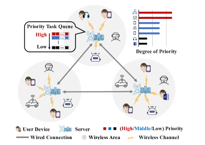
Figure 1: MEC Architecture with Unreliable Channles and Priority Users.

III-A MEC Architecture

As shown in Fig.1, we consider a wireless network system consisting of a set of $M$ mobile edge servers (denoted by $\mathcal{M}$). Each server $m\in\mathcal{M}$ serves a set of $N_{m}$ users ($\mathcal{N}_{m}$), and each user $n\in\mathcal{N}$ can offload their tasks to the corresponding server $m_{n}$ via a limited number of wireless channels (denoted by $\mathcal{C}\doteq\{1,\dots,C\}$). Considering the effects of frequency-selective fading [4], we define $p_{n,c}$ as the probability of a successful transmission from user $n$ through channel $c$ to server $m_{n}$. In this context, users have (potentially) varying offloading priorities, represented as $\Delta\doteq\{1,2,\dots,\delta_{\mathrm{max}}\}$. Let $\mathcal{N}^{\delta}_{m}$ denote the set of users that are prioritized as $\delta\in\Delta$ and served by server $m$, which satisfies $\bigcup_{m\in\mathcal{M}}\bigcup_{\delta\in\Delta}\mathcal{N}^{\delta}_{m}=\bigcup_{m\in\mathcal{M}}\mathcal{N}_{m}=\mathcal{N}$. We represent $\mathcal{N}^{\delta}\doteq\bigcup_{m\in\mathcal{M}}\mathcal{N}^{\delta}_{m}$ as the set of users with priority $\delta$ across all servers. To simplify notation, we denote the priority of user $n$ as $\delta(n)$ and the set of users with the same or higher priority as $\Delta(\delta(n))$. Particularly, we distinguish user-side and server-side variables using the superscripts ‘u’ and ‘s’, respectively. For clarity, we summarize the key notations in Table I.

TABLE I: Key Notations

Notation	Definition
$n$, $c$, $m$, $\delta$	indexes of users, channels, servers, and priority
$u$, $s$	superscripts of user-side and server-side variables
$\lambda_{n}$, $\mu_{n}$	expected arrival and service rates of $n$’s offloaded tasks
$p_{n,c}$	probability of a successful update from user $n$ to channel $c$
$y_{m}$	optimal migration decision of server $m$
$\eta^{u}_{n,c}$	probability of tasks offloading from user $n$ to channel $c$
$\eta^{s}_{m,m^{\prime}}$	proportion of tasks delivered from server $m$ to server $m^{\prime}$
$p^{\mathrm{syn}}$, $p^{\mathrm{asyn}}$	probability of a successful (a)synchronous update
$\Gamma^{\mathrm{syn}}$, $\Gamma^{\mathrm{asyn}}$	number of iterations of (a)synchronous algorithms
$T_{n}$, $I_{n}$, $W_{n}$, $Y_{n}$	user $n$’s transmission time, arrival interval, waiting time, and processing time
$A_{n}$	PAoI of user $n$’s message
$\epsilon^{\mathrm{ck}}$, $\epsilon^{\mathrm{ac}}$	stop criteria for iterations CheckPointing Algorithm (NFP) and ADMM-Consensus Algorithm (NAC/ANAC)

III-A1 Task Offloading

The computational tasks of each user arrive according to a Poisson process with an expected arrival rate of $\lambda_{n}$. We denote the probability of user $n$ accessing channel $c$ as $\eta^{u}_{n,c}$, which satisfies

$$0\leq\eta^{u}_{n,c}\leq 1,\quad\forall n\in\mathcal{N},~{}c\in\mathcal{C}.$$ (1)

Clearly, the number of tasks offloaded by user $n$ through channel $c$ also adheres to a Poisson progress with an expected value of $\eta^{u}_{n,c}\lambda_{n}$. Given the fact that the number of offloaded tasks by user $n$ can not exceed that generated by the same user, we have

$$\sum_{c\in\mathcal{C}}\eta^{u}_{n,c}\leq 1,\quad\forall n\in\mathcal{N}.$$ (2)

The inequality in Eq. (2) holds from the fact that users may discard outdated tasks due to congestion in the channel, or a need to prioritize more urgent tasks [44].

Edge servers are connected to each other via a wired network and can collaborate to execute offloaded tasks by assigning a portion of tasks from one server to another. We represent $\eta^{s}_{m,m^{\prime}}$ as the proportion of tasks delivered from server $m$ to server $m^{\prime}$, which satisfies

$$0\leq\eta^{s}_{m,m^{\prime}}\leq 1, \quad\forall m,m^{\prime}\in\mathcal{M},$$ (3)

$$\sum_{m^{\prime}\in\mathcal{M}}\eta^{s}_{m,m^{\prime}}=1, \quad\forall m\in\mathcal{M}.$$ (4)

Accordingly, the number of computational tasks with priority $\delta$ delivered from server $m$ to $m^{\prime}$ can be expressed as $\eta^{s}_{m,m^{\prime}}\lambda^{s}_{\delta,m}$, where

$$\lambda^{s}_{\delta,m}\doteq\sum_{n\in\mathcal{N}^{\delta}_{m}}\sum_{c\in\mathcal{C}}p_{n,c}\lambda_{n,c}.$$ (5)

$\lambda^{s}_{\delta,m}$ denotes the total number of received tasks prioritized as $\delta$ at server $m$. Since the total number of tasks arrived at each server cannot exceed its maximum capacity (denoted by $\lambda^{s,\mathrm{max}}_{m}$), we have

$$\sum_{\delta\in\Delta}\sum_{m^{\prime}\in\mathcal{M}}\eta^{s}_{m^{\prime},m}\lambda^{s}_{\delta,m^{\prime}}\leq\lambda^{s,\mathrm{max}}_{m},\quad\forall m\in\mathcal{M}.$$ (6)

III-A2 Transmission Model

We assume that the transmission process of the multiple access channel follows the M/M/1 queuing model, as in [45, 46].^, We denote the task arrival rate of channel $c$ as $\lambda_{c}\doteq\sum_{n\in\mathcal{N}}\eta^{u}_{n,c}\lambda_{n}$, i.e., the sum of the offloading arrival rates of all users accessing this channel. Meanwhile, $r_{c}$ stands for the communication for transmission rate through channel $c$, and $S$ denotes the package size. As the currently achievable wireless communication rate approaches the Shannon limit [47], the transmission rate can be expressed as $r_{c}=B_{c}\log\bigl{(}R_{c}+1\bigr{)}$, where $B_{c}$ and $R_{c}$ are the bandwidth and the signal-to-noise ratio of channel $c$, respectively. Thus, if user $n$ accesses channel $c$, the expected transmission time can be expressed by

$$T^{\mathrm{tr}}_{n,c}=\left\{\begin{array}[]{ll}\frac{1}{r_{c}/S-\lambda_{c}}+t_{n,c},&\quad\frac{r_{c}}{S}-\lambda_{c}>0,\\ \infty,&\quad\mathrm{otherwise},\end{array}\right.$$ (7)

where $\frac{1}{r_{c}/S-\lambda_{c}}$ is the channel contention time, and $t_{n,c}$ is the constant end-to-end propagation delay of the offloading tasks. The propagation delay, in a short time slice, is calculated by dividing the distance between the user and the server ($d_{n,c}$) by the speed at which the wireless signal propagates through the air ($v_{c}$), i.e., $t_{n,c}=\frac{d_{n,c}}{v_{c}}$ [48]. As in [49], since MEC servers are linked via wired core networks, we assume that the end-to-end propagation delay between servers $m$ and $m^{\prime}$ is constant, denoted by $t^{\mathrm{tr}}_{m,m^{\prime}}$.

III-B Limited Capacity Model with Confidence Evaluation

To meet the requirements of real-time response, we consider the limited channel capacity/computation models with confidence, which enable real-time estimation and the control of system stability [5, 50].

III-B1 Channel Capacity

Denote the capacity of channel $c$ as $M_{c}^{\mathrm{max}}$. Based on the properties of the cumulative distribution function of the Poisson distribution [51], we introduce the following constraint to ensure that each channel is conflict-free with confidence level $1-\alpha$ [50, 5]:

$$\frac{z^{2}_{1}}{2}+z_{2}\cdot\left(\sum_{n\in\mathcal{N}}\eta^{u}_{n,c}\lambda_{n}+\frac{z^{2}_{2}}{4}\right)^{\frac{1}{2}}+\sum_{n\in\mathcal{N}}\eta^{u}_{n,c}\lambda_{n}\leq M_{c}^{\mathrm{max}}.$$ (8)

Here, $z_{1}\doteq(\alpha/2-\lambda^{\mathrm{chl}}_{c})/\sqrt{\lambda^{\mathrm{chl}}_{c}}$ and $z_{2}\doteq(1-\alpha/2-\lambda^{\mathrm{chl}}_{c})/\sqrt{\lambda^{\mathrm{chl}}_{c}}$ are two statistics standardized from a normal distribution, where $\lambda^{\mathrm{chl}}_{c}\doteq\sum_{n\in\mathcal{N}}\eta^{u}_{n,c}\lambda_{n}$ represents the total number of tasks transmitted through channel $c$.

$$\mathbb{E}[W^{p}_{n}]=\, \frac{\frac{1}{2}\sum_{\delta\in\Delta}\sum_{n^{\prime}\in\mathcal{N}^{\delta}}\sum_{c\in\mathcal{C}}p_{n^{\prime},c}\eta^{u}_{n^{\prime},c}\lambda_{n^{\prime}}\nu_{n^{\prime}}}{\left(1-\sum_{\delta\in\Delta(\delta(n))}\sum_{n^{\prime}\in\mathcal{N}^{\delta}}\sum_{c\in\mathcal{C}}p_{n^{\prime},c}\frac{\eta^{u}_{n^{\prime},c}\lambda_{n^{\prime}}}{\mu_{n^{\prime}}}\right)\left(1-\sum_{\delta\in\Delta(\delta(n)-1)}\sum_{n^{\prime}\in\mathcal{N}^{\delta}}\sum_{c\in\mathcal{C}}p_{n^{\prime},c}\frac{\lambda_{n^{\prime},c}}{\mu_{n^{\prime}}}\right)}$$ (9)

$$\pi_{n,m}(\bm{\eta}^{s})\doteq\, \frac{\sum_{\delta\in\Delta}\eta^{s}_{m_{n},m}\lambda^{s}_{\delta,m_{n}}}{\sum_{\delta\in\Delta}\sum_{m^{\prime}\in\mathcal{M}}\eta^{s}_{m_{n},m^{\prime}}\lambda^{s}_{\delta,m_{n}}}\cdot\left(t^{\mathrm{tr}}_{m_{n},m}+\frac{1}{\mu_{n,m}}+\frac{1}{1-\sum_{\delta\in{\Delta(\delta(n))}}\sum_{m^{\prime}\in\mathcal{M}}\eta^{s}_{m^{\prime},m}\lambda^{s}_{\delta,m^{\prime}}\frac{1}{\mu_{n,m}}}\right.$$

$$\left.\cdot\frac{\frac{1}{2}\sum_{\delta\in\Delta}\sum_{m^{\prime}\in\mathcal{M}}\eta^{s}_{m^{\prime},m}\lambda^{s}_{\delta,m^{\prime}}\nu_{n,m}}{1-\sum_{\delta\in{\Delta(\delta(n)-1)}}\sum_{m^{\prime}\in\mathcal{M}}\eta^{s}_{m^{\prime},m}\lambda^{s}_{\delta,m^{\prime}}\frac{1}{\mu_{n,m}}}\right)$$ (10)

 

III-B2 Computation Capacity

Due to the fluctuation in servers’ available computing capacities, we assume that server $m$’s processing time for user $n$’s tasks follows a general distribution with mean $1/\mu_{n,m}$ and second moment $\nu_{n,m}$ [38]. To simplify notations, we use $1/\mu_{n}$ and $\nu_{n}$ to represent $1/\mu_{n,m_{n}}$ and $\nu_{n,m_{n}}$, respectively. To ensure each task is executed with a confidence level of $1-\beta$, we impose the following constraint:

$$\begin{split}\frac{z^{2}_{3}}{2}&+z_{4}\cdot\left(\sum_{n\in\mathcal{N}}\sum_{c\in\mathcal{C}}p_{n,c}\cdot\frac{\eta^{u}_{n,c}\lambda_{n}}{\mu_{n}}+\frac{z^{2}_{4}}{4}\right)^{\frac{1}{2}}\\ &+\sum_{n\in\mathcal{N}}\sum_{c\in\mathcal{C}}p_{n,c}\cdot\frac{\eta^{u}_{n,c}\lambda_{n}}{\mu_{n}}<1,\end{split}$$ (11)

where $z_{3}\doteq(\beta/2-\lambda^{\mathrm{comp}}_{c})/\sqrt{\lambda^{\mathrm{comp}}_{c}}$ and $z_{4}\doteq(1-\beta/2-\lambda^{\mathrm{comp}}_{c})/\sqrt{\lambda^{\mathrm{comp}}_{c}}$ are two statistics standardized from a normal distribution, with $\lambda^{\mathrm{comp}}\doteq\sum_{n\in\mathcal{N}}\sum_{c\in\mathcal{C}}p_{n,c}\eta^{u}_{n,c}\lambda_{n}/\mu_{n}$ the total number of tasks arriving at server $m(n)$.

III-C Freshness Model and Problem Formulation

We characterize the freshness of information using the PAoI metric. Specifically, the PAoI of user $n$’s message, denoted by $A_{n}$, is determined by four key factors: transmission time $T_{n}$, arrival interval $I_{n}$, waiting time $W_{n}$, and processing time $Y_{n}$ [4], i.e.,

$$\mathbb{E}[A_{n}] =\mathbb{E}[T_{n}]+\mathbb{E}[I_{n}]+\mathbb{E}[W_{n}]+\mathbb{E}[Y_{n}],$$ (12)

with $\mathbb{E}[I_{n}]=1/\sum_{c\in\mathcal{C}}p_{n,c}\eta^{u}_{n,c}\lambda_{n}$ and $\mathbb{E}[T_{n}]=\sum_{c\in\mathcal{C}}\eta^{u}_{n,c}T^{\mathrm{tr}}_{n,c}$. The expressions of $\mathbb{E}[W_{n}]$ and $\mathbb{E}[Y_{n}]$ are contingent upon the way in which user $n$’s tasks are executed. To derive the precise expressions, we use binary variable $y_{m}$ to denote the migration decision of server $m$, i.e.,

$$y_{m}\in\{0,1\},\quad\forall m\in\mathcal{M}.$$ (13)

If $y_{m}$ comes to 0, server $m$ executes its tasks locally; otherwise, it resorts to the other servers for collaboration. In a slightly abusive notation, we use the superscript ‘p’ to represent the case when $y_{m}=0$ and the superscript ‘s’ to represent the case when $y_{m}=1$. Thus, when $y_{m_{n}}=0$, $\mathbb{E}[Y^{p}_{n}]=1/\mu_{n}$, and $\mathbb{E}[W^{p}_{n}]$ can be expressed in Eq. (9) from the M/G/1 queuing model with FCFS (see Appendix A of technical report [52] for more details). When $y_{m_{n}}=1$, according to Little’s Law, we can obtain

$$\mathbb{E}[W^{s}_{n}]+\mathbb{E}[Y^{s}_{n}]=\sum_{m\in\mathcal{M}}\pi_{n,m}(\bm{\eta}^{s}),$$ (14)

where $\bm{\eta}^{s}\doteq\{\eta^{s}_{m,m^{\prime}}\}_{m,m^{\prime}\in\mathcal{M}}$, and $\pi_{n,m}(\bm{\eta}^{s})$ is defined in Eq. (10). Based on this, the expected PAoI of user $n$ can be specified as follows:

$$\mathbb{E}[A_{n}]=(1-y_{m_{n}})\cdot\mathbb{E}[A_{n}|y_{m_{n}}=0]+y_{m_{n}}\cdot\mathbb{E}[A_{n}|y_{m_{n}}=1].$$ (15)

Given the aforementioned constraints, our objective is to find the optimal offloading decision for users and the collaboration decision for servers to minimize the average expected PAoI across all users. We cast the problem as the PAoI-Centric Task Offloading with Priority over Unreliable Channels (PoPeC):

$$\begin{split}&\textbf{(PoPeC)}~{}\mathop{\min}_{\bm{\eta}^{u},\bm{\eta}^{s},\bm{y}}\frac{1}{N}\sum_{n\in\mathcal{N}}\mathbb{E}[A_{n}],\\ &\qquad\quad\text{s.t.}~{}\eqref{eq:c1}\textrm{--}\eqref{eq:c4a},\eqref{eq:c7a},\eqref{eq:c8a},\eqref{eq:c-y},\end{split}$$ (16)

with $\bm{\eta}^{u}\doteq\{\eta^{u}_{n,c}\}_{n\in\mathcal{N},c\in\mathcal{C}}$ the offloading decision, and $\bm{\eta}^{s}\doteq\{\eta^{s}_{m,m^{\prime}}\}_{m,m^{\prime}\in\mathcal{M}}$ along with $\bm{y}\doteq\{y_{m}\}_{m\in\mathcal{M}}$ the collaboration decision.

IV PoPeC: PAoI-Centric Task Offloading with Priority over Unreliable Channels

In light of the challenges in directly addressing the offloading problem, this section begins by examining two special cases – priority-free and multi-priority task scheduling with no server collaboration. Building on the insights gained from these solutions, we subsequently devise an effective and efficient algorithm for optimizing the original problem.

IV-A Priority-Free Task Scheduling

IV-A1 Problem Transformation

We first focus on a special case in which all tasks are of the same type and do not possess any priority distinctions, i.e., the problem of offloading to the local servers. To solve this problem, the first step is to derive the expression of the expected PAoI for each user in this context. Recall that each user’s task arrivals follow a Poisson distribution, and task execution times follow a general distribution. We re-evaluate the waiting time based on Eq. (9) as follows:

$$\mathbb{E}[W_{n}]=\frac{\sum_{n\in\mathcal{N}}\sum_{c\in\mathcal{C}}p_{n,c}\eta^{u}_{n,c}\lambda_{n}\nu_{n}}{2\cdot\left(1-\sum_{n\in\mathcal{N}}\sum_{c\in\mathcal{C}}p_{n,c}\cdot\frac{\eta^{u}_{n,c}\lambda_{n}}{\mu_{n}}\right)}.$$ (17)

We introduce an auxiliary variable, $\hat{t}^{\mathrm{tr}}_{n}>0$, to represent the upper bound of user $n$’s transmission time through all the available channels, i.e.

$$\hat{t}^{\mathrm{tr}}_{n}\geq T^{\mathrm{tr}}_{n,c},\quad\forall c\in\mathcal{C}.$$ (18)

Akin to [54, 55], we transform the original problem into the following tractable form, i.e., optimizing a tight upper bound of user $n$’s expected PAoI:

(P1) $$\mathop{\min}_{\hat{t}^{\mathrm{tr}}_{n},\bm{\eta}^{u}}\frac{1}{N}\sum_{n\in\mathcal{N}}f_{n}(\hat{t}^{\mathrm{tr}}_{n},\bm{\eta}^{u}),$$ (19)

s.t. $$~{}\eqref{eq:c1},\eqref{eq:c2},\eqref{eq:c7a},\eqref{eq:c8a},\eqref{eq:c6}.$$

$f_{n}(\hat{t}^{\mathrm{tr}}_{n},\bm{\eta}^{u})$ is defined as:

$$f_{n}(\hat{t}^{\mathrm{tr}}_{n},\bm{\eta}^{u})\doteq\, \hat{t}^{\mathrm{tr}}+\frac{1}{\Psi_{n}(\bm{\eta}^{u})}+\frac{\upsilon_{n}(\bm{\eta}^{u})}{\phi_{n}(\bm{\eta}^{u})}+\frac{1}{\mu},$$ (20)

where we represent $\upsilon_{n}(\bm{\eta}^{u})\doteq\frac{1}{2}\sum_{n^{\prime}\in\mathcal{N}}\sum_{c\in\mathcal{C}}p_{n^{\prime},c}\cdot\eta^{u}_{n^{\prime},c}\lambda_{n^{\prime}}\nu$, $\phi_{n}(\bm{\eta}^{u})\doteq 1-\sum_{n^{\prime}\in\mathcal{N}}\sum_{c\in\mathcal{C}}p_{n^{\prime},c}\cdot\eta^{u}_{n^{\prime},c}\lambda_{n^{\prime}}/\mu$, and $\Psi_{n}(\bm{\eta}^{u})\doteq\sum_{c\in\mathcal{C}}p_{n,c}\eta^{u}_{n,c}\lambda_{n}$.

In line with the principles of min-max optimization, we can enhance the overall communication efficiency across all channels by focusing our efforts on minimizing $\hat{t}^{\mathrm{tr}}_{n}$ rather than $\mathbb{E}[T_{n}]$. This strategic shift not only aligns with our objective of improving performance but also bolsters the resilience and robustness of our proposed solution.

Eq. (8) and Eq. (11) suggest that P1 is a non-convex problem. To identify well-structured solutions, we transform these constraints into equivalent convex ones.

Lemma 1.

In Problem P1, Constraints (8) and (11) are equivalent to following Constraints (21) and (22) respectively:

$$\sum_{n\in\mathcal{N}}\eta^{u}_{n,c}\lambda_{n}\leq M_{c}^{\mathrm{max}}+\frac{z^{2}_{2}}{2}-\frac{z^{2}_{1}}{2}-z_{2}\cdot\left(M_{c}^{\mathrm{max}}+\frac{z^{2}_{2}}{2}-\frac{z^{2}_{1}}{2}\right)^{\frac{1}{2}},$$ (21)

$$\sum_{n\in\mathcal{N}}\sum_{c\in\mathcal{C}}p_{n,c}\frac{\eta^{u}_{n,c}\lambda_{n}}{\mu_{n}}\leq 1+\frac{z^{2}_{4}}{2}-\frac{z^{2}_{3}}{2}-z_{4}\cdot\left(1+\frac{z^{2}_{4}}{2}-\frac{z^{2}_{3}}{2}\right).$$ (22)

Proof.

The detailed proof can be found in Appendix B of technical report [52]. ∎

According to Lemma 1, Constraints (21) and (22) restrict the decision variables to convex sets, and hence, Problem P1 can be rewritten as:

(P1-1) $$\mathop{\min}_{\hat{t}^{\mathrm{tr}}_{n},\bm{\eta}^{u}}\frac{1}{N}\sum_{n\in\mathcal{N}}f_{n}(\hat{t}^{\mathrm{tr}}_{n},\bm{\eta}^{u}),$$ (23)

s.t. $$~{}\eqref{eq:c1},\eqref{eq:c2},\eqref{eq:c6},\eqref{eq:c7b},\eqref{eq:c8b}.$$

Building on the above transformation, we can obtain the following property.

Theorem 1.

Problem P1-1 is a convex problem.

Proof.

It is easy to see that the constraints of P1-1 are convex because they are affine sets. The convexity of all sub-functions is proven in Appendix C of technical report [52]. ∎

Based on the convexity of Problem P1-1, we can employ the ADMM technique to solve this problem, detailed in the following section.

IV-A2 Problem Decomposition and Solving

We define an auxiliary function, $g_{n}(\bm{x})$, as follows:

$$g_{n}(\bm{x})\doteq\left\{\begin{array}[]{ll}\hat{t}^{\mathrm{tr}}+\frac{1}{\Psi_{n}(\bm{\eta}^{u})}+\frac{\upsilon_{n}(\bm{\eta}^{u})}{\phi_{n}(\bm{\eta}^{u})}+\frac{1}{\mu},&\bm{x}\in\Omega,\\ \infty,&\text{otherwise.}\end{array}\right.$$ (26)

where $\bm{x}\doteq\{\hat{t}^{\mathrm{tr}},\bm{\eta}^{u}\}$, and $\Omega\doteq\{\bm{x}|\eqref{eq:c1},\eqref{eq:c2},\eqref{eq:c6},\eqref{eq:c7b},\eqref{eq:c8b}\}$ is the feasible set of Problem P1-1.

P1-1 is equivalent to the following consensus problem:

$$\textbf{(P1-2)}~{}\mathop{\min}_{\{\bm{x}_{n}\}}~{}~{} \sum_{n\in\mathcal{N}}g_{n}(\bm{x}_{n}),$$ (27)

s.t. $$~{}\bm{x}_{n}=\bm{x}_{o}.$$ (28)

According to Theorem 1, it is clear that the well-known ADMM-Consensus algorithm can be used to obtain the optimal solution of Problem P1-2[56] (For more details, please refer to Appendix D of technical report [52]).

IV-B Multi-Priority Task Scheduling

IV-B1 Problem Transformation with Nonlinear Fractional Programming

Different from priority-free task scheduling in the previous section, we delve deeper into the multi-priority task scheduling problem in this section. In this case, according to the priorities of received tasks, servers will execute the tasks with higher priorities more promptly. Since the multi-priority task scheduling, in this case, is NP-hard (please refer to Appendix M of technical report [52] for the proof), similar to Problem P1, we minimize a tight upper bound for the average expected PAoI of multi-priority users:

(P2) $$\mathop{\min}_{\bm{x}}\frac{1}{N}\sum_{n\in\mathcal{N}}f^{p}_{n}(\bm{x}),$$ (29)

s.t. $$~{}\eqref{eq:c1},\eqref{eq:c2},\eqref{eq:c7a},\eqref{eq:c8a},\eqref{eq:c6},$$

where $f^{p}_{n}(\bm{x})=\hat{t}^{\mathrm{tr}}+\frac{1}{\mu_{n}}+\frac{1}{\Psi_{n}(\bm{x})}+\frac{\Upsilon(\bm{x})}{\Phi_{\delta(n)}(\bm{x})\Phi_{\delta(n)-1}(\bm{x})}$ is the upper bound of $\mathbb{E}[A_{n}]$, $\bm{x}=\{\hat{t}^{\mathrm{tr}},\bm{\eta}^{u}\}$ denotes the decision variables, $\Phi_{\delta(n)}(\bm{x})=1-\sum_{\delta\in\Delta(\delta(n))}\sum_{n^{\prime}\in\mathcal{N}^{\delta}}\sum_{c\in\mathcal{C}}p_{n^{\prime},c}\eta^{u}_{n^{\prime},c}\lambda_{n^{\prime}}/\mu_{n^{\prime}}$, $\Upsilon(\bm{x})=\frac{1}{2}\sum_{\delta\in\Delta}\sum_{n^{\prime}\in\mathcal{N}^{\delta}}\sum_{c\in\mathcal{C}}p_{n^{\prime},c}\eta^{u}_{n^{\prime},c}\lambda_{n^{\prime}}\nu_{n^{\prime}}$, and $\Psi_{n}(\bm{x})=\sum_{c\in\mathcal{C}}p_{n,c}\eta^{u}_{n,c}\lambda_{n}$. To obtain the effective offloading decision in this case, we next transform the original problem and decouple users’ offloading decisions.

First, we define $\theta_{n}\doteq f^{p,u}_{n}(\bm{x}_{n})/f^{p,l}_{n}(\bm{x}_{n})=f^{p}_{n}(\bm{x}_{n})-1/\mu_{n}$ and write

$$\mathop{\min}_{\bm{\theta}}\sum_{n\in\mathcal{N}}\theta_{n}=\mathop{\min}_{\bm{x}}\sum_{n\in\mathcal{N}}\frac{f^{p,u}_{n}(\bm{x}_{n})}{f^{p,l}_{n}(\bm{x}_{n})}=\sum_{n\in\mathcal{N}}\frac{f^{p,u}_{n}(\bm{x}_{n}^{*})}{f^{p,l}_{n}(\bm{x}_{n}^{*})},$$ (30)

where $\bm{x}_{n}^{*}$ is the optimal solution and $f^{p,u}_{n},f^{p,l}_{n}$ are denoted by

$$f^{p,u}_{n}(\bm{x}_{n})=\; \Phi_{\delta(n)}(\bm{x}_{n})\Phi_{\delta(n)-1}(\bm{x}_{n})+\Upsilon(\bm{x}_{n})\Psi_{n}(\bm{x}_{n})$$

$$+\hat{t}^{\mathrm{tr}}\Psi_{n}(\bm{x}_{n})\Phi_{\delta(n)}(\bm{x}_{n})\Phi_{\delta(n)-1}(\bm{x}_{n}),$$ (31)

$$f^{p,l}_{n}(\bm{x}_{n})=\; \Psi_{n}(\bm{x}_{n})\Phi_{\delta(n)}(\bm{x}_{n})\Phi_{\delta(n)-1}(\bm{x}_{n}).$$ (32)

Proposition 1.

Problem P2 can be recast into an equivalent problem as follows:

$$\begin{split}\textbf{{(P2-1)}}~{}&\mathop{\min}_{\{\bm{x}_{n}\}}\sum_{n\in\mathcal{N}}f^{p,u}_{n}(\bm{x}_{n})-\theta^{*}_{n}f^{p,l}_{n}(\bm{x}_{n}),\\ \text{s.t.}&~{}~{}\eqref{eq:c1},\eqref{eq:c2},\eqref{eq:c6},\eqref{eq:c7b},\eqref{eq:c8b},\end{split}$$ (33)

where $\theta^{*}_{n}$ is the minimum value of $f^{p,u}_{n}(\bm{x}_{n})/f^{p,l}_{n}(\bm{x}_{n})$ with regard to $\bm{x}_{n}$.

Proof.

The detailed proof can be found in Appendix E of technical report [52]. ∎

Proposition 1 demonstrates that problem transformation can be employed to deal with the nonlinear fractional programming problem P2-1. Hence, we can use the iterative Dinkelbach techniques [57], outlined in Algorithm 1, to solve the transformed problem. Algorithm 1 updates the value of $\tilde{\theta}_{n}$ in each iteration based on the current $\tilde{\bm{x}}^{k}_{n}$, i.e.,

$$\tilde{\theta}^{k+1}_{n}=\frac{f^{p,u}_{n}(\tilde{\bm{x}}^{k+1}_{n})}{f^{p,l}_{n}(\tilde{\bm{x}}^{k+1}_{n}))}.$$ (34)

This process continues until:

$$f^{p,u}_{n}(\tilde{\bm{x}}^{k+1}_{n})-\tilde{\theta}^{k}_{n}f^{p,l}_{n}(\tilde{\bm{x}}^{k+1}_{n}))>\epsilon^{\mathrm{ck}},$$ (35)

where $\epsilon^{\mathrm{ck}}$ represents the stop criteria for iterations.

// CheckPointing Algorithm - NFP

Input: $\epsilon^{\mathrm{ck}}$, $\{\tilde{\theta}^{0}_{n}\}$, $k$

1 for $n=1$ to $N$ do

2       Convergence = False

3       while Convergence = False do

4             Apply Algorithm 2 or 4 with $\tilde{\bm{x}}^{k}_{n}$ and $\tilde{\theta}^{k}_{n}$ to obtain the solution $\tilde{\bm{x}}^{k+1}_{n}$

5             if $f^{p,u}_{n}(\tilde{\bm{x}}^{k+1}_{n})-\tilde{\theta}^{k}_{n}f^{p,l}_{n}(\tilde{\bm{x}}^{k+1}_{n}))>\epsilon^{\mathrm{ck}}$ then

6                   Select $\tilde{\theta}^{k+1}_{n}=\frac{f^{p,u}_{n}(\tilde{\bm{x}}^{k+1}_{n})}{f^{p,l}_{n}(\tilde{\bm{x}}^{k+1}_{n}))}$

7                   Convergence = True

8            else

9                  Convergence = False

10             end if

11            Update $s=s+1$

12            

13       end while

14      Select $\bm{x}^{p,*}_{n}=\tilde{\bm{x}}^{k}_{n}$

15       Select $\theta^{p,*}_{n}=\tilde{\theta}^{k}_{n}$

16       Calculate PAoI according to Eq. (29)

       Output: $\bm{x}^{p,*}_{n}$ and PAoI

17      

18 end for

Algorithm 1 Nonlinear fractional programming based on ADMM-Consensus (NFPA)

IV-B2 ADMM-Consensus Based Solution

The procedure mentioned above can be considered as a checkpointing algorithm. We employ non-convex ADMM-Consensus methods to determine the new value of $\{\bm{x}_{n}\}$. Analogous to section IV-A, the consensus problem for P2-1 can be expressed as:

$$\begin{split}\textbf{(P2-2)}~{}\mathop{\min}_{\{\bm{x}_{n}\}}~{}~{}&\sum_{n\in\mathcal{N}}g^{p}_{n}(\bm{x}_{n}),\\ \text{s.t.}&~{}\bm{x}_{n}=\bm{x}_{o},\end{split}$$ (36)

where

$$g^{p}_{n}(\bm{x}_{n})=\left\{\begin{array}[]{ll}f^{p,u}_{n}(\bm{x}_{n})-\theta^{*}_{n}f^{p,l}_{n}(\bm{x}_{n}),&\bm{x}\in\Omega,\\ \infty,&\text{otherwise.}\end{array}\right.$$ (39)

The augmented Lagrangian for Problem P2-2 can be expressed as:

$$L^{p}(\{\bm{x}_{n}\},\bm{x}_{o},\{\bm{\sigma}_{n}\})=\sum_{n\in\mathcal{N}}L^{p}_{n}(\bm{x}_{n},\bm{x}_{o},\bm{\sigma}_{n})$$

$$=\sum_{n\in\mathcal{N}}\left(g^{p}_{n}(\bm{x}_{n})+\langle\bm{\sigma}_{n},\bm{x}_{n}-\bm{x}_{o}\rangle+\frac{\rho_{n}}{2}\|\bm{x}_{n}-\bm{x}_{o}\|^{2}_{2}\right),$$ (40)

where $\rho_{n}$ is a positive penalty parameter with respect to Problem P2-2. Based on the non-convex ADMM-Consensus algorithm, we update the variables in each iteration $t$ as follows:

$$\bm{x}^{t+1}_{n} =\arg\min_{\bm{x}_{n}}L^{p}_{n}(\{\bm{x}_{n}\},\bm{x}^{t}_{o},\{\bm{\sigma}^{t}_{n}\}),$$ (41)

$$\bm{x}^{t+1}_{o} =\frac{\sum_{n\in\mathcal{N}}(\rho_{n}\bm{x}^{t+1}_{n}+\sigma^{t}_{n})}{\sum_{n\in\mathcal{N}}\rho_{n}},$$ (42)

$$\sigma^{t+1}_{n} =\sigma^{t}_{n}+\rho_{n}(\bm{x}^{t+1}_{n}-\bm{x}^{t+1}_{o}).$$ (43)

The premise that the iterative update can converge is that the function $g^{p}_{n}$ is Lipschitz continuous.

Proposition 2.

The first-order derivative of $g^{p}_{n}$ is Lipschitz continuous with constant $\ell_{n}$, which is defined as

$$\ell_{n}=\frac{\lambda^{2}_{max}}{\mu^{2}_{\mathrm{min}}}\Big{(}\sum_{n_{1}\in\mathcal{N}}\frac{\nu_{n}}{2\mu_{n}\mu_{n_{1}}}+(1+\theta^{*}_{n}\frac{\nu_{n}}{2\mu_{n}})|\mathcal{N}_{1}|+\theta^{*}_{n}\frac{\nu_{n}}{2\mu_{n}}|\mathcal{N}_{2}|\Big{)},$$ (44)

where $\mu_{\mathrm{min}}=\mathop{\min}_{n}\{\mu_{n}\}$, $\lambda_{max}=\mathop{\max}_{n}\lambda_{n}$, $\mathcal{N}_{1}=\{\mathcal{N}^{\delta}|\delta<\delta(n)\}\bigcup\{n\}$, $\mathcal{N}_{2}=\{\mathcal{N}^{\delta}|\delta\leq\delta(n)\}$.

Proof.

The detailed proof can be found in Appendix F of technical report [52]. ∎

According to Proposition 2, we adopt the non-convex ADMM-Consensus method to solve Problem P2-2, with given $\left(\{\bm{x}^{0}_{n}\},\{\theta^{*}_{n}\}\right)$ (as outlined in Algorithm 1).

Input: $\epsilon^{\mathrm{ac}}$, $t$ and $\left(\{\bm{x}^{0}_{n}\},\{\theta^{*}_{n}\}\right)$ from Algorithm 1

// ADMM-Consensus Algorithm

1 do

2       Calculate $\bm{x}^{t+1}_{o}$ in MEC, according to Eq. (42)

3       Calculate $\bm{x}^{t+1}_{n}$ in user, simultaneously according to Eq. (41)

4       Calculate $\sigma^{t+1}_{n}$ in user, simultaneously according to Eq. (43)

5       Update $t=t+1$

6      

7while $\eta\left(\bm{x}^{t},\bm{\sigma}^{t}\right)\geq\epsilon^{\mathrm{ac}}$;

Output: $\bm{x}^{t}_{n}$

Algorithm 2 Non-Convex ADMM-Consensus (NAC)

It is worth mentioning that the value of $\rho_{n}$ and the convergence property of the Algorithm 2 differ from those in the Convex ADMM-Consensus method. Due to the non-convexity of the objective function, the commonly used gap function cannot be adapted to the analysis of Algorithm 2. Next, we design a special gap function capable of characterizing the convergence of NAC as follows:

$$\eta\left(\bm{x}^{t},\bm{\sigma}^{t}\right)=\left\|\tilde{\nabla}L^{p}\left(\left\{\bm{x}^{t}_{n}\right\},\bm{x}^{t}_{o},\bm{\sigma}^{t}\right)\right\|^{2}+\sum_{n\in\mathcal{N}}\left\|\bm{x}^{t}_{n}-\bm{x}^{t}_{o}\right\|^{2},$$ (45)

where

$$\tilde{\nabla}L^{p}\left(\left\{\bm{x}_{n}\right\},\bm{x}_{o},\bm{\sigma}^{t}\right)=\left[\begin{array}[]{c}\nabla_{\bm{x}_{o}}L^{p}\left(\left\{\bm{x}_{n}\right\},\bm{x}_{o},\bm{\sigma}^{t}\right)\\ \nabla_{\bm{x}_{1}}L^{p}\left(\left\{\bm{x}_{n}\right\},\bm{x}_{o},\bm{\sigma}^{t}\right)\\ \vdots\\ \nabla_{\bm{x}_{N}}L^{p}\left(\left\{\bm{x}_{n}\right\},\bm{x}_{o},\bm{\sigma}^{t}\right)\end{array}\right].$$

When $\eta\left(\bm{x}^{t},\bm{\sigma}^{t}\right)<\epsilon^{\mathrm{ac}}$, Algorithm 2 will find a stationary solution. The gap function that ADMM used to deal with convex functions is no longer suitable to judge the convergence of non-convex functions ADMM. We further explain why the gap function Eq. (45) can be used as a stopping criterion (A comprehensive explanation of this concept can be found in Appendix L of technical report [52].) In addition to the change of the gap function, the convergence of Algorithm 2 requires some parameters to satisfy special conditions.

Theorem 2.

If $\rho_{n}>2\ell_{n}$, Algorithm 2 converges to an $\epsilon^{\mathrm{ac}}$-stationary point within $O(1/(p^{\mathrm{syn}}\epsilon^{\mathrm{ac}}))$, where $\epsilon^{\mathrm{ac}}$ is a positive iteration factor, and $p^{\mathrm{syn}}=\Pi_{n\in\mathcal{N}}(\frac{1}{C}\sum_{c\in\mathcal{C}}p_{n,c})$ is the probability of successfully completing a synchronous update.

Proof.

The detailed proof can be found in Appendix G of technical report [52]. ∎

Theorem 2 implies that when specific parameters satisfy certain criteria, Algorithm 2 can sublinearly converge. Additionally, since the iteration will continue if the parameters given by Algorithm 2 do not satisfy the stop condition of Algorithm 1, we can use Algorithm 1 as a condition for the termination of the entire solution method.

IV-C Multi-Priority Task Scheduling and Multi-Server Collaboration

IV-C1 Problem Decomposition

Different from Section IV-A and Section IV-B, which concentrate solely on a single server, we further study multi-priority and multi-server collaboration-based offloading in this subsection. In order to resolve the original problem, we first derive the expression of the optimal migration decision variable $\bm{y}^{*}$.

Theorem 3.

The optimal migration decision of (PoPeC) is

$$y_{m_{n}}=\left\{\begin{array}[]{ll}1,&\quad\phi^{in}(\bm{\eta}^{s})+\phi^{out}(\bm{\eta}^{s})>0,\\ 0,&\quad otherwise,\end{array}\right.$$ (46)

where $\phi^{in}(\bm{\eta}^{s})=\sum_{m^{\prime}\in\mathcal{M}/m_{n}}\eta^{s}_{m^{\prime},m_{n}}\sum_{\delta\in\Delta}\lambda^{s}_{\delta,m^{\prime}}$ and $\phi^{out}(\bm{\eta}^{s})$ $=\sum_{m^{\prime}\in\mathcal{M}/m_{n}}\eta^{s}_{m_{n},m^{\prime}}\sum_{\delta\in\Delta}\lambda^{s}_{\delta,m_{n}}$.

Proof.

The detailed proof can be found in Appendix H-A of technical report [52]. ∎

Combining Theorem 3 and Appendix H-B of technical report [52], (PoPeC) is equivalent to the following problem:

$$\begin{split}\textbf{(P3)}~{}&\mathop{\min}_{\bm{x},\bm{z}}\frac{1}{N}\sum_{n\in\mathcal{N}}F^{1}_{n}(\bm{x},\bm{z})\\ \text{s.t.}&~{}\eqref{eq:c1},\eqref{eq:c2},\eqref{eq:c3a},\eqref{eq:c5a},\eqref{eq:c4a},\eqref{eq:c6},\eqref{eq:c7b},\eqref{eq:c8b},\end{split}$$ (47)

where $F^{1}_{n}(\bm{x},\bm{z})=\hat{t}^{\mathrm{tr}}_{n}+\frac{1}{\sum_{c\in\mathcal{C}}p_{n,c}\eta^{u}_{n,c}\lambda_{n}}+\sum_{m\in\mathcal{M}}\pi_{n,m}(\bm{z})$, $\bm{x}=\{\hat{t}^{\mathrm{tr}},\bm{\eta}^{u}\}$ and $\bm{z}=\bm{\eta}^{s}$. The main challenge in solving P3 lies in the non-convexity of $\sum_{n\in\mathcal{N}}F^{1}_{n}(\bm{x},\bm{z})$ and the dependency of $\bm{x}$ and $\bm{z}$. We further decompose the problem P3.

Lemma 2.

Problem P3 can be equivalently transformed into the Channel Allocation subproblem, P3-1, and the Server Collaboration subproblem, P3-2, which are shown as follow:

(P3-1) $$\mathop{\min}_{\bm{x}}\frac{1}{N}\sum_{n\in\mathcal{N}}F^{2}_{n}(\bm{x}),$$

s.t. $$~{}\eqref{eq:c1},\eqref{eq:c2},\eqref{eq:c6},\eqref{eq:c7b},\eqref{eq:c8b},$$

$$\sum_{n\in\mathcal{N}^{\delta}_{m}}\sum_{c\in C}p_{n,c}\eta^{u}_{n,c}\lambda_{n}\leq\lambda^{s}_{\delta,m}.$$ (48)

$$\begin{split}\textbf{(P3-2)}~{}&\mathop{\min}_{\bm{z}}\frac{1}{N}\sum_{n\in\mathcal{N}}F^{3}_{n}(\bm{z},\bm{\lambda}^{s}),\\ \text{s.t.}&~{}\eqref{eq:c3a},\eqref{eq:c5a},\eqref{eq:c4a},\end{split}$$ (49)

where we define $F^{2}_{n}(\bm{x})\doteq\hat{t}^{\mathrm{tr}}_{n}+\frac{1}{\sum_{c\in\mathcal{C}}p_{n,c}\eta^{u}_{n,c}\lambda_{n}}$, $F^{3}_{n}(\bm{z},\bm{\lambda}^{s})\doteq\sum_{m\in\mathcal{M}}\pi_{n,m}(\bm{z})$, and $\lambda^{s}_{\delta,m}\doteq\sum_{m^{\prime}\in\mathcal{M}}\eta^{s}_{m,m^{\prime}}\lambda^{s}_{\delta,m}$.

Proof.

The detailed proof can be found in Appendix I of technical report [52]. ∎

Based on the lemma provided, we develop methods to address the channel allocation P3-1 and server cooperation P3-2 iteratively on the user and server sides, respectively.

IV-C2 Channel Allocation

The goal of P3-1 is to allocate channels for each local server and the user it serves. Based on Lemma 2, we can easily obtain the optimal solution of this sub-problem as follows:

$$\begin{split}\bm{x}^{*}=\{\bm{x}^{*}_{m}\},\end{split}$$ (50)

where $\bm{x}^{*}_{m}$ can be derived from

$$\textbf{(P3-3)}\mathop{\min}_{\bm{x}_{m}}\sum_{n\in\mathcal{N}_{m}}F^{2}_{n}(\bm{x}_{m},\bm{\lambda}^{s}),~{}$$

$$\text{s.t.}\eqref{eq:c1},\eqref{eq:c2},\eqref{eq:c6},\eqref{eq:c7b},\eqref{eq:c8b},\eqref{eq:DataMigration-AuxiliaryInequality}.$$ (51)

We further analyze P3-3 to identify an optimal solution.

Lemma 3.

Problem P3-3 is a convex problem.

Proof.

We can easily obtain the convexity of $F^{1}_{n}$ from Appendix C of technical report [52]. Since both the sub-function and the constraints are convex, we yield the result. ∎

Based on Lemma 3 and the solution of IV-A, P3-3 can be resolved by the existing method AC in Algorithm 5. The details can be found in Section D and Appendix D of technical report [52]. Each local server can find an optimal solution $\bm{x}^{*}_{m}$ for all users it covers, which is in fact the optimal channel allocation for P3-1.

IV-C3 Server Collaboration

Problem P3-2 seeks to address the problem of multi-server collaboration between various servers in order to lessen the load on overhead servers and speed up task execution to decrease PAoI for multi-priority users, which has been shown to be an NP-Hard problem in section IV-B. However, we develop an effective migration strategy, based on Lemma 3, the server collaboration strategy is $\bm{z}^{*}=\mathop{\arg\min}_{\bm{z}}\{\frac{1}{N}\sum_{n\in\mathcal{N}}\sum_{m\in\mathcal{M}}\pi_{n,m}(\bm{z})~{}\text{s.t.}~{}\eqref{eq:c3a},\eqref{eq:c5a},\eqref{eq:c4a}\}$.

Proposition 3.

Given $\bm{\lambda}^{s}$, Problem P3-2 is equivalent to the following problem:

(P3-4) $$\mathop{\min}_{\{\bm{z}_{n,m}\}}\sum_{n\in\mathcal{N}}\sum_{m\in\mathcal{M}}\{\pi^{u}_{n,m}(\bm{z}_{n,m})-\vartheta^{*}_{n,m}\pi^{l}_{n,m}(\bm{z}_{n,m})\},$$

s.t. $$~{}~{}\eqref{eq:c1},\eqref{eq:c2},\eqref{eq:c7a},\eqref{eq:c8a},\eqref{eq:c6}.$$ (52)

Given $\bm{z}_{n,m}$, $\vartheta^{*}_{n,m}$ is the minimum of $\frac{\pi^{u}_{n,m}(\bm{z}_{n,m})}{\pi^{l}_{n,m}(\bm{z}_{n,m})}$, where

$$\left\{\begin{array}[]{l}\pi^{l}_{n,m}(\bm{z})=\Phi^{\pi}_{\delta(n),m}(\bm{z})\Phi^{\pi}_{\delta(n)-1,m}(\bm{z})\sum_{m^{\prime}\in\mathcal{M}}\Psi_{n,m^{\prime}}^{\pi}(\bm{z}),\\ \pi^{u}_{n,m}(\bm{z})=\Lambda_{n,m}\Psi_{n,m}^{\pi}(\bm{z})\Phi^{\pi}_{\delta(n),m}(\bm{z})\Phi^{\pi}_{\delta(n)-1,m}(\bm{z})\\ ~{}~{}~{}~{}~{}~{}~{}~{}~{}~{}+\Psi_{n,m}^{\pi}(\bm{z})\Upsilon^{\pi}(\bm{z}),\\ \Phi^{\pi}_{\delta(n),m}(\bm{z})=1-\sum_{\delta\in{\Delta(\delta(n))}}\sum_{m^{\prime}\in\mathcal{M}}\eta^{s}_{m^{\prime},m}\lambda^{s}_{\delta,m^{\prime}}\frac{1}{\mu_{n,m}},\\ \Upsilon^{\pi}_{n,m}(\bm{z})=\frac{1}{2}\sum_{\delta\in\Delta}\sum_{m^{\prime}\in\mathcal{M}}\eta^{s}_{m^{\prime},m}\lambda^{s}_{\delta,m^{\prime}}\nu_{n,m},\\ \Psi_{n,m}^{\pi}(\bm{z})=\sum_{\delta\in\Delta}\eta^{s}_{m_{n},m}\lambda^{s}_{\delta,m_{n}},\\ \Lambda_{n,m}=t^{\mathrm{tr}}_{m_{n},m}+\frac{1}{\mu_{n,m}}.\end{array}\right.$$ (59)

Proof.

${\pi^{u}_{n,m}(\bm{z})}$ and ${\pi^{l}_{n,m}(\bm{z})}$ are polynomial functions representing the numerator and denominator of the fraction $\pi_{n,m}(\bm{z})$, respectively. Accordingly, we can reframe problem P3-2 using nonlinear fractional programming, resulting in an equivalent problem denoted as P3-4 with given $\bm{\lambda}^{s}$. For more detailed problem transformation, please refer to Appendix J-1 of technical report [52]. ∎

Combining Proposition 3 and Section IV-B1, we can apply NFP in Algorithm 1 to convert P3-2 to P3-4. After transforming the problem in Proposition 3, we obtain problem P3-4, which has a cubic polynomial objective function. Nevertheless, deriving the closed-form solution for P3-4 is still challenging, we instead provide an iterative algorithm as follows. We first analyze the properties of P3-4.

Lemma 4.

In P3-4, the first-order derivative of $\pi^{u}_{n,m}(\bm{z}_{n,m})-\vartheta^{*}_{n,m}\pi^{l}_{n,m}(\bm{z}_{n,m})$ is Lipschitz continuous.

Proof.

The detailed proof can be found in Appendix J-2 of technical report [52]. ∎

Based on Lemma 4 and Section IV-B2, we use NAC and NFP in Algorithm 2 to gain an efficient solution of P3-4. In this case, the complexity of the method is $O(1/\epsilon^{\mathrm{ac}})$, which can be proved by Appendix J-3 of technical report [52].

IV-C4 Iterative Solution

We design an iterative solution algorithm that first obtains the initial $\bm{x}_{o}$ inside each local server with a given $\bm{y}$. In the algorithm, $\bm{x}^{t}$ and $\bm{z}^{t}$ are solved alternately to obtain the solution. In the following, we establish the convergence guarantee for the proposed algorithm.

Input: $t=0$, $\lambda^{s,0}_{\delta,m}=\lambda^{s,\mathrm{max}}_{m}$

1 while not done do

2       Compute $\bm{x}^{t+1}$ according to Eq. (50) by Lemma 3

3       Compute $\bm{\lambda}^{s,t+1}$ according to Eq. (5)

4       Compute $\bm{z}^{t+1}$ according to Eq. (52) by Lemma 4

5       Update $t=t+1$

6      

7 end while

8Compute $\bm{y}^{*}$ by Eq. (46)

Output: $\bm{x}^{*}=\bm{x}^{t}$,$\bm{y}^{*}$,$\bm{z}^{*}=\bm{z}^{t}$

Algorithm 3 Iterative Solution (IS)

Theorem 4.

If we solve P3 by Algorithm 3, $F_{n}(\bm{x}^{t},\bm{z}^{t})$ monotonically decreases and converges to a unique point.

Proof.

The detailed proof can be found in Appendix K of technical report [52]. ∎

V Discussion

In this section, we expand upon and analyze the performance of PoPeC. Firstly, we introduce a communication-efficient asynchronous parallel algorithm and investigate both its convergence and convergence rate. Following that, we delve into the distinctions and benefits of our approach when compared to non-priority and traditional multi-priority methods.

V-A Asynchronous Parallel Algorithm

1 /* MEC Side */

Input: $\epsilon^{\mathrm{ac}}$, $\tau_{o}$ and $\left(\{\bm{x}^{0}_{n}\},\{\theta^{*}_{n}\}\right)$ from Algorithm 1

2 Convergence = False

3 while Convergence == False do

4       Calculate $\bm{x}^{\tau_{o}+1}_{o}=\arg\min_{\bm{x}_{o}\in\Omega}L^{p}\left(\{\bm{x}^{0}_{n}\},\bm{x}_{o},\{\bm{\sigma}^{0}_{n}\}\right)$ if $\eta\left(\bm{x}^{\tau_{o}},\bm{\sigma}^{\tau_{o}}\right)<\epsilon^{\mathrm{ac}}$ then

5             Convergence = True

6             Send $\bm{x}^{\tau_{o}+1}_{o}$ and Convergence to all users

7      else

8            Send $\bm{x}^{\tau_{o}+1}_{o}$ and Convergence to all users

9             Wait for some fixed period of time

10             Receive all the gradients $\{x^{\tau^{r}_{n}}_{n}\}$ and all the local time $\{\bm{\tau}^{r}_{n}\}$ from users

11             Record the received users in $\mho^{\tau_{o}+1}$

12             if $n\in\mho^{\tau_{o}+1}$ then

13                   Select $\tau_{n}=\min\{\bm{\tau}^{r}_{n}\}$ and $\nabla G^{p,\tau_{o}+1}_{n}=x^{\tau^{r}_{n}}_{n}$

14            else

15                  Select $\nabla G^{p,\tau_{o}+1}_{n}=\nabla G^{p,\tau_{o}}_{n}$

16             end if

17            

18            Calculate $\bm{x}^{\tau_{o}+1}_{n}=\bm{x}^{\tau_{o}+1}_{o}-\frac{1}{\rho_{n}}(\nabla G^{p,\tau_{o}+1}_{n}+\bm{\sigma}^{\tau_{o}}_{n})$

19             Calculate $\bm{\sigma}^{\tau_{o}+1}_{n}=\bm{\sigma}^{\tau_{o}}_{n}+\rho_{n}(\bm{x}^{\tau_{o}+1}_{n}+\bm{x}^{\tau_{o}+1}_{o})$

20             Update $\tau_{o}=\tau_{o}+1$

21       end if

22      

23 end while

Output: $\bm{x}^{\tau_{o}}_{o}$

24

25/* USER Side */

26 for user $n\in\mathcal{N}$ do

27       Initialize $\tau_{n}=0$

28       while Receive $\bm{x}^{r}$ and Convergence from MEC do

29             if Convergence == False then

30                   Select $\bm{x}^{\tau_{n}+1}_{n}=\bm{x}^{r}$

31                   Calculate $\nabla g^{p}_{n}(\bm{x}^{\tau_{n}+1}_{n})$

32                   Send $\nabla g^{p}_{n}(\bm{x}^{\tau_{n}+1}_{n})$ and $(\tau_{n}+1)$ to MEC via the most reliable channel

33                   Update $\tau_{n}=\tau_{n}+1$

34            else

35                  Select $\bm{x}_{n}=\bm{x}^{r}$

                   Output: $\bm{x}_{n}$

36                  

37             end if

38            

39       end while

40      

41 end for

42

Algorithm 4 Asynchronous Non-Convex ADMM-Consensus (ANAC)

In the previous sections, we propose several synchronous parallel algorithms. Nevertheless, the reliability and effectiveness of these algorithms can be severely affected by communication failures and chaos resulting from faulty communication networks. As Theorem 2 has revealed, Algorithm 2 has a slow convergence speed, highlighting the need to replace it with a more communication-efficient alternative.

Firstly, users opt to prioritize the selection of the channel with the highest reliability rate to maximize the success rate during iterations, represented as $p^{\mathrm{max}}_{n}=\max_{c}\{p_{n,c}\}$. In doing so, the risk of communication iteration loss is intuitively reduced. To ensure successful iterations in an asynchronous algorithm, there needs to be a limit on the number of communications required for each communication unit. In order to satisfy the delay bound of iterations needed for successful communication $\Gamma_{n}$, we have $(1-p^{\mathrm{max}}_{n})^{\Gamma_{n}}<\epsilon^{a}$, where $\epsilon^{a}$ is the maximum tolerance for asynchronous iterative communication. Both sides are logarithmic at the same time, it is $\Gamma_{n}\geq\frac{ln(\epsilon^{a})}{ln(1-p^{\mathrm{max}}_{n})}$. Thus, we have

Assumption 1.

The upper bound on the number of communications to complete a successful iteration satisfies

$$\Gamma_{n}=\left\lceil\frac{ln(\epsilon^{a})}{ln(1-p^{\mathrm{max}}_{n})}\right\rceil,$$ (60)

where $\lceil x\rceil$ is the ceiling function of $x$.

This is a standard assumption in the asynchronous ADMM literature [58, 59]. In the worst case, it is a necessary condition to ensure that each user finishes one iteration within $\Gamma_{n}$ iterations.

Furthermore, we present an asynchronous variant of Algorithm 2 as Algorithm 4. In each iteration, each user computes the gradient based on the most recently received information from the server and sends it to the local server. The server collects all available iterations, updates the value of $\bm{x}$, and passes the latest information back to the user. This asynchronous approach can help reduce communication overhead and improve convergence speed. In addition, we recognize that users may have limited computational resources, and thus, we suggest assigning a minimal number of computational tasks or designing the tasks to be as simple as possible.

Convergence Analysis: If Assumption 1 is satisfied and we set $\rho_{n}>\max\{7\ell_{n},\ell_{n}(\Gamma^{2}_{n}+\frac{3}{7}(\Gamma_{n}+1)^{2})\}$, the sequence $\{\{\bm{x}_{n}\},\bm{x}\}$ in Algorithm 4 converges to the set of stationary solutions of the problem, based on [59, Theorem 3.1]. Moreover, for $\epsilon^{\mathrm{ac}}>0$, we obtain

$$p^{\mathrm{asyn}}\Gamma^{\mathrm{asyn}}\epsilon^{\mathrm{ac}}<k^{\Gamma}(L^{p}\left(\left\{\bm{x}_{n}^{1}\right\},\bm{x}_{o}^{1},\bm{\sigma}^{1}\right)-\underline{G}^{p}),$$ (61)

where $\epsilon^{\mathrm{ac}}$ is a positive iteration factor, $k^{\Gamma}$ is a constant, $\underline{G^{p}}$ is the lower bound of $\sum_{n\in\mathcal{N}}g^{p}_{n}(\bm{x}_{n})$, $\Gamma^{\mathrm{asyn}}$ is number of iterations, i.e., $\Gamma^{\mathrm{asyn}}=\min\left\{t\mid\eta\left(\bm{x}^{t},\bm{\sigma}^{t}\right)\leq\epsilon,t\geq 0\right\}$, $p^{\mathrm{asyn}}=1-\Pi_{n\in\mathcal{N}}(1-p^{\mathrm{max}}_{n})$ denote the probability that at least one communication unit communicates successfully in an iteration and $p^{\mathrm{asyn}}\Gamma^{\mathrm{asyn}}$ represents the number of successful iterations. According to detailed analysis and proof in Appendix L of technical report [52], we have

$$\Gamma^{\mathrm{asyn}}<\frac{k^{\Gamma}(L^{p}\left(\left\{\bm{x}_{n}^{1}\right\},\bm{x}_{o}^{1},\bm{\sigma}^{1}\right)-\underline{G}^{p})}{\epsilon^{\mathrm{ac}}p^{\mathrm{asyn}}},$$ (62)

which means Algorithm 4 converges to an $\epsilon^{\mathrm{ac}}$-stationary point within $O(1/(p^{\mathrm{asyn}}\epsilon^{\mathrm{ac}}))$. Therefore, the asynchronous parallel algorithm is approximately $p^{\mathrm{asyn}}/p^{\mathrm{syn}}$ times faster, in comparison to the synchronous parallel approach according to Theorem 2. The value of $p^{\mathrm{asyn}}/p^{\mathrm{syn}}$ is greater than 1, and it increases as the channel quality declines.

Such convergence analysis shows that Algorithm 4 converges faster than Algorithm 2, particularly when transmission reliability is low. Furthermore, we demonstrate the effectiveness of the asynchronous algorithm through numerous simulation experiments. In each iteration, we are required to compute $\bm{x}{o}^{\tau{o}+1}=\arg\min_{\bm{x}{o}\in\Omega}\mathcal{L}^{p}\left({\bm{x}^{0}_{n}},\bm{x}{o},{\bm{\sigma}^{0}_{n}}\right)$, where $\mathcal{L}^{p}$ is a convex problem. We can exploit widely-used gradient descent or interior point methods to solve this problem with low computational cost. In particular, we introduce an asynchronous parallel communication algorithm tailored for the issue of unreliable channels in priority-free cases as well (see Appendix D-C of technical report [52] for more details).

V-B Why Multi-Class Priority?

Existing multi-priority methods focus on scenarios where each user has a unique priority level, which can lead to the unjust treatment of users who should have the same priority, as exemplified in previous studies such as [38, 43, 41]. This may undermine the principles of fairness and equality that these systems are intended to uphold. However, the multi-priority model can extend to handle different scenarios to promote fair allocation, including cases where users have unequal priorities or where multiple users share the same priority level. In our research, this model is called multi-class priority, which aims to prevent unfair treatment of users with similar priorities by allocating resources equitably. To the best of our knowledge, our study represents the first attempt to explore such a priority model with a broader range of practical applications.

Next, we explore the benefits of our proposed multi-class priority mechanism in contrast to the commonly used multi-priority and no-priority mechanisms. Specifically, we delve into the effects of our approach on the performance of three distinct user groups:

The highest priority users

The PAoI of user $n*$, who are set to the highest priority ($\mathbb{E}[A^{p}_{n^{*}}]$), has more optimal information freshness than the priority-free case ($\mathbb{E}[A_{n^{*}}]$) under the same offloading strategy, which is

$$\mathbb{E}[A_{n^{*}}]-\mathbb{E}[A^{p}_{n^{*}}]$$

$$= \Upsilon(\bm{\eta}^{u})\frac{\zeta_{\Delta}(\bm{\eta}^{u})-\zeta_{\delta(n^{*})}(\bm{\eta}^{u})}{(1-\zeta_{\Delta}(\bm{\eta}^{u}))(1-\zeta_{\delta(n^{*})}(\bm{\eta}^{u}))}$$

$$\geq 0.$$ (63)

where $\zeta_{\delta(n^{*})}(\bm{\eta}^{u})=\sum_{\delta\in\Delta(\delta(n^{*}))}\sum_{n^{\prime}\in\mathcal{N}^{\delta}}\sum_{c\in\mathcal{C}}p_{n^{\prime},c}\frac{\eta^{u}_{n^{\prime},c}\lambda_{n^{\prime}}}{\mu_{n^{\prime}}}$, $\zeta_{\Delta}(\bm{\eta}^{u})=\sum_{\delta\in\Delta}\sum_{n^{\prime}\in\mathcal{N}^{\delta}}\sum_{c\in\mathcal{C}}p_{n^{\prime},c}\frac{\eta^{u}_{n^{\prime},c}\lambda_{n^{\prime}}}{\mu_{n^{\prime}}}$, and $\Upsilon(\bm{\eta}^{u})=\frac{1}{2}\sum_{\delta\in\Delta}\sum_{n^{\prime}\in\mathcal{N}^{\delta}}\sum_{c\in\mathcal{C}}p_{n^{\prime},c}\eta^{u}_{n^{\prime},c}\lambda_{n^{\prime}}\nu_{n^{\prime}}$. This formula indicates that prioritized offloading systems yield greater advantages for users with high real-time requirements. (For more proof details, please refer to Appendix N-A of technical report [52].)

The lowest priority users

Similarly, the PAoI of user $n_{*}$, who is set to have the lowest priority ($\mathbb{E}[A^{p}_{n_{*}}]$), has a worse PAoI than the priority-free case ($\mathbb{E}[A_{n_{*}}]$). Thus, we gain

$$\mathbb{E}[A_{n_{*}}]-\mathbb{E}[A^{p}_{n_{*}}]$$

$$= \frac{\Upsilon(\bm{\eta}^{u})}{1-\zeta_{\Delta}(\bm{\eta}^{u})}(1-\frac{1}{1-\zeta_{\delta(n)-1}(\bm{\eta}^{u})})$$

$$\leq 0.$$ (64)

This formula demonstrates that the potential drawback of a priority offloading system is the insufficient guarantee of information freshness for users with lower priority. (For more proof details, please refer to Appendix N-B of technical report [52].)

The higher priority users

Furthermore, multiple users are assumed to have the same priority level but are instead assigned priorities of $\delta^{0}$ and $\delta^{0}-\hat{\delta}$ in the multi-priority scenario, the resulting difference in freshness can be substantial and unfair:

$$\mathbb{E}[A^{p}_{n}|\delta(n)=\delta^{0}]-\mathbb{E}[A^{p}_{n}|\delta(n)=\delta^{0}-\hat{\delta}]$$

$$\geq \frac{\Upsilon(\bm{\eta}^{u})(\zeta_{\delta^{0}}(\bm{\eta}^{u})-\zeta_{\delta^{0}-\hat{\delta}-1}(\bm{\eta}^{u}))}{(1-\zeta_{\delta^{0}}(\bm{\eta}^{u}))(1-\zeta_{\delta^{0}-1}(\bm{\eta}^{u}))(1-\zeta_{\delta^{0}-\hat{\delta}-1}(\bm{\eta}^{u}))}$$

$$\geq 0.$$ (65)

This formula reveals that the most straightforward and impact approach to getting fresher information is elevating the user’s priority; otherwise, its priority would be lowered. (For more proof details, please refer to Appendix N-C of technical report [52].) Based on the conclusions drawn, we have:

$$\mathbb{E}[A^{p}_{n}|\delta(n)=\delta^{h}]-\mathbb{E}[A^{p}_{n}|\delta(n)=\delta^{l}]$$

$$= \mathbb{E}[A^{p}_{n}|\delta(n)=\delta^{l}]-\mathbb{E}[A^{p}_{n}|\delta(n)=\delta^{l}-\hat{\delta})]$$

$$\leq 0,$$ (66)

where $\hat{\delta}=\delta^{l}-\delta^{h}>0$ represents the differential priority level, with $\delta^{h}$ and $\delta^{l}$ denoting high and low priorities, respectively. This formula reveals that high-priority users are guaranteed to have lower PAoI values compared to low-priority users.

This subsection highlights that user $n$ can get superior performance as compared to priority-free by allocating it a high priority. Furthermore, allocating user $n$ to a higher level also enhances its performance and allows it to obtain more up-to-date information at the expense of users with lower priority. We substantiate these claims with comprehensive simulations in the next section.

VI Simulation

In this section, we evaluate our proposed algorithm by answering the following questions:

1. What is the overall utility of our method?

2. Can it schedule multi-priority tasks effectively?

3. Can it deal with heterogeneous and unreliable channels effectively?

VI-A Experimental Setup

Parameters. In this section, we carry out simulations to evaluate the effectiveness, performance, and computational efficiency of our proposed method. In the priority-free case, we consider 10 servers and 200 users within their respective coverage areas. For the multi-priority case, we examine at least three priorities, allocating users to different priority levels. Moreover, we model the transmission success probability of the channel as a Gaussian distribution $N(0.5,1)$, following [60]. We set the number of available channels $C$ to be 30, with a bandwidth of $B=5MHz$, and channel gains were set to unity as in [61]. To account for the heterogeneity of users and servers, the service time of tasks followed a general distribution, where the mean and variance of the distribution are determined by the types of users and servers. Specifically, we set the value of the mean and variance of the general distribution to follow the uniform distribution $U(1,5)$ and $U(1,25)$, respectively.

Performance metrics. In the following experiments, we mainly use PAoI and throughput as performance metrics. A lower PAoI signifies fresher information for the user and a reduced number of outdated tasks. Conversely, a higher throughput indicates better utilization of communication and computation resources within the same experimental setup.

TABLE II: Parameters in Simulation

Parameter	Value
# users ($N$)	an integer varying between $[1,200]$
# channels ($C$)	an integer varying between $[1,30]$
# servers ($M$)	an integer varying between $[1,10]$
the channel condition	channel bandwidth ($B$) as 5MHz channel gains ($R_{c}$) as 1
the service time	obey the general distribution with the mean $\mu$ following $U(1,5)$, and the variance $\nu$ following $U(1,25)$, respectively
the transmission rates	real numbers (Mbit/slot) varying between $[0,0.5]$
task generation rates	real numbers (Mbit/slot) following $U(0.5,1.5)$

Baselines. We compare our proposed algorithm with existing algorithms in the literature to perform a comprehensive analysis. Specifically, we compare our method with the Age-Aware Policy (AAP) algorithm which utilizes throughput constraints through the Lyapunov optimization method [6]. We also consider the Greedy Control Algorithm (GA), which selects the most reliable channel among the unreliable channels. Additionally, to account for the lack of priority mechanism in AAP and GA, we compare our algorithm with the Priority Scheduling method of Peak Age of Information in Priority Queueing Systems (PAUSE) [43] and the Rate and Age of Information (RAI) method [62]. To ensure a fair comparison, we assume that each user sends the maximum possible number of tasks to the edge server, and the edge server completes the tasks in a First-Come-First-Serve (FCFS) manner.

Implementation. The simulation platform is Matlab R2019a and all the simulations are performed on a laptop with 2.5 GHz Intel Core i7 and 16 GB RAM.

VI-B Overall Utility

In the assessment of the overall utility, we conducted an analysis of various metrics, such as PAoI and throughput, under different methods. We further compare our PAoI-based approach with the latency-based method and the weight-based method. Moreover, we examined their performance in various settings, including priority allocation and server collaboration.

Firstly, we compare the performance of our proposed algorithm (OUR) with the Greedy Control Algorithm (GA) and the Age-Aware Policy (AAP) algorithm in multi-user and multi-server cases. As depicted in Fig.2(a) and 2(b), the blue bars represent throughput, while the black lines illustrate the Packet Age of Information (PAoI). Our evaluation underscores that the PAoI value and throughput are notably influenced by the number of users ($N$) and servers ($M$). Overall, OUR’s main strength lies in its consistently superior overall performance in comparison to GA and AAP. Notably, OUR’s PAoI excels across diverse parameter settings compared to GA and AAP. However, in scenarios characterized by resource limitations, as illustrated in Fig.2(b), the throughput performance of our algorithm is slightly lower. This is attributed to OUR’s predominant emphasis on minimizing PAoI, whereas the AAP method inherently prioritizes throughput with its foundational constraint. Although throughput is not OUR’s primary focus, it achieves an optimal or at least suboptimal level when contrasted with the other two algorithms.

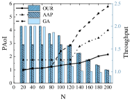
(a) PAoI & Throughout vs. $N$

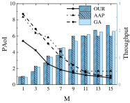
(b) PAoI & Throughout vs. $M$

Figure 2: Impact of methods on various metrics.

In our second set of analyses, we compared our approach, which utilizes strict priority control, with latency-based methods and weight-based (flexible priority control). We explore the latency-based method, focusing on the performance metric of arrival interval. As depicted in Fig.3(a), we found that the latency-based method underperforms in resource-constrained scenarios. The high arrival intervals, indicative of reduced frequency of updates, emerged as a notable limitation in latency-based methods. This shortfall makes them less adept for applications like AR/VR, where there is a critical need for swift information updates [5]. We further compared our approach, which employs hard priority control, with the weight-based method that uses flexible priority control. The results, illustrated in Fig.3(b), showed that our approach effectively reduces the Peak Age of Information (PAoI) for high-priority users. This indicates a more efficient delivery of timely information compared to the weight-based method. The advantage of our approach stems from its server-side priority queuing system, which ensures high-priority tasks are processed more promptly. This experiment underlines the effectiveness of our PAoI-based method in scenarios where speed and accuracy of information processing are paramount.

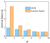
(a) Arrival Internal vs. $\mu$

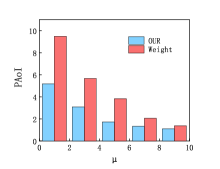
(b) PAoI vs. $\mu$

Figure 3: Performance comparison between different methods.

Our third segment of analysis focuses on the impact of the priorities division and server collaboration on the overall PAoI performance. We conducted a simulation for the multi-priority case, as illustrated in Fig.4(a). Here, $\Delta$ denotes the degree of priority division, with $\Delta=1$ indicating no priority distinction and $\Delta=6$ indicating six priority classes. The simulation results show that the average PAoI of the system is mainly determined by the computing power of the server ($\mu$, task execution time), and the priority division level has little influence on it. Furthermore, we investigate the cases of whether servers are collaborating. Fig.4(b) presents the results for both the server collaboration case and the without-server collaboration case, showing that the PAoI performance of the former outperforms the latter regardless of the number of users. Notably, this feature is more prominent as the number of users $N$ increases. Besides, the PAoI variance in the server collaboration scenario is notably lower, suggesting its stronger system stability.

(a) PAoI vs. $\mu$ in different priority allocation case

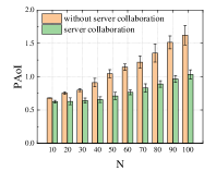
(b) PAoI vs. $N$ in the case of whether servers are collaborating

Figure 4: The performance in various settings.

VI-C Performance of Priority Tasks

Simulation results show that the proposed algorithm can be extended to multi-class priority scenarios. As shown in Fig.5(a), we set three priority classes ($\delta$ lower, higher priority) and then randomly allocated these priority levels to an equal number of users, each of whom had the same quantity of tasks. As the iterations of our algorithm proceed, the average PAoI values of users with various priority levels steadily decrease and eventually tend to stabilize, and the offloading rate gradually increases and eventually tends to be stable. We find that users with higher priority ($\delta=1$) always get higher offloading rates, which results from more channel resource allocations. In addition, high-priority users’ PAoI values are lower since their tasks are scheduled and executed promptly. The above observation implies that high-priority users receive a larger share of channel and computing resources and they are more likely to achieve superior performance.

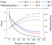
(a) Performance of users with different priorities

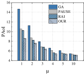
(b) Comparison of high priority users in different algorithms

Figure 5: Performance of Priority Users.

With three types of priorities (high priority, medium priority, low priority), we compare the proposed multi-class priority method (OUR) with other algorithms (GA, PAUSE, RAI). We pay special attention to the promotion effect of our algorithm for high-priority users, as shown in Fig.5(b). The GA algorithm is one that does not consider priorities, the PAUSE algorithm focuses on the discussion of multiple priorities rather than multiple classes of priorities, and the RAI algorithm only considers two classes of priorities. The generality of these methods falls short, and they are unable to provide high-priority users with the lower PAoI that they require. However, it is clear that the proposed strategy our approach is always the best one with the lowest PAoI and can be easily implemented across a range of scenarios.

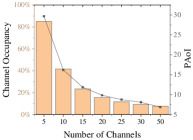
(a) High server processing rates

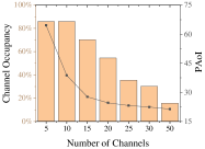
(b) Low server processing rates

Figure 6: PAoI & Channel Occupancy vs. Number of Channels.

VI-D Performance and convergence of Algorithms in Channels

In this subsection, we empirically show the correlation between the algorithm performance and the number of channels, as well as the correlation between the algorithm convergence rate and the channel unreliability.

In order to investigate the potential impact of the number of channels on algorithm performance, we compared the impact of the number of channels on PAoI and average channel occupancy. To this end, we run experiments in two different server processing rates scenarios, as seen in Fig.6(a) and 6(b), respectively. On the one hand, we notice a drop in PAoI as the number climbs, indicating that more tasks may be sent to the server across a more dependable and fast channel as overall channel capacity rises. Particularly, in the scenario of high server processing rates (Fig.6(a)), the server processing efficiency is high, resulting in a lower total PAoI value than in another scenario (Fig.6(b)). On the other hand, as the overall channel capacity increases with the number of channels, the channel occupancy decreases. This ensures that tasks can be transmitted to the server on a more reliable and faster path. However, if the servers’ service efficiency becomes lower than the channel transmission efficiency, there is an upper bound to the channel occupancy. This feature is shown in Fig.6(b) as the number of channels gets low and the reason why it does not reach 100% is discussed in detail in Section III.

The convergence rate of distributed algorithms can be hindered by a lack of reliable communication resources. However, both NFPA-NAC and NFPA-ANAC (as shown in Fig.7(a) and 7(b) respectively) are advantageous for the implementation of powerful edge servers. This is due to their ability to efficiently allocate channel and task-scheduling resources. We show the performance of algorithms NFPA-NAC and NFPA-ANAC in different channel conditions ($p=0.3,0.5,0.7,0.9$) in Fig.7(a) and Fig.7(b) without repeated experiments. We observe that the PAoI values gradually decline and eventually stabilize as the iterations proceed. Moreover, the lower the value of channel condition $p$, the slower the convergence rate. Additionally, it can be observed that PAoI can be more optimal with better channel conditions because users have more options for offloading. We note that in our simulations the algorithm NFPA-NAC cannot successfully iterate in each iteration, while NFPA-ANAC can successfully iterate using the limited information in each iteration.

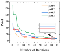
(a) NFPA-NAC

(b) NFPA-ANAC

Figure 7: The influence of the unreliable channel on the PAoI.

To illustrate the differences between the synchronous and asynchronous parallel algorithms, specifically NFPA-NAC and NFPA-ANAC, we can refer to Fig.8. This figure depicts the convergence of these two algorithms under various channel conditions ($p=0.7,0.8,0.9,0.99$). In contrast to Fig.7, we choose a better initial value, more users, and a large number of repeated experiments to help explain the convergence characteristics. Both methods have similar rates of convergence in acceptable channels ($p=0.9,0.99$). However, the convergence rate advantage of algorithm NFPA-ANAC, however, is fairly apparent in the ($p=0.7,0.8$) channel because of the poorer channel quality. This observation verifies our discussion in Section V-A, as it clearly demonstrates that the asynchronous parallel algorithm (NFPA-ANAC) exhibits greater communication efficiency, particularly in unreliable channel conditions.

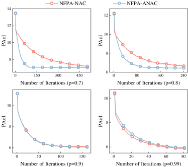
Figure 8: Comparison with different algorithms.

VII Conclusion

In this paper, we proposed a task scheduling method that considered multi-priority users and multi-server collaboration to address the limitations of unreliable channels in current real-time systems and the individual needs of users. We derived the utility function of priority scheduling based on PAoI and designed a set of distributed optimization methods. Specifically, we first considered two simplified problems for the original problem and employed fractional programming as well as ADMM to obtain their solutions. Building upon these solutions and the conclusions drawn therein, we developed an iterative algorithm to solve the original problem. Furthermore, we proposed a distributed asynchronous approach with a sublinear rate of communication defects and discussed the theoretical performance improvement due to the multi-priority mechanism. We implemented the method and conducted extensive simulations to compare it with the existing age-based scheduling strategies. Our results demonstrated the effectiveness and superiority of our method in addressing the requirements of freshness-sensitive users over unreliable channels.

Nan Qiao received the B.Sc. in Computer Science from Central South University, China. Since Sept. 2021, he has been pursuing the Ph.D. degree in Computer Science from Central South University, China. His research interests include wireless communications, distributed optimization, and Internet-of-Things.

Sheng Yue received his B.Sc. in mathematics (2017) and Ph.D. in computer science (2022), from Central South University, China. Currently, he is a postdoc with the Department of Computer Science and Technology, Tsinghua University, China. His research interests include network optimization, distributed learning, and reinforcement learning.

Yongmin Zhang (Senior Member, IEEE) received the PhD degree in control science and engineering in 2015, from Zhejiang University, Hangzhou, China. From 2015 to 2019, he was a postdoctoral research fellow in the Department of Electrical and Computer Engineering at the University of Victoria, BC, Canada. He is currently a Professor in the School of Computer Science and Engineering at the Central South University, Changsha, China. His research interests include IoTs, Smart Grid, and Mobile Computing. He won the best paper award of IEEE PIMRC 2012 and the IEEE Asia-Pacific (AP) outstanding paper award 2018.

Ju Ren Ju Ren [M’16, SM’21] (renju@tsinghua.edu.cn) received the B.Sc. (2009), M.Sc. (2012), Ph.D. (2016) degrees all in computer science, from Central South University, China. Currently, he is an associate professor with the Department of Computer Science and Technology, Tsinghua University, China. His research interests include Internet-of-Things, edge computing, edge intelligence, as well as security and privacy. He currently serves as an associate editor for many journals, including IEEE Transactions on Mobile Computing, IEEE Transactions on Cloud Computing and IEEE Transactions on Vehicular Technology, etc. He also served as the general co-chair for IEEE BigDataSE’20, the TPC co-chair for IEEE BigDataSE’19, the track co-chair for IEEE ICDCS’24, the poster co-chair for IEEE MASS’18, a symposium co-chair for IEEE/CIC ICCC’23&19, I-SPAN’18 and IEEE VTC’17 Fall, etc. He received several best paper awards from IEEE flagship conferences, including IEEE ICC’19 and IEEE HPCC’19, etc., the IEEE TCSC Early Career Researcher Award (2019), and the IEEE ComSoc Asia-Pacific Best Young Researcher Award (2021). He was recognized as a highly cited researcher by Clarivate (2020-2022).

Appendix A

The previous have investigated $\mathbb{E}[T^{p}_{n}]$, $\mathbb{E}[I^{p}_{n}]$ and $\mathbb{E}[Y^{p}_{n}]$ too much, with $\mathbb{E}[Y^{p}_{n}]=1/\mu_{n}$ being the processing time, $\mathbb{E}[T^{p}_{n}]=T^{\mathrm{tr}}_{n,c}$ the maximum transmission time over all possible channels, and $\mathbb{E}[I^{p}_{n}]=1/\sum_{c\in\mathcal{C}}p_{n,c}\eta^{u}_{n,c}\lambda_{n}$ the arrival interval [10]. Also, some studies discuss the waiting time $\mathbb{E}[W]$ in the condition multi-class M/G/1[38] or M/G/1 with priority[43]. However, we focus more on the value of $\mathbb{E}[W]$ in multi-class M/G/1 with priority, which means there are a number of different types of users in a unified priority in the M/G/1 system. According to Little’s Law,

$$\mathbb{E}[L_{i}]=\lambda_{i}\mathbb{E}[W_{i}].$$ (67)

For the highest priority users i.e.$\delta=1$, it holds

$$\mathbb{E}[W_{\delta=1}] =\sum_{i\in\mathcal{N}^{1}}\frac{\mathbb{E}[L_{i}]}{\mu_{i}}+\sum_{i\in\mathcal{N}}\rho_{i}\mathbb{E}[\nu^{2}_{i}]$$

$$=\sum_{i\in\mathcal{N}^{1}}\rho_{i}\mathbb{E}[W_{i}]+\sum_{i\in\mathcal{N}}\rho_{i}\mathbb{E}[\nu^{2}_{i}]$$ (68)

where $\mathbb{E}[W_{\delta=1}]=\mathbb{E}[W_{i}],~{}\forall~{}\delta(i)=1$. Accordingly, we obtain

$$\mathbb{E}[W_{\delta=1}]=\frac{\sum_{i\in\mathcal{N}}\rho_{i}\mathbb{E}[\nu^{2}_{i}]}{1-\sum_{i\in\mathcal{N}^{1}}\rho_{i}}$$ (69)

We separate $\mathbb{E}[W]$ into different components in order to break it down into smaller parts. The first component consists of all high-priority or identically prioritized jobs that are in the queue when the current task arrives. The waiting time for this component is $\mathbb{E}[S^{1}]$. The second component, consisting of all high-priority users who arrived at the same time as the first component was executed, has a waiting time of $\mathbb{E}[S^{2}]$. We continue to split the remaining portions in the same way.

$$\mathbb{E}[W_{i}]=\mathbb{E}[S^{1}_{i}+S^{2}_{i}+S^{3}_{i}+\cdots]=\sum^{\infty}_{k}\mathbb{E}[S^{k}_{i}]$$ (70)

Based on the above discussion, we derive the waiting time for the first part,

$$\mathbb{E}[S^{1}_{i}]=\sum_{p=1}^{\delta(i)}\sum_{j\in\mathcal{N}^{p}}\rho_{j}\mathbb{E}[W_{j}]+\sum_{j\in\mathcal{N}}\rho_{j}\mathbb{E}[\nu^{2}_{j}]$$ (71)

The waiting time for the other part is as follows,

$$E[S^{k+1}_{i}] =\int_{s=0}^{\infty}E[S^{k+1}_{i}\mid S^{k}_{i}=s]f_{k}(s)ds$$

$$=\int_{s=0}^{\infty}\sum_{p=1}^{\delta(i)-1}\sum_{j\in\mathcal{N}^{p}}\rho_{j}sf_{k}(s)ds$$

$$=\left(\sum_{p=1}^{\delta(i)-1}\sum_{j\in\mathcal{N}^{p}}\rho_{j}\right)E[S^{k}_{i}]$$

$$=\left(\sum_{p=1}^{\delta(i)-1}\sum_{j\in\mathcal{N}^{p}}\rho_{j}\right)^{k}E[S^{1}_{i}]$$ (72)

Thus, we derive

$$\mathbb{E}[W_{i}] =\frac{\mathbb{E}[S^{1}_{i}]}{1-\sum_{p=1}^{\delta(i)-1}\sum_{j\in\mathcal{N}^{p}}\rho_{j}}$$

$$=\frac{\sum_{p=1}^{\delta(i)}\sum_{j\in\mathcal{N}^{p}}\rho_{j}\mathbb{E}[W_{j}]+\sum_{j\in\mathcal{N}}\rho_{j}\mathbb{E}[\nu^{2}_{j}]}{1-\sum_{p=1}^{\delta(i)-1}\sum_{j\in\mathcal{N}^{p}}\rho_{j}}$$ (73)

which can be transformed into

$$\mathbb{E}[W_{i}](1-\sum_{p=1}^{\delta(i)-1}\sum_{j\in\mathcal{N}^{p}}\rho_{j})$$

$$=\sum_{p=1}^{\delta(i)}\sum_{j\in\mathcal{N}^{p}}\rho_{j}\mathbb{E}[W_{j}]+\sum_{j\in\mathcal{N}}\rho_{j}\mathbb{E}[\nu^{2}_{j}]$$ (74)

and

$$\mathbb{E}[W_{\delta=\delta(i)}](1-\sum_{p=1}^{\delta(i)}\sum_{j\in\mathcal{N}^{p}}\rho_{j})$$

$$=\sum_{p=1}^{\delta(i)-1}\sum_{j\in\mathcal{N}^{p}}\rho_{j}\mathbb{E}[W_{j}]+\sum_{j\in\mathcal{N}}\rho_{j}\mathbb{E}[\nu^{2}_{j}]$$

$$=\mathbb{E}[W_{\delta=\delta(i)-1}](1-\sum_{p=1}^{\delta(i)-2}\sum_{j\in\mathcal{N}^{p}}\rho_{j})$$ (75)

In other words, it holds,

$$\mathbb{E}[W_{\delta=\delta(i)}](1-\sum_{p=1}^{\delta(i)}\sum_{j\in\mathcal{N}^{p}}\rho_{j})(1-\sum_{p=1}^{\delta(i)-1}\sum_{j\in\mathcal{N}^{p}}\rho_{j})$$ (76)

$$= \mathbb{E}[W_{\delta=\delta(i)-1}](1-\sum_{p=1}^{\delta(i)-1}\sum_{j\in\mathcal{N}^{p}}\rho_{j})(1-\sum_{p=1}^{\delta(i)-2}\sum_{j\in\mathcal{N}^{p}}\rho_{j})$$

Combine with (69), we obtain

$$\mathbb{E}[W_{\delta=\delta(i)}]=\frac{\mathbb{E}[W_{\delta=1}](1-\sum_{j\in\mathcal{N}^{1}}\rho_{j})}{(1-\sum_{p=1}^{\delta(i)}\sum_{j\in\mathcal{N}^{p}}\rho_{j})(1-\sum_{p=1}^{\delta(i)-1}\sum_{j\in\mathcal{N}^{p}}\rho_{j})}$$

$$=\frac{\sum_{i\in\mathcal{N}}\rho_{j}\mathbb{E}[\nu^{2}_{j}]}{(1-\sum_{p=1}^{\delta(i)}\sum_{j\in\mathcal{N}^{p}}\rho_{j})(1-\sum_{p=1}^{\delta(i)-1}\sum_{j\in\mathcal{N}^{p}}\rho_{j})}$$ (77)

which merges the value of $\mathbb{E}[T^{p}_{n}]$, $\mathbb{E}[I^{p}_{n}]$ and $\mathbb{E}[Y^{p}_{n}]$ to complete the proof.

Appendix B A Proof of Lemma 1

First, we should prove that (8) and (11) are not convex sets. Take (8) as an example, if it was a convex set, we should have obtained

$$(1-r)h(\bm{\eta}^{u}_{c_{1}})+rh(\bm{\eta}^{u}_{c_{2}})\mathop{\geq}^{(a)}h((1-r)\bm{\eta}^{u}_{c_{1}}+r\bm{\eta}^{u}_{c_{2}}),$$ (78)

where $h(\bm{\eta}^{u}_{c})=\langle\bm{\lambda},\bm{\eta}^{u}_{c}\rangle+z_{2}\sqrt{\langle\bm{\lambda},\bm{\eta}^{u}_{c}\rangle+z^{2}_{2}/4}+z^{2}_{1}/2-M_{c}^{\mathrm{max}}$, $\bm{\lambda}:=\{\lambda_{n}\}_{n\in\mathcal{N}}$, $\bm{\eta}^{u}_{c}:=\{\eta^{u}_{n,c}|\}_{n\in\mathcal{N}}$, $\forall r\in[0,1]$, $\{c1,c2\in\mathcal{C}\}$, $h(\bm{\eta}^{u}_{c_{1}})\leq 0$ and $h(\bm{\eta}^{u}_{c_{2}})\leq 0$. Moreover, inequality (a) is equivalent to

$$r(r-1)(\sqrt{\langle\bm{\lambda},\bm{\eta}^{u}_{c_{1}}\rangle}+\sqrt{\langle\bm{\lambda},\bm{\eta}^{u}_{c_{2}}\rangle})^{2}\geq 2r(1-r)z^{2}_{2}/4.$$ (79)

However, if $r\neq 0~{}or~{}1$, inequality (79) does not hold since the right term is higher than zero and the left term of the inequality is less than zero. Hence, (8) is a nonconvex set. A comparable procedure in (11) can lead to the same conclusion.

Next, we will demonstrate that (8) and (11) are comparable to (21) and (22) and are convex sets. Again, let’s take the example of (8), which is equivalent to

$$\langle\bm{\lambda},\bm{\eta}^{u}_{c}\rangle+z^{2}_{1}/2+z_{2}\sqrt{\langle\bm{\lambda},\bm{\eta}^{u}_{c}\rangle+z^{2}_{2}/4}\leq M_{c}^{\mathrm{max}},$$

$$(z_{2}/2+\sqrt{\langle\bm{\lambda},\bm{\eta}^{u}_{c}\rangle+z^{2}_{2}/4})^{2}\leq M_{c}^{\mathrm{max}}-z^{2}_{1}/2+z^{2}_{2}/4,$$

$$\langle\bm{\lambda},\bm{\eta}^{u}_{c}\rangle\leq M_{c}^{\mathrm{max}}+\frac{z^{2}_{2}}{2}-\frac{z^{2}_{1}}{2}-z_{2}\sqrt{M_{c}^{\mathrm{max}}+\frac{z^{2}_{2}}{2}-\frac{z^{2}_{1}}{2}},$$ (80)

which means that the constraint (8) is transformed mathematically into (21), which is an affine set and a kind of convex set. (22) can be obtained in a similar way.

Appendix C A Proof of Theorem 1

The objective function that needs to be proven convexity is

$$f_{n}(\hat{t}^{\mathrm{tr}},\bm{\eta}^{u})=F^{T}_{n}(\hat{t}^{\mathrm{tr}}_{n},\bm{\eta}^{u})+F^{I}_{n}(\hat{t}^{\mathrm{tr}}_{n},\bm{\eta}^{u})+F^{W}_{n}(\hat{t}^{\mathrm{tr}}_{n},\bm{\eta}^{u})+F^{Y}_{n}(\hat{t}^{\mathrm{tr}}_{n},\bm{\eta}^{u}),$$

where $F^{I}_{n}(\hat{t}^{\mathrm{tr}}_{n},\bm{\eta}^{u})=F^{I}_{n}(\bm{\eta}^{u})=\frac{1}{\sum_{c\in\mathcal{C}}p_{n,c}\eta^{u}_{n,c}\lambda_{n}}$, $F^{T}_{n}(\hat{t}^{\mathrm{tr}}_{n},\bm{\eta}^{u})=\hat{t}^{\mathrm{tr}}_{n}$, $F^{Y}_{n}(\hat{t}^{\mathrm{tr}}_{n},\bm{\eta}^{u})=\frac{1}{\mu}$, and $F^{W}_{n}(\hat{t}^{\mathrm{tr}}_{n},\bm{\eta}^{u})=F^{W}_{n}(\bm{\eta}^{u})=(\frac{1}{2}\sum_{n^{\prime}=1}^{\mathcal{N}}\sum_{c\in\mathcal{C}}p_{n^{\prime},c}\eta^{u}_{n^{\prime},c}\lambda_{n^{\prime}}\nu)/(1-\sum_{n^{\prime}=1}^{\mathcal{N}}\sum_{c\in\mathcal{C}}p_{n^{\prime},c}\frac{\eta^{u}_{n^{\prime},c}\lambda_{n^{\prime}}}{\mu})$.

1. Due to properties of linear functions, it is obvious that $\nabla^{2}F^{T}_{n}(\hat{t}^{\mathrm{tr}}_{n},\bm{\eta}^{u})\succeq 0$.

2. Due to properties of constant functions, it holds that $\nabla^{2}F^{Y}_{n}(\hat{t}^{\mathrm{tr}}_{n},\bm{\eta}^{u})\succeq 0$.

3. Furthermore, we have $\{n,m,m_{1},m_{2}\in\mathcal{N}|n=m\&n\neq m_{1}\&n\neq m_{2}\}$ , $\{c,d,d_{1},d_{2}\cdots d_{\mathrm{max}}\in\mathcal{C}\}$, $\bm{p}_{n}=\{p_{n,1}\cdots p_{n,C}\}$, and $\bm{p}=\{\bm{p}_{n}|n\in\mathcal{N}\}$. We list some key second-order derivatives.

   $$\frac{\partial^{2}F^{I}_{n}(\bm{\eta}^{u})}{\partial\lambda^{2}_{m,c}} =\frac{2p^{2}_{m,c}}{(\sum_{c\in\mathcal{C}}p_{n,c}\eta^{u}_{n,c}\lambda_{n})^{3}},$$ (81)

   $$\frac{\partial^{2}F^{I}_{n}(\bm{\eta}^{u})}{\partial\lambda_{m,d_{1}}\partial\lambda_{m,d_{2}}} =\frac{2p_{n,d_{1}}p_{n,d_{2}}}{(\sum_{c\in\mathcal{C}}p_{n,c}\eta^{u}_{n,c}\lambda_{n})^{3}},$$ (82)

   $$\frac{\partial^{2}F^{I}_{n}(\bm{\eta}^{u})}{\partial\lambda_{m,c}\partial\lambda_{m_{1},c}} =\frac{\partial^{2}F^{I}_{n}(\bm{\eta}^{u})}{\partial\lambda_{m_{1},c}\partial\lambda_{m_{2},c}}=\frac{\partial^{2}F^{I}_{n}(\bm{\eta}^{u})}{\partial\lambda^{2}_{n_{1},c}}=0.$$ (83)

   Combining Eq.(81), Eq.(82), and Eq.(83), the Hessian matrix of $F^{I}_{n}(\bm{\eta}^{u})$ is described as

   $$\mathbf{H}^{I}_{n}(\bm{\eta}^{u})=\left[\begin{array}[]{c|c}\bm{A}&\bm{B}\\ \hline\cr\bm{C}&\bm{D}\end{array}\right]$$ (86)

   where $\bm{D}=\bm{O}^{(N-1)C}$, $\bm{B}=\bm{C}^{T}=\bm{O}^{C\times(N-1)C}$ and $\bm{A}=\left[\begin{array}[]{ccc}\frac{\partial^{2}F^{I}_{n}(\bm{\eta}^{u})}{\partial\lambda^{2}_{m,d_{1}}}&\cdots&\frac{\partial^{2}F^{I}_{n}(\bm{\eta}^{u})}{\partial\lambda_{m,d_{1}}\partial\lambda_{m,d_{\mathrm{max}}}}\\ \vdots&\ddots&\vdots\\ \frac{\partial^{2}F^{I}_{n}(\bm{\eta}^{u})}{\partial\lambda_{m,d_{\mathrm{max}}}\partial\lambda_{m,d_{1}}}&\cdots&\frac{\partial^{2}F^{I}_{n}(\bm{\eta}^{u})}{\partial\lambda^{2}_{m,d_{\mathrm{max}}}}\end{array}\right]^{C\times C}=\frac{\bm{p}^{T}_{n}\times\bm{p}_{n}}{(\sum_{c\in\mathcal{C}}p_{n,c}\eta^{u}_{n,c}\lambda_{n})^{3}}$ denotes second-order derivative matrix at $m=n$, i.e.$\bm{A}\succeq 0$. The leading Principle Submatrix of $\mathbf{H}^{I}_{n}(\bm{\eta}^{u})$ are all greater than 0, i.e.$\nabla^{2}F^{I}_{n}(\hat{t}^{\mathrm{tr}},\bm{\eta}^{u})\succeq 0$.

4. As for $F^{W}_{n}(\bm{\eta}^{u})$, it holds

   $$\frac{\partial^{2}F^{W}_{n}(\bm{\eta}^{u})}{\partial\lambda_{m_{1},d_{1}}\partial\lambda_{m_{2},d_{2}}}=\bm{p}_{m_{1},d_{1}}\bm{p}_{m_{2},d_{2}}\frac{\nu/\mu}{(1-\sum_{m=1}^{\mathcal{N}}\sum_{c\in\mathcal{C}}p_{m,c}\frac{\lambda_{m,c}}{\mu})^{3}}$$ (87)

   The hessian matrix is described as

   $$\nabla^{2}F^{W}_{n}(\bm{\eta}^{u})=\bm{p}^{T}\times\bm{p}\frac{\nu/\mu}{(1-\sum_{m=1}^{\mathcal{N}}\sum_{c\in\mathcal{C}}p_{m,c}\frac{\lambda_{m,c}}{\mu})^{3}}$$ (88)

   Thus, we derive $\nabla^{2}F^{W}_{n}(\hat{t}^{\mathrm{tr}},\bm{\eta}^{u})\succeq 0$.

Above all, $\nabla^{2}f_{n}(\hat{t}^{\mathrm{tr}},\bm{\eta}^{u})\succeq 0$. The proof is completed.

Appendix D Details of Optimal Solution to P1

In this section, we delve into the intricacies of the optimal solution for problem P1 in detail. We elucidate the Algorithm AC, tailored for solving P1, and expound on its comprehensive procedure in Appendix D-A. The convergence properties and proofs pertaining to Algorithm AC are methodically analyzed in Appendix D-B. Furthermore, we expand upon Algorithm AC in Appendix D-C by architecting its asynchronous variant, thereby enhancing its communication efficacy in the context of unreliable channels. This enhancement paves the way for deeming the algorithm as adept in managing communication challenges within such environments.

D-A Algorithm AC for the solution to P1

According to Problem P1-3, the augmented Lagrangian for Problem P1-3 can be expressed as:

$$L_{\rho}(\{\bm{x}_{n}\},\bm{x}_{o},\{\bm{\sigma}_{n}\}) =\sum_{n\in\mathcal{N}}(g_{n}(\bm{x}_{n})+\langle\bm{\sigma}_{n},\bm{x}_{n}-\bm{x}_{o}\rangle$$

$$+(\rho/2)\|\bm{x}_{n}-\bm{x}_{o}\|^{2}_{2},$$ (89)

where $\bm{\sigma}_{n}:=\{\sigma^{n}_{m,c}|c\in\mathcal{C},m\in\mathcal{N}\}$ denotes the Lagrangian multipliers P1-3 and $\rho$ is a positive penalty parameter. Based on the analysis of Theorem 1 and Section IV-A2, the ADMM-Consensus based offloading algorithm is summarized as Algorithm 5. The procedure is detailed subsequently:

User side

In iteration $t$ of the loop, given $\bm{x}_{n}$, the primal and dual variables are updated according to Eq. (D-A) and Eq. (91), respectively. Then, each user sends the $\bm{x}^{t+1}_{n}$ and $\bm{\sigma}^{t+1}_{n}$ to the local server.

$$\bm{x}^{t+1}_{n} =\arg\min_{\bm{x}_{n}}(g_{n}(\bm{x}_{n})+\langle\bm{\sigma}^{t},\bm{x}_{n}-\bm{x}_{o}\rangle$$

$$+(\rho/2)\|\bm{x}_{n}-\bm{x}^{t}_{o}\|^{2}_{2}),$$ (90)

$$\bm{\sigma}^{t+1}_{n} =\bm{\sigma}^{t}_{n}+\rho(\bm{x}^{t+1}_{n}-\bm{x}^{t}_{o}).$$ (91)

Server side

The server aggregates all the iterations it receives, updates the value of $\bm{x}^{t+1}_{o}$ according to Eq. (92), and circulates the updated information back to the users.

$$\bm{x}^{t+1}_{o} =\frac{1}{N}\sum_{n\in\mathcal{N}}(\bm{x}^{t+1}_{n}+(\frac{1}{\rho}\bm{\sigma}^{t+1}_{n})).$$ (92)

Termination criteria

The iterative process is terminated when primal residual $\|\bm{x}^{t+1}_{n}-\bm{x}^{t+1}_{o}\|^{2}_{2}$ exceeds a predefined threshold $\epsilon^{\mathit{pr}}$, or when dual residual $\rho\|\bm{x}^{t+1}_{o}-\bm{x}^{t}_{o}\|^{2}_{2}$ surpasses the threshold $\epsilon^{\mathrm{dl}}$.

1 for $n=1$ to $N$ do

       Input: $\epsilon^{\mathit{pr}}$, $\epsilon^{\mathrm{dl}}$, $\theta$, $\bm{x}_{n}$, $t$

2       while $\|\bm{x}^{t+1}_{n}-\bm{x}^{t+1}_{o}\|^{2}_{2}>\epsilon^{\mathit{pr}}$ or $\rho\|(\bm{x}^{t+1}_{o})-\bm{x}^{t}_{o})\|^{2}_{2}>\epsilon^{\mathrm{dl}}$ do

3             Calculate $\bm{x}^{t+1}_{n}$, simultaneously according to (D-A)

4             Calculate $\sigma^{t+1}_{n}$, according to (91)

5             Calculate $\bm{x}^{t+1}_{o}$, according to (92)

6             Update $t=t+1$

7            

8       end while

9      Set $\bm{x}^{*}_{n}=\bm{x}^{t+1}_{n}$

       Output: $\bm{x}^{*}_{n}$

10      

11 end for

Algorithm 5 ADMM-Consensus (AC)

D-B The performance analysis of Algorithm AC

In this subsection, we further analyze the convergence and computational cost of the Algorithm AC. According to Theorem 1, the objective function of Problem P1-3 is defined as a closed, proper, and convex function. Its associated domain is also a well-defined closed, non-empty convex set. Moreover, the Lagrangian $L_{n}\left(\left\{\bm{x}_{n}^{t+1}\right\},\bm{x}_{o}^{t+1};y^{t+1}\right)$ is endowed with a saddle point. Consequently, based on [56], the iteration is demonstrated to satisfy three types of convergence: dual, consensus, and objective function. These convergences are explicated as follows:

• Dual variable convergence. We have $\sigma^{t}_{n}\rightarrow\sigma^{*}_{n}$ as $t\rightarrow\infty$, where $\sigma^{*}_{n}$ is a dual optimal vector.

• Consensus convergence. The consensus constraint is satisfied eventually $\lim_{t\rightarrow\infty}\left\|\bm{x}_{n}^{t+1}-\bm{x}_{o}^{t+1}\right\|=0,\forall n$.

• Objective function convergence. The objective function ultimately stabilizes at the optimal value:

  $$\sum_{n\in\mathcal{N}}g_{n}(\bm{x}^{t})\rightarrow\sum_{n\in\mathcal{N}}g_{n}(\bm{x}^{*}_{n}),~{}t\rightarrow\infty$$ (93)

Within each iteration of the Algorithm 5, Eq. (D-A), Eq. (91), and Eq. (92) are updated in a sequential manner to get $\bm{x}^{t}$. Accordingly, each individual subproblem can be efficiently tackled using prevalent optimization techniques such as gradient descent or interior point methods with low computational costs.

D-C Detail of Asynchronous Solution to P1-3

In the preceding subsections, we introduced a suite of synchronous parallel algorithms. However, the robustness and performance of these algorithms are significantly susceptible to disruptions caused by communication errors and the inherent unreliability of wireless communication networks [13]. This emphasizes the imperative to transition towards an alternative that is more resilient and economizes on communication costs. Consequently, we introduce the distributed asynchronous ADMM algorithm tailored for consensus optimization of the global variable.

To guarantee the progression of an asynchronous algorithm, it is essential to establish a cap on the requisite number of communications per communicative entity. To adhere to the iteration delay bound necessary for effective communication, denoted as $\Gamma_{n}$, the inequality $(1-p^{\text{max}}_{n})^{\Gamma_{n}}<\epsilon^{a}$ holds, where $\epsilon^{a}$ represents the maximal allowable delay for asynchronous iteration exchanges. By taking the logarithm of both sides, we arrive at the inequality $\Gamma_{n}\geq\frac{\ln(\epsilon^{a})}{\ln(1-p^{\text{max}}_{n})}$. Consequently, we assume the following:

Assumption 2.

The communication rounds required to conclude a successful iteration are bounded above by

$$\Gamma_{n}=\left\lceil\frac{\ln(\epsilon^{a})}{\ln(1-p^{\text{max}}_{n})}\right\rceil,$$ (94)

where $\lceil x\rceil$ denotes the smallest integer greater than or equal to $x$.

This assumption is a conventional one in studies of asynchronous ADMM, as referenced in works such as [58, 59]. In the worst case, this condition is pivotal to ensuring that each participant completes at least one iteration within $\Gamma_{n}$ cycles.

Updating $\bm{x}_{n}$ and $\bm{\sigma}_{n}$ in Users

We first update the variables $\bm{x}_{n}$ and $\bm{\sigma}_{n}$ as follows:

$$\bm{x}^{t+1}_{n} =\arg\min_{\bm{x}_{n}}(g_{n}(\bm{x}_{n})+\langle\bm{\sigma}^{t},\bm{x}_{n}-\bm{x}_{o}\rangle$$

$$+(\rho/2)\|\bm{x}_{n}-\bm{x}^{t}_{o}\|^{2}_{2}),$$ (95)

$$\bm{\sigma}^{t+1}_{n} =\bm{\sigma}^{t}_{n}+\rho(\bm{x}^{t+1}_{n}-\bm{x}^{t+1}_{o}),$$ (96)

where the most recent consensus value $\bm{x}_{o}$ is received from the server. Furthermore, the termination criteria are the same as in Algorithm 5. Accordingly, the user-side procedure is delineated in Algorithm 6:

Input: $\bm{\sigma}_{n}^{0},t$ for all users $n$

Output: Optimized parameter $x_{o}^{*}$

1 while $\|\bm{x}^{t+1}_{n}-\bm{x}^{t+1}_{o}\|^{2}_{2}>\epsilon^{\mathit{pr}}$ or $\rho\|(\bm{x}^{t+1}_{o})-\bm{x}^{t}_{o})\|^{2}_{2}>\epsilon^{\mathrm{dl}}$ do

2       Update $\bm{x}_{n}^{t+1}$ using Eq. (D-C)

3       Update $\bm{\sigma}^{t+1}_{n}$ using Eq. (96)

4       Send $\bm{\sigma}_{n}^{t}$ and $\bm{x}_{n}^{t+1}$ to the Server

5       Wait for $\bm{x}^{n}_{o}$ from the Server

6       Update $\bm{\sigma}_{n}^{t+1}$ using (8)

7       $t\leftarrow t+1$

8      

9 end while

Algorithm 6 Asynchronous ADMM-Consensus in Users (AACU)

Updating $\bm{x}_{o}$ in Server

As shown in Algorithm 7, the server continuously accumulates updates from users until it has gathered a minimum of $N_{\mathrm{min}}$ updates or until the maximum delay surpasses a threshold, designated as $\Gamma=\max\{\Gamma_{1}\cdots\Gamma_{N}\}$. In this context, the set of users who have submitted updates in phase $t$ is denoted as $\Phi^{t}$. For each user $n$ within this group, their corresponding $\bm{x}_{n}$ and $\bm{\sigma}_{n}$ values are updated. Conversely, for those not in $\Phi^{t}$, their values remain unchanged. Upon completion of this process, the server proceeds to update the value of $\bm{x}_{o}$ in accordance with Eq. (97) and subsequently broadcasts this revised value.

$$\bm{x}^{t+1}_{o} =\frac{1}{N}\sum_{n\in\mathcal{N}}(\bm{x}^{t+1}_{n}+(\frac{1}{\rho}\bm{\sigma}^{t}_{n})),$$ (97)

Input: $t,\bm{x}_{n},\bm{\sigma}_{n}$ for $i=1,2,\ldots,N$

Output: Optimized parameter $\bm{x}_{o}^{*}$

1 Initialize

2 while $\|\bm{x}^{t+1}_{n}-\bm{x}^{t+1}_{o}\|^{2}_{2}>\epsilon^{\mathit{pr}}$ or $\rho\|(\bm{x}^{t+1}_{o})-\bm{x}^{t}_{o})\|^{2}_{2}>\epsilon^{\mathrm{dl}}$ do

3       $\tau_{n}\leftarrow 0$ for $n=1,2,\ldots,N$

4       while less than $N_{\mathrm{min}}$ updates received or $\max(\tau_{1},\tau_{2},\ldots,\tau_{N})>\Gamma$ do

5             Wait for updates

6            

7       end while

8      foreach user $n\in\Phi^{t}$ do

9             $\tau_{n}\leftarrow 1$

10             $\bm{x}_{n}\leftarrow$ newly received $\bm{x}_{n}$ from user $n$

11             $\bm{\sigma}_{n}\leftarrow$ newly received $\sigma_{n}$ from user $n$

12            

13       end foreach

14      foreach user $n\notin\Phi^{t}$ do

15             $\tau_{n}\leftarrow\tau_{n}+1$

16            

17       end foreach

18      Update $\bm{x}_{o}^{t+1}$ by Eq. (97)

19       Broadcast $\bm{x}_{o}^{t+1}$ to all the users in $\Phi^{t}$

20       $k\leftarrow t+1$

21      

22 end while

Algorithm 7 Asynchronous ADMM-Consensus by Server (AACS)

Theorem 5.

Let $(x^{*},\bm{x}_{o}^{*})$ represent the optimal primal solution of problem P1-3, and $\{\bm{\sigma}_{n}^{*}\}_{n=1}^{N}$ the corresponding optimal dual solution. Then,

$$\mathbb{E}\left[\sum_{n=1}^{N}g_{n}(\bm{x}_{n})-g_{n}(\bm{x}^{*})+\langle\bm{\sigma}_{n}^{*},\bm{x}_{n}-\bm{x}_{o}^{*}\rangle\right]$$

$$\leq \frac{N\Gamma}{2TN_{\mathrm{min}}}\left\{\sum_{n=1}^{N}\rho\|\bm{x}_{o}^{0}-\bm{x}_{o}^{*}\|^{2}+\frac{1}{\rho}\|\bm{\sigma}_{n}^{0}-\bm{\sigma}_{n}^{*}\|^{2}\right\},$$ (98)

where $\bm{x}_{o}^{0}$ and $\bm{\sigma}_{n}^{0}$ denote the initial values of $\bm{x}_{o}$ and $\bm{\sigma}_{n}$, respectively, for user $n$.

Proof.

The result of Theorem 5 can be obtained via the proof of combining [63, Theorem 4.2] and [63, Corollary 4.3]. ∎

Consequently, the theorem 5 implies that the combination of Algorithms 6 and 7 can sublinearly converge. Specifically, the asynchronous algorithm convergence rate is $O(\frac{N\Gamma}{TN_{\mathrm{min}}})$.

Appendix E A Proof of Proposition 1

A brief idea of the proof is given as follows. According to nonlinear fractional programming [57], $\theta^{*}_{n}$ is achieved if and only if

$$\mathop{\min}_{\bm{x}_{n}}f^{p,u}_{n}(\bm{x}_{n})-\theta^{*}_{n}f^{p,l}_{n}(\bm{x}_{n})$$

$$=f^{p,u}_{n}(\bm{x}_{n}^{*})-\theta^{*}_{n}f^{p,l}_{n}(\bm{x}_{n}^{*})=0.$$ (99)

which outlines the necessary and sufficient criteria in order to reach $\theta^{*}_{n}$. In light of this, $\{\bm{x}_{n}\}$ can be acquired by resolving the following transformation problem.

Appendix F A Proof of Proposition 2

Here is a concise proof followed by a comprehensive one.

F-A A Concise Proof

1. Given the complexity of the proof, we will only provide a brief overview of the main idea here. We begin by computing the Hessian matrix of the entire function. Due to differing priority attributes ($\delta(n_{1})>\delta(n_{2})$, $\delta(n_{1})=\delta(n_{2})$, n1=n2,$\delta(n_{1})<\delta(n_{2})$), we need to examine the second derivative of the function in at least 16 cases.

2. Through analyzing the properties of the Hessian matrix, we observe that the function is Lipschitz smooth or gradient Lipschitz continuous as long as the values in the Hessian matrix are finite.

3. We can also obtain the value of $\ell_{n}$in $\ell_{n}I\succeq\nabla^{2}F$ based on the characteristics of the Hessian matrix.

F-B A Comprehensive Proof

For computational convenience, we present some functions, where $\Phi_{\delta(n)}(\bm{x})=1-\sum_{\delta=1}^{\delta(n)}\sum_{n^{\prime}=1}^{\mathcal{N}^{\delta}}\sum_{c\in\mathcal{C}}p_{n^{\prime},c}\frac{\eta^{u}_{n^{\prime},c}\lambda_{n^{\prime}}}{\mu_{n^{\prime}}}$, $\Phi_{0}(\bm{x})=1$, $\Upsilon(\bm{x})=\frac{1}{2}\sum_{\delta=1}^{\Delta}\sum_{n^{\prime}=1}^{\mathcal{N}^{\delta}}\sum_{c\in\mathcal{C}}p_{n^{\prime},c}\eta^{u}_{n^{\prime},c}\lambda_{n^{\prime}}\nu_{n^{\prime}}$, and $\Psi_{n}(\bm{x})=\sum_{c\in\mathcal{C}}p_{n,c}\eta^{u}_{n,c}\lambda_{n}$. We also give some useful parameters in advance, where $\{n_{1},n_{2}\in\mathcal{N}\}$, $\{c_{1},c_{2}\in\mathcal{C}\}$, $\kappa_{1}=\frac{p_{n_{1},c_{1}}}{\mu_{n_{1}}}>0$, $\kappa^{1}_{\mathrm{max}}=\frac{1}{\mu_{\mathrm{min}}}>0$, and $p_{n,c}\in[0,1]$. Additionally, since $\nabla_{\{t^{\mathrm{tr}}\in\bm{x}\}}g^{p}_{n}(\bm{x})=0$, we just ignore it. Due to $\nabla^{2}_{\eta_{n_{1},c_{1}}\eta_{n_{2},c_{2}}}g^{p}_{n}(\bm{x})=\lambda_{n_{1}}\lambda_{n_{2}}\nabla^{2}_{\lambda_{n_{1},c_{1}}\lambda_{n_{2},c_{2}}}g^{p}_{n}(\bm{x})$, we have

F-B1 Hessian Matrix

We first analyze the function $f^{p,u}_{n}(\bm{x})$,

$$f^{p,u}_{n}(\bm{x}) =\Phi_{\delta(n)}(\bm{x})\Phi_{\delta(n)-1}(\bm{x})+\Upsilon(\bm{x})\Psi_{n}(\bm{x}).$$ (100)

Case I) If $\delta(n_{1})<\delta(n)$, we obtain first-order derivative.

$$\frac{\partial f^{p,u}_{n}(\bm{x})}{\partial\lambda_{n_{1},c_{1}}} =-\frac{p_{n_{1},c_{1}}}{\mu_{n_{1}}}(\Phi_{\delta(n)}(\bm{x})+\Phi_{\delta(n)-1}(\bm{x}))$$

$$+\frac{1}{2}p_{n_{1},c_{1}}\nu_{n_{1}}\Psi_{n}(\bm{x})$$ (101)

We obtain some second-order derivatives.

$$\frac{\partial^{2}f^{p,u}_{n}(\bm{x})}{\partial\lambda_{n_{1},c_{1}}\partial\lambda_{n_{2},c_{2}}}\\ =\left\{\begin{array}[]{ll}2\frac{p_{n_{1},c_{1}}p_{n_{2},c_{2}}}{\mu_{n_{1}}\mu_{n_{2}}},\quad\delta(n_{2})<\delta(n)\\ \frac{p_{n_{1},c_{1}}p_{n_{2},c_{2}}}{\mu_{n_{1}}\mu_{n_{2}}}+\frac{1}{2}p_{n_{1},c_{1}}p_{n_{2},c_{2}}\nu_{n_{1}},\quad n_{2}=n\\ \frac{p_{n_{1},c_{1}}p_{n_{2},c_{2}}}{\mu_{n_{1}}\mu_{n_{2}}},\quad\delta(n_{2})=\delta(n),\quad n_{2}\neq n\\ 0,\quad\delta(n_{2})>\delta(n)\\ \end{array}\right..$$ (102)

Case II) If $\delta(n_{1})=\delta(n)~{}\&~{}n_{1}=n$, we obtain first-order derivative.

$$\frac{\partial f^{p,u}_{n}(\bm{x})}{\partial\lambda_{n_{1},c_{1}}} =-\frac{p_{n_{1},c_{1}}}{\mu_{n_{1}}}\Phi_{\delta(n)-1}(\bm{x})+p_{n_{1},c_{1}}\Upsilon(\bm{x})$$

$$+\frac{1}{2}p_{n_{1},c_{1}}\nu_{n_{1}}\Psi_{n}(\bm{x})$$ (103)

We obtain some second-order derivatives.

$$\frac{\partial^{2}f^{p,u}_{n}(\bm{x})}{\partial\lambda_{n_{1},c_{1}}\partial\lambda_{n_{2},c_{2}}}=\left\{\begin{array}[]{ll}&\frac{p_{n_{1},c_{1}}p_{n_{2},c_{2}}}{\mu_{n_{1}}\mu_{n_{2}}}+\frac{1}{2}p_{n_{1},c_{1}}p_{n_{2},c_{2}}\nu_{n_{2}},\\ &\quad\delta(n_{2})<\delta(n)\\ &\frac{1}{2}p_{n_{1},c_{1}}p_{n_{2},c_{2}}\nu_{n_{1}}+\frac{1}{2}p_{n_{1},c_{1}}p_{n_{2},c_{2}}\nu_{n_{2}},\\ &\quad n_{2}=n\\ &\frac{1}{2}p_{n_{1},c_{1}}p_{n_{2},c_{2}}\nu_{n_{2}},\quad\delta(n_{2})=\delta(n),\\ &\quad n_{2}\neq n\\ &\frac{1}{2}p_{n_{1},c_{1}}p_{n_{2},c_{2}}\nu_{n_{2}},\quad\delta(n_{2})>\delta(n)\\ \end{array}\right..$$

Case III) If $\delta(n_{1})=\delta(n)~{}\&~{}n_{1}\neq n$, we obtain first-order derivative.

$$\frac{\partial f^{p,u}_{n}(\bm{x})}{\partial\lambda_{n_{1},c_{1}}}=-\frac{p_{n_{1},c_{1}}}{\mu_{n_{1}}}\Phi_{\delta(n)-1}(\bm{x})+\frac{1}{2}p_{n_{1},c_{1}}\nu_{n_{1}}\Psi_{n}(\bm{x})$$ (104)

We obtain some second-order derivatives.

$$\frac{\partial^{2}f^{p,u}_{n}(\bm{x})}{\partial\lambda_{n_{1},c_{1}}\partial\lambda_{n_{2},c_{2}}}=\left\{\begin{array}[]{ll}&\frac{p_{n_{1},c_{1}}p_{n_{2},c_{2}}}{\mu_{n_{1}}\mu_{n_{2}}},\quad\delta(n_{2})<\delta(n)\\ &\frac{1}{2}p_{n_{1},c_{1}}p_{n_{2},c_{2}}\nu_{n_{1}},\quad n_{2}=n\\ &0,\quad\delta(n_{2})=\delta(n),\quad n_{2}\neq n\\ &0,\quad\delta(n_{2})>\delta(n)\\ \end{array}\right..$$ (105)

Case IV) If $\delta(n_{1})>\delta(n)$, we obtain first-order derivative.

$$\frac{\partial f^{p,u}_{n}(\bm{x})}{\partial\lambda_{n_{1},c_{1}}}=\frac{1}{2}p_{n_{1},c_{1}}\nu_{n_{1}}\Psi_{n}(\bm{x})$$ (106)

We obtain some second-order derivatives.

$$\frac{\partial^{2}f^{p,u}_{n}(\bm{x})}{\partial\lambda_{n_{1},c_{1}}\partial\lambda_{n_{2},c_{2}}}=\left\{\begin{array}[]{ll}&0,\quad\delta(n_{2})<\delta(n)\\ &\frac{1}{2}p_{n_{1},c_{1}}p_{n_{2},c_{2}}\nu_{n_{1}},\quad n_{2}=n\\ &0,\quad\delta(n_{2})=\delta(n),\quad n_{2}\neq n\\ &0,\quad\delta(n_{2})>\delta(n)\\ \end{array}\right..$$ (107)

As for $f^{p,l}_{n}(\bm{x})$, we have some different cases, as follows.

$$f^{p,l}_{n}(\bm{x}) =\Psi_{n}(\bm{x})\Phi_{\delta(n)}(\bm{x})\Phi_{\delta(n)-1}(\bm{x}).$$ (108)

Case I) If $\delta(n_{1})<\delta(n)$, we obtain first-order derivative.

$$\frac{\partial f^{p,l}_{n}(\bm{x})}{\partial\lambda_{n_{1},c_{1}}}=-\frac{p_{n_{1},c_{1}}}{\mu_{n_{1}}}(\Phi_{\delta(n)}(\bm{x})+\Phi_{\delta(n)-1}(\bm{x}))\Psi_{n}(\bm{x})$$ (109)

We obtain some second-order derivatives.

$$\noindent\frac{\partial^{2}f^{p,l}_{n}(\bm{x})}{\partial\lambda_{n_{1},c_{1}}\partial\lambda_{n_{2},c_{2}}}$$

$$=\left\{\begin{array}[]{ll}&2\frac{p_{n_{1},c_{1}}p_{n_{2},c_{2}}}{\mu_{n_{1}}\mu_{n_{2}}}\Psi_{n}(\bm{x}),\quad\delta(n_{2})<\delta(n)\\ &\frac{p_{n_{1},c_{1}}p_{n_{2},c_{2}}}{\mu_{n_{1}}\mu_{n_{2}}}(\Psi_{n}(\bm{x})-\frac{\nu_{n_{2}}}{2\mu_{n_{2}}}\Phi_{\delta(n)}(\bm{x})-\frac{\nu_{n_{2}}}{2\mu_{n_{2}}}\Phi_{\delta(n)-1}(\bm{x})),\\ &~{}~{}~{}\quad n_{2}=n\\ &\frac{p_{n_{1},c_{1}}p_{n_{2},c_{2}}}{\mu_{n_{1}}\mu_{n_{2}}}\Psi_{n}(\bm{x}),\quad\delta(n_{2})=\delta(n),\quad n_{2}\neq n\\ &0,\quad\delta(n_{2})>\delta(n)\\ \end{array}\right..$$ (110)

Case II) If $\delta(n_{1})=\delta(n)~{}\&~{}n_{1}=n$, we obtain first-order derivative.

$$\frac{\partial f^{p,l}_{n}(\bm{x})}{\partial\lambda_{n_{1},c_{1}}} =p_{n_{1},c_{1}}\Phi_{\delta(n)}(\bm{x})\Phi_{\delta(n)-1}(\bm{x})$$

$$-\frac{p_{n_{1},c_{1}}}{\mu_{n_{1}}}\Psi_{n}(\bm{x})\Phi_{\delta(n)-1}(\bm{x})$$ (111)

We obtain some second-order derivatives.

$$\frac{\partial^{2}f^{p,l}_{n}(\bm{x})}{\partial\lambda_{n_{1},c_{1}}\partial\lambda_{n_{2},c_{2}}}$$

$$=\left\{\begin{array}[]{ll}&\frac{p_{n_{1},c_{1}}p_{n_{2},c_{2}}}{\mu_{n_{1}}\mu_{n_{2}}}(\Psi_{n}(\bm{x})-\frac{\nu_{n_{2}}}{2\mu_{n_{2}}}\Phi_{\delta(n)}(\bm{x})-\frac{\nu_{n_{2}}}{2\mu_{n_{2}}}\Phi_{\delta(n)-1}(\bm{x})),\\ &\quad\delta(n_{2})<\delta(n)\\ &-\frac{p_{n_{1},c_{1}}p_{n_{2},c_{2}}}{\mu_{n_{1}}\mu_{n_{2}}}(\frac{\nu_{n_{1}}}{2\mu_{n_{1}}}+\frac{\nu_{n_{2}}}{2\mu_{n_{2}}})\Phi_{\delta(n)-1}(\bm{x}),\quad n_{2}=n\\ &-\frac{p_{n_{1},c_{1}}p_{n_{2},c_{2}}}{\mu_{n_{1}}\mu_{n_{2}}}\frac{\nu_{n_{2}}}{2\mu_{n_{2}}}\Phi_{\delta(n)-1}(\bm{x}),\quad\delta(n_{2})=\delta(n),\quad n_{2}\neq n\\ &0,\quad\delta(n_{2})>\delta(n)\\ \end{array}\right..$$ (112)

Case III) If $\delta(n_{1})=\delta(n)~{}\&~{}n_{1}\neq n$, we obtain first-order derivative.

$$\frac{\partial f^{p,l}_{n}(\bm{x})}{\partial\lambda_{n_{1},c_{1}}}=-\frac{p_{n_{1},c_{1}}}{\mu_{n_{1}}}\Psi_{n}(\bm{x})\Phi_{\delta(n)-1}(\bm{x})$$ (113)

We obtain some second-order derivatives.

$$\frac{\partial^{2}f^{p,l}_{n}(\bm{x})}{\partial\lambda_{n_{1},c_{1}}\partial\lambda_{n_{2},c_{2}}}=\left\{\begin{array}[]{ll}&\frac{p_{n_{1},c_{1}}p_{n_{2},c_{2}}}{\mu_{n_{1}}\mu_{n_{2}}}\Psi_{n}(\bm{x}),\quad\delta(n_{2})<\delta(n)\\ &-\frac{p_{n_{1},c_{1}}p_{n_{2},c_{2}}}{\mu_{n_{1}}\mu_{n_{2}}}\frac{\nu_{n_{2}}}{2\mu_{n_{2}}}\Phi_{\delta(n)-1}(\bm{x}),\quad n_{2}=n\\ &0,\quad n_{2}\neq n\\ &0,\quad\delta(n_{2})>\delta(n)\\ \end{array}\right..$$ (114)

Case IV) If $\delta(n_{1})>\delta(n)$, we obtain first and second-order derivative.

$$\frac{\partial f^{p,l}_{n}(\bm{x})}{\partial\lambda_{n_{1},c_{1}}}=0 \frac{\partial^{2}f^{p,l}_{n}(\bm{x})}{\partial\lambda_{n_{1},c_{1}}\partial\lambda_{n_{2},c_{2}}}=0.$$ (115)

Above all, we have the first-order derivative and the second-order derivative information of $g^{p}_{n}(\bm{x})=f^{p,u}_{n}(\bm{x})-\theta^{*}_{n}f^{p,l}_{n}(\bm{x})$.

F-B2 The Relationship between Hessian Matrix and Lipschitz Smooth

Obviously, for any $n$, $g^{p}_{n}(\bm{x})$ is a smooth function.

On the other hand, the twice differentiable function $g^{p}_{n}(\bm{x})$ has a Lipschitz continuous gradient with modulus $\ell_{n}$ if and only if its Hessian satisfies $\ell_{n}I\succeq\nabla^{2}g^{p}_{n}(\bm{x})$. We have $\ell_{n}$ is equal to the maximum eigenvalue of $\nabla^{2}g^{p}_{n}(\bm{x})$,[64].

In order to obtain the maximum eigenvalue, we ought to get the maximum value of the sum of the absolute values of the elements of the column of the matrix $\nabla^{2}g^{p}_{n}(\bm{x})$, which is because that if $\xi$ is the eigenvector of matrix $\mathcal{A}$ with respect to eigenvalue $\omega$.

According to the basic property, we have $\sum_{j=1}^{n}A_{ij}\xi_{j}=\omega\xi_{i}$, i.e.$\sum_{j=1}^{n}\left|A_{ij}\right|\left|\xi_{j}\right|\geq|\omega|\left|\xi_{i}\right|$.

Summing over both sides, it is

$$\sum_{i=1}^{n}\sum_{j=1}^{n}\left|A_{ij}\right|\left|\xi_{j}\right|\geq\sum_{i=1}^{n}|\omega|\left|\xi_{i}\right|$$ (116)

Let $M=\max_{1\leq j\leq n}\sum_{i=1}^{n}\left|A_{ij}\right|$, we have

$$M\sum_{j=1}^{n}\left|\xi_{j}\right|\geq\sum_{j=1}^{n}\left|\xi_{j}\right|\sum_{i=1}^{n}\left|A_{ij}\right|\geq\sum_{i=1}^{n}|\omega|\left|\xi_{i}\right|\geq|\omega|\sum_{i=1}^{n}\left|\xi_{i}\right|$$ (117)

Since $\xi$ is not a zero vector, we obtain

$$|\omega|\leq\max_{1\leq j\leq n}\sum_{i=1}^{n}\left|A_{ij}\right|$$ (118)

F-B3 Solve for the value of $\ell_{n}$

Upper bound on the sum of the absolute values of the elements in the columns of the matrix $\nabla^{2}_{\bm{\eta}^{u}}g^{p}_{n}(\bm{x})$ is expressed as $\varphi(\bm{x})\lambda^{2}_{max}$ with $\lambda_{max}=\mathop{\max}_{n}{\lambda_{n}}$:

$$\varphi(\bm{x}) \leq\mathop{\max}\Big{\{}\inf|\varphi_{1}(\bm{x})|,\inf|\varphi_{2}(\bm{x})|,\inf|\varphi_{3}(\bm{x})|,\inf|\varphi_{4}(\bm{x})|\Big{\}}$$

$$\mathop{\leq}^{(a)}\mathop{\max}\Big{\{}\inf|\varphi_{1}(\bm{x})|,\inf|\varphi_{2}(\bm{x})|,\inf|\varphi_{3}(\bm{x})|\Big{\}}$$

$$\mathop{\leq}^{(b)}\mathop{\max}\Big{\{}\inf|\varphi_{1}(\bm{x})|,\inf|\varphi_{3}(\bm{x})|\Big{\}}$$

$$\mathop{\leq}^{(c)}\mathop{\max}\Big{\{}\inf|\varphi_{3}(\bm{x})|\Big{\}}$$

$$\mathop{\leq}^{(d)}\frac{1}{\mu^{2}_{\mathrm{min}}}\Big{(}\sum_{n_{1}\in\mathcal{N}}|\frac{\nu_{n}}{2\mu_{n}\mu_{n_{1}}}|+\sum_{n_{1}\in\{<\delta(n)\}\bigcup\{n\}}|1+\theta^{*}_{n}\frac{\nu_{n}}{2\mu_{n}}|$$

$$~{}~{}~{}~{}+\sum_{n_{1}\in\{\leq\delta(n)\}}|\theta^{*}_{n}\frac{\nu_{n}}{2\mu_{n}}|\Big{)},$$ (119)

where $\varphi_{1}(\bm{x})$, $\varphi_{2}(\bm{x})$, $\varphi_{3}(\bm{x})$, and $\varphi_{4}(\bm{x})$ are

Case I) If $\delta(n_{2})<\delta(n)$, we have

$$\varphi_{1}(\bm{x}) =\overbrace{\sum_{n_{1}\in\{<\delta(n)\}}\mid 2\kappa_{1}\kappa_{2}(1-\theta^{*}_{n}\Psi_{n}(\bm{x}))\mid}^{\varphi_{1a}(\bm{x})}$$

$$+\overbrace{\sum_{n_{1}\in\{n\}}\mid\kappa_{1}\kappa_{2}(1+\frac{\nu_{n}}{2\mu_{n}\mu_{n_{2}}}+\theta^{*}_{n}(\frac{\nu_{n}}{2\mu_{n}}\Phi_{\delta(n)}(\bm{x})\mid}^{\varphi_{1b}(\bm{x})}$$

$$+\frac{\nu_{n}}{2\mu_{n}}\Phi_{\delta(n)-1}(\bm{x}))-\Psi_{n}(\bm{x}))$$

$$+\overbrace{\sum_{n_{1}\in\{=\delta(n)\}/n}\mid\kappa_{1}\kappa_{2}(1-\theta^{*}_{n}\Psi_{n}(\bm{x}))\mid}^{\varphi_{1c}(\bm{x})}$$

$$+\overbrace{\sum_{n_{1}\in\{>\delta(n)\}}0}^{\varphi_{1d}(\bm{x})}.$$ (120)

Case II) If $\delta(n_{2})=\delta(n)~{}\&~{}n_{2}\neq n$, we derive

$$\varphi_{2}(\bm{x}) =\overbrace{\sum_{n_{1}\in\{<\delta(n)\}}\mid\kappa_{1}\kappa_{2}(1-\theta^{*}_{n}\Psi_{n}(\bm{x}))\mid}^{\varphi_{2a}(\bm{x})}$$

$$+\overbrace{\sum_{n_{1}\in\{n\}}\mid\kappa_{1}\kappa_{2}(\frac{\nu_{n}}{2\mu_{n}\mu_{n_{2}}}+\theta^{*}_{n}\frac{\nu_{n}}{2\mu_{n}}\Phi_{\delta(n)}(\bm{x}))\mid}^{\varphi_{2b}(\bm{x})}$$

$$+\overbrace{\sum_{n_{1}\in\{=\delta(n)\}/n}\mid\kappa_{1}\kappa_{2}(1-\theta^{*}_{n}\Psi_{n}(\bm{x}))\mid}^{\varphi_{2c}(\bm{x})}$$

$$+\overbrace{\sum_{n_{1}\in\{>\delta(n)\}}0}^{\varphi_{2d}(\bm{x})}.$$ (121)

Case III) If $n_{2}=n$, we obtain

$$\varphi_{3}(\bm{x}) =\overbrace{\sum_{n_{1}\in\{<\delta(n)\}}\mid\kappa_{1}\kappa_{2}(1+\frac{\nu_{n}}{2\mu_{n}\mu_{n_{1}}}+\theta^{*}_{n}(\frac{\nu_{n}}{2\mu_{n}}\Phi_{\delta(n)}(\bm{x})}^{\varphi_{3a}}$$

$$+\frac{\nu_{n}}{2\mu_{n}}\Phi_{\delta(n)-1}(\bm{x}))(\bm{x})-\Psi_{n}(\bm{x}))\mid$$

$$+\overbrace{\sum_{n_{1}\in\{n\}}\mid 2\kappa_{1}\kappa_{2}(1+\theta^{*}_{n}\frac{\nu_{n}}{2\mu_{n}}\Phi_{\delta(n)-1}(\bm{x}))\mid}^{\varphi_{3b}(\bm{x})}$$

$$+\overbrace{\sum_{n_{1}\in\{=\delta(n)\}/n}\mid\kappa_{1}\kappa_{2}(\frac{\nu_{n}}{2\mu_{n}\mu_{n_{1}}}+\theta^{*}_{n}\frac{\nu_{n}}{2\mu_{n}}\Phi_{\delta(n)}(\bm{x}))\mid}^{\varphi_{3c}(\bm{x})}$$

$$+\overbrace{\sum_{n_{1}\in\{>\delta(n)\}}\mid\kappa_{1}\kappa_{2}\frac{\nu_{n}}{2\mu_{n}\mu_{n_{1}}}\mid}^{\varphi_{3d}(\bm{x})}.$$ (122)

Case IV) If $\delta(n_{2})>\delta(n)$, we gain

$$\varphi_{4}(\bm{x}) =\overbrace{\sum_{n_{1}\in\{<\delta(n)\}}0}^{\varphi_{4a}(\bm{x})}+\overbrace{\sum_{n_{1}\in\{n\}}\mid\kappa_{1}\kappa_{2}\frac{\nu_{n}}{2\mu_{n}\mu_{n_{2}}}\mid}^{\varphi_{4b}(\bm{x})}$$

$$+\overbrace{\sum_{n_{1}\in\{=\delta(n)\}/n}0}^{\varphi_{4c}(\bm{x})}+\overbrace{\sum_{n_{1}\in\{>\delta(n)\}}0}^{\varphi_{4d}(\bm{x})}.$$ (123)

Eq.(F-B3) holds because:

• (a) holds because $\varphi_{2}(\bm{x})>\varphi_{4}(\bm{x})$.

• (b) holds because $\inf|\varphi_{2}(\bm{x})|<\inf|\varphi_{1}(\bm{x})|$

• (c) holds because $\inf|\varphi_{1}(\bm{x})|<\inf|\varphi_{3}(\bm{x})|$

• (d) holds because

  $$\inf|\varphi_{3}(\bm{x})|\leq|\kappa^{2}_{\mathrm{max}}|\Big{(}\sum_{n_{1}\in\{<\delta(n)\}}|1+\frac{\nu_{n}}{2\mu_{n}\mu_{n_{1}}}+2\theta^{*}_{n}\frac{\nu_{n}}{2\mu_{n}}|$$

  $$+\sum_{n_{1}\in\{n\}}|2(1+\theta^{*}_{n}\frac{\nu_{n}}{2\mu_{n}})|+\sum_{n_{1}\in\{=\delta(n)\}/n}|\frac{\nu_{n}}{2\mu_{n}\mu_{n_{1}}}+\theta^{*}_{n}\frac{\nu_{n}}{2\mu_{n}}|$$

  $$+\sum_{n_{1}\in\{>\delta(n)\}}|\frac{\nu_{n}}{2\mu_{n}\mu_{n_{1}}}|\Big{)}$$

  $$=\frac{1}{\mu^{2}_{\mathrm{min}}}\Big{(}\sum_{n_{1}\in\mathcal{N}}|\frac{\nu_{n}}{2\mu_{n}\mu_{n_{1}}}|+\sum_{n_{1}\in\{<\delta(n)\}\bigcup\{n\}}|1+\theta^{*}_{n}\frac{\nu_{n}}{2\mu_{n}}|$$

  $$+\sum_{n_{1}\in\{\leq\delta(n)\}}|\theta^{*}_{n}\frac{\nu_{n}}{2\mu_{n}}|\Big{)}$$ (124)

Let $\omega^{G}$ denote the the eigenvalue of $\nabla^{2}g^{p}_{n}$,

$$|\omega^{G}|$$

$$\leq \frac{\lambda^{2}_{\mathrm{max}}}{\mu^{2}_{\mathrm{min}}}\Big{(}\sum_{n_{1}\in\mathcal{N}}|\frac{\nu_{n}}{2\mu_{n}\mu_{n_{1}}}|+\sum_{n_{1}\in\{<\delta(n)\}\bigcup\{n\}}|1+\theta^{*}_{n}\frac{\nu_{n}}{2\mu_{n}}|$$

$$+\sum_{n_{1}\in\{\leq\delta(n)\}}|\theta^{*}_{n}\frac{\nu_{n}}{2\mu_{n}}|\Big{)}$$

$$= K_{n},$$ (125)

where $\mu_{min}=\mathop{\min}_{n}\mu_{n}$ and $\lambda_{max}=\mathop{\max}_{n}\lambda_{n}$. Thus, if $\ell_{n}=K_{n}$ are limited, $\ell_{n}I\succeq\nabla^{2}g^{p}_{n}(\bm{x})$ and $g^{p}_{n}(\bm{x})$ is Lipschiz smooth.

Appendix G A Proof of Theorem 2

G-A Convergence Analysis

First, we prove the convergence of Algorithm 2. There are some properties in $g^{p}_{n}\left(\bm{\lambda}\right)$, as follows,

1. there exists a positive constant $\ell_{n}>0$, it has $\left\|\nabla g^{p}_{n}\left(\bm{\lambda}\right)-\nabla g^{p}_{n}\left(\bm{x}^{{}^{\prime}}\right)\right\|\leq\ell_{n}\left\|\bm{\lambda}-\bm{x}^{{}^{\prime}}\right\|\quad\forall\bm{\lambda},\bm{x}^{{}^{\prime}}$

2. for any $n$, the $\rho_{n}$ chosen is large enough, $\rho_{n}>\max\left\{\frac{2\ell_{n}^{2}}{\varepsilon_{n}},\ell_{n}\right\}$, where $\varepsilon_{n}$ satisfies $\varepsilon_{n}I\preceq\nabla^{2}L^{p}_{n}(\bm{x})$

3. $\mathop{\min}_{\bm{x}\in\Omega}g^{p}_{n}(\bm{x})>-\infty$

Proof of Property 1), Proposition 2 has proven there exists a positive constant $\ell_{n}>0$ satisfies $\ell_{n}I\succeq\nabla^{2}g^{p}_{n}(\bm{x})$, i.e.$\left\|\nabla g^{p}_{n}\left(\bm{\lambda}\right)-\nabla g^{p}_{n}\left(\bm{x}^{{}^{\prime}}\right)\right\|\leq\ell_{n}\left\|\bm{\lambda}-\bm{x}^{{}^{\prime}}\right\|\quad\forall\bm{\lambda},\bm{x}^{{}^{\prime}}$.

Proof of Property 2), obviously, since $\varepsilon_{n}I\preceq\nabla^{2}L^{p}_{n}(\bm{x})$, $\varepsilon_{n}=-\ell_{n}+\rho_{n}$. Due to $\rho_{n}>2\ell_{n}$ and $\rho_{n}>0$, $(\rho_{n}-2\ell_{n})(\rho_{n}+\ell_{n})>0$. Thus, $\rho_{n}>\max\left\{\frac{2\ell_{n}^{2}}{\varepsilon_{n}},\ell_{n}\right\}$.

Proof of Property 3), when $\bm{x}\in\Omega$, we have,

$$g^{p}_{n}(\bm{x})=f^{p,u}_{n}(\bm{x})-\theta^{*}_{n}f^{p,l}_{n}(\bm{x})$$

$$=\Phi_{\delta(n)}(\bm{x})\Phi_{\delta(n)-1}(\bm{x})+\Upsilon(\bm{x})\Psi_{n}(\bm{x})$$

$$-\theta^{*}_{n}\Psi_{n}(\bm{x})\Phi_{\delta(n)}(\bm{x})\Phi_{\delta(n)-1}(\bm{x})$$

$$\geq-\theta^{*}_{n}\lambda_{n}>-\infty$$ (126)

where $\theta^{*}_{n}$ and $\lambda_{n}$ are constant, $\Phi_{\delta(n)}(\bm{x}),\Phi_{\delta(n)-1}(\bm{x})\in[0,1]$, $\Psi_{n}(\bm{x})\in[0,\lambda_{n}]$ and $\Upsilon(\bm{x})>0$

• Dual variable convergence $L^{p}_{n}(x;y)$ will increase after each dual.[56]

• Consensus convergence The consensus constraint is satisfied eventually $\lim_{t\rightarrow\infty}\left\|\bm{x}_{n}^{t+1}-\bm{x}_{o}^{t+1}\right\|=0,\forall n$.

• Objective Function convergence Above the property 1) and 2), we have

  $$L^{p}_{n}\left(\left\{\bm{x}_{n}^{t+1}\right\},\bm{x}_{o}^{t+1};y^{t+1}\right)-L^{p}_{n}\left(\left\{\bm{x}^{t}_{n}\right\},\bm{x}^{t}_{o};\bm{\sigma}^{t}\right)$$

  $$\leq\sum_{n\in\mathcal{N}}\left(\frac{L_{n}^{2}}{\rho_{n}}-\frac{\varepsilon_{n}}{2}\right)\left\|\bm{x}_{n}^{t+1}-\bm{x}^{t}_{n}\right\|^{2}$$

  $$-\frac{\sum_{n\in\mathcal{N}}\rho_{n}}{2}\left\|\bm{x}_{o}^{t+1}-\bm{x}^{t}_{o}\right\|^{2}<0$$ (127)

  according to [58]. Thus, $L^{p}_{n}(x;y)$ will decrease after each dual. Furthermore, according to property 3), we obtain $L^{p}_{n}\left(\left\{\bm{x}_{n}^{t+1}\right\},\bm{x}_{o}^{t+1};y^{t+1}\right)$ is limited.

Thus, the Algorithm 2 will converge to the set of stationary solutions.

G-B Convergence Rate

We have proven some properties in $g^{p}_{n}\left(\bm{\lambda}\right)$ and the convergence of Algorithm 2. Based on [58, Theorem 2.5], we have

$$\epsilon^{\mathrm{ac}}<\frac{k^{\Gamma}(L^{p}\left(\left\{\bm{x}_{n}^{1}\right\},\bm{x}_{o}^{1},\bm{\sigma}^{1}\right)-\underline{G^{p}})}{p^{\mathrm{syn}}\Gamma^{\mathrm{syn}}},$$ (128)

where $p^{\mathrm{syn}}\Gamma^{\mathrm{syn}}$ means the number of successful iterations. Therefore, we have

$$\Gamma^{\mathrm{syn}}<\frac{k^{\Gamma}(L^{p}\left(\left\{\bm{x}_{n}^{1}\right\},\bm{x}_{o}^{1},\bm{\sigma}^{1}\right)-\underline{G^{p}})}{\epsilon^{\mathrm{ac}}p^{\mathrm{syn}}},$$ (129)

where $\epsilon^{\mathrm{ac}}$ is a positive iteration factor, $k^{\Gamma}$ is a constant, $p^{\mathrm{syn}}=\Pi_{n\in\mathcal{N}}(\frac{1}{C}\sum_{c\in\mathcal{C}}p_{n,c})$ probability of successfully completing a synchronous update, $\underline{G^{p}}$ is the lower bound of $\sum_{n\in\mathcal{N}}g^{p}_{n}(\bm{x}_{n})$, and $\Gamma^{\mathrm{syn}}$ is number of iterations, i.e.$\Gamma^{\mathrm{syn}}=\min\left\{t\mid\eta\left(\bm{x}^{t},\bm{\sigma}^{t}\right)\leq\epsilon,t\geq 0\right\}$.

Above all, we derive that Algorithm 2 converge to an $\epsilon^{\mathrm{ac}}$-stationary point within $O(1/(p^{\mathrm{syn}}\epsilon^{\mathrm{ac}}))$.

Appendix H

H-A A Proof of Theorem 3

If the amount of migration tasks from the local server to other servers is 0, i.e.$\phi^{out}(\bm{\eta}^{s})=\sum_{m^{\prime}\in\{\mathcal{M}/m_{n}\}}\eta^{s}_{m_{n},m^{\prime}}\sum_{\delta\in\Delta}\lambda^{s}_{\delta,m_{n}}$, and the amount of migration tasks from other servers to the local server is 0, i.e.$\phi^{in}(\bm{\eta}^{s})=\sum_{m^{\prime}\in\{\mathcal{M}/m_{n}\}}\eta^{s}_{m^{\prime},m_{n}}\sum_{\delta\in\Delta}\lambda^{s}_{\delta,m^{\prime}}$, the migration decision variableis $y_{m_{n}}=0$. Otherwise, vice versa. Thus, we obtain

$$y_{m_{n}}=\left\{\begin{array}[]{ll}1,&\quad\phi^{in}(\bm{\eta}^{s})+\phi^{out}(\bm{\eta}^{s})>0\\ 0,&\quad otherwise,\end{array}\right..$$ (130)

H-B An Alternative Problem for (PoPeC)

If $\phi^{in}(\bm{\eta}^{s})+\phi^{out}(\bm{\eta}^{s})=0$, we derive $f^{p}_{n}(\hat{t}^{\mathrm{tr}}_{n},\bm{\eta}^{u})=f^{s}_{n}(\hat{t}^{\mathrm{tr}}_{n},\bm{\eta}^{u},\bm{\eta}^{s})$. In other words, if $\phi^{in}(\bm{\eta}^{s})+\phi^{out}(\bm{\eta}^{s})=0$, we can derive the obtained results can cover all the results of Server Collaboration, no matter what $y_{m_{n}}$ is. That is $\frac{1}{N}\sum_{n\in\mathcal{N}}F_{n}(\bm{x},\bm{y},\bm{z})\geq\frac{1}{N}\sum_{n\in\mathcal{N}}F_{n}(\bm{x},\bm{1},\bm{z})$, where $F_{n}(\bm{x},\bm{y},\bm{z})=\mathbb{E}[A_{n}]$.

Combining Theorem 3 and discussion of constraints, there is a comparable solution $\hat{\bm{y}^{*}}=\bm{1}$. which holds $\sum_{n\in\mathcal{N}}F_{n}(\bm{x},\bm{y}^{*},\bm{z})=\sum_{n\in\mathcal{N}}F_{n}(\bm{x},\hat{\bm{y}^{*}},\bm{z})$. Hence, we have

$$\sum_{n\in\mathcal{N}}F_{n}(\bm{x},\hat{\bm{y}^{*}},\bm{z})\leq\sum_{n\in\mathcal{N}}F_{n}(\bm{x},\bm{y},\bm{z})\leq\sum_{n\in\mathcal{N}}F_{n}(\bm{x},\bm{y},\bm{z}).$$ (131)

Similar to Problem P1 and P2, we aim to minimize a highly accurate upper bound for the average expected PAoI of multi-priority users through the following approach. Thus, one alternative for (PoPeC) is

$$\begin{split}\textbf{(P3)}~{}&\mathop{\min}_{\bm{x},\bm{z}}\frac{1}{N}\sum_{n\in\mathcal{N}}F^{1}_{n}(\bm{x},\bm{z})\\ \text{s.t.}&~{}\eqref{eq:c1},\eqref{eq:c2},\eqref{eq:c3a},\eqref{eq:c5a},\eqref{eq:c4a},\eqref{eq:c6},\eqref{eq:c7b},\eqref{eq:c8b},\end{split}$$ (132)

where $F^{1}_{n}(\bm{x},\bm{z})=\hat{t}^{\mathrm{tr}}_{n}+\frac{1}{\sum_{c\in\mathcal{C}}p_{n,c}\eta^{u}_{n,c}\lambda_{n}}+\sum_{m\in\mathcal{M}}\pi_{n,m}(\bm{z})$, $\bm{x}=\{\hat{t}^{\mathrm{tr}},\bm{\eta}^{u}\}$ and $\bm{z}=\bm{\eta}^{s}$.

Appendix I A Proof of Lemma 2

P3 is

$$\begin{split}&\mathop{\min}_{\bm{x},\bm{z}}\frac{1}{N}\sum_{n\in\mathcal{N}}F^{1}_{n}(\bm{x},\bm{z})\\ =&\mathop{\min}_{\bm{x},\bm{z}}\frac{1}{N}\sum_{n\in\mathcal{N}}(F^{2}_{n}(\bm{x})+F^{3}_{n}(\bm{z},\bm{\lambda}^{s}))\\ \text{s.t.}&~{}\eqref{eq:c1},\eqref{eq:c2},\eqref{eq:c3a},\eqref{eq:c4a},\eqref{eq:c6},\eqref{eq:c7b},\eqref{eq:c8b},\\ \sum_{m^{\prime}\in\mathcal{M}}&\eta^{s}_{m,m^{\prime}}\lambda^{s}_{\delta,m}=\sum_{n\in\mathcal{N}^{\delta}_{m}}\sum_{c\in C}p_{n,c}\eta^{u}_{n,c}\lambda_{n},\end{split}$$ (133)

If you decompose the problem in terms of different variables, $\sum_{m^{\prime}\in\mathcal{M}}\eta^{s}_{m,m^{\prime}}\lambda^{s}_{\delta,m}$ and $\sum_{n\in\mathcal{N}^{\delta}_{m}}\sum_{c\in C}p_{n,c}\eta^{u}_{n,c}\lambda_{n}$ will always remain consistent due to the presence of the constraint (4) which is equivalent to

$$\lambda^{s}_{\delta,m}\sum_{m^{\prime}\in\mathcal{M}}\eta^{s}_{m,m^{\prime}}=\sum_{n\in\mathcal{N}^{\delta}_{m}}\sum_{c\in C}p_{n,c}\eta^{u}_{n,c}\lambda_{n},,\quad\forall m\in\mathcal{M}.$$ (134)

This makes it simpler to solve for the best $\bm{x}$ and $\bm{z}$ because their values don’t change when they are solved iteratively. Therefore, in addition to decomposing the objective functions and constraints as

(sp1) $$\mathop{\min}_{\bm{x}}\frac{1}{N}\sum_{n\in\mathcal{N}}F^{2}_{n}(\bm{x})$$

s.t. $$~{}\eqref{eq:c1},\eqref{eq:c2},\eqref{eq:c5a},\eqref{eq:c6},\eqref{eq:c7b},\eqref{eq:c8b},$$ (135)

$$\begin{split}\textbf{(sp2)}~{}&\mathop{\min}_{\bm{z}}\frac{1}{N}\sum_{n\in\mathcal{N}}F^{3}_{n}(\bm{z},\bm{\lambda}^{s})\\ \text{s.t.}&~{}\eqref{eq:c3a},\eqref{eq:c5a},\eqref{eq:c4a},\end{split}$$ (136)

constraint (4) in sp1 is replaced by the auxiliary inequality (137) as shown in P3-1,

$$\sum_{n\in\mathcal{N}^{\delta}_{m}}\sum_{c\in C}p_{n,c}\eta^{u}_{n,c}\lambda_{n} \leq\sum_{m^{\prime}\in\mathcal{M}}\eta^{s}_{m,m^{\prime}}\lambda^{s}_{\delta,m}$$ (137)

which leads to a better solution for $\bm{x}$, the reason is as follows

Denote $\bm{x}_{1}$, $\bm{x}_{2}$, $\bm{x}_{3}$ as

$$\bm{x}_{1}=\mathop{\arg\min}_{\bm{x}}\Big{\{}\sum_{n\in\mathcal{N}}F^{2}_{n}(\bm{x})~{}\text{s.t.}~{}\eqref{eq:c1},\eqref{eq:c2},\eqref{eq:c6},\eqref{eq:c7b},\eqref{eq:c8b},$$

$$\{\sum_{n\in\mathcal{N}^{\delta}_{m}}\sum_{c\in C}p_{n,c}\eta^{u}_{n,c}\lambda_{n}\leq\sum_{m^{\prime}\in\mathcal{M}}\eta^{s}_{m,m^{\prime}}\lambda^{s}_{\delta,m}\}\Big{\}}$$

$$\bm{x}_{2}=\mathop{\arg\min}_{\bm{x}}\Big{\{}\sum_{n\in\mathcal{N}}F^{2}_{n}(\bm{x})~{}\text{s.t.}~{}\eqref{eq:c1},\eqref{eq:c2},\eqref{eq:c6},\eqref{eq:c7b},\eqref{eq:c8b},$$

$$\{\sum_{n\in\mathcal{N}^{\delta}_{m}}\sum_{c\in C}p_{n,c}\eta^{u}_{n,c}\lambda_{n}=\sum_{m^{\prime}\in\mathcal{M}}\eta^{s}_{m,m^{\prime}}\lambda^{s}_{\delta,m}\}\Big{\}}$$

$$\bm{x}_{3}=\mathop{\arg\min}_{\bm{x}}\Big{\{}\sum_{n\in\mathcal{N}}F^{2}_{n}(\bm{x})~{}\text{s.t.}~{}\eqref{eq:c1},\eqref{eq:c2},\eqref{eq:c6},\eqref{eq:c7b},\eqref{eq:c8b},$$

$$\{\sum_{n\in\mathcal{N}^{\delta}_{m}}\sum_{c\in C}p_{n,c}\eta^{u}_{n,c}\lambda_{n}<\sum_{m^{\prime}\in\mathcal{M}}\eta^{s}_{m,m^{\prime}}\lambda^{s}_{\delta,m}\}\Big{\}}$$

Obviously,

$$\sum_{n\in\mathcal{N}}F_{n}(\bm{x}_{1})=\min\{\sum_{n\in\mathcal{N}}F_{n}(\bm{x}_{2}),\sum_{n\in\mathcal{N}}F_{n}(\bm{x}_{3})\}.$$

Meanwhile, the constraint (4) in sp2 is unchanged as shown in P3-2, in order to ensure that constraint (4) of P3 is satisfied.

Appendix J

J-1 Problem Transform

First, $\bm{\lambda}^{s}$ can be obtained by $\lambda^{s}_{\delta,m}=\sum_{n\in\mathcal{N}^{\delta}_{m}}\sum_{c\in\mathcal{C}}p_{n,c}\lambda_{n,c}$ according to system model. With given $\bm{\lambda}^{s}$, transforming the problem from P3-2 to 3-5, a similar proof is already discussed in Proposition 1. $\theta^{*}_{n}$ is achieved if and only if

$$\mathop{\min}_{\{\bm{z}_{n,m}\}}\{\pi^{u}_{n,m}(\bm{z}_{n,m})-\vartheta^{*}_{n,m}\pi^{l}_{n,m}(\bm{z}_{n,m})\}$$

$$=\pi^{u}_{n,m}(\bm{z}^{*}_{n,m})-\vartheta^{*}_{n,m}\pi^{l}_{n,m}(\bm{z}^{*}_{n,m})=0.$$ (138)

This is a necessary and sufficient condition.

We can also use Algorithm 1 (NFPA) to transform this problem with a slight modification.

J-2 Problem Solving

Problems P3–5 are challenging to solve since they are still non-convex, but it is simple to identify that they are cubic function problems with a finite range of independent variables taking values. Alternatively put, this is a Lipschitz smooth function with constant $\ell_{n,m}$ satisfying

$$\ell_{n,m}I\succeq\nabla^{2}\big{(}\pi^{u}_{n,m}(\bm{z}_{n,m})-\vartheta^{*}_{n,m}\pi^{l}_{n,m}(\bm{z}_{n,m})\big{)},$$ (139)

which is like $g^{p}_{n}$ in Proposition 2.

As a result, we can likewise efficiently handle $\{\bm{z}_{n,m}\}$ using Algorithm 2 with a few slight adjustments.

J-3 Convergence Analysis

A similar instead of the same result of Convergence Analysis can be obtained by Theorem 2. If $\rho_{n}>2\ell_{n}$, Algorithm 2 converge to an $\epsilon^{\mathrm{ac}}$-stationary point within $O(1/(p^{\mathrm{syn}}\epsilon^{\mathrm{ac}}))$. However, in a network with wired communication, the reliability rate of synchronous iterative communication is $p^{\mathrm{syn}}=1$ Thus, we derive the NAC algorithm converges within $O(1/\epsilon^{\mathrm{ac}})inthiscase$.

Appendix K A Proof of Theorem 4

First, we see the equivalent optimal solution of the migration $\hat{\bm{y}^{*}}$ from Theorem 3. Hence, we have these two inequalities as

$$\begin{split}&\frac{1}{N}\sum_{n\in\mathcal{N}}F_{n}(\bm{x}^{t},\hat{\bm{y}^{*}},\bm{z}^{t})\\ \mathop{=}^{(a)}&\frac{1}{N}\sum_{n\in\mathcal{N}}F^{1}_{n}(\bm{x}^{t},\bm{z}^{t})\\ \mathop{=}^{(b)}&\frac{1}{N}\sum_{n\in\mathcal{N}}(F^{2}_{n}(\bm{x}^{t})+F^{3}_{n}(\bm{z}^{t},\bm{\lambda}^{s,t}))\\ \mathop{\geq}^{(c)}&\frac{1}{N}\sum_{n\in\mathcal{N}}(F^{2}_{n}(\bm{x}^{t+1})+F^{3}_{n}(\bm{z}^{t},\bm{\lambda}^{s,t}))\\ \mathop{\geq}^{(d)}&\frac{1}{N}\sum_{n\in\mathcal{N}}(F^{2}_{n}(\bm{x}^{t+1})+F^{3}_{n}(\bm{z}^{t},\bm{\lambda}^{s,t+1}))\\ \mathop{\geq}^{(e)}&\frac{1}{N}\sum_{n\in\mathcal{N}}(F^{2}_{n}(\bm{x}^{t+1})+F^{3}_{n}(\bm{z}^{t+1},\bm{\lambda}^{s,t+1}))\\ \mathop{=}^{(f)}&\frac{1}{N}\sum_{n\in\mathcal{N}}F^{1}_{n}(\bm{x}^{t+1},\bm{z}^{t+1})\\ \mathop{=}^{(g)}&\frac{1}{N}\sum_{n\in\mathcal{N}}F_{n}(\bm{x}^{t+1},\hat{\bm{y}^{*}},\bm{z}^{t+1}).\end{split}$$ (140)

where (a) and (g) hold according to (131), (b) and (f) hold according to Lemma 2, (c) holds according to Lemma 3, (e) holds according to Lemma 4 and the convergence of the NAC algorithm, (d) holds and the reason is as follows. According to (48), we obtain

$$\lambda^{s,t}_{\delta,m}\geq\lambda^{s,t+1}_{\delta,m},\quad,\forall\delta\in\Delta,\forall m\in\mathcal{M}.$$ (141)

In addition, it is easy to get that

$$\frac{\partial F^{3}_{n}(\bm{z}^{t},\bm{\lambda}^{s,t})}{\partial\lambda^{s,t}_{\delta,m}}>0,\quad,\forall\delta\in\Delta,\forall m\in\mathcal{M},$$ (142)

in the domain of the definition of $\bm{\lambda}^{s}$. Thus, we have $F^{3}_{n}(\bm{z}^{t},\bm{\lambda}^{s,t})\geq F^{3}_{n}(\bm{z}^{t},\bm{\lambda}^{s,t+1})$.

Based on the inequalities, we obtain

$$\frac{1}{N}\sum_{n\in\mathcal{N}}F_{n}(\bm{x}^{t},\hat{\bm{y}^{*}},\bm{z}^{t})\geq\frac{1}{N}\sum_{n\in\mathcal{N}}F_{n}(\bm{x}^{t+1},\hat{\bm{y}^{*}},\bm{z}^{t+1})$$ (143)

$F_{n}(\bm{x},\bm{y},\bm{z})$ is a function with positive values and a lower bound. Therefore, $F_{n}(\bm{x},\bm{y},\bm{z})$ monotonically decreases and converges to a unique point.

Appendix L Convergence and convergence rate proof

The analysis provided above diverges from the conventional examination of the ADMM (Alternating Direction Method of Multipliers) algorithm, which typically centers on constraining the distance between the current iteration and the optimal solution set. The preceding analysis draws inspiration in part from our prior study of the ADMM’s convergence within the context of multi-block convex problems. In that context, the algorithm’s advancement is gauged by the combined reduction in specific primal and dual gaps, as detailed in [65, Theorem 3.1]. However, the nonconvex nature of the problem introduces challenges in estimating either the primal or dual optimality gaps. Hence, in this context, we’ve opted to employ the reduction of the augmented Lagrangian as a metric to gauge the algorithm’s progress. Moving forward, we delve into the examination of the iteration complexity pertaining to the basic ADMM. In articulating our outcome, we establish the concept of the augmented Lagrangian function’s "proximal gradient."

$$\tilde{\nabla}L^{p}\left(\left\{\bm{x}_{n}\right\},\bm{x}_{o},\bm{\sigma}^{t}\right)$$

$$=\left[\begin{array}[]{c}\bm{x}_{o}-\mbox{prox}_{g^{p}}\left[x_{o}-\nabla_{\bm{x}_{o}}\left(L^{p}\left(\left\{\bm{x}_{n}\right\},\bm{x}_{o},\bm{\sigma}^{t}\right)-g^{p}(\bm{x}_{o})\right)\right]\\ \nabla_{\bm{x}_{1}}L^{p}\left(\left\{\bm{x}_{n}\right\},\bm{x}_{o},\bm{\sigma}^{t}\right)\\ \vdots\\ \nabla_{\bm{x}_{N}}L^{p}\left(\left\{\bm{x}_{n}\right\},\bm{x}_{o},\bm{\sigma}^{t}\right)\end{array}\right].$$

where $\mbox{prox}_{h}[z]:=\arg\min_{x}h(\bm{x})+\frac{1}{2}\|\bm{x}-\bm{z}\|^{2}$ is the proximity operator. We will use the following quantity to measure the progress of the algorithm $\eta(\bm{x}^{t},\bm{\sigma}^{t}):=\|\tilde{\nabla}L^{p}(\{\bm{x}^{t}_{n}\},\bm{x}^{t}_{0},\bm{\sigma}^{t})\|^{2}+\sum_{n\in\mathcal{N}}\|\bm{x}^{t}_{n}-\bm{x}^{t}_{0}\|^{2}.$ It can be verified that if $\eta(\bm{x}^{t},\bm{\sigma}^{t})\to 0$, then a stationary solution to the problem is obtained. We have the following iteration complexity result:

Theorem 6.

Let $T(\epsilon)$ denote an iteration index in which the following inequality is achieved $T(\epsilon):=\min\left\{t\mid\eta(\bm{x}^{t},\bm{\sigma}^{t})\leq\epsilon,t\geq 0\right\}$ for some $\epsilon>0$. Then there exists some constant $k^{\Gamma}>0$ such that

$$\epsilon\leq\frac{k^{\Gamma}(L^{p}(\{\bm{x}^{1}_{n}\},\bm{x}^{1}_{0},\bm{\sigma}^{1})-\underline{G^{p}})}{T(\epsilon)}.$$ (144)

Proof.

We first show that there exists a constant $\kappa_{1}>0$ such that

$$\|\tilde{\nabla}L^{p}(\{\bm{x}^{t}_{n}\},\bm{x}^{t}_{0},\bm{\sigma}^{t})\|\leq\kappa_{1} \left(\|\bm{x}_{0}^{t+1}-\bm{x}_{0}^{t}\|+\sum_{n\in\mathcal{N}}\|\bm{x}^{t+1}_{n}-\bm{x}^{t}_{n}\|\right),$$

$$\forall~{}r\geq 1.$$ (145)

This proof follows similar steps of [65, Lemma 2.5]. From the optimality condition of the $\bm{x}_{0}$, we have $\bm{x}^{t+1}_{0}=\mbox{prox}_{g^{p}}\left[\bm{x}^{t+1}_{0}-\sum_{n\in\mathcal{N}}\rho_{n}\left(\bm{x}^{t+1}_{0}-\bm{x}^{t}_{n}-\frac{\bm{\sigma}^{t}_{n}}{\rho_{n}}\right)\right].$ This implies that

$$\|\bm{x}^{t}_{0}-\mbox{prox}_{h}\left[\bm{x}^{t}_{0}-\nabla_{\bm{x}_{0}}(L^{p}(\{\bm{x}^{t}_{n}\},\bm{x}^{t}_{0},\bm{\sigma}^{t})-g^{p}(\bm{x}^{t}_{0}))\right]\|$$

$$=\left\|\bm{x}^{t}_{0}-\bm{x}^{t+1}_{0}+\bm{x}^{t+1}_{0}-\mbox{prox}_{g^{p}}\left[\bm{x}^{t}_{0}-\sum_{n\in\mathcal{N}}\rho_{n}(\bm{x}^{t}_{0}-\bm{x}^{t}_{n}-\frac{\bm{\sigma}^{t}_{n}}{\rho_{n}})\right]\right\|$$

$$\leq\|\bm{x}^{t}_{0}-\bm{x}^{t+1}_{0}\|+\Bigg{\|}\mbox{prox}_{g^{p}}\left[\bm{x}^{t+1}_{0}-\sum_{n\in\mathcal{N}}\rho_{n}\left(\bm{x}^{t+1}_{0}-\bm{x}^{t}_{n}-\frac{\bm{\sigma}^{t}_{n}}{\rho_{n}}\right)\right]$$

$$\quad\quad\quad\quad-\mbox{prox}_{g^{p}}\left[\bm{x}^{t}_{0}-\sum_{n\in\mathcal{N}}\rho_{n}(\bm{x}^{t}_{0}-\bm{x}^{t}_{n}-\frac{\bm{\sigma}^{t}_{n}}{\rho_{n}})\right]\Bigg{\|}$$

$$\leq 2\|\bm{x}^{t+1}_{0}-\bm{x}^{t}_{0}\|+\sum_{n\in\mathcal{N}}\rho_{n}\|\bm{x}^{t}_{0}-\bm{x}^{t+1}_{0}\|,$$ (146)

where in the last inequality we have used the nonexpansiveness of the proximity operator. Similarly, the optimality condition of the $\bm{x}_{n}$ subproblem is given by

$$\nabla g^{p}_{n}(\bm{x}^{t+1}_{n})+\rho_{n}\left(\bm{x}^{t+1}_{n}-\bm{x}^{t+1}_{0}+\frac{\bm{\sigma}^{t}_{n}}{\rho_{n}}\right)=0.$$

Therefore, we derive

$$\|\nabla_{\bm{x}_{n}}L^{p}(\{\bm{x}^{t}_{n}\},\bm{x}^{t}_{0},\bm{\sigma}^{t})\|$$

$$=\|\nabla g^{p}_{n}(\bm{x}^{t}_{n})+\rho_{n}(\bm{x}^{t}_{n}-\bm{x}^{t}_{0}+\frac{\bm{\sigma}^{t}_{n}}{\rho_{n}})\|$$

$$=\|\left(\nabla g^{p}_{n}(\bm{x}^{t}_{n})+\rho_{n}(\bm{x}^{t}_{n}-\bm{x}^{t}_{0}+\frac{\bm{\sigma}^{t}_{n}}{\rho_{n}})\right)$$

$$-\left(\nabla g^{p}_{n}(\bm{x}^{t+1}_{n})+\rho_{n}(\bm{x}^{t+1}_{n}-\bm{x}^{t+1}_{0}+\frac{\bm{\sigma}^{t}_{n}}{\rho_{n}})\right)\|$$

$$\leq(L_{n}+\rho_{n})\|\bm{x}^{t}_{n}-\bm{x}^{t+1}_{n}\|+\rho_{n}\|\bm{x}^{t}_{0}-\bm{x}^{t+1}_{0}\|.$$ (147)

Therefore, combining (146) and (147), we have

$$\|\tilde{\nabla}L^{p}(\{\bm{x}^{t}_{n}\},\bm{x}^{t}_{0},\bm{\sigma}^{t})\|\leq\left(2+\sum_{n\in\mathcal{N}}2\rho_{n}\right)\|\bm{x}^{t}_{0}-\bm{x}^{t+1}_{0}\|$$

$$+\sum_{n\in\mathcal{N}}(L_{n}+\rho_{n})\|\bm{x}^{t}_{n}-\bm{x}^{t+1}_{n}\|.$$ (148)

By taking $\kappa_{1}=\max\left\{(2+\sum_{n\in\mathcal{N}}2\rho_{n}),L_{1}+\rho_{1},\cdots,L_{n}+\rho_{n}\right\}$, (145) is proved. According to [58, Lemma 2.1], we obtain

$$\sum_{n\in\mathcal{N}}\|\bm{x}^{t}_{n}-\bm{x}^{t}_{0}\|=\sum_{n\in\mathcal{N}}\frac{1}{\rho_{n}}\|\bm{\sigma}^{t+1}_{n}-\bm{\sigma}^{t}_{n}\|\leq\sum_{n\in\mathcal{N}}\frac{L_{n}}{\rho_{n}}\|\bm{x}_{n}^{t+1}-\bm{x}^{t}_{n}\|.$$ (149)

The inequalities (148) – (149) implies that for some $\kappa_{3}>0$

$$\sum_{n\in\mathcal{N}}\|\bm{x}^{t}_{n}-\bm{x}^{t}_{0}\|^{2}+\|\tilde{\nabla}L^{p}(\{\bm{x}^{t}_{n}\},\bm{x}^{t}_{0},\bm{\sigma}^{t})\|^{2}$$

$$\leq\kappa_{3}\left(\|\bm{x}^{t}_{0}-\bm{x}^{t+1}_{0}\|^{2}+\sum_{n\in\mathcal{N}}\|\bm{x}^{t}_{n}-\bm{x}^{t+1}_{n}\|^{2}\right).$$ (150)

According to Lemma [58, Lemma 2.2], there exists a constant $\kappa_{2}=\min\left\{\{\frac{\gamma_{n}(\rho_{n})}{2}-\frac{L^{2}_{n}}{\rho_{n}}\}_{n\in\mathcal{N}},\frac{\gamma}{2}\right\}$ such that

$$L^{p}(\{\bm{x}^{t}_{n}\},x_{0}^{t};\bm{\sigma}^{t})-L^{p}(\{\bm{x}^{t+1}_{n}\},x_{0}^{t+1};\bm{\sigma}^{t+1})$$

$$\geq\kappa_{2}\left(\sum_{n\in\mathcal{N}}\|\bm{x}^{t+1}_{n}-\bm{x}_{k}^{t}\|^{2}+\|\bm{x}_{0}^{t+1}-\bm{x}_{0}^{t}\|^{2}\right).$$ (151)

Combining (150) and (151) we get

$$\sum_{n\in\mathcal{N}}\|\bm{x}^{t}_{n}-\bm{x}^{t}_{0}\|^{2}+\|\tilde{\nabla}L^{p}(\{\bm{x}^{t}_{n}\},\bm{x}^{t}_{0},\bm{\sigma}^{t})\|^{2}$$

$$\leq\frac{\kappa_{3}}{\kappa_{2}}\left(L^{p}(\{\bm{x}^{t}_{n}\},x_{0}^{t};\bm{\sigma}^{t})-L^{p}(\{\bm{x}^{t+1}_{n}\},x_{0}^{t+1};\bm{\sigma}^{t+1})\right).$$

Summing both sides of the inequality above for $t=1,\cdots,r$, we obtain

$$\sum_{t=1}^{r}\sum_{n\in\mathcal{N}}\|\bm{x}^{t}_{n}-\bm{x}^{t}_{0}\|^{2}+\|\tilde{\nabla}L^{p}(\{\bm{x}^{t}_{n}\},\bm{x}^{t}_{0},\bm{\sigma}^{t})\|^{2}$$

$$\leq\frac{\kappa_{3}}{\kappa_{2}}\left(L^{p}(\{\bm{x}^{1}_{n}\},x_{0}^{1};\bm{\sigma}^{1})-L^{p}(\{\bm{x}^{r+1}_{n}\},x_{0}^{r+1};\bm{\sigma}^{r+1})\right)$$

$$\leq\frac{\kappa_{3}}{\kappa_{2}}\left(L^{p}(\{\bm{x}^{1}_{n}\},x_{0}^{1};\bm{\sigma}^{1})-\underline{G^{p}}\right).$$

Rewriting the final inequality, it becomes evident that we leverage the property that $L^{p}({\bm{x}^{r+1}_{n}},x_{0}^{r+1};\bm{\sigma}^{r+1})$ exhibits a decreasing trend while remaining above the lower bound $\underline{G^{p}}$, as previously established in [58, Lemmas 2.2–2.3]. By utilizing the definitions of $T(\epsilon)$ and $\eta(\bm{x}^{t},\bm{\sigma}^{t})$, the above inequality becomes

$$T(\epsilon)\epsilon\leq\frac{\kappa_{3}}{\kappa_{2}}\left(L^{p}(\{\bm{x}^{1}_{n}\},x_{0}^{1};\bm{\sigma}^{1})-\underline{G^{p}}\right)$$ (152)

By dividing both sides of the equation by $T(\epsilon)$ and choosing $C=\kappa_{3}/\kappa_{2}$, the intended outcome is achieved. ∎

Appendix M A Proof of NP-hardness

In this case of multi-priority, we need to determine an appropriate offloading policy and service rules to accomplish task scheduling, considering the multi-objective optimization objectives of PAoI and priority task emphasis, which is a classical multi-objective single-machine scheduling problem with sequence-dependent setup times. Such a problem can be transformed into a Multi-objective Traveling Salesman Problem (MOTSP) [66]. MOTSP is an extended instance of a traveling salesman problem (TSP). Thus, the case of multi-priority can be reduced to TSP.

Theorem 7.

The traveling salesman problem is NP-complete.

Proof.

Verification of TSP Membership in NP: We first establish that the Traveling Salesman Problem (TSP) belongs to the class of decision problems that can be verified in polynomial time. The verification process uses a certificate, which is a sequence of n vertices representing a tour. The algorithm checks whether this sequence contains each vertex exactly once, computes the sum of edge costs, and verifies that this sum is at most k. This verification process can certainly be performed in polynomial time.
Proving TSP is NP-hard: To demonstrate that TSP is NP-hard, we establish a reduction from the Hamiltonian Cycle problem (HAM-CYCLE). Let $G=(V,E)$ be an instance of HAM-CYCLE. We construct an instance of TSP as follows: We create the complete graph $G^{\prime}=(V,$E’$)$, where $E^{\prime}=\{(i,j):i,j\in V\&i\neq j\}$, and we define the cost function c as follows:

$$c(i,j)=\begin{cases}0&\text{if }(i,j)\in E\\ 1&\text{if }(i,j)\notin E\end{cases}$$ (153)

Note that because $G$ is undirected, it has no self-loops, so $c(v,v)=1$ for all vertices $v\in V$. The instance of TSP is then $(G^{\prime},c,0)$, which can be easily created in polynomial time. Now, we demonstrate that graph $G$ has a Hamiltonian cycle if and only if graph $G^{\prime}$ has a tour of cost at most 0. Suppose that graph $G$ has a Hamiltonian cycle $h$. Each edge in $h$ belongs to $E$ and thus has cost 0 in $G^{\prime}$. Thus, $h$ is a tour in $G^{\prime}$ with cost 0. Conversely, suppose that graph $G$’ has a tour $h^{\prime}$ of cost at most 0. Since the costs of the edges in $E^{\prime}$ are 0 and 1, the cost of the tour $h^{\prime}$ is exactly 0, and each edge on the tour must have cost 0. Therefore, $h^{\prime}$ contains only edges in $E$. We conclude that $h^{\prime}$ is a Hamiltonian cycle in graph $G$. ∎

According to Theorem 7, TSP is an NP-complete and NP-hard problem. Thus, the case of multi-priority is an NP-hard problem. In summary, unless P = NP, solving such a problem cannot be achieved within polynomial time [67].

Appendix N Why Multi-Class

N-A The Highest-class priority user vs. priority-free user

For the highest-class priority user $n^{*}$, we have

$$\mathbb{E}[A_{n^{*}}]-\mathbb{E}[A^{p}_{n^{*}}]$$

$$= (\mathbb{E}[T_{n^{*}}]+\mathbb{E}[I_{n^{*}}]+\mathbb{E}[W_{n^{*}}]+\mathbb{E}[Y_{n^{*}}])$$

$$-(\mathbb{E}[T^{p}_{n^{*}}]+\mathbb{E}[I^{p}_{n^{*}}]+\mathbb{E}[W^{p}_{n^{*}}]+\mathbb{E}[Y^{p}_{n^{*}}])$$

$$\mathop{=}^{(a)} \mathbb{E}[W_{n^{*}}]-\mathbb{E}[W^{p}_{n^{*}}]$$

$$= \Upsilon(\bm{\eta}^{u})\frac{\zeta_{\Delta}(\bm{\eta}^{u})-\zeta_{\delta(n^{*})}(\bm{\eta}^{u})}{(1-\zeta_{\Delta}(\bm{\eta}^{u}))(1-\zeta_{\delta(n^{*})}(\bm{\eta}^{u}))}$$

$$\mathop{\geq}^{(b)} 0.$$ (154)

where $\zeta_{\delta(n^{*})}(\bm{\eta}^{u})=\sum_{\delta\in\Delta(\delta(n^{*}))}\sum_{n^{\prime}\in\mathcal{N}^{\delta}}\sum_{c\in\mathcal{C}}p_{n^{\prime},c}\frac{\eta^{u}_{n^{\prime},c}\lambda_{n^{\prime}}}{\mu_{n^{\prime}}}$, $\zeta_{\Delta}(\bm{\eta}^{u})=\sum_{\delta\in\Delta}\sum_{n^{\prime}\in\mathcal{N}^{\delta}}\sum_{c\in\mathcal{C}}p_{n^{\prime},c}\frac{\eta^{u}_{n^{\prime},c}\lambda_{n^{\prime}}}{\mu_{n^{\prime}}}$, and $\Upsilon(\bm{\eta}^{u})=\frac{1}{2}\sum_{\delta\in\Delta}\sum_{n^{\prime}\in\mathcal{N}^{\delta}}\sum_{c\in\mathcal{C}}p_{n^{\prime},c}\eta^{u}_{n^{\prime},c}\lambda_{n^{\prime}}\nu_{n^{\prime}}$.

(a) holds because we are contrasting in the context of the same strategy and at this point $\mathbb{E}[T_{n^{*}}]=\mathbb{E}[T^{p}_{n^{*}}]$, $\mathbb{E}[Y_{n^{*}}]=\mathbb{E}[Y^{p}_{n^{*}}]$ and $\mathbb{E}[I_{n^{*}}]=\mathbb{E}[I^{p}_{n^{*}}]$. Inequality (b) holds because $\zeta_{\delta(n^{*})}(\bm{\eta}^{u})\leq\zeta_{\Delta}(\bm{\eta}^{u})$ and equality sign achieves if and only if $\Delta=\Delta(\delta(n^{*}))$.

N-B The Lowest-class priority user vs. priority-free user

For the lowest-class priority user $n_{*}$, we derive

$$\mathbb{E}[A_{n_{*}}]-\mathbb{E}[A^{p}_{n_{*}}]$$

$$= (\mathbb{E}[T_{n_{*}}]+\mathbb{E}[I_{n_{*}}]+\mathbb{E}[W_{n_{*}}]+\mathbb{E}[Y_{n_{*}}])$$

$$-(\mathbb{E}[T^{p}_{n_{*}}]+\mathbb{E}[I^{p}_{n_{*}}]+\mathbb{E}[W^{p}_{n_{*}}]+\mathbb{E}[Y^{p}_{n_{*}}])$$

$$\mathop{=} \mathbb{E}[W_{n_{*}}]-\mathbb{E}[W^{p}_{n_{*}}]$$

$$= \frac{\Upsilon(\bm{\eta}^{u})}{1-\zeta_{\Delta}(\bm{\eta}^{u})}(1-\frac{1}{1-\zeta_{\delta(n)-1}(\bm{\eta}^{u})})$$

$$\mathop{\leq}^{(c)} 0.$$ (155)

Inequality (c) holds because $\zeta_{\delta(n^{*})}(\bm{\eta}^{u}),\zeta_{\Delta}(\bm{\eta}^{u})\in(0,1)$ and equality sign achieves if and only if $\Delta=\Delta(\delta(n^{*}))$.

N-C Comparison between users with different priority levels

For user $n$ who belong to the priority level from $\delta^{0}$ to $\delta^{0}-\hat{\delta}$, we obtain

$$\mathbb{E}[A^{p}_{n}|\delta(n)=\delta^{0}]-\mathbb{E}[A^{p}_{n}|\delta(n)=\delta^{0}-\hat{\delta}]$$

$$= \mathbb{E}[W^{p}_{n}|\delta(n)=\delta^{0}]-\mathbb{E}[W^{p}_{n}|\delta(n)=\delta^{0}-\hat{\delta}]$$

$$= \frac{\Upsilon(\bm{\eta}^{u})}{(1-\zeta_{\delta^{0}}(\bm{\eta}^{u}))(1-\zeta_{\delta^{0}-1}(\bm{\eta}^{u}))}$$

$$-\frac{\Upsilon(\bm{\eta}^{u})}{(1-\zeta_{\delta^{0}-\hat{\delta}}(\bm{\eta}^{u}))(1-\zeta_{\delta^{0}-\hat{\delta}-1}(\bm{\eta}^{u}))}$$

$$\geq \frac{\Upsilon(\bm{\eta}^{u})(\zeta_{\delta^{0}}(\bm{\eta}^{u})-\zeta_{\delta^{0}-\hat{\delta}-1}(\bm{\eta}^{u}))}{(1-\zeta_{\delta^{0}}(\bm{\eta}^{u}))(1-\zeta_{\delta^{0}-1}(\bm{\eta}^{u}))(1-\zeta_{\delta^{0}-\hat{\delta}-1}(\bm{\eta}^{u}))}$$

$$\mathop{\geq}^{(d)} 0.$$ (156)

where holds because $\zeta_{\delta^{0}}(\bm{\eta}^{u})\geq\zeta_{\delta^{0}-\hat{\delta}}(\bm{\eta}^{u})$ and $\zeta_{\delta^{0}-1}(\bm{\eta}^{u})\geq\zeta_{\delta^{0}-\hat{\delta}-1}(\bm{\eta}^{u})$.

References

• [1] F. Liu, G. Tang, Y. Li, Z. Cai, X. Zhang, and T. Zhou, “A survey on edge computing systems and tools,” Proceedings of the IEEE, vol. 107, no. 8, pp. 1537–1562, 2019.
• [2] Y. Zhang, J. Ren, J. Liu, C. Xu, H. Guo, and Y. Liu, “A survey on emerging computing paradigms for big data,” Chinese Journal of Electronics, vol. 26, no. 1, pp. 1–12, 2017.
• [3] T. X. Tran and D. Pompili, “Joint task offloading and resource allocation for multi-server mobile-edge computing networks,” IEEE Transactions on Vehicular Technology, vol. 68, no. 1, pp. 856–868, 2018.
• [4] Y. Zou, K. T. Kim, X. Lin, and M. Chiang, “Minimizing age-of-information in heterogeneous multi-channel systems: A new partial-index approach,” in Proceedings of the Twenty-second International Symposium on Theory, Algorithmic Foundations, and Protocol Design for Mobile Networks and Mobile Computing, 2021, pp. 11–20.
• [5] D. Guo and I.-H. Hou, “Scheduling real-time information-update flows for the optimal confidence in estimation,” IEEE Journal on Selected Areas in Communications, vol. 39, no. 5, pp. 1339–1351, 2021.
• [6] J. Sun, L. Wang, Z. Jiang, S. Zhou, and Z. Niu, “Age-optimal scheduling for heterogeneous traffic with timely throughput constraints,” IEEE Journal on Selected Areas in Communications, vol. 39, no. 5, pp. 1485–1498, 2021.
• [7] S. Li, C. Li, Y. Huang, B. A. Jalaian, Y. T. Hou, and W. Lou, “Task offloading with uncertain processing cycles,” in Proceedings of the Twenty-second International Symposium on Theory, Algorithmic Foundations, and Protocol Design for Mobile Networks and Mobile Computing, 2021, pp. 51–60.
• [8] A. M. Bedewy, Y. Sun, R. Singh, and N. B. Shroff, “Optimizing information freshness using low-power status updates via sleep-wake scheduling,” in Proceedings of the Twenty-First International Symposium on Theory, Algorithmic Foundations, and Protocol Design for Mobile Networks and Mobile Computing, 2020, pp. 51–60.
• [9] J. Pan, A. M. Bedewy, Y. Sun, and N. B. Shroff, “Minimizing age of information via scheduling over heterogeneous channels,” in Proceedings of the Twenty-second International Symposium on Theory, Algorithmic Foundations, and Protocol Design for Mobile Networks and Mobile Computing, 2021, pp. 111–120.
• [10] R. D. Yates, Y. Sun, D. R. Brown, S. K. Kaul, E. Modiano, and S. Ulukus, “Age of information: An introduction and survey,” IEEE Journal on Selected Areas in Communications, vol. 39, no. 5, pp. 1183–1210, 2021.
• [11] Q. Liu, C. Li, Y. T. Hou, W. Lou, and S. Kompella, “Aion: A bandwidth optimized scheduler with aoi guarantee,” in IEEE INFOCOM 2021-IEEE Conference on Computer Communications.   IEEE, 2021, pp. 1–10.
• [12] C. Li, Q. Liu, S. Li, Y. Chen, Y. T. Hou, and W. Lou, “On scheduling with aoi violation tolerance,” in IEEE INFOCOM 2021-IEEE Conference on Computer Communications.   IEEE, 2021, pp. 1–9.
• [13] J. Moon and T. Başar, “Minimax control over unreliable communication channels,” Automatica, vol. 59, pp. 182–193, 2015.
• [14] H. Lv, Z. Zheng, F. Wu, and G. Chen, “Strategy-proof online mechanisms for weighted aoi minimization in edge computing,” IEEE Journal on Selected Areas in Communications, vol. 39, no. 5, pp. 1277–1292, 2021.
• [15] R. D. Yates, “Status updates through networks of parallel servers,” in 2018 IEEE International Symposium on Information Theory (ISIT).   IEEE, 2018, pp. 2281–2285.
• [16] A. M. Bedewy, Y. Sun, and N. B. Shroff, “Optimizing data freshness, throughput, and delay in multi-server information-update systems,” in 2016 IEEE International Symposium on Information Theory (ISIT).   IEEE, 2016, pp. 2569–2573.
• [17] F. Li, Y. Sang, Z. Liu, B. Li, H. Wu, and B. Ji, “Waiting but not aging: Optimizing information freshness under the pull model,” IEEE/ACM Transactions on Networking, vol. 29, no. 1, pp. 465–478, 2020.
• [18] J. Sun, Z. Jiang, B. Krishnamachari, S. Zhou, and Z. Niu, “Closed-form whittle’s index-enabled random access for timely status update,” IEEE Transactions on Communications, vol. 68, no. 3, pp. 1538–1551, 2019.
• [19] B. Sombabu and S. Moharir, “Age-of-information based scheduling for multi-channel systems,” IEEE Transactions on Wireless Communications, vol. 19, no. 7, pp. 4439–4448, 2020.
• [20] J. Zhang, X. Zhou, T. Ge, X. Wang, and T. Hwang, “Joint task scheduling and containerizing for efficient edge computing,” IEEE Transactions on Parallel and Distributed Systems, vol. 32, no. 8, pp. 2086–2100, 2021.
• [21] S. Halder, A. Ghosal, and M. Conti, “Dynamic super round based distributed task scheduling for uav networks,” IEEE Transactions on Wireless Communications, 2022.
• [22] U. Saleem, Y. Liu, S. Jangsher, Y. Li, and T. Jiang, “Mobility-aware joint task scheduling and resource allocation for cooperative mobile edge computing,” IEEE Transactions on Wireless Communications, vol. 20, no. 1, pp. 360–374, 2020.
• [23] A. A. Al-Habob, O. A. Dobre, A. G. Armada, and S. Muhaidat, “Task scheduling for mobile edge computing using genetic algorithm and conflict graphs,” IEEE Transactions on Vehicular Technology, vol. 69, no. 8, pp. 8805–8819, 2020.
• [24] X. Wang, Z. Ning, and S. Guo, “Multi-agent imitation learning for pervasive edge computing: A decentralized computation offloading algorithm,” IEEE Transactions on Parallel and Distributed Systems, vol. 32, no. 2, pp. 411–425, 2020.
• [25] L. Xujie, T. Jing, X. Yuan, and S. Ying, “Mobility-aware multi-task migration and offloading scheme for internet of vehicles,” Chinese Journal of Electronics, vol. 32, no. 6, pp. 1192–1202, 2023.
• [26] Y. CHEN, J. HU, J. ZHAO, and G. MIN, “Qos-aware computation offloading in leo satellite edge computing for iot: A game-theoretical approach,” Chinese Journal of Electronics, vol. 33, pp. 1–12, 2023.
• [27] Y. Bai, H. Zhao, X. Zhang, Z. Chang, R. Jäntti, and K. Yang, “Towards autonomous multi-uav wireless network: A survey of reinforcement learning-based approaches,” IEEE Communications Surveys & Tutorials, 2023.
• [28] Y. Chen, Z. Chang, G. Min, S. Mao, and T. Hämäläinen, “Joint optimization of sensing and computation for status update in mobile edge computing systems,” IEEE Transactions on Wireless Communications, 2023.
• [29] Y. Chen, J. Zhao, J. Hu, and et al., “Distributed task offloading and resource purchasing in noma-enabled mobile edge computing: Hierarchical game theoretical approaches,” ACM Transactions on Embedded Computing Systems, 2023, doi:10.1145/3597023.
• [30] F. Liu, J. Huang, and X. Wang, “Joint task offloading and resource allocation for device-edge-cloud collaboration with subtask dependencies,” IEEE Transactions on Cloud Computing, 2023.
• [31] M. A. Abd-Elmagid, H. S. Dhillon, and N. Pappas, “A reinforcement learning framework for optimizing age of information in rf-powered communication systems,” IEEE Transactions on Communications, vol. 68, no. 8, pp. 4747–4760, 2020.
• [32] Y.-P. Hsu, E. Modiano, and L. Duan, “Scheduling algorithms for minimizing age of information in wireless broadcast networks with random arrivals,” IEEE Transactions on Mobile Computing, vol. 19, no. 12, pp. 2903–2915, 2019.
• [33] U. Karabulut, A. Awada, I. Viering, M. Simsek, and G. P. Fettweis, “Spatial and temporal channel characteristics of 5g 3d channel model with beamforming for user mobility investigations,” IEEE Communications Magazine, vol. 56, no. 12, pp. 38–45, 2018.
• [34] Y. Zeng and R. Zhang, “Optimized training for net energy maximization in multi-antenna wireless energy transfer over frequency-selective channel,” IEEE Transactions on Communications, vol. 63, no. 6, pp. 2360–2373, 2015.
• [35] A. Kosta, N. Pappas, V. Angelakis et al., “Age of information: A new concept, metric, and tool,” Foundations and Trends® in Networking, vol. 12, no. 3, pp. 162–259, 2017.
• [36] P. Zou, O. Ozel, and S. Subramaniam, “Optimizing information freshness through computation–transmission tradeoff and queue management in edge computing,” IEEE/ACM Transactions on Networking, vol. 29, no. 2, pp. 949–963, 2021.
• [37] M. A. Abd-Elmagid and H. S. Dhillon, “Age of information in multi-source updating systems powered by energy harvesting,” IEEE Journal on Selected Areas in Information Theory, vol. 3, no. 1, pp. 98–112, 2022.
• [38] L. Huang and E. Modiano, “Optimizing age-of-information in a multi-class queueing system,” in 2015 IEEE International Symposium on Information Theory (ISIT).   IEEE, 2015, pp. 1681–1685.
• [39] Z. Liu, L. Huang, B. Li, and B. Ji, “Anti-aging scheduling in single-server queues: A systematic and comparative study,” Journal of Communications and Networks, vol. 23, no. 2, pp. 91–105, 2021.
• [40] A. Maatouk, Y. Sun, A. Ephremides, and M. Assaad, “Status updates with priorities: Lexicographic optimality,” in 2020 18th International Symposium on Modeling and Optimization in Mobile, Ad Hoc, and Wireless Networks (WiOPT).   IEEE, 2020, pp. 1–8.
• [41] A. Maatouk, M. Assaad, and A. Ephremides, “Age of information with prioritized streams: When to buffer preempted packets?” in 2019 IEEE International Symposium on Information Theory (ISIT).   IEEE, 2019, pp. 325–329.
• [42] S. K. Kaul and R. D. Yates, “Age of information: Updates with priority,” in 2018 IEEE International Symposium on Information Theory (ISIT).   IEEE, 2018, pp. 2644–2648.
• [43] J. Xu and N. Gautam, “Peak age of information in priority queuing systems,” IEEE Transactions on Information Theory, vol. 67, no. 1, pp. 373–390, 2020.
• [44] S. Yue, J. Ren, N. Qiao, Y. Zhang, H. Jiang, Y. Zhang, and Y. Yang, “Todg: Distributed task offloading with delay guarantees for edge computing,” IEEE Transactions on Parallel and Distributed Systems, vol. 33, no. 7, pp. 1650–1665, 2021.
• [45] Q. Wang and S. Chen, “Latency-minimum offloading decision and resource allocation for fog-enabled internet of things networks,” Transactions on Emerging Telecommunications Technologies, vol. 31, no. 12, p. e3880, 2020.
• [46] J. Ren, J. Liu, Y. Zhang, Z. Li, F. Lyu, Z. Wang, and Y. Zhang, “An efficient two-layer task offloading scheme for mec system with multiple services providers,” in IEEE INFOCOM 2022-IEEE Conference on Computer Communications.   IEEE, 2022, pp. 1519–1528.
• [47] W. R. Ghanem, V. Jamali, Y. Sun, and R. Schober, “Resource allocation for multi-user downlink miso ofdma-urllc systems,” IEEE Transactions on Communications, vol. 68, no. 11, pp. 7184–7200, 2020.
• [48] F. Callegati, M. Casoni, and C. Raffaelli, “Packet optical networks for high-speed tcp-ip backbones,” IEEE Communications magazine, vol. 37, no. 1, pp. 124–129, 1999.
• [49] Y. Mao, C. You, J. Zhang, K. Huang, and K. B. Letaief, “A survey on mobile edge computing: The communication perspective,” IEEE communications surveys & tutorials, vol. 19, no. 4, pp. 2322–2358, 2017.
• [50] X. Zhou, C. Wang, R. Tang, and M. Zhang, “Channel estimation based on statistical frames and confidence level in ofdm systems,” Applied Sciences, vol. 8, no. 9, p. 1607, 2018.
• [51] V. Patil and H. Kulkarni, “Comparison of confidence intervals for the poisson mean: some new aspects,” REVSTAT–Statistical Journal, vol. 10, no. 2, pp. 211–227, 2012.
• [52] N. Qiao, S. Yue, Y. Zhang, and J. Ren, “Popec: Paoi-centric task offloading with priority over unreliable channels,” arXiv preprint arXiv:2303.15119, 2023.
• [53] S.-H. Kim and W. Whitt, “Statistical analysis with little’s law,” Operations Research, vol. 61, no. 4, pp. 1030–1045, 2013.
• [54] Q. He, D. Yuan, and A. Ephremides, “On optimal link scheduling with min-max peak age of information in wireless systems,” in 2016 IEEE International Conference on Communications (ICC).   IEEE, 2016, pp. 1–7.
• [55] J. Du, L. Zhao, J. Feng, and X. Chu, “Computation offloading and resource allocation in mixed fog/cloud computing systems with min-max fairness guarantee,” IEEE Transactions on Communications, vol. 66, no. 4, pp. 1594–1608, 2017.
• [56] S. Boyd, N. Parikh, E. Chu, B. Peleato, J. Eckstein et al., “Distributed optimization and statistical learning via the alternating direction method of multipliers,” Foundations and Trends® in Machine learning, vol. 3, no. 1, pp. 1–122, 2011.
• [57] W. Dinkelbach, “On nonlinear fractional programming,” Management science, vol. 13, no. 7, pp. 492–498, 1967.
• [58] M. Hong, Z.-Q. Luo, and M. Razaviyayn, “Convergence analysis of alternating direction method of multipliers for a family of nonconvex problems,” SIAM Journal on Optimization, vol. 26, no. 1, pp. 337–364, 2016.
• [59] M. Hong, “A distributed, asynchronous, and incremental algorithm for nonconvex optimization: An admm approach,” IEEE Transactions on Control of Network Systems, vol. 5, no. 3, pp. 935–945, 2017.
• [60] G. Scutari, D. P. Palomar, and S. Barbarossa, “Asynchronous iterative water-filling for gaussian frequency-selective interference channels,” IEEE Transactions on Information Theory, vol. 54, no. 7, pp. 2868–2878, 2008.
• [61] N. Balasubramanian, A. Balasubramanian, and A. Venkataramani, “Energy consumption in mobile phones: a measurement study and implications for network applications,” in Proceedings of the 9th ACM SIGCOMM Conference on Internet Measurement, 2009, pp. 280–293.
• [62] M. P. Abdollahi, H. Azarhava, A. Haghrah, and J. M. Niya, “On the rate and age of information for non-preemptive systems with prioritized arrivals and deterministic packet deadlines in iot networks,” Ad Hoc Networks, vol. 124, p. 102717, 2022.
• [63] R. Zhang and J. Kwok, “Asynchronous distributed admm for consensus optimization,” in International conference on machine learning.   PMLR, 2014, pp. 1701–1709.
• [64] X. Zhang, M. Hong, S. Dhople, W. Yin, and Y. Liu, “Fedpd: A federated learning framework with optimal rates and adaptivity to non-iid data,” arXiv preprint arXiv:2005.11418, 2020.
• [65] M. Hong and Z.-Q. Luo, “On the linear convergence of the alternating direction method of multipliers,” Mathematical Programming, vol. 162, no. 1-2, pp. 165–199, 2017.
• [66] F. Yalaoui and C. Chu, “An efficient heuristic approach for parallel machine scheduling with job splitting and sequence-dependent setup times,” IIE Transactions, vol. 35, no. 2, pp. 183–190, 2003.
• [67] V. Blondel and J. N. Tsitsiklis, “Np-hardness of some linear control design problems,” SIAM journal on control and optimization, vol. 35, no. 6, pp. 2118–2127, 1997.