Optimal Mixed-ADC arrangement for DOA Estimation via CRB using ULA

Abstract

We consider a mixed analog-to-digital converter (ADC) based architecture for direction of arrival (DOA) estimation using a uniform linear array (ULA). We derive the Cramér-Rao bound (CRB) of the DOA under the optimal time-varying threshold, and find that the asymptotic CRB is related to the arrangement of high-precision and one-bit ADCs for a fixed number of ADCs. Then, a new concept called “mixed-precision arrangement” is proposed. It is proven that better performance for DOA estimation is achieved when high-precision ADCs are distributed evenly around the edges of the ULA. This result can be extended to a more general case where the ULA is equipped with various precision ADCs. Simulation results show the validity of the asymptotic CRB and better performance under the optimal mixed-precision arrangement.

Index Terms—  Cramér-Rao bound (CRB), direction of arrival (DOA), mixed-ADC based architecture, mixed-precision arrangement, uniform linear array (ULA).

1 Introduction

The problem of direction of arrival (DOA) estimation is of great importance in the field of array signal processing with many applications in automotive radar, sonar, wireless communications [1, 2, 3].

To ensure accuracy, high-precision analog-to-digital converters (ADCs) are often employed. However, the power consumption and hardware cost of ADC increase exponentially as the quantization bit and sampling rate grow [4]. Using one-bit ADCs is a promising technique [5] to mitigate the aforementioned ADC problems. Recently, one-bit sampling based on time-varying threshold schemes has been considered in [6, 7, 8, 9], which can eliminate ambiguity between the signal amplitude and noise variance. Nevertheless, the pure one-bit ADC system suffers from lots of problems like large rate loss especially in high signal-to-noise ratio (SNR) regime [10] and dynamic range problem, i.e., a strong target can mask a weak target [4].

Instead, a mixed-ADC based architecture has been proposed in [11] to overcome the above weakness, where most receive antenna outputs are sampled by one-bit ADCs and a few outputs are sampled by high-resolution ADCs. Under the mixed-ADC architecture, some works have been proposed to analysis the DOA performance loss under uniform linear arrays (ULAs) [12] and Cramér-Rao bound (CRB) in phase-modulated continuous-wave multiple-input multiple-output radar [13, 14]. However, they used the mixed-ADC architecture by simply employing high-precision ADCs on one side and one-bit ADCs on the other side (see Fig. 1(a) for an example), which wastes some potentialities of the mixed-ADC based architecture.

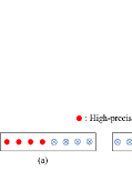
Fig. 1: Different mixed-ADC arrangements using ULA

In this work, we derive the CRB associated with DOA under the mixed-ADC based architecture with time-varying threshold. For computational simplicity, we consider the asymptotic CRB and find it is related to the arrangement of high-precision and one-bit ADCs. Furthermore, we propose a new concept named “mixed-precision arrangement”. It is found that the high-precision ADCs should be arranged evenly around the edges of the ULA to achieve a lower CRB like the case in Fig. 1(c). Numerical results demonstrate that the asymptotic CRB is valid and the optimal mixed-precision arrangement can achieve better performance.

Notation: We denote vectors and matrices by bold lowercase and uppercase letters, respectively. $(\cdot)^{T}$ and $(\cdot)^{H}$ represent the transpose and the conjugate transpose, respectively. $\mathbf{I}_{N}$ denotes an $N\times N$ identity matrix and $\mathbf{1}_{N}=[1,\ldots,1]^{T}\in\mathbb{R}^{N\times 1}$. $\otimes$, $\odot$ and $\circ$ denote the Kronecker, Khatri–Rao and Hadamard matrix products, respectively. $\rm{vec}(\cdot)$ refers to the column-wise vectorization operation and $\rm{diag}(\mathbf{d})$ denotes a diagonal matrix with diagonal entries formed from $\mathbf{d}$. $\mathbf{A}_{\mathrm{R}}\triangleq\Re\{\mathbf{A}\}$ and $\mathbf{A}_{\mathrm{I}}\triangleq\Im\{\mathbf{A}\}$, where $\Re\left\{\cdot\right\}$ and $\Im\left\{\cdot\right\}$ denote the real and imaginary parts, respectively. $\mathrm{sign}(\cdot)$ is the sign function applied element-wise to vector or matrix and $\lfloor\cdot\rfloor$ is the floor function. Finally, $j\triangleq\sqrt{-1}$.

2 Signal Model

We consider $K$ narrowband far-field signals impinging on a ULA with $M$ elements from different directions $\{\theta_{1},\dots,\theta_{K}\}$. After sampling, the array output can be stacked over the whole $N$ snapshots as

$$\mathbf{X}=\mathbf{A}\mathbf{S}+\mathbf{E},$$ (1)

where     $\mathbf{X}=[\mathbf{x}(1),\mathbf{x}(2),\dots,\mathbf{x}(N)]\in\mathbb{C}^{M\times N}$     is the received signal matrix, $\mathbf{A}=\left[\mathbf{a}\left(\theta_{1}\right),\cdots,\mathbf{a}\left(\theta_{K}\right)\right]\in\mathbb{C}^{M\times K}$ represents the array steering matrix with $\mathbf{a}(\theta_{k})$ denoting the steering vector associated with $k$th source, $\mathbf{S}=[\mathbf{s}(1),\mathbf{s}(2),\dots,\mathbf{s}(N)]\in\mathbb{C}^{K\times N}$ denotes the source signal matrix, and $\mathbf{E}=[\mathbf{e}(1),\mathbf{e}(2),\dots,\mathbf{e}(N)]\in\mathbb{C}^{M\times N}$ is the noise sequence. The noise has the zero-mean circularly symmetric complex-valued white Gaussian distribution with independent and identically distributed (i.i.d.) known variance $\sigma^{2}$. Under the case of ULA with half-wavelength antenna spacing , the steering vector $\mathbf{a}(\theta_{k})$ can be written as

$$\mathbf{a}(\theta_{k}) =\begin{bmatrix}1,e^{j\pi\sin\theta_{k}},\dots,e^{j\pi(M-1)\sin\theta_{k}}\end{bmatrix}^{T}.$$ (2)

The source signal matrix $\mathbf{S}$ is assumed to be deterministic but unknown, which is referred to as the conditional or deterministic model [15].

When one-bit ADC is employed with time-varying threshold for quantization, the array output is modified as

$$\mathbf{Z}=\mathcal{Q}(\mathbf{X}-\mathbf{H}),$$ (3)

where $\mathbf{H}\in\mathbb{C}^{M\times N}$ represents the known threshold and $\mathcal{Q}(\cdot)=\mathrm{sign}(\Re\{\cdot\})+j\mathrm{sign}(\Im\{\cdot\})$ denotes the complex one-bit quantization operator.

We consider a mixed-ADC based architecture equipped with $M_{0}$ high-resolution ADCs and $M_{1}$ one-bit ADCs, where $M_{0}+M_{1}=M$. More generally, we define a high-precision ADC indicator vector $\bm{\delta}=[\delta_{1},\dots,\delta_{M}]^{T}$ with $\delta_{i}\in\{0,1\}$, which means that the $i$th antenna is equipped with high-precision ADC when $\delta_{i}=1$ and one-bit ADC when $\delta_{i}=0$. So the mixed output can be represented as

$$\mathbf{Y}=\mathbf{Z}\circ(\bm{\bar{\delta}}\otimes\mathbf{1}_{N}^{T})+\mathbf{X}\circ(\bm{\delta}\otimes\mathbf{1}_{N}^{T}),$$ (4)

where $\bm{\bar{\delta}}=\mathbb{1}_{M}-\bm{\delta}$ is the indicator for one-bit ADC.

3 Cramér-Rao Bounds for Mixed Data

Let $\bm{\varphi}$ collect all the real-valued unknown target parameters, i.e., $\bm{\varphi}=\begin{bmatrix}\bm{\theta}^{T},\ \mathbf{s}_{\rm R}^{T},\ \mathbf{s}_{\rm I}^{T}\end{bmatrix}^{T}\in\mathbb{R}^{(K+2KN)\times 1}$, where $\mathbf{s}=\rm{vec}(\mathbf{S})$.

In [13], it is proved that the Fisher information matrix (FIM) for mixed-ADC data is the summation of the FIMs for the high-precision data and one-bit data, i.e.,

$$\mathbf{F}_{m}(\bm{\varphi})=\mathbf{F}_{0}(\bm{\varphi})+\mathbf{F}_{1}(\bm{\varphi}),$$ (5)

where $\mathbf{F}_{0}(\bm{\varphi})$ and $\mathbf{F}_{1}(\bm{\varphi})$ are FIMs for high-precision data and one-bit data, respectively.

Let the derivatives of the high-precision and one-bit data with respect to $\bm{\varphi}$ denote as:

$$\mathbf{U}_{0} =\mathbf{U}\text{diag}\left(\mathbf{1}_{N}\otimes\bm{\delta}\right),$$

$$\mathbf{U}_{1} =\mathbf{U}\text{diag}\left(\mathbf{1}_{N}\otimes\overline{\bm{\delta}}\right),$$ (6)

respectively, where

$$\mathbf{U}=\left[\mathbf{\Delta},\quad\mathbf{G},\quad j\mathbf{G}\right]^{H},$$ (7)

$$\mathbf{\Delta}=\mathbf{S}^{T}\odot\dot{\mathbf{A}},\quad\mathbf{G}=\mathbf{I}_{N}\otimes\mathbf{A},$$ (8)

$$\dot{\mathbf{A}}=\left[\frac{\partial\mathbf{a}\left(\theta_{1}\right)}{\partial\theta_{1}},\ldots,\frac{\partial\mathbf{a}\left(\theta_{K}\right)}{\partial\theta_{K}}\right].$$ (9)

From [16, 17] and (5), the FIM for mixed data can be written as

$$\mathbf{F}_{m}(\bm{\varphi})= \frac{2}{\sigma^{2}}\Re\left\{\mathbf{U}_{0}\mathbf{U}_{0}^{H}\right\}$$

$$+\frac{1}{\pi\sigma^{2}}\left(\mathbf{U}_{1,\rm R}\bm{\Lambda}_{\rm R}\mathbf{U}_{1,\rm R}^{T}+\mathbf{U}_{1,\rm I}\bm{\Lambda}_{\rm I}\mathbf{U}_{1,\rm I}^{T}\right),$$ (10)

where $\mathbf{\Lambda}=\text{diag}([\lambda_{1},\ldots,\lambda_{MN}])$ . The diagonal element $\lambda_{k}$ in $\mathbf{\Lambda}$ is given by

$$\lambda_{k}=B\left(\frac{\Re\left(\zeta_{k}\right)}{\sigma/\sqrt{2}}\right)+jB\left(\frac{\Im\left(\zeta_{k}\right)}{\sigma/\sqrt{2}}\right),$$ (11)

where $\zeta_{k}$ is the $k$th element in $\bm{\zeta}=\text{vec}(\mathbf{A}\mathbf{S}-\mathbf{H})\in\mathbb{C}^{MN\times 1}$ and the function $B(\cdot)$ is defined by

$$B(x)=\left[\frac{1}{\Phi(x)}+\frac{1}{\Phi(-x)}\right]e^{-x^{2}}$$ (12)

with $\Phi(x)=\int_{-\infty}^{x}\frac{1}{\sqrt{2\pi}}e^{-\frac{t^{2}}{2}}dt$ being the cumulative distribution function of the normal standard distribution.

Considering the optimal time-varying threshold, i.e., $\mathbf{H}=\mathbf{A}\mathbf{S}$, the FIM for mixed-ADC data can be simplified as

$$\mathbf{F}_{m}(\bm{\varphi}) =\frac{2}{\sigma^{2}}\Re\left\{\mathbf{U}_{0}\mathbf{U}_{0}^{H}\right\}+\frac{4}{\pi\sigma^{2}}\left(\mathbf{U}_{1,\rm R}\mathbf{U}_{1,\rm R}^{T}+\mathbf{U}_{1,\rm I}\mathbf{U}_{1,\rm I}^{T}\right)$$

$$=\frac{2}{\sigma^{2}}(\mathbf{U}_{\rm R}\bar{\mathbf{\Sigma}}\mathbf{U}_{\rm R}^{T}+\mathbf{U}_{\rm I}\bar{\mathbf{\Sigma}}\mathbf{U}_{\rm I}^{T}),$$ (13)

where

$$\bar{\bm{\Sigma}}=\mathbf{I}_{N}\otimes\mathbf{\Sigma}_{0},\quad\bm{\Sigma}_{0}=\left(1-\frac{2}{\pi}\right)\text{diag}(\bm{\delta})+\frac{2}{\pi}\mathbf{I}_{M}.$$ (14)

Let $\bar{\mathbf{U}}=\mathbf{U}\bar{\mathbf{\Sigma}}^{\frac{1}{2}}$, we have $\bar{\mathbf{U}}=[\bar{\mathbb{\Delta}},\quad\bar{\mathbf{G}},\quad j\bar{\mathbf{G}}]^{H}$, where

$$\bar{\mathbf{\Delta}}=\bar{\mathbf{\Sigma}}^{\frac{1}{2}}\mathbf{\Delta},\quad\bar{\mathbf{G}}=\mathbf{I}_{N}\otimes(\mathbf{\Sigma}_{0}^{\frac{1}{2}}\mathbf{A}).$$ (15)

Finally, we can concisely write the FIM for mixed-ADC data as

$$\mathbf{F}_{m}(\bm{\varphi}) =\frac{2}{\sigma^{2}}\Re\left\{\bar{\mathbf{U}}\bar{\mathbf{U}}^{H}\right\}.$$ (16)

Following the approach given in [16], we can obtain the DOA-related block of the deterministic CRB by block-wise inversion, i.e.,

$$\mathbf{CRB}(\mathbf{\theta})=\frac{\sigma^{2}}{2}\Re\left\{\bar{\mathbf{\Delta}}^{H}\mathbf{\Pi}_{\bar{\mathbf{G}}}^{\perp}\bar{\mathbf{\Delta}}\right\}^{-1},$$ (17)

where $\mathbb{\Pi}_{\bar{\mathbf{G}}}^{\perp}=\mathbf{I}-\bar{\mathbf{G}}\left(\bar{\mathbf{G}}^{H}\bar{\mathbf{G}}\right)^{-1}\bar{\mathbf{G}}^{H}$ is the orthogonal projector onto the null space of $\bar{\mathbf{G}}^{H}$. Substituting (15) into (17), we have a more clear expression for the CRB:

$$\mathbf{CRB}(\mathbf{\theta})=\frac{\sigma^{2}}{2N}\Re\left\{\left(\dot{\mathbf{A}}^{H}\mathbf{\Omega}\dot{\mathbf{A}}\right)\circ\hat{\mathbf{P}}^{T}\right\}^{-1},$$ (18)

where

$$\hat{\mathbf{P}} =\frac{1}{N}\sum_{t=1}^{N}\mathbf{s}(t)\mathbf{s}^{H}(t),$$ (19)

$$\mathbf{\Omega} =\mathbb{\Sigma}_{0}-\mathbb{\Sigma}_{0}\mathbf{A}(\mathbf{A}^{H}\mathbb{\Sigma}_{0}\mathbf{A})^{-1}\mathbf{A}^{H}\mathbb{\Sigma}_{0}.$$ (20)

3.1 CRB for $K=1,N=1$

When the target and snapshot are both single, the CRB associated with DOA is given as

$$\mathrm{CRB}(\theta)=\frac{\sigma^{2}(M_{0}+\frac{2}{\pi}M_{1})}{2pS\pi^{2}\cos^{2}\theta}=\frac{M_{0}+\frac{2}{\pi}M_{1}}{2\pi^{2}S}\frac{1}{\text{SNR}\cos^{2}\theta},$$ (21)

where $p$ is the signal power, $\text{SNR}=\frac{p}{\sigma^{2}}$ and

$$S=\sum_{i=1}^{M}g_{i}(i-1)^{2}\sum_{i=1}^{M}g_{i}-\left[\sum_{i=1}^{M}g_{i}(i-1)\right]^{2},$$ (22)

in which $g_{i}\in\{1,\frac{2}{\pi}\}$, $\sum_{i=1}^{M}g_{i}=M_{0}+\frac{2}{\pi}M_{1}$, and $M_{0}+M_{1}=M$.

3.2 Asymptotic CRB

For sufficiently large $N$, the estimated power $\hat{\mathbf{P}}$ can be replaced by the true power $\mathbf{P}$. Thus, the CRB is given by

$$\mathbf{CRB}(\mathbf{\theta})=\frac{\sigma^{2}}{2N}\Re\left\{\left(\dot{\mathbf{A}}^{H}\mathbf{\Omega}\dot{\mathbf{A}}\right)\circ\mathbf{P}^{T}\right\}^{-1}.$$ (23)

When $M$ is sufficiently large, and the number of high-precision ADC is assumed to be constrained (i.e., $M_{1}$ does not increase proportionally with $M$). We can obtain the following asymptotic result:

$$\mathbf{CRB}(\mathbf{\bm{\theta}})=\frac{M_{0}+\frac{2}{\pi}M_{1}}{2\pi^{2}NS}\left[\begin{array}[]{lll}\frac{1}{\text{SNR}_{1}\cos^{2}\theta_{1}}&&0\\ &\ddots&\\ 0&&\frac{1}{\text{SNR}_{K}\cos^{2}\theta_{K}}\end{array}\right],$$ (27)

where $\text{SNR}_{i}$ is the signal-to-noise ratio for the $i$th signal. This result is motivated by (21) and [18], and its detailed derivation can be seen in [19].

It is worth mentioning that the CRB in (21) and (27) for the mixed-ADC associated with DOA is concerned with the arrangement of the high-precision and one-bit ADCs (i.e., how to maximize $S$), which is rarely mentioned in the previous. We will study the problem in Section 4.

4 Analysis of Arrangement in the Mixed-ADC Based Architecture

Considering the problem mentioned in the last section, the CRB above is achievable using maximum likelihood estimation. So we can get better estimation for DOA if we properly design the arrangement of high-precision and one-bit ADCs. Intuitively, using Lagrange’s identity, we can reformulate the optimization problem as

$$\max_{\{g_{i}\}_{i=1,2\cdots,M}}\quad S=\sum_{i=1}^{M}\sum_{j>i}g_{i}g_{j}(j-i)^{2}$$

$$\ \ {\rm s.t.}\quad g_{i}\in\{1,\frac{2}{\pi}\},\quad i=1,2,\dots,M,$$

$$\qquad\quad\ \sum_{i=1}^{M}g_{i}=M_{0}+\frac{2}{\pi}M_{1},$$ (28)

which is called the mixed-precision arrangement problem.

Proposition 1.

The solution to (4) is that the high-precision ADCs are placed evenly around the edges of the ULA.

Proof.

We adopt the strategy swapping the positions of the high-precision and one-bit ADCs to achieve the optimal arrangement. Generally, let $\tilde{S}(\tilde{g}_{m}=1,\tilde{g}_{n}=\frac{2}{\pi},\dots)$ denote the arrangement that the positions of the $m$th and $n$th ADCs are swapped based on $S(g_{m}=\frac{2}{\pi},g_{n}=1,\dots)$ and $M_{h}=\lfloor\frac{M_{0}+1}{2}\rfloor$. We consider two special cases. The first case is $m\leq M_{h}$ and $m$ is the first one-bit ADC’s index from left to right. The second is $m\geq M-M_{h}+1$ and $m$ is the first one-bit ADC’s index from right to left. In both cases, $n$ is the index of the first high precision ADC appears from the $m$th to the other side.

Note that $S$ can be written as

$$S= g_{m}\sum_{j=1,j\neq m,n}^{M}g_{j}(j-m)^{2}+g_{n}\sum_{j=1,j\neq m,n}^{M}g_{j}(j-n)^{2}$$

$$+g_{m}g_{n}(m-n)^{2}+C,$$ (29)

where the constant $C$ is not related to $m$ or $n$. Similarly, we have

$$\tilde{S}-S=\left(1-\frac{2}{\pi}\right)(n-m)\sum_{j=1,j\neq m,n}^{M}g_{j}(2j-m-n).$$ (30)

Let $H(m,n)\triangleq\sum_{j=1,j\neq m,n}^{M}g_{j}(2j-m-n)$. Note that $H(m,n)$ has no change if we let $g_{m}=g_{n}=1$. It can be expressed as

$$H(m,n)=2\sum_{j=1}^{M}g_{j}j-(m+n)\sum_{j=1}^{M}g_{j}$$

$$\geq 2\sum_{j=1}^{m}j+\frac{4}{\pi}\sum_{j=m+1}^{n-1}j+2\sum_{j=n}^{n+M_{0}-m}j$$

$$+\frac{4}{\pi}\sum_{j=n+M_{0}-m+1}^{M}j-(m+n)\sum_{j=1}^{M}g_{j}\triangleq H^{\prime}(m,n).$$ (31)

In the first case, using the facts $0<m\leq M_{h}$ and $m<n\leq M_{h}+M_{1}$, we obtain that

$$H^{\prime}(m,n)-H^{\prime}(m+1,n)$$

$$=(1-\frac{2}{\pi})(2n+3M_{0}-4m-1)+\frac{2}{\pi}M$$

$$\geq(1-\frac{2}{\pi})(3M_{0}-2M_{h}+1)+\frac{2}{\pi}M>0,$$ (32)

and

$$H^{\prime}(m,n)-H^{\prime}(m,n+1)$$

$$=(1-\frac{2}{\pi})(2m-M_{0}+1)+\frac{2}{\pi}M$$

$$>\frac{2}{\pi}M-(1-\frac{2}{\pi})M_{1}>(1-\frac{2}{\pi})M_{0}>0.$$ (33)

Combining the above inequality, we have

$$H(m,n)\geq H^{\prime}(m,n)\geq H^{\prime}(M_{h},M_{h}+M_{1})$$

$$=M(M_{0}-2M_{h}+1)+\frac{2}{\pi}(2M_{h}+M_{1})$$

$$=\left\{\begin{array}[]{rcl}(1+\frac{2}{\pi})M&&M_{0}\quad\text{is even}\\ \frac{2}{\pi}(M+1)&&M_{0}\quad\text{is odd}\end{array}\right.>0.$$ (36)

So it is proved that $\tilde{S}>S$ in the first case.

In the second case, by letting $j^{\prime}=M+1-j$, we have

$$H(m,n) =2\sum_{j=1}^{M}g_{j}(M+1-j^{\prime})-(2M+2-m^{\prime}-n^{\prime})\sum_{j=1}^{M}g_{j}$$

$$=(m^{\prime}+n^{\prime})\sum_{j=1}^{M}g_{j}-2\sum_{j=1}^{M}g_{j}j^{\prime}.$$ (37)

Due to the fact $m^{\prime}\leq M_{h}$, it is same as the first case. In summery, we have $\tilde{S}>S$ in both cases.

Therefore, we can adjust the positions of high-precision and one-bit ADCs in steps to maximize $S$ until none of the above situations exist. Finally, the high-precision ADCs are distributed evenly around the edges of the ULA like Fig. 1(c), which is the optimal mixed-precision arrangement. ∎

Remark 1.

Note that Proposition 1 can be extended to a more complex scenarios that the ULA is equipped with various precision ADCs. Combining the fact that the CRB decreases as the quantization becomes increasingly finer [20], the higher precision ADCs should be placed from center as far as possible to achieve better performance (see more details in [19]).

5 Simulation and Discussion

In this section, we present numerical examples to demonstrate the effectiveness of the asymptotic CRB and the optimal mixed-precision arrangement. Assuming the ULA spaced at $d=\frac{1}{2}\lambda$ with $M=30$ and $M_{0}=10$, we consider three situations showed in Fig. 1 for the mixed-ADC based architecture:

1. $\{\delta_{i}=1\}_{i=1}^{10}$ and $\{\delta_{i}=0\}_{i=11}^{30}$ like Fig. 1(a);

2. $\{\delta_{i}=0\}_{i=1}^{10}$, $\{\delta_{i}=1\}_{i=11}^{20}$ and $\{\delta_{i}=0\}_{i=21}^{30}$ like Fig. 1(b);

3. $\{\delta_{i}=1\}_{i=1}^{5}$, $\{\delta_{i}=0\}_{i=6}^{25}$ and $\{\delta_{i}=1\}_{i=26}^{30}$, which is the optimal mixed-precision arrangement like Fig. 1(c) that high-precision ADCs are distributed evenly around the edges.

We consider two targets with $\theta_{1}=10^{\circ},\theta_{2}=20^{\circ},p_{1}=p_{2}=1$. For the one-bit ADC system and mixed-ADC based architecture, the time-vary threshold has the real and imaginary parts selected randomly and equally likely from a predefined eight-element set $\{-h_{\text{max}},-h_{\text{max}}+\Delta,\dots,h_{\text{max}}-\Delta,h_{\text{max}}\}$ with $h_{\text{max}}=2$ and $\Delta=\frac{h_{\text{max}}}{7}$.

Fig. 2 shows the CRBs versus $N$ and SNR for $\theta_{1}$ where situations 1, 2 and 3 are denoted as “Mixed-ADC1”, “Mixed-ADC2” and “Mixed-ADC3”, respectively. Compared with the one-bit system, the mixed-ADC based architectures can achieve significant performance improvements, especially for the “Mixed-ADC3” with large SNR.

When $\text{SNR}=-20$ dB, the optimal threshold can be closed to that by using time-varying threshold scheme. Fig. 2(a) shows that the CRBs for mixed-ADC data almost coincide with the asymptotic CRB. Also, the optimal mixed-precision arrangement has lower CRB than others. It is shown in Fig. 2(b) that when the SNR changes, the optimal mixed-precision arrangement has better performance than others on both asymptotic CRB and actual CRB with time-varying thresholds. In particular, the CRB of the optimal mixed-precision arrangement is almost $10$ dB lower than others, when the SNR is large. Hence, it is inappropriate to take a random mixed-precision arrangement given the number of high-precision and one-bit ADCs, which may cause a large performance loss especially in the high SNR regime.

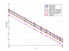
(a) CRB versus $N$, $\text{SNR}=-20$ dB

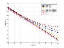
(b) CRB versus SNR, $N=10$

Fig. 2: CRB versus $N$ and SNR

6 Conclusions

In this work, we have considered the mixed-ADC based architecture for DOA estimation using ULA. We have derived the CRB associated with DOA under the optimal time-vary threshold. We found the asymptotic CRB is related to the arrangement of high-precision and one-bit ADC. Based on it, we have proved that the high-precision ADCs should be distributed evenly around the edges of ULA to achieve a lower CRB. It can be extended to more general case where the ULA is equipped with various precision ADCs.

References

- [1] E. Tuncer and B. Friedlander, Classical and modern direction-of-arrival estimation, Academic Press, 2009.
- [2] S. Sun, A. P. Petropulu, and H. V. Poor, “MIMO radar for advanced driver-assistance systems and autonomous driving: Advantages and challenges,” IEEE Signal Process. Mag., vol. 37, no. 4, pp. 98–117, 2020.
- [3] H. Krim and M. Viberg, “Two decades of array signal processing research: The parametric approach,” IEEE Signal Process. Mag., vol. 13, no. 4, pp. 67–94, 1996.
- [4] R. H. Walden, “Analog-to-digital converter survey and analysis,” IEEE J. Sel. Areas Commun., vol. 17, no. 4, pp. 539–550, 1999.
- [5] O. Bar-Shalom and A. J. Weiss, “DOA estimation using one-bit quantized measurements,” IEEE Trans. Aerosp. Electron. Syst., vol. 38, no. 3, pp. 868–884, 2002.
- [6] A. Ameri, A. Bose, J. Li, and M. Soltanalian, “One-bit radar processing with time-varying sampling thresholds,” IEEE Trans. Signal Process., vol. 67, no. 20, pp. 5297–5308, 2019.
- [7] B. Zhao, L. Huang, J. Li, M. Liu, and J. Wang, “Deceptive SAR jamming based on 1-bit sampling and time-varying thresholds,” IEEE J. Sel. Topics Appl. Earth Observ. Remote Sens., vol. 11, no. 3, pp. 939–950, 2018.
- [8] A. Eamaz, F. Yeganegi, and M. Soltanalian, “Covariance recovery for one-bit sampled non-stationary signals with time-varying sampling thresholds,” IEEE Trans Signal Process., vol. 70, pp. 5222–5236, 2022.
- [9] A. Eamaz, F. Yeganegi, and M. Soltanalian, “Modified arcsine law for one-bit sampled stationary signals with time-varying thresholds,” in Proc. IEEE Int. Conf. Acoust., Speech Signal Process., Toronto, Ontario, Canada, Jun., pp. 5459–5463.
- [10] J. Mo and R. W. Heath, “High SNR capacity of millimeter wave MIMO systems with one-bit quantization,” in Proc. Inf. Theory Appl. Workshop, San Diego, CA, USA, Feb. 2014, pp. 1–5.
- [11] N. Liang and W. Zhang, “Mixed-ADC massive MIMO,” IEEE J. Sel. Areas Commun., vol. 34, no. 4, pp. 983–997, 2016.
- [12] B. Shi, L. Zhu, W. Cai, N. Chen, T. Shen, P. Zhu, F. Shu, and J. Wang, “On performance loss of DOA measurement using massive MIMO receiver with mixed-ADCs,” IEEE Wireless Commun. Lett., 2022.
- [13] X. Shang, R. Lin, and Y. Cheng, “Mixed-ADC based PMCW MIMO radar angle-doppler imaging,” submmited to IEEE Trans. Signal Process., 2022.
- [14] Y. Cheng, X. Shang, and F. Liu, “CRB analysis for mixed-ADC PMCW MIMO Radar,” in Proc. CIE Int. Conf. Radar, Hai Kou, China, Dec. 2021, pp. 1032–1037.
- [15] P. Stoica and A. Nehorai, “Performance study of conditional and unconditional direction-of-arrival estimation,” IEEE Trans. Acoust., Speech, Signal Process., vol. 38, no. 10, pp. 1783–1795, Oct. 1990.
- [16] P. Stoica and R. L. Moses, Spectral analysis of signals, vol. 452, Pearson Prentice Hall Upper Saddle River, NJ, 2005.
- [17] C. Li, R. Zhang, J. Li, and P. Stoica, “Bayesian information criterion for signed measurements with application to sinusoidal signals,” IEEE Signal Process. Lett., vol. 25, no. 8, pp. 1251–1255, 2018.
- [18] P. Stoica and A. Nehorai, “MUSIC, maximum likelihood, and Cramér-Rao bound,” IEEE Trans. Acoust., Speech, Signal Process., vol. 37, no. 5, pp. 720–741, 1989.
- [19] X. Zhang and Y. Cheng, “Location arrangement optimization and DOA estimation for mixed-ADC using ULA,” to be submmitted.
- [20] P. Stoica, X. Shang, and Y. Cheng, “The Cramér–Rao bound for signal parameter estimation from quantized data [Lecture Notes],” IEEE Signal Process. Mag., vol. 39, no. 1, pp. 118–125, 2022.