DANI-Net: Uncalibrated Photometric Stereo by Differentiable Shadow Handling, Anisotropic Reflectance Modeling, and Neural Inverse Rendering

Abstract

Uncalibrated photometric stereo (UPS) is challenging due to the inherent ambiguity brought by the unknown light. Although the ambiguity is alleviated on non-Lambertian objects, the problem is still difficult to solve for more general objects with complex shapes introducing irregular shadows and general materials with complex reflectance like anisotropic reflectance. To exploit cues from shadow and reflectance to solve UPS and improve performance on general materials, we propose DANI-Net, an inverse rendering framework with differentiable shadow handling and anisotropic reflectance modeling. Unlike most previous methods that use non-differentiable shadow maps and assume isotropic material, our network benefits from cues of shadow and anisotropic reflectance through two differentiable paths. Experiments on multiple real-world datasets demonstrate our superior and robust performance.

1 Introduction

Photometric stereo (PS) [48] aims at recovering the surface normal from several images captured under varying light conditions with a fixed viewpoint. It has been applied to many fields (e.g., movies production [6], industrial quality inspection [47], and biometrics [53]) due to its advantage in recovering fine-detailed surfaces over other approaches [16, 10] (e.g., multi-view stereo [38], active sensor-based solutions [61]). Light calibration is crucial to the performance [52]. However, it is also tedious, restricting the applicability of PS. Therefore, uncalibrated photometric stereo (UPS) methods estimating surface normal with unknown lights have been widely studied in the literature.

Uncalibrated photometric stereo suffers from General Bas-Relief (GBR) ambiguity [4] for an integrable, Lambertian surface. However, GBR ambiguity is alleviated on a non-Lambertian surface [13]. Therefore, recent advances in UPS (e.g., [26, 56]) adopt the isotropic reflectance model accounting for non-Lambertian effects to solve UPS. Nonetheless, such a model restricts methods’ performance on objects with more general (e.g., anisotropic) materials, while modeling general reflectance is challenging due to extra unknowns, which eventually make UPS intractable. Other works (e.g., [25, 57, 56]) notice the benefits of the shadow cues in utilizing global shape-light information to solve PS/UPS because the shadow reflects the interaction of shape and light [59, 24]. However, these methods either fail to exploit the shadow cues due to the lack of a differentiable path from the shadow to the concerned unknowns like shape [25], or the shadow cues have limited effects on the visible shape reconstruction due to the implicit shape representation [57, 56].

To this end, this paper proposes the DANI-Net, which solves UPS by Differentiable shadow handling, Anisotropic reflectance modeling, and Neural Inverse Rendering. DANI-Net builds the differentiable path in the sequence of inverse rendering errors, shadow maps, and surface normal maps (or light conditions) (Fig. 1) to fully exploit the shadow cues to solve UPS. Since those cues facilitate solving extra unknowns introduced by a more sophisticated reflectance model, DANI-Net manages to build up such a model (Fig. 1) to improve the performance on general materials. During optimization, DANI-Net propagates inverse rendering errors via two paths of shadow cues and anisotropic reflectance, respectively, and simultaneously optimizes the shape (i.e., the depth map and surface normal map), anisotropic reflectance model, shadow map, and light conditions (i.e., direction and intensity). As a result, DANI-Net achieves state-of-the-art performance on several real-world benchmark datasets. In a nutshell, our contributions are summarized as follows:

• We propose a differentiable shadow handling method that facilitates exploiting shadow cues with global shape-light information to solve UPS. Experimental results demonstrate its effectiveness in shadow map recovery and surface normal estimation.

• We introduce an anisotropic reflectance model that describes both isotropic and anisotropic materials to improve performance on general materials. Experimental results demonstrate its effectiveness on surface normal estimation for objects with a broad range of isotropic and anisotropic materials.

• We propose the DANI-Net that simultaneously optimizes shape, anisotropic reflectance, shadow map, and light conditions in an unsupervised manner, propagating inverse rendering errors through two paths involving the shadow cues and anisotropic reflectance, respectively. DANI-Net achieves state-of-the-art performance on several real-world benchmark datasets.

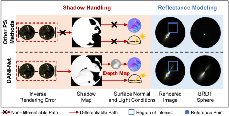
Figure 1: The proposed DANI-Net differs from other PS or UPS methods in two aspects: 1) Shadow Handling. The path in the sequence of inverse rendering errors, shadow maps, and surface normal maps (or light conditions) of the DANI-Net is differentiable; 2) Reflectance Modeling. DANI-Net adopts an anisotropic reflectance model. The state-of-the-art UPS method SCPS-NIR [26] is compared in this figure. As can be observed, the proposed DANI-Net produces a smoother and more realistic shadow map of copper Bunny thanks to the differentiable shadow handling and renders a more realistic copper Ball image and Bidirectional Reflectance Distribution Function (BRDF) sphere (of the reference point) due to the anisotropic reflectance modeling. Data of copper Bunny and Ball are from DiLiGenT$10^{2}$ [36].

2 Related Work

This section reviews the relevant works in PS. Table 1 summarizes differences between representative existing PS methods and the proposed DANI-Net. We also briefly review recent advances in neural reflectance representation in 3D vision. Note that our reviews on calibrated PS only include the unsupervised calibrated PS methods. Readers may refer to [40, 54, 65] for more summaries on supervised PS methods and neural reflectance representation methods.

Unsupervised calibrated photometric stereo. The baseline method (LS [48]) assumes Lambertian surface and solves PS via least squares optimization. A category of traditional methods considers the non-Lambertian reflectance as outliers [3, 12, 49, 50]. Another category of traditional methods either adopt analytic models (e.g., Torrance-Sparrow [13], Ward [12, 14, 1], Bi-polynomial [64], etc.) or utilize the general reflectance features (e.g., isotropy [2], monotonicity [17], anisotropic properties [14, 18]). Traditional methods rely on optimizers tailored to specific assumptions, making them computationally efficient but less accurate. In contrast, although learning-based approaches are more computationally demanding, they could offer superior performance on general objects. Recently, a group of learning-based unsupervised methods (TM18 [43] and LL22 [25]) has been proposed to estimate the spatially varying BRDFs and the surface normal with known lights.

Uncalibrated photometric stereo. Early works either hold the Lambertian assumption and exploit extra clues from reflectance [28, 39, 58] or make additional assumptions of light source distribution [66, 39, 51, 34, 28] to alleviate GBR ambiguity [4] in UPS. Supervised methods (CH19 [8], CW20 [10], and SK22 [37]) achieve promising performance on public benchmark datasets. However, these methods assume the light intensity distributing in a pre-defined range (i.e., $[0.2,2]$) and solve UPS in two-stage, making them suffer from the data bias (between synthetic training data and real-world ones) and the accumulating errors. Recently, SCPS-NIR [26] utilizes the neural inverse rendering method to jointly optimize light and surface normal in an unsupervised manner based on local reflectance information, free from data bias and accumulating errors. The proposed DANI-Net also addresses UPS in an unsupervised manner, but it differs from all previous works in two aspects. 1) Our method builds a differentiable path in the sequence of inverse rendering errors, shadow maps, and surface normal maps (or light conditions), which fully exploits shadow cues containing global shape-light information to solve UPS. 2) Our method introduces the anisotropic reflectance model in solving UPS, which improves the performance on general materials. Besides, as compared with [26] that calculates shadow maps by image binarization and fixes them during training, our method computes shadow maps from shapes and constantly updates them during training.

Shadow handling in photometric stereo. Supervised learning-based methods [8, 10, 37] handle shadow implicitly by learning priors from training data, while unsupervised ones often consider the shadow as the outliers (e.g., [48, 43, 34, 60, 25, 26]). Aware of useful cues in the shadow, several works utilize the shadow information explicitly by involving the shadow in inverse rendering to solve PS/UPS. However, early works [7, 42] assume Lambertian surface, which restricts them to general materials, while recent advances (LL22 [25], SCPS-NIR [26], S3-NeRF [57], KF22 [23], PS-NeRF [56]) fail to efficiently exploit shadow cues. That is, some works [26, 25] calculate the shadow map without simultaneously optimizing shadow and other unknowns due to the discontinuity of the binary representation of the shadow map; the others either need the ground truth of shadow maps and ignore the shading cue [23], or rely on priors of scene or light to ensure the accuracy [57, 56]. In contrast, DANI-Net simultaneously optimizes shadow and other unknowns, and exploits shadow and reflectance cues for UPS.

Neural reflectance representation in 3D vision. Neural Radiance Fields (NeRFs) [29] implicitly represent the shape information through MLPs. While NeRF [29] applies volume rendering [22] to optimize the MLPs through reconstruction loss, they often end up with ‘fake reflectance’ [44] (i.e., the emitters inside the objects contribute to specific reflectance effects) and inaccurate geometries due to the lack of an implicit surface representation [54]. To solve this, works like [46, 32] combine surface rendering [21] with volume rendering [22]. Other works [44, 63, 62, 5, 41] adopt explicit representation on surface’s reflectance to mimic realistic reflectance, which improves the accuracy of NeRF [29]. Different from the above methods that work on multi-view inputs and focus on the full but coarse geometry recovery, DANI-Net takes single-view inputs under a UPS setup and focuses on the fine-detailed recovery of depth and surface normal.

Table 1: A summary of differences between the proposed DANI-Net and representative existing PS and UPS methods in terms of the solving problem, supervision, shadow handling strategy, and material model. We categorize the shadow handling strategy as ‘outliers’ rather than ‘cues’, if it models the shadow without explicitly exploiting it for shape recovery. ‘N.A.’ represents Not Applicable.

Method	Problem	Supervision	Shadow Handling	Material Model
TM18 [43]	PS	Unsupervised	Implicit (Outliers)	Isotropic (Bi-Polynomial BRDFs)
LL22 [25]	PS	Unsupervised	Non-differentiable (Outliers)	Isotropic (MLP Bases)
CH19 [8]	UPS	Light + Surface Normal	Implicit (Data-driven)	Implicit (Data-driven)
CW20 [10]	UPS	Light + Surface Normal	Implicit (Data-driven)	Implicit (Data-driven)
CM20 [11]	Semi-PS	Unsupervised	$\ell_{1}$-based Minimization (Outliers)	Lambertian
SK22 [37]	UPS	Light + Surface Normal	Implicit (Data-driven)	Implicit (Data-driven)
SCPS-NIR [26]	UPS	Unsupervised	Image Binarization (Outliers)	Isotropic (Gaussian Bases)
S3-NeRF [57]	Near Field PS	Unsupervised	Differentiable (Cues for Invisible Shape)	Isotropic (Gaussian Bases)
KF22 [23]	Near Field PS	Unsupervised	Known Shadow Maps (Cues for Visible Shape)	N.A.
DANI-Net	UPS	Unsupervised	Differentiable (Cues for Visible Shape)	Anisotropic (Gaussian Bases)

3 Problem Definition

Following a standard setup of UPS, we take input of a set of observed images $\boldsymbol{I}\triangleq(I_{1},I_{2},...,I_{f})$ of a static object captured under varying directional, parallel lights, and intend to recover light directions $\boldsymbol{L}\triangleq(\boldsymbol{l}_{1},\boldsymbol{l}_{2},...,\boldsymbol{l}_{f})$, light intensities $\boldsymbol{E}\triangleq(e_{1},e_{2},...,e_{f})$, and surface normal $\boldsymbol{N}\triangleq\{\boldsymbol{n}_{i}|i\in\mathbb{P}\}$ based on the observed images, where $\mathbb{P}$ is the set of all positions on the surface. The solution is achieved by solving the optimization problem,

$$\begin{aligned} \mathop{\arg\min}\limits_{\boldsymbol{L},\boldsymbol{E},\boldsymbol{N}}\sum_{i=1}^{\#\mathbb{P}}\sum_{j=1}^{f}{\text{D}(\bar{m}_{ij},m_{ij})},\end{aligned}$$ (1)

where $\bar{m}_{ij}\in I_{j}$ is the observed pixel intensity at position $i$, #$\mathbb{P}$ is the number of elements in $\mathbb{P}$, $\text{D}(\cdot,\cdot)$ is a metric to compute inverse rendering error, $m_{ij}$ is the corresponding rendered pixel intensity. With the linear radiometric response and an orthographic camera, $m_{ij}$ can be formulated as,

$$\begin{aligned} m_{ij}&=e_{j}s_{ij}\rho_{ij}\max(\boldsymbol{n}_{i}^{\top}\boldsymbol{l}_{j},0)\\ &=e_{j}s_{ij}(\rho^{s}_{ij}+\rho^{d}_{ij})\max(\boldsymbol{n}_{i}^{\top}\boldsymbol{l}_{j},0),\end{aligned}$$ (2)

where $\rho_{ij}=\rho(\boldsymbol{n}_{i},\boldsymbol{l}_{j},\boldsymbol{V}_{d})$ describes the general reflectance which contains diffuse $\rho^{d}_{i}$ and specular $\rho^{s}_{ij}$ components, $\boldsymbol{V}_{d}=[0,0,1]$ is the view direction, $\max(\boldsymbol{n}_{i}^{\top}\boldsymbol{l}_{j},0)$ describes the attached shadow, and $s_{ij}$ is the cast shadow calculated from the global shape and light.

Ambiguities in UPS. Unknown light in UPS brings the generalized bas-relief (GBR) ambiguity [4], which can be represented by a $3\times 3$ matrix for the Lambertian surface. For a non-Lambertian surface, specularity helps alleviate the GBR ambiguity [13]. However, general reflectance introduces more unknowns, which require extra cues to solve. Another ambiguity is reflectance-light ambiguity denoted as a non-zero scalar between $e_{j}$ and other terms in Eq. (2). Researchers focus on alleviating the GBR ambiguity while ignoring reflectance-light ambiguity, as the former determines the accuracy of the estimated surface normal. This paper also focuses on alleviating GBR ambiguity.

4 Proposed DANI-Net

This section elaborates on how DANI-Net solves UPS. We first present a differentiable shadow handling method that fully exploits shadow cues to solve UPS and introduces an anisotropic reflectance model that describes a more precise and realistic specularity to improve performance on general materials. We then show how the proposed DANI-Net connects the differentiable shadow handling method, the anisotropic reflectance model, and the inverse rendering together to jointly optimize the shape and light in an unsupervised manner. Finally, we introduce additional loss functions to train DANI-Net.

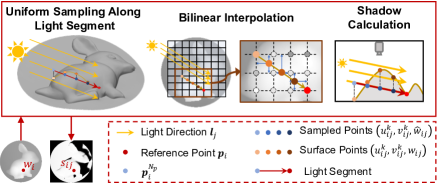
Figure 2: An illustration of our shadow calculation methods, which shows how sampled points and surface points are computed, based on which the shadow is calculated by Eq. (3).

4.1 Differentiable Shadow Handling

Finding the differentiable relationship between shadow, shape, and light is beneficial for solving UPS since 1) it generates a more accurate shadow map through iterative optimization which leads to a more accurate shape-light estimation; 2) compared to previous PS/UPS methods [25, 26] lacking usage of global shape-light information, it facilitates fully exploiting shadow cues containing that information to solve UPS. While the attached shadow is already differentiable to the surface normal and light direction in a specific domain, finding the differentiable relationship for cast shadow is more tricky, since it directly associates with light and the entire depth map instead of the surface normal at a particular point. Such an association raises two key technical challenges to optimizing DANI-Net. First, since the pixel-wise cast shadow calculation increases the computational cost, it is necessary to introduce a technique to improve the training efficiency. Second, since there is no direct connection between the cast shadow and the surface normal, an effective fitting method that calculates the surface normal from the depth map of limited resolution is another required technique to ensure the backpropagation efficiency and the connection from the depth map to the reflectance model for inverse rendering.

Shadow calculation. The basic idea of our shadow calculation method is to consider the occlusion of a reference point according to a few points rather than all points. As shown in Fig. 2, given the depth map $W\triangleq\{w_{i}|1\leq i\leq\#\mathbb{P}\}$, the ‘soft shadow’ [27, 33] $s_{ij}$ of a reference point $\boldsymbol{p}_{i}$ illuminated by a light with direction $\boldsymbol{l}_{j}$ is calculated as:

$${\small\begin{aligned} s_{ij}=\text{Sigmoid}(\alpha(\min\{w^{k}_{ij}-\hat{w}^{k}_{ij}|1\leq k\leq N_{p}\})+\beta),\end{aligned}}$$ (3)

where $\{\hat{w}^{k}_{ij}|1\leq k\leq N_{p}\}$ are depth values of sampled points $\{\boldsymbol{p}_{ij}^{k}|1\leq k\leq N_{p}\}$ uniformly sampled from the light segment that starts at $\boldsymbol{p}_{i}$ along $\boldsymbol{l}_{j}$ and ends at $\boldsymbol{p}_{ij}^{N_{p}}$. $\{{w}^{k}_{ij}|1\leq k\leq N_{p}\}$ are depth values on the surface with the same xy-coordinates to sampled points. $N_{p}$ is the number of sampled points set as 64 in our implementation. The Sigmoid function and learnable parameters of $\alpha$ and $\beta$ are adopted to calculate the ‘soft shadow’. In practice, ${w}^{k}_{ij}$ cannot be directly retrieved from $W$ given the limited resolution of $W$, as shown in Fig. 2. Although we can directly infer $w^{k}_{ij}$ through a Multi-layer Perceptron (MLP), it significantly increases the training time. To this end, we apply grid bi-linear interpolation to interpolate $w^{k}_{ij}$ by retrieving its four neighboring points’ depth values from $W$, as shown in Fig. 2. The grid bi-linear interpolation is much faster than inferring $w^{k}_{ij}$, which speeds up the training process.

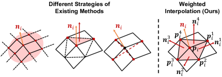
Figure 3: An illustration of different strategies of existing methods and the proposed surface normal fitting method (Eq. (4)). We mark the points, triangles, or lines that are leveraged to fit the surface normal in red for easy comparison. From left to right, method that uses excessive neighbor points [35], just a few points [30], a proper number of neighbor points while ignoring the information of query point [25], and our method that jointly considers a proper number of neighbor points and the query point.

Surface normal fitting. The surface normal fitting method in this work requires pixel-level accuracy and deals with the depth map that is dynamically optimized according to the backpropagation from fitting results. Existing solutions cannot be directly applied because they either use excessive neighbor points ($>4$) [35, 31] that reduces the precision of the fitted surface normal, or use just a few points [30] ($<4$) that brings ineffective backpropagation since the gradients affect a limit number of points on the depth map, or use a proper number of points ($=4$) while ignoring the information of the query point [25], as shown in Fig. 3. To solve these problems, we propose a weighted interpolation method to fit the surface normal that jointly considers the depth information of the query point and a proper number of neighbor points. As shown in Fig. 3, our method first computes normal vectors $\{\boldsymbol{n}_{i}^{k}|k=1,2,3,4\}$ of query’s adjacent triangles and then fit the normal $\boldsymbol{n}_{i}$ of the query point $\boldsymbol{p}_{i}$ by weighted interpolation of these vectors,

$${\footnotesize\begin{aligned} \boldsymbol{n}_{i}&=\sum_{k=1}^{4}\gamma^{k}_{i}\boldsymbol{n}^{k}_{i}=\sum_{k=1}^{4}\gamma^{k}_{i}\operatorname{Nor}[(\boldsymbol{p}^{k+1}_{i}-\boldsymbol{p}_{i})\times(\boldsymbol{p}_{i}^{k}-\boldsymbol{p}_{i})]^{\top},\\ \gamma^{k}_{i}&=\frac{|d^{k}_{i}|^{-1}}{\sum_{k=1}^{4}|d^{k}_{i}|^{-1}},~{}~{}~{}d^{k}_{i}=w^{k}_{i}+w_{i}^{k+1}-2w_{i},\\ \end{aligned}}$$ (4)

where $\boldsymbol{p}_{i}^{k}$ are adjacent points of $\boldsymbol{p}_{i}$, $k=1$ if $k+1>4$, ‘$\operatorname{Nor}$’ is the vector normalization operation, $w^{k}_{i}$ is the depth value of point $\boldsymbol{p}_{i}^{k}$. In this way, our method generates a high-precision normal map and backpropagates gradients to a proper number of points for the depth map optimization.

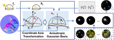
Figure 4: An illustration of building up the anisotropic reflectance model by Eq. (5). A group of ASG bases with various specular lobe’s widths ($r^{x}_{k}$ and $r^{y}_{k}$) [45] in the direction of tangent vector $\boldsymbol{x}_{i}$ and binormal vector $\boldsymbol{y}_{i}$ are multiplied by the corresponding spatially varying weight $c^{k}_{i}$ to compute $\rho^{s}_{ij}$.

4.2 Anisotropic Reflectance Modeling

We build up a more sophisticated and precise reflectance model to optimize the shape and light through anisotropic reflectance. As illustrated in Fig. 4, we represent the spatially varying anisotropic specularity as a weighted sum of Anisotropic Spherical Gaussian (ASG) [55] bases.

$$\begin{aligned} \rho_{ij}^{s}&=\sum_{k=1}^{N_{G}}c_{i}^{k}[e^{-r_{k}^{x}(\boldsymbol{h}_{j}\cdot\boldsymbol{x}_{i})^{2}-r_{k}^{y}(\boldsymbol{h}_{j}\cdot\boldsymbol{y}_{i})^{2}}],\\ \end{aligned}$$ (5)

where $k\in[1,2,...,N_{G}]$. $N_{G}$ is the number of the ASG bases empirically set as 12. $c_{i}^{k}$ is spatially varying weights that balance different ASG bases to model spatially varying specularity. $\boldsymbol{h}_{j}=\frac{\boldsymbol{V}_{d}+\boldsymbol{l}_{j}}{\|\boldsymbol{V}_{d}+\boldsymbol{l}_{j}\|}$ is the half-unit-vector between view direction $\boldsymbol{V}_{d}$ and light direction $\boldsymbol{l}_{j}$. $r_{k}^{x}$ and $r_{k}^{y}$ are the lobe’s width in the direction of $\boldsymbol{x}_{i}$ and $\boldsymbol{y}_{i}$, respectively. When $r_{k}^{x}=r_{k}^{y}$, ASG degrades to Isotropic Spherical Gaussian (ISG) bases. $\boldsymbol{x}_{i}$ and $\boldsymbol{y}_{i}$ are the tangent and binormal vectors, respectively, of the surface tangent plane at point $\boldsymbol{p}_{i}$. As shown in Fig. 4, $\boldsymbol{x}_{i}$ and $\boldsymbol{y}_{i}$ are calculated by:

$$\begin{aligned} \boldsymbol{x}_{i}=\boldsymbol{V}_{d}-(\boldsymbol{V}_{d}\cdot\boldsymbol{n}_{i})\boldsymbol{n}_{i},~{}~{}~{}\boldsymbol{y}_{i}=\boldsymbol{n}_{i}\times\boldsymbol{x}_{i}.\end{aligned}$$ (6)

The annealing strategy in [26] is adopted to control the number of activated ASG bases at different training stages, which helps avoid local optimum at the beginning.

4.3 Neural Inverse Rendering

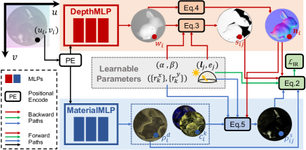
Figure 5: Framework overview of DANI-Net. DepthMLP takes the positional code as the input and outputs depth $w_{i}$. MaterialMLP takes the same positional code as the input and outputs $\rho_{i}^{d}$ and $c_{i}^{k}$. The shadow $s_{ij}$ is calculated based on Eq. (3). Spatially varying anisotropic specularity $\rho^{s}_{ij}$ is obtained through Eq. (5). Rendered images are generated through Eq. (2). The inverse rendering loss $\mathcal{L}_{\text{IR}}$ measures the rendering error between rendered images and observed images, and backpropagates to the light calibration and shape estimation through the differentiable shadow path (in red and green colors) and the anisotropic reflectance path (in blue and green colors).

As shown in Fig. 5, our neural inverse rendering framework integrates the differentiable shadow handling method and anisotropic reflectance model to two MLPs and several learnable parameters.

DepthMLP and MaterialMLP. To consider spatially-dependent information, we build up a neural depth field named DepthMLP and a neural material field named MaterialMLP, implemented by two MLPs. The DepthMLP estimates $w_{i}$ pixel-wisely; the MaterialMLP outputs $c^{k}_{i}$ and $\rho^{d}_{i}$ for spatially varying reflectance. We apply the same method [29] to encode the coordinate on the image plane.

Learnable parameters. As shown in Fig. 5, light conditions (i.e., $\boldsymbol{l}_{j}$, $e_{j}$), ASG lobe’s width parameters (i.e., $r^{x}_{k}$, $r^{y}_{k}$), and soft shadow parameters (i.e. $\alpha$ and $\beta$) are set as learnable parameters. We initialize $\boldsymbol{l}_{j}$ and $e_{j}$ using outputs of a pre-trained light calibration model, i.e., we apply the CNN structures in [26] and train on the Blobby and Sculpture dataset [9]. We set the scope of $r^{x}_{k}$ and $r^{y}_{k}$ in $[10^{0},10^{3}]$ and initialize $r^{x}_{k}=r^{y}_{k}=10^{\frac{(\log 300-\log 10)(k-1)}{N_{G}-1}+\log 10}$ (i.e., uniformly sampled ${N_{G}}$ values from $[10,300]$ in the log space) to force an isotropic reflectance model and consider different sharpness at the beginning, which enables a smooth transition to the anisotropic reflectance. $\alpha$ and $\beta$ are empirically initialized to 400 and 3.

A rendered image is calculated through Eq. (2) using the outputs from the two MLPs and the learnable parameters. The inverse rendering $\ell_{1}$ metric error $\mathcal{L}_{\text{IR}}$ between the rendered images and the observed images given by Eq. (7) passes through the differentiable paths to jointly update weights of MLPs and learnable parameters,

$$\footnotesize\mathcal{L}_{\text{IR}}=\frac{1}{\text{\#}\mathbb{P}\times f}\sum_{i=1}^{\text{\#}\mathbb{P}}\sum_{j=1}^{f}{|\bar{m}_{ij}-e_{j}s_{ij}(\rho^{d}_{i}+\rho^{s}_{ij})\max(\boldsymbol{n}_{i}^{\top}\boldsymbol{l}_{j},0)|}.$$ (7)

Table 2: Quantitative comparison in terms of MAE of surface normal on DiLiGenT benchmark dataset [40]. Bold numbers and underlined numbers indicate the best and the second-best results among UPS methods, respectively.

Method	Ball	Bear	Buddha	Cat	Cow	Goblet	Harvest	Pot1	Pot2	Reading	AVG
LS [48]	4.10	8.39	14.92	8.41	25.60	18.50	30.62	8.89	14.65	19.80	15.39
TM18 [43]	1.47	5.79	10.36	5.44	6.32	11.47	22.59	6.09	7.76	11.03	8.83
LL22 [25]	2.43	3.64	8.04	4.86	4.72	6.68	14.90	5.99	4.97	8.75	6.50
PF14[34]	4.77	9.07	14.92	9.54	19.53	29.93	29.21	9.51	15.90	24.18	16.66
CH19 [8]	2.77	6.89	8.97	8.06	8.48	11.91	17.43	8.14	7.50	14.90	9.51
CW20 [10]	2.50	5.60	8.60	7.90	7.80	9.60	16.20	7.20	7.10	14.90	8.71
SCPS-NIR [26]	1.24	3.82	9.28	4.72	5.53	7.12	14.96	6.73	6.50	10.54	7.05
DANI-Net w/o $s$	1.71	3.95	8.71	4.95	4.95	6.80	16.00	7.04	5.27	9.32	6.87
DANI-Net w [25]	1.64	4.03	9.16	5.27	5.22	6.98	16.43	6.85	5.52	9.53	7.06
DANI-Net	1.65	4.11	8.69	4.73	5.52	6.96	13.99	6.41	5.29	8.08	6.54

4.4 Optimizing DANI-Net

In addition to the inverse rendering loss function, the proposed DANI-Net is optimized by the silhouette loss function $\mathcal{L}_{\text{Si}}$ and the smooth loss function. The silhouette loss function $\mathcal{L}_{\text{Si}}$ is similar to those in [15, 10, 26] by calculating the cosine similarity between estimated and fitted silhouette’s normal. The fitted surface normals at the silhouette alleviate the GBR ambiguity because the GBR transformation on these surface normals equals an identity matrix. Our smoothness loss function focuses on the diffuse reflectance map $R^{d}$, the normal map $\boldsymbol{N}$, and the depth map $W$, which follows the similar implementation in [26, 25],

$${\footnotesize\begin{aligned} \mathcal{L}_{\text{smooth}}=&\lambda\mathcal{L}_{R^{d}}+\lambda\mathcal{L}_{W}+\lambda_{N}\mathcal{L}_{N}\\ =&\lambda\frac{1}{\#\mathbb{P}}\sum_{i=1}^{\#\mathbb{P}}|\frac{\partial R^{d}}{\partial u}+\frac{\partial R^{d}}{\partial v}|+\lambda\frac{1}{\#\mathbb{P}}\sum_{i=1}^{\#\mathbb{P}}|\frac{\partial W}{\partial u}+\frac{\partial W}{\partial v}|\\ +&\lambda_{N}\frac{1}{\#\mathbb{P}}\sum_{i=1}^{\#\mathbb{P}}|\frac{\partial\boldsymbol{N}}{\partial u}+\frac{\partial\boldsymbol{N}}{\partial v}|.\end{aligned}}$$ (8)

We train the DANI-Net in three stages for fast convergence. The loss function in three stages is as follows,

$$\begin{aligned} \mathcal{L}_{\text{stage1}}=&\mathcal{L}_{\text{IR}}+\lambda_{\text{Si}}\mathcal{L}_{\text{Si}}+\mathcal{L}_{\text{smooth}},\\ \mathcal{L}_{\text{stage2}}=&\mathcal{L}_{\text{IR}}+\lambda_{\text{Si}}\mathcal{L}_{\text{Si}}+\lambda\mathcal{L}_{N},\\ \mathcal{L}_{\text{stage3}}=&\mathcal{L}_{\text{IR}}+\lambda_{\text{Si}}\mathcal{L}_{\text{Si}},\end{aligned}$$ (9)

where $\lambda=0.01$, $\lambda_{N}=0.02$, and $\lambda_{\text{Si}}=0.01$. Three stages take 500, 1000, and 500 epochs, respectively. We also apply a progressive training schema with the learning rate decaying in a cosine annealing manner. During training, we use Adam as the optimizer with a learning rate $\alpha_{l}=0.001$ decaying to $0.0001$ for 2000 epochs.

5 Experiments

Evaluation Metrics. To evaluate the accuracy of the predicted light directions and surface normal, we adopt mean angle error (MAE) in degree. To evaluate the accuracy of recovered light intensity free from the reflectance-light ambiguity, we use the scale-invariant relative error [8], $E_{\text{int}}=\frac{1}{f}\sum_{j=1}^{f}\left(\frac{\left|\eta e_{j}-\tilde{e}_{j}\right|}{\tilde{e}_{j}}\right)$, where $\tilde{e}_{j}$ is the ground truth light intensity, $e_{j}$ is the estimated light intensity, and $\eta$ is calculated through solving $\mathop{\arg\min}_{\eta}\sum_{j=1}^{f}\left(\eta e_{j}-\tilde{e}_{j}\right)^{2}$ by least squares.

Datasets. We evaluate our method on DiLiGenT [40] and DiLiGenT$10^{2}$ benchmark dataset [36].

5.1 Performance on DiLiGenT [40]

We compare with six state-of-the-art photometric stereo methods on DiLiGenT dataset [40], including two unsupervised calibrated PS methods (TM18 [43] and LL22 [25]), two supervised UPS methods (CH19 [8] and CW20 [10]), and an unsupervised UPS method (SCPS-NIR [26]). We also include two baseline methods for PS (LS [48]) and UPS (PF14 [34]).

Surface normal estimation. Table 2 shows that DANI-Net outperforms other UPS methods and achieves comparable performance as the state-of-the-art calibrated PS method LL22 [25]. For Reading and Harvest that contain substantial cast shadow, DANI-Net achieves a superior performance advantage over the other methods because our differentiable handling method simultaneously optimizes the shadow map with other unknowns, ensuring full utilization of shadow cues. For Cow and Goblet with a more prominent anisotropic reflectance as compared to other objects, DANI-Net also achieves the best performance, validating the effectiveness of our anisotropic material model.

Table 3: Quantitative comparison in terms of MAE of light direction and scale-invariant error of intensity on DiLiGenT benchmark dataset [40]. Bold numbers and underlined numbers indicate the best and the second-best results, respectively.

Model	Ball		Bear		Buddha		Cat		Cow		Goblet		Harvest		Pot1		Pot2		Reading		AVG
	dir.	int.	dir.	int.	dir.	int.	dir.	int.	dir.	int.	dir.	int.	dir.	int.	dir.	int.	dir.	int.	dir.	int.	dir.	int.
PF14 [34]	4.90	0.036	5.24	0.098	9.76	0.053	5.31	0.059	16.34	0.074	33.22	0.223	24.99	0.156	2.43	0.017	13.52	0.044	21.77	0.122	13.75	0.088
CH19 [8]	3.27	0.039	3.47	0.061	4.34	0.048	4.08	0.095	4.52	0.073	10.36	0.067	6.32	0.082	5.44	0.058	2.87	0.048	4.50	0.105	4.92	0.068
CW20 [10]	1.75	0.027	2.44	0.101	2.86	0.032	4.58	0.075	3.15	0.031	2.98	0.042	5.74	0.065	1.41	0.039	2.81	0.059	5.47	0.048	3.32	0.052
SCPS-NIR [26]	1.43	0.019	1.56	0.019	4.22	0.021	4.41	0.032	4.94	0.062	2.26	0.042	6.41	0.023	3.46	0.030	4.19	0.082	7.34	0.035	4.02	0.037
DANI-Net w/o $s$	1.25	0.020	2.08	0.026	2.50	0.021	3.09	0.027	2.12	0.059	2.89	0.047	5.27	0.026	4.23	0.031	2.76	0.086	5.45	0.026	3.16	0.037
DANI-Net w[25]	1.24	0.020	1.69	0.024	3.07	0.021	3.28	0.026	2.41	0.058	3.01	0.043	6.47	0.030	4.50	0.029	3.30	0.084	5.37	0.025	3.43	0.036
DANI-Net	1.23	0.020	3.71	0.022	2.63	0.025	3.32	0.029	4.19	0.055	1.65	0.044	6.34	0.026	4.17	0.029	3.42	0.079	3.28	0.028	3.39	0.036

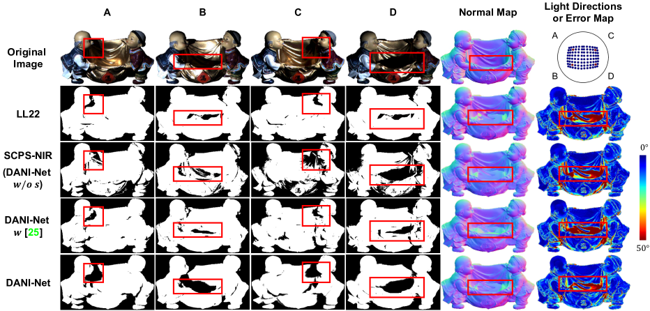
Figure 6: A visual quality comparison on shadow maps (cast and attached shadow) and surface normal among LL22 [25], SCPS-NIR [26], DANI-Net w/o s, DANI-Net w [25], and DANI-Net on Harvest from DiLiGenT [40]. The four left columns are images/shadow maps under four light directions, labeled by ABCD, indicated by red dots shown in the light direction figure on the top right. The two right columns are the ground truth or estimated normal maps and error maps. Red boxes highlight prominent regions for easy comparison.

Light calibration. As shown in Table 3, our method achieves the best light intensity and the second-best light direction calibration results. Interestingly, although CW20 [10] achieves better light direction calibration results than DANI-Net, it achieves a less comparable performance of surface normal estimation. The reason could be that CW20 [10] and other two-stage methods suffer from the accumulating error brought by the light calibration stage.

Differentiable shadow handling validation. To validate the effectiveness of our differentiable shadow handling method, we compare it with ‘DANI-Net w/o $s$’ and ‘DANI-Net w [25]’, which are two alternatives of DANI-Net without differentiable shadow handling. As compared with DANI-Net, the only difference of the two alternatives are shadow handling method (i.e., DANI-Net w/o $s$ uses the same fixed shadow map in SCPS-NIR [26]; DANI-Net w[25] uses same shadow handling method in [25]). As can be observed in Table 2 and Table 3, the performance of DANI-Net w/o $s$ and DANI-Net w [25] drops on surface normal estimation (the average MAE increases $0.33^{\circ}$ and $0.52^{\circ}$, respectively), while remains similar on light calibration compared with DANI-Net. However, as shown in Fig. 6, DANI-Net generates much more realistic and smooth shadow maps than its alternatives. This is because the shadow maps’ calculation in [26, 25] suffers from certain limitations. For [26], shadow maps are calculated based on pixel intensities rather than depth and light which can be affected by surface points with dark color; for [25], shadow maps are explicitly calculated based on depth and light but are sensitive to the accumulating error in the depth map at a specific epoch. In contrast, DANI-Net overcomes these limitations by explicitly calculating shadow maps based on iteratively optimized depth and light, free from impact of surface points with dark color and accumulating errors in the depth map, leading to high-quality shadow maps.

Table 4: Quantitative comparison in terms of MAE of surface normal on Ball and Bunny with 10 different materials from DiLiGenT$10^{2}$ benchmark dataset [36]. Bold numbers and underlined numbers indicate the best and the second-best results, respectively.

c—c—cccccc—ccc—c—c Object Method Isotropic Group Anisotropic Chall. Group AVG
Pom Pp Nylon Pvc Abs Bakelite Al Cu Steel Acrylic
Ball CNN-PS [20] 5.10 6.40 4.20 4.50 6.90 7.30 15.90 14.10 16.40 19.10 9.99
CH19 [8] 4.40 2.10 4.60 4.50 3.20 4.30 15.30 19.70 21.90 42.40 12.24
CW20 [10] 10.10 3.01 9.84 7.13 5.64 4.94 21.49 24.01 27.04 37.92 15.11
SCPS-NIR [26] 3.07 2.30 9.28 1.40 5.29 5.23 20.27 26.82 27.11 57.75 15.85
DANI-Net 2.04 3.15 7.06 4.14 2.87 6.07 3.94 11.75 8.03 34.14 8.32
Bunny CNN-PS [20] 24.30 11.40 27.20 7.80 20.80 9.10 12.40 7.70 11.60 14.40 14.67
CH19 [8] 29.00 18.00 29.00 17.00 28.00 18.00 28.00 16.00 23.00 33.00 23.90
CW20 [10] 19.88 11.64 22.36 9.49 18.63 12.55 18.03 12.54 17.85 28.54 17.15
SCPS-NIR [26] 22.81 9.49 26.76 7.44 19.39 9.82 21.52 8.13 18.55 26.20 17.01
DANI-Net 19.55 7.57 23.82 6.59 16.49 7.81 10.36 6.76 6.16 21.89 12.70

Table 5: Quantitative comparison in terms of MAE of surface normal on the ‘anisotropic group’ of DiLiGenT$10^{2}$ benchmark dataset [36] with 10 materials. Bold numbers and underlined numbers indicate the best and the second-best results, respectively.

Material	Method	Ball	Golf	Spike	Nut	Square	Pentagon	Hexagon	Propeller	Turbine	Bunny	AVG
Al	CNN-PS [19]	15.90	11.60	14.30	16.10	13.40	14.60	18.30	16.40	25.20	12.40	15.82
	SCPS-NIR [26]	20.27	15.20	25.66	22.60	18.37	24.25	32.38	33.14	31.20	21.52	24.46
	DANI-Net w/o ASG	17.51	10.01	20.45	17.57	14.22	14.78	14.81	28.88	33.61	12.34	18.42
	DANI-Net	3.94	7.23	10.59	14.50	11.56	14.04	14.25	37.09	32.33	10.36	15.59
Cu	CNN-PS [20]	14.10	9.20	8.30	13.00	4.90	12.80	10.40	9.60	22.40	7.70	11.24
	SCPS-NIR [26]	26.82	9.86	8.92	25.71	27.16	39.35	11.89	14.72	28.96	8.13	20.15
	DANI-Net w/o ASG	20.03	7.07	7.42	12.03	6.75	22.53	7.38	9.75	24.90	7.40	12.53
	DANI-Net	11.75	6.44	6.08	10.46	6.43	15.89	6.66	10.15	23.79	6.76	10.44
Steel	CNN-PS [20]	16.40	13.40	16.10	13.90	7.90	15.50	16.90	9.80	21.50	11.60	14.30
	SCPS-NIR [26]	27.11	20.54	29.22	16.07	33.37	36.84	27.23	27.69	34.15	18.55	27.08
	DANI-Net w/o ASG	20.16	8.43	22.89	11.45	17.83	13.60	13.47	20.88	24.71	8.92	16.23
	DANI-Net	8.03	7.50	11.85	9.95	12.95	15.24	11.29	21.63	32.66	6.16	13.73

5.2 Performance on DiLiGenT$10^{2}$ [36]

To conduct an in-depth analysis of DANI-Net regarding its generalization ability on different light conditions and imaging setups, we test DANI-Net on the challenging DiLiGenT$10^{2}$ benchmark dataset [36]. As the supervised calibrated PS method CNN-PS [19] achieves the best performance on DiLiGenT$10^{2}$ [36] according to [36], we also compare with it in this section.

Surface normal estimation. To evaluate the performance of DANI-Net on a variety of materials, we test it on 10 different materials with two typical shapes of simple Ball and general Bunny. In additional to the state-of-the-art supervised PS method CNN-PS [19], we also compare with three state-of-the-art UPS methods CH19 [8], CW20 [10], and SCPS-NIR [26]. As can be observed in Table 5.1, DANI-Net achieves the best performance for surface normal estimation and even outperforms the supervised PS method CNN-PS [19], especially for anisotropic materials of Steel, Cu, and Al. It owes to our anisotropic reflectance modeling and differentiable shadow handling method. However, DANI-Net is less competitive on Acrylic material with a translucent effect due to the absence of explicit modeling of translucent BRDFs.

Anisotropic reflectance modeling validation. To further testify the effectiveness of the anisotropic reflectance model in DANI-Net, we conduct experiments on the ‘anisotropic group’ of DiLiGenT$10^{2}$ benchmark dataset [40] with 10 different shapes. In addition to the state-of-the-art methods, CNN-PS [19] (supervised and calibrated) and SCPS-NIR [26] (unsupervised and uncalibrated), we also compare with ‘DANI-Net w/o ASG’, which is the alternative of DANI-Net with isotropic reflectance modeling. That is, we apply ISG bases instead of ASG bases by setting $r_{k}^{x}=r^{y}_{k}$ in Eq. (5) during training. As can be observed from Table 5, DANI-Net outperforms CNN-PS [19] and SCPS-NIR [26] for all cases except for shapes of Propeller and Turbine, where the averaged MAE of these two shapes over three materials (i.e., Al, Cu, and Steel) is $26.27^{\circ}$. This is because DANI-Net takes a poor initialization of light from [26] on these two shapes. Even so, DANI-Net achieves the best numbers in average across different shapes. Table 5 also shows an observable performance degradation of ‘DANI-Net w/o ASG’ due to its isotropic reflectance modeling, which indicates the effectiveness of using the anisotropic reflectance model.

6 Conclusion

This paper proposes DANI-Net to address UPS in an unsupervised manner. Thanks to shadow handling and anisotropic reflectance modeling, DANI-Net can address more general objects with complicated shadows and materials. This paper also presents solutions for shadow calculation and surface normal fitting for differentiable shadow handling. Our unsupervised training manner and anisotropic reflectance modeling are beneficial for generalizing DANI-Net to data from different sources.

Limitations and future work. Although our method produces promising results for light conditions and surfaces normal estimation on multiple real-world datasets, it has several limitations. First, DANI-Net cannot handle objects with strong inter-reflections or translucent materials. Second, the image’s noise caused by overexposure or underexposure will degrade the performance of the proposed DANI-Net and other inverse rendering methods. Third, we have a longer testing time compared to [26] (i.e., 34 minutes for DANI-Net vs. 14 minutes for [26] in average per objects in DiLiGenT [40]). Given DANI-Net’s performance on anisotropic materials, building up a more sophisticated reflectance model to consider the translucent effect and inter-reflection is worth exploring in the future.

Acknowledgments. This work is supported by National Natural Science Foundation of China under Grant No. 61925603, 62136001, 62088102.

Supplementary Material

In this supplementary material,

1. we provide more details about the network architectures in Sec. A (footnote 5 in the main paper);

2. we show the complete qualitative comparison of 10 objects from DiLiGenT [40] dataset between DANI-Net and other state-of-the-art methods [10, 25, 26] in Sec. B (footnote 9 in the main paper); we also conduct additional experiments to validate the effectiveness of our normal fitting method and visualize the generated svBRDF in this section (footnote 3 in the main paper);

3. we conduct more ablation studies about our three-stage training schema and silhouette loss in Sec. C (footnote 7 in the main paper);

4. we show the complete quantitative comparison of 100 objects (i.e., 10 shapes multiplying 10 different materials) from DiLiGenT$10^{2}$ dataset [36] and visualization of the fitted material on 2 selected shapes (i.e., Ball, Bunny) with 3 anisotropic materials (i.e., Al, Cu, and Steel) in Sec. D (footnote 11 in the main paper); we also analyze the effects of different initialization methods in this section (footnote 12 in the main paper);

5. we show the qualitative and quantitative results on 3 objects from Apple & Gourd dataset [2] and 6 objects from Light Stage Data Gallery dataset [6] in Sec. E (footnote 8 in the main paper).

The code is available at https://github.com/LMozart/CVPR2023-DANI-Net.

Appendix A Implementation Details

Positional encoding. We apply the same positional encoding module in NeRF [29] given the following equation,

$$E(p)=\left(\sin\left(2^{0}\pi p\right),\cos\left(2^{0}\pi p\right),\cdots,\sin\left(2^{L-1}\pi p\right),\cos\left(2^{L-1}\pi p\right)\right),$$ (10)

where $L$ is the dimension of the positional code, $p$ is 2D coordinate $(u_{i},v_{i})$ in the image plane for DepthMLP and MaterialMLP. We compute the positional code $E(p)$ for each dimension and concatenate these codes to get our positional code.

Network structure. We show the details of the DepthMLP and MaterialMLP in Fig. 7. We use the same pre-trained light model as [26] for light initialization. More details of the pre-trained light model can be found in the supplementary materials of SCPS-NIR [26].

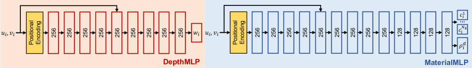
Figure 7: Network structures of DepthMLP and MaterialMLP.

Appendix B Additional Results on DiLiGenT Dataset [40]

Qualitative results on DiLiGenT dataset [40]. From Fig. 8 to Fig. 11 we show the normal map, error map, and light map of 10 objects from DiLiGenT Dataset [40] predicted by DANI-Net and its alternatives (i.e., DANI-Net w [25] and DANI-Net w/o $s$). We further compare DANI-Net with recent UPS methods [26, 10] and state-of-the-art unsupervised PS methods [25]. The results illustrate the effectiveness of the differentiable shadow handling and anisotropic material modeling method in DANI-Net.

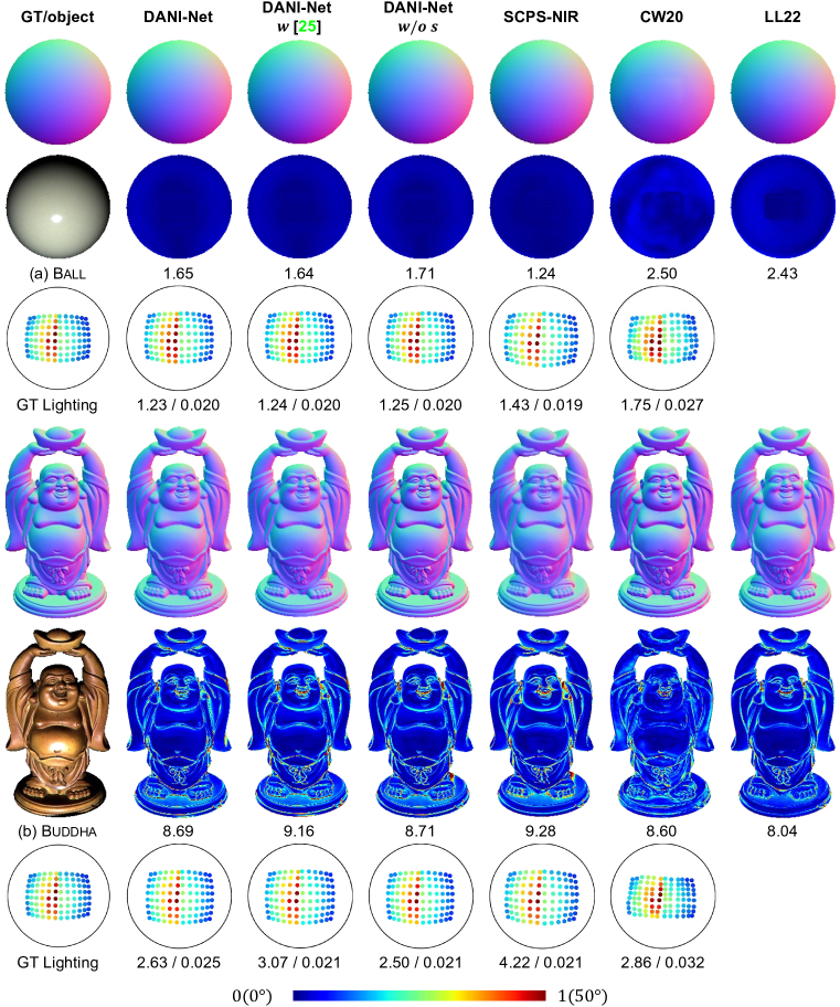
Figure 8: The visual quality comparison among DANI-Net, DANI-Net w [25], DANI-Net w/o $s$, SCPS-NIR [26], CW20 [10], and LL22 [25] on Ball and Buddha from DiLiGenT [40] in terms of normal map (row 1,4), error map (row 2, 5), and light map (row 3, 6). Numbers indicate the MAE (for surface normal or light directions) or scale-invariant relative error (for light intensity).

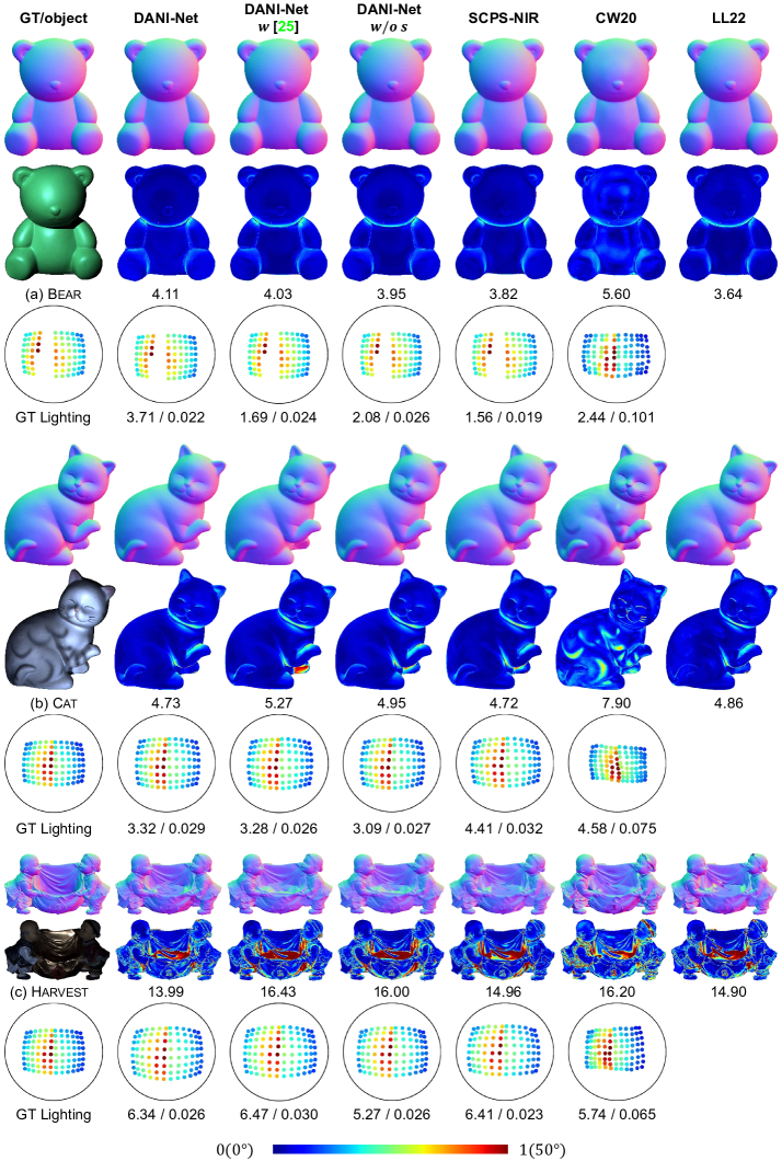
Figure 9: The visual quality comparison among DANI-Net, DANI-Net w [25], DANI-Net w/o $s$, SCPS-NIR [26], CW20 [10], and LL22 [25] on Bear, Cat, and Harvest from DiLiGenT [40] in terms of normal map (row 1, 4, 7), error map (row 2, 5, 8), and light map (row 3, 6, 9). Numbers indicate the MAE (for surface normal or light directions) or scale-invariant relative error (for light intensity).

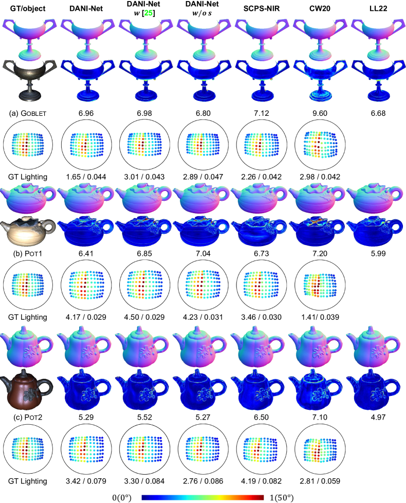
Figure 10: The visual quality comparison among DANI-Net, DANI-Net w [25], DANI-Net w/o $s$, SCPS-NIR [26], CW20 [10], and LL22 [25] on Goblet, Pot1, and Pot2 from DiLiGenT [40] in terms of normal map (row 1, 4, 7), error map (row 2, 5, 8), and light map (row 3, 6, 9). Numbers indicate the MAE (for surface normal or light directions) or scale-invariant relative error (for light intensity).

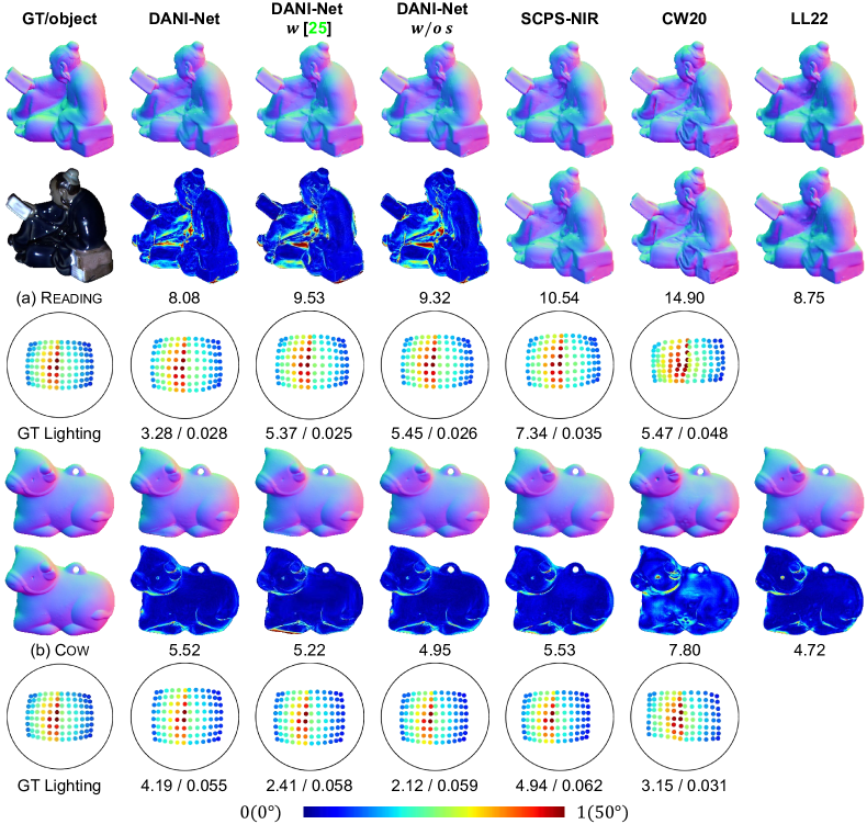
Figure 11: The visual quality comparison among DANI-Net, DANI-Net w [25], DANI-Net w/o $s$, SCPS-NIR [26], CW20 [10], and LL22 [25] on Reading and Cow from DiLiGenT [40] in terms of normal map (row 1,4), error map (row 2, 5), and light map (row 3, 6). Numbers indicate the MAE (for surface normal or light directions) or scale-invariant relative error (for light intensity).

Validation of weighted interpolation. To validate the effectiveness of our weighted interpolation for normal fitting, we compare DANI-Net with ‘DANI-Net w sobel’ (i.e., Sobel operator), ‘DANI-Net w cross’ (i.e., method in [25]), and ‘DANI-Net w triangle’ (i.e., method in [31]). Those alternatives are only different in the normal fitting method. As shown in Table 6, DANI-Net outperforms all alternatives on average, especially on objects like Harvest with a complicated shape. We observe a similar performance between ‘DANI-Net w sobel’ and ‘DANI-Net w cross’, whose average MAE on normal estimation increase $0.15^{\circ}$ and $0.09^{\circ}$, respectively since they either ignore query point’s information or using excessive neighbor points. The average MAE of ‘DANI-Net w triangle’ increase about $0.39^{\circ}$ due to its ineffectiveness in backpropagation (i.e., limit points affected by the gradients).

Table 6: Quantitative comparison in terms of MAE of surface normal on DiLiGenT benchmark dataset [40] for different normal fitting methods. Bold numbers indicates the best results.

Method	Ball	Bear	Buddha	Cat	Cow	Goblet	Harvest	Pot1	Pot2	Reading	AVG
DANI-Net w triangle	2.33	4.27	9.19	4.87	5.65	7.44	15.22	6.61	5.69	8.01	6.93
DANI-Net w sobel	1.89	3.97	9.05	4.71	5.31	7.27	14.85	6.72	5.42	7.68	6.69
DANI-Net w cross	1.88	3.98	9.08	4.70	5.36	6.67	14.93	6.63	5.43	7.68	6.63
DANI-Net	1.65	4.11	8.69	4.73	5.52	6.96	13.99	6.41	5.29	8.08	6.54

Validation of svBRDF. To validate the spatially varying BRDF (svBRDF) generated by DANI-Net, we visualize the BRDF spheres at different points of Harvest, Reading, and Pot1 in Fig. 12. The spheres show polychrome appearances with different roughness, demonstrating the visually pleasant svBRDF generated by DANI-Net.

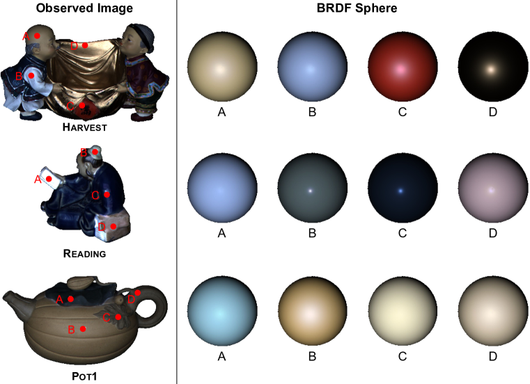
Figure 12: Visualization of the estimated svBRDF on Harvest, Reading, and Pot1 from DiLiGenT dataset [40]. On each object, we select four points (red dots on the first column’s images, labeled ABCD) at different positions with different materials to showcase the predicted svBRDF spheres. The overall intensity of the observed images and BRDF spheres is scaled for better visualization.

Appendix C Additional Ablation Studies

C.1 Three-stage Training Schema

The smoothness terms incorporated in the three-stage training schema (i.e., $\mathcal{L}_{R^{d}},\mathcal{L}_{W},$ and $\mathcal{L}_{N}$) facilitate DANI-Net’s convergence at an early stage (stage 1); while they are gradually dropped in the subsequent stage (stage 2, 3) to avoid over-smooth results. To validate the effectiveness of the three-stage training schema, we compare DANI-Net with: 1) ‘DANI-Net w $\mathcal{L}_{N}$’ that keeps $\mathcal{L}_{N}$ till the training complete; 2) ‘DANI-Net w/o $\mathcal{L}_{R^{d}}$’ that drops material smoothness term (i.e., $\mathcal{L}_{R^{d}}$) at the beginning on DiLiGenT dataset [40]; 3) ‘DANI-Net w/o $\mathcal{L}_{N}+\mathcal{L}_{W}$’ that drops geometry smoothness terms (i.e., $\mathcal{L}_{N}$ and $\mathcal{L}_{W}$) at the beginning. As shown in Table 7, the average MAE of normal estimation on 10 objects increases $0.22^{\circ}$, $0.28^{\circ}$, and $0.10^{\circ}$ for ‘DANI-Net w $\mathcal{L}_{N}$’, ‘DANI-Net w/o $\mathcal{L}_{R^{d}}$’, and ‘DANI-Net w/o $\mathcal{L}_{N}+\mathcal{L}_{W}$’, respectively, indicating the necessity of the three-stage training schema.

Table 7: Quantitative comparison in terms of MAE of surface normal on DiLiGenT benchmark dataset [40] for different alternatives on three-stage training schema. Bold numbers indicates the best results.

Method	Ball	Bear	Buddha	Cat	Cow	Goblet	Harvest	Pot1	Pot2	Reading	AVG
DANI-Net w $\mathcal{L}_{N}$	1.57	4.10	9.76	4.99	5.16	6.96	14.41	7.28	5.88	7.47	6.76
DANI-Net w/o $\mathcal{L}_{R^{d}}$	1.47	4.05	8.79	5.15	5.69	6.97	14.28	7.13	5.24	9.43	6.82
DANI-Net w/o $\mathcal{L}_{N}+\mathcal{L}_{W}$	1.44	4.28	8.19	4.98	5.92	6.88	15.29	6.08	5.28	8.06	6.64
DANI-Net	1.65	4.11	8.69	4.73	5.52	6.96	13.99	6.41	5.29	8.08	6.54

C.2 Silhouette Normal

Although the fitted silhouette normal is only reliable at the occluding boundaries, the silhouette loss $\mathcal{L}_{\text{Si}}$ is crucial in alleviating GBR ambiguity that facilitates DANI-Net’s convergence and prevents it from falling into the local optimum. We compare DANI-Net with ‘DANI-Net w/o $\mathcal{L}_{\text{Si}}$’ (or $\mathcal{L}_{\text{Si}}$) that drops $\mathcal{L}_{\text{Si}}$ at the beginning (or at stage 3) on DiLiGenT dataset [40]. As shown in Table 8, the average MAE of normal estimation on 10 objects increases $0.52^{\circ}$ (or $0.14^{\circ}$), indicating the necessity of silhouette loss.

For objects in Light Stage Data Gallery [6] and DiLiGenT $10^{2}$ [36] with non-occluding silhouette, DANI-Net uses silhouette loss in a more flexible way. That is, we either drop the silhouette loss at stage 3 (Knight Kneeling, Knight Fighting, and Knight Standing from Light Stage Data Gallery [6]), or roughly estimate the silhouette’s normal instead of pre-computing it through silhouette’s perpendicular vectors (Bunny, Hexagon, Nut, Pentagon, Propeller, Square, and Turbine from DiLiGenT $10^{2}$ [36]). To clarify the necessity of this strategy, we visualize the estimated normal map of DANI-Net and ‘DANI-Net w $\mathcal{L}_{\text{Si}}$’ that keeps $\mathcal{L}_{\text{Si}}$ in all stages on Knight Fighting with partially non-occluding silhouettes on the sword (the top row of Fig. 13), and Nut Pp with predominantly non-occluding silhouettes on its base (the bottom row of Fig. 13). It can be observed that keeping $\mathcal{L}_{\text{Si}}$ in all stages does not significantly affect the normal estimation results for objects with partially occluding silhouettes like Knight Fighting, but it does harm the performance for objects with predominantly non-occluding silhouettes (MAE on normal estimation increases $1.16^{\circ}$ on Nut Pp). This validates the effectiveness of our flexible strategy using $\mathcal{L}_{\text{Si}}$ on objects with non-occluding silhouettes.

Table 8: Quantitative comparison in terms of MAE of surface normal on DiLiGenT benchmark dataset [40] for different alternatives on silhouette loss. Bold numbers indicates the best results.

Method	Ball	Bear	Buddha	Cat	Cow	Goblet	Harvest	Pot1	Pot2	Reading	AVG
DANI-Net w/o $\mathcal{L}_{\text{Si}}$	1.68	4.22	9.44	5.30	5.79	8.12	14.18	7.43	5.53	8.89	7.06
DANI-Net w/o $\mathcal{L}_{\text{Si}}$-3	1.81	4.07	8.72	5.15	5.69	7.10	13.77	6.95	5.26	8.30	6.68
DANI-Net	1.65	4.11	8.69	4.73	5.52	6.96	13.99	6.41	5.29	8.08	6.54

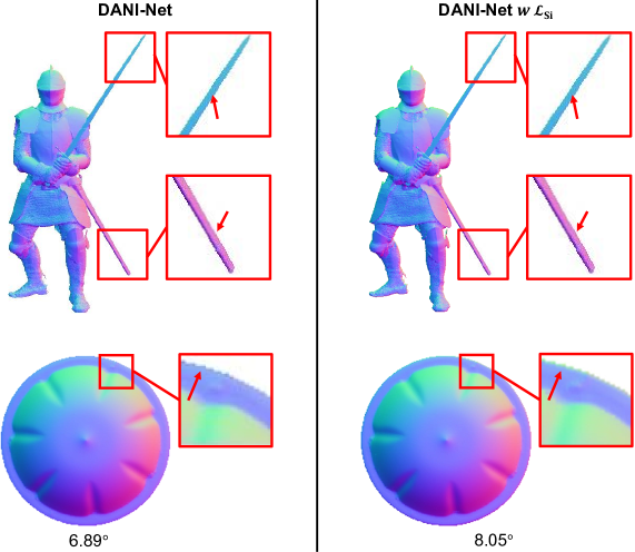
Figure 13: Visualization of the estimated normal map on Knight Fighting (top), and Nut Pom (bottom) from Light Stage Data Gallery [6] and DiLiGenT$10^{2}$ [36]. Sub-figures in the left (or right) column are normal maps estimated by DANI-Net (or ‘DANI-Net w $\mathcal{L}_{\text{Si}}$’) Red boxes highlight prominent regions for easy comparison. Red arrows point to the silhouette of objects. Numbers at the bottom indicate the MAE of normal estimation.

Appendix D Additional Results on DiLiGenT$10^{2}$ Dataset [36]

Quantitative results of normal estimation. Fig. 14 presents the comprehensive normal estimation results compared with CW20 [10], SCPS-NIR [26], and CNN-PS [19]. While DANI-Net outperforms current methods on Ball and Bunny or anisotropic group (i.e., Al, Cu, and Steel), the average MAE of DANI-Net on 100 objects’ normal estimation is slightly higher than CNN-PS (still lower than current UPS methods). Particularly, we find that DANI-Net is not competitive on objects of Nylon and Acrylic, and objects like Turbine and Propeller with complicated shapes in the ‘anisotropic group’.

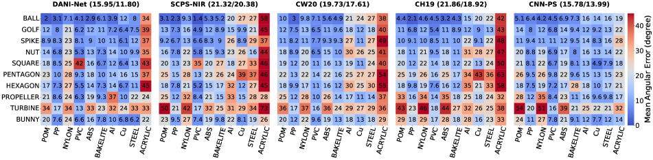
Figure 14: Normal estimation results on DiLiGenT$10^{2}$ Dataset [36] visualized by Shape-material error matrix [36]. Numbers in the bracket indicate each method’s mean/median MAE for normal estimation.

Quantitative results of light calibration. Fig. 15 and Fig. 16 present the light calibration results, compared with CW20 [10], SCPS [8], and SCPS-NIR [26]. As can be observed in those figures, DANI-Net reaches the second-best performance on light direction calibration and the best on light intensity calibration. By cross-comparing the results of normal estimation, we find that the cases with high normal estimation MAE also result in particularly high MAE in light calibration.

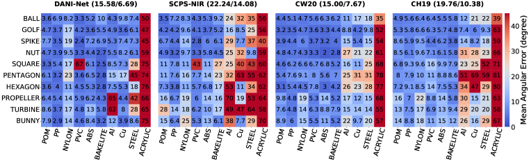
Figure 15: Light direction calibration results on DiLiGenT$10^{2}$ Dataset [36] visualized by Shape-material error matrix [36]. Numbers in the bracket indicate each method’s mean/median MAE for light direction calibration.

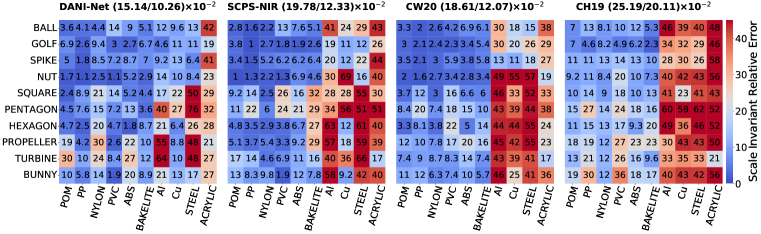
Figure 16: Light intensity calibration results on DiLiGenT$10^{2}$ Dataset [36] visualized by Shape-material error matrix [36]. The number in the matrix is scaled for visualization. Numbers in the bracket indicate each method’s mean/median scale invariant relative error for light intensity calibration.

Analysis on light initialization. We first conjecture that inadequate light initialization is the main cause of inaccurate normal estimation. To validate that, we showcase the initial light’s (calibrated by the pre-trained light model [26]) MAE in Fig. 17.

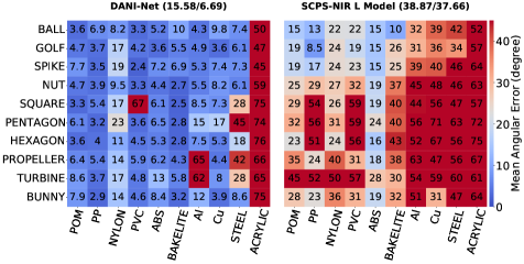
Figure 17: Comparison between DANI-Net and the pre-trained light model of SCPS-NIR [26] on light calibration. Numbers in the bracket indicate each method’s mean/median MAE for light direction calibration.

The results validate our conjecture, i.e., the initial lights deviate significantly from the ground truth in the aforementioned cases. Therefore, initializing the light more accurately will be a reasonable strategy (e.g., light calibrated by GCNet [10]). We compare DANI-Net with ‘DANI-Net+GCNet’, with the latter differing only in its light initialized by GCNet. As shown in Fig. 18, the average MAE of normal estimation (or light calibration) of ‘DANI-Net+GCNet’ decreases $0.77^{\circ}$ (or $3.06^{\circ}$). Particularly, we observe a compelling enhancement for objects with complicated shapes (i.e., Propeller, Turbine), but a marginal improvement for objects made of Nylon and Acrylic. While objects made of Acrylic still have inaccurate light initialization leading to unsatisfactory light calibration and normal estimation, the results obtained for objects made of Nylon contradict our earlier conjecture. We further assume that the materials’ exceptional properties may be the primary cause of the subpar performance.

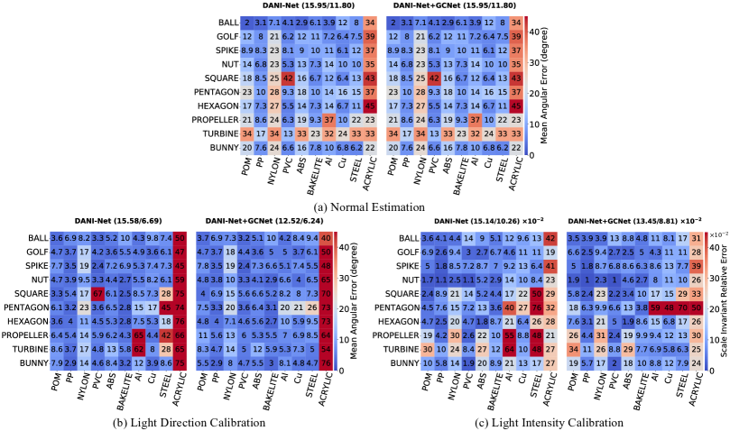
Figure 18: Comparison between DANI-Net and DANI-Net+GCNet on normal estimation and light calibration. All of the results are visualized by the Shape-material error matrix [36]. Numbers in the top and bottom left brackets indicate each method’s mean/median MAE for light direction calibration. Numbers in the bottom right bracket indicate each method’s mean/median scale invariant relative error for light intensity calibration.

Analysis on material properties. We check the observed images of Nylon Ball (shown in the right of Fig. 19) and find that some images are contaminated by unexpected artifacts (see the red square in the right sub-figure) regarded as the noise that harms DANI-Net’s performance. A naive trick for noise removal is to exclude the pixel points with too high or too low intensity for a smooth intensity profile. However, since the specularity contains solid reflectance cues to solve UPS, we only remove the low-intensity pixel points (i.e., the point with an intensity that is lower than the 25th percentile of overall pixels’ intensities). We denote DANI-Net implementing this trick as ‘DANI-Net w rm’. According to Table 9, we find this simple trick further improves DANI-Net’s performance on Nylon and even remains effective on Acrylic objects because the sub-surface scattering of translucent materials can also be regarded as noise, shown in the left of Fig. 19. The MAE of the surface normal for Nylon (or Acrylic) objects decreases $5.18^{\circ}$ (or $2.24^{\circ}$). However, note that this trick cannot explicitly exclude the noise, we regard a robust method of modeling these materials as part of our future work.

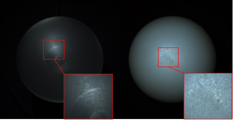
Figure 19: The observed image of Acrylic Ball (left) and Nylon Ball (right) from DiLiGenT$10^{2}$ Dataset [36]. The red squares indicate the regions that may harm the performance of DANI-Net.

Table 9: Quantitative comparison in terms of MAE of surface normal on DiLiGenT$10^{2}$ benchmark dataset [40]. Bold numbers indicates the best results.

Material	Method	Ball	Golf	Spike	Nut	Square	Pentagon	Hexagon	Propeller	Turbine	Bunny	AVG
Nylon	DANI-Net	7.06	20.98	22.63	22.79	25.33	28.3	26.96	24.00	34.37	23.82	23.62
	DANI-Net w rm	5.23	13.40	9.61	16.22	20.43	24.10	19.18	22.62	34.43	19.17	18.44
Acrylic	DANI-Net	34.14	39.13	36.63	35.25	42.70	36.90	44.67	23.50	33.03	21.89	34.78
	DANI-Net w rm	35.27	25.50	35.10	33.38	36.98	36.16	45.61	25.23	32.90	19.27	32.54

Validation of anisotropic material modeling. To validate the effectiveness of our anisotropic material modeling method, we visualize the rendered image, and 4 dominant ASG bases of 2 shapes (i.e., Ball and Bunny) made up of 3 anisotropic materials (i.e., Steel, Cu, and Al respectively), compared with SCPS-NIR [26]’s rendered image and 4 dominant SG bases in Fig. 20. According to the result, our rendered images are more realistic than [26].

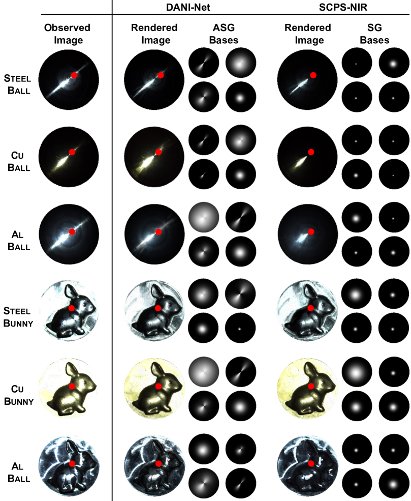
Figure 20: Visualization of the observed images (column 1), rendered images (column 2, 5), ASG bases (column 3, 4) and SG bases (column 6, 7) on Ball and Bunny made up of Steel, Cu, and Al. The rendered images with anisotropic material modeling are generated by DANI-Net (column 2-4). The rendered images with isotropic material modeling are generated by SCPS-NIR [26] (column 5-7).

Appendix E Results on Apple & Gourd Dataset [2] and Light Stage Data Gallery dataset [6]

Preprocessing. For Apple & Gourd, we scale the images into 0.5 of their original size for efficient training. For Light Stage Data Gallery, we use a preprocessing method that is different from [26, 10]. We follow [6] to implement gamma correction with an exponent as $2.2$ on objects with LDR observed images (i.e. objects expect Helmet Front) and magnify the pixel intensity 5 times on objects except Plant because the original pixel intensities on those objects are too low, leading to strong artifacts on the predicted normal map. We also downsample the Plant’s observed images to 0.5 of their original size for efficient training. The above preprocessing process is also applied in [26] for a fair comparison.

Qualitative and Quantitative Results. Table E shows the light calibration results of 3 objects from Apple & Gourd Dataset [2] and 6 objects from Light Stage Data Gallery dataset [6]. As these two datasets don’t release the ground truth normal map, we only provide the predicted normal map in Fig. 21 and Fig. 22 for qualitative analysis. The results show that DANI-Net can not only estimate the surface normal reasonably but also calibrate the light accurately (we have the state-of-the-art light calibration results), illustrating that DANI-Net is free from the deviation of different experimental setups.

Table 10: Quantitative comparison in terms of MAE of light direction and scale-invariant error of intensity on DiLiGenT benchmark dataset [40]. Bold numbers and underlined numbers indicate the best and the second-best results, respectively.

c—cccccc—cccccccccccc—cc Model Apple Gourd1 Gourd2 Plant Helmet Left Helmet Front Knight Kneeling Knight Standing Knight Fighting AVG
dir. int. dir. int. dir. int. dir. int. dir. int. dir. int. dir. int. dir. int. dir. int. dir. int.
PF14 [34] 6.68 0.109 21.23 0.096 25.87 0.329 20.56 0.227 25.40 0.576 81.60 0.133 46.69 9.805 33.81 1.311 69.50 1.137 36.82 1.52
CW20 [10] 10.91 0.094 4.29 0.042 7.13 0.199 10.49 0.154 5.33 0.096 6.22 0.183 14.41 0.181 5.31 0.198 13.42 0.168 8.61 0.146
SCPS-NIR [26] 1.87 0.016 2.34 0.027 2.01 0.233 10.52 0.150 3.96 0.123 3.31 0.138 6.72 0.211 9.09 0.185 11.82 0.299 5.74 0.154
DANI-Net 2.40 0.014 1.50 0.027 0.97 0.227 5.76 0.096 3.90 0.122 4.69 0.094 6.43 0.196 8.88 0.159 6.12 0.147 4.74 0.129

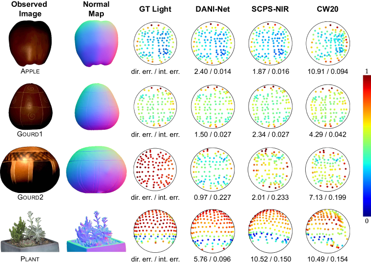
Figure 21: The visual quality comparison among DANI-Net, SCPS-NIR [26], and CW20 [10] on Apple, Gourd1, and Gourd2 from Apple & Gourd [2] and Plant from Light Stage Data Gallery [6] in terms of normal map (column 2) and light map (column 3 - 6). Numbers indicate the MAE (for light directions).

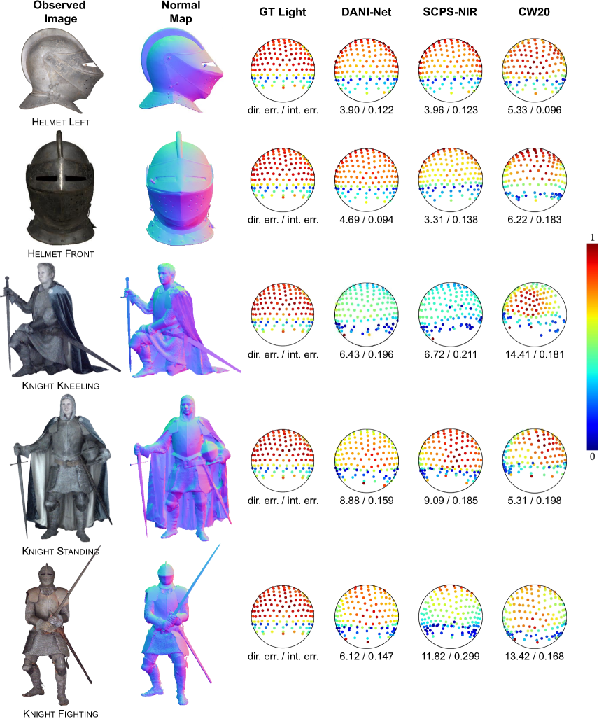
Figure 22: The visual quality comparison among DANI-Net, SCPS-NIR [26], and CW20 [10] on Helmet Left, Helmet Front, Knight Kneeling, Knight Standing and Knight Fighting from Light Stage Data Gallery [6] in terms of normal map (column 2) and light map (column 3 - 6). Numbers indicate the MAE (for light directions).

References

- [1] Jens Ackermann, Fabian Langguth, Simon Fuhrmann, and Michael Goesele. Photometric stereo for outdoor webcams. In Proc. Computer Vision and Pattern Recognition (CVPR), 2012.
- [2] Neil Alldrin, Todd Zickler, and David Kriegman. Photometric stereo with non-parametric and spatially-varying reflectance. In Proc. Computer Vision and Pattern Recognition (CVPR), 2008.
- [3] Svetlana Barsky and Maria Petrou. The 4-source photometric stereo technique for three-dimensional surfaces in the presence of highlights and shadows. In IEEE Transactions on Pattern Analysis and Machine Intelligence (TPAMI), 2003.
- [4] Peter N Belhumeur, David J Kriegman, and Alan L Yuille. The bas-relief ambiguity. In International Journal of Computer Vision (IJCV), 1999.
- [5] Mark Boss, Raphael Braun, Varun Jampani, Jonathan T. Barron, Ce Liu, and Hendrik P.A. Lensch. Nerd: Neural reflectance decomposition from image collections. In Proc. International Conference on Computer Vision (ICCV), 2021.
- [6] Charles-Félix Chabert, Per Einarsson, Andrew Jones, Bruce Lamond, Wan-Chun Ma, Sebastian Sylwan, Tim Hawkins, and Paul Debevec. Relighting human locomotion with flowed reflectance fields. In EGSR, 2006.
- [7] Manmohan Chandraker, Sameer Agarwal, and David Kriegman. Shadowcuts: Photometric stereo with shadows. In Proc. Computer Vision and Pattern Recognition (CVPR), 2007.
- [8] Guanying Chen, Kai Han, Boxin Shi, Yasuyuki Matsushita, and Kwan-Yee K Wong. Self-calibrating deep photometric stereo networks. In Proc. Computer Vision and Pattern Recognition (CVPR), 2019.
- [9] Guanying Chen, Kai Han, and Kwan-Yee K Wong. Ps-fcn: A flexible learning framework for photometric stereo. In Proc. European Conference on Computer Vision (ECCV), 2018.
- [10] Guanying Chen, Michael Waechter, Boxin Shi, Kwan-Yee K Wong, and Yasuyuki Matsushita. What is learned in deep uncalibrated photometric stereo? In Proc. European Conference on Computer Vision (ECCV), 2020.
- [11] Donghyeon Cho, Yasuyuki Matsushita, Yu-Wing Tai, and In So Kweon. Semi-calibrated photometric stereo. In IEEE Transactions on Pattern Analysis and Machine Intelligence (TPAMI), 2018.
- [12] Hin-Shun Chung and Jiaya Jia. Efficient photometric stereo on glossy surfaces with wide specular lobes. In Proc. Computer Vision and Pattern Recognition (CVPR), 2008.
- [13] Athinodoros S Georghiades. Incorporating the torrance and sparrow model of reflectance in uncalibrated photometric stereo. In Proc. International Conference on Computer Vision (ICCV), 2003.
- [14] Dan B Goldman, Brian Curless, Aaron Hertzmann, and Steven M Seitz. Shape and spatially-varying brdfs from photometric stereo. In IEEE Transactions on Pattern Analysis and Machine Intelligence (TPAMI), 2009.
- [15] Shuhei Hashimoto, Daisuke Miyazaki, and Shinsaku Hiura. Uncalibrated photometric stereo constrained by intrinsic reflectance image and shape from silhoutte. In International Conference on Machine Vision Applications (MVA), 2019.
- [16] Steffen Herbort and Christian Wöhler. An introduction to image-based 3d surface reconstruction and a survey of photometric stereo methods. 3D Research, 2011.
- [17] Tomoaki Higo, Yasuyuki Matsushita, and Katsushi Ikeuchi. Consensus photometric stereo. In Proc. Computer Vision and Pattern Recognition (CVPR), 2010.
- [18] Michael Holroyd, Jason Lawrence, Greg Humphreys, and Todd Zickler. A photometric approach for estimating normals and tangents. In ACM TOG, 2008.
- [19] Satoshi Ikehata. Cnn-ps: Cnn-based photometric stereo for general non-convex surfaces. In Proceedings of the European conference on computer vision (ECCV), pages 3–18, 2018.
- [20] Satoshi Ikehata, David Wipf, Yasuyuki Matsushita, and Kiyoharu Aizawa. Robust photometric stereo using sparse regression. In Proc. Computer Vision and Pattern Recognition (CVPR), 2012.
- [21] James T Kajiya. The rendering equation. In Proceedings of the 13th annual conference on Computer graphics and interactive techniques, pages 143–150, 1986.
- [22] James T Kajiya and Brian P Von Herzen. Ray tracing volume densities. In ACM SIGGRAPH computer graphics, 1984.
- [23] Asaf Karnieli, Ohad Fried, and Yacov Hel-Or. Deepshadow: Neural shape from shadow. In Proc. European Conference on Computer Vision (ECCV), 2022.
- [24] David J Kriegman and Peter N Belhumeur. What shadows reveal about object structure. JOSA A, 2001.
- [25] Junxuan Li and Hongdong Li. Neural reflectance for shape recovery with shadow handling. In Proc. Computer Vision and Pattern Recognition (CVPR), 2022.
- [26] Junxuan Li and Hongdong Li. Self-calibrating photometric stereo by neural inverse rendering. In Proc. European Conference on Computer Vision (ECCV), 2022.
- [27] Shichen Liu, Tianye Li, Weikai Chen, and Hao Li. Soft rasterizer: A differentiable renderer for image-based 3d reasoning. In Proc. International Conference on Computer Vision (ICCV), 2019.
- [28] Feng Lu, Xiaowu Chen, Imari Sato, and Yoichi Sato. Symps: Brdf symmetry guided photometric stereo for shape and light source estimation. In IEEE Transactions on Pattern Analysis and Machine Intelligence (TPAMI), 2017.
- [29] Ben Mildenhall, Pratul P Srinivasan, Matthew Tancik, Jonathan T Barron, Ravi Ramamoorthi, and Ren Ng. Nerf: Representing scenes as neural radiance fields for view synthesis. In Proc. European Conference on Computer Vision (ECCV), 2020.
- [30] Yosuke Nakagawa, Hideaki Uchiyama, Hajime Nagahara, and Rin-Ichiro Taniguchi. Estimating surface normals with depth image gradients for fast and accurate registration. In International Conference on 3D Vision, 2015.
- [31] Diego Nehab, Szymon Rusinkiewicz, James Davis, and Ravi Ramamoorthi. Efficiently combining positions and normals for precise 3d geometry. In ACM transactions on graphics (TOG), 2005.
- [32] Michael Oechsle, Songyou Peng, and Andreas Geiger. Unisurf: Unifying neural implicit surfaces and radiance fields for multi-view reconstruction. In Proc. Computer Vision and Pattern Recognition (CVPR), 2021.
- [33] Dave Pagurek and Jerry Yin. Differentiable shadow rendering, 2020.
- [34] Thoma Papadhimitri and Paolo Favaro. A closed-form, consistent and robust solution to uncalibrated photometric stereo via local diffuse reflectance maxima. In International Journal of Computer Vision (IJCV), 2014.
- [35] Xiaojuan Qi, Renjie Liao, Zhengzhe Liu, Raquel Urtasun, and Jiaya Jia. Geonet: Geometric neural network for joint depth and surface normal estimation. In Proc. Computer Vision and Pattern Recognition (CVPR), 2018.
- [36] Jieji Ren, Feishi Wang, Jiahao Zhang, Qian Zheng, Mingjun Ren, and Boxin Shi. Diligent: A photometric stereo benchmark dataset with controlled shape and material variation. In Proceedings of the IEEE/CVF Conference on Computer Vision and Pattern Recognition, pages 12581–12590, 2022.
- [37] Francesco Sarno, Suryansh Kumar, Berk Kaya, Zhiwu Huang, Vittorio Ferrari, and Luc Van Gool. Neural architecture search for efficient uncalibrated deep photometric stereo. In Proc. Winter Conference on Application of Computer Vision (WACV), 2022.
- [38] Steven M Seitz, Brian Curless, James Diebel, Daniel Scharstein, and Richard Szeliski. A comparison and evaluation of multi-view stereo reconstruction algorithms. In Proc. Computer Vision and Pattern Recognition (CVPR), 2006.
- [39] Boxin Shi, Yasuyuki Matsushita, Yichen Wei, Chao Xu, and Ping Tan. Self-calibrating photometric stereo. In Proc. Computer Vision and Pattern Recognition (CVPR), 2010.
- [40] Boxin Shi, Zhe Wu, Zhipeng Mo, Dinglong Duan, Sai-Kit Yeung, and Ping Tan. A benchmark dataset and evaluation for non-lambertian and uncalibrated photometric stereo. In IEEE Transactions on Pattern Analysis and Machine Intelligence (TPAMI), 2016.
- [41] Pratul P. Srinivasan, Boyang Deng, Xiuming Zhang, Matthew Tancik, Ben Mildenhall, and Jonathan T. Barron. Nerv: Neural reflectance and visibility fields for relighting and view synthesis. In Proc. Computer Vision and Pattern Recognition (CVPR), 2021.
- [42] Kalyan Sunkavalli, Todd Zickler, and Hanspeter Pfister. Visibility subspaces: Uncalibrated photometric stereo with shadows. In Proc. European Conference on Computer Vision (ECCV), 2010.
- [43] Tatsunori Taniai and Takanori Maehara. Neural inverse rendering for general reflectance photometric stereo. In Proc. International Conference on Machine Learning (ICML), 2018.
- [44] Dor Verbin, Peter Hedman, Ben Mildenhall, Todd Zickler, Jonathan T Barron, and Pratul P Srinivasan. Ref-nerf: Structured view-dependent appearance for neural radiance fields. In Proc. Computer Vision and Pattern Recognition (CVPR), 2021.
- [45] Bruce Walter. Notes on the ward brdf. Program of Computer Graphics, Cornell University, Technical Report, 2005.
- [46] Peng Wang, Lingjie Liu, Yuan Liu, Christian Theobalt, Taku Komura, and Wenping Wang. Neus: Learning neural implicit surfaces by volume rendering for multi-view reconstruction. In Proc. Conference on Neural Information Processing Systems (NeurIPS), 2021.
- [47] Eva Weigl, Sebastian Zambal, Matthias Stöger, and Christian Eitzinger. Photometric stereo sensor for robot-assisted industrial quality inspection of coated composite material surfaces. In International Conference on Quality Control by Artificial Vision (QCAV), 2015.
- [48] Robert J Woodham. Photometric method for determining surface orientation from multiple images. In Optical Engineering, 1980.
- [49] Lun Wu, Arvind Ganesh, Boxin Shi, Yasuyuki Matsushita, Yongtian Wang, and Yi Ma. Robust photometric stereo via low-rank matrix completion and recovery. In Proc. Asian Conference on Computer Vision (ACCV), 2010.
- [50] Tai-Pang Wu, Kam-Lun Tang, Chi-Keung Tang, and Tien-Tsin Wong. Dense photometric stereo: A markov random field approach. In IEEE Transactions on Pattern Analysis and Machine Intelligence (TPAMI), 2006.
- [51] Zhe Wu and Ping Tan. Calibrating photometric stereo by holistic reflectance symmetry analysis. In Proc. Computer Vision and Pattern Recognition (CVPR), 2013.
- [52] Limin Xie, Zhan Song, Guohua Jiao, Xinhan Huang, and Kui Jia. A practical means for calibrating an led-based photometric stereo system. In Optics and Lasers in Engineering, 2015.
- [53] Wuyuan Xie, Zhan Song, and Ronald C Chung. Real-time three-dimensional fingerprint acquisition via a new photometric stereo means. In Optical Engineering, 2013.
- [54] Yiheng Xie, Towaki Takikawa, Shunsuke Saito, Or Litany, Shiqin Yan, Numair Khan, Federico Tombari, James Tompkin, Vincent Sitzmann, and Srinath Sridhar. Neural fields in visual computing and beyond. In Computer Graphics Forum, 2022.
- [55] Kun Xu, Wei-Lun Sun, Zhao Dong, Dan-Yong Zhao, Run-Dong Wu, and Shi-Min Hu. Anisotropic spherical gaussians. In ACM TOG, 2013.
- [56] Wenqi Yang, Guanying Chen, Chaofeng Chen, Zhenfang Chen, and Kwan-Yee K Wong. Ps-nerf: Neural inverse rendering for multi-view photometric stereo. In Proc. European Conference on Computer Vision (ECCV), 2022.
- [57] Wenqi Yang, Guanying Chen, Chaofeng Chen, Zhenfang Chen, and Kwan-Yee K Wong. -nerf: Neural reflectance field from shading and shadow under a single viewpoint. In Proc. Conference on Neural Information Processing Systems (NeurIPS), 2022.
- [58] Sai-Kit Yeung, Tai-Pang Wu, Chi-Keung Tang, Tony F Chan, and Stanley J Osher. Normal estimation of a transparent object using a video. In IEEE Transactions on Pattern Analysis and Machine Intelligence (TPAMI), 2014.
- [59] Yizhou Yu and Johnny T Chang. Shadow graphs and surface reconstruction. In Proc. European Conference on Computer Vision (ECCV), 2002.
- [60] Alan Yuille and Daniel Snow. Shape and albedo from multiple images using integrability. In Proc. Computer Vision and Pattern Recognition (CVPR), 1997.
- [61] Guangjun Zhang and Zhenzhong Wei. A novel calibration approach to structured light 3d vision inspection. In Optics & Laser Technology, 2002.
- [62] Kai Zhang, Fujun Luan, Qianqian Wang, Kavita Bala, and Noah Snavely. Physg: Inverse rendering with spherical gaussians for physics-based material editing and relighting. In Proc. Computer Vision and Pattern Recognition (CVPR), 2021.
- [63] Xiuming Zhang, Pratul P Srinivasan, Boyang Deng, Paul Debevec, William T Freeman, and Jonathan T Barron. Nerfactor: Neural factorization of shape and reflectance under an unknown illumination. In ACM TOG, 2021.
- [64] Qian Zheng, Ajay Kumar, Boxin Shi, and Gang Pan. Numerical reflectance compensation for non-lambertian photometric stereo. IEEE Transactions on Image Processing (TIP), 2019.
- [65] Qian Zheng, Boxin Shi, and Gang Pan. Summary study of data-driven photometric stereo methods. Virtual Reality & Intelligent Hardware, 2020.
- [66] Zhenglong Zhou and Ping Tan. Ring-light photometric stereo. In Proc. European Conference on Computer Vision (ECCV), 2010.