Towards secure judgments aggregation in AHP

Abstract

In decision-making methods, it is common to assume that the experts are honest and professional. However, this is not the case when one or more experts in the group decision making framework, such as the group analytic hierarchy process (GAHP), try to manipulate results in their favor. The aim of this paper is to introduce two heuristics in the GAHP, setting allowing to detect the manipulators and minimize their effect on the group consensus by diminishing their weights. The first heuristic is based on the assumption that manipulators will provide judgments which can be considered outliers with respect to those of the rest of the experts in the group. The second heuristic assumes that dishonest judgments are less consistent than the average consistency of the group. Both approaches are illustrated with numerical examples and simulations.

1 Introduction

Group decision making refers to the situations where the problem of selecting the best alternative (option, solution, etc.) is handled collectively by a set of individuals, preferably experts in the field. Usually, such processes involve complex problems, too difficult to be handled by an individual, or they deal with actions legally required to be made by a collective. These situations include government meetings, various board negotiations, policy making, business dealings, complex laboratory experiments, elections, jury trials, reaching consensus in social networks, and many others. The fundamentals of group decision making can be found e.g. in [6, 11, 18, 26, 28, 37, 38, 46].

One of the problems associated with group decision making (GDM) is that it is susceptible to manipulation if one or more experts try to influence the group outcome in their favor by, for example, providing dishonest judgments. The manipulation, especially in the political context, can be traced back at least to the ancient societies of Greece and Rome, see e.g. [7]. More recently, a description of political manipulation in a GDM setting can be found, for example, in the work of Maoz [40], who investigated examples of U.S. and Israeli foreign policy choices under crisis conditions, or Hoyt [25], who examined the American decision process during the Iranian revolution. Analysis of manipulation in selected voting methods can be found e.g. in [4, 19, 20, 39, 49, 51]. Further on, Faliszewski et al. [15, 14] proposed different approaches of manipulation protection in the context of elections.

Another area of group decision making vulnerable to manipulation are social networks. An approach to prevent weight manipulation by minimum adjustment and maximum entropy method in social network group decision making can be found in [50]. Similarly, Wu et al. [52] introduced a novel framework to prevent manipulative behaviors during consensus-reaching processes in social network group decision making. They considered two means of manipulation – individual manipulation, where each expert manipulates his/her own behavior to achieve higher importance (weight); and group manipulation, where a group of experts forces inconsistent experts to adopt specific recommendation advices – and investigated models to counteract both of them. Manipulation in multiple-criteria group decision making attracted the attention of several recent studies. Dong et al. [12] presented a new strategic manipulation called trust relationship manipulation and discussed clique-based strategies to manipulate trust relationships to obtain the desired ranking of the alternatives. Hnatiienko [24] studied the problem of manipulating the choice of decision options in peer review processes and proposed a classification of selection manipulation problems in experts’ evaluation. Lev and Lewenberg [36] investigated cases when agents may wish to re-draw the organizational chart of a company, or markets (which is called ‘reverse gerrymandering’), to maximize their influence across the company’s sub-units, or to allocate resources to the desired areas. Yager [53, 54] studied methods of strategic manipulation of preferential data. He proposed modification of the preference aggregation function in such a way that the attempts of individual agents to manipulate the data are penalized. Dong et al. [10] defined the concept of the ranking range of an alternative in multiple-attribute decision making and proposed a series of mixed binary linear programming models to show the process of designing a strategic attribute weight vector. Moreover, the authors studied the conditions to manipulate a strategic attribute weight based on the ranking range and the proposed model. Sasaki [48] discussed the issue of strategic manipulation in the context of group decision making with pairwise comparisons. The author considered a scenario of group decision-making situations formulated as strategic games and his theoretical results show truthful judgments (pairwise comparisons) can be a dominant strategy only in very few situations.

Apart from the last study, the problem of manipulation in pairwise comparison methods has not as yet been studied thoroughly. This paper aims to fill the aforementioned gap and focuses on group decision making in the analytic hierarchy process (GAHP), along with the problem of possible manipulation of its outcome. In the GAHP setting, a group of experts provides pairwise comparisons of alternatives under consideration with the aim of selecting the best alternative, see e.g. Dong and Saaty [9], Ramanathan and Ganesh [42], or Saaty [46]. The aim of the paper is to introduce two heuristics in the GAHP setting to detect the manipulators and minimize their effect on the group consensus by minimizing their weights. The first heuristic is based on the assumption that manipulators will provide judgments which can be considered outliers with respect to judgments of the rest of the experts in the group. The second one assumes that dishonest judgments are less consistent than the average consistency of the group. Both approaches are illustrated with numerical examples and simulations.

The paper is composed of five sections. The Introduction (Sec. 1) and Preliminaries (Sec. 2) aim to introduce the reader to the literature on the subject and recall the necessary concepts and definitions of the quantitative and qualitative pairwise comparisons method. The following section, Inconsistency Driven Pairwise Ranking Aggregation (Sec. 3), identifies the problem of ranking manipulation and introduces the proposed robust methods of aggregating results coming from various experts. Sec. 4 contains two Montecarlo experiments allowing to assess the effectiveness of the proposed methods. The paper ends with (Sec. 5), containing a short summary of the achieved results.

2 Preliminaries

2.1 Pairwise comparisons

Comparing alternatives in pairs serves as the basis of many decision-making methods, including AHP, BWM, HRE, MACBETH and others [45, 43, 30, 3]. In these methods, the results of the comparisons constitute the decision-making data that are subject to further processing. Let $A=\{a_{1},\ldots,a_{n}\}$ be a finite set of alternatives (available options that each expert can choose) and $E=\{e_{1},\ldots,e_{k}\}$ be the set of experts involved in the decision-making process. Similarly, let $C_{q}=\left\{c_{ijq}\in\mathbb{R}_{+}\,:\,i,j=1,\ldots,n\right\}$ be a set of pairwise judgments provided by the $q$-th expert, so that $c_{ijq}$ is the relative importance of $a_{i}$ with respect to $a_{j}$ according to the opinion of $e_{r}$. It is convenient to represent the set of judgments as a pairwise comparisons (PC) matrix $C_{q}=(c_{ijq})$. For the sake of readability, however, we will try to leave the additional index $q$ wherever it is not necessary, i.e. when the expert’s number is irrelevant. In such a case, the PC matrix takes the form $C=(c_{ij})$. PC matrix entries can be interpreted as ratios of individual priorities. Thus, when for some PC matrix $C$ it holds that $c_{ij}=x$, we mean that our expert decided that $a_{i}$ is $x$ times more important than $a_{j}$. For the same reason, $c_{ij}=1$ means that both compared alternatives are equally preferred. The diagonal of $C$ contains the results of comparisons of alternatives with themselves, i.e. it is filled with $1$’s. Similarly, in most cases we may expect that $c_{ij}=c_{ji}^{-1}$, i.e. that the matrix is reciprocal.

Definition 1.

A PC matrix $C=(c_{ij})$ is said to be reciprocal if for every $c_{ij}$ holds $c_{ij}=c_{ji}^{-1}$.

The purpose of the decision-making methods is to prepare recommendations. It usually takes the form of a numerical ranking that assigns some real-number values to the alternatives.

Definition 2.

Let $A$ be a set of alternatives. The numerical ranking function for $A$ is a mapping $w:A\rightarrow\mathbb{R}_{+}$ assigning a real and positive number to each alternative.

The numerical ranking takes the form of a weight (priority) vector $w$:

$$w=\left[w(a_{1}),\ldots,w(a_{n})\right]^{T}.$$

In the literature we may find more than a dozen methods allowing us to determine the priority vector [32, 41]. The most popular ones are EVM (Eigenvalue Method) and GMM (Geometric Mean Method) [45, 8]. According to the former, the ranking vector is calculated as the normalized principal eigenvector. Thus, having the solution of equation

$$C\widehat{w}=\lambda_{\textit{max}}\widehat{w}$$

where $\lambda_{\textit{max}}$ is a principal eigenvalue of $C$, the entries of the priority vector $w_{\textit{ev}}=\left[w_{\textit{ev}}(a_{1}),\ldots,w_{\textit{ev}}(a_{n})\right]^{T}$ are given as

$$w_{\textit{ev}}(a_{i})=\frac{\widehat{w}(a_{i})}{\sum_{j=1}^{n}\widehat{w}(a_{j})}.$$

In the case of the latter, although the assumptions of the procedure are similar [33], the calculations are simpler. In this approach, the entries of a priority vector $w_{\textit{gm}}=\left[w_{\textit{gm}}(a_{1}),\ldots,w_{\textit{gm}}(a_{n})\right]^{T}$ have the form:

$$w_{\textit{gm}}(a_{i})=\frac{s_{i}}{\sum_{j=1}^{n}s_{j}},$$

where

$$s_{i}=\left(\prod_{j=1}^{n}c_{ij}\right)^{1/n}.$$

Thus, the individual priorities of alternatives are just geometric means of rows of a PC matrix. Both of the aforementioned methods have their incomplete versions [22, 31], i.e. procedures that allow to calculate the priority vector even if not all entries of $C$ are known.

2.2 Inconsistency

Comparing alternatives pairwise is easier than comparing more alternatives at the same time. However, if one makes comparisons independently, it may lead to inconsistency (and it usually does).

Definition 3.

A PCM $C$ is consistent [32] if for every $i,j,k=1,\ldots,n$ holds

$$c_{ik}c_{kj}=c_{ij}.$$

It is fairly easy to prove that it is equivalent to the existence of a positive vector $w$ such that for every $i,j=1,\ldots,n$

$$c_{ij}=\frac{w(a_{i})}{w(a_{j})}.$$ (1)

In real-world applications, inconsistent PCMs appear naturally. Nonetheless, the level of inconsistency should not be too high, as it may lead to several problems. These may include impaired sensitivity of data [34], or lack of trust in the experts’ competence, leading to the method being perceived as unreliable. Therefore plenty of inconsistency indicators have been defined in the literature. One of the most popular is the Consistency Index introduced by Saaty in Saaty [45]:

Definition 4.

The Consistency Index of a $n\times n$ PC matrix $C=[c_{ij}]$ is given by

$$\textit{CI}(C)=\frac{\lambda_{max}-n}{n-1},$$

where $\lambda_{\textit{max}}$ is the principal right eigenvalue of $C$ (i.e. the maximum one according to the absolute value).

The index $\textit{CI}(C)$ is zero if $C$ is consistent. Otherwise, it is positive, and more specifically $0\leq\textit{CI}(C)\leq(q-1)^{2}/2q$ where $1/q\leq c_{ij}\leq q$, for $i,j=1,\ldots,n$ [2, 32, p. 103].

Another interesting inconsistency indicator has been proposed by Koczkodaj [29].

Definition 5.

The Koczkodaj’s inconsistency index of PC matrix $C$ is defined as

$$K(C)=\max\left\{K_{ijk}:1\leq i<j<k\leq n\right\},$$

where

$$K_{ijk}=\min\left\{\left|1-\frac{c_{ik}c_{kj}}{c_{ij}}\right|,\left|1-\frac{c_{ij}}{c_{ik}c_{kj}}\right|\right\}.$$

The difference between the two indices is that the latter is not related to the priority deriving method, while the first one contains a reference to the principal eigenvector of $C$. Both indices have their versions for incomplete matrices [35]. Very often, $K(C)$ is considered a local inconsistency indicator, while CI(C) is called global consistency index [32].

Ranking vectors can be compared in many ways. Depending on whether the comparison is quantitative or qualitative, the appropriate metric is used. A convenient way to compare two ordinal ranking vectors is the Kendall Tau distance [27, 34].

Definition 6.

The Kendall Tau distance for two ordinal ranking vectors $u$ and $v$ is defined as

$$K_{\textit{rd}}(u,v)=\frac{2K_{d}(u,v)}{n(n-1)},$$ (2)

where

$$K_{d}(u,v)=\left|\left\{(i,j)\,\text{s.t.}\,i<j\,\wedge\,\textit{sign}\left(u(a_{i})-u(a_{j})\right)\neq\textit{sign}\left(v(a_{i})-v(a_{j})\right)\right\}\right|.$$ (3)

$K_{d}(u,v)$ counts the number of pairwise swaps that distinguish two vectors. For example if $u=(1,2,3)$ and $v=(2,1,3)$ then $K_{d}(u,v)=1$, as only one swap between $1$ and $2$ is needed to transform vector $v$ to vector $u$. Due to the similarity of this idea to the so-called bubble sort algorithm, this value is sometimes called the bubble-sort distance.

It is easy to see that for the most distant two vectors $u$ and $v$ where $\left|u\right|=\left|v\right|=n$, the value of $K_{d}(u,v)=n(n-1)/2$ (in such a case, $u$ contains the elements of $v$ in reverse order). Thus, the normalized Kendall distance of two ordinal vectors takes its final form (2), where for the most distant vectors $u,v$ the value $K_{\textit{rd}}(u,v)=1$. It is worth noting that $K_{\textit{rd}}$ does not depend on the number of alternatives in the ranking.

For quantitative rankings, any measure of vector distance can be used to determine their distance. For the purpose of this article we use the Manhattan distance; however, the Chebyshev distance [23] is also common in the literature.

Definition 7.

The Manhattan distance between two cardinal ranking vectors $u$ and $v$ is defined as

$$M_{d}(u,v)=\sum_{i=1}^{n}\left|u(a_{i})-v(a_{i})\right|.$$

Providing that all the entries of both $u$ and $v$ sum up to $1$, the result $M_{d}(u,v)\leq 2$.

2.3 Group Decision Making

In a situation where many experts work on a recommendation and each of them presents their own PC matrix, these data must be aggregated. Typically, arithmetic or geometric weighted averages are used for aggregation, although there are strong axiomatic arguments for using geometric mean for this purpose [1]. Hence, in our further considerations, we will focus on this very method.

We can aggregate either entire PC matrices or priority vectors resulting from these matrices. The first approach is called AIJ (Aggregation of Individual Judgments) while the second is referred to as AIP (Aggregation of Individual Priorities [16]). Let us consider a group of experts $E=\{e^{1},\ldots,e^{k}\}$ whose task is to compare a set $A=\{a_{1},\ldots,a_{n}\}$ of alternatives pairwise. Each of them provides a PC matrix $C_{q}=[c_{ijq}]$ containing its personal judgements on elements of $A$. In the AIJ approach, we begin by creating the aggregated matrix

$$C=\left[\begin{array}[]{cccc}1&\prod_{q=1}^{k}c_{12q}^{r_{q}}&\cdots&\prod_{q=1}^{k}c_{1nq}^{r_{q}}\\ \vdots&1&\vdots&\vdots\\ \vdots&\vdots&\ddots&\vdots\\ \prod_{q=1}^{k}c_{n1q}^{r_{q}}&\cdots&\cdots&1\end{array}\right],$$

where $r_{1},\ldots,r_{k}\in[0,1]$ and $\sum_{q=1}^{k}r_{q}=1$. Then, adopting $C$ as input, we calculate the final priority vector using the method we prefer. The values $r_{1},\ldots,r_{k}$ represent the priorities assigned to individual experts. They correspond to the strength of the influence of individual experts’ opinions on the final result. In a situation where the opinion of each of the experts has the same impact (which is usually the case), $r_{q}=1/k$ for $q=1,\ldots,k$.

In the AIP approach, first, for each $C_{q}$, we calculate a priority vector

$$w_{q}=\left[w_{q}(a_{1}),\ldots,w_{q}(a_{n})\right]^{T}.$$

Then, we aggregate the vectors so that the resulting ranking is given as

$$w=\left[w(a_{1}),\ldots,w(a_{n})\right]^{T},$$

where

$$w(a_{i})=\frac{\prod_{q=1}^{k}w_{q}^{r_{q}}(a_{i})}{\sum_{i=1}^{n}\prod_{q=1}^{k}w_{q}^{r_{q}}(a_{i})}.$$ (4)

Similarly as before, the higher value of $r_{q}$, the stronger impact of the $q$-th expert on the final recommendation.

3 Inconsistency-Driven Pairwise Ranking Aggregation

3.1 Problem statement

In decision-making methods, it is common to assume the honesty and professionalism of experts. According to the first of these assumptions, each of the experts will try to express opinions that are as close to the actual state as possible. In other words, they will not express an opinion that is contrary to their own knowledge and inner conviction. Their alleged professionalism, on the other hand, allows us to believe that the assessment made by experts will be reliable and based on a possibly objective comparison of various considered options. Both of these assumptions allow us to hope that the judgments of different yet honest and professional experts should rather coincide. Therefore, outliers are likely to be either dishonest or unprofessional. In either case, there is good reason to reduce the impact of such opinions on the final result.

Describing the facts and fiction about AHP [17, p. 22], Forman notes that “It is possible to be perfectly consistent but consistently wrong.” Paraphrasing this quote, one might say that it is possible to be perfectly consistent and completely dishonest. Nevertheless, in practice, when there are many alternatives and little time to decide, the questions are asked in a random order and the expert does not have the opportunity to learn about the set of alternatives beforehand, the risk of obtaining consistent but insincere answers does not seem very high. Hence, we can expect the insincere expert to give answers less consistent than the average. This leads to the formulation of a second possible heuristic that may point to dishonest or incompetent experts. Too high an inconsistency in an expert’s response may be a good reason to reduce their impact on the final ranking values.

The above observations allow us to propose two procedures for prioritizing experts, so that potentially dishonest experts receive a lower priority than others. The first procedure will be based on the deviation from the average (i.e. it will detect outliers in terms of the preferences presented) (Sec. 3.2). The second one will take the inconsistency in the context of a certain average inconsistency (Sec. 3.3) into account. We are also considering a combination of both of these heuristics (Sec. 3.4).

Example

One of the common variants of manipulation in the social choice theory is control [4]. It is usually carried out by the election organizer. Paradigmatic examples of control include adding or deleting voters. A similar effect can be seen with the pairwise comparison method. Hence, by adding or removing experts, one can try to affect the ranking results. Let us consider the example where the opinion of six experts $e_{1},\ldots,e_{6}$ was taken into account in order to develop recommendations on the four alternatives under consideration. The experts’ opinions were in the form of $4\times 4$ matrices:

$$C_{1}=\left(\begin{array}[]{cccc}1.&1.322&1.926&2.0784\\ 0.7566&1.&1.63&2.6057\\ 0.5192&0.6136&1.&1.011\\ 0.4811&0.3838&0.9888&1.\end{array}\right),$$

$$C_{2}=\left(\begin{array}[]{cccc}1.&1.335&2.408&3.2864\\ 0.749&1.&2.0619&1.619\\ 0.4153&0.485&1.&1.599\\ 0.3043&0.6178&0.6255&1.\end{array}\right),$$

$$C_{3}=\left(\begin{array}[]{cccc}1.&1.034&2.0437&2.6168\\ 0.9668&1.&1.956&1.987\\ 0.4893&0.5113&1.&1.32\\ 0.3821&0.5034&0.7574&1.\end{array}\right),$$

$$C_{4}=\left(\begin{array}[]{cccc}1.&1.3&2.1679&2.0552\\ 0.7691&1.&1.603&2.5181\\ 0.4613&0.624&1.&1.005\\ 0.4866&0.3971&0.9949&1.\end{array}\right),$$

$$C_{5}=\left(\begin{array}[]{cccc}1.&1.052&2.1005&2.5668\\ 0.9501&1.&2.025&1.646\\ 0.4761&0.4938&1.&1.564\\ 0.3896&0.6074&0.6394&1.\end{array}\right),$$

$$C_{6}=\left(\begin{array}[]{cccc}1.&1.153&2.2591&2.4132\\ 0.8669&1.&1.832&1.629\\ 0.4426&0.5459&1.&1.284\\ 0.4144&0.6137&0.7785&1.\end{array}\right).$$

The normalized weight vectors obtained by GMM are as follows:

$$w_{1}=\left[0.355802,0.314085,0.176758,0.153356\right]^{T},$$

$$w_{2}=\left[0.409827,0.285829,0.171231,0.133114\right]^{T},$$

$$w_{3}=\left[0.356504,0.323638,0.176235,0.143623\right]^{T},$$

$$w_{4}=\left[0.362966,0.31053,0.171584,0.154919\right]^{T},$$

$$w_{5}=\left[0.360622,0.311708,0.181946,0.145724\right]^{T},$$

$$w_{6}=\left[0.371263,0.297355,0.174992,0.156391\right]^{T},$$

which means that the six experts indicate $a_{1}$ as the best alternative. Their aggregated ranking is

$$w_{1-6}=\left[0.369045,0.306942,0.175421,0.147627\right]^{T}.$$

However, a dishonest organizer (process facilitator) added two more experts $e_{7}$ and $e_{8}$ who lobby for $a_{2}$. As they know that $a_{1}$ is its main competitor, they proposed opinions (matrices $C_{7}$ and $C_{8}$) i.e.:

$$C_{7}=\left(\begin{array}[]{cccc}1.&0.1752&0.5622&0.3212\\ 5.7078&1.&2.584&1.604\\ 1.779&0.387&1.&1.785\\ 3.1135&0.6236&0.5602&1.\end{array}\right),$$

$$C_{8}=\left(\begin{array}[]{cccc}1.&0.4551&0.2515&0.5273\\ 2.1971&1.&2.0847&2.2497\\ 3.9758&0.4797&1.&1.47\\ 1.896&0.4445&0.6803&1.\end{array}\right),$$

resulting in a ranking downgrading $a_{1}$ and boosting $a_{2}$:

$$w_{7}=\left[0.0897127,0.469102,0.223955,0.21723\right]^{T},$$

$$w_{8}=\left[0.0897127,0.469102,0.223955,0.21723\right]^{T}.$$

Then, applying the standard aggregation process [16, 21], the final ranking is as follows:

$$w_{1-8}=\left[0.266227,0.334807,0.192645,0.160465\right]{}^{T}.$$

This determines the order of alternatives: $a_{2},a_{1},a_{3},a_{4}$ which is in line with the expectations of experts $e_{7}$ and $e_{8}$.

3.2 Preferential distance-driven expert prioritization

Let $\widehat{w}_{i}=\left[\widehat{w}_{i}(a_{1}),\ldots,\widehat{w}_{i}(a_{k})\right]^{T}$ be the ranking vector calculated using either EVM or GMM (Sec. 2.1), based on the matrix $C_{i}$ provided by the expert $e_{i}$ for $i=1,\ldots,k$. Similarly, let $\widehat{w}=\left[\widehat{w}(a_{1}),\ldots,\widehat{w}(a_{n})\right]^{T}$ be a ranking vector calculated using AIP (Sec. 2.3), based on $\widehat{w}_{1},\ldots,\widehat{w}_{k}$. According to the adopted heuristics, the more the opinion of the $i$-th expert differs from that of the entire team, the greater the risk of manipulation. Thus, let

$$\textit{d}_{i}=\left|\widehat{w}-\widehat{w}_{i}\right|$$ (5)

be a quantitative distance between vectors $\widehat{w}$ and $\widehat{w}_{i}$. Then, we need to map the individual distances $d_{i}$ (5) to priority values over a certain numerical scale. For this purpose, let us denote the minimum and maximum of the values $D=\{d_{1},\ldots,d_{k}\}$ as $d_{\textit{min}}$ and $d_{\textit{max}}$ correspondingly. As $d_{\textit{min}}$ corresponds to the most preferred expert and $d_{\textit{min}}$ corresponds to the least preferred expert, we assign the value $h\in\mathbb{R}_{+}$ to $d_{\textit{min}}$ and $l\in\mathbb{R}_{+}$ to $d_{\textit{max}}$, where of course $h>l$. The ratio $h/l$ should correspond to the ratio between the reliability of the expert corresponding to $d_{\textit{min}}$ to the reliability of the expert corresponding to $d_{\textit{max}}$. Values $l$ and $h$ form a scale to which all the distances $d_{1},\ldots,d_{k}$ will be transformed.

Let $f:\mathbb{R}_{+}\rightarrow\mathbb{R}$ be a mapping transforming distances $d_{i}$ to priorities, which after normalization can be used in the weighted AIP procedure. Function $f$ should pass through two points $X=(d_{\textit{min}},h)$ and $Y=(d_{\textit{max}},l)$, so that the highest priority value $h$ is assigned to the expert whose opinion was closest to the mean, and the lowest priority value $l$ is assigned to the expert whose opinion was the farthest from the mean.

The mapping $f$ lets us use a linear function passing through two points $X=(x_{1},x_{2})$ and $Y=(y_{1},y_{2})$ in the form

$$f_{XY}(x)=\frac{x_{2}-y_{2}}{x_{1}-y_{1}}x+\left(x_{2}-\frac{x_{2}-y_{2}}{x_{1}-y_{1}}x_{1}\right).$$ (6)

This allows us to calculate the values $f(d_{1}),\ldots,f(d_{k})$ which determines the priorities of experts $e_{1},\ldots,e_{k}$. In order to satisfy the form of the weighted geometric mean, one would need to rescale the priority values so that they sum up to one. Hence, the final experts’ priorities take the form:

$$r_{i}=\frac{f(d_{i})}{\sum_{i=1}^{k}f(d_{i})},\,\,\,i=1,\ldots,k.$$ (7)

After computing $r_{1},\ldots,r_{k}$, we calculate the final priority vector $w=\left[w(a_{1}),\right.$ $\ldots$ $\left.,w(a_{n})\right]^{T}$ using the weighted version of AIP (4).

For the purpose of the aforementioned example (see end of Section 3.1), let us assume that the expert with the lowest value $d_{\textit{min}}$ is strongly more credible than the expert with the highest value $d_{\textit{max}}$. Following the fundamental scale the ratio $h/l=5$, so we may assign $h=5$ and $l=1$. As a result, we get the linear mapping function $f(x)=-15.0607x+7.0075$, determining the experts’ weights (Fig. 1).

Figure 1: Linear function mapping distances to priorities passing points $(min,h)$ and $(max,l)$.

The weight values are therefore:

$$\left[f(d_{1}),\ldots,f(d_{8})\right]^{T}=\left[5.,3.37,4.97,4.78,4.85,4.53,1.,1.65\right]^{T}.$$

Rescaling produces the values that can be used as the input to the AIP procedure:

$$\left[r_{1},\ldots,r_{8}\right]^{T}=\left[0.165,0.11,0.16,0.15,0.16,0.15,0.0331,0.054\right]^{T}.$$

After re-aggregating the results, we get a priority vector:

$$w_{1-8}=\left[0.327,0.317,0.182,0.152\right]^{T}.$$

As we can see, the alternative $a_{1}$ with the priority $w_{1-8}(a_{1})=0.327$, which is preferred by the majority of voters, returned to the winning position.

3.3 Inconsistency-driven expert prioritization

Instead of using the distance between individual judgment vectors and its mean value, we may use the distance between the inconsistencies of individual experts and the average inconsistency of their judgments. Thus, let

$$d_{i}=\left(I(C_{i})-\frac{1}{k}\sum_{j=1}^{k}I(C_{j})\right),$$

where $I$ is some selected inconsistency index [5, 35]. Contrary to the previous case, in which the distance of the individual ranking from the average value was important, here we have to measure whether the inconsistency of a given expert is below or above the average. If it is above average, it may mean either an attempt (perhaps a naive one) to manipulate the deficiencies of the expert himself (lack of experience, lack of firmness, distraction, time pressure, etc.). However, if the individual ranking is below average, i.e., the expert’s consistency is higher than the average, this may, to some extent, be in favor of the expert. On the other hand, a certain degree of inconsistency is considered desirable [47, p. 265] or [44, p. 172]. In other words, both too high and too small a degree of inconsistency may indicate strategic decision-making, although it is quite difficult to “punish” too much consistency.

These two observations lead to the conclusion that the mapping of distances to priorities should differ depending on the sign of $d_{i}$. Providing that at least two matrices $C_{i}$ and $C_{j}$ such that $I(C_{i})\neq I(C_{j})$ exist, there must exist also two matrices such that $I(C_{p})<1/k\sum_{j=1}^{k}I(C_{j})<I(C_{\textit{q}})$. Let the inconsistency values for the most consistent $e_{\textit{min}}$ and inconsistent $e_{\textit{max}}$ expert be: $I_{\textit{min}}=\min_{j=1,\ldots,k}I(C_{j})$ and $I_{\textit{max}}=\max_{j=1,\ldots,k}I(C_{j})$. Additionally, let $I_{\textit{mid}}$ be the value of inconsistency of the expert whose opinions’ consistency is closest to the average, i.e. $I_{\textit{mid}}=I(C_{i})$ such that $\left|I(C_{i})-1/k\sum_{j=1}^{k}I(C_{j})\right|$ is minimal.

In the next step, we should set the high, middle and low weights, i.e. $h,m$ and $l$ corresponding to the values of $I_{\textit{min}},I_{\textit{mid}}$ and $I_{\textit{max}}$. Thus, we perform three comparisons of experts’ credibility, which result in the following matrix:

$$\textit{C}_{\textit{ex}}=\left(\begin{array}[]{ccc}1&\textit{c}_{\textit{min},\textit{mid}}&\textit{c}_{\textit{min},\textit{max}}\\ 1/\textit{c}_{\textit{min},\textit{mid}}&1&\textit{c}_{\textit{mid},\textit{max}}\\ 1/\textit{c}_{\textit{min},\textit{max}}&1/\textit{c}_{\textit{mid},\textit{max}}&1\end{array}\right).$$ (8)

It is worth noting that in this heuristic, the smaller the inconsistency, the better the results, assuming that $\textit{c}_{\textit{min},\textit{mid}}$, $\textit{c}_{\textit{mid},\textit{max}}$ and $\textit{c}_{\textit{min},\textit{max}}$ cannot be greater than $1$.

Calculating a ranking based on (8) brings us the desired values of $h,m$ and $l$. These allow us to formulate three points through which the function mapping the distance $d_{i}$’s to the weight values of individual experts should pass. These points are: $A=(d_{\textit{min}},h)$, $B=(d_{\textit{mid}},m)$ and $C=(d_{\textit{max}},l)$.

As mapping $f:\mathbb{R}_{+}\rightarrow\mathbb{R}$ transforming distances $I_{i}$ to priorities let us use a piecewise linear function including two segments: $A-B$ and $B-C$. Thus,

$$f_{\textit{XYZ}}(x)=\begin{cases}f_{\textit{XY}}(x)&x<0\\ f_{\textit{YZ}}(x)&x\geq 0\end{cases}.$$

Similarly as before, $f_{\textit{ABC}}=f$ allows us to calculate the values $f(d_{1}),\ldots,f(d_{k})$ which, after appropriate rescaling (7), form the experts’ priorities $r_{1},\ldots,r_{k}$. Finally, the ranking is calculated, taking into account the priorities of individual experts.

In the case of Example 3.1 experts $e_{1},\ldots,e_{8}$ achieved the following consistency values:

$$w_{\textit{cexp}}=\{0.0101,0.0152,0.0026,0.0088,0.013,0.0049,0.0528,0.0519\}$$

It is easy to see that $I_{\textit{min}}=0.0026$ (expert $e_{3}$) and $I_{\textit{max}}=0.0528$ (expert $e_{7}$). The average inconsistency is $0.02$, thus the nearest inconsistency result was achieved by the expert $e_{2}$ with $I_{\textit{mid}}=0.0152$. In the next step, we need to compare the credibility of $e_{3},e_{2}$ and $e_{7}$. Let

$$C_{\textit{ex}}=\left(\begin{array}[]{ccc}1&2&7\\ \frac{1}{2}&1&4\\ \frac{1}{7}&\frac{1}{4}&1\end{array}\right),$$

which yields the following credibility values: $0.603,0.315$ and $0.082$. This allows us to construct the mapping $f_{XYZ}$ (Fig. 2) where $A=(0.0026,0.603)$, $B=(0.02,0.315)$ and $C=(0.082,0.082)$.

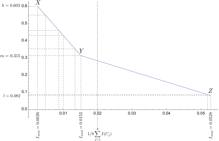
Figure 2: Piecewise linear function mapping distances to priorities passing points $A,B$ and $C$.

According to the function $f_{\textit{XYZ}}=f$, experts $e_{1},\ldots,e_{8}$ obtain the following weights:

$$\left[f(d_{1}),\ldots,f(d_{8})\right]^{T}=[0.432,0.315,0.602,0.462,0.354,0.551,0.082,0.088]^{T}.$$

After rescaling so that all weights sum up to $1$, we obtain the values that can be used as the input to the AIP procedure:

$$\left[r_{1},\ldots,r_{8}\right]^{T}=\left[0.149,0.109,0.208,0.159,0.122,0.19,\ 0.028,0.03\right]^{T}.$$

Then, re-aggregation of experts’ results leads to the final priority vector:

$$w_{1-8}=\left[0.339,0.314,0.1793,0.151\right]^{T}.$$

The alternative $a_{1}$ with the priority $w_{1-8}(a_{1})=0.329$ has the highest rank, whilst $a_{2}$ correctly takes the second place. Thanks to the introduction of priorities, it was again possible to mitigate the manipulation.

3.4 Mixed expert prioritization

It is possible to use both of the above heuristics simultaneously. So let $r_{i}^{1}$ be the weight of the $i$-th expert calculated on the basis of the heuristic distance from the mean judgment (Sec. 3.2), while $r_{i}^{2}$ is the weight of the expert calculated from the difference in inconsistencies (Sec. 3.3). Thus, the mixed expert weight is the linear combination of both:

$$r_{i}=\beta r_{i}^{1}+(1-\beta)r_{i}^{2},\,\,\text{for}\,\,i=1,\ldots,k,$$

where $0\leq\beta\leq 1$ is the coefficient determining the impact of both heuristics. Since $\sum_{i=1}^{k}r_{i}^{1}=\sum_{i=1}^{k}r_{i}^{2}=1$, then also $\sum_{i=1}^{k}r_{i}=1$. Thus, the obtained weights $r_{1},\ldots,r_{k}$ fit the definition of the weighted geometric mean.

In case of Example 3.1 and assuming that both heuristics contribute equally to the weights of the experts, i.e. $\beta=0.5$, we get

$$\left[r_{1},\ldots,r_{8}\right]^{T}=\left[0.157,0.11,0.186,0.159,0.141,0.17,\ 0.03,0.042\right]^{T},$$

which results in the following priority vector:

$$w_{1-8}=\left[0.333,0.316,0.18,0.151\right]^{T}.$$

3.5 The degree of expert’s credibility

In each of the two heuristics described above (Section 3.2 and 3.3), two or three key experts are first selected for credibility assessment. Then, based on this result, a mapping is proposed to prioritize all experts. The credibility evaluation must be made in accordance with the adopted heuristics, i.e. experts less consistent in their judgments or more distant from the average than the competitor have to get the lower score. This may result in a certain inconvenience for those assessing the credibility of experts. They may focus on their attitude towards individual experts, and not on the quality of their expertise. As a result, a person who is liked and popular in the society may get a better assessment than an expert who is reliable but not sociable.

The way to avoid this trap is to provide a procedure that allows us to prioritize key experts without explicitly comparing them. Then, we can assume a priori that the ratio of the best to the worst expert (the first heuristic, Section 3.2) is e.g. $5:1$, or ratios of the best, average and worst experts (the second heuristic, Section 3.3) is e.g. $9:4:1$.

It is also possible to determine these relations in a procedural/functional way. For instance, in the case of our example and the second heuristic, we may assume that the expert priority should be linearly correlated with inconsistency. Thus, as $d_{\textit{min}}=0.0026$, $d_{\textit{mid}}=0.0152$ and $d_{\textit{max}}=0.0528$ (Section 3.3) the priority may take the values: $h=\alpha\cdot d_{\textit{max}}/d_{\textit{min}}$, $m=\alpha\cdot d_{\textit{mid}}/d_{\textit{min}}$ and $l=1$, where $\alpha\geq 1$ is a gain factor.

4 Montecarlo experiments

4.1 Data preparation

For the purpose of both experiments (Sections 4.2 and 4.3), we prepared $4,000$ samples of $20$-matrix sets corresponding to different decision scenarios. For this purpose, we first drew $34$ priority vectors for $5$ alternatives, $33$ vectors for $6$ alternatives, and another $33$ vectors for $7$ alternatives. Then, as every priority vector corresponds to exactly one consistent PC matrix [32], we created $100$ consistent PC matrices of sizes $5\times 5,6\times 6$ and $7\times 7$. Thus, if

$$w=[w(a_{1}),\ldots,w(a_{5})]^{T}$$

is a priority vector corresponding to certain five alternatives, then the consistent matrix corresponding to $w$ is:

$$C_{w}=\left(\begin{array}[]{ccccc}1&\frac{w(a_{1})}{w(a_{2})}&\frac{w(a_{1})}{w(a_{3})}&\frac{w(a_{1})}{w(a_{4})}&\frac{w(a_{1})}{w(a_{5})}\\ \frac{w(a_{2})}{w(a_{1})}&1&\frac{w(a_{2})}{w(a_{3})}&\frac{a_{2})}{w(a_{4})}&\frac{w(a_{2})}{a_{5})}\\ \frac{w(a_{3})}{w(a_{1})}&\frac{w(a_{3})}{w(a_{2})}&1&\frac{w(a_{3})}{w(a_{4})}&\frac{w(a_{3})}{w(a_{5})}\\ \frac{w(a_{4})}{w(a_{1})}&\frac{w(a_{4})}{w(a_{2})}&\frac{w(a_{4})}{w(a_{3})}&1&\frac{w(a_{4})}{w(a_{5})}\\ \frac{w(a_{5})}{w(a_{1})}&\frac{w(a_{5})}{w(a_{2})}&\frac{w(a_{5})}{w(a_{3})}&\frac{w(a_{5})}{w(a_{4})}&1\end{array}\right).$$

In the next step, we disturbed the elements of these matrices by multiplying them by a random factor $\epsilon\in[1/\alpha,\alpha],$ where $\alpha=1.1,1.2,\ldots,5$. Thus, the disturbed version of $C_{w}$ takes the form:

$$\widetilde{C}_{w,\alpha}=\left(\begin{array}[]{ccccc}1&\epsilon_{12}\frac{w(a_{1})}{w(a_{2})}&\epsilon_{13}\frac{w(a_{1})}{w(a_{3})}&\epsilon_{14}\frac{w(a_{1})}{w(a_{4})}&\epsilon_{15}\frac{w(a_{1})}{w(a_{5})}\\ \epsilon_{21}\frac{w(a_{2})}{w(a_{1})}&1&\epsilon_{23}\frac{w(a_{2})}{w(a_{3})}&\epsilon_{24}\frac{a_{2})}{w(a_{4})}&\epsilon_{25}\frac{w(a_{2})}{a_{5})}\\ \epsilon_{31}\frac{w(a_{3})}{w(a_{1})}&\epsilon_{32}\frac{w(a_{3})}{w(a_{2})}&1&\epsilon_{34}\frac{w(a_{3})}{w(a_{4})}&\epsilon_{35}\frac{w(a_{3})}{w(a_{5})}\\ \epsilon_{41}\frac{w(a_{4})}{w(a_{1})}&\epsilon_{42}\frac{w(a_{4})}{w(a_{2})}&\epsilon_{43}\frac{w(a_{4})}{w(a_{3})}&1&\epsilon_{45}\frac{w(a_{4})}{w(a_{5})}\\ \epsilon_{51}\frac{w(a_{5})}{w(a_{1})}&\epsilon_{52}\frac{w(a_{5})}{w(a_{2})}&\epsilon_{53}\frac{w(a_{5})}{w(a_{3})}&\epsilon_{54}\frac{w(a_{5})}{w(a_{4})}&1\end{array}\right),$$

where $\epsilon_{ij}\in[1/\alpha,\alpha]$ and $\epsilon_{ij}=1/\epsilon_{ji}$ for $i,j=1,\ldots,5$. For every consistent PC matrix $C_{w_{x}}$ (where $x=1,\ldots,100$) and $\alpha_{k}\in\{1.1,\ldots,5\}$ we randomly selected $20$ matrices $\widetilde{C}_{w,\alpha_{k}}^{(q)}$ where $q=1,\ldots,20$. Thus, every set $S_{w_{x}\alpha_{k}}=\left\{\widetilde{C}_{w_{x},\alpha_{k}}^{(1)},\ldots,\widetilde{C}_{w_{x},\alpha_{k}}^{(q)}\right\}$ corresponds to a single group decision scenario, in which $q=20$ experts make decisions as to the priorities of $5,6$ or $7$ alternatives convergent (to some extent) with the vector $w_{x}$. The input to each experiment were $4,000$ such $S_{w_{x}\alpha_{k}}$ corresponding to different sets of alternatives ($100$ vectors $w_{x}$) and different average inconsistency of experts ($40$ different values of $\alpha_{k}$).

For every $S_{w_{x}\alpha_{k}}$ we determined the average level of inconsistency as the arithmetic mean of its components, i.e.

$$I(S_{w_{x}\alpha_{k}})=\frac{I\left(\widetilde{C}_{w_{x},\alpha_{k}}^{(1)}\right)+\ldots+I\left(\widetilde{C}_{w_{x},\alpha_{k}}^{(q)}\right)}{\left|S_{w_{x}\alpha_{k}}\right|},$$

where $I$ denotes the inconsistency indicator (in the experiments we used Saaty’s consistency index CI) and $q=\left|S_{w_{x}\alpha_{k}}\right|$ is the number of experts involved in the decision-making process (in the experiments, we adopted the number 20). As a general rule, an increase in $\alpha_{k}$ causes an increase in $I(S_{w_{x}\alpha_{k}})$.

For the purpose of the experiments, we used GMM (Section 2.1) to calculate the priorities. In such case, it is easy to show that AIP and AIJ (Section 2.3) lead to the same results, therefore we do not need to consider both aggregation methods separately.

4.2 Defense against manipulation

4.2.1 Model of manipulation

In the first experiment, we will assume that a certain number of experts is bribed to submit manipulated matrices. For the purposes of the experiment, we assume that the grafter’s goal is to make the original second alternative the winner of the ranking. For this purpose, he bribes several experts who are most in favor of the original winner (bribing experts who do not support the current winner seems to be a less effective strategy). In exchange for a bribe, the experts undertake to indicate that the comparison of the alternative being promoted by the grafter with any other is $9$ (the largest value of the fundamental scale), and the comparison of the current leader with any other alternative is $1/9$.

Let us see how this somewhat simple group decision-making manipulation scheme works on the simple example. In order to evaluate the five alternatives, four different experts would prepare four pairwise comparison matrices:

$$C_{1}=\left(\begin{array}[]{ccccc}1.&0.246&3.731&2.75&0.65\\ 4.069&1.&10.83&9.54&1.25\\ 0.268&0.092&1.&0.39&0.311\\ 0.363&0.105&2.566&1.&0.729\\ 1.54&0.799&3.219&1.37&1.\end{array}\right),$$

$$C_{2}=\left(\begin{array}[]{ccccc}1.&0.347&1.03&0.668&0.629\\ 2.881&1.&7.614&5.696&0.835\\ 0.969&0.131&1.&1.98&0.335\\ 1.5&0.175&0.506&1.&0.734\\ 1.59&1.2&2.982&1.36&1.\end{array}\right),$$

$$C_{3}=\left(\begin{array}[]{ccccc}1.&0.798&2.497&0.61&0.359\\ 1.25&1.&4.799&1.57&1.29\\ 0.4&0.208&1.&0.374&0.544\\ 1.64&0.637&2.672&1.&1.01\\ 2.787&0.774&1.84&0.99&1.\end{array}\right),$$

$$C_{4}=\left(\begin{array}[]{ccccc}1.&0.83&1.28&1.91&0.535\\ 1.2&1.&8.778&7.832&3.302\\ 0.781&0.114&1.&1.09&0.244\\ 0.524&0.128&0.921&1.&0.228\\ 1.87&0.303&4.097&4.376&1.\end{array}\right).$$

which would result in the following four priority vectors:

$$w_{1}=[0.16,0.507,0.045,0.085,0.203]^{T},$$

$$w_{2}=[0.115,0.425,0.102,0.105,0.252]^{T},$$

$$w_{3}=[0.154,0.301,0.081,0.224,0.24]^{T},$$

$$w_{4}=[0.154,0.467,0.072,0.065,0.242]^{T}.$$

After aggregation via the AIJ method the ranking vector would be:

$$w=[0.145,0.417,0.072,0.107,0.233]^{T},$$

i.e. the winner is the second alternative with the score $w(a_{2})=0.417$. Therefore, in order to push through the candidature of the vice-leader of the current ranking, i.e. alternative $a_{5}$ with the score $w(a_{5})=0.233$, the grafter bribes $a_{2}$’s the strongest supporter, i.e. the expert no. 1. Hence, in fact, the first expert submits a manipulated matrix:

$$\widetilde{C}_{1}=\left(\begin{array}[]{ccccc}1&9&3.731&2.75&1/9\\ 1/9&1&1/9&1/9&1/9\\ 0.268&9&1&0.39&1/9\\ 0.363&9&2.566&1&1/9\\ 9&9&9&9&1\end{array}\right).$$

After aggregation of $\widetilde{C}_{1},C_{2},C_{3}$ and $C_{4}$ it turns out that the final priorities have the following values:

$$\widetilde{w}=[0.148,0.183,0.08,0.113,0.31]^{T},$$

which means that the manipulation was successful. The new winner was alternative $a_{5}$ with the score $w(a_{5})=0.31$, which without manipulation would have taken the second place. If bribing one expert was not enough, the grafter would try to bribe next strongest supporter of $a_{2}$, etc.

In the above procedure, we assume that the grafter knows who the winner’s strongest supporter is (and bribery of whom could potentially be most disadvantageous to the winner and beneficial to the preferred alternative). In practice, the grafter usually does not have such knowledge and must rely on his intuition and knowledge of expert preferences. So one can hope that, in practice, a real grafter will work less efficiently than the one from our experiment.

4.2.2 Experiment results

The input data for the experiment included $4,000$ sets $S_{w_{x}\alpha_{k}}$ composed of twenty PC matrices, each corresponding to the given initial priority vector $w_{x}$ and the range of disturbance factor $\alpha_{k}$. For each set $S_{w_{x}\alpha_{k}}$ first we calculate the aggregated priorities

$$\bar{w}_{x}=\left[\bar{w}_{x}(a_{1}),\bar{w}_{x}(a_{2}),\ldots,\bar{w}_{x}(a_{n})\right]^{T},$$ (9)

and based on it we carry out a simulated manipulation attack in accordance with the method described in Section 4.2.1. We also determine the average inconsistency of the experts’ responses $I\left(S_{w_{x}\alpha_{k}}\right)$. As expected, along the increase of the $\alpha_{k}$ coefficient, the average inconsistency also gets higher.

In most cases, it is enough to “bribe” one to three experts, i.e. manipulate between one and three matrices from the entire $S_{w_{x}\alpha_{k}}$ set. In each of the analyzed cases, the attack method is effective. This means that in each considered case it is possible to “improve” the experts’ answers to achieve the intended goal, i.e. to promote the second best alternative in the original ranking, as the new leader. Let us denote the manipulated set of expert answers as $\widetilde{S}_{w_{x}\alpha_{k}}$, and the manipulated priority vector for $\widetilde{S}_{w_{x}\alpha_{k}}$ aggregated using the AIP method as:

$$\widetilde{w}_{x}=\left[\widetilde{w}_{x}(a_{2}),\widetilde{w}_{x}(a_{i_{1}}),\ldots,\widetilde{w}_{x}(a_{i_{n}})\right]^{T},$$

where $i_{1},i_{2},\ldots,i_{n}$ is some permutation of indices from the set $\{1,3,4,\ldots,n\}$. Of course, according to the assumption of the manipulation (Section 4.2.1), even though $w_{x}(a_{1})>w_{x}(a_{2})$, in the manipulated ranking $\widetilde{w}(a_{1})<\widetilde{w}(a_{2})$. Then, we estimated the priority vector with the help of APDD (Aggregation of Preferential Distance-Driven expert prioritization, Section 3.2), AID (Aggregation of Inconsistency-Driven expert prioritization, Section 3.3) and MX, the mixed method based on a linear combination of priorities of APDD and AID (Section 3.4). As a result, for each $\widetilde{S}_{w_{x}\alpha_{k}}$ we obtained the following vectors:

$$\widehat{w}_{x}^{\textit{APDD}}=\left[\widehat{w}_{x}^{\textit{APDD}}(a_{p_{1}}),\ldots,\widehat{w}_{x}^{\textit{APDD}}(a_{p_{n}})\right]^{T},$$

$$\widehat{w}_{x}^{\textit{AID}}=\left[\widehat{w}_{x}^{\textit{AID}}(a_{q_{1}}),\ldots,\widehat{w}_{x}^{\textit{AID}}(a_{q_{n}})\right]^{T},$$

$$\widehat{w}_{x}^{\textit{MX}}=\left[\widehat{w}_{x}^{\textit{MX}}(a_{r_{1}}),\ldots,\widehat{w}_{x}^{\textit{MX}}(a_{r_{n}})\right]^{T},$$

where $(p_{1},\ldots,p_{n})$, $(q_{1},\ldots,q_{n})$ and $(r_{1},\ldots,r_{n})$ are some permutations of the elements from $\{1,2,\ldots,n\}$. We consider $\widehat{w}_{x}^{\textit{APDD}}$ as a WR (winner restoration case) if the order of the first two alternatives has been restored, i.e. $p_{1}=1$ and $p_{2}=2$, and as a RR (ranking restoration case), if the order of the alternatives is the same as before manipulation i.e. $p_{1}=1,p_{2}=2,\ldots,p_{n}=n$. The cases of $\widehat{w}_{x}^{\textit{APDD}}$ when $p_{1}\neq 1$ or $p_{2}\neq 2$ are considered as a “failure”. We similarly denoted results in the case of $\widehat{w}_{x}^{\textit{AID}}$ and $\widehat{w}_{x}^{\textit{MX}}$.

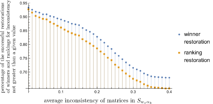
Figure 3: The ratio of number of cases where APDD managed to restore the winner (circles) or restore the entire ranking (squares) to the number of all considered cases.

In Figure 3 we can see how the ratios of WR and RR to the number of considered sets $S_{w_{x}\alpha_{k}}$ changes with the increase in the average inconsistency of $S_{w_{x}\alpha_{k}}$ in case of the APDD method. In particular, we can observe that for the average consistency $\textit{CI}\leq 0.1$, there are $89\%$ of cases (value $0.89$ on the plot) in which APDD was able to restore the correct winner. Similarly, there are $86\%$ of cases where APDD reconstructed a complete ranking.

The AID and MX methods results are presented in Figures 4 and 5, respectively.

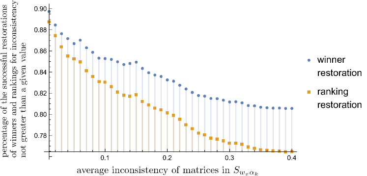
Figure 4: The ratio of number of cases where AID managed to restore the winner (circles) or restore the entire ranking (squares) to the number of all considered cases.

For $\textit{CI}\leq 0.1$, AID restored the winner in $85\%$ and the whole ranking in $83\%$. The combined MX method reconstructed the winer in $88\%$ and the complete ranking in $86\%$. In all cases, the number of decision models in which the winner was restored is slightly larger than the number of those where the entire ranking was restored.

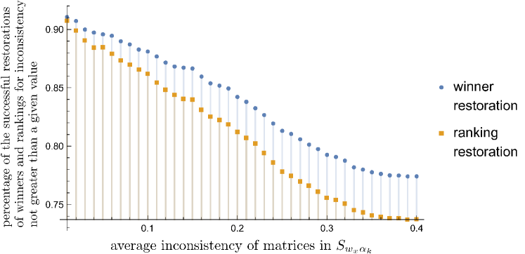
Figure 5: The ratio of number of cases where MX managed to restore the winner (circles) or restore the entire ranking (squares) to the number of all considered cases.

Despite the good efficiency in restoring the order of alternatives, the APDD, AID and MX methods are not able to ensure that the resulting ranking will be exactly the same as before the manipulation. In this case, the quality of the obtained result also depends on the average inconsistency of $S_{w_{x}\alpha_{k}}$. In Figures 6, 7 and 8 we see how the restored results differ from non-manipulated rankings expressed in the form of the average values of the Manhattan distances depending on $M_{d}(\bar{w}_{x},\widehat{w}_{x}^{*})$, where $*$ denotes the method used, e.g. APDD, AID or MX.

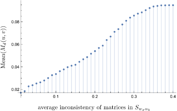
Figure 6: The average Manhattan distance $M_{d}$ between the un-manipulated ranking and its counterpart restored by the APDD method after manipulation.

Figure 7: The average Manhattan distance $M_{d}$ between the un-manipulated ranking and its counterpart restored by the AID method after manipulation.

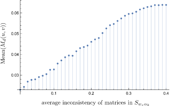
Figure 8: The average Manhattan distance $M_{d}$ between the un-manipulated ranking and its restored by the MX method after manipulation counterpart.

It can be seen that with a relatively small average inconsistency of experts (let’s say, around $0.1$), the difference between the original and the reconstructed ranking is also reasonably small. In the case of APDD it is: $M_{d}(u,v)=0.0336$, AID: $M_{d}(u,v)=0.047$ and MX $M_{d}(u,v)=0.0327$. Therefore, in a large number of cases, such a result can be considered acceptable.

4.3 Vulnerability to original ranking perturbation

In the second experiment, we assumed that all experts acted honestly. Hence, methods of aggregating expert opinions are defined to minimize the effects of manipulation one can perceive as disturbances. Therefore, our goal this time is to check to what extent the proposed methods can “disturb” the actual ranking if the manipulation did not occur. For this purpose, we took the same dataset as in the previous experiment, but this time we did not manipulate individual data sets $S_{w_{x}\alpha_{k}}$ to modify the original result. Similarly as before, $\bar{w}_{x}$ denotes the aggregated ranking (9) calculated using the standard AIP procedure (see Sec. 2.3). The results aggregated using the modified APDD, AID and MX aggregation procedures will be denoted as $\breve{w}_{x}$ with the appropriate superscripted acronym. However, this time both ranking vectors $\bar{w}_{x}$ and $\breve{w}_{x}$ are calculated based on the same data set $S_{w_{x}\alpha_{k}}$. Therefore, the distance between them can be understood as an indicator of the disturbance of the original ranking by unnecessary use of the APDD, AID and MX aggregation methods.

As expected, (Fig. 9, 10 and 11) the size of the ranking disturbances depends on the degree of inconsistency.

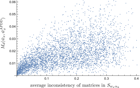
Figure 9: Distances between non-manipulated rankings calculated in a standard way $\bar{w}_{x}$ and with the help of the APDD method.

Basically, the greater the inconsistency, the greater the differences between the two vectors $\bar{w}_{x}$ and $\breve{w}_{x}$. Interestingly, the best results are achieved by the mixed method (Fig. 11), which is a combination of both other strategies (Fig. 8, 9). The advantage of the MX method can be observed not just visually. Indeed, the average distances $M_{d}\left(\bar{w}_{x},\breve{w}_{x}\right)$ between rankings aggregated using standard and modified procedures are as follows:

$$\frac{1}{4000}\sum_{\bar{w}_{x}}M_{d}\left(\bar{w}_{x},\breve{w}_{x}^{\text{APDD}}\right)=0.017$$ (10)

$$\frac{1}{4000}\sum_{\bar{w}_{x}}M_{d}\left(\bar{w}_{x},\breve{w}_{x}^{\text{AID}}\right)=0.011$$ (11)

$$\frac{1}{4000}\sum_{\bar{w}_{x}}M_{d}\left(\bar{w}_{x},\breve{w}_{x}^{\text{MX}}\right)=0.009$$ (12)

From the above, it is easy to see that, on average, the results of the MX method (value $0.009$) are the least distant from the unmodified aggregation method.

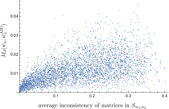
Figure 10: Distances between non-manipulated rankings calculated in a standard way $\bar{w}_{x}$ and with the help of the AID method.

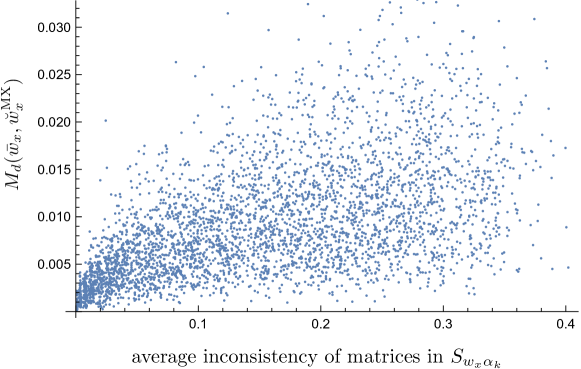
Figure 11: Distances between non-manipulated rankings calculated in a standard way $\bar{w}_{x}$ and with the help of the MX method.

The disruption of the ranking may be not only quantitative, but also qualitative. This means that the modified method may propose a ranking that will differ from the “original” with regard to the order of the alternatives. As the standard method for determining the ordinal difference between rankings is the Kendall Tau distance (3), we calculated $K_{d}(\bar{w}_{x},\breve{w}_{x})$ for every $S_{w_{x}\alpha_{k}}$ for which $I(S_{w_{x}\alpha_{k}})\leq 0.1$. The obtained values (vertical axis) can be interpreted as the expected probability that with the assumed not too high inconsistency of the group of experts ($I(S_{w_{x}\alpha_{k}})\leq 0.1$), both rankings will differ by a given number of transpositions (horizontal axis). For example, in the case of the APDD method, we can see (Fig. 12) that if the average inconsistency in the group of experts is not too high, $I(S_{w_{x}\alpha_{k}})\leq 0.1$ then there is a $92\%$ chance that both rankings remain unchanged. Going forward, there is a $2.5\%$ chance that they will differ in one transposition, etc.

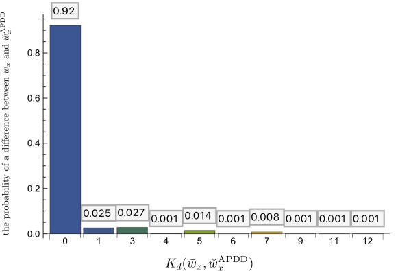
Figure 12: Estimated probability that for $I(S_{w_{x}\alpha_{k}})\leq 0.1$ the Kendall Tau distance $K_{d}(\bar{w}_{x},\breve{w}_{x}^{\text{APDD}})$ will be: $0,1,\ldots,12$.

Similarly, for the AID grouping method, the chance that the ranking will not change (i.e. $K_{d}(\bar{w}_{x},\breve{w}_{x}^{\text{AID}})=0$) is $94.4\%$ (Fig. 13). The difference of one transposition (i.e. $K_{d}(\bar{w}_{x},\breve{w}_{x}^{\text{AID}})=1$) occurred in $1.5\%$ of cases, etc.

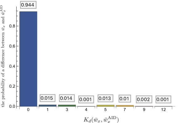
Figure 13: Estimated probability that for $I(S_{w_{x}\alpha_{k}})\leq 0.1$ the Kendall Tau distance $K_{d}(\bar{w}_{x},\breve{w}_{x}^{\text{AID}})$ will be: $0,1,\ldots,12$.

Finally, in the case of a mixed method the chance that the ranking remains unchanged (i.e. $K_{d}(\bar{w}_{x},\breve{w}_{x}^{\text{MX}})=0$) is $95.1\%$ (Fig. 14). Analogously, the difference of one transposition (i.e. $K_{d}(\bar{w}_{x},\breve{w}_{x}^{\text{MX}})=1$) occurred in $1.4\%$ of cases, three transpositions are needed to transform $\bar{w}_{x}$ into $\breve{w}_{x}^{\text{MX}}$ in $1.2\%$ of cases and so on.

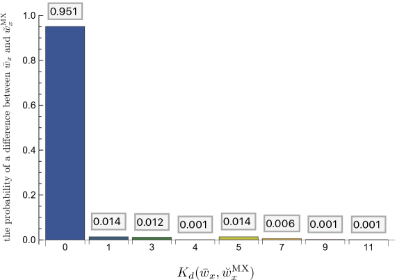
Figure 14: Estimated probability that for $I(S_{w_{x}\alpha_{k}})\leq 0.1$ the Kendall Tau distance $K_{d}(\bar{w}_{x},\breve{w}_{x}^{\text{MX}})$ will be: $0,1,\ldots,12$.

4.4 Experiments summary and discussion

The conducted experiments used $4000$ sets containing $20$ matrices, each simulating the opinions of experts in a group decision-making process. The simulated scenarios contained from $5$ to $7$ alternatives. The first of the Montecarlo experiments consisted in simulating a simple manipulation and checking the robustness of the experts’ ranking aggregation. Three proposed methods were tested: APDD (Aggregation of Preferential Distance-Driven expert prioritization), AID (Aggregation of Inconsistency-Driven expert prioritization) and MX (the mixed method, being a combination of the previous two). For all methods, their efficiency depended on the average inconsistency of the matrix in the tested 20-element set. The higher the inconsistency, the lower the effectiveness. In case of small inconsistencies (close to 0), the effectiveness of the APDD method was close to $95\%$. i.e. in $95\%$ of cases out of a hundred, this method was able to mitigate the negative effects of the attack (Fig. 3). The AID method fared slightly worse with effectiveness around $88\%$ (Fig. 4). The mixed approach seems to fall between APDD and AID, with its effectiveness around $90\%$ (Fig. 5). For inconsistency around $0.1$, the effectiveness of APDD drops to $89\%$ for WR (winner restoration) and $86\%$ for RR (ranking restoration). The results for AID and MX are respectively: $85\%$ (WR), $83\%$ (RR), $88\%$ (WR) and $86\%$ (RR). Quantitative differences between the original (non-manipulated) ranking and the “fixed” ranking were not large (Fig. 6, 7 and 8) and varied from $0.0327$ to $0.047$. Interestingly, the mixed method performed as well as the first APDD method.

The purpose of the second experiment was to test the proposed aggregation methods on non-manipulated data. In this case, these methods seem unnecessary and superfluous. Hence, changes in the differences between the ranking obtained using these methods and the ranking obtained using the classical method can be treated as an unnecessary disturbance. We examined the generated data for quantitative and qualitative differences between the two ranking vectors. We achieved the best quantitative result for the MX method, with the average Manhattan distance of $0.009$ (12). The AID method fared slightly worse with the Manhattan distance $0.011$ (11), and at the end APDD with a result of $0.017$ (10). In all of the cases, it can be seen that this distance depends on the average inconsistency of experts and increases along with increasing inconsistency.

To examine the qualitative difference between the classic aggregation method and the modified methods, we used Kendall’s tau distance measure and the subset of data for which the average inconsistency is not too high (less than $0.1$). With these assumptions, the MX method turned out to be the best again, as in $95\%$ of cases the ranking did not change (Fig. 14). The AID method fared slightly worse since for 94% of cases the order remained unchanged. The APDD method took last position with $92\%$ untouched rankings.

The proposed methods are not perfect. However, almost $90\%$ of effectiveness related to eliminating the negative effects of manipulation is achieved, with a $5\text{\textendash}8\%$ risk of introducing disturbances when the manipulation occurs. The negative impact in the second case is much less severe when the ranking result is interpreted quantitatively, i.e., when the rank value is more important than the position on the list. Then, potentially significant changes introduced by the manipulation can be elimiated or mitigated with relatively small quantitative changes in the non-manipulated ranking. However, is it worth using modified aggregation methods when the ranking result is ultimately given an ordinal meaning? It depends on the subjective assessment of the people responsible for the decision process. In other words, if the risk of manipulation is not negligible, then it may be worth using the presented aggregation methods. In the article, we proposed three heuristic ranking aggregation methods, the third of which combined the other two. Based on the conducted experiments, the third one is the most effective in practice. However, this observation suggests that adding more heuristics to identify possible manipulations could improve the results. In particular, effective methods of mitigating the effects of manipulation should simultaneously be based on many mutually complementary approaches.

5 Summary

The article presents three modified procedures for aggregating expert opinions that can be used in group decision making using the AHP method. They allow for mitigation (or elimination) of the adverse effects of manipulation with a small risk of distorting of the ranking. The first two methods are based on heuristics that make the weight of a given expert dependent on the level of its inconsistency and the group’s average opinion. The third method, perhaps the most promising, combines the other two. Developing more secure and tamper-resistant methods based on comparing alternatives in pairs will require further study of attack and defense methods against manipulation. Thus, the presented results bring us one step closer to this goal.

References

- Aczél and Saaty [1983] Aczél, J., Saaty, T.L., 1983. Procedures for synthesizing ratio judgements. Journal of Mathematical Psychology 27, 93–102. URL: http://dx.doi.org/10.1016/0022-2496(83)90028-7, doi:10.1016/0022-2496(83)90028-7.
- Aupetit and Genest [1993] Aupetit, B., Genest, C., 1993. On some useful properties of the Perron eigenvalue of a positive reciprocal matrix in the context of the analytic hierarchy process. European Journal of Operational Research , 1–6.
- Bana e Costa et al. [2016] Bana e Costa, C., De Corte, J.M., Vansnick, J., 2016. On the mathematical foundation of MACBETH, in: Figueira, J., Greco, S., Ehrgott, M. (Eds.), Multiple Criteria Decision Analysis: State of the Art Surveys. Springer Verlag, Boston, Dordrecht, London, pp. 421–463.
- Brandt et al. [2016] Brandt, F., Conitzer, V., Endriss, U., Lang, J., Procaccia, A.D. (Eds.), 2016. Handbook of Computational Social Choice. Cambridge University Press.
- Brunelli [2018] Brunelli, M., 2018. A survey of inconsistency indices for pairwise comparisons. International Journal of General Systems 47, 751–771.
- Castellan [2013] Castellan, N.J. (Ed.), 2013. Individual and group decision making: current issues. Taylor and Francis Group, Hillsdale, N.J.
- Connor [1987] Connor, W.R., 1987. Tribes, festivals and processions; civic ceremonial and political manipulation in archaic Greece. The Journal of Hellenic Studies 107, 40–50. doi:10.2307/630068.
- Crawford and Williams [1985] Crawford, R., Williams, C., 1985. A note on the analysis of subjective judgement matrices. Journal of Mathematical Psychology 29, 387 – 405.
- Dong and Saaty [2014] Dong, Q., Saaty, T.L., 2014. An analytic hierarchy process model of group consensus. Journal of Systems Science and Systems Engineering 23, 362–374. URL: http://link.springer.com/10.1007/s11518-014-5247-8, doi:10.1007/s11518-014-5247-8.
- Dong et al. [2018] Dong, Y., Liu, Y., Liang, H., Chiclana, F., Herrera-Viedma, E., 2018. Strategic weight manipulation in multiple attribute decision making. Omega 75, 154–164. doi:https://doi.org/10.1016/j.omega.2017.02.008.
- Dong and Xu [2016] Dong, Y., Xu, J., 2016. Consensus Building in Group Decision Making: Searching the Consensus Path with Minimum Adjustments. Springer. doi:10.1007/978-981-287-892-2.
- Dong et al. [2021] Dong, Y., Zha, Q., Zhang, H., Herrera, F., 2021. Consensus Reaching and Strategic Manipulation in Group Decision Making With Trust Relationships. IEEE Transactions on Systems, Man, and Cybernetics: Systems 51, 6304–6318. URL: https://ieeexplore.ieee.org/document/8957414/, doi:10.1109/TSMC.2019.2961752.
- Dyer [1990] Dyer, J.S., 1990. Remarks on the analytic hierarchy process. Management Science 36, 249–258.
- Faliszewski et al. [2010] Faliszewski, P., Hemaspaandra, E., Hemaspaandra, L.A., 2010. Using complexity to protect elections. Communications of the ACM 53, 74–82. doi:10.1145/1839676.1839696.
- Faliszewski et al. [2009] Faliszewski, P., Hemaspaandra, E., Hemaspaandra, L.A., Rothe, J., 2009. Llull and Copeland Voting Computationally Resist Bribery and Constructive Control. J. Artif. Intell. Res. (JAIR) 35, 275–341.
- Forman and Peniwati [1998] Forman, E., Peniwati, K., 1998. Aggregating individual judgments and priorities with the analytic hierarchy process. European Journal of Operational Research 108, 165–169.
- Forman [1993] Forman, E.H., 1993. Facts and fictions about the analytic hierarchy process. Mathematical and Computer Modelling 17, 19–26.
- Garcia-Zamora et al. [2022] Garcia-Zamora, D., Labella, A., Ding, W., Rodriguez, R.M., Martinez, L., 2022. Large-Scale Group Decision Making: A Systematic Review and a Critical Analysis. IEEE/CAA Journal of Automatica Sinica 9, 949–966. URL: https://ieeexplore.ieee.org/document/9785937/, doi:10.1109/JAS.2022.105617.
- Gärdenfors [1976] Gärdenfors, P., 1976. Manipulation of social choice functions. Journal of Economic Theory 13, 217–228. URL: https://linkinghub.elsevier.com/retrieve/pii/0022053176900168, doi:10.1016/0022-0531(76)90016-8.
- Gibbard [1973] Gibbard, A., 1973. Manipulation of voting schemes: A general result. Econometrica 41, 587–601. ISBN: 00129682.
- Grošelj et al. [2015] Grošelj, P., Zadnik Stirn, L., Ayrilmis, N., Kuzman, M.K., 2015. Comparison of some aggregation techniques using group analytic hierarchy process. Expert Systems with Applications 42, 2198–2204.
- Harker [1987a] Harker, P.T., 1987a. Alternative modes of questioning in the analytic hierarchy process. Mathematical Modelling 9, 353 – 360. doi:https://doi.org/10.1016/0270-0255(87)90492-1.
- Harker [1987b] Harker, P.T., 1987b. Incomplete pairwise comparisons in the analytic hierarchy process. Mathematical Modelling 9, 837–848.
- Hnatiienko [2019] Hnatiienko, H., 2019. Choice Manipulation in Multicriteria Optimization Problems, in: Proceedings of International Conference on Intelligent Tutoring Systems.
- Hoyt [1997] Hoyt, P.D., 1997. The Political Manipulation of Group Composition: Engineering the Decision Context. Political Psychology 18, 771–790. URL: https://onlinelibrary.wiley.com/doi/10.1111/0162-895X.00078, doi:10.1111/0162-895X.00078.
- Hwang and Lin [1987] Hwang, C., Lin, M., 1987. Group Decision Making under Multiple Criteria: Methods and Applications. Lecture Notes in Economics and Mathematical Systems no. 281. 1 ed., Springer.
- Kendall [1938] Kendall, M.G., 1938. A new measure of rank correlation. Biometrika 30, 81.
- Kilgour and Eden [2021] Kilgour, D.M., Eden, C., 2021. Handbook of group decision and negotiation. Springer reference. 2nd ed. ed., Springer.
- Koczkodaj [1993] Koczkodaj, W.W., 1993. A new definition of consistency of pairwise comparisons. Math. Comput. Model. 18, 79–84. URL: http://dx.doi.org/10.1016/0895-7177(93)90059-8, doi:10.1016/0895-7177(93)90059-8.
- Kułakowski [2014] Kułakowski, K., 2014. Heuristic Rating Estimation Approach to The Pairwise Comparisons Method. Fundamenta Informaticae 133, 367–386. URL: https://doi.org/10.3233/FI-2014-1081, doi:10.3233/FI-2014-1081.
- Kułakowski [2020a] Kułakowski, K., 2020a. On the geometric mean method for incomplete pairwise comparisons. Mathematics 8, 1–12.
- Kułakowski [2020b] Kułakowski, K., 2020b. Understanding the Analytic Hierarchy Process. Chapman and Hall / CRC Press. doi:10.1201/b21817.
- Kułakowski and Kedzior [2016] Kułakowski, K., Kedzior, A., 2016. Some Remarks on the Mean-Based Prioritization Methods in AHP, in: Nguyen, N.T., Iliadis, L., Manolopoulos, Y., Trawiński, B. (Eds.), Lecture Notes In Computer Science, Computational Collective Intelligence: 8th International Conference, ICCCI 2016, Halkidiki, Greece, September 28-30, 2016. Proceedings, Part I, Springer International Publishing. pp. 434–443. URL: http://dx.doi.org/10.1007/978-3-319-45243-2-40, doi:10.1007/978-3-319-45243-2-40.
- Kułakowski et al. [2019] Kułakowski, K., Szybowski, J., Prusak, A., 2019. Towards quantification of incompleteness in the pairwise comparisons methods. International Journal of Approximate Reasoning 115, 221–234.
- Kułakowski and Talaga [2020] Kułakowski, K., Talaga, D., 2020. Inconsistency indices for incomplete pairwise comparisons matrices. International Journal of General Systems 49, 174–200. URL: https://doi.org/10.1080/03081079.2020.1713116, doi:10.1080/03081079.2020.1713116.
- Lev and Lewenberg [2019] Lev, O., Lewenberg, Y., 2019. “Reverse Gerrymandering”: Manipulation in Multi-Group Decision Making. Proceedings of the AAAI Conference on Artificial Intelligence 33, 2069–2076. URL: https://ojs.aaai.org/index.php/AAAI/article/view/4037, doi:10.1609/aaai.v33i01.33012069.
- Lootsma [1999a] Lootsma, F.A. (Ed.), 1999a. Group Decision Making. Springer US, Boston, MA. pp. 139–160. URL: https://doi.org/10.1007/978-0-585-28008-06, doi:10.1007/978-0-585-28008-06.
- Lootsma [1999b] Lootsma, F.A. (Ed.), 1999b. Multi-Criteria Decision Analysis via Ratio and Difference Judgement. volume 29 of Applied Optimization. Springer US, Boston, MA. URL: http://link.springer.com/10.1007/b102374, doi:10.1007/b102374.
- Macintyre [1993] Macintyre, I.D.A., 1993. Manipulation under majority decision-making when no majority suffers and preferences are strict. Theory and Decision 35, 167–177. URL: http://link.springer.com/10.1007/BF01074957, doi:10.1007/BF01074957.
- Maoz [1990] Maoz, Z., 1990. Framing the National Interest: The Manipulation of Foreign Policy Decisions in Group Settings. World Politics 43, 77–110. URL: https://doi.org/10.2307/2010552, doi:10.2307/2010552.
- Mazurek [2023] Mazurek, J. (Ed.), 2023. Advances in Pairwise Comparisons: Detection, Evaluation and Reduction of Inconsistency. Multiple Criteria Decision Making, Springer Nature Switzerland.
- Ramanathan and Ganesh [1994] Ramanathan, R., Ganesh, L., 1994. Group preference aggregation methods employed in AHP: An evaluation and an intrinsic process for deriving members’ weightages. European Journal of Operational Research 79, 249 – 265. URL: https://doi.org/10.1016/0377-2217(94)90356-5, doi:10.1016/0377-2217(94)90356-5.
- Rezaei [2015] Rezaei, J., 2015. Best-worst multi-criteria decision-making method. Omega 53, 49–57.
- Saaty [1987] Saaty, R.W., 1987. The analytic hierarchy process — what it is and how it is used. Mathematical Modelling 9, 161–176. URL: https://doi.org/10.1016/0270-0255(87)90473-8, doi:10.1016/0270-0255(87)90473-8.
- Saaty [1977] Saaty, T.L., 1977. A scaling method for priorities in hierarchical structures. Journal of Mathematical Psychology 15, 234 – 281. doi:10.1016/0022-2496(77)90033-5.
- Saaty [1989] Saaty, T.L., 1989. Group Decision Making and the AHP. Springer Berlin Heidelberg, Berlin, Heidelberg. pp. 59–67. URL: https://doi.org/10.1007/978-3-642-50244-64, doi:10.1007/978-3-642-50244-64.
- Saaty [2008] Saaty, T.L., 2008. Relative Measurement and Its Generalization in Decision Making. Why Pairwise Comparisons are Central in Mathematics for the Measurement of Intangible Factors. The Analytic Hierarchy/Network Process. Estadística e Investigación Operativa / Statistics and Operations Research (RACSAM) 102, 251–318.
- Sasaki [2023] Sasaki, Y., 2023. Strategic manipulation in group decisions with pairwise comparisons: A game theoretical perspective. European Journal of Operational Research 304, 1133–1139. URL: https://linkinghub.elsevier.com/retrieve/pii/S0377221722003885, doi:10.1016/j.ejor.2022.05.015.
- Smith [1999] Smith, D.A., 1999. Manipulability measures of common social choice functions. Social Choice and Welfare 16, 639–661. doi:10.1007/s003550050166.
- Sun et al. [2022] Sun, Q., Wu, J., Chiclana, F., Wang, S., Herrera-Viedma, E., Yager, R.R., 2022. An approach to prevent weight manipulation by minimum adjustment and maximum entropy method in social network group decision making. Artificial Intelligence Review URL: https://link.springer.com/10.1007/s10462-022-10361-8, doi:10.1007/s10462-022-10361-8.
- Taylor [2005] Taylor, A.D., 2005. Social Choice and the Mathematics of Manipulation. Outlooks, Cambridge University Press. doi:10.1017/CBO9780511614316.
- Wu et al. [2021] Wu, J., Cao, M., Chiclana, F., Dong, Y., Herrera-Viedma, E., 2021. An Optimal Feedback Model to Prevent Manipulation Behavior in Consensus Under Social Network Group Decision Making. IEEE Transactions on Fuzzy Systems 29, 1750–1763. URL: https://ieeexplore.ieee.org/document/9057368/, doi:10.1109/TFUZZ.2020.2985331.
- Yager [2001] Yager, R.R., 2001. Penalizing strategic preference manipulation in multi-agent decision making. IEEE Transactions on Fuzzy Systems 9, 393–403. doi:10.1109/91.928736.
- Yager [2002] Yager, R.R., 2002. Defending against strategic manipulation in uninorm-based multi-agent decision making. European Journal of Operational Research 141, 217–232. doi:10.1016/S0377-2217(01)00267-3.