Subsonic flows with a contact discontinuity in a two-dimensional finitely long curved nozzle

Abstract

This paper concerns the structural stability of subsonic flows with a contact discontinuity in a two-dimensional finitely long slightly curved nozzle. We establish the existence and uniqueness of subsonic flows with a contact discontinuity by prescribing the entropy function, the Bernoulli quantity and the horizontal mass flux distribution at the entrance and the flow angle at the exit. The problem can be formulated as a free boundary problem for the hyperbolic-elliptic coupled system. To deal with the free boundary value problem, the Lagrangian transformation is employed to straighten the contact discontinuity. The Euler system is reduced to a nonlinear second-order equation for the stream function. Inspired by [4], we use the implicit function theorem to locate the contact discontinuity. We also need to develop an iteration scheme to solve a nonlinear elliptic boundary value problem with nonlinear boundary conditions in a weighted Hölder space.

Mathematics Subject Classifications 2010: 35L65, 35L67, 76H05, 76N15.

Key words: steady Euler system, contact discontinuity, free boundary, structural stability, Lagrangian transformation.

1 Introduction

In this paper, we are concerned with the structural stability of subsonic flows with a contact discontinuity governed by the two-dimensional steady full Euler system in a finitely long slightly curved nozzle. The two-dimensional steady full Euler system for compressible inviscid gas is of the following form:

$$\begin{cases}{\partial}_{x_{1}}(\rho u_{1})+{\partial}_{x_{2}}(\rho u_{2})=0,\\ {\partial}_{x_{1}}(\rho u_{1}^{2})+{\partial}_{x_{2}}(\rho u_{1}u_{2})+{\partial}_{x_{1}}P=0,\\ {\partial}_{x_{1}}(\rho u_{1}u_{2})+{\partial}_{x_{2}}(\rho u_{2}^{2})+{\partial}_{x_{2}}P=0,\\ {\partial}_{x_{1}}(\rho u_{1}E+u_{1}P)+{\partial}_{x_{2}}(\rho u_{2}E+u_{2}P)=0,\\ \end{cases}$$ (1.1)

where $\bm{u}=(u_{1},u_{2})$ is the velocity, $\rho$ is the density, $P$ is the pressure, $E$ is the energy, respectively. For polytropic gas, $P=A(S)\rho^{\gamma}$, where $A(S)=Re^{S}$ and $\gamma\in(1,+\infty)$, $R$ are positive constants. Denote the Bernoulli’s function and the local sonic speed by $B=\frac{1}{2}|{\textbf{u}}|^{2}+\frac{\gamma P}{(\gamma-1)\rho}$ and $c(\rho,A)=\sqrt{A\gamma}\rho^{\frac{\gamma-1}{2}}$, respectively. Then the system (1.1) is hyperbolic for supersonic flows ($|\textbf{u}|>c(\rho,A)$), and hyperbolic-elliptic coupled for subsonic flows ($|\textbf{u}|<c(\rho,A)$).

To understand conditions on the contact discontinuity curve, we introduce the notation of weak solution of the full Euler system (1.1). Suppose that a domain $\mathcal{D}$ in $\mathbb{R}^{2}$ is divided by a $C^{1}$-curve $\Gamma$ into sub-domains $\mathcal{D}^{+}$ and $\mathcal{D}^{-}$ such that $\mathcal{D}=\mathcal{D}^{-}\cup\Gamma\cup\mathcal{D}^{+}$. Assume that $\bm{U}=(\rho,u_{1},u_{2},P)$ is a $C^{1}$ solution of Euler equation (1.1) in each domain $\mathcal{D}^{+}$ and $\mathcal{D}^{-}$ and is continuous up to the boundary $\Gamma$ in each sub-domain. If $\bm{U}$ is a weak solution for (1.1) in domain $\mathcal{D}$, by using integration by parts, we see that the following Rankine-Hugoniot conditions hold along $\Gamma$ almost everywhere:

$$\begin{cases}n_{1}[\rho u_{1}]+n_{2}[\rho u_{2}]=0,\\ n_{1}[\rho u_{1}^{2}]+n_{1}[P]+n_{2}[\rho u_{1}u_{2}]=0,\\ n_{1}[\rho u_{1}u_{2}]+n_{2}[\rho u_{2}^{2}]+n_{2}[P]=0,\\ n_{1}[\rho u_{1}(E+\frac{P}{\rho})]+n_{2}[\rho u_{2}(E+\frac{P}{\rho})]=0,\\ \end{cases}$$ (1.2)

where $\mathbf{n}=(n_{1},n_{2})$ is the unit normal vector to $\Gamma$, and $[F](\mathbf{x})=F_{+}(\mathbf{x})-F_{-}(\mathbf{x})$ denotes the jump across the curve $\Gamma$ for a piecewise smooth function $F$.

Let $\bm{\tau}=(\tau_{1},\tau_{2})$ as the unit tangential vector to $\Gamma$, which means that $\mathbf{n}\cdot{\bm{\tau}}=0$. Taking the dot product of $(\eqref{1-2}_{2},\eqref{1-2}_{3})$ with $\mathbf{n}$ and $\bm{\tau}$ respectively, we have

$$\rho(\mathbf{u}\cdot\mathbf{n})[\mathbf{u}\cdot\bm{\tau}]_{\Gamma}=0,\quad[\rho(\mathbf{u}\cdot\mathbf{n})^{2}+P]_{\Gamma}=0.$$ (1.3)

Assume that $\rho>0$ in $\bar{\mathcal{D}}$, (1.3) implies either $\mathbf{u}\cdot\mathbf{n}=0$ on $\Gamma$ or $[\mathbf{u}\cdot\bm{\tau}]_{\Gamma}=0$. If $\mathbf{u}\cdot\mathbf{n}\neq 0$ and $[\mathbf{u}\cdot\bm{\tau}]_{\Gamma}=0$ hold on $\Gamma$, the curve $\Gamma$ is called a shock; if the flow moves along both sides of $\Gamma$ such that $\mathbf{u}\cdot\mathbf{n}=0$ on $\Gamma$, the curve $\Gamma$ is called a contact discontinuity. In the latter case, $\mathbf{u}\cdot\mathbf{n}=0$ and the second equation in(1.3) give $[P]=0$. Then we get the R-H conditions corresponding to a contact discontinuity as follows:

$$\mathbf{u}\cdot\mathbf{n}=0\quad{\rm{and}}\quad[P]=0\quad{\rm{on}}\ \Gamma.$$ (1.4)

Admissible shocks, centered rarefaction waves and contact discontinuities are fundamental wave patterns in quasi-linear hyperbolic conservation laws. The stability analysis of these elementary waves is very important both in physics and mathematics. In the book [11], Courant and Friedrichs had presented some nonlinear phenomenas for steady compressible flows, such as Mach reflection, jet flows, and their interactions. All these phenomenas are formulated by elementary waves including contact discontinuities. So to understand the stability of contact discontinuity is an important step in studying these phenomenas.

In recently years, there have been many interesting results on contact discontinuity problems for various physically situations. The stability of contact discontinuity for subsonic flows in infinite nozzles was established in [1] and [2, 3] with a Helmholtz decomposition. The global existence and uniqueness of the subsonic contact discontinuity with large vorticity in infinity long nozzles were obtained in [7] by the theory of compensated compactness, which is not a perturbation around piecewise constant solutions. The stability of supersonic flat contact discontinuity and transonic flat contact discontinuity for 2-D steady Euler flows in a finite nozzle was established in [13, 14]. The stability of two-dimensional transonic contact discontinuity over a solid wedge and three-dimensional supersonic and transonic contact discontinuity were established in [5, 6] and [18, 19, 20]. The contact discontinuity in the Mach reflection was also studied in [9, 10]. Recently, the existence, uniqueness and stability of subsonic flows past an airfoil with a vortex line were established in [4]. The well-posedness theory for the steady subsonic jet flow with a shock and a contact discontinuity was established in [16].

In this paper, we study the structural stability of subsonic flows with a contact discontinuity in a two-dimensional finitely long slightly curved nozzle. The contact discontinuity is part of the solution and is unknown, thus this is a free boundary that separates the subsonic flow in the upper and lower layers of the nozzle. Thanks to the fundamental feature of the contact discontinuity, namely, the tangent of the contact discontinuity is parallel to the velocity of the flow on its both sides, we can employ the Lagrangian transformation to straighten the free boundary. Then by introducing a stream function and solving the hyperbolic equations for the entropy and the Bernoulli’s function, the Euler system can be reduced to a nonlinear second-order equation for the stream function in upper and lower domains, respectively. Then we can develop an iteration scheme to solve a nonlinear elliptic boundary value problem with nonlinear boundary conditions in a weighted Hölder space.

The other key ingredient in our mathematical analysis is to use the implicit function theorem to locate the contact discontinuity. This idea is motivated by the discussion of airfoil problem in [4]. For the problem of subsonic flows past an airfoil with a vortex line at the trailing edge, the vortex line attached to the trailing edge is a contact discontinuity and is treated as a free boundary, the authors employed the implicit function theorem to solve this problem. In this paper, we modified the approach in [4] to study our problem of subsonic flows with a contact discontinuity in a two-dimensional finitely long curved nozzle. We choose a suitable weighted H$\ddot{\rm{o}}$lder space and design a proper map to verify the conditions in the implicit function theorem. Then we can locate the contact discontinuity by the implicit function theorem. The detailed analysis will be given in Section 5.

This paper will be arranged as follows. In Section 2, we formulate the problem of subsonic flows with a contact discontinuity in a two-dimensional finitely long curved nozzle and state the main result. In Section 3, we first employ the Lagrangian transformation to straighten the contact discontinuity. Then by introducing a stream function and solving the hyperbolic equations for the entropy and the Bernoulli’s function, the Euler system can be reduced to a nonlinear second-order equation for the stream function in upper and lower domains, respectively. Finally, we state the implicit function theorem and the main steps to solve the free boundary problem 3.1. In Section 4, we first linearize the nonlinear equation and solve the linear equation in a suitable weighted H$\ddot{\rm{o}}$lder space. Then the framework of the contraction mapping theorem can be used to find the solution of the nonlinear equation. In Section 5, we choose a suitable weighted H$\ddot{\rm{o}}$lder space and design a proper map to verify the conditions in the implicit function theorem. Then by using the implicit function theorem, we locate the contact discontinuity. In Section 6, we finish the proof of the main theorem.

2 Mathematical problem and the main result

In this section, we give a detailed formulation of subsonic flows with a contact discontinuity in a two-dimensional finitely long curved nozzle and state the main result. First, we consider a special class of subsonic flows with a straight contact discontinuity in a finitely long flat nozzle.

The flat nozzle (Fig 1) of the length $L$ can be described by

$$\Omega_{b}=\{(x_{1},x_{2}):0<x_{1}<L,\ -1<x_{2}<1\}.$$

Fig 1: Subsonic flows with a contact discontinuity in a finitely long flat nozzle

Consider two layers of steady smooth Euler flows separated by the line $x_{2}=0$ satisfying the following properties:

1. The velocity and density of the top and bottom layers are given by $(u_{b}^{+},0),\rho_{b}^{+}$ and $(u_{b}^{-},0),\rho_{b}^{-}$, where $u_{b}^{\pm}>0$ and $\rho_{b}^{\pm}>0$;

2. the pressure of both the top and bottom layers are given by the same positive constant $P_{b}$;

3. the flow in the top and bottom layers are subsonic, i.e.,

   $$(u_{b}^{\pm})^{2}<\frac{\gamma P_{b}}{\rho_{b}^{\pm}}.$$

Then

$$\bm{U}_{b}=\begin{cases}\bm{U}_{b}^{+}:=(\rho_{b}^{+},u_{b}^{+},0,P_{b}),\quad{\rm{for}}\quad(x_{1},x_{2})\in(0,L)\times(0,1),\\ \bm{U}_{b}^{-}:=(\rho_{b}^{-},u_{b}^{-},0,P_{b}),\quad{\rm{for}}\quad(x_{1},x_{2})\in(0,L)\times(-1,0),\\ \end{cases}$$ (2.1)

is a weak solution of the steady Euler system (1.1) with a contact discontinuity on the line $x_{2}=0$, which will be called the background solution in this paper. This paper is going to establish the structural stability of this background solution under the perturbations of suitable boundary conditions on the entrance and exit and the upper and lower nozzle walls.

The two-dimensional finitely long curved nozzle $\Omega$ (Fig 2) is described by

$$\Omega=\{(x_{1},x_{2}):0<x_{1}<L,g^{-}(x_{1})<x_{2}<g^{+}(x_{1})\},$$ (2.2)

with

$$g^{\pm}(x_{1})\in C^{2,\alpha}([0,L])\quad{\rm{and}}\quad g^{\pm}(0)=\pm 1.$$

The upper and lower boundaries of the nozzle are denoted by $\Gamma_{w}^{+}$ and $\Gamma_{w}^{-}$, i.e;

$$\Gamma_{w}^{\pm}:=\{(x_{1},x_{2}):0<x_{1}<L,\ x_{2}=g^{\pm}(x_{1})\}.$$ (2.3)

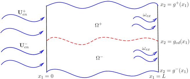
Fig 2: Subsonic flows with a contact discontinuity in a finitely long curved nozzle

The exit of the nozzle is denoted by

$$\Gamma_{L}:=\{(x_{1},x_{2}):x_{1}=L,\ g^{-}(L)<x_{2}<g^{+}(L)\}.$$ (2.4)

The entrance of the nozzle is separated into two parts:

$$\Gamma_{0}^{+}:=\{(x_{1},x_{2}):x_{1}=0,\ 0<x_{2}<1\},\quad\Gamma_{0}^{-}:=\{(x_{1},x_{2}):x_{1}=0,\ -1<x_{2}<0\}.$$ (2.5)

At the entrance $\Gamma_{0}^{\pm}$, we prescribe the boundary data for the entropy function $A$, the Bernoulli quantity $B$ and the horizontal mass distribution $J=\rho u_{1}$:

$$(A,B,J)(0,x_{2})=\begin{cases}\bm{U}_{en}^{+}(x_{2}):=(A_{en}^{+},B_{en}^{+},J_{en}^{+})(x_{2}),\quad{\rm{on}}\quad\Gamma_{0}^{+},\\ \bm{U}_{en}^{-}(x_{2}):=(A_{en}^{-},B_{en}^{-},J_{en}^{-})(x_{2}),\quad{\rm{on}}\quad\Gamma_{0}^{-}.\end{cases}$$ (2.6)

At the exit, the flow angle $\omega=\frac{u_{2}}{u_{1}}$ is prescribed by

$$\omega(L,x_{2})=\omega_{ex}(x_{2}),\quad{\rm{on}}\quad\Gamma_{L}.$$ (2.7)

Here $(\bm{U}_{en}^{+},\bm{U}_{en}^{-})(x_{2})\in\left(C^{1,\alpha}([0,1])\right)^{3}\times\left(C^{1,\alpha}([-1,0])\right)^{3}$ and $\omega_{ex}(x_{2})\in C^{2,\alpha}([g^{-}(L),g^{+}(L)])$ are close to the background solution in some sense that will be described later.

We expect the flow in the nozzle will be separated by a contact discontinuity $\Gamma:=\{x_{2}=g_{cd}(x_{1}),0<x_{1}<L\}$ with $g_{cd}(0)=0$, and we denote

$$\Omega^{+}:=\Omega\cap\{g_{cd}(x_{1})<x_{2}<g^{+}(x_{1})\},\ \Omega^{-}:=\Omega\cap\{g^{-}(x_{1})<x_{2}<g_{cd}(x_{1})\}.$$

Let

$${\bm{U}}(x_{1},x_{2})=\begin{cases}{\bm{U}}^{+}(x_{1},x_{2}):=(\rho^{+},u_{1}^{+},u_{2}^{+},P^{+})(x_{1},x_{2})\quad{\rm{in}}\quad\Omega^{+},\\ {\bm{U}}^{-}(x_{1},x_{2}):=(\rho^{-},u_{1}^{-},u_{2}^{-},P^{-})(x_{1},x_{2})\quad{\rm{in}}\quad\Omega^{-}.\\ \end{cases}$$ (2.8)

Along the contact discontinuity $x_{2}=g_{cd}(x_{1})$, the following Rankine-Hugoniot conditions hold:

$$\frac{u_{2}^{+}}{u_{1}^{+}}=\frac{u_{2}^{-}}{u_{1}^{-}}=g_{cd}^{\prime}(x_{1}),\quad P^{+}=P^{-},\quad{\rm{on}}\quad\Gamma.$$ (2.9)

On the nozzle walls $\Gamma_{w}^{+}$ and $\Gamma_{w}^{-}$, the usual slip boundary condition is imposed:

$$\frac{u_{2}^{+}}{u_{1}^{+}}=(g^{+})^{\prime}(x_{1}),\ {\rm{on}}\ \Gamma_{w}^{+},\quad\frac{u_{2}^{-}}{u_{1}^{-}}=(g^{-})^{\prime}(x_{1}),\ {\rm{on}}\ \Gamma_{w}^{-}.$$ (2.10)

In summary, we will investigate the following problem:

Problem 2.1.

Given functions $(A_{en}^{\pm},B_{en}^{\pm},J_{en}^{\pm})(x_{2})$ at the entrance and function $\omega_{ex}(x_{2})$ at the exit, find a unique piecewise smooth subsonic solution $(\bm{U}^{+},\bm{U}^{-})$ defined on $\Omega^{+}$ and $\Omega^{-}$ respectively, with the contact discontinuity $\Gamma:x_{2}=g_{cd}(x_{1})$ satisfying the Euler system (1.1) in the sense of weak solution and the Rankine-Hugoniot conditions in (2.9) and the slip boundary conditions in (2.10).

The main theorem of this paper can be stated as follows.

Theorem 2.2.

Let $\bm{U}_{0}^{\pm}=(A_{b}^{\pm},B_{b}^{\pm},J_{b}^{\pm})$, where

$$A_{b}^{\pm}=\frac{P_{b}}{(\rho_{b}^{\pm})^{\gamma}},\quad B_{b}^{\pm}=\frac{1}{2}|u_{b}^{\pm}|^{2}+\frac{\gamma P_{b}}{(\gamma-1)\rho_{b}^{\pm}},\quad J_{b}^{\pm}=\rho_{b}^{\pm}u_{b}^{\pm}.$$

Then given functions $(A_{en}^{\pm},B_{en}^{\pm},J_{en}^{\pm},\omega_{ex})$, we define

$$\sigma(\bm{U}_{en}^{+},\bm{U}_{en}^{-},\omega_{ex},g^{+},g^{-}): =\|\bm{U}_{en}^{+}-\bm{U}_{0}^{+}\|_{1,\alpha;[0,1]}+\|\bm{U}_{en}^{-}-\bm{U}_{0}^{-}\|_{1,\alpha;[-1,0]}$$ (2.11)

$$\quad+\|\omega_{ex}\|_{2,\alpha;[g^{-}(L),g^{+}(L)]}+\|g^{+}-1\|_{2,\alpha;[0,L]}$$

$$\quad+\|g^{-}+1\|_{2,\alpha;[0,L]}.$$

There exist positive constants $\sigma_{cd}$ and $\mathcal{C}$ depending only on $(A_{b}^{\pm},B_{b}^{\pm},J_{b}^{\pm},L,\alpha)$ such that if

$$\sigma(\bm{U}_{en}^{+},\bm{U}_{en}^{-},\omega_{ex},g^{+},g^{-})\leq\sigma_{cd},$$ (2.12)

Problem 2.1 has a unique piecewise smooth subsonic flow $(\bm{U}^{+},\bm{U}^{-})$ with the contact discontinuity $\Gamma:x_{2}=g_{cd}(x_{1})$ satisfying the following properties:

1. The piecewise smooth subsonic flow $(\bm{U}^{+},\bm{U}^{-})\in(C^{1,\alpha}(\Omega^{+})\cap C^{\alpha}(\overline{\Omega^{+}}))\times(C^{1,\alpha}(\Omega^{-})\cap C^{\alpha}(\overline{\Omega^{-}}))$ satisfies the following estimate:

   $$\|\bm{U}^{+}-\bm{U}_{b}^{+}\|_{C^{\alpha}(\overline{\Omega^{+}})}+\|\bm{U}^{-}-\bm{U}_{b}^{-}\|_{C^{\alpha}(\overline{\Omega^{-}})}\leq\mathcal{C}\sigma(\bm{U}_{en}^{+},\bm{U}_{en}^{-},\omega_{ex},g^{+},g^{-}).$$ (2.13)

2. The contact discontinuity curve $g_{cd}(x_{1})\in C^{2,\alpha}\left((0,L)\right)\cap C^{1,\alpha}([0,L])$ satisfies $g_{cd}(0)=0$. Furthermore, it holds that

   $$\|g_{cd}\|_{1,\alpha;[0,L]}\leq\mathcal{C}\sigma(\bm{U}_{en}^{+},\bm{U}_{en}^{-},\omega_{ex},g^{+},g^{-}).$$ (2.14)

3 The reformulation of Problem 2.1

In this section, we first employ the Lagrangian transformation to straighten the contact discontinuity, and reformulate the free boundary value problem 2.1. Then by introducing a stream function and solving the hyperbolic equations for the entropy and the Bernoulli’s function, the Euler system can be reduced to a nonlinear second-order equation for the stream function in upper and lower domains, respectively. Furthermore, all the boundary conditions at the entrance, the nozzle walls and the exit become local. Finally, we state the implicit function theorem and the main steps to solve the free boundary problem 3.1.

3.1 Reformulation by the Lagrangian transformation

To overcome the difficulty of the free boundary $\Gamma$, we will apply the Lagrangian transformation to straighten the contact discontinuity.

Let $(\bm{U}^{+}(x_{1},x_{2}),\bm{U}^{-}(x_{1},x_{2}),g_{cd}(x_{1}))$ be a solution to Problem 2.1. Define

$$m^{-}=\int_{-1}^{0}J_{en}^{-}(s){\mathrm{d}}s\quad{\rm{and}}\quad m^{+}=\int_{0}^{1}J_{en}^{+}(s){\mathrm{d}}s.$$ (3.1)

Then for any $x_{1}\in(0,L)$, it follows from the conservation of mass equation in (1.1) that

$$\int_{g^{-}(x_{1})}^{g_{cd}(x_{1})}\rho^{-}u_{1}^{-}(x_{1},s){\mathrm{d}}s=m^{-},\quad\int_{g_{cd}(x_{1})}^{g^{+}(x_{1})}\rho^{+}u_{1}^{+}(x_{1},s){\mathrm{d}}s=m^{+}.$$ (3.2)

Let

$$y_{2}(x_{1},x_{2})=\int_{g_{cd}(x_{1})}^{x_{2}}\rho u_{1}(x_{1},s){\mathrm{d}}s.$$ (3.3)

It is easy to verify that

$$\frac{{\partial}y_{2}}{{\partial}x_{1}}=-\rho u_{2},\quad\frac{{\partial}y_{2}}{{\partial}x_{2}}=\rho u_{1}.$$

Thus we can introduce the Lagrangian transformation as

$$\begin{cases}y_{1}=x_{1},\\ y_{2}=y_{2}(x_{1},x_{2}).\\ \end{cases}$$ (3.4)

A direct computation gives

$$\frac{{\partial}(y_{1},y_{2})}{{\partial}(x_{1},x_{2})}=\left|\begin{matrix}1&0\\ -\rho u_{2}&\rho u_{1}\end{matrix}\right|=\rho u_{1}.$$

So if $(\rho^{\pm},u_{1}^{\pm},u_{2}^{\pm},P^{\pm})$ are close to the background solution $(\rho_{b}^{\pm},u_{b}^{\pm},0,P_{b})$, we have $\rho^{\pm}u_{1}^{\pm}\geq\mathcal{C}_{b}>0$, where $\mathcal{C}_{b}$ depends only on the background solution. Hence the Lagrangian transformation is invertible.

Under this transformation, the domain $\Omega$ becomes

$$\mathcal{N}=\{(y_{1},y_{2}):0<y_{1}<L,\ -m^{-}<y_{2}<m^{+}\}.$$

The lower wall $\Gamma_{w}^{-}$ and upper wall $\Gamma_{w}^{+}$ of the nozzle are transformed into

$$\Sigma_{w}^{-}:=\{(y_{1},y_{2}):0<y_{1}<L,\ y_{2}=-m^{-}\},\quad\Sigma_{w}^{+}:=\{(y_{1},y_{2}):0<y_{1}<L,\ y_{2}=m^{+}\}.$$

Moreover, on $\Gamma$, we have

$$y_{2}(x_{1},g_{cd}(x_{1}))=\int_{g_{cd}(x_{1})}^{g_{cd}(x_{1})}\rho u_{1}(x_{1},s){\mathrm{d}}s=0.$$

Hence the free boundary $\Gamma$ becomes the following straight line:

$$\Sigma=\{(y_{1},y_{2}):0<y_{1}<L,\ y_{2}=0\}.$$ (3.5)

Define

$$\mathcal{N}^{-}:=\mathcal{N}\cap\{-m^{-}<y_{2}<0\},\quad\mathcal{N}^{+}:=\mathcal{N}\cap\{0<y_{2}<m^{+}\}.$$ (3.6)

Then the entrance and exit of $\mathcal{N}^{\pm}$ are defined as

$$\Sigma_{0}^{+}:=\{(y_{1},y_{2}):y_{1}=0,\ 0<y_{2}<m^{+}\},\quad\Sigma_{0}^{-}:=\{(y_{1},y_{2}):y_{1}=0,\ -m^{-}<y_{2}<0\},$$

and

$$\Sigma_{L}^{+}:=\{(y_{1},y_{2}):y_{1}=L,\ 0<y_{2}<m^{+}\},\quad\Sigma_{L}^{-}:=\{(y_{1},y_{2}):y_{1}=L,\ -m^{-}<y_{2}<0\}.$$

Let

$${\bm{U}}(y_{1},y_{2})=\begin{cases}{\bm{U}}^{+}(y_{1},y_{2}):=(\rho^{+},u_{1}^{+},u_{2}^{+},P^{+})(\mathbf{x}(y_{1},y_{2}))\quad{\rm{in}}\quad\mathcal{N}^{+},\\ {\bm{U}}^{-}(y_{1},y_{2}):=(\rho^{-},u_{1}^{-},u_{2}^{-},P^{-})(\mathbf{x}(y_{1},y_{2}))\quad{\rm{in}}\quad\mathcal{N}^{-}.\\ \end{cases}$$

Then the system (1.1) in the new coordinates can be rewritten as

$$\begin{cases}{\partial}_{y_{1}}\left(\frac{1}{\rho u_{1}}\right)-{\partial}_{y_{2}}\left(\frac{u_{2}}{u_{1}}\right)=0,\\ {\partial}_{y_{1}}u_{2}+{\partial}_{y_{2}}P=0,\\ {\partial}_{y_{1}}u_{1}+\frac{1}{\rho u_{1}}({\partial}_{y_{1}}-\rho u_{2}{\partial}_{y_{2}})P=0,\\ {\partial}_{y_{1}}A=0.\\ \end{cases}$$ (3.7)

The background solution in the Lagrange coordinates is

$${\bm{U}}_{b}=\begin{cases}{\bm{U}}_{b}^{+}:=(\rho_{b}^{+},u_{b}^{+},0,P_{b}),\quad{\rm{in}}\quad\mathcal{N}_{b}^{+},\\ {\bm{U}}_{b}^{-}:=(\rho_{b}^{-},u_{b}^{-},0,P_{b}),\quad{\rm{in}}\quad\mathcal{N}_{b}^{-},\\ \end{cases}$$ (3.8)

where

$$\mathcal{N}_{b}^{+}:=\{(y_{1},y_{2}):0<y_{1}<L,\ 0<y_{2}<m_{b}^{+}\},\quad\mathcal{N}_{b}^{-}:=\{(y_{1},y_{2}):0<y_{1}<L,\ -m_{b}^{-}<y_{2}<0\},$$

and $m_{b}^{\pm}=\rho_{b}^{\pm}u_{b}^{\pm}$. Without loss of generality, we assume that $m_{b}^{\pm}=m^{\pm}$.

In the new coordinates, the boundary data (2.6) at the entrance is given by

$${\bm{U}}_{en}(y_{2})=\begin{cases}{\bm{U}}_{en}^{+}(y_{2})=(\tilde{A}_{en}^{+},\tilde{B}_{en}^{+},\tilde{J}_{en}^{+})(y_{2}),\quad{\rm{on}}\quad\Sigma_{0}^{+},\\ {\bm{U}}_{en}^{-}(y_{2})=(\tilde{A}_{en}^{-},\tilde{B}_{en}^{-},\tilde{J}_{en}^{-})(y_{2}),\quad{\rm{on}}\quad\Sigma_{0}^{-},\\ \end{cases}$$ (3.9)

where

$$(\tilde{A}_{en}^{+},\tilde{B}_{en}^{+},\tilde{J}_{en}^{+})(y_{2})=(A_{en}^{+},B_{en}^{+},J_{en}^{+})\left(\int_{0}^{y_{2}}\frac{1}{J_{en}^{+}}(s){\mathrm{d}}s\right),$$

and

$$(\tilde{A}_{en}^{-},\tilde{B}_{en}^{-},\tilde{J}_{en}^{-})(y_{2})=(A_{en}^{-},B_{en}^{-},J_{en}^{-})\left(-\int_{y_{2}}^{0}\frac{1}{J_{en}^{-}}(s){\mathrm{d}}s\right).$$

The boundary condition (2.7) at the exit become

$$\omega(L,y_{2})=\begin{cases}\omega_{ex}(x_{2}^{+}(L,y_{2})),\quad{\rm{on}}\quad\Sigma_{L}^{+},\\ \omega_{ex}(x_{2}^{-}(L,y_{2})),\quad{\rm{on}}\quad\Sigma_{L}^{-},\\ \end{cases}$$ (3.10)

where

$$x_{2}^{+}(L,y_{2})=g_{cd}(L)+\int_{0}^{y_{2}}\frac{1}{\rho^{+}u_{1}^{+}}(L,s){\mathrm{d}}s,\quad x_{2}^{-}(L,y_{2})=g_{cd}(L)-\int_{y_{2}}^{0}\frac{1}{\rho^{-}u_{1}^{-}}(L,s){\mathrm{d}}s.$$

Hence it should be emphasized that the flow angle at the exit becomes non-local and nonlinear in the Lagrange coordinates.

The Rankine-Hugoniot conditions in (2.9) can be rewritten

$$\frac{u_{2}^{+}(y_{1},0)}{u_{1}^{+}(y_{1},0)}=\frac{u_{2}^{-}(y_{1},0)}{u_{1}^{-}(y_{1},0)}=g_{cd}^{\prime}(y_{1}),$$ (3.11)

and

$$P^{+}(y_{1},0)=P^{-}(y_{1},0).$$ (3.12)

The slip boundary conditions in (2.10) become

$$\frac{u_{2}^{+}}{u_{1}^{+}}(y_{1},m^{+})=(g^{+})^{\prime}(y_{1}),\ {\rm{on}}\ \Sigma_{w}^{+},\quad\frac{u_{2}^{-}}{u_{1}^{-}}(y_{1},-m^{-})=(g^{-})^{\prime}(y_{1}),\ {\rm{on}}\ \Sigma_{w}^{-}.$$ (3.13)

3.2 Reduction of the Euler system

In this subsection, we introduce a stream function to reformulate the Euler system (3.7) as a nonlinear second-order equation with suitable boundary conditions.

By the first equation in (3.7), one can introduce a stream function

$$\varphi(y_{1},y_{2})=\begin{cases}\varphi^{-}(y_{1},y_{2}),\quad{\rm{for}}\quad(y_{1},y_{2})\in\mathcal{N}^{-},\\ \varphi^{+}(y_{1},y_{2}),\quad{\rm{for}}\quad(y_{1},y_{2})\in\mathcal{N}^{+},\\ \end{cases}$$ (3.14)

such that

$${\partial}_{y_{1}}\varphi=\frac{u_{2}}{u_{1}},\quad{\partial}_{y_{2}}\varphi=\frac{1}{\rho u_{1}},\quad\varphi(0,0)=0.$$ (3.15)

That is

$$u_{1}=\frac{1}{\rho{\partial}_{y_{2}}\varphi},\quad u_{2}=\frac{{\partial}_{y_{1}}\varphi}{\rho{\partial}_{y_{2}}\varphi}.$$

It follows from the fourth equation in (3.7) that one has

$$A=\tilde{A}_{en}(y_{2}).$$ (3.16)

Moreover, the Bernoulli’s function $B$ in the Lagrangian coordinates satisfies

$${\partial}_{y_{1}}B=0.$$

Thus the following equation holds:

$$\frac{1}{2}\left(\frac{1}{(\rho{\partial}_{y_{2}}\varphi)^{2}}+\frac{({\partial}_{y_{1}}\varphi)^{2}}{(\rho{\partial}_{y_{2}}\varphi)^{2}}\right)+\frac{\tilde{A}_{en}\gamma\rho^{\gamma-1}}{\gamma-1}=\tilde{B}_{en}(y_{2}).$$ (3.17)

Define

$$\mathcal{B}(\rho,\nabla\varphi,\tilde{A}_{en},\tilde{B}_{en})=\frac{1+({\partial}_{y_{1}}\varphi)^{2}}{2({\partial}_{y_{2}}\varphi)^{2}}+\frac{\tilde{A}_{en}\gamma\rho^{\gamma+1}}{\gamma-1}-\tilde{B}_{en}\rho^{2}.$$

Since the flow is subsonic, we have

$$\frac{{\partial}}{{\partial}\rho}\mathcal{B}(\rho,\nabla\varphi,\tilde{A}_{en},\tilde{B}_{en})=\rho(c^{2}(\rho,\tilde{A}_{en})-u_{1}^{2}-u_{2}^{2})>0.$$

Hence the implicit function theorem implies that $\rho$ can be expressed as a function of $\nabla\varphi,\tilde{A}_{en},\tilde{B}_{en}$, namely, $\rho=\rho(\nabla\varphi,\tilde{A}_{en},\tilde{B}_{en})$. Moreover, a direct computation yields that

$$\frac{{\partial}\rho}{{\partial}({\partial}_{y_{1}}\varphi)} =-\frac{{\partial}_{y_{1}}\varphi}{\rho({\partial}_{y_{2}}\varphi)^{2}\left(c^{2}(\rho,\tilde{A}_{en})-\frac{1+({\partial}_{y_{1}}\varphi)^{2}}{(\rho{\partial}_{y_{2}}\varphi)^{2}}\right)},$$

$$\frac{{\partial}\rho}{{\partial}({\partial}_{y_{2}}\varphi)} =\frac{1+({\partial}_{y_{1}}\varphi)^{2}}{\rho({\partial}_{y_{2}}\varphi)^{3}\left(c^{2}(\rho,\tilde{A}_{en})-\frac{1+({\partial}_{y_{1}}\varphi)^{2}}{(\rho{\partial}_{y_{2}}\varphi)^{2}}\right)},$$

$$\frac{{\partial}\rho}{{\partial}\tilde{A}_{en}} =-\frac{\gamma\rho^{\gamma}}{(\gamma-1)\left(c^{2}(\rho,\tilde{A}_{en})-\frac{1+({\partial}_{y_{1}}\varphi)^{2}}{(\rho{\partial}_{y_{2}}\varphi)^{2}}\right)},$$

$$\frac{{\partial}\rho}{{\partial}\tilde{B}_{en}} =\frac{\rho}{c^{2}(\rho,\tilde{A}_{en})-\frac{1+({\partial}_{y_{1}}\varphi)^{2}}{(\rho{\partial}_{y_{2}}\varphi)^{2}}}.$$

Thus, the solution $\bm{U}$ can be expressed as a vector-value function of $\varphi,\tilde{A}_{en},\tilde{B}_{en}$:

$$\bm{U}=(\rho,u_{1},u_{2},P)=\left(\rho,\frac{1}{\rho{\partial}_{y_{2}}\varphi},\frac{{\partial}_{y_{1}}\varphi}{\rho{\partial}_{y_{2}}\varphi},\tilde{A}_{en}\rho^{\gamma}\right).$$ (3.18)

Denote

$$u_{2}=W_{1}(\nabla\varphi,\tilde{A}_{en},\tilde{B}_{en}),\quad P=\tilde{A}_{en}(\rho(\nabla\varphi,\tilde{A}_{en},\tilde{B}_{en}))^{\gamma}=W_{2}(\nabla\varphi,\tilde{A}_{en},\tilde{B}_{en}).$$

Then the Euler system (3.7) is reduced to the following nonlinear second-order equation for $\varphi$:

$${\partial}_{y_{1}}W_{1}(\nabla\varphi^{+},\tilde{A}_{en}^{+},\tilde{B}_{en}^{+})+{\partial}_{y_{2}}W_{2}(\nabla\varphi^{+},\tilde{A}_{en}^{+},\tilde{B}_{en}^{+})=0,\quad{\rm{in}}\quad\mathcal{N}^{+},$$ (3.19)

and

$${\partial}_{y_{1}}W_{1}(\nabla\varphi^{-},\tilde{A}_{en}^{-},\tilde{B}_{en}^{-})+{\partial}_{y_{2}}W_{2}(\nabla\varphi^{-},\tilde{A}_{en}^{-},\tilde{B}_{en}^{-})=0,\quad{\rm{in}}\quad\mathcal{N}^{-},$$ (3.20)

with the following boundary conditions:

$$\begin{cases}\varphi^{+}(0,y_{2})=\int_{0}^{y_{2}}\frac{1}{\tilde{J}_{en}^{+}}(s){\mathrm{d}}s,\quad&{\rm{on}}\quad\Sigma_{0}^{+},\\ {\partial}_{y_{1}}\varphi^{+}(L,y_{2})=\omega_{ex}(\varphi^{+}(L,y_{2})),\quad&{\rm{on}}\quad\Sigma_{L}^{+},\\ \varphi^{+}(y_{1},0)=g_{cd}(y_{1}),\ &{\rm{on}}\quad\Sigma,\\ \varphi^{+}(y_{1},m^{+})=g^{+}(y_{1})-1+\int_{0}^{m^{+}}\frac{1}{\tilde{J}_{en}^{+}}(s){\mathrm{d}}s,\quad&{\rm{on}}\quad\Sigma_{w}^{+},\\ \end{cases}$$ (3.21)

and

$$\begin{cases}\varphi^{-}(0,y_{2})=-\int_{y_{2}}^{0}\frac{1}{\tilde{J}_{en}^{-}}(s){\mathrm{d}}s,\quad&{\rm{on}}\quad\Sigma_{0}^{-},\\ {\partial}_{y_{1}}\varphi^{-}(L,y_{2})=\omega_{ex}(\varphi^{-}(L,y_{2})),\quad&{\rm{on}}\quad\Sigma_{L}^{-},\\ \varphi^{-}(y_{1},0)=g_{cd}(y_{1}),\ &{\rm{on}}\quad\Sigma,\\ \varphi^{+}(y_{1},-m^{-})=g^{-}(y_{1})+1-\int_{-m^{-}}^{0}\frac{1}{\tilde{J}_{en}^{-}}(s){\mathrm{d}}s,\quad&{\rm{on}}\quad\Sigma_{w}^{-}.\\ \end{cases}$$ (3.22)

Thus the flow angular at the exit becomes local and nonlinear after introducing the stream function.

On the contact discontinuity, (3.12) becomes

$$W_{2}(\nabla\varphi^{+},\tilde{A}_{en}^{+},\tilde{B}_{en}^{+})(y_{1},0)=W_{2}(\nabla\varphi^{-},\tilde{A}_{en}^{-},\tilde{B}_{en}^{-})(y_{1},0),\quad{\rm{on}}\quad\Sigma.\\$$ (3.23)

Therefore, Problem 2.1 is reformulated as follows.

Problem 3.1.

Given functions $(A_{en}^{\pm},B_{en}^{\pm},J_{en}^{\pm})$ at the entrance and function $\omega_{ex}$ at the exit, find a unique piecewise smooth subsonic solution $(\varphi^{+},\varphi^{-};g_{cd})$ separated by the straight line $\Sigma$ such that the following properties satisfied:

1. $\varphi^{+}$ and $\varphi^{-}$ are $C^{2}$ solutions to nonlinear second-order equations (3.18) in $\mathcal{N}^{+}$ and (3.19) in $\mathcal{N}^{-}$, respectively;

2. The boundary conditions (3.21)-(3.23) are satisfied.

To prove Theorem 2.2, we first introduce some weight H$\ddot{\rm{o}}$lder spaces and their norms in rectangle $\mathcal{N}^{\pm}$. For $\mathbf{y}=(y_{1},y_{2})$ and $\tilde{\mathbf{y}}=(\tilde{y}_{1},\tilde{y}_{2})\in\mathcal{N}^{+}$, set

$$\delta_{\mathbf{y}}:=\min(y_{2},m^{+}-y_{2})\quad{\rm{and}}\quad\delta_{\textbf{y},\tilde{\textbf{y}}}:=\min(\delta_{\mathbf{y}},\delta_{\tilde{\mathbf{y}}}).$$

For any positive integer $m$, $\alpha\in(0,1)$ and $\kappa\in\mathbb{R}$ and a function $u^{+}$ defined on $\mathcal{N}^{+}$, we define:

$${[u^{+}]}_{k,0;\mathcal{N}^{+}}^{(\kappa)} :=\sup_{|\beta|=k}\delta_{\mathbf{y}}^{\max(|\beta|+\kappa,0)}|D^{\beta}u^{+}(\textbf{y})|,\ k=0,1,\cdots,m;$$

$$[u^{+}]_{m,\alpha;\mathcal{N}^{+}}^{(\kappa)} :=\sup_{|\beta|=m}\delta_{\mathbf{y},\tilde{\mathbf{y}}}^{\max(m+\alpha+\kappa,0)}\frac{|D^{\beta}u^{+}(\textbf{y})-D^{\beta}u^{+}(\tilde{\textbf{y}})|}{|\textbf{y}-\tilde{\textbf{y}}|^{\alpha}};$$

$$\|u^{+}\|_{m,\alpha;\mathcal{N}^{+}}^{(\kappa)} :=\sum_{k=0}^{m}[u^{+}]_{k,0,\mathcal{N}^{+}}^{(\kappa)}+[u^{+}]_{m,\alpha;\mathcal{N}^{+}}^{(\kappa)}$$

with the corresponding function space defined as

$$C_{m,\alpha}^{(\kappa)}(\mathcal{N}^{+})=\{u^{+}:\|u^{+}\|_{m,\alpha;\mathcal{N}^{+}}^{(\kappa)}<\infty\}.$$

Similarly, for $\mathbf{y}=(y_{1},y_{2})$ and $\tilde{\mathbf{y}}=(\tilde{y}_{1},\tilde{y}_{2})\in\mathcal{N}^{-}$, set

$$\delta_{\mathbf{y}}:=\min(-y_{2},m^{-}+y_{2})\quad{\rm{and}}\quad\delta_{\textbf{y},\tilde{\textbf{y}}}:=\min(\delta_{\mathbf{y}},\delta_{\tilde{\mathbf{y}}}).$$

Then for a function $u^{-}$ defined on $\mathcal{N}^{-}$, one can define ${[u^{-}]}_{k,0;\mathcal{N}^{-}}^{(\kappa)}$, $[u^{-}]_{m,\alpha;\mathcal{N}^{-}}^{(\kappa)}$, $\|u^{-}\|_{m,\alpha;\mathcal{N}^{-}}^{(\kappa)}$ and $C_{m,\alpha}^{(\kappa)}(\mathcal{N}^{-})$, respectively.

For $\Sigma=(0,L)$ and a function $v$ defined on $\Sigma$, we can define ${[v]}_{k,0;\Sigma}^{(\kappa)}$, $[v]_{m,\alpha;\Sigma}^{(\kappa)}$, $\|v\|_{m,\alpha;\Sigma}^{(\kappa)}$ and $C_{m,\alpha}^{(\kappa)}(\Sigma)$, respectively.

Thus Theorem 2.2 will follows from the following theorem:

Theorem 3.2.

Let $\varphi_{b}^{\pm}(y_{2})=\frac{y_{2}}{m^{\pm}}$. Then there exist positive constants $\sigma_{cd}^{\ast}$ and $\mathcal{C}^{\ast}$ depending only on $({\bm{U}}_{b}^{+},{\bm{U}}_{b}^{-},L,\alpha)$ such that if

$$\sigma(\bm{U}_{en}^{+},\bm{U}_{en}^{-},\omega_{ex},g^{+},g^{-})\leq\sigma_{cd}^{\ast},$$ (3.24)

Problem 3.1 has a unique piecewise smooth subsonic solution $(\varphi^{+},\varphi^{-};g_{cd}(y_{1}))$ satisfying properties $\rm(i)$ and $\rm(ii)$. Furthermore, the following estimate holds:

$$\|\varphi^{+}-\varphi_{b}^{+}\|_{2,\alpha;\mathcal{N}^{+}}^{(-1-\alpha)}+\|\varphi^{-}-\varphi_{b}^{-}\|_{2,\alpha;\mathcal{N}^{-}}^{(-1-\alpha)}+\|g_{cd}\|_{2,\alpha;\Sigma}^{(-1-\alpha)}\leq\mathcal{C}^{\ast}\sigma(\bm{U}_{en}^{+},\bm{U}_{en}^{-},\omega_{ex},g^{+},g^{-}).$$ (3.25)

3.3 Solving the free boundary problem 3.1

Note that Problem 3.1 is a free boundary problem since the function $g_{cd}$ is unknown. Inspired by the recent result in [4], we will use the implicit function theorem to solve this free boundary problem. To this end, we first state the implicit function theorem.

Theorem 3.3.

(Implicit function theorem [21, Theorem 4.B]). Let $X$, $Y$, $Z$ be Banach spaces and let $U(x_{0},y_{0})$ be an open neighborhood of $(x_{0},y_{0})$ in $X\times Y$. Suppose that the mapping $F:U(x_{0},y_{0})\rightarrow Z$ satisfies the following conditions:

1. $F(x_{0},y_{0})=0$;

2. The partial Fréchet derivative $D_{y}F$ exists on $U(x_{0},y_{0})$ and $D_{y}F(x_{0},y_{0})$: $Y\rightarrow Z$ is bijective;

3. $F$ and $D_{y}F$ are continuous at $(x_{0},y_{0})$.

Then the following hold:

1. Existence and uniqueness. There exist positive numbers $r_{0}$ and $r$ such that, for every $x\in X$ satisfying $\|x-x_{0}\|<r_{0}$, $F(x,y)=0$ has a unique solution $y(x)\in Y$ with $\|y(x)-y_{0}\|<r$.

2. Continuity. If $F$ is continuous in a neighborhood of $(x_{0},y_{0})$, then $y(\cdot)$ is continuous in a neighborhood of $x_{0}$.

3. Continuous differentiability. If $F$ is a $C^{m}$-map, $1\leq m<\infty$, on a neighborhood of $(x_{0},y_{0})$, then $y(\cdot)$ is also a $C^{m}$-map on a neighborhood of $x_{0}$.

Then we follow the steps below to solve Problem 3.1:

1. Given any function $g_{cd}(y_{1})=\int_{0}^{y_{1}}\eta(s){\mathrm{d}}s$ belonging to some suitable function classes, we will solve the nonlinear second-order equation (3.19)((3.20)) with nonlinear and mixed boundary condition (3.21)((3.22)) in $\mathcal{N}^{+}$( in $\mathcal{N}^{-}$). This will be achieved by constructing suitable barrier functions and employing Schauder estimates for second-order elliptic equation. The detailed analysis will be given in Section 4.

2. Define the map $\mathcal{Q}(\bm{\zeta}_{0},\eta):=(W_{2}(\nabla\varphi^{+},\tilde{A}_{en}^{+},\tilde{B}_{en}^{+})-W_{2}(\nabla\varphi^{-},\tilde{A}_{en}^{-},\tilde{B}_{en}^{-}))(y_{1},0)$. To employ the implicit function theorem, we need to compute the Fréchet derivative $D_{\eta}\mathcal{Q}(\bm{\zeta}_{0},\eta)$ of the functional $\mathcal{Q}(\bm{\zeta}_{0},\eta)$ with respect to $\eta$ and show that $D_{\eta}\mathcal{Q}(\bm{\zeta}_{b},0)$ is an isomorphism. This step will be achieved in Section 5.

4 The solution to a fixed boundary value problem in $\mathcal{N}$

In this section, given any function $g_{cd}(y_{1})=\int_{0}^{y_{1}}\eta(s){\mathrm{d}}s\in C_{2,\alpha}^{(-1-\alpha)}(\Sigma)$, we will solve the nonlinear second-order equation (3.19)((3.20)) with nonlinear and mixed boundary condition (3.21)((3.22)) in $\mathcal{N}^{+}$( in $\mathcal{N}^{-}$). For convenience, we will focus on $\mathcal{N}^{+}$.

4.1 Linearization

To solve nonlinear equation (3.19) in the domain $\mathcal{N}^{+}$, we first linearize (3.19) and then solve the linear equation in the domain $\mathcal{N}^{+}$.

Let $\phi^{+}=\varphi^{+}-\varphi_{b}^{+}$. Note that

$${\partial}_{y_{1}}W_{1}(\nabla\varphi_{b}^{+},A_{b}^{+},B_{b}^{+})+{\partial}_{y_{2}}W_{2}(\nabla\varphi_{b}^{+},A_{b}^{+},B_{b}^{+})=0,\quad{\rm{in}}\quad\mathcal{N}^{+}.$$ (4.1)

Taking the difference of (3.19) and (4.1), one has

$$\sum_{i,j=1,2}{\partial}_{y_{i}}(a_{ij}(\nabla\phi^{+}){\partial}_{y_{j}}\phi^{+})=\sum_{i=1,2}{\partial}_{y_{i}}f_{i}^{+},\quad{\rm{in}}\quad\mathcal{N}^{+},$$ (4.2)

where

$$a_{ij}(\nabla\phi^{+})=\int_{0}^{1}{\partial}_{{\partial}\varphi^{+}_{j}}W_{i}(\nabla\varphi_{b}^{+}+s\nabla\phi^{+},\tilde{A}_{en}^{+},\tilde{B}_{en}^{+}){\mathrm{d}}s,\quad i,j=1,2,$$

and

$$f_{i}^{+}=W_{i}(\nabla\varphi_{b}^{+},A_{b}^{+},B_{b}^{+})-W_{i}(\nabla\varphi_{b}^{+},\tilde{A}_{en}^{+},\tilde{B}_{en}^{+}),\quad i=1,2.$$

Define an iteration set

$$\mathcal{J}_{upp}(\delta_{1})=\{\phi^{+}:\phi^{+}(0,0)=0,\|\phi^{+}\|_{2,\alpha;\mathcal{N}^{+}}^{(-1-\alpha)}\leq\delta_{1}\},$$ (4.3)

where $\delta_{1}$ is a positive constant to be determined later. Then for given $\bar{\varphi}^{+}$ such that $\bar{\phi}^{+}=\bar{\varphi}^{+}-\varphi^{+}_{b}\in\mathcal{J}_{upp}(\delta_{1})$, find $\varphi^{+}=\varphi^{+}_{b}+\phi^{+}$ by solving the linear equation:

$$\sum_{i,j=1,2}{\partial}_{y_{i}}(a_{ij}(\nabla\bar{\phi}^{+}){\partial}_{y_{j}}\phi^{+})=\sum_{i=1,2}{\partial}_{y_{i}}f_{i}^{+},\quad{\rm{in}}\quad\mathcal{N}^{+},$$ (4.4)

with the following boundary conditions arising from (3.21):

$$\begin{cases}\phi^{+}(0,y_{2})=g_{1}^{+}(y_{2}),&\quad{\rm{on}}\quad\Sigma_{0}^{+},\\ \phi^{+}(y_{1},0)=g_{cd}(y_{1}),&\quad{\rm{on}}\quad\Sigma,\\ \phi^{+}(y_{1},m^{+})=g_{2}^{+}(y_{1}),&\quad{\rm{on}}\quad\Sigma_{w}^{+},\\ {\partial}_{y_{1}}\phi^{+}(L,y_{2})=\tilde{\omega}_{ex}^{+}(y_{2}),&\quad{\rm{on}}\quad\Sigma_{L}^{+},\\ \end{cases}$$ (4.5)

where

$$g_{1}^{+}(y_{2}) =\int_{0}^{y_{2}}\left(\frac{1}{\tilde{J}_{en}^{+}(s)}-\frac{1}{J_{b}^{+}}\right){\mathrm{d}}s,$$

$$g_{2}^{+}(y_{1}) =g^{+}(y_{1})-1+\int_{0}^{m^{+}}\left(\frac{1}{\tilde{J}_{en}^{+}(s)}-\frac{1}{J_{b}^{+}}\right){\mathrm{d}}s,$$

$$\tilde{\omega}_{ex}^{+}(y_{2}) =\omega_{ex}(\varphi_{b}^{+}(y_{2})+\bar{\phi}^{+}(L,y_{2})).$$

Use the abbreviation

$$\sigma_{v}=\sigma(\bm{U}_{en}^{+},\bm{U}_{en}^{-},\omega_{ex},g^{+},g^{-}),$$

where $\sigma(\bm{U}_{en}^{+},\bm{U}_{en}^{-},\omega_{ex},g^{+},g^{-})$ is defined in (2.11). Then a direct computation yields that

$$\begin{cases}\begin{aligned} &\sum_{i=1}^{2}\|f_{i}^{+}\|_{1,\alpha;\mathcal{N}^{+}}^{(-\alpha)}\leq\mathcal{C}^{+}\sigma_{v},\\ &\|g_{1}^{+}\|_{2,\alpha;\Sigma_{0}^{+}}^{(-1-\alpha)}\leq\mathcal{C}^{+}\|\tilde{J}_{en}^{+}-J_{b}^{+}\|_{1,\alpha;\Sigma_{0}^{+}}^{(-\alpha)}\leq\mathcal{C}^{+}\sigma_{v},\\ &\|g_{2}^{+}\|_{2,\alpha;{\Sigma_{w}^{+}}}^{(-1-\alpha)}\leq\mathcal{C}^{+}\left(\|g^{+}(y_{1})-1\|_{2,\alpha;{\Sigma_{w}^{+}}}^{(-1-\alpha)}+\|\tilde{J}_{en}^{+}-J_{b}^{+}\|_{1,\alpha;\Sigma_{0}^{+}}^{(-\alpha)}\right)\leq\mathcal{C}^{+}\sigma_{v},\\ &\|\tilde{\omega}_{ex}^{+}\|_{1,\alpha;\Sigma_{L}^{+}}^{(-\alpha)}\leq\mathcal{C}^{+}(\sigma_{v}^{+}\delta_{1}+\sigma_{v}),\end{aligned}\end{cases}$$ (4.6)

where $\mathcal{C}^{+}$ is a positive constant depending only on $\bm{U}_{b}^{+}$, $L$ and $\alpha$.

4.2 Solving the linear boundary value problem

In this subsection, we consider the following linear boundary value problem:

$$\begin{cases}\sum_{i,j=1,2}{\partial}_{y_{i}}(a_{ij}(\nabla\bar{\phi}^{+}){\partial}_{y_{j}}\phi^{+})=\sum_{i=1}^{2}{\partial}_{y_{i}}f_{i}^{+},&\quad{\rm{in}}\quad\mathcal{N}^{+},\\ \phi^{+}(0,y_{2})=g_{1}^{+}(y_{2}),&\quad{\rm{on}}\quad\Sigma_{0}^{+},\\ \phi^{+}(y_{1},0)=g_{cd}(y_{1}),&\quad{\rm{on}}\quad\Sigma,\\ \phi^{+}(y_{1},m^{+})=g_{2}^{+}(y_{1}),&\quad{\rm{on}}\quad\Sigma_{w}^{+},\\ {\partial}_{y_{1}}\phi^{+}(L,y_{2})=\tilde{\omega}_{ex}^{+}(y_{2}),&\quad{\rm{on}}\quad\Sigma_{L}^{+}.\\ \end{cases}$$ (4.7)

For the coefficients of (4.7), it is easy to see that

$$\|a_{ij}-e_{i}^{+}\delta_{ij}\|_{1,\alpha;\mathcal{N}^{+}}^{(-\alpha)}\leq\kappa^{+},$$ (4.8)

where $\kappa^{+}$ is positive constant which depends on $\delta_{1}$, $\bm{U}_{b}^{+}$, $L$ and $\alpha$ and

$$e_{1}^{+}=a_{11}(0)=u_{b}^{+}>0,\quad e_{2}^{+}=a_{22}(0)=\frac{(c_{b}^{+})^{2}(u_{b}^{+})^{3}(\rho_{b}^{+})^{2}}{(c_{b}^{+})^{2}-(u_{b}^{+})^{2}}>0,$$ (4.9)

and $a_{12}(0)=a_{21}(0)=0$. Hence we have

$$a_{11}(0)a_{22}(0)-(a_{12}(0))^{2}=\frac{(c_{b}^{+})^{2}(\rho_{b}^{+})^{2}(u_{b}^{+})^{4}}{(c_{b}^{+})^{2}-(u_{b}^{+})^{2}}>0.$$

If $\kappa^{+}$ is sufficiently small, there exists a constant $\lambda^{+}>0$ depending only on ${\bm{U}}_{b}^{+}$ such that for any $\bm{\xi}\in\mathbb{R}^{2}$, it holds that

$$\lambda^{+}|\bm{\xi}|^{2}\leq a_{ij}\xi_{i}\xi_{j}\leq\frac{1}{\lambda^{+}}|\bm{\xi}|^{2}.$$ (4.10)

Then for the problem (4.7), we have the following conclusion:

Lemma 4.1.

Under the above assumptions, there exists a unique solution $\phi^{+}\in C_{2,\alpha}^{(-1-\alpha)}(\mathcal{N}^{+})$ to the boundary value problem (4.7). Furthermore, the solution $\phi^{+}$ satisfies

$$\|\phi^{+}\|_{2,\alpha;\mathcal{N}^{+}}^{(-1-\alpha)}\leq\mathcal{C}^{+}\left(\sum_{i=1}^{2}\|f_{i}^{+}\|_{1,\alpha;\mathcal{N}^{+}}^{(-\alpha)}+\|g_{cd}\|_{2,\alpha;\Sigma}^{(-1-\alpha)}+\|g_{2}^{+}\|_{2,\alpha;{\Sigma_{w}^{+}}}^{(-1-\alpha)}\right.$$ (4.11)

$$\qquad\qquad\qquad\qquad\left.+\|g_{1}^{+}\|_{2,\alpha;\Sigma_{0}^{+}}^{(-1-\alpha)}+\|\tilde{\omega}_{ex}^{+}\|_{1,\alpha;\Sigma_{L}^{+}}^{(-\alpha)}\right),$$

where the constant $\mathcal{C}^{+}>0$ depends on $\bm{U}_{b}^{+}$, $L$ and $\alpha$.

In order to prove Lemma 4.1, we first consider an auxiliary problem:

$$\begin{cases}e_{1}^{+}{\partial}_{y_{1}}^{2}\phi^{+}+e_{2}^{+}{\partial}_{y_{2}}^{2}\phi^{+}=\sum_{i=1}^{2}{\partial}_{y_{i}}h_{i}^{+},&\quad{\rm{in}}\quad\mathcal{N}^{+},\\ \phi^{+}(0,y_{2})=g_{1}^{+}(y_{2}),&\quad{\rm{on}}\quad\Sigma_{0}^{+},\\ \phi^{+}(y_{1},0)=g_{cd}(y_{1}),&\quad{\rm{on}}\quad\Sigma,\\ \phi^{+}(y_{1},m^{+})=g_{2}^{+}(y_{1}),&\quad{\rm{on}}\quad\Sigma_{w}^{+},\\ {\partial}_{y_{1}}\phi^{+}(L,y_{2})=\tilde{\omega}_{ex}^{+}(y_{2}),&\quad{\rm{on}}\quad\Sigma_{L}^{+}.\\ \end{cases}$$ (4.12)

Lemma 4.2.

If $h_{i}^{+}\in C_{1,\alpha}^{(-\alpha)}(\mathcal{N}^{+})$ $(i=1,2)$, the boundary value problem (4.12) has a unique solution $\phi^{+}\in C_{2,\alpha}^{(-1-\alpha)}(\mathcal{N}^{+})$ such that

$$\|\phi^{+}\|_{2,\alpha;\mathcal{N}^{+}}^{(-1-\alpha)}\leq\mathcal{C}^{+}\left(\sum_{i=1}^{2}\|h_{i}^{+}\|_{1,\alpha;\mathcal{N}^{+}}^{(-\alpha)}+\|g_{cd}\|_{2,\alpha;\Sigma}^{(-1-\alpha)}+\|g_{2}^{+}\|_{2,\alpha;{\Sigma_{w}^{+}}}^{(-1-\alpha)}\right.$$ (4.13)

$$\qquad\qquad\qquad\qquad\left.+\|g_{1}^{+}\|_{2,\alpha;\Sigma_{0}^{+}}^{(-1-\alpha)}+\|\tilde{\omega}_{ex}^{+}\|_{1,\alpha;\Sigma_{L}^{+}}^{(-\alpha)}\right),$$

where $\mathcal{C}^{+}>0$ depends on $e_{i}^{+}$, $L$ and $\alpha$.

Proof.

By [15, Theorem 1], the boundary value problem (4.12) has a unique solution

$$\phi^{+}\in C^{2,\alpha}(\mathcal{N}^{+})\cap C^{0}(\overline{\mathcal{N}^{+}}).$$

To obtain the estimate of $\phi^{+}$ in the weighted norm $C_{2,\alpha;\mathcal{N}^{+}}^{(-1-\alpha)}$, we modify the arguments developed in [8, 17].

First, employing the transformation $(\tilde{y}_{1},\tilde{y}_{2})=\left(\frac{y_{1}}{\sqrt{e_{1}^{+}}},\frac{y_{2}}{\sqrt{e_{2}^{+}}}\right)$, the operator $e_{1}^{+}{\partial}_{y_{1}}^{2}+e_{2}^{+}{\partial}_{y_{2}}^{2}$ is transformed into the Laplace operator. Thus, for convenience, below we will replace (4.12) by

$$\begin{cases}\Delta\phi^{+}=\sum_{i=1}^{2}{\partial}_{y_{i}}h_{i}^{+},&\quad{\rm{in}}\quad\mathcal{N}^{+},\\ \phi^{+}(0,y_{2})=g_{1}^{+}(y_{2}),&\quad{\rm{on}}\quad\Sigma_{0}^{+},\\ \phi^{+}(y_{1},0)=g_{cd}(y_{1}),&\quad{\rm{on}}\quad\Sigma,\\ \phi^{+}(y_{1},m^{+})=g_{2}^{+}(y_{1}),&\quad{\rm{on}}\quad\Sigma_{w}^{+},\\ {\partial}_{y_{1}}\phi^{+}(L,y_{2})=\tilde{\omega}_{ex}^{+}(y_{2}),&\quad{\rm{on}}\quad\Sigma_{L}^{+}.\\ \end{cases}$$ (4.14)

We will divide into the following five steps to derive the estimate of the solution $\phi^{+}$ for the boundary value problem (4.14).

Step 1. Homogenize the boundary data.

We first seek a function $\phi^{+}_{1}\in C_{2,\alpha}^{(-1-\alpha)}(\mathcal{N}^{+})$ satisfying ${\partial}_{y_{1}}\phi^{+}_{1}(L,y_{2})=\tilde{\omega}_{ex}^{+}(y_{2})$. It follows from Lemma 6.38 in [12] that $\tilde{\omega}_{ex}^{+}$ can be extended outside $\Sigma_{L}^{+}$ so that $\tilde{\omega}_{ex}^{+}\in C_{0}^{1,\alpha}(\mathbb{R})$. Let $\xi(t)$ be a smooth mollifier satisfying $\xi(t)\geq 0$ and $\int_{-\infty}^{\infty}\xi(t){\mathrm{d}}t=1$. We define

$$\phi^{+}_{1}(y_{1},y_{2})=(y_{1}-L)\int_{-\infty}^{\infty}\tilde{\omega}_{ex}^{+}(y_{2}-(y_{1}-L)t)\xi(t){\mathrm{d}}t.$$

Then one has ${\partial}_{y_{1}}\phi_{1}^{+}(L,y_{2})=\tilde{\omega}_{ex}^{+}(y_{2})$ and

$$\|\phi^{+}_{1}\|_{2,\alpha;\mathcal{N}^{+}}^{(-1-\alpha)}\leq C\|\tilde{\omega}_{ex}^{+}\|_{1,\alpha;\Sigma_{L}^{+}}^{(-\alpha)}.$$ (4.15)

Set $\phi^{+}_{2}=\phi^{+}-\phi^{+}_{1}$, then $\phi^{+}_{2}$ satisfies

$$\begin{cases}\Delta\phi^{+}_{2}=\sum_{i=1}^{2}{\partial}_{y_{i}}h_{i+2}^{+},&\quad{\rm{in}}\quad\mathcal{N}^{+},\\ \phi^{+}_{2}(0,y_{2})=\psi_{1}^{+}(y_{2}),&\quad{\rm{on}}\quad\Sigma_{0}^{+},\\ \phi^{+}_{2}(y_{1},0)=\psi_{2}^{+}(y_{1}),&\quad{\rm{on}}\quad\Sigma,\\ \phi^{+}_{2}(y_{1},m^{+})=\psi_{3}^{+}(y_{1}),&\quad{\rm{on}}\quad\Sigma_{w}^{+},\\ {\partial}_{y_{1}}\phi^{+}_{2}(L,y_{2})=0,&\quad{\rm{on}}\quad\Sigma_{L}^{+},\\ \end{cases}$$ (4.16)

where

$$h_{3}^{+}=h_{1}^{+}-{\partial}_{y_{1}}\phi^{+}_{1},\quad h_{4}^{+}=h_{2}^{+}-{\partial}_{y_{2}}\phi^{+}_{1},\quad\psi_{1}^{+}(y_{2})=g_{1}^{+}(y_{2})-\phi^{+}_{1}(0,y_{2}),$$

$$\psi_{2}^{+}(y_{1})=g_{cd}(y_{1})-\phi^{+}_{1}(y_{1},0),\quad\psi_{3}^{+}(y_{1})=g_{2}^{+}(y_{1})-\phi^{+}_{1}(y_{1},m^{+}).$$

Next, define

$$\phi^{+}_{3}=\phi^{+}_{2}-\left(\psi_{1}^{+}(y_{2})+\frac{y_{2}}{m^{+}}(\psi_{3}^{+}(y_{1})-\psi_{3}^{+}(0))+\left(1-\frac{y_{2}}{m^{+}}\right)(\psi_{2}^{+}(y_{1})-\psi_{2}^{+}(0))\right).$$

Then $\phi^{+}_{3}$ satisfies

$$\begin{cases}\Delta\phi^{+}_{3}=\sum_{i=1}^{2}{\partial}_{y_{i}}h_{i+4}^{+},&\quad{\rm{in}}\quad\mathcal{N}^{+},\\ \phi^{+}_{3}(0,y_{2})=0,&\quad{\rm{on}}\quad\Sigma_{0}^{+},\\ \phi^{+}_{3}(y_{1},0)=0,&\quad{\rm{on}}\quad\Sigma,\\ \phi^{+}_{3}(y_{1},m^{+})=0,&\quad{\rm{on}}\quad\Sigma_{w}^{+},\\ {\partial}_{y_{1}}\phi^{+}_{3}(L,y_{2})=0,&\quad{\rm{on}}\quad\Sigma_{L}^{+},\\ \end{cases}$$ (4.17)

where

$$h_{5}^{+}=h_{3}^{+}-\left(\frac{y_{2}}{m^{+}}(\psi_{3}^{+})^{\prime}(y_{1})+\left(1-\frac{y_{2}}{m^{+}}\right)(\psi_{2}^{+})^{\prime}(y_{1})\right),$$

$$h_{6}^{+}=h_{4}^{+}-\left((\psi_{1}^{+})^{\prime}(y_{2})+\frac{1}{m^{+}}(\psi_{3}^{+}(y_{1})-\psi_{3}^{+}(0))-\frac{1}{m^{+}}(\psi_{2}^{+}(y_{1})-\psi_{2}^{+}(0))\right).$$

Step 2. The $L^{\infty}$-estimate of $\phi^{+}_{3}$.

To obtain (4.13), we first need to the $L^{\infty}$-estimate of $\phi^{+}_{3}$. To achieve this, define the following comparison function:

$$v_{1}=M\left(1+\left(\frac{3L}{2}-y_{1}\right)^{2}+M_{1}(y_{2}^{\alpha}+(m^{+}-y_{2})^{\alpha})\right),$$

where $M=\sum_{i=1,2}\|h_{i+4}\|_{1,\alpha;\mathcal{N}^{+}}^{(-\alpha)}$ and $M_{1}=\frac{4}{\alpha(1-\alpha)}(m^{+})^{2-\alpha}$.

A direct computation yields that

$$\Delta v_{1} =-MM_{1}\alpha(1-\alpha)(y_{2}^{\alpha-2}+(m^{+}-y_{2})^{\alpha-2})+2M$$

$$=-MM_{1}\alpha(1-\alpha)(y_{2}^{\alpha-2}+(m^{+}-y_{2})^{\alpha-2})+\frac{\alpha(1-\alpha)}{2}MM_{1}(m^{+})^{\alpha-2}$$

$$\leq-MM_{1}\alpha(1-\alpha)(y_{2}^{\alpha-2}+(m^{+}-y_{2})^{\alpha-2})+\frac{\alpha(1-\alpha)}{2}MM_{1}(y_{2}^{\alpha-2}+(m^{+}-y_{2})^{\alpha-2})$$

$$\leq-\frac{1}{2m^{+}}MM_{1}\alpha(1-\alpha)(y_{2}^{\alpha-1}+(m^{+}-y_{2})^{\alpha-1}).$$

On the boundary $\Sigma_{L}^{+}$, one derives that

$${\partial}_{y_{1}}v_{1}(L,y_{2})=-{ML}.$$

Thus, for sufficiently large positive constant $C_{1}$ independent of $M$, we have

$$\begin{cases}\Delta(C_{1}v_{1}\pm\phi^{+}_{3})\leq 0,\quad&{\rm{in}}\quad\mathcal{N}^{+},\\ (C_{1}v_{1}\pm\phi^{+}_{3})(0,y_{2})>0,\quad&{\rm{on}}\quad\Sigma_{0}^{+}.\\ (C_{1}v_{1}\pm\phi^{+}_{3})(y_{1},0)>0,&\ {\rm{on}}\quad\Sigma,\\ (C_{1}v_{1}\pm\phi^{+}_{3})(y_{1},m^{+})>0,&{\rm{on}}\quad\Sigma_{w}^{+},\\ {\partial}_{y_{1}}(C_{1}v_{1}\pm\phi^{+}_{3})(L,y_{2})<0,\ &{\rm{on}}\quad\Sigma_{L}^{+}.\\ \end{cases}$$

Then it follows from the comparison principle that

$$\|\phi^{+}_{3}\|_{L^{\infty}}\leq C_{1}M,\quad{\rm{in}}\quad\mathcal{N}^{+}.$$ (4.18)

Step 3. The estimate of $\phi_{3}^{+}$ near the left corner points $(0,0)$ and $(0,m^{+})$.

To obtain a better maximum bound, we construct a comparison function $v_{2}$. We focus on the behavior of $\phi_{3}^{+}$ near the corner point $(0,0)$. The corner point $(0,m^{+})$ can be treated similarly.

Define a comparison function $v_{2}$ in polar coordinates as follows

$$v_{2}(r,\theta)=\frac{2}{\sin(\frac{1-\alpha}{5})}r^{1+\alpha}\sin(z(\theta))-r^{1+\alpha}\sin^{1+\alpha}(\theta),\quad 0\leq\theta\leq\frac{\pi}{2},$$ (4.19)

where $r=\sqrt{y_{1}^{2}+y_{2}^{2}}$, $\theta=\arctan\frac{y_{2}}{y_{1}}$ and

$$z(\theta)=\frac{1-\alpha}{5}+\frac{6+4\alpha}{5}\theta,\quad\theta\in[0,\pi/2].$$

Note that $\frac{1-\alpha}{5}\leq z(\theta)\leq z\left(\frac{\pi}{2}\right)$ for $\theta\in[0,\pi/2]$, and

$$z\left(\frac{\pi}{2}\right)=\frac{1-\alpha}{5}+\frac{6+4\alpha}{5}\frac{\pi}{2}=\pi-\frac{1-\alpha}{5}-\frac{2(1-\alpha)}{5}(\pi-1)<\pi-\frac{1-\alpha}{5}.$$

Thus $\sin(z(\theta))\geq\sin(\frac{1-\alpha}{5})$ and

$$v_{2}(r,\theta)\geq r^{1+\alpha}\left(\frac{2\sin(\frac{1-\alpha}{5})}{\sin(\frac{1-\alpha}{5})}-1\right)\geq r^{1+\alpha}.$$ (4.20)

Therefore

$$\Delta v_{2} =({\partial}_{{r}}^{2}+\frac{1}{{r}}{\partial}_{{r}}+\frac{1}{{r}^{2}}{\partial}_{{\theta}}^{2})v_{2}$$ (4.21)

$$=\frac{2((5+5\alpha)^{2}-(6+4\alpha)^{2})}{25\sin(\frac{1-\alpha}{5})}r^{\alpha-1}\sin(z(\theta))-\alpha(1+\alpha)r^{\alpha-1}\sin^{\alpha-1}(\theta)$$

$$\leq-\alpha(1+\alpha)r^{\alpha-1}\sin^{\alpha-1}(\theta)=-\alpha(1+\alpha)y_{2}^{\alpha-1}.$$

Let $r_{0}>0$ be small and fixed and set $B_{r_{0}}^{+}=B_{r_{0}}(0,0)\cap\mathcal{N}^{+}$. Then it follows from (4.18)-(4.21) that there exists a suitably large positive constant $C_{2}$ independent of $M$ such that

$$\begin{cases}\Delta(C_{2}v_{2}\pm\phi_{3}^{+})\leq 0,&\quad{\rm{in}}\quad B_{r_{0}}^{+},\\ C_{2}v_{2}\pm\phi_{3}^{+}>0,&\quad{\rm{on}}\quad B_{r_{0}}^{+}\cap{\partial}\mathcal{N}^{+},\\ C_{2}v_{2}\pm\phi_{3}^{+}>0,&\quad{\rm{on}}\quad B_{r_{0}}^{+}\cap\{r=r_{0}\}.\\ \end{cases}$$

This, together with the comparison principle, yields

$$\|\phi_{3}^{+}\|_{L^{\infty}}\leq C_{2}r^{1+\alpha}M,\quad{\rm{in}}\quad B_{r_{0}}^{+}.$$ (4.22)

Step 4. Some estimates for a related auxiliary problem.

To estimate $\phi^{+}_{3}$ near the right corner points $(L,0)$ and $(L,m^{+})$ in $\mathcal{N}^{+}$, we need to consider the following boundary value problem with Neumann boundary condition at $y_{1}=0$:

$$\begin{cases}\begin{aligned} &\Delta v_{3}=\sum_{i=1}^{2}{\partial}_{y_{i}}h_{i+4}^{+},\quad{\rm{in}}\quad\mathcal{N}^{+},\\ &{\partial}_{y_{1}}v_{3}(0,y_{2})={\partial}_{y_{1}}v_{3}(L,y_{2})=0,\\ &v_{3}(y_{1},0)=v_{3}(y_{1},m^{+})=0.\end{aligned}\end{cases}$$ (4.23)

By the standard elliptic theory in [12], the boundary value problem (4.23) has a unique solution

$$v_{3}\in C^{2,\alpha}(\mathcal{N}^{+})\cap C^{1,\alpha}(\overline{\mathcal{N}^{+}}\setminus\{(0,0),(0,m^{+}),(L,0),(L,m^{+})\})\cap C(\overline{\mathcal{N}^{+}}).$$

Furthermore, one can follow Step 1 to prove

$$\|v_{3}\|_{0,0;\mathcal{N}^{+}}\leq C\sum_{i=1}^{2}\|h_{i+4}\|_{1,\alpha;\mathcal{N}^{+}}^{(-\alpha)}.$$ (4.24)

Set

$$\begin{cases}\tilde{v}_{3}(y_{1},y_{2})=v_{3}(y_{1},y_{2})\quad\tilde{h}_{5}^{+}(y_{1},y_{2})=h_{5}^{+}(y_{1},y_{2})-h_{5}^{+}(L,y_{2}),\\ \tilde{h}_{6}^{+}(y_{1},y_{2})=h_{6}^{+}(y_{1},y_{2}),\ {\rm{for}}\ 0\leq y_{1}\leq L;\\ \tilde{v}_{3}(y_{1},y_{2})=v_{3}(-y_{1},y_{2}),\quad\tilde{h}_{5}^{+}(y_{1},y_{2})=-\tilde{h}_{5}^{+}(-y_{1},y_{2}),\\ \tilde{h}_{6}^{+}(y_{1},y_{2})=\tilde{h}_{6}^{+}(-y_{1},y_{2}),\ {\rm{for}}\ -L\leq y_{1}\leq 0;\\ \tilde{v}_{3}(y_{1},y_{2})=v_{3}(2L-y_{1},y_{2}),\quad\tilde{h}_{5}^{+}(y_{1},y_{2})=-\tilde{h}_{5}^{+}(2L-y_{1},y_{2}),\\ \tilde{h}_{6}^{+}(y_{1},y_{2})=\tilde{h}_{6}^{+}(2L-y_{1},y_{2}),\ {\rm{for}}\ L\leq y_{1}\leq 2L.\\ \end{cases}$$ (4.25)

Then $\tilde{v}_{3}$ solves the following problem

$$\begin{cases}\begin{aligned} &\Delta\tilde{v}_{3}=\sum_{i=1}^{2}{\partial}_{y_{i}}\tilde{h}_{i+4}^{+}\quad{\rm{in}}\ E=(-L,2L)\times(0,m^{+}),\\ &{\partial}_{y_{1}}\tilde{v}_{3}(-L,y_{2})={\partial}_{y_{1}}\tilde{v}_{3}(2L,y_{2})=0,\\ &\tilde{v}_{3}(y_{1},0)=\tilde{v}_{3}(y_{1},m^{+})=0.\end{aligned}\end{cases}$$ (4.26)

It follows from the Schauder interior and boundary estimates in Theorem 8.32 and Corollary 8.36 of Chapter 8 in [12] that

$$\|v_{3}\|_{C^{1,\alpha}(\overline{\mathcal{N}^{+}})}=\|\tilde{v}_{3}\|_{C^{1,\alpha}(E)} \leq C\left(\|\tilde{v}_{3}\|_{L^{\infty}(E)}+\sum_{i=1}^{2}\|\tilde{h}_{i+4}^{+}\|_{C^{\alpha}(\overline{E})}\right)$$ (4.27)

$$\leq C\left(\|v_{3}\|_{L^{\infty}(\overline{\mathcal{N}^{+}})}+\sum_{i=1}^{2}\|h_{i+4}^{+}\|_{1,\alpha;\mathcal{N}^{+}}^{(-\alpha)}\right).$$

Combining the estimate (4.24) yields that

$$\|v_{3}\|_{C^{1,\alpha}(\overline{\mathcal{N}^{+}})}\leq C\sum_{i=1}^{2}\|h_{i+4}^{+}\|_{1,\alpha;\mathcal{N}^{+}}^{(-\alpha)}.$$ (4.28)

Next, we derive the $C_{2,\alpha}^{(-1-\alpha)}(\mathcal{N}^{+})$ estimate on $v_{3}$. By (4.23), ${\partial}_{y_{1}}v_{3}$ solves

$$\begin{cases}\begin{aligned} &\Delta({\partial}_{y_{1}}v_{3})={\partial}_{y_{1}}\left(\sum_{i=1}^{2}{\partial}_{y_{i}}h_{i+4}^{+}\right),\quad{\rm{in}}\quad\mathcal{N}^{+},\\ &{\partial}_{y_{1}}v_{3}(0,y_{2})={\partial}_{y_{1}}v_{3}(L,y_{2})=0,\\ &{\partial}_{y_{1}}v_{3}(y_{1},0)={\partial}_{y_{1}}v_{3}(y_{1},m^{+})=0.\end{aligned}\end{cases}$$ (4.29)

Let $\bm{y}^{\ast}=(y_{1}^{\ast},y_{2}^{\ast})$ be fixed point in $\mathcal{N}^{+}$. Without loss of generality, we assume that $y_{2}^{\ast}\leq m^{+}-y_{2}^{\ast}$ and set $\mathcal{N}_{1}^{+}=\mathcal{N}^{+}\cap\{\bm{y}:\frac{y_{2}^{\ast}}{2}<y_{2}<\frac{3y_{2}^{\ast}}{2}\}$. By the Schauder estimate and standard scaling argument, one has

$$\sum_{|\beta|=1}\left((y_{2}^{\ast})^{|\beta|}\|D^{\beta}{\partial}_{y_{1}}v_{3}\|_{L^{\infty}(\mathcal{N}_{1}^{+})}+(y_{2}^{\ast})^{|\beta|+\alpha}[D^{\beta}{\partial}_{y_{1}}v_{3}]_{\alpha;\mathcal{N}_{1}^{+}}\right)$$

$$\quad\quad\leq C\left(\|{\partial}_{y_{1}}v_{3}\|_{L^{\infty}(\mathcal{N}_{1}^{+})}+(y_{2}^{\ast})^{\alpha}\sum_{i=1}^{2}\|h_{i+4}^{+}\|_{1,\alpha;\mathcal{N}^{+}}^{(-\alpha)}\right).$$

Combining with the boundary conditions on $y_{2}=0$ and $y_{2}=m^{+}$ in (4.26) and the estimate (4.28) yields

$$\|v_{3}\|_{C^{1,\alpha}(\overline{\mathcal{N}^{+}})}+\sum_{|\beta|=1}\left((y_{2}^{\ast})^{|\beta|-\alpha}\|D^{\beta}{\partial}_{y_{1}}v_{3}\|_{L^{\infty}(\mathcal{N}_{1}^{+})}+(y_{2}^{\ast})^{|\beta|}[D^{\beta}{\partial}_{y_{1}}v_{3}]_{\alpha;\mathcal{N}_{1}^{+}}\right)$$

$$\quad\leq C\sum_{i=1}^{2}\|h_{i+4}^{+}\|_{1,\alpha;\mathcal{N}^{+}}^{(-\alpha)}.$$

Thus we have

$$\|v_{3}\|_{C^{1,\alpha}(\overline{\mathcal{N}^{+}})}+\|{\partial}_{y_{1}}v_{3}\|_{1,\alpha;\mathcal{N}^{+}}^{(-\alpha)}\leq C\sum_{i=1}^{2}\|h_{i+4}^{+}\|_{1,\alpha;\mathcal{N}^{+}}^{(-\alpha)}.$$

This, together with the equation (4.23), yields that

$$\|v_{3}\|_{2,\alpha;\mathcal{N}^{+}}^{(-1-\alpha)}\leq C\sum_{i=1}^{2}\|h_{i+4}^{+}\|_{1,\alpha;\mathcal{N}^{+}}^{(-\alpha)}.$$ (4.30)

Step 5. The $C_{2,\alpha}^{(-1-\alpha)}(\mathcal{N}^{+})$ estimate of $\phi^{+}$.

It follows from (4.14) and (4.23) that $\phi^{+}_{3}-v_{3}$ satisfies

$$\begin{cases}\Delta(\phi^{+}_{3}-v_{3})=0,\quad{\rm{in}}\ \mathcal{N}^{+},\\ (\phi^{+}_{3}-v_{3})(0,y_{2})=-v_{3}(0,y_{2}),\\ (\phi^{+}_{3}-v_{3})(y_{1},0)=(\phi^{+}_{3}-v_{3})(y_{1},m^{+})=0,\\ {\partial}_{y_{1}}(\phi^{+}_{3}-v_{3})(L,y_{2})=0.\\ \end{cases}$$ (4.31)

Set $\phi^{+}_{4}=\phi^{+}_{3}-v_{3}+{\partial}_{y_{2}}v_{3}(0,0)y_{2}$. Then $\phi^{+}_{4}$ solves

$$\begin{cases}\Delta\phi^{+}_{4}=0,\quad{\rm{in}}\quad B_{r_{0}}^{+},\\ \phi^{+}_{4}(y_{1},0)=0,\\ \phi^{+}_{4}(0,y_{2})=-v_{3}(0,y_{2})+{\partial}_{y_{2}}v_{3}(0,0)y_{2}.\end{cases}$$

A simple calculation yields that $|\phi^{+}_{4}(0,y_{2})|\leq\|v_{3}\|_{C^{1,\alpha}}y_{2}^{1+\alpha}$. Then one can follow Step 2 to obtain that

$$\|\phi^{+}_{4}\|_{L^{\infty}}\leq C\|v_{3}(0,y_{2})\|_{C^{1,\alpha}}r^{1+\alpha}\quad{\rm{in}}\ \quad B_{r_{0}}^{+}.$$ (4.32)

For any fixed point $\bm{y}^{0}=(y_{1}^{0},y_{2}^{0})\in B_{r_{0}/2}^{+}$, let $d_{\bm{y}^{0}}=\frac{1}{2}\sqrt{(y_{1}^{0})^{2}+(y_{2}^{0})^{2}}$ and $B_{1}^{+}=B_{d_{\bm{y}^{0}}/2}^{+}(\bm{y}^{0})$ and $B_{2}^{+}=B_{d_{\bm{y}^{0}}}^{+}(\bm{y}^{0})$. Then it follows from Theorem 6.2 and Corollary 6.3 and Corollary 6.7 in [12] that

$$\sum_{|\beta|=0}^{2}d_{\bm{y}^{0}}^{|\beta|}\|D^{\beta}\phi^{+}_{4}\|_{L^{\infty}(B_{1}^{+})}+\sum_{|\beta|=2}d_{\bm{y}^{0}}^{2+\alpha}[D^{\beta}\phi^{+}_{4}]_{\alpha;B_{1}^{+}}$$ (4.33)

$$\leq C\left(\|\phi^{+}_{4}\|_{L^{\infty}(B_{2}^{+})}+d_{\bm{y}^{0}}^{1+\alpha}\|v_{3}(0,y_{2})\|_{2,\alpha;\Sigma_{0}^{+}}^{(-1-\alpha)}\right).$$

Since $d_{\bm{y}^{0}}\geq\frac{|y_{2}^{0}|}{2}$, hence substituting (4.32) into (4.33) yields

$$\|\phi^{+}_{4}\|_{2,\alpha;B_{1}^{+}}^{(-1-\alpha)}\leq C\|v_{3}(0,y_{2})\|_{2,\alpha;\Sigma_{0}^{+}}^{(-1-\alpha)}.$$ (4.34)

Away form the corner points, we can also obtain an analogous estimate as in (4.34) by the interior and boundary estimates in Chapter 6 of [12]. This, together with the expressions of $\phi^{+}_{i}$ and $h_{i}^{+}$, yields

$$\|\phi^{+}\|_{2,\alpha;\mathcal{N}^{+}}^{(-1-\alpha)}\leq C\left(\sum_{i=1}^{2}\|h_{i}^{+}\|_{1,\alpha;\mathcal{N}^{+}}^{(-\alpha)}+\|g_{cd}\|_{2,\alpha;\Sigma}^{(-1-\alpha)}+\|g_{2}^{+}\|_{2,\alpha;\Sigma_{w}^{+}}^{(-1-\alpha)}\right.$$ (4.35)

$$\qquad\qquad\qquad\qquad\left.+\|g_{1}^{+}\|_{2,\alpha;\Sigma_{0}^{+}}^{(-1-\alpha)}+\|\tilde{\omega}_{ex}^{+}\|_{1,\alpha;\Sigma_{L}^{+}}^{(-\alpha)}\right).$$

Therefore the proof of Lemma 4.2 is completed. ∎

Now, we come back to the proof of Lemma 4.1.

Proof of Lemma 4.1. For the problem (4.7), it follows from (4.8) that the coefficients of (4.7) satisfy

$$\|a_{ij}-e_{i}^{+}\delta_{ij}\|_{1,\alpha;\mathcal{N}^{+}}^{(-\alpha)}\leq\kappa^{+},$$

where $\kappa^{+}>0$ depends on $\delta_{1}$, $\bm{U}_{b}^{+}$, $L$ and $\alpha$. Thus we apply the Banach contraction mapping theorem to prove the existence and uniqueness of the solution $\phi^{+}\in C_{2,\alpha}^{(-1-\alpha)}(\mathcal{N}^{+})$ of the problem (4.7) for sufficiently small $\kappa^{+}$ in the space

$$\mathcal{K}=\{v:\|v\|_{2,\alpha;\mathcal{N}^{+}}^{(-1-\alpha)}<\infty\}.$$

Define a mapping $\mathcal{L}:\mathcal{K}\rightarrow\mathcal{K}$. For $v\in\mathcal{K}$, we consider the problem (4.12) with functions $h_{i}^{+}$ on the right-hand sides defined as

$$h_{i}^{+}=f_{i}^{+}+\sum_{j=1}^{2}(e_{i}^{+}\delta_{ij}-a_{ij}){\partial}_{y_{j}}v.$$ (4.36)

Then $h_{i}^{+}\in C_{1,\alpha}^{(-\alpha)}(\mathcal{N}^{+})$ and

$$\sum_{i=1}^{2}\|h_{i}\|_{1,\alpha;\mathcal{N}^{+}}^{(-\alpha)}\leq C\left(\sum_{i=1}^{2}\|f_{i}\|_{1,\alpha;\mathcal{N}^{+}}^{(-\alpha)}+\|v\|_{2,\alpha;\mathcal{N}^{+}}^{(-1-\alpha)}\right).$$ (4.37)

By Lemma 4.2, there exists a unique solution $\phi^{+}\in C_{2,\alpha}^{(-1-\alpha)}(\mathcal{N}^{+})$ to the problem (4.12). We define the mapping $\mathcal{L}:\mathcal{K}\rightarrow\mathcal{K}$ by setting $\mathcal{L}v=\phi^{+}$.

Now we show that $\mathcal{L}$ is a contraction mapping in the norm $\|\cdot\|_{\mathcal{K}}$ if $\kappa^{+}>0$ is small. Let $v_{1},v_{2}\in\mathcal{K}$ and $\phi_{k}^{+}=\mathcal{L}v_{k}$ for $k=1,2$. Then $\hat{\phi}^{+}=\phi_{1}^{+}-\phi_{2}^{+}$ satisfies

$$\begin{cases}e_{1}^{+}{\partial}_{y_{1}}^{2}\hat{\phi}^{+}+e_{2}^{+}{\partial}_{y_{2}}^{2}\hat{\phi}^{+}=\sum_{i=1}^{2}{\partial}_{y_{i}}(\sum_{j=1}^{2}(e_{i}^{+}\delta_{ij}-a_{ij}){\partial}_{y_{j}}(v_{1}-v_{2})),&\quad{\rm{in}}\quad\mathcal{N}^{+},\\ \hat{\phi}^{+}(0,y_{2})=0,&\quad{\rm{on}}\quad\Sigma_{0}^{+},\\ \hat{\phi}^{+}(y_{1},0)=0,&\quad{\rm{on}}\quad\Sigma,\\ \hat{\phi}^{+}(y_{1},m^{+})=0,&\quad{\rm{on}}\quad\Sigma_{w}^{+},\\ {\partial}_{y_{1}}\hat{\phi}^{+}(L,y_{2})=0,&\quad{\rm{on}}\quad\Sigma_{L}^{+}.\\ \end{cases}$$ (4.38)

It follows from (4.13) that one has

$$\|\phi_{1}^{+}-\phi_{2}^{+}\|_{\mathcal{K}}\leq\mathcal{C}^{+}\kappa^{+}\|v_{1}^{+}-v_{2}^{+}\|_{\mathcal{K}}.$$ (4.39)

Therefore the mapping $\mathcal{L}:\mathcal{K}\rightarrow\mathcal{K}$ is a contraction mapping in the norm $\|\cdot\|_{\mathcal{K}}$ if $\kappa^{+}<\frac{1}{\mathcal{C}^{+}}$.

For such $\kappa^{+}$, there exists a fixed point $\phi^{+}\in\mathcal{K}$ satisfying $\mathcal{L}\phi^{+}=\phi^{+}$. Then $\phi^{+}$ satisfies (4.12) with right-hand sides given by (4.36) computed with $v=\phi^{+}$. Moreover, by (4.13) and (4.37), there holds

$$\|\phi^{+}\|_{2,\alpha;\mathcal{N}^{+}}^{(-1-\alpha)}\leq\mathcal{C}^{+}\left(\sum_{i=1}^{2}\|f_{i}^{+}\|_{1,\alpha;\mathcal{N}^{+}}^{(-\alpha)}+\|g_{cd}\|_{2,\alpha;\Sigma_{D}}^{(-1-\alpha)}+\|g_{2}^{+}\|_{2,\alpha;{\Sigma_{w}^{+}}}^{(-1-\alpha)}\right.$$

$$\qquad\qquad\qquad\qquad\left.+\|g_{1}^{+}\|_{2,\alpha;\Sigma_{0}^{+}}^{(-1-\alpha)}+\|\tilde{\omega}_{ex}^{+}\|_{1,\alpha;\Sigma_{L}^{+}}^{(-\alpha)}\right).$$

Then Lemma 4.1 is proved.

4.3 Solving the nonlinear boundary value problem by the fixed point argument

For a given function $\bar{\phi}^{+}\in\mathcal{J}_{upp}(\delta_{1})$, it follows from Lemma 4.1 that the problem (4.7) has a unique solution $\phi^{+}\in C_{2,\alpha}^{(-1-\alpha)}(\mathcal{N}^{+})$ satisfying the estimate in (4.11). This, together with (4.6), yields

$$\|\phi^{+}\|_{2,\alpha;\mathcal{N}^{+}}^{(-1-\alpha)}\leq\mathcal{C}^{+}\left(\delta_{1}\sigma_{v}+\sigma_{v}+\|g_{cd}\|_{2,\alpha;\Sigma}^{(-1-\alpha)}\right)\leq\mathcal{C}^{+}\left(\delta_{1}\sigma_{v}+\sigma_{v}+\|\eta\|_{1,\alpha;\Sigma}^{(-\alpha)}\right),$$ (4.40)

where $\mathcal{C}^{+}>0$ depending only on ${\bm{U}}_{b}^{+}$, $L$ and $\alpha$.

Similarly, define

$$\mathcal{J}_{low}(\delta_{2})=\{\phi^{-}:\phi^{-}(0,0)=0,\|\phi^{-}\|_{2,\alpha;\mathcal{N}^{-}}^{(-1-\alpha)}\leq\delta_{2}\},$$ (4.41)

where $\delta_{2}$ is a positive constant to be determined later. Then for given $\bar{\varphi}^{-}$ such that $\bar{\phi}^{-}=\bar{\varphi}^{-}-\varphi^{-}_{b}\in\mathcal{J}_{low}(\delta_{2})$, we solve the following problem:

$$\begin{cases}\sum_{i,j=1,2}{\partial}_{y_{i}}(a_{ij}(\nabla\bar{\phi}^{-}){\partial}_{y_{j}}\phi^{-})=\sum_{i=1}^{2}{\partial}_{y_{i}}f_{i}^{-}&\quad{\rm{in}}\quad\mathcal{N}^{-},\\ \bar{\phi}^{-}(0,y_{2})=g_{1}^{-}(y_{2}),&\quad{\rm{on}}\quad\Sigma_{0}^{-},\\ \phi^{-}(y_{1},0)=g_{cd}(y_{1}),&\quad{\rm{on}}\quad\Sigma,\\ \phi^{-}(y_{1},-m^{-})=g_{2}^{-}(y_{1}),&\quad{\rm{on}}\quad\Sigma_{w}^{-},\\ {\partial}_{y_{1}}\phi^{-}(L,y_{2})=\tilde{\omega}_{ex}^{-}(y_{2}),&\quad{\rm{on}}\quad\Sigma_{L}^{-},\\ \end{cases}$$ (4.42)

where

$$f_{i}^{-}=W_{i}(\nabla\varphi_{b}^{-},A_{b}^{-},B_{b}^{-})-W_{i}(\nabla\varphi_{b}^{-},\tilde{A}_{en}^{-},\tilde{B}_{en}^{-}),\quad i=1,2,$$

$$g_{1}^{-}(y_{2})=-\int_{y_{2}}^{0}\left(\frac{1}{\tilde{J}_{en}^{-}(s)}-\frac{1}{J_{b}^{-}}\right){\mathrm{d}}s,$$

$$g_{2}^{-}(y_{1})=g^{-}(y_{1})+1-\int_{-m^{-}}^{0}\left(\frac{1}{\tilde{J}_{en}^{-}(s)}-\frac{1}{J_{b}^{-}}\right){\mathrm{d}}s,$$

$$\tilde{\omega}_{ex}^{-}(y_{2})=\omega_{ex}(\varphi_{b}^{-}(y_{2})+\bar{\phi}^{-}(L,y_{2})).$$

Then similar arguments as in Lemma 4.1 yield that (4.42) has a unique solution $\phi^{-}\in C_{2,\alpha}^{(-1-\alpha)}(\mathcal{N}^{-})$ satisfying

$$\|\phi^{-}\|_{2,\alpha;\mathcal{N}^{-}}^{(-1-\alpha)} \leq\mathcal{C}^{-}\left(\sum_{i=1}^{2}\|f_{i}^{-}\|_{1,\alpha;\mathcal{N}^{-}}^{(-\alpha)}+\|g_{1}^{-}\|_{2,\alpha;\Sigma_{0}^{-}}^{(-1-\alpha)}+\|g_{cd}\|_{2,\alpha;\Sigma}^{(-1-\alpha)}\right.$$ (4.43)

$$\quad\quad\quad\left.+\|g_{2}^{-}\|_{2,\alpha;\Sigma_{w}^{-}}^{(-1-\alpha)}+\|\tilde{\omega}_{ex}^{-}\|_{1,\alpha;\Sigma_{L}^{-}}^{(-\alpha)}\right)$$

$$\leq\mathcal{C}^{-}\left(\delta_{2}\sigma_{v}+\sigma_{v}+\|\eta\|_{1,\alpha;\Sigma}^{(-\alpha)}\right),$$

where $\mathcal{C}^{-}>0$ depending only on ${\bm{U}}_{b}^{-}$, $L$ and $\alpha$.

Define an iteration set

$$\mathcal{J}(\delta_{1},\delta_{2})=\mathcal{J}_{upp}(\delta_{1})\times\mathcal{J}_{low}(\delta_{2}),$$

and a map $\mathcal{T}$ as follows

$$\mathcal{T}(\bar{\phi}^{+},\bar{\phi}^{-})=(\phi^{+},\phi^{-}),\quad{\rm{for\ each}}\ (\bar{\phi}^{+},\bar{\phi}^{-})\in\mathcal{J}(\delta_{1},\delta_{2}).$$ (4.44)

Then it follows from (4.40) and (4.43) that $(\phi^{+},\phi^{-})$ satisfies

$$\|\phi^{+}\|_{2,\alpha;\mathcal{N}^{+}}^{(-1-\alpha)}+\|\phi^{-}\|_{2,\alpha;\mathcal{N}^{-}}^{(-1-\alpha)}\leq\mathcal{C}_{1}\left((\delta_{1}+\delta_{2})\sigma_{v}+\sigma_{v}+\|\eta\|_{1,\alpha;\Sigma}^{(-\alpha)}\right),$$ (4.45)

where $\mathcal{C}_{1}>0$ depends on $(\bm{U}_{b}^{+},\bm{U}_{b}^{-})$, $L$ and $\alpha$. We assume that

$$\|\eta\|_{1,\alpha;\Sigma}^{(-\alpha)}\leq\delta_{3},$$ (4.46)

where $\mathcal{C}_{1}\delta_{3}\leq\frac{\delta_{1}+\delta_{2}}{2}$ with $\mathcal{C}_{1}$ given in (4.45). Let $\sigma_{1}=\frac{1}{4(1+\mathcal{C}_{1})}$ and choose $\delta_{1}=\delta_{2}=2\mathcal{C}_{1}\sigma_{v}$. Then if $\sigma_{v}\leq\sigma_{1}$, one has

$$\|\phi^{+}\|_{2,\alpha;\mathcal{N}^{+}}^{(-1-\alpha)}+\|\phi^{-}\|_{2,\alpha;\mathcal{N}^{-}}^{(-1-\alpha)}\leq\frac{1}{2}(\delta_{1}+\delta_{2})+\mathcal{C}_{1}\delta_{3}\leq\delta_{1}+\delta_{2}.$$

Hence $\mathcal{T}$ maps $\mathcal{J}(\delta_{1},\delta_{2})$ into itself.

Next, we will show that $\mathcal{T}$ is a contraction mapping in $\mathcal{J}(\delta_{1},\delta_{2})$. Let $(\bar{\phi}_{i}^{+},\bar{\phi}_{i}^{-})\in\mathcal{J}(\delta_{1},\delta_{2})$, $i=1,2$, we have $(\phi_{i}^{+},\phi_{i}^{-})=\mathcal{T}(\bar{\phi}_{i}^{+},\bar{\phi}_{i}^{-})$. Define

$$\bar{\Phi}^{\pm}=\bar{\phi}_{1}^{\pm}-\bar{\phi}_{2}^{\pm},\ \Phi^{\pm}=\phi_{1}^{\pm}-\phi_{2}^{\pm}.$$

Then $\Phi^{\pm}$ satisfy the following boundary value problems:

$$\begin{cases}\sum_{i,j=1,2}{\partial}_{y_{i}}(a_{ij}(\nabla\bar{\phi}_{1}^{\pm}){\partial}_{y_{j}}\Phi^{\pm})\\ \quad=-\sum_{i,j=1,2}{\partial}_{y_{i}}(a_{ij}(\nabla\bar{\phi}_{1}^{\pm})-a_{ij}(\nabla\bar{\phi}_{2}^{\pm}){\partial}_{y_{j}}\phi_{2}^{\pm}),&\quad{\rm{in}}\quad\mathcal{N}^{\pm},\\ \Phi^{\pm}(0,y_{2})=0,&\quad{\rm{on}}\quad\Sigma_{0}^{\pm},\\ \Phi^{\pm}(y_{1},0)=0,&\quad{\rm{on}}\quad\Sigma,\\ \Phi^{\pm}(y_{1},\pm m^{\pm})=0,&\quad{\rm{on}}\quad\Sigma_{w}^{\pm},\\ {\partial}_{y_{1}}\Phi^{\pm}(L,y_{2})=\omega_{ex}(\varphi_{b}^{\pm}(y_{2})+\bar{\phi}_{1}^{\pm}(L,y_{2}))-\omega_{ex}(\varphi_{b}^{\pm}(y_{2})+\bar{\phi}_{2}^{\pm}(L,y_{2})),&\quad{\rm{on}}\quad\Sigma_{L}^{\pm}.\\ \end{cases}$$ (4.47)

Therefore, it follows from Lemma 4.1 that one has

$$\sum_{I=\pm}\|\Phi^{I}\|_{2,\alpha;\mathcal{N}^{I}}^{(-1-\alpha)}$$ (4.48)

$$\leq\mathcal{C}_{2}\sum_{I=\pm}\left(\|a_{ij}(\nabla\bar{\phi}_{1}^{I})-a_{ij}(\nabla\bar{\phi}_{2}^{I}){\partial}_{y_{j}}\phi_{2}^{I}\|_{1,\alpha;\mathcal{N}^{I}}^{(-\alpha)}\right.$$

$$\qquad\qquad\left.+\|\omega_{ex}(\varphi_{b}^{I}(y_{2})+\bar{\phi}_{1}^{I}(L,y_{2}))-\omega_{ex}(\varphi_{b}^{I}(y_{2})+\bar{\phi}_{2}^{I}(L,y_{2}))\|_{1,\alpha;\Sigma_{L}^{I}}^{(-\alpha)}\right)$$

$$\leq\mathcal{C}_{2}(\delta_{1}+\delta_{2}+\sigma_{v})\sum_{I=\pm}\|\bar{\Phi}^{I}\|_{2,\alpha;\mathcal{N}^{I}}^{(-1-\alpha)}.$$

Setting

$$\sigma_{2}=\min\left\{\sigma_{1},\frac{1}{4\mathcal{C}_{2}(4\mathcal{C}_{1}+1)}\right\}.$$ (4.49)

Then for $\sigma_{v}\leq\sigma_{2}$, $\mathcal{C}_{2}(\delta_{1}+\delta_{2}+\sigma_{v})=\mathcal{C}_{2}(4\mathcal{C}_{1}+1)\sigma_{v}\leq\frac{1}{4}$, hence the mapping $\mathcal{T}$ is a contraction mapping so that $\mathcal{T}$ has a unique fixed point in $\mathcal{J}(\delta_{1},\delta_{2})$.

5 The construction of the contact discontinuity curve

Up to now, for a given function $g_{cd}(y_{1})=\int_{0}^{y_{1}}\eta(s){\mathrm{d}}s$, we have obtained the solution $(\varphi^{+},\varphi^{-})$ for the nonlinear boundary value problem (3.19)-(3.22) in $\mathcal{N}^{\pm}$. To complete the proof of Theorem 3.2, we will use the implicit function theorem to find the contact discontinuity $g_{cd}(y_{1})$ such that (3.23) is satisfied.

We first define a Banach space

$$V=\{\eta:\|\eta\|_{1,\alpha;\Sigma}^{(-\alpha)}<\infty\}.$$

Set

$$V_{\delta_{3}}=\{\eta\in V:\|\eta\|_{1,\alpha;\Sigma}^{(-\alpha)}\leq\delta_{3}\},$$ (5.1)

where $\delta_{3}$ is defined in (4.46). Then for any $\eta\in V_{\delta_{3}}$, the nonlinear boundary value problem (3.19)-(3.22) has a unique solution $(\varphi^{+},\varphi^{-})$ satisfying

$$\|\varphi^{+}-\varphi_{b}^{+}\|_{2,\alpha;\mathcal{N}^{+}}^{(-1-\alpha)}+\|\varphi^{-}-\varphi_{b}^{-}\|_{2,\alpha;\mathcal{N}^{-}}^{(-1-\alpha)}\leq 4\mathcal{C}_{1}\sigma_{v}.$$ (5.2)

Let

$$V_{0} =C^{1,\alpha}([0,1])\times C^{1,\alpha}([0,1])\times C^{1,\alpha}([0,1])\times C^{2,\alpha}([0,L])\times C^{1,\alpha}([-1,0])$$

$$\quad\quad\times C^{1,\alpha}([-1,0])\times C^{1,\alpha}([-1,0])\times C^{2,\alpha}([0,L])\times C^{2,\alpha}([g^{-}(L),g^{+}(L)]).$$

Then we set

$$V_{\delta_{4}}=\{\bm{\zeta}_{0}\in V_{0}:\|\bm{\zeta}_{0}-\bm{\zeta}_{b}\|_{V_{0}}\leq\delta_{4}\},$$ (5.3)

where

$$\bm{\zeta}_{0}=(A_{en}^{+},B_{en}^{+},J_{en}^{+},g^{+},A_{en}^{-},B_{en}^{-},J_{en}^{-},g^{-},\omega_{ex}),\ {\rm{and}}\ \bm{\zeta}_{b}=(A_{b}^{+},B_{b}^{+},J_{b}^{+},1,A_{b}^{-},B_{b}^{-},J_{b}^{-},-1,0).$$

Define a map $\mathcal{Q}:V_{\delta_{4}}\times V_{\delta_{3}}\rightarrow V_{\delta_{3}}$ by

$$\mathcal{Q}(\bm{\zeta}_{0},\eta):=\left(W_{2}(\nabla\varphi_{b}^{+}+\nabla\phi^{+},\tilde{A}_{en}^{+},\tilde{B}_{en}^{+})-W_{2}(\nabla\varphi_{b}^{-}+\nabla\phi^{-},\tilde{A}_{en}^{-},\tilde{B}_{en}^{-})\right)(y_{1},0).$$ (5.4)

Hence (3.23) can be written as the equation

$$\mathcal{Q}(\bm{\zeta}_{0},\eta)=0.$$ (5.5)

To employ the implicit function theorem to solve (5.5), it suffices to verify the conditions $\rm(i)$, $\rm(ii)$ and $\rm(iii)$ in Theorem 3.3.

Obviously,

$$\mathcal{Q}(\bm{\zeta}_{b},0)=0.$$

Next, we will divided into two steps to verify $\rm(ii)$ and $\rm(iii)$.

Step 1. Differentiability of $\mathcal{Q}$.

Given any $\eta,\eta_{1}\in V(\delta_{3})$, and $\tau>0$, let $\phi^{\pm}_{\tilde{\eta}}$ and $\phi^{\pm}_{\eta}$ be the solutions of the following equations

$$\begin{cases}\begin{aligned} &\sum_{i,j=1,2}{\partial}_{y_{i}}(a_{ij}(\phi^{\pm}_{\tilde{\eta}}){\partial}_{y_{j}}\phi^{\pm}_{\tilde{\eta}})=\sum_{i=1}^{2}{\partial}_{y_{i}}f_{i}^{\pm},\\ &\phi^{\pm}_{\tilde{\eta}}(0,y_{2})=g_{1}^{\pm}(y_{2}),\\ &\phi^{\pm}_{\tilde{\eta}}(y_{1},0)=\int_{0}^{y_{1}}(\eta+\tau\eta_{1})(s){\mathrm{d}}s,\\ &\phi^{\pm}_{\tilde{\eta}}(y_{1},\pm m^{\pm})=g_{2}^{\pm}(y_{1}),\\ &{\partial}_{y_{1}}\phi^{\pm}_{\tilde{\eta}}(L,y_{2})=\omega_{ex}(\varphi_{b}^{\pm}(y_{2})+\phi^{\pm}_{\tilde{\eta}}(L,y_{2})),\\ \end{aligned}\end{cases}$$ (5.6)

and

$$\begin{cases}\begin{aligned} &\sum_{i,j=1,2}{\partial}_{y_{i}}(a_{ij}(\phi^{\pm}_{\eta}){\partial}_{y_{j}}\phi^{\pm}_{\eta})=\sum_{i=1}^{2}{\partial}_{y_{i}}f_{i}^{\pm},\\ &\phi^{\pm}_{\eta}(0,y_{2})=g_{1}^{\pm}(y_{2}),\\ &\phi^{\pm}_{\eta}(y_{1},0)=\int_{0}^{y_{1}}\eta(s){\mathrm{d}}s,\\ &\phi^{\pm}_{\eta}(y_{1},\pm m^{\pm})=g_{2}^{\pm}(y_{1}),,\\ &{\partial}_{y_{1}}\phi^{\pm}_{\eta}(L,y_{2})=\omega_{ex}(\varphi_{b}^{\pm}(y_{2})+\phi^{\pm}_{\eta}(L,y_{2})).\\ \end{aligned}\end{cases}$$ (5.7)

Denote

$$\phi^{\pm}_{\tau}=\frac{\phi^{\pm}_{\tilde{\eta}}-\phi^{\pm}_{\eta}}{\tau}.$$

Then it follows from (5.6) and (5.7) that $\phi^{\pm}_{\tau}$ satisfy the following equations:

$$\begin{cases}\begin{aligned} &\sum_{i,j=1,2}{\partial}_{y_{i}}(a_{ij}(\nabla\phi_{\eta}^{\pm}){\partial}_{y_{j}}\phi^{\pm}_{\tau})=-\sum_{i,j=1,2}{\partial}_{y_{i}}\left(\frac{a_{ij}(\nabla\phi_{\tilde{\eta}}^{\pm})-a_{ij}(\nabla\phi_{\eta}^{\pm})}{\tau}{\partial}_{y_{j}}\phi_{\tilde{\eta}}^{\pm}\right),\\ &\phi^{\pm}_{\tau}(0,y_{2})=0,\\ &\phi^{\pm}_{\tau}(y_{1},0)=\int_{0}^{y_{1}}\eta_{1}(s){\mathrm{d}}s,\\ &\phi^{\pm}_{\tau}(y_{1},\pm m^{\pm})=0,\\ &{\partial}_{y_{1}}\phi^{\pm}_{\tau}(L,y_{2})=\frac{\omega_{ex}(\varphi_{b}^{\pm}(y_{2})+\phi^{\pm}_{\tilde{\eta}}(L,y_{2}))-\omega_{ex}(\varphi_{b}^{\pm}(y_{2})+\phi^{\pm}_{\eta}(L,y_{2}))}{\tau}.\\ \end{aligned}\end{cases}$$ (5.8)

Similar to the proof of Lemma 4.1, the following estimate holds:

$$\sum_{I=\pm}\|\phi^{I}_{\tau}\|_{2,\alpha;\mathcal{N}^{I}}^{(-1-\alpha)}$$ (5.9)

$$\leq\mathcal{C}_{3}\sum_{I=\pm}\left(\left(\|\phi^{I}_{\tilde{\eta}}\|_{2,\alpha;\mathcal{N}^{I}}^{(-1-\alpha)}+\|\omega_{ex}\|_{2,\alpha;[g^{-}(L),g^{+}(L)]}\right)\|\phi^{I}_{\tau}\|_{2,\alpha;\mathcal{N}^{I}}^{(-1-\alpha)}+\|\eta_{1}\|_{1,\alpha;\Sigma}^{(-\alpha)}\right)$$

$$\leq\mathcal{C}_{3}\left(\delta_{1}+\delta_{2}+\delta_{3}+\tau\|\eta_{1}\|_{1,\alpha;\Sigma}^{(-\alpha)}+\sigma_{v}\right)\sum_{I=\pm}\|\phi^{I}_{\tau}\|_{2,\alpha;\mathcal{N}^{I}}^{(-1-\alpha)}+\mathcal{C}_{3}\|\eta_{1}\|_{1,\alpha;\Sigma}^{(-\alpha)}$$

$$\leq\mathcal{C}_{3}\left((3+4\mathcal{C}_{1})\sigma_{v}+\tau\|\eta_{1}\|_{1,\alpha;\Sigma}^{(-\alpha)}\right)\sum_{I=\pm}\|\phi^{I}_{\tau}\|_{2,\alpha;\mathcal{N}^{I}}^{(-1-\alpha)}+\mathcal{C}_{3}\|\eta_{1}\|_{1,\alpha;\Sigma}^{(-\alpha)},$$

where $\mathcal{C}_{3}>0$ depends on $({\bm{U}}_{b}^{+},{\bm{U}}_{b}^{-})$, $L$ and $\alpha$. Choosing $\tau_{1}>0$ such that $\mathcal{C}_{3}\tau_{1}\|\eta_{1}\|_{1,\alpha;\Sigma}^{(-\alpha)}\leq\frac{1}{4}$ and setting

$$\sigma_{3}=\min\left\{\sigma_{2},\frac{1}{4\mathcal{C}_{3}(3+4\mathcal{C}_{1})}\right\},$$ (5.10)

where $\sigma_{2}$ is defined in (4.49). Thus for $\tau\in(0,\tau_{1})$ and $\sigma_{v}\leq\sigma_{3}$, one has

$$\sum_{I=\pm}\|\phi^{I}_{\tau}\|_{2,\alpha;\mathcal{N}^{I}}^{(-1-\alpha)}\leq 2\mathcal{C}_{3}\|\eta_{1}\|_{1,\alpha;\Sigma}^{(-\alpha)}.$$ (5.11)

Therefore, there exists a subsequence $\{\tau_{k}\}_{k=1}^{\infty}$ such that $\phi^{\pm}_{\tau_{k}}$ converge to $\phi^{\pm}_{0}$ in $C_{2,\alpha^{\prime}}^{(-1-\alpha^{\prime})}(\mathcal{N}^{\pm})$ as $\tau_{k}\rightarrow 0$ for some $0<\alpha^{\prime}<\alpha$. The estimate (5.11) also implies that $\phi^{\pm}_{0}\in C_{2,\alpha}^{(-1-\alpha)}(\mathcal{N}^{\pm})$ and

$$\sum_{I=\pm}\|\phi^{I}_{0}\|_{2,\alpha;\mathcal{N}^{I}}^{(-1-\alpha)}\leq\mathcal{C}_{3}\|\eta_{1}\|_{1,\alpha;\Sigma}^{(-\alpha)}.$$ (5.12)

Define a map $D_{\eta}\mathcal{Q}(\bm{\zeta}_{0},\eta)$ by

$$D_{\eta}\mathcal{Q}(\bm{\zeta}_{0},\eta)(\eta_{1}) =\sum_{i=1}^{2}\left({\partial}_{{\partial}_{y_{i}}\phi_{\eta}^{+}}W_{2}(\nabla\varphi_{b}^{+}+\nabla\phi^{+}_{\eta},\tilde{A}_{en}^{+},\tilde{B}_{en}^{+}){\partial}_{y_{i}}\phi^{+}_{0}\right.$$ (5.13)

$$\qquad\quad\left.-{\partial}_{{\partial}_{y_{i}}\phi^{-}_{\eta}}W_{2}(\nabla\varphi_{b}^{-}+\nabla\phi^{-}_{\eta},\tilde{A}_{en}^{-},\tilde{B}_{en}^{-}){\partial}_{y_{i}}\phi^{-}_{0}\right)(y_{1},0),$$

which is a linear map from $V$ to $V$.

Next, we need to show that $D_{\eta}\mathcal{Q}(\bm{\zeta}_{0},\eta)$ is the Fréchet derivative of the functional $\mathcal{Q}(\bm{\zeta}_{0},\eta)$ with respect to $\eta$. To achieve this, we first consider the estimate of $\phi^{\pm}_{\tau}-\phi^{\pm}_{0}$. It follows from (5.8) that $\phi^{\pm}_{0}$ satisfy the following equations:

$$\begin{cases}\begin{aligned} &\sum_{i,j=1,2}{\partial}_{y_{i}}(a_{ij}(\nabla\phi_{\eta}^{\pm}){\partial}_{y_{j}}\phi^{\pm}_{0})=-\sum_{i,j=1,2}{\partial}_{y_{i}}\left(\sum_{k=1}^{2}{\partial}_{{\partial}_{y_{k}}\phi_{\eta}^{\pm}}a_{ij}(\nabla\phi_{\eta}^{\pm}){\partial}_{y_{k}}\phi_{0}^{\pm}{\partial}_{y_{j}}\varphi_{\eta}^{\pm}\right),\\ &\phi^{\pm}_{0}(0,y_{2})=0,\\ &\phi^{\pm}_{0}(y_{1},0)=\int_{0}^{y_{1}}\eta_{1}(s){\mathrm{d}}s,\\ &\phi^{\pm}_{0}(y_{1},\pm m^{\pm})=0,\\ &{\partial}_{y_{1}}\phi^{\pm}_{0}(L,y_{2})=\omega_{ex}^{\prime}(\varphi_{b}^{\pm}(y_{2})+\phi^{\pm}_{\eta}(L,y_{2}))\phi^{\pm}_{0}(L,y_{2}).\\ \end{aligned}\end{cases}$$ (5.14)

Thus it follows from (5.14) and (5.8) that $\phi^{\pm}_{\tau}-\phi^{\pm}_{0}$ satisfy

$$\begin{cases}\begin{aligned} &\sum_{i,j=1,2}{\partial}_{y_{i}}(a_{ij}(\nabla\phi_{\eta}^{\pm}){\partial}_{y_{j}}(\phi^{\pm}_{\tau}-\phi^{\pm}_{0})\\ &\quad=-\sum_{i,j=1,2}{\partial}_{y_{i}}\left(\frac{a_{ij}(\nabla\phi_{\tilde{\eta}}^{\pm})-a_{ij}(\nabla\phi_{\eta}^{\pm})}{\tau}{\partial}_{y_{j}}\phi_{\tilde{\eta}}^{\pm}-\sum_{k=1}^{2}{\partial}_{{\partial}_{y_{k}}\phi_{\eta}^{\pm}}a_{ij}(\nabla\phi_{\eta}^{\pm}){\partial}_{y_{k}}\phi_{0}^{\pm}{\partial}_{y_{j}}\phi_{\eta}^{\pm}\right),\\ &(\phi^{\pm}_{\tau}-\phi^{\pm}_{0})(0,y_{2})=0,\\ &(\phi^{\pm}_{\tau}-\phi^{\pm}_{0})(y_{1},0)=0,\\ &(\phi^{\pm}_{\tau}-\phi^{\pm}_{0})(y_{1},\pm m^{\pm})=0,\\ &{\partial}_{y_{1}}(\phi^{\pm}_{\tau}-\phi^{\pm}_{0})(L,y_{2})=\frac{\omega_{ex}(\varphi_{b}^{\pm}(y_{2})+\phi^{\pm}_{\tilde{\eta}}(L,y_{2}))-\omega_{ex}(\varphi_{b}^{\pm}(y_{2})+\phi^{\pm}_{\eta}(L,y_{2}))}{\tau}\\ &\qquad\qquad\qquad\qquad\qquad-\omega_{ex}^{\prime}(\varphi_{b}^{\pm}(y_{2})+\phi^{\pm}_{\eta}(L,y_{2}))\phi^{\pm}_{0}(L,y_{2}).\\ \end{aligned}\end{cases}$$ (5.15)

By the direct computation, one gets

$$\sum_{I=\pm}\left\|\frac{a_{ij}(\nabla\phi_{\tilde{\eta}}^{I})-a_{ij}(\nabla\phi_{\eta}^{I})}{\tau}{\partial}_{y_{j}}\phi_{\tilde{\eta}}^{I}-\sum_{k=1}^{2}{\partial}_{{\partial}_{y_{k}}\phi_{\eta}^{I}}a_{ij}(\nabla\phi_{\eta}^{I}){\partial}_{y_{k}}\phi_{0}^{I}{\partial}_{y_{j}}\phi_{\eta}^{I}\right\|_{1,\alpha;\mathcal{N}^{I}}^{(-\alpha)}$$

$$\leq\sum_{I=\pm}\left\|\left(\frac{a_{ij}(\nabla\phi_{\tilde{\eta}}^{I})-a_{ij}(\nabla\phi_{\eta}^{I})}{\tau}-\sum_{k=1}^{2}{\partial}_{{\partial}_{y_{k}}\phi_{\eta}^{I}}a_{ij}(\nabla\phi_{\eta}^{I}){\partial}_{y_{k}}\phi_{0}^{I}\right){\partial}_{y_{j}}\phi_{\tilde{\eta}}^{I}\right\|_{1,\alpha;\mathcal{N}^{I}}^{(-\alpha)}$$

$$\quad+\sum_{I=\pm}\left\|\sum_{k=1}^{2}{\partial}_{{\partial}_{y_{k}}\phi_{\eta}^{I}}a_{ij}(\nabla\phi_{\eta}^{I})({\partial}_{y_{k}}\phi_{\tilde{\eta}}^{I}-{\partial}_{y_{k}}\phi_{\eta}^{I}){\partial}_{y_{j}}\phi_{0}^{I}\right\|_{1,\alpha;\mathcal{N}^{I}}^{(-\alpha)}$$

$$\leq\mathcal{C}\|\phi^{I}_{\tilde{\eta}}\|_{2,\alpha;\mathcal{N}^{I}}^{(-1-\alpha)}\|\phi^{I}_{\tau}-\phi^{I}_{0}\|_{2;\alpha,\mathcal{N}^{I}}^{(-1-\alpha)}+\mathcal{C}\sum_{I=\pm}\|\phi^{I}_{0}\|_{2,\alpha;\mathcal{N}^{I}}^{(-1-\alpha)}\|\phi^{I}_{\tau}\|_{2,\alpha;\mathcal{N}^{I}}^{(-1-\alpha)}\tau,$$

$$\sum_{I=\pm}\left\|\frac{\omega_{ex}(\varphi_{b}^{I}(y_{2})+\phi^{I}_{\tilde{\eta}}(L,y_{2}))-\omega_{ex}(\varphi_{b}^{I}(y_{2})+\phi^{I}_{\eta}(L,y_{2}))}{\tau}\right.$$

$$\qquad\quad\left.-\omega_{ex}^{\prime}(\varphi_{b}^{I}(y_{2})+\phi^{I}_{\eta}(L,y_{2}))\phi^{I}_{0}(L,y_{2})\right\|_{1,\alpha;\Sigma_{L}^{I}}^{(-\alpha)}$$

$$\leq\sum_{I=\pm}\left\|\int_{0}^{1}\omega_{ex}^{\prime}(\varphi_{b}^{I}(y_{2})+\phi^{I}_{\eta}(L,y_{2})+t\tau\phi^{I}_{\tau}(L,y_{2})){\mathrm{d}}t(\phi^{I}_{\tau}-\phi^{I}_{0})(L,y_{2})\right\|_{1,\alpha;\Sigma_{L}^{I}}^{(-\alpha)}$$

$$\quad+\sum_{I=\pm}\left\|\int_{0}^{1}\left(\omega_{ex}^{\prime}(\varphi_{b}^{I}(y_{2})+\phi^{I}_{\eta}(L,y_{2})+t\tau\phi^{I}_{\tau}(L,y_{2}))\right.\right.$$

$$\qquad\qquad\quad\left.\left.-\omega_{ex}^{\prime}(\varphi_{b}^{I}(y_{2})+\phi^{I}_{\eta}(L,y_{2}))\right){\mathrm{d}}t\phi^{I}_{0}(L,y_{2})\right\|_{1,\alpha;\Sigma_{L}^{I}}^{(-\alpha)}$$

$$\leq\mathcal{C}\|\omega_{ex}\|_{2,\alpha;[g^{-}(L),g^{+}(L)]}\sum_{I=\pm}\left(\|\phi^{I}_{\tau}-\phi^{I}_{0}\|_{2,\alpha;\mathcal{N}^{I}}^{(-1-\alpha)}+\|\phi^{I}_{0}\|_{2,\alpha;\mathcal{N}^{I}}^{(-1-\alpha)}\|\phi^{I}_{\tau}\|_{2,\alpha;\mathcal{N}^{I}}^{(-1-\alpha)}\tau\right).$$

Hence the following estimate can be derived:

$$\sum_{I=\pm}\|\phi^{I}_{\tau}-\phi^{I}_{0}\|_{2,\alpha;\mathcal{N}^{I}}^{(-1-\alpha)}$$ (5.16)

$$\leq\mathcal{C}\sum_{I=\pm}\|\phi^{I}_{0}\|_{2,\alpha;\mathcal{N}^{I}}^{(-1-\alpha)}\|\phi^{I}_{\tau}\|_{2,\alpha;\mathcal{N}^{I}}^{(-1-\alpha)}\tau+\mathcal{C}\|\phi^{I}_{\tilde{\eta}}\|_{2,\alpha;\mathcal{N}^{I}}^{(-1-\alpha)}\|\phi^{I}_{\tau}-\phi^{I}_{0}\|_{2,\alpha;\mathcal{N}^{I}}^{(-1-\alpha)}$$

$$\quad+\mathcal{C}\|\omega_{ex}\|_{2,\alpha;[g^{-}(L),g^{+}(L)]}\sum_{I=\pm}\left(\|\phi^{I}_{\tau}-\phi^{I}_{0}\|_{2,\alpha;\mathcal{N}^{I}}^{(-1-\alpha)}+\|\phi^{I}_{0}\|_{2,\alpha;\mathcal{N}^{I}}^{(-1-\alpha)}\|\phi^{I}_{\tau}\|_{2,\alpha;\mathcal{N}^{I}}^{(-1-\alpha)}\tau\right)$$

$$\leq\mathcal{C}_{4}\left(\delta_{1}+\delta_{2}+\delta_{3}+\tau\|\eta_{1}\|_{1,\alpha;\Sigma}^{(-\alpha)}+\sigma_{v}\right)\sum_{I=\pm}\|\phi^{I}_{\tau}-\phi^{I}_{0}\|_{2,\alpha;\mathcal{N}^{I}}^{(-1-\alpha)}+\mathcal{C}_{4}\left(\|\eta_{1}\|_{1,\alpha;\Sigma}^{(-\alpha)}\right)^{2}\tau,$$

$$\leq\mathcal{C}_{4}\left((3+4\mathcal{C}_{1})\sigma_{v}+\tau\|\eta_{1}\|_{1,\alpha;\Sigma}^{(-\alpha)}\right)\sum_{I=\pm}\|\phi^{I}_{\tau}-\phi^{I}_{0}\|_{2,\alpha;\mathcal{N}^{I}}^{(-1-\alpha)}+\mathcal{C}_{4}\left(\|\eta_{1}\|_{1,\alpha;\Sigma}^{(-\alpha)}\right)^{2}\tau,$$

where $\mathcal{C}_{4}>0$ depends on $({\bm{U}}_{b}^{+},{\bm{U}}_{b}^{-})$, $L$ and $\alpha$. Choosing $\tau_{2}>0$ such that $\mathcal{C}_{4}\tau_{2}\|\eta_{1}\|_{1,\alpha;\Sigma}^{(-\alpha)}\leq\frac{1}{8}$ and setting

$$\sigma_{4}=\min\left\{\sigma_{3},\frac{1}{8\mathcal{C}_{4}(3+4\mathcal{C}_{1})}\right\}.$$ (5.17)

Then for $\tau\in(0,\tau_{2})$ and $\sigma_{v}\leq\sigma_{4}$, one has

$$\sum_{I=\pm}\|\phi^{I}_{\tau}-\phi^{I}_{0}\|_{2,\alpha;\mathcal{N}^{I}}^{(-1-\alpha)}\leq 4\mathcal{C}_{4}\left(\|\eta_{1}\|_{1,\alpha;\Sigma}^{(-\alpha)}\right)^{2}\tau.$$ (5.18)

By the definition of $\mathcal{Q}(\bm{\zeta}_{0},\eta)$ and $D_{\eta}\mathcal{Q}(\bm{\zeta}_{0},\eta)$, we have

$$\left\|\mathcal{Q}(\bm{\zeta}_{0},\eta+\tau\eta_{1})-\mathcal{Q}(\bm{\zeta}_{0},\eta)-D_{\eta}\mathcal{Q}(\bm{\zeta}_{0},\eta)(\tau\eta_{1})\|_{1,\alpha;\Sigma}^{(-\alpha)}\right.$$ (5.19)

$$=\|W_{2}(\nabla\varphi_{b}^{I}+\nabla\phi^{I}_{\tilde{\eta}},\tilde{A}_{en}^{I},\tilde{B}_{en}^{I})-W_{2}(\nabla\varphi_{b}^{I}+\nabla\phi^{I}_{\eta},\tilde{A}_{en}^{I},\tilde{B}_{en}^{I})$$

$$\quad\left.-\sum_{i=1}^{2}\left({\partial}_{{\partial}_{y_{i}}\phi_{\eta}^{+}}W_{2}(\nabla\varphi_{b}^{+}+\nabla\phi^{+}_{\eta},\tilde{A}_{en}^{+},\tilde{B}_{en}^{+}){\partial}_{y_{i}}\phi^{+}_{0}\right.\right.$$

$$\qquad\quad\quad\left.\left.-{\partial}_{{\partial}_{y_{i}}\phi^{-}_{\eta}}W_{2}(\nabla\varphi_{b}^{-}+\nabla\phi^{-}_{\eta},\tilde{A}_{en}^{-},\tilde{B}_{en}^{-}){\partial}_{y_{i}}\phi^{-}_{0}\right)\right\|_{1,\alpha;\Sigma}^{(-\alpha)}$$

$$\leq\sum_{I=\pm}\left\|W_{2}(\nabla\varphi_{b}^{I}+\nabla\phi^{I}_{\tilde{\eta}},\tilde{A}_{en}^{I},\tilde{B}_{en}^{I})-W_{2}(\nabla\varphi_{b}^{I}+\nabla\phi^{I}_{\eta},\tilde{A}_{en}^{I},\tilde{B}_{en}^{I})\right.$$

$$\quad\quad\quad\left.-\tau\sum_{i=1}^{2}{\partial}_{{\partial}_{y_{i}}\phi^{I}_{\eta}}W_{2}(\nabla\varphi_{b}^{I}+\nabla\phi^{I}_{\eta},\tilde{A}_{en}^{I},\tilde{B}_{en}^{I}){\partial}_{y_{i}}\phi^{I}_{\tau}\right\|_{1,\alpha;\Sigma}^{(-\alpha)}$$

$$\quad+\tau\sum_{I=\pm}\left\|\sum_{i=1}^{2}{\partial}_{{\partial}_{y_{i}}\phi^{I}_{\eta}}W_{2}(\nabla\varphi_{b}^{I}+\nabla\phi^{I}_{\eta},\tilde{A}_{en}^{I},\tilde{B}_{en}^{I}){\partial}_{y_{i}}(\phi^{I}_{\tau}-\phi^{I}_{0})\right\|_{1,\alpha;\Sigma}^{(-\alpha)}$$

$$\leq\mathcal{C}\tau^{2}\sum_{I=\pm}\left(\|\phi^{I}_{\tau}\|_{2,\alpha;\mathcal{N}^{I}}^{(-1-\alpha)}\right)^{2}+\mathcal{C}\tau\sum_{I=\pm}\|\phi^{I}_{\tau}-\phi^{I}_{0}\|_{2,\alpha;\mathcal{N}^{I}}^{(-1-\alpha)}$$

$$\leq\mathcal{C}\tau^{2}\left(\|\eta_{1}\|_{1,\alpha;\Sigma}^{(-\alpha)}\right)^{2},$$

where $\mathcal{C}>0$ depends on $({\bm{U}}_{b}^{+},{\bm{U}}_{b}^{-})$, $L$ and $\alpha$. This implies that

$$\frac{\|\mathcal{Q}(\bm{\zeta}_{0},\eta+\tau\eta_{1})-\mathcal{Q}(\bm{\zeta}_{0},\eta)-D_{\eta}\mathcal{Q}(\bm{\zeta}_{0},\eta)(\tau\eta_{1})\|_{1,\alpha;\Sigma}^{(-\alpha)}}{\tau\|\eta_{1}\|_{1,\alpha;\Sigma}^{(-\alpha)}}\rightarrow 0$$

as $\tau\rightarrow 0$. Thus $D_{\eta}\mathcal{Q}(\bm{\zeta}_{0},\eta)$ is the Fréchet derivative of the functional $\mathcal{Q}(\bm{\zeta}_{0},\eta)$ with respect to $\eta$.

It remains to prove the continuity of the map $\mathcal{Q}(\bm{\zeta}_{0},\eta)$ and $D_{\eta}\mathcal{Q}(\bm{\zeta}_{0},\eta)$. For any fixed $(\bm{\zeta}_{0},\eta)\in V_{0}\times V$, we assume that $(\bm{\zeta}_{0}^{k},\eta^{k})\rightarrow(\bm{\zeta}_{0},\eta)$ in $V_{0}\times V$ as $k\rightarrow\infty$. Then we first show that as $k\rightarrow\infty$,

$$\mathcal{Q}(\bm{\zeta}_{0}^{k},\eta^{k})\rightarrow\mathcal{Q}(\bm{\zeta}_{0},\eta),\quad{\rm{in}}\quad V.$$ (5.20)

By (5.7), the solutions $\phi^{\pm}_{\eta^{k}}$ corresponding to $(\bm{\zeta}_{0}^{k},\eta^{k})$ satisfy

$$\begin{cases}\begin{aligned} &\sum_{i,j=1,2}{\partial}_{y_{i}}(a_{ij}(\nabla\phi_{\eta^{k}}^{\pm},\tilde{A}_{en}^{\pm,k},\tilde{B}_{en}^{\pm,k}){\partial}_{y_{j}}\phi^{\pm}_{\eta^{k}})=\sum_{i=1}^{2}{\partial}_{y_{i}}f_{i}^{\pm,k},\\ &\phi^{\pm}_{\eta^{k}}(0,y_{2})=g_{1}^{\pm,k}(y_{2}),\\ &\phi^{\pm}_{\eta^{k}}(y_{1},0)=\int_{0}^{y_{1}}\eta^{k}(s){\mathrm{d}}s,\\ &\phi^{\pm}_{\eta^{k}}(y_{1},\pm m^{\pm})=g_{2}^{\pm,k}(y_{1}),\\ &{\partial}_{y_{1}}\phi^{\pm}_{\eta^{k}}(L,y_{2})=\omega_{ex}^{k}(\varphi_{b}^{\pm}(y_{2})+\phi^{\pm}_{\eta^{k}}(L,y_{2})),\\ \end{aligned}\end{cases}$$ (5.21)

where

$$f_{i}^{\pm,k}=W_{i}(\nabla\varphi_{b}^{\pm},A_{b}^{\pm},B_{b}^{\pm})-W_{i}(\nabla\varphi_{b}^{\pm},\tilde{A}_{en}^{\pm,k},\tilde{B}_{en}^{\pm,k}),\quad i=1,2,$$

$$g_{1}^{\pm,k}(y_{2})=\int_{0}^{y_{2}}\left(\frac{1}{\tilde{J}_{en}^{\pm,k}(s)}-\frac{1}{J_{b}^{\pm}}\right){\mathrm{d}}s,$$

$$g_{2}^{\pm,k}(y_{1})=g^{\pm}(y_{1})\pm 1+\int_{0}^{\pm m^{\pm}}\left(\frac{1}{\tilde{J}_{en}^{\pm,k}(s)}-\frac{1}{J_{b}^{\pm}}\right){\mathrm{d}}s.$$

Taking the difference of (5.21) and (5.7), one can derive that

$$\begin{cases}\begin{aligned} &\sum_{i,j=1,2}{\partial}_{y_{i}}(a_{ij}(\nabla\phi_{\eta}^{\pm},\tilde{A}_{en}^{\pm},\tilde{B}_{en}^{\pm}){\partial}_{y_{j}}(\phi^{\pm}_{\eta^{k}}-\phi_{\eta}^{\pm})\\ &=-\sum_{i,j=1,2}{\partial}_{y_{i}}\left({a_{ij}(\nabla\phi_{\eta^{k}}^{\pm},\tilde{A}_{en}^{\pm,k},\tilde{B}_{en}^{\pm,k})-a_{ij}(\nabla\phi_{\eta}^{\pm},\tilde{A}_{en}^{\pm},\tilde{B}_{en}^{\pm})}{\partial}_{y_{j}}\phi_{\eta^{k}}^{\pm}\right)+\sum_{i=1}^{2}{\partial}_{y_{i}}(f_{i}^{\pm,k}-f_{i}^{\pm}),\\ &(\phi^{\pm}_{\eta^{k}}-\phi_{\eta}^{\pm})(0,y_{2})=g_{1}^{\pm,k}(y_{2})-g_{1}^{\pm}(y_{2}),\\ &(\phi^{\pm}_{\eta^{k}}-\phi_{\eta}^{\pm})(y_{1},0)=\int_{0}^{y_{1}}(\eta^{k}(s)-\eta(s)){\mathrm{d}}s,\\ &(\phi^{\pm}_{\eta^{k}}-\phi_{\eta}^{\pm})(y_{1},\pm m^{\pm})=g_{2}^{\pm,k}(y_{1})-g_{2}^{\pm}(y_{1}),\\ &{\partial}_{y_{1}}(\phi^{\pm}_{\eta^{k}}-\phi_{\eta}^{\pm})(L,y_{2})=\omega_{ex}^{k}(\varphi_{b}^{\pm}(y_{2})+\phi^{\pm}_{\eta^{k}}(L,y_{2}))-\omega_{ex}(\varphi_{b}^{\pm}(y_{2})+\phi^{\pm}_{\eta}(L,y_{2})).\\ \end{aligned}\end{cases}$$ (5.22)

Then the estimate (4.11) implies that

$$\sum_{I=\pm}\|\phi_{\eta^{k}}^{I}-\phi_{\eta}^{I}\|_{2,\alpha;\mathcal{N}^{I}}^{(-1-\alpha)}\leq\mathcal{C}\left(\|\bm{\zeta}_{0}^{k}-\bm{\zeta}_{0}\|_{V_{0}}+\|\eta^{k}-{\eta}\|_{1,\alpha;\Sigma}^{(-\alpha)}\right).$$

Therefore,

$$\|\mathcal{Q}(\bm{\zeta}_{0}^{k},\eta^{k})-\mathcal{Q}(\bm{\zeta}_{0},\eta)\|_{1,\alpha;\Sigma}^{(-\alpha)}$$ (5.23)

$$=\left.\|\left(W_{2}(\nabla\varphi_{b}^{+}+\nabla\phi_{\eta^{k}}^{+},\tilde{A}_{en}^{+,k},\tilde{B}_{en}^{+,k})-W_{2}(\nabla\varphi_{b}^{-}+\nabla\phi_{\eta^{k}}^{-},\tilde{A}_{en}^{-,k},\tilde{B}_{en}^{-,k})\right)\right.$$

$$\quad\quad-\left.\left(W_{2}(\nabla\varphi_{b}^{+}+\nabla\phi_{\eta}^{+},\tilde{A}_{en}^{+},\tilde{B}_{en}^{+})-W_{2}(\nabla\varphi_{b}^{-}+\nabla\phi_{\eta}^{-},\tilde{A}_{en}^{-},\tilde{B}_{en}^{-})\right)\right\|_{1,\alpha;\Sigma}^{(-\alpha)}$$

$$\leq\mathcal{C}\sum_{I=\pm}\left(\|\phi_{\eta^{k}}^{I}-\phi_{\eta}^{I}\|_{2,\alpha;\mathcal{N}^{I}}^{(-1-\alpha)}+\|\bm{\zeta}_{0}^{k}-\bm{\zeta}_{0}\|_{V_{0}}\right)\leq\mathcal{C}\left(\|\bm{\zeta}_{0}^{k}-\bm{\zeta}_{0}\|_{V_{0}}+\|\eta^{k}-{\eta}\|_{1,\alpha;\Sigma}^{(-\alpha)}\right),$$

which yields (5.20).

Next, we prove the continuity of the map $D_{\eta}\mathcal{Q}(\bm{\zeta}_{0},\eta)$, i.e. to show that as $k\rightarrow\infty$,

$$D_{\eta}\mathcal{Q}(\bm{\zeta}_{0}^{k},\eta^{k})\rightarrow D_{\eta}\mathcal{Q}(\bm{\zeta}_{0},\eta),\quad{\rm{in}}\quad V.$$ (5.24)

It follows from (5.14) that the solutions $\phi^{\pm,k}_{0}$ corresponding to $(\bm{\zeta}_{0}^{k},\eta^{k})$ satisfy

$$\begin{cases}\begin{aligned} &\sum_{i,j=1,2}{\partial}_{y_{i}}(a_{ij}(\nabla\phi_{\eta^{k}}^{\pm},\tilde{A}_{en}^{\pm,k},\tilde{B}_{en}^{\pm,k}){\partial}_{y_{j}}\phi^{\pm,k}_{0})\\ &=-\sum_{i,j=1,2}{\partial}_{y_{i}}\left(\sum_{l=1}^{2}{\partial}_{{\partial}_{y_{l}}\phi_{\eta^{k}}^{\pm}}a_{ij}(\nabla\phi_{\eta^{k}}^{\pm},\tilde{A}_{en}^{\pm,k},\tilde{B}_{en}^{\pm,k}){\partial}_{y_{l}}\phi_{0}^{\pm,k}{\partial}_{y_{j}}\phi_{\eta^{k}}^{\pm}\right),\\ &\phi^{\pm,k}_{0}(0,y_{2})=0,\\ &\phi^{\pm,k}_{0}(y_{1},0)=\int_{0}^{y_{1}}\eta_{1}(s){\mathrm{d}}s,\\ &\phi^{\pm}_{\eta^{k}}(y_{1},\pm m^{\pm})=0,\\ &{\partial}_{y_{1}}\phi^{\pm,k}_{0}(L,y_{2})=(\omega_{ex}^{k})^{\prime}(\varphi_{b}^{\pm}(y_{2})+\phi_{\eta^{k}}^{\pm}(L,y_{2}))\phi^{\pm,k}_{0}(L,y_{2}).\\ \end{aligned}\end{cases}$$ (5.25)

Taking the difference of (5.25) and (5.14), one has

$$\sum_{I=\pm}\|\phi^{I,k}_{0}-\phi^{I}_{0}\|_{2,\alpha;\mathcal{N}^{I}}^{(-1-\alpha)}\leq\mathcal{C}\sum_{I=\pm}\left(\|\phi_{\eta^{k}}^{I}-\phi_{\eta}^{I}\|_{2,\alpha;\mathcal{N}^{I}}^{(-1-\alpha)}+\|\bm{\zeta}_{0}^{k}-\bm{\zeta}_{0}\|_{V_{0}}\right).$$

Combining (5.23) yields that

$$\sum_{I=\pm}\|\phi^{I,k}_{0}-\phi^{I}_{0}\|_{2,\alpha;\mathcal{N}^{I}}^{(-1-\alpha)}\leq\mathcal{C}\left(\|\bm{\zeta}_{0}^{k}-\bm{\zeta}_{0}\|_{V_{0}}+\|\eta^{k}-{\eta}\|_{1,\alpha;\Sigma}^{(-\alpha)}\right).$$ (5.26)

Thus

$$\|D_{\eta}\mathcal{Q}(\bm{\zeta}_{0}^{k},\eta^{k})(\eta_{1})-D_{\eta}\mathcal{Q}(\bm{\zeta}_{0},\eta)(\eta_{1})\|_{1,\alpha;\Sigma}^{(-\alpha)}$$

$$=\sum_{i=1}^{2}\left\|\left({\partial}_{{\partial}_{y_{i}}\phi_{\eta^{k}}^{+}}W_{2}(\nabla\varphi_{b}^{+}+\nabla\phi^{+}_{\eta^{k}},\tilde{A}_{en}^{+,k},\tilde{B}_{en}^{+,k}){\partial}_{y_{i}}\phi^{+,k}_{0}\right.\right.$$

$$\qquad\qquad\left.\left.-{\partial}_{{\partial}_{y_{i}}\phi^{-}_{\eta^{k}}}W_{2}(\nabla\varphi_{b}^{-}+\nabla\phi^{-}_{\eta^{k}},\tilde{A}_{en}^{-,k},\tilde{B}_{en}^{-,k}){\partial}_{y_{i}}\phi^{-,k}_{0}\right)\right.$$

$$\qquad\quad-\left.\left({\partial}_{{\partial}_{y_{i}}\phi_{\eta}^{+}}W_{2}(\nabla\varphi_{b}^{+}+\nabla\phi^{+}_{\eta},\tilde{A}_{en}^{+},\tilde{B}_{en}^{+}){\partial}_{y_{i}}\phi^{+}_{0}\right.\right.$$ (5.27)

$$\qquad\qquad\left.\left.-{\partial}_{{\partial}_{y_{i}}\phi^{-}_{\eta}}W_{2}(\nabla\varphi_{b}^{-}+\nabla\phi^{-}_{\eta},\tilde{A}_{en}^{-},\tilde{B}_{en}^{-}){\partial}_{y_{i}}\phi^{-}_{0}\right)\right\|_{1,\alpha;\Sigma}^{(-\alpha)}$$

$$\leq\mathcal{C}\sum_{I=\pm}\left(\|\phi^{I,k}_{0}-\phi^{I}_{0}\|_{2,\alpha;\mathcal{N}^{I}}^{(-1-\alpha)}+\|\phi^{I}_{\eta^{k}}-\phi^{I}_{\eta}\|_{2,\alpha;\mathcal{N}^{I}}^{(-1-\alpha)}\right)+\mathcal{C}\|\bm{\zeta}_{0}^{k}-\bm{\zeta}_{0}\|_{V_{0}}$$

$$\leq\mathcal{C}\left(\|\bm{\zeta}_{0}^{k}-\bm{\zeta}_{0}\|_{V_{0}}+\|\eta^{k}-{\eta}\|_{1,\alpha;\Sigma}^{(-\alpha)}\right),$$

which implies that (5.24) holds.

Step 2. The isomorphism of $D_{\eta}\mathcal{Q}(\bm{\zeta}_{b},0)$.

To prove the isomorphism of $D_{\eta}\mathcal{Q}(\bm{\zeta}_{b},0)$, we need to show that for any given function $P_{\ast}\in V$, there exists a unique $\eta_{\ast}\in V$ such that $D_{\eta}\mathcal{Q}(\bm{\zeta}_{b},0)(\eta_{\ast})=P_{\ast}$, i.e.,

$$P_{\ast}(y_{1})=\frac{(c_{b}^{+})^{2}(u_{b}^{+})^{3}(\rho_{b}^{+})^{2}}{(c_{b}^{+})^{2}-(u_{b}^{+})^{2}}{\partial}_{y_{2}}\varphi^{+}_{\ast}(y_{1},0)-\frac{(c_{b}^{-})^{2}(u_{b}^{-})^{3}(\rho_{b}^{-})^{2}}{(c_{b}^{-})^{2}-(u_{b}^{-})^{2}}{\partial}_{y_{2}}\varphi^{-}_{\ast}(y_{1},0).$$ (5.28)

At the background state, the solutions $\varphi^{\pm}_{\ast}$ satisfy

$$\begin{cases}e_{1}^{\pm}{\partial}_{y_{1}}^{2}\varphi^{\pm}_{\ast}+e_{2}^{\pm}{\partial}_{y_{2}}^{2}\varphi^{\pm}_{\ast}=0,\\ \varphi^{\pm}_{\ast}(0,y_{2})=0,\\ \varphi^{\pm}_{\ast}(y_{1},0)=\int_{0}^{y_{1}}\eta_{\ast}(s){\mathrm{d}}s,\\ \varphi^{\pm}_{\ast}(y_{1},\pm m^{\pm})=0,\\ {\partial}_{y_{1}}\varphi^{\pm}_{\ast}(L,y_{2})=0,\\ \end{cases}$$ (5.29)

where

$$e_{1}^{\pm}=u_{b}^{\pm},\quad e_{2}^{\pm}=\frac{(c_{b}^{\pm})^{2}(u_{b}^{\pm})^{3}(\rho_{b}^{\pm})^{2}}{(c_{b}^{\pm})^{2}-(u_{b}^{\pm})^{2}}.$$

Let

$$\begin{cases}\hat{y}_{1}=y_{1},\quad\hat{y}_{2}=\frac{y_{2}}{m^{+}},\quad(y_{1},y_{2})\in\mathcal{N}^{+},\\ \hat{y}_{1}=y_{1},\quad\hat{y}_{2}=\frac{y_{2}}{m^{-}},\quad(y_{1},y_{2})\in\mathcal{N}^{-}.\\ \end{cases}$$

Under the coordinates transformation, the domain $\mathcal{N}^{+}\cup\mathcal{N}^{-}$ is transformed into the following domain:

$$\hat{\mathcal{N}}^{+}\cup\hat{\mathcal{N}}^{-}=\{(\hat{y}_{1},\hat{y}_{2}):0<\hat{y}_{1}<L,0<\hat{y}_{2}<1\}\cup\{(\hat{y}_{1},\hat{y}_{2}):0<\hat{y}_{1}<L,-1<\hat{y}_{2}<0\}.$$

The boundaries $\Sigma_{0}^{\pm},\Sigma_{w}^{\pm},\Sigma_{L}^{\pm}$ become

$$\hat{\Sigma}_{0}^{+}=\{(\hat{y}_{1},\hat{y}_{2}):\hat{y}_{1}=0,0<\hat{y}_{2}<1\},\quad\hat{\Sigma}_{0}^{-}=\{(\hat{y}_{1},\hat{y}_{2}):\hat{y}_{1}=0,-1<\hat{y}_{2}<0\},$$

$$\hat{\Sigma}_{w}^{+}=\{(\hat{y}_{1},\hat{y}_{2}):0<\hat{y}_{1}<L,\hat{y}_{2}=1\},\quad\hat{\Sigma}_{w}^{-}=\{(\hat{y}_{1},\hat{y}_{2}):0<\hat{y}_{1}<L,\hat{y}_{2}=-1\},$$

$$\hat{\Sigma}_{L}^{+}=\{(\hat{y}_{1},\hat{y}_{2}):\hat{y}_{1}=L,0<\hat{y}_{2}<1\},\quad\hat{\Sigma}_{L}^{-}=\{(\hat{y}_{1},\hat{y}_{2}):\hat{y}_{1}=L,-1<\hat{y}_{2}<0\}.$$

We stretch $\varphi^{\pm}_{\ast}$ in the $\hat{y}_{2}$ direction and also flip $\varphi^{-}_{\ast}$ into $\hat{\Omega}^{+}$ in the following way:

$$\hat{\varphi}^{+}_{\ast}(\hat{y}_{1},\hat{y}_{2})=\varphi^{+}_{\ast}\left(\hat{y}_{1},\sqrt{\frac{e_{2}^{+}}{e_{1}^{+}}}m^{+}\hat{y}_{2}\right),\quad\hat{\varphi}^{-}_{\ast}(\hat{y}_{1},\hat{y}_{2})=\varphi^{-}_{\ast}\left(\hat{y}_{1},-\sqrt{\frac{e_{2}^{-}}{e_{1}^{-}}}m^{-}\hat{y}_{2}\right).$$

Then (5.29) can be written as

$$\begin{cases}{\partial}_{\hat{y}_{1}}^{2}\hat{\varphi}^{\pm}_{\ast}+{\partial}_{\hat{y}_{2}}^{2}\hat{\varphi}^{\pm}_{\ast}=0,&\quad{\rm in}\quad\hat{\mathcal{N}}^{+},\\ \hat{\varphi}^{\pm}_{\ast}(0,\hat{y}_{2})=0,&\quad{\rm on}\quad\hat{\Sigma}_{0}^{+},\\ \hat{\varphi}^{\pm}_{\ast}(\hat{y}_{1},1)=0,&\quad{\rm on}\quad\hat{\Sigma}_{w}^{+},\\ \hat{\varphi}^{\pm}_{\ast}(\hat{y}_{1},0)=\int_{0}^{\hat{y}_{1}}\eta_{\ast}(s){\mathrm{d}}s,&\quad{\rm on}\quad\Sigma,\\ {\partial}_{\hat{y}_{1}}\hat{\varphi}^{\pm}_{\ast}(L,\hat{y}_{2})=0,&\quad{\rm on}\quad\hat{\Sigma}_{L}^{+}.\\ \end{cases}$$ (5.30)

Therefore $\hat{\varphi}^{\pm}_{\ast}$ satisfy the Laplace equation with the same boundary conditions. By the uniqueness, we conclude that $\hat{\varphi}^{+}_{\ast}=\hat{\varphi}^{-}_{\ast}$ in $\hat{\mathcal{N}}^{+}$.

Moreover, (5.28) in the new coordinates can be rewritten as

$$P_{\ast}(\hat{y}_{1})=(\sqrt{e_{1}^{+}e_{2}^{+}}+\sqrt{e_{1}^{-}e_{2}^{-}}){\partial}_{\hat{y}_{2}}\hat{\varphi}^{+}_{\ast}(\hat{y}_{1},0).$$ (5.31)

Thus we consider the following equation:

$$\begin{cases}{\partial}_{\hat{y}_{1}}^{2}\hat{\varphi}^{+}_{\ast}+{\partial}_{\hat{y}_{2}}^{2}\hat{\varphi}^{+}_{\ast}=0,&\quad{\rm in}\quad\hat{\mathcal{N}}^{+},\\ \hat{\varphi}^{+}_{\ast}(0,\hat{y}_{2})=0,&\quad{\rm on}\quad\hat{\Sigma}_{0}^{+},\\ {\partial}_{y_{2}}\hat{\varphi}^{+}_{\ast}(\hat{y}_{1},0)=\frac{1}{\sqrt{e_{1}^{+}e_{2}^{+}}+\sqrt{e_{1}^{-}e_{2}^{-}}}P_{\ast}(\hat{y}_{1}),&\quad{\rm on}\quad\Sigma,\\ \hat{\varphi}^{+}_{\ast}(\hat{y}_{1},1)=0,&\quad{\rm on}\quad\hat{\Sigma}_{w}^{+},\\ {\partial}_{\hat{y}_{1}}\hat{\varphi}^{+}_{\ast}(L,\hat{y}_{2})=0,&\quad{\rm on}\quad\hat{\Sigma}_{L}^{+}.\\ \end{cases}$$ (5.32)

Then similar arguments as in Lemma 4.2 yield that (5.32) has a unique solution $\hat{\varphi}^{+}_{\ast}\in C_{2,\alpha,\hat{\mathcal{N}}^{+}}^{(-1-\alpha)}$ satisfying

$$\|\hat{\varphi}^{+}_{\ast}\|_{2,\alpha,\hat{\mathcal{N}}^{+}}^{(-1-\alpha)}\leq\mathcal{C}\|P_{\ast}\|_{1,\alpha;\Sigma}^{(-\alpha)},$$ (5.33)

where $\mathcal{C}>0$ depends on $({\bm{U}}_{b}^{+},{\bm{U}}_{b}^{-})$, $L$ and $\alpha$.

Set $\eta_{\ast}(\hat{y}_{1})={\partial}_{\hat{y}_{1}}\hat{\varphi}^{+}_{\ast}(\hat{y}_{1},0)$, then (5.33) shows that $\eta_{\ast}\in V$. Hence we have shown there exists a unique $\eta_{\ast}\in V$ such that $D_{\eta}\mathcal{Q}(\bm{\zeta}_{b},0)(\eta_{\ast})=P_{\ast}$. The proof of the isomorphism of $D_{\eta}\mathcal{Q}(\bm{\zeta}_{b},0)$ is completed.

6 Proof of Theorem 2.2

Now, by the implicit function theorem, there exist positive constants $\sigma_{5}$ and $\mathcal{C}$ depending only on $(\bm{U}_{b}^{+},\bm{U}_{b}^{-})$, $L$ and $\alpha$ such that for $\delta_{4}\leq\sigma_{5}$, the equation $\mathcal{Q}(\bm{\zeta}_{0},\eta)=0$ has a unique solution $\eta=\eta(\zeta_{0})$ satisfying

$$\|\eta\|_{1,\alpha;\Sigma}^{(-\alpha)}\leq\mathcal{C}\|\bm{\zeta}_{0}-\bm{\zeta}_{b}\|_{V_{0}}=\mathcal{C}\sigma_{v}.$$ (6.1)

Here $\delta_{4}$ is defined in (5.3). Hence the contact discontinuity curve $g_{cd}(y_{1})=\int_{0}^{y_{1}}\eta(s){\mathrm{d}}s$ is determined and (6.1) implies that

$$\|g_{cd}\|_{2,\alpha;\Sigma}^{(-1-\alpha)}\leq\mathcal{C}_{5}\|\bm{\zeta}_{0}-\bm{\zeta}_{b}\|_{V_{0}}=\mathcal{C}_{5}\sigma_{v},$$ (6.2)

where $\mathcal{C}_{5}>0$ depends only on $(\bm{U}_{b}^{+},\bm{U}_{b}^{-})$, $L$ and $\alpha$.

We choose $\sigma_{cd}^{\ast}$ and $\mathcal{C}^{\ast}$ as

$$\sigma_{cd}^{\ast}=\min\{\sigma_{4},\sigma_{5}\}\quad{\rm{and}}\quad\mathcal{C}^{\ast}=4\mathcal{C}_{1}+\mathcal{C}_{5},$$ (6.3)

where $\sigma_{4}$ is defined in (5.17) and $\mathcal{C}_{1}$ is defined in (4.45). Then if $\sigma_{v}\leq\sigma_{cd}^{\ast}$, Problem 3.1 has a unique piecewise smooth subsonic solution $(\varphi^{+},\varphi^{-};g_{cd})$ satisfying

$$\|\varphi^{+}-\varphi_{b}^{+}\|_{2,\alpha;\mathcal{N}^{+}}^{(-1-\alpha)}+\|\varphi^{-}-\varphi_{b}^{-}\|_{2,\alpha;\mathcal{N}^{-}}^{(-1-\alpha)}+\|g_{cd}\|_{2,\alpha;\Sigma}^{(-1-\alpha)}\leq\mathcal{C}^{\ast}\sigma_{v}.$$

Therefore

$$\|\bm{U}^{+}-\bm{U}_{b}^{+}\|_{1,\alpha;\mathcal{N}^{+}}^{(-\alpha)}+\|\bm{U}^{-}-\bm{U}_{b}^{-}\|_{1,\alpha;\mathcal{N}^{-}}^{(-\alpha)}+\|g_{cd}\|_{2,\alpha;\Sigma}^{(-1-\alpha)}\leq\mathcal{C}^{\ast}\sigma_{v}.$$ (6.4)

Since the coordinates transformation (3.4) is invertible, thus the solution transformed back in x-coordinates solves the Problem 2.1 and the estimate (6.4) implies that the estimates (2.13) and (2.14) hold in Theorem 2.2. The proof of Theorem 2.2 is completed.

Acknowledgement. Weng is partially supported by National Natural Science Foundation of China 11971307, 12071359, 12221001.

References

[1]
Bae, M.: Stability of contact discontinuity for steady Euler system in the infinite duct. Z. Angew Math.
Phys. 64, 917-936 (2013).
[2]
Bae, M., Park, H.: Contact discontinuity for 2-D inviscid compressible flows in infinitely long nozzles.
SIAM J. Math. Anal. 51, 1730-1760 (2019).
[3]
Bae, M., Park, H.: Contact discontinuity for 3-D axisymmetric inviscid compressible flows in infinitely
long cylinders. J. Differential Equations 267, 2824-2873 (2019).
[4]
Chen, J; Xin, Z; Zang, A.: Subsonic flows past a profile with a vortex line at the trailing edge. SIAM J. Math. Anal. 54 (2022), no. 1, 912-939.
[5]
Chen, G.-Q., Kukreja, V., Yuan, H.:
Well-posedness of transonic characteristic discontinuities in two-dimensional steady compressible Euler flows. Z. Angew. Math. Phys. 64 (2013), no. 6, 1711-1727.
[6]
Chen, G.-Q., Kukreja, V., Yuan, H.: Stability of transonic characteristic discontinuities in two-dimensional steady compressible Euler flows. J. Math. Phys. 54 (2013), no. 2, 021506, 24 pp.
[7]
Chen, G.-Q., Huang, F.,Wang, T., Xiang, W.: Steady Euler flows with large vorticity and characteristic discontinuities in arbitrary infinitely long nozzles. Adv. Math. 346 (2019), 946-1008.
[8]
Chen, G.-Q., Chen, J., Feldman, M.: Transonic shocks and free boundary problems for the full Euler
equations in infinite nozzles. J. Math. Pures Appl. 88, 191-218 (2007).
[9]
Chen, S.-X., Fang, B.: Stability of reflection and refraction of shocks on interface. J. Differential
Equations 244, 1946-1984 (2008).
[10]
Chen, S.-X., Hu, D., Fang, B.: Stability of the E-H type regular shock refraction. J. Differential
Equations 254, 3146-3199 (2013).
[11]
Courant, R., Friedrichs, K.O.: Supersonic Flow and Shock Waves, Interscience Publishers Inc.: New York, 1948.
[12]
Gilbarg, D., Trudinger, N.S.: Elliptic Partial Differential Equations of Second Order, 2nd ed.
Grundlehren Math. Wiss. 224, Springer, Berlin, 1998.
[13]
Huang, F., Kuang, J., Wang, D., Xiang,W.: Stability of supersonic contact discontinuity for 2-D steady
compressible Euler flows in a finitely long nozzle. J. Differential Equations 266, 4337-4376 (2019).
[14]
Huang, F., Kuang, J.,Wang, D., Xiang,W.: Stability of transonic contact discontinuity for two-dimensional steady compressible Euler flows in a finitely long nozzle. Ann. PDE 7 (2021), no. 2, Paper No. 23, 96 pp.
[15]
Lieberman, G.M.: Mixed boundary value problems for elliptic and parabolic differential equations of
second-order. J. Math. Anal. Appl. 113, 422-440 (1986).
[16]
Pei, Y., Xiang, W.: Global subsonic jet with strong transonic shock over a convex cornered wedge for the two-dimensional steady full Euler equations. SIAM J. Math. Anal. 54 (2022), no. 4, 4407-4451.
[17]
Li, J., Xin, Z., Yin, H.: Transonic Shocks for the Full Compressible Euler System in a General Two-Dimensional
De Laval Nozzle, Arch. Rational Mech. Anal. 207, 533-581 (2013).
[18]
Wang, Y., Yuan, H.: Weak stability of transonic contact discontinuities in three dimensional steady
non-isentropic compressible Euler flows. Z. Angew. Math. Phys. 66, 341-388 (2015).
[19]
Wang, Y., Yu, F.: Stability of contact discontinuities in three dimensional compressible steady flows.
J. Differential Equations 255, 1278-1356 (2013).
[20]
Wang, Y., Yu, F.:
Structural stability of supersonic contact discontinuities in three-dimensional compressible steady flows. SIAM J. Math. Anal. 47 (2015), no. 2, 1291-1329.
[21]
Zeidler, E.: Functional Analysis and its applications I; Fixed Point Theorems,
Springer-Verlag, New York, 1992.