A stability result for the first Robin-Neumann eigenvalue:
a double perturbation approach

Abstract.

Let $\Omega=\Omega_{0}\setminus\overline{\Theta}\subset\mathbb{R}^{n}$, $n\geq 2$, where $\Omega_{0}$ and $\Theta$ are two open, bounded and convex sets such that $\overline{\Theta}\subset\Omega_{0}$ and let $\beta<0$ be a given parameter. We consider the eigenvalue problem for the Laplace operator associated to $\Omega$, with Robin boundary condition on $\partial\Omega_{0}$ and Neumann boundary condition on $\partial\Theta$. In [42] it is proved that the spherical shell is the only maximizer for the first Robin-Neumann eigenvalue in the class of domains $\Omega$ with fixed outer perimeter and volume.

We establish a quantitative version of the afore-mentioned isoperimetric inequality; the main novelty consists in the introduction of a new type of hybrid asymmetry, that turns out to be the suitable one to treat the different conditions on the outer and internal boundary. Up to our knowledge, in this context, this is the first stability result in which both the outer and the inner boundary are perturbed.

MSC 2020: 35J25, 35P15, 47J30.
Keywords and phrases: Laplace operator; Robin-Neumann eigenvalue; Quantitative spectral inequality.

1. Introduction

Let $\Omega=\Omega_{0}\setminus\overline{\Theta}$, a subset of $\mathbb{R}^{n}$, with $n\geq 2$, where $\Omega_{0}$ and $\Theta$ are two open, bounded and convex sets such that $\overline{\Theta}\subset\Omega_{0}$ and let $\beta<0$ be a given parameter.

In this paper, we study the first Robin-Neumann eigenvalue of the the Laplace operator, defined as:

(1) $$\lambda_{1}(\beta,\Omega)=\min_{\begin{subarray}{c}\psi\in H^{1}(\Omega)\\ \psi\not\equiv 0\end{subarray}}R_{\Omega}(\psi),$$

where

(2) $$R_{\Omega}(\psi)=\dfrac{\displaystyle\int_{\Omega}|\nabla\psi|^{2}\;dx+\beta\displaystyle\int_{\partial\Omega_{0}}\psi^{2}\;d\mathcal{H}^{n-1}}{\displaystyle\int_{\Omega}\psi^{2}\;dx}.$$

If $w\in H^{1}(\Omega)$ is a minimizer of (1), then it satisfies

(3) $$\begin{cases}-\Delta w=\lambda_{1}(\beta,\Omega)w&\mbox{in}\ \Omega\vspace{0.2cm}\\ \dfrac{\partial w}{\partial\nu}+\beta w=0&\mbox{on}\ \partial\Omega_{0}\vspace{0.2cm}\\ \dfrac{\partial w}{\partial\nu}=0&\mbox{on}\ \partial\Theta,\end{cases}$$

where we denote by $\nu$ the unit outer normal to the boundary and $\beta$ is usually called the Robin boundary parameter associated to the problem.

We denote by $B_{R}$ is the open ball of $\mathbb{R}^{n}$ of radius $R$ centered at the origin and we set $A_{R_{1},R_{2}}:=B_{R_{2}}\setminus\overline{B_{R_{1}}}$, with $0<R_{1}<R_{2}$. Moreover, we denote, as usual, by $P(\cdot)$ and $|\cdot|$, respectively, the perimeter and the volume of a set. In [42] it is proved that

(4) $$\lambda_{1}(\beta,\Omega)\leq\lambda_{1}(\beta,A),$$

where $A=A_{R_{1},R_{2}}$ is the spherical shell such that $P(B_{R_{2}})=P(\Omega_{0})$ and $|\Omega|=|A|$ and equality holds if and only if $\Omega=A$.

The aim of the present paper is to prove a quantitative estimate of the isoperimetric inequality (4). More precisely, we want to improve (4), obtaining an inequality of the following type:

$$\lambda_{1}(\beta,A)-\lambda_{1}(\beta,\Omega)\geq g(\alpha(\Omega)),$$

where $g(\cdot)$ is a modulus of continuity, i.e. a positive continuous increasing function, vanishing only at $0$ and $\alpha(\cdot)$ is a suitable asymmetry functional, i.e. a non negative functional such that $\alpha(\Omega)=0$ if and only if $\Omega=A$.

In order to get this kind of quantitative result, we need to introduce the following class of sets, in which (4) turns out to be stable. Let us fix $0<R_{1}<R_{2}<+\infty$ and let us denote by $\vartheta_{R_{1},R_{2}}$ a positive constant such that $\vartheta_{R_{1},R_{2}}<\min\{R_{1},R_{2}-R_{1}\}$. We set

(5) $$\begin{split}\mathcal{T}_{R_{1},R_{2}}=\{\Omega\subseteq\mathbb{R}^{n}:&\ \Omega=\Omega_{0}\setminus\overline{\Theta},\ \Omega_{0},\Theta\ \text{convex},\ |\Omega|=|A_{R_{1},R_{2}}|,\ P(\Omega_{0})=P(B_{R_{2}}),\\ &d_{\mathcal{H}}(\Theta,\Omega_{0})\geq\vartheta_{R_{1},R_{2}}\ \text{and}\ \rho(\Theta)\geq\vartheta_{R_{1},R_{2}}\},\end{split}$$

where $\rho(\cdot)$ is the inradius of a set $d_{\mathcal{H}}(\cdot,\cdot)$ is the Hausdorff distance between two convex sets. More precisely, given $E,F\subseteq\mathbb{R}^{n}$ convex sets, the Hausdorff distance is defined as follows

$$d_{\mathcal{H}}(E,F)=\inf\{\varepsilon>0\ :\ E\subset F+B_{\varepsilon},\ F\subset E+B_{\varepsilon}\}.$$

Thus, as a direct consequence of (4), we have that the spherical shell $A_{R_{1},R_{2}}$ is the only maximizer for the shape optimization problem

(6) $$\max\left\{\lambda_{1}(\beta,\Omega):\Omega\in\mathcal{T}_{R_{1},R_{2}}\right\}.$$

In order to study the stability of the reverse Faber-Krahn type inequality (4) in the class $\mathcal{T}_{R_{1},R_{2}}$, we need to introduce a suitable asymmetry functional, that takes into account both the perturbations on the outer and inner boundary with the different boundary conditions.

To treat the perturbation of the outer boundary, we use this standard notion of asymmetry for a convex set:

(7) $$\mathcal{A}_{\mathcal{H}}(\Omega_{0})=\inf_{x_{0}\in\mathbb{R}^{n}}\left\{\frac{d_{\mathcal{H}}(\Omega_{0},B_{R}(x_{0}))}{\omega_{n}R^{n}}\ :\ P(\Omega_{0})=P(B_{R}(x_{0}))\right\},$$

where $\omega_{n}$ is the measure of the unit ball in $\mathbb{R}^{n}$.

On the other hand, we also need to take into account the perturbation of the inner hole $\Theta$. In order to do that, we recall the definition of the test function $w_{\Omega_{0}}$ used in [42] to prove (4):

(8) $$w_{\Omega_{0}}(x):=\begin{cases}G(d(x))\quad&\text{if}\ d(x)<R_{2}-R_{1}\\ z_{m}&\text{if}\ d(x)\geq R_{2}-R_{1}\end{cases}\ x\in\Omega_{0},$$

where $z$ be the first positive eigenfunction on the spherical shell $A_{R_{1},R_{2}}$ with $\|z\|_{L^{2}(A_{R_{1},R_{2}})}=1$, $d(x)$ is the distance function from the boundary of $\Omega_{0}$ and $G$ is defined as

$$G^{-1}(t)=\int_{t}^{z_{M}}\dfrac{1}{\ell(\tau)}\;d\tau,$$

with $\ell(t)=|\nabla z|_{z=t}$, determined for $z_{m}<t\leq z_{M}$ with $z_{m}:=\min_{A}z$ and $z_{M}:=\max_{A}z$. We point out that $w_{\Omega_{0}}$ is a map depending only on the distance from the outer boundary (see Section 2.3 for further details) and, moreover, it is constant on the boundaries of the inner parallels to $\Omega_{0}$. This type of functions are usually called web-function and this name appeared for the first time in [34], since their level lines recall the web of a spider.

Therefore, $w_{\Omega_{0}}$ can be used as a test function for every admissible holed set with outer box $\Omega_{0}$. Now, we are in position to give the following definition (see also Figure 1).

Definition 1.1 (Hybrid asymmetry).

We define the hybrid asymmetry of $\Omega=\Omega_{0}\setminus\overline{\Theta}$ as:

(9) $$\alpha(\Omega):=\max\left\{g(\mathcal{A}_{\mathcal{H}}(\Omega_{0})),\tilde{\mathcal{A}}(\Theta;\Omega_{0})\right\}.$$

Here, $\mathcal{A}_{\mathcal{H}}(\cdot)$ is the Hausdorff asymmetry defined in (7) and $g(\cdot)$ is the positive increasing function defined as

$$g(s)=\begin{cases}s^{2}&\text{if $n=2$}\\ f^{-1}(s^{2})&\text{if $n=3$}\\ s^{\frac{n+1}{2}}&\text{if $n\geq 4$},\end{cases}$$

with $f(t)=\sqrt{t\log\left(\frac{1}{t}\right)}$ for $0<t<e^{-1}$.

The term $\tilde{\mathcal{A}}(\Theta;\Omega_{0})$ is the weak weighted Fraenkel-type asymmetry of $\Theta$ relative to the set $\Omega_{0}$, defined as

(10) $$\tilde{\mathcal{A}}(\Theta;\Omega_{0}):=\int_{\Theta\setminus K_{\Omega_{0}}}(w_{\Omega_{0}}^{2}(x)-z_{m}^{2})\>dx,$$

where

• $w_{\Omega_{0}}\in H^{1}(\Omega_{0})$ is the test function defined in (8);

• $K_{\Omega_{0}}$ is the inner parallel set relative to $\Omega_{0}$, i.e. the set

  $$K_{\Omega_{0}}=\{x\in\Omega_{0}\;:\;d(x)>t_{\Omega_{0}}\},$$

  with $t_{\Omega_{0}}\in(0,\rho(\Omega_{0}))$ such that $|K_{\Omega_{0}}|=|\Theta|$;

• $z$ is the first positive eigenfunction of (1) on the $A_{R_{1},R_{2}}$ with $\|z\|_{L^{2}(A_{R_{1},R_{2}})}=1$;

• $z_{m}$ is the minimum of $z$ on $A_{R_{1},R_{2}}$.

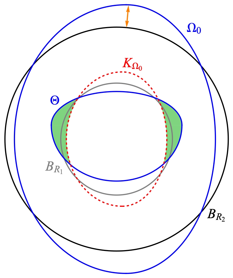
Figure 1. $\mathcal{A}_{\mathcal{H}}(\Omega_{0})$ is drawn in orange; the green set is the integration domain in the definition of $\tilde{\mathcal{A}}(\Theta;\Omega_{0})$.

We point out that the hybrid asymmetry just introduced is zero if and only if $\Omega=A_{R_{1},R_{2}}$, and so, (9) actually quantifies a deviation of an admissible set from the optimal set. The term $g(\mathcal{A}_{\mathcal{H}}(\Omega_{0}))$ quantifies the deviation with respect to the Hausdorff distance of the domain $\Omega_{0}$ from the optimal exterior shape $B_{R_{2}}$; $\tilde{\mathcal{A}}(\Theta;\Omega_{0})$ is necessary to estimate the total deviation of $\Omega$ from $A_{R_{1},R_{2}}$. Indeed, if $\Theta$ has a low Hausdorff distance from $K_{\Omega_{0}}$, then the larger term in the hybrid asymmetry is $g(\mathcal{A}(\Omega_{0}))$; on the other hand, if $\Omega_{0}$ is the ball $B_{R_{2}}$, any admissible hole $\Theta\neq B_{R_{1}}$ satisfies $\tilde{\mathcal{A}}(\Theta;B_{R_{2}})>0$ and thus in that case the largest term is $\tilde{\mathcal{A}}(\Theta;B_{R_{2}})$ (see Remark 2.10).

Moreover, $\alpha(\Omega)$ is a proper asymmetry because it holds (see Proposition 2.11) that

$$\lim_{j\to+\infty}d_{\mathcal{H}}(\Omega_{j},A_{R_{1},R_{2}})=0\iff\lim_{j\to+\infty}\alpha(\Omega_{j})=0.$$

The key idea that inspired our definition of asymmetry is the following: provided that $\Omega_{0}$ is the outer box, the most natural hole to compare $\Theta$ with is neither a ball with the same measure of $\Theta$ nor $B_{R_{1}}$, but the inner parallel $K_{\Omega_{0}}$ having the same measure as $\Theta$. This behaviour seems to depend on the fact that $K_{\Omega_{0}}$ makes the set $\Omega_{0}\setminus K_{\Omega_{0}}$ a "shell" with outer "box" $\Omega_{0}$ and fixed distance of the inner boundary $\partial K_{\Omega_{0}}$ from the outer boundary $\partial\Omega_{0}$. Moreover, the test function built via web function is constant on both $\partial K_{\Omega_{0}}$ and $\partial\Omega_{0}$. Nevertheless, the set $K_{\Omega_{0}}$ coincides with $B_{R_{1}}$ if and only if $\Omega_{0}=B_{R_{2}}$.

The main result of the paper is that inequality (4) is stable in the class $\mathcal{T}_{R_{1},R_{2}}$.

Main Theorem.

Let $0<R_{1}<R_{2}<+\infty$. There exist two positive constants $C(n,R_{1},R_{2},\beta)$ and $\delta_{0}(n,R_{1},R_{2},\beta)$ such that, for every $\Omega\in\mathcal{T}_{R_{1},R_{2}}$, if $\lambda_{1}(\beta,A)-\lambda_{1}(\beta,\Omega)\leq\delta_{0}$, then

(11) $$\lambda_{1}(\beta,A)-\lambda_{1}(\beta,\Omega)\geq C(n,R_{1},R_{2},\beta)\alpha(\Omega),$$

where $A=A_{R_{1},R_{2}}$ is the spherical shell in $\mathcal{T}_{R_{1},R_{2}}$ and $\alpha(\Omega)$ is the asymmetry defined in (9).

Our proof is based on two estimates. Since on $\partial\Omega_{0}$ a Robin boundary condition holds, we can use a Fuglede type technique on an auxiliary Steklov type problem to obtain the first estimate relative to the perturbation of the outer boundary. For this type of approach we refer to [27, 29] for the stability of the isoperimetric inequality and to [24, 30, 21] for the quantitative estimates of some spectral functionals. Then, once the outer boundary is fixed, we can estimate the deviation of $\Theta$ from $K_{\Omega_{0}}$ using the weak asymmetry $\tilde{\mathcal{A}}(\Theta;\Omega_{0})$, defined in (10) and inspired by [11, 2].

The structure of the paper is the following. In Section 2, we give some historical insights, we fix the notation, we recall some known results on the Robin-Neumann eigenvalue problem and recall some useful results on the nearly spherical sets. In Section 3 we study an auxiliary problem of Steklov type; in Section 4, we provide some quantitative estimates for $\lambda_{1}(\beta,\Omega)$ and we prove of the main result of the paper. Finally, in Section 5, a list of open problems is presented.

2. Background and Preliminary results

We start this Section by describing the historical background on problems with different boundary conditions on the outer and inner boundary. Then, we fix the notation, we recall some results on the Robin-Neumann eigenvalue problem and some properties of nearly spherical sets.

2.1. A glimpse of history

The study of spectral problems for the Robin-Laplace operator with negative parameter $\beta$ on holed domains arises from the fact that the optimal shape for the first eigenvalue, among domains with fixed volume, is expected to be the spherical shell for ${\left|\beta\right|}$ large enough. More precisely, in 1977, Bareket [7] conjectured that, among all smooth bounded domains of given volume, the first eigenvalue is maximized when $\Omega$ is a ball and, in [24], the conjecture has been proved for domains close to a ball in the $L^{\infty}$ topology. Subsequently, in [25, 38], it has been proved that the conjecture is true for small values of $\left|\beta\right|$; on the other hand, for $\left|\beta\right|$ great enough, the first Robin eigenvalue on the spherical shell is greater than the eigenvalue on the disk, among domains of fixed volume.

More recently, many authors have investigated the Laplace eigenvalue problem with different boundary conditions on the outer and inner boundary: for instance positive Robin-Neumann [42, 43], Neumann-positive Robin [23, 36], Dirichlet-Neumann [4, 5], Dirichlet-Dirichlet [9, 18], Steklov-Dirichlet [26, 31, 32, 37, 41, 46], Steklov-Robin [33].

In particular, in this paper we study a stability result for this kind of problems.

To the best of our knowledge, the quantitative improvement of spectral inequalities firstly appeared in [35, 40]; quantitative improvements of the Pólya-Szegö principle have been proven in [19]. It is worth noticing that, when $\Theta=\emptyset$, the quantitative inequalities for the Laplace eigenvalue have been studied when Dirichlet ([8, 29] and [13]), Neumann [14], positive Robin [17], negative Robin [2, 21] or Steklov [12, 30] boundary condition holds.

On the other hand, the quantitative versions of the spectral inequalities on holed domain are still in the early stages of development. We mention [41], where a result in this direction is proved for the first Steklov-Dirichlet Laplacian eigenvalue among the class of holed domains where the inner hole $\Theta$ is a given ball well cointained in $\Omega_{0}$. The inner ball can be only translated and so the only perturbation of the boundary acts on $\partial\Omega_{0}$.

Nevertheless, it seems that no results are available if a perturbation of both inner and outer boundary is kept into account.

2.2. Notations

Throughout this paper, we denote by $|\cdot|$, $P(\cdot)$ and $\mathcal{H}^{k}(\cdot)$, the $n-$dimensional Lebesgue measure, the perimeter and the $k-$dimensional Hausdorff measure in $\mathbb{R}^{n}$, respectively. The unit open ball in $\mathbb{R}^{n}$ will be denoted by $B_{1}$ and $\omega_{n}:=|B_{1}|$ and the unit sphere in $\mathbb{R}^{n}$ by $\mathbb{S}^{n-1}$. More generally, we denote with $B_{r}(x_{0})$ the set $x_{0}+rB_{1}$, that is the ball centered at $x_{0}$ with measure $\omega_{n}r^{n}$, and, for any $0<R_{1}<R_{2}<+\infty$, we denote by $A_{R_{1},R_{2}}$ the spherical shell $B_{R_{2}}\setminus\overline{B_{R_{1}}}$.

Throughout this paper, $\Omega=\Omega_{0}\setminus\overline{\Theta}$ is a subset of $\mathbb{R}^{n}$, $n\geq 2$, such that $\Omega_{0}$ is an open, bounded and convex set and $\Theta$ is a convex set such that $\overline{\Theta}\subset\Omega_{0}$.

The distance of a point from the boundary $\partial\Omega_{0}$ is the function

$$d(x)=\inf_{y\in\partial\Omega_{0}}|x-y|,\quad x\in\overline{\Omega_{0}},$$

moreover, the inradius of $\Omega_{0}$ is the radius of the largest ball contained in $\Omega_{0}$, i.e.

$$\rho({\Omega_{0}})=\max\{d(x),\;x\in\overline{\Omega_{0}}\}.$$

We denote by $J_{\nu}(r)$, $Y_{\nu}(r)$, $I_{\nu}(r)$ and $K_{\nu}(r)$ the Bessel function of first and second kind, the modified Bessel functions of the first and second kind of order $\nu$, respectively. We recall the following recurrence and derivation formulas, see [1, 47]:

(12) $$I_{\nu-1}(r)=\dfrac{2\nu}{r}I_{\nu}(r)+I_{\nu+1}(r),$$

(13) $$K_{\nu-1}(r)=-\dfrac{2\nu}{r}K_{\nu}(r)+K_{\nu+1}(r),$$

(14) $$\left(z^{-\nu}J_{\nu}(r)\right)^{\prime}=-z^{-\nu}J_{\nu+1}(r),$$

(15) $$\left(z^{-\nu}Y_{\nu}(r)\right)^{\prime}=-z^{-\nu}Y_{\nu+1}(r),$$

(16) $$\left(z^{-\nu}I_{\nu}(r)\right)^{\prime}=z^{-\nu}I_{\nu+1}(r),$$

(17) $$\left(z^{-\nu}K_{\nu}(r)\right)^{\prime}=-z^{-\nu}K_{\nu+1}(r),$$

(18) $$I_{\nu}^{\prime}(r)=\dfrac{1}{2}\left(I_{\nu-1}(r)+I_{\nu+1}(r)\right),$$

(19) $$K_{\nu}^{\prime}(r)=-\frac{1}{2}\left(K_{\nu-1}(r)+K_{\nu+1}(r)\right).$$

2.3. The Robin-Neumann eigenvalue problem

We collect now the definitions and the basic properties of the first Robin-Neumann eigenvalue; for the proofs refer to [42].

We start by recalling the weak formulation of problem (3).

Definition 2.1.

A real number $\lambda$ is an eigenvalue of (3) if and only if there exists a function $w\in H^{1}(\Omega)$, not identically zero, such that

$$\int_{\Omega}\nabla\psi\nabla\varphi\;dx+\beta\int_{\partial\Omega_{0}}\psi\varphi\;d\mathcal{H}^{n-1}=\lambda\int_{\Omega}\psi\varphi\;dx$$

for every $\varphi\in H^{1}(\Omega)$. The function $\psi$ is called the eigenfunction associated to $\lambda$.

In the following definition, we list the main properties of (1).

Proposition 2.2.

Let $\beta<0$.

• There exists a minimizer $w\in H^{1}(\Omega)$ of (1), which is a weak solution to (3).

• $\lambda_{1}(\beta,\Omega)$ is simple, i.e. all the associated eigenfunctions are scalar multiple of each other and can be taken to be positive. Moreover, $\lambda_{1}(\beta,\Omega)$ is negative.

• The map $\beta\mapsto\lambda_{1}(\beta,\Omega)$ is Lipschitz continuous, non-decreasing, concave and surjective onto $(-\infty,0)$.

• Let $R_{1},R_{2}$ be two nonnegative real numbers such that $R_{2}>R_{1}$, and let $z$ be the minimizer of problem (1) on the spherical shell $A_{R_{1},R_{2}}$. Then, $z$ is strictly positive and radially symmetric, in the sense that $z(x)=:\Psi(|x|)$, with $\Psi^{\prime}(r)>0$.

We recall now explicitly Theorem $3.1$ in [42], where it is proved that the spherical shell is the optimal shape for $\lambda_{1}(\beta,\Omega)$ when both the volume and the outer perimeter are fixed. This result holds for all $\beta\in\mathbb{R}\setminus\{0\}$, but for our purposes we state it only in the case of negative parameter.

Theorem 2.3 (Theorem $3.1$ in [42]).

Let $\beta<0$ and $A=A_{R_{1},R_{2}}$ be the spherical shell such that $|A|=|\Omega|$ and $P(B_{R_{2}})=P(\Omega_{0})$. Then,

$$\lambda_{1}(\beta,\Omega)\leq\lambda_{1}(\beta,A).$$

The test functions used in the proof of Theorem 2.3 fall in the class of the so-called web-functions (for more details refer to [34, 39, 44]), which depend only on the distance from the boundary. In particular, the authors in [42] use the following test function

$$w_{\Omega_{0}}(x):=\begin{cases}G(d(x))\quad&\text{if}\ d(x)<R_{2}-R_{1}\\ z_{m}&\text{if}\ d(x)\geq R_{2}-R_{1}\end{cases}\quad x\in\Omega_{0},$$

where $z$ is the eigenfunction of (1) on $A_{R_{1},R_{2}}$ and $G$ is defined as

$$G^{-1}(t)=\int_{t}^{z_{M}}\dfrac{1}{\ell(\tau)}\;d\tau,$$

and $\ell(t)=|\nabla z|_{z=t}$, determined for $z_{m}<t\leq z_{M}$ with $z_{m}:=\min_{A}z$ and $z_{M}:=\max_{A}z$. Moreover, $w_{\Omega_{0}}$ satisfies the following properties: $w_{\Omega_{0}}\in H^{1}(\Omega_{0})$ and

$$|\nabla w_{\Omega_{0}}|_{u=t}=|\nabla z|_{v=t},$$

$$(w_{\Omega_{0}})_{m}:=\min_{\Omega_{0}}z_{\Omega_{0}}\geq z_{m},$$

$$(w_{\Omega_{0}})_{M}:=\max_{\Omega_{0}}z_{\Omega_{0}}=z_{M}=G(0).$$

Moreover, we recall the expression of the eigenfunction $z$ associated to $\lambda=\lambda_{1}(\beta,A_{R_{1},R_{2}})$:

$$z(x)=|x|^{1-\frac{n}{2}}\left(Y_{\frac{n}{2}}(\sqrt{\lambda}R_{1})J_{\frac{n}{2}-1}(\sqrt{\lambda}|x|)-J_{\frac{n}{2}}(\sqrt{\lambda}R_{1})Y_{\frac{n}{2}-1}(\sqrt{\lambda}|x|)\right).$$

So, by the radiality of $z$, we have $z(x)=\Psi(|x|)$ and

$$\Psi(r)=r^{1-\frac{n}{2}}\delta(r),\quad\Psi^{\prime}(r)=r^{1-\frac{n}{2}}\gamma(r),$$

once having set

$$\begin{split}&\delta(r)=Y_{\frac{n}{2}}(\sqrt{\lambda}R_{1})J_{\frac{n}{2}-1}(\sqrt{\lambda}r)-J_{\frac{n}{2}}(\sqrt{\lambda}R_{1})Y_{\frac{n}{2}-1}(\sqrt{\lambda}r),\\ &\gamma(r)=-Y_{\frac{n}{2}}(\sqrt{\lambda}R_{1})J_{\frac{n}{2}}(\sqrt{\lambda}r)-J_{\frac{n}{2}}(\sqrt{\lambda}R_{1})Y_{\frac{n}{2}}(\sqrt{\lambda}r),\end{split}$$

and using (14)-(15).

Therefore, substituting $z$ in (1), we obtain

(20) $$\lambda_{1}(\beta,A_{R_{1},R_{2}})=\frac{\displaystyle\int_{R_{1}}^{R_{2}}r\gamma^{2}(r)dr+\beta R_{2}\delta^{2}(R_{2})}{\displaystyle\int_{R_{1}}^{R_{2}}r\delta^{2}(r)dr}.$$

Finally, we stress that it is possible to write the explicit expression of (20) by using the following relations for Bessel functions (see [47, eq. (10)-(11) pag. 134]):

$$\begin{split}&\int rF_{\nu}(\sqrt{\lambda}r)G_{\nu}(\sqrt{\lambda}r)dr=\frac{1}{4}r^{2}\left(2F_{\nu}(\sqrt{\lambda}r)G_{\nu}(\sqrt{\lambda}r)-F_{\nu-1}(\sqrt{\lambda}r)G_{\nu+1}(\sqrt{\lambda}r)-F_{\nu+1}(\sqrt{\lambda}r)G_{\nu-1}(\sqrt{\lambda}r)\right),\\ &\int rF^{2}_{\nu}(\sqrt{\lambda}r)dr=\frac{1}{2}r^{2}\left(F^{2}_{\nu}(\sqrt{\lambda}r)-F_{\nu-1}(\sqrt{\lambda}r)F_{\nu+1}(\sqrt{\lambda}r)\right),\end{split}$$

where $F_{\nu}$ and $G_{\nu}$ are Bessel functions of any kind of order $\nu$.

2.4. Nearly spherical sets

In this Section, we give some definitions and useful properties related to nearly spherical sets (see [27, 28]).

Definition 2.4.

Let $\Omega_{0}\subset\mathbb{R}^{n}$ be an open bounded set with $0\in\Omega_{0}$. The set $\Omega_{0}$ is said a $R-$nearly spherical set parametrized by $u$ if there exists a constant $R>0$ and $u\in W^{1,\infty}(\mathbb{S}^{n-1})$, with $||u||_{W^{1,\infty}}\leq R/2$, such that

$$\partial\Omega_{0}=\left\{y\in\mathbb{R}^{n}\colon y=\xi(R+u(\xi)),\ \xi\in\mathbb{S}^{n-1}\right\}.$$

Let us observe that the volume of a $R-$nearly spherical set is given by

$$|\Omega_{0}|=\dfrac{1}{n}\int_{\mathbb{S}^{n-1}}\left(R+u(\xi)\right)^{n}\;d\mathcal{H}^{n-1},$$

and the perimeter by

$$P(\Omega_{0})=\int_{\mathbb{S}^{n-1}}\left(R+u(\xi)\right)^{n-1}\sqrt{1+\dfrac{|\nabla_{\tau}u(\xi)|^{2}}{(R+u(\xi))^{2}}}d\mathcal{H}^{n-1},$$

where $\nabla_{\tau}u$ denotes the tangential gradient of $u$ and the tangential Jacobian of the map
$\phi:\xi\in\mathbb{S}^{n-1}\to y=R\xi(1+u(\xi))$ is

$$J_{\phi}(\xi)=(R+u(\xi))^{n-2}\sqrt{(R+u(\xi))^{2}+|\nabla_{\tau}u(\xi)|^{2}}.$$

Moreover, the unit outer normal to $\partial\Omega_{0}$ at $y=\xi(R+u(\xi))$ is given by

$$\nu(\xi)=\dfrac{\xi(R+u(\xi))-\nabla_{\tau}u(\xi)}{\sqrt{(R+u(\xi))^{2}+|\nabla_{\tau}u(\xi)|^{2}}}.$$

In the following, we deal with sets that are, in a suitable sense, close to a spherical shell and here we set the needed notation.

Definition 2.5.

Let $\Omega=\Omega_{0}\setminus\Theta$, where $\Omega_{0}$ and $\Theta$ are two convex sets such that $\Theta\subset\subset\Omega_{0}$ and $0\in\Theta$. We say that $\Omega$ is a $(R_{1},R_{2})-$nearly annular set if there exists $0<R_{1}<R_{2}<+\infty$ and $u,v\in W^{1,\infty}(\mathbb{S}^{n-1})$, with $||u||_{W^{1,\infty}}<R_{2}/2$, $||v||_{W^{1,\infty}}\leq R_{1}/2$, such that

$$\partial\Omega_{0}=\left\{y\in\mathbb{R}^{n}\colon y=\xi(R_{2}+u(\xi)),\,\xi\in\mathbb{S}^{n-1}\right\}$$

and

$$\partial\Theta=\left\{y\in\mathbb{R}^{n}\colon y=\xi(R_{1}+v(\xi)),\,\xi\in\mathbb{S}^{n-1}\right\}.$$

This definition and the outer perimeter and volume constraints yield to the following Lemma, based on the Taylor expansions.

Lemma 2.6.

There exists $C=C(n)>0$ such that, for any parametrization couple $u,v\in W^{1,\infty}(\mathbb{S}^{n-1})$ of a $(R_{1},R_{2})-$nearly annular set and for every $0<\varepsilon<R_{1}/2$ such that $||u||_{W^{1,\infty}},$ $||v||_{W^{1,\infty}}\leq\varepsilon$, the following estimates hold:

(21) $$\left|\left(R_{2}+u\right)^{n-1}-\left(R_{2}^{n-1}+(n-1)R_{2}^{n-2}u+(n-1)(n-2)R_{2}^{n-3}\frac{u^{2}}{2}\right)\right|\leq C\varepsilon R_{2}^{n-3}u^{2};$$

(22) $$\left|\left(R_{1}+v\right)^{n-1}-\left(R_{1}^{n-1}+(n-1)R_{1}^{n-2}v+(n-1)(n-2)R_{1}^{n-3}\frac{v^{2}}{2}\right)\right|\leq C\varepsilon R_{1}^{n-3}v^{2};$$

(23) $$1+\frac{|\nabla_{\tau}u|^{2}}{2R_{2}^{2}}-\sqrt{1+\dfrac{|\nabla_{\tau}u|^{2}}{(R_{2}+u)^{2}}}\leq C\varepsilon\left(u^{2}+|\nabla_{\tau}u|^{2}\right).$$

Moreover,

(24) $$\left|R_{2}^{n-2}\int_{\mathbb{S}^{n-1}}u\;d\mathcal{H}^{n-1}+\dfrac{R^{n-3}_{2}}{2(n-1)}\int_{\mathbb{S}^{n-1}}|\nabla_{\tau}u|^{2}\;d\mathcal{H}^{n-1}+\dfrac{(n-2)}{2}R_{2}^{n-3}\int_{\mathbb{S}^{n-1}}u^{2}\;d\mathcal{H}^{n-1}\right|\leq C\varepsilon,$$

and

(25) $$\begin{split}\left|R_{1}^{n-1}\int_{\mathbb{S}^{n-1}}v\;d\mathcal{H}^{n-1}+\right.&\dfrac{(n-1)}{2}R_{1}^{n-1}\int_{\mathbb{S}^{n-1}}v^{2}\;d\mathcal{H}^{n-1}\\ &\left.-R_{2}^{n-1}\int_{\mathbb{S}^{n-1}}u\;d\mathcal{H}^{n-1}-\dfrac{(n-1)}{2}R_{2}^{n-1}\int_{\mathbb{S}^{n-1}}u^{2}\;d\mathcal{H}^{n-1}\right|\leq C\varepsilon.\end{split}$$

Proof.

The proofs of (21)-(25) can be immediately adapted from [27]. Inequalities (21) and (22) easily follow, respectively, from

(26) $$(R_{2}+u)^{n-1}=\sum_{k=0}^{n-1}\binom{n-1}{k}u^{k}R_{2}^{n-1-k}\quad\text{and}\quad(R_{1}+v)^{n-1}=\sum_{k=0}^{n-1}\binom{n-1}{k}v^{k}R_{1}^{n-1-k}.$$

Inequality (23) is a consequence of inequality $\sqrt{1+x}\geq 1+\frac{x}{2}-\frac{x^{2}}{4}$. Furthermore, using the outer perimeter constraint

$$\frac{1}{n}\int_{\mathbb{S}^{n-1}}(R_{2}+u)^{n-1}\sqrt{1+\dfrac{|\nabla u|^{2}}{(R_{2}+u)^{2}}}d\mathcal{H}^{n-1}=\omega_{n}R_{2}^{n-1},$$

the first equality in (26) and (23), we obtain (24). Finally, inequality (25) follows by using the volume constraint

$$\frac{1}{n}\int_{\mathbb{S}^{n-1}}(R_{2}+u)^{n-1}-(R_{1}+v)^{n-1}d\mathcal{H}^{n-1}=\omega_{n}(R_{2}^{n-1}-R_{1}^{n-1})$$

and the second equality in (26). ∎

The Poincaré inequality in this setting holds with constant $(n-1)$, but, since we are working with functions parametrizing nearly spherical sets, this constant can been improved to $2n$. For the proof we refer to [27] and [24, Lem. 2.4].

Lemma 2.7.

There exists a constant $C>0$ such that, for any parametrization $u\in W^{1,\infty}(\mathbb{S}^{n-1})$ of a $R-$nearly spherical set and for every $0<\varepsilon<R/2$ with $||u||_{W^{1,\infty}}\leq\varepsilon$, it holds

(27) $$||\nabla_{\tau}u||_{L^{2}}^{2}\geq 2n||u||_{L^{2}}^{2}-\varepsilon C.$$

Finally, these last two Lemmata provide key estimates for the norms of functions parametrizing the boundary of a nearly spherical set, see [27, 28].

Lemma 2.8.

Let $u\in W^{1,\infty}(\mathbb{S}^{n-1})$ such that $\displaystyle\int_{\mathbb{S}^{n-1}}u\;d\mathcal{H}^{n-1}=0$, then

$$||u||_{L^{\infty}}^{n-1}\leq\begin{cases}\pi\|\nabla_{\tau}u\|_{L^{2}}&n=2\\ 4||\nabla_{\tau}u||^{2}_{L^{2}}\log\frac{8e||\nabla_{\tau}u||_{L^{\infty}}^{n-1}}{||\nabla_{\tau}u||_{L^{2}}^{2}}&n=3\\[5.69046pt] C(n)||\nabla_{\tau}u||_{L^{2}}^{2}||\nabla_{\tau}u||_{L^{\infty}}^{n-3}\,\,&n\geq 4.\end{cases}$$

Lemma 2.9.

Let $u\in W^{1,\infty}(\mathbb{S}^{n-1})$ be a parametrization of a $R-$nearly spherical set such that $||u||_{W^{1,\infty}}<\varepsilon$ for some $\varepsilon<R/2$, then

$$||\nabla_{\tau}u||_{\infty}\leq 3||u||_{\infty}^{\frac{1}{2}}.$$

2.5. Some properties of the hybrid asymmetry

In this Section we focus on some properties of the hybrid asymmetry $\alpha(\Omega)$, see Definition 1.1. First of all, we show that $\alpha(\Omega)=0$ if and only if $\Omega=A_{R_{1},R_{2}}$.

Remark 2.10.

We point out that $\tilde{\mathcal{A}}(\Theta;\Omega_{0})\geq 0$, but it could be zero even if $\Omega_{0}\neq B_{R_{2}}$ and $\Theta\neq K_{\Omega_{0}}$. Indeed, if

$$d_{\mathcal{H}}(\Theta,K_{\Omega_{0}})<t_{\Omega_{0}}-(R_{2}-R_{1}),$$

then $\tilde{\mathcal{A}}(\Theta;\Omega_{0})=0$. Nevertheless, in that case, $\Omega_{0}\neq B_{R_{2}}$, thus the global asymmetry satisfies

$$\alpha(\Omega)=\max\left\{g(\mathcal{A}_{\mathcal{H}}(\Omega_{0})),\tilde{\mathcal{A}}(\Theta;\Omega_{0})\right\}=g(\mathcal{A}_{\mathcal{H}}(\Omega_{0}))>0.$$

In other words, if $\Theta$ has a low Hausdorff distance from $K_{\Omega_{0}}$, then the larger term in the computation of $\alpha(\Omega)$ is $g(\mathcal{A}(\Omega_{0}))$. In particular we point out that, provided that $\Theta\neq K_{\Omega_{0}}$, $\tilde{\mathcal{A}}(\Theta;\Omega_{0})$ could be zero if and only if $\Omega_{0}\neq B_{R_{2}}$.

On the other hand, we stress the fact that $t_{\Omega_{0}}=R_{2}-R_{1}$ if and only if $\Omega_{0}=B_{R_{2}}$. So, in this case, $K_{\Omega_{0}}=B_{R_{1}}$ and any admissible hole $\Theta\neq B_{R_{1}}$ satisfies $\tilde{\mathcal{A}}(\Theta;B_{R_{2}})>0$, since $w_{\Omega_{0}}=z\gneq z_{m}$ on $\Theta\setminus B_{R_{1}}$. Consequently, we have

$$\alpha(\Omega)=\max\left\{g(\mathcal{A}_{\mathcal{H}}(B_{R_{2}})),\tilde{\mathcal{A}}(\Theta;B_{R_{2}})\right\}=\tilde{\mathcal{A}}(\Theta;B_{R_{2}})>0.$$

So, it actually holds $\alpha(\Omega)=0$ if and only if $\Omega=A_{R_{1},R_{2}}$.

Now, we justify the fact that $\alpha(\Omega)$ is actually an asymmetry in the sense that the set $\Omega$ tends to the spherical shell $A_{R_{1},R_{2}}$ in the Hausdorff sense if and only if the hydrid asymmetry $\alpha(\Omega)$ tends to zero.

Proposition 2.11.

Let $0<R_{1}<R_{2}<+\infty$ and $\Omega_{j}\subset\mathbb{R}^{n}$ in the class $\mathcal{T}_{R_{1},R_{2}}$. Then

$$\lim_{j\to+\infty}d_{\mathcal{H}}(\Omega_{j},A_{R_{1},R_{2}})=0\iff\lim_{j\to+\infty}\alpha(\Omega_{j})=0.$$

Proof.

The necessary implication directly follows from Definition 1.1. Therefore, it only remains to prove the converse condition.

Let $\{\Omega_{j}\}_{j\in\mathbb{N}}$ be a sequence such that $\alpha(\Omega_{j})\to 0$. Since $\Omega_{j}\in\mathcal{T}_{R_{1},R_{2}}$ for any $j\in\mathbb{N}$, then $\Omega_{j}=(\Omega_{0})_{j}\setminus\Theta_{j}$. Consequently, from Definition 1.1, it is clear that $d_{\mathcal{H}}({\Omega_{0}}_{j},B_{R_{2}})\to 0$.

By contradiction, let us assume that $d_{\mathcal{H}}(\Theta j,B_{R_{1}})>c$. We have two possibilities: the difference between $\Theta$ and $B_{R_{1}}$ is more concentrated either inside or outside $B_{R_{1}}$. Specifically

1. there exists $x_{j}\in\Theta_{j}\cap B_{R_{1}}$ such that $d(x_{j},B_{R_{1}})>c$ and $d_{\mathcal{H}}(\partial\Theta_{j}\setminus B_{R_{1}},B_{R_{1}})\to 0$;

2. there exists $x_{j}\in\Theta_{j}\setminus B_{R_{1}}$ such that $d(x_{j},B_{R_{1}})>c$.

In the case (i), the volume constraint gives the contradiction. Indeed, there exists $\bar{j}$ such that $|\Theta_{j}|<|B_{R_{1}}|-c$, for any $j>\bar{j}$. From the volume constraint, we have an absurd, since it would be $|\Omega_{j}|\geq|A_{R_{1},R_{2}}|+c$.

Now, we consider the case (ii), where a key role is played by the set $({\Omega_{0}}_{j})_{R_{2}-R_{1}}$, in which, by the definition (8), the test function $w_{\Omega_{0}}$ is constant.

We point out that, in view of the behavior of the outer asymmetry, we have $d_{\mathcal{H}}(B_{R_{1}},({\Omega_{0}}_{j})_{R_{2}-R_{1}})\to 0$; in particular, there exists $c>0$ such that $d_{\mathcal{H}}(({\Omega_{0}}_{j})_{R_{2}-R_{1}},B_{R_{1}})<c/2$. This inequality, together with the assumption (ii), implies that there exists two positive constants $c$ and $c^{\prime}$ such that $d_{\mathcal{H}}(({\Omega_{0}}_{j})_{R_{2}-R_{1}},\Theta_{j})>c/2$ and, in view of the inradius constraint in the class $\mathcal{T}_{R_{1},R_{2}}$, it holds $|\Theta_{j}\setminus({\Omega_{0}}_{j})_{R_{2}-R_{1}}|>c^{\prime}/2$.

Since, by construction and by the volume constraint, we have that $K_{(\Omega_{0})_{j}}\subseteq({\Omega_{0}}_{j})_{R_{2}-R_{1}}$, then $d(x)<R_{2}-R_{1}-c/2$ and hence $w_{(\Omega_{0})_{j}}(x)>G(R_{2}-R_{1}-c/2)$ on $\Theta_{j}\setminus K_{(\Omega_{0})_{j}}$. Consequently, there exists $c^{\prime\prime}>0$ such that

$$\tilde{\mathcal{A}}(\Theta_{j},{\Omega_{0}}_{j})=\int_{\Theta_{j}\setminus K_{(\Omega_{0})_{j}}}w_{(\Omega_{0})_{j}}^{2}(x)-z_{m}^{2}\ dx>c^{\prime\prime}>0,$$

that is absurd.

Therefore, in both cases we contradict the assumption $d_{\mathcal{H}}(\Theta j,B_{R_{1}})>c$. Hence we conclude. ∎

Let us observe that, if we denote by $\chi_{E}$ the characteristic function of a set $E$, then the weak weighted Fraenkel asymmetry (10) can be also written as

$$\tilde{\mathcal{A}}(\Theta,{\Omega_{0}})=\int_{\mathbb{R}^{n}}\chi_{\Theta\setminus K_{\Omega_{0}}}(w_{\Omega_{0}}^{2}(x)-z_{m}^{2})dx.$$

Finally, it is worth noticing that

$$\tilde{\mathcal{A}}(\Theta,{\Omega_{0}})\geq||w_{\Omega_{0}}-z_{m}||^{2}_{L^{2}(\Theta\setminus K_{\Omega_{0}})}.$$

3. A quantitative result for a Steklov-type problem

The quantitative results for the Robin eigenvalue problem with negative boundary parameter are often solved through Steklov type problems (see [6, 21, 24]). This strategy is suggested by a similar behavior of the functionals in terms of monotonicity and of eigenfunctions. Indeed, as a first trivial link between the two functionals, one can observe that the Rayleigh quotients of both the Robin and the Steklov first eigenvalues are monotonically decreasing with respect to the boundary integral.

The strategy of the proof is inspired by [21, 24], where the authors relate the Raylegh quotient of a suitable Steklov-type eigenvalue problem with a ratio involving only the boundary integral terms. Subsequently, the suitable representations of the outer and inner boundary are useful to estimate the difference between the eigenvalues on the radial and on the quasi-radial shape.

3.1. A Steklov-type problem

The auxiliary problem we deal with is the following:

(28) $$\sigma_{1}(\Omega)=\min_{\begin{subarray}{c}\psi\in H^{1}(\Omega)\\ \psi\not\equiv 0\end{subarray}}\dfrac{\displaystyle\int_{\Omega}|\nabla\psi|^{2}+\int_{\Omega}\psi^{2}\;dx}{\displaystyle\int_{\partial\Omega_{0}}\psi^{2}\;d\mathcal{H}^{n-1}}.$$

If $w\in H^{1}(\Omega)$ is a minimizer of (29), then it satisfies:

(29) $$\begin{cases}-\Delta w+w=0&\mbox{in}\ \Omega\vspace{0.2cm}\\ \dfrac{\partial w}{\partial\nu}=\sigma_{1}(\Omega)w&\mbox{on}\ \partial\Omega_{0}\vspace{0.2cm}\\ \dfrac{\partial w}{\partial\nu}=0&\text{on }\partial\Theta.\end{cases}$$

If $\Omega$ is the spherical shell $A_{R_{1},R_{2}}=B_{R_{2}}\setminus\overline{B}_{R_{1}}$, the unique solution (up to multiplicative constant) of problem (28) is radial and it is given by

$$z(x)=\Psi(|x|),$$

where

(30) $$\Psi(r)=r^{1-\frac{n}{2}}K_{\frac{n}{2}}(R_{1})I_{\frac{n}{2}-1}(r)+r^{1-\frac{n}{2}}I_{\frac{n}{2}}(R_{1})K_{\frac{n}{2}-1}(r)\quad\forall r\in[R_{1},R_{2}].$$

The starting point of our analysis is the following upper bound for $\sigma_{1}(\Omega)$, only involving outer boundary integral terms.

Lemma 3.1.

It holds that

(31) $$\sigma_{1}(\Omega)\leq\dfrac{\displaystyle\int_{\partial\Omega_{0}}z\dfrac{\partial z}{\partial\nu}\;d\mathcal{H}^{n-1}}{\displaystyle\int_{\partial\Omega_{0}}z^{2}\;d\mathcal{H}^{n-1}}=:\dfrac{N(\Omega)}{D(\Omega)},$$

where $z(x)=\Psi(|x|)$ is defined in (30). Moreover, equality in (31) holds iff $\Omega=A_{R_{1},R_{2}}$, that is the spherical shell with the same volume of $\Omega$ and such that $P(\Omega_{0})=P(B_{R_{2}})$.

Proof.

Let $w\in H^{1}(\Omega)$ be a solution of (28). For every $\varphi\in H^{1}(\Omega)$, we have that

$$0=\displaystyle\int_{\Omega}\varphi w\;dx-\displaystyle\int_{\Omega}\varphi\Delta w\;dx=\displaystyle\int_{\Omega}\varphi w\;dx+\displaystyle\int_{\Omega}\nabla\varphi\nabla w\;dx-\displaystyle\int_{\partial\Omega_{0}}\varphi\dfrac{\partial w}{\partial\nu}\;d\mathcal{H}^{n-1}=$$

$$=\displaystyle\int_{\Omega}\varphi w\;dx+\displaystyle\int_{\Omega}\nabla\varphi\nabla w\;dx-\sigma_{1}(\Omega)\displaystyle\int_{\partial\Omega_{0}}\varphi w\;d\mathcal{H}^{n-1}.$$

Therefore, we have

$$\sigma_{1}(\Omega)\displaystyle\int_{\partial\Omega_{0}}\varphi w\;d\mathcal{H}^{n-1}=\displaystyle\int_{\Omega}\varphi w\;dx+\displaystyle\int_{\Omega}\nabla\varphi\nabla w\;dx.$$

If we choose $\varphi=w$, the divergence theorem and the fact that $w$ is a solution of (29) lead to

$$\sigma_{1}(\Omega) =\dfrac{\displaystyle\int_{\Omega}w^{2}\;dx+\displaystyle\int_{\Omega}|\nabla w|^{2}\;dx}{\displaystyle\int_{\partial\Omega_{0}}w^{2}\;d\mathcal{H}^{n-1}}=$$

$$=\dfrac{\displaystyle\int_{\Omega}w^{2}\;dx-\displaystyle\int_{\Omega}w\Delta w\;dx+\displaystyle\int_{\partial\Omega_{0}}w\dfrac{\partial w}{\partial\nu}\;d\mathcal{H}^{n-1}}{\displaystyle\int_{\partial\Omega_{0}}w^{2}\;d\mathcal{H}^{n-1}}=\dfrac{\displaystyle\int_{\partial\Omega_{0}}w\dfrac{\partial w}{\partial\nu}\;d\mathcal{H}^{n-1}}{\displaystyle\int_{\partial\Omega_{0}}w^{2}\;d\mathcal{H}^{n-1}}.$$

In this way, we have obtained the variational characterization of $\sigma_{1}(\Omega)$:

(32) $$\sigma_{1}(\Omega)=\min_{\begin{subarray}{c}\psi\in H^{1}(\Omega)\\ \psi\not\equiv 0\end{subarray}}\dfrac{\displaystyle\int_{\partial\Omega_{0}}\psi\dfrac{\partial\psi}{\partial\nu}\;d\mathcal{H}^{n-1}}{\displaystyle\int_{\partial\Omega_{0}}\psi^{2}\;d\mathcal{H}^{n-1}}.$$

Finally, let $z$ be the solution of (28) when $\Omega$ is the spherical shell; the claimed result follows by testing the problem (32) with $z$. ∎

3.2. The weighted quotient

Now, our aim is to write the ratio in the right-hand side of (31) in the case when $\Omega_{0}$ is a $R_{2}$-nearly spherical set. It is worth noticing that, since in (31) an interior boundary term is not appearing, the same variational characterization holds when $\Omega$ is a $(R_{1},R_{2})-$nearly annular set.

Keeping in mind the radial solution (30), we define

(33) $$\eta(r)=\left[K_{\frac{n}{2}}(R_{1})I_{\frac{n}{2}-1}(r)+I_{\frac{n}{2}}(R_{1})K_{\frac{n}{2}-1}(r)\right]\quad\forall r\in[R_{1},R_{2}],$$

(34) $$\mu(r)=\left[K_{\frac{n}{2}}(R_{1})I_{\frac{n}{2}}(r)-I_{\frac{n}{2}}(R_{1})K_{\frac{n}{2}}(r)\right]\quad\forall r\in[R_{1},R_{2}],$$

where the second relation is obtained by deriving the first one with the use of the derivative rules (16) and (17).

We observe that both the quantities $\eta(r)$ and $\mu(r)$ are strictly positive. Indeed, $\eta>0$ is trivially verified and, as far as $\mu$ is concerned, for any $\nu>-1$, we have that

$$\dfrac{I_{\nu+1}}{K_{\nu+1}}(R_{1})<\dfrac{I_{\nu+1}}{K_{\nu+1}}(r)$$

for any $r>R_{1}$, since

$$\frac{d}{dt}\left[\dfrac{I_{\nu}}{K_{\nu}}(r)\right]=\dfrac{\left(I_{\nu-1}(r)+I_{\nu+1}(r)\right)K_{\nu}(r)+I_{\nu}(r)\left(K_{\nu-1}(r)+K_{\nu+1}(r)\right)}{2K_{\nu}(x)^{2}}>0.$$

Furthermore, the monotonicity of $I_{\nu}$ and $K_{\nu}$ with respect to the index (see as a reference [22]) implies that $\eta(r)>\mu(r)$ . Let us observe that, by (16) and (17), the following derivation rules also hold:

(35) $$\left(r^{1-\frac{n}{2}}\eta(r)\right)^{\prime}=r^{1-\frac{n}{2}}\mu(r);\quad\left(r^{\frac{n}{2}}\mu(r)\right)^{\prime}=r^{\frac{n}{2}}\eta(r);$$

(36) $$\eta^{\prime}(r)=\left(\frac{n}{2}-1\right)\frac{\eta(r)}{r}+\mu(r);\qquad\mu^{\prime}(r)=-\frac{n}{2}\frac{\mu(r)}{r}+\eta(r).$$

Hence, the functions $\eta$ and $\mu$, defined in (33) and (34) respectively, lead to the definitions of the integrand functions in the quotient (31), that are

(37) $$h(r)=r^{2-n}\eta^{2}(r)\quad\forall r\in[R_{1},R_{2}],$$

(38) $$f(r)=\frac{h^{\prime}(r)}{2}=r^{2-n}\eta(r)\mu(r)\quad\forall r\in[R_{1},R_{2}].$$

Finally, using the parametrization of $R_{2}-$nearly spherical sets (see Definition (2.4)), we get:

(39) $$N(\Omega)=\displaystyle\int_{\mathbb{S}^{n-1}}f(R_{2}+u)\left(R_{2}+u\right)^{n-1}\;d\mathcal{H}^{n-1},$$

(40) $$D(\Omega)=\displaystyle\int_{\mathbb{S}^{n-1}}h(R_{2}+u)\left(R_{2}+u\right)^{n-1}\sqrt{1+\dfrac{|\nabla_{\tau}u|^{2}}{\left(R_{2}+u\right)^{2}}}\;d\mathcal{H}^{n-1}.$$

Let us notice that, in the case $\Omega=A_{R_{1},R_{2}}$, we have

$$\sigma_{1}(A_{R_{1},R_{2}})=\dfrac{f(R_{2})}{h(R_{2})}.$$

The following Lemma is a consequence of the fact that the functions $h$ and $f$ defined in (37) and (38) are analytic.

Lemma 3.2.

For any parametrization couple $u,v\in W^{1,\infty}(\mathbb{S}^{n-1})$ of a $(R_{1},R_{2})-$nearly annular set and for every $0<\varepsilon<R_{1}/2$ such that $||u||_{W^{1,\infty}},||v||_{W^{1,\infty}}\leq\varepsilon$, there exists $C=C(n,R_{1},R_{2})>0$ such that, on $\mathbb{S}^{n-1}$, we have:

(41) $$\left|h(R_{2}+u)-h(R_{2})-h^{\prime}(R_{2})u-h^{\prime\prime}(R_{2})\frac{u^{2}}{2}\right|\leq K\varepsilon u^{2},$$

(42) $$\left|h(R_{1}+v)-h(R_{1})-h^{\prime}(R_{1})v-h^{\prime\prime}(R_{1})\frac{v^{2}}{2}\right|\leq K\varepsilon v^{2},$$

(43) $$\left|f(R_{2}+u)-f(R_{2})-f^{\prime}(R_{2})u-f^{\prime\prime}(R_{2})\frac{u^{2}}{2}\right|\leq K\varepsilon u^{2}.$$

The following monotonicity result will be useful in proving the stability result for $\sigma_{1}(\Omega)$. The proof generalizes a result contained in [3].

Lemma 3.3.

For any $R_{1}>0$, we have that

$$\left(\frac{\eta(r)}{\mu(r)}\right)^{\prime}<0\quad\forall\ r\geq R_{1},$$

where $\eta$ and $\mu$ are defined in (33) and (34).

Proof.

Since $\eta(r)$ is a linear combination of the modified Bessel functions $I_{\nu}$ and $K_{\nu}$, it satisfies the following equation:

$$\eta^{\prime\prime}+\frac{1}{r}\eta^{\prime}-\frac{r^{2}+(\frac{n}{2}-1)^{2}}{r^{2}}\eta=0,$$

that is

$$r^{2}\eta^{\prime}\eta^{\prime\prime}+r\eta^{\prime 2}-\left(r^{2}+\left(\frac{n}{2}-1\right)^{2}\right)\eta\eta^{\prime}=0,$$

i.e.

$$r\eta^{\prime}(r\eta^{\prime})^{\prime}-\left(r^{2}+\left(\frac{n}{2}-1\right)^{2}\right)\eta\eta^{\prime}=0.$$

Therefore, dividing by $r\eta^{\prime}$, we obtain:

(44) $$(r\eta^{\prime})^{\prime}=\frac{r^{2}+(\frac{n}{2}-1)^{2}}{r}\eta.$$

In the same way, we also gain:

(45) $$(r\mu^{\prime})^{\prime}=\frac{r^{2}+(\frac{n}{2})^{2}}{r}\mu.$$

By using (44) and (45), we are able to write the following equality

$$\int_{0}^{r}[\eta(s\mu^{\prime})^{\prime}-\mu(s\eta^{\prime})^{\prime}]ds=(n-1)\int_{0}^{r}\frac{\eta(s)\mu(s)}{s}ds>0.$$

By applying the Green Theorem on the l.h.s, we have

$$s[\eta\mu^{\prime}-\mu\eta^{\prime}]_{0}^{r}=(n-1)\int_{0}^{r}\frac{\eta(s)\mu(s)}{s}ds>0,$$

that leads to

(46) $$\frac{\mu^{\prime}(r)}{\mu(r)}-\frac{\eta^{\prime}(r)}{\eta(r)}=\frac{n-1}{r\eta(r)\mu(r)}\int_{0}^{r}\frac{\eta(s)\mu(s)}{s}ds>0\quad\forall r>0.$$

By using the relation (46), the thesis follows by observing that

$$\left(\dfrac{\eta(r)}{\mu(r)}\right)^{\prime}=\frac{\eta^{\prime}(r)\mu(r)-\eta(r)\mu^{\prime}(r)}{\mu^{2}(r)}=\frac{\eta^{\prime}(r)\mu(r)-\eta(r)\mu^{\prime}(r)}{\mu(r)\eta(r)}\frac{\eta(r)}{\mu(r)}=\left(\frac{\eta^{\prime}(r)}{\eta(r)}-\frac{\mu^{\prime}(r)}{\mu(r)}\right)\frac{\eta(r)}{\mu(r)}<0.$$

∎

We end this section with a very technical Lemma establishing the sign of a certain quantity, that will be useful to obtain the stability result. The proof is based on the second part of [24, Prop. 2.5]. For sake of simplicity, we set:

(47) $$\begin{split}A_{0}=&R_{2}^{n-1}f(R_{2})h(R_{2}),\\ A_{1}=&R_{2}^{n-1}[f(R_{2})h^{\prime}(R_{2})-f^{\prime}(R_{2})h(R_{2})],\\ A_{2}=&R_{2}^{n-1}[f(R_{2})h^{\prime\prime}(R_{2})-f^{\prime\prime}(R_{2})h(R_{2})].\end{split}$$

Lemma 3.4.

For any $R_{2}>0$, we have that

(48) $$(n-1)R_{2}A_{1}+R_{2}^{2}A_{2}+2nA_{0}>0.$$

Proof.

If we put in evidence $R_{2}^{2}$ in (48), we obtain $R_{2}^{2}[\frac{(n-1)}{R_{2}}A_{1}+A_{2}+\frac{2n}{R_{2}^{2}}A_{0}]>0$ and, so, we have to prove that

$$\left[\frac{(n-1)}{R_{2}}A_{1}+A_{2}+\frac{2n}{R_{2}^{2}}A_{0}\right]=[r^{n-1}(f(r)h^{\prime}(r)-h(r)f^{\prime}(r)]^{\prime}+2nr^{n-3}h(r)f(r)>0$$

for $r=R_{2}$. By using the definitions of $h$ and $f$ in (37)-(38) and the derivation rules (35), the last relation becomes

$$[r^{2-n}(r\eta^{2}(r)\mu^{2}(r)-r\eta^{4}(r)+(n-1)\eta^{3}(r)\mu(r))]^{\prime}+2nr^{1-n}\eta^{3}(r)\mu(r)>0$$

and hence

$$r^{1-n}\eta(r)\mu(r)[2r^{2}\mu^{2}(r)+2(n-1)r\eta(r)\mu(r)+(n+1-2r^{2})\eta^{2}(r)]>0.$$

If we set

$$\zeta(r):=2r^{2}\mu^{2}(r)+2(n-1)r\eta(r)\mu(r)+(n+1-2r^{2})\eta^{2}(r),$$

we need to show that $\zeta(r)>0$. We observe that

$$\zeta^{\prime}(r)=\frac{1}{r}\bigl{(}\zeta(r)+4r\eta(r)\mu(r)+(n^{2}-2n-3)\eta^{2}(r)\bigr{)}.$$

If $n\geq 3$, since $n^{2}-2n-3\geq 0$ and $\eta(r),\mu(r)>0$ for any $r>0$, we deduce that $r\zeta^{\prime}(r)\geq\zeta(r)$ and hence that $\zeta(r)>0$ for any $r>0$. Otherwise, if $n=2$, we observe that the function $\xi(r)=r\zeta^{\prime}(r)$ is increasing for $r>0$ because, by using (36), we have that

$$\xi^{\prime}(r)=(r\zeta^{\prime}(r))^{\prime}=6r\mu^{2}(r)+2r\eta^{2}(r)>0\quad\forall r>0.$$

Moreover, it is immediate that $\xi^{\prime}(0)=\xi(0)=0$. This means that $\xi(r)>0$ and hence $\zeta^{\prime}(r)>0$ for any $r>0$. Finally, since $\zeta(0)=0$, this implies that $\zeta(r)>0$ for any $r>0$. ∎

3.3. The stability result

A crucial result to obtain the stability with respect to the outer boundary is the following stability issue for the functional $\Omega\mapsto\frac{N(\Omega)}{D(\Omega)}$. Up to some necessary technical modification, the proof follows the scheme in [21, 24].

Proposition 3.5.

Let $0<R_{1}<R_{2}<+\infty$. There exists $C_{1}=C_{1}(n,R_{1},R_{2})>0$ such that, for any $(R_{1},R_{2})-$nearly annular set $\Omega$ with the outer boundary parametrized by $u\in W^{1,\infty}(\mathbb{S}^{n-1})$, and for every $0<\varepsilon<R_{1}/2$ such that $||u||_{W^{1,\infty}}\leq\varepsilon$, the following stability inequality holds true:

$$\frac{N(\Omega^{\#})D(\Omega)-D(\Omega^{\#})N(\Omega)}{n\omega_{n}}\geq C_{1}(n,R_{1},R_{2})||\nabla_{\tau}u||_{L^{2}}^{2}.$$

Proof.

We start by performing a suitable “Taylor expansion” in terms of the deformations of $\partial\Omega_{0}$ compared to $\partial B_{R_{2}}$. By using the characterization of $N(\Omega)$ and $D(\Omega)$ in (39) and (40), we obtain

$$\begin{split}\frac{N(\Omega^{\#})D(\Omega)-D(\Omega^{\#})N(\Omega)}{n\omega_{n}}&=f(R_{2})\int_{\mathbb{S}^{n-1}}h(R_{2}+u)(R_{2}+u)^{n-1}\sqrt{1+\frac{|\nabla_{\tau}u|^{2}}{(R_{2}+u)^{2}}}\;d\mathcal{H}^{n-1}\\ &\quad-h(R_{2})\int_{\mathbb{S}^{n-1}}f(R_{2}+u)(R_{2}+u)^{n-1}\;d\mathcal{H}^{n-1}.\end{split}$$

Then, by using the Lemmata 2.6 and 3.2, we get

(49) $$\begin{split}\frac{N(\Omega^{\#})D(\Omega)-D(\Omega^{\#})N(\Omega)}{n\omega_{n}}&\geq\int_{\mathbb{S}^{n-1}}R_{2}^{2n-2}[f(R_{2})h^{\prime}(R_{2})-f^{\prime}(R_{2})h(R_{2})]u\;d\mathcal{H}^{n-1}\\ &\quad+\int_{\mathbb{S}^{n-1}}R_{2}^{2n-3}[2(n-1)(f(R_{2})h^{\prime}(R_{2})-f^{\prime}(R_{2})h(R_{2}))]\frac{u^{2}}{2}\;d\mathcal{H}^{n-1}\\ &\quad+\int_{\mathbb{S}^{n-1}}R_{2}^{2n-2}[f(R_{2})h^{\prime\prime}(R_{2})-f^{\prime\prime}(R_{2})h(R_{2})]\frac{u^{2}}{2}\;d\mathcal{H}^{n-1}\\ &\quad+\int_{\mathbb{S}^{n-1}}R_{2}^{2n-4}f(R_{2})h(R_{2})\frac{|\nabla_{\tau}u|^{2}}{2}\;d\mathcal{H}^{n-1}-\varepsilon C_{1}\|\nabla_{\tau}u\|^{2}_{L^{2}}.\\ \end{split}$$

Now, using the notation in (47), inequality (49) becomes

(50) $$\begin{split}\frac{N(\Omega^{\#})D(\Omega)-D(\Omega^{\#})N(\Omega)}{n\omega_{n}}&\geq R_{2}^{n-1}A_{1}\int_{\mathbb{S}^{n-1}}u\;d\mathcal{H}^{n-1}+R_{2}^{n-2}[2(n-1)A_{1}+R_{2}A_{2}]\int_{\mathbb{S}^{n-1}}\frac{u^{2}}{2}\;d\mathcal{H}^{n-1}\\ &\quad+R_{2}^{n-3}A_{0}\int_{\mathbb{S}^{n-1}}\frac{|\nabla_{\tau}u|^{2}}{2}\;d\mathcal{H}^{n-1}-\varepsilon C_{1}\|\nabla_{\tau}u\|^{2}_{L^{2}}.\end{split}$$

Moreover, by the perimeter constraint given by (24), then (50) becomes

(51) $$\begin{split}\frac{N(\Omega^{\#})D(\Omega)-D(\Omega^{\#})N(\Omega)}{n\omega_{n}}&\geq R_{2}^{n-2}\frac{nA_{1}+R_{2}A_{2}}{2}\int_{\mathbb{S}^{n-1}}u^{2}\;d\mathcal{H}^{n-1}\\ &\quad+R_{2}^{n-3}\left(\frac{A_{0}}{2}-\frac{R_{2}A_{1}}{2(n-1)}\right)\int_{\mathbb{S}^{n-1}}|\nabla_{\tau}u|^{2}\;d\mathcal{H}^{n-1}-\varepsilon C_{1}\|\nabla_{\tau}u\|^{2}_{L^{2}}.\end{split}$$

Firstly, let us note that the term in round parenthesis is positive because it is the sum of two positive terms. Indeed, $A_{0}$, defined in (47), is positive, since $h>0$ and $f>0$ (defined respectevely in (37) and (38)); meanwhile

(52) $$A_{1}=R_{2}^{n-1}[f(R_{2})h^{\prime}(R_{2})-f^{\prime}(R_{2})h(R_{2})]=f^{2}(R_{2})\left[\frac{h(r)}{f(r)}\right]^{\prime}_{r=R_{2}}=f^{2}(R_{2})\left[\frac{\eta(r)}{\mu(r)}\right]^{\prime}_{r=R_{2}}<0,$$

where the last inequality follows from Lemma 3.3.

Therefore, since it is possible to take $\varepsilon C_{1}$ arbitrarily small, where the quantity $C_{1}$ does not depend on $\varepsilon$, the proof is concluded if we verify that

(53) $$\frac{nA_{1}+R_{2}A_{2}}{2}\geq 0.$$

Otherwise, if (53) does not hold (i.e. if $\frac{nA_{1}+R_{2}A_{2}}{2}<0$), we go on with the estimate from below. More precisely, by using the Poicarè inequality (27), from (51), we get

$$\begin{split}\frac{N(\Omega^{\#})D(\Omega)-D(\Omega^{\#})N(\Omega)}{n\omega_{n}}&\geq\frac{R_{2}^{n-3}}{4n}\left(\frac{n^{2}-3n}{n-1}R_{2}A_{1}+R_{2}^{2}A_{2}+2nA_{0}\right)\int_{\mathbb{S}^{n-1}}|\nabla_{\tau}u|^{2}\;d\mathcal{H}^{n-1}\\ &\quad-\varepsilon C_{1}\|\nabla_{\tau}u\|^{2}_{L^{2}}.\end{split}$$

Finally, in order to conclude the proof, it remains to show that

$$\left(\frac{n^{2}-3n}{n-1}R_{2}A_{1}+R_{2}^{2}A_{2}+2nA_{0}\right)>0.$$

This term can be written as the sum of two positive quantities in the following way:

$$\frac{n^{2}-3n}{n-1}R_{2}A_{1}+R_{2}^{2}A_{2}+2nA_{0}=\left[(n-1)R_{2}A_{1}+R_{2}^{2}A_{2}+2nA_{0}\right]-\frac{n+1}{n-1}R_{2}A_{1}.$$

Indeed, the positive sign of the first addendum of the right hand side of the last equality is proved in Lemma 3.4 and the sign of the second one follows from (52). ∎

An immediate consequence of Proposition 3.5 is the following stability result for $\sigma_{1}(\Omega)$.

Proposition 3.6.

Let $0<R_{1}<R_{2}<+\infty$. There exists $C_{1}=C_{1}(n,R_{1},R_{2})>0$ such that, for any $(R_{1},R_{2})-$nearly annular set $\Omega$ with the outer boundary parametrized by $u\in W^{1,\infty}(\mathbb{S}^{n-1})$, and for every $0<\varepsilon<R_{1}/2$ such that $||u||_{W^{1,\infty}}\leq\varepsilon$, the following stability inequality holds true:

$$\sigma_{1}(\Omega^{\#})-\sigma_{1}(\Omega)\geq C_{1}(n,R_{1},R_{2})||\nabla_{\tau}u||_{L^{2}}^{2}.$$

Moreover, the constant $C_{1}(n,R_{1},R_{2})$ depends continuously (actually analytically) on $R_{1}$ and $R_{2}$.

Proof.

The proof follows by combining Lemma 3.1 and Proposition 3.5. ∎

4. Proof of the Main Result

In this section we provide the proof of the main stability result. First of all, we show that we can reduce our study to the nearly annular sets and then we use the results of Section 3.3 related to the auxiliary problem (28) to gain the outer stability result. The strategy follows an idea developed in [21, 24], linking the stability of the Steklov-Neumann eigenvalue (28) to the stability of the Robin-Neumann eigenvalue (1).

Furthermore, in the last part of the section, we develop the key idea of considering an additional term to take into account the asymmetry of the inner boundary.

4.1. Towards the nearly spherical sets

We want to show that the stability result gets meaningful if we reduce to nearly annular sets. To do that, the first step is to provide a uniform bound on the diameters of the sets whose eigenvalues are "not so far" from the optimum. This kind of isodiametric control of the eigenvalues is common when dealing with maximization problems in shape optimization and it often provides extra compactness when working on existence problems without a bounded design region (see for instance the isodiametric control of the Robin spectrum proved in [16] or for the Steklov spectrum proved in [10], both valid also for higher eigenvalues in a wider class of sets).

Lemma 4.1.

Let $0<R_{1}<R_{2}<+\infty$. There exists a positive constant $C(R_{1},R_{2},n,\beta)$ such that, for every $\Omega=\Omega_{0}\setminus\overline{\Theta}\subset\mathbb{R}^{n}$ with $\Omega_{0}$ and $\Theta$ convex sets such that $\overline{\Theta}\subset\Omega_{0}$, $P(\Omega_{0})=P(B_{R_{2}})$ and $|\Omega|=|A_{R_{1},R_{2}}|$, if

$$\lambda_{1}({\beta},\Omega)>2\lambda_{1}({\beta},A_{R_{1},R_{2}})$$

then

$$\text{diam}(\Omega)<C(R_{1},R_{2},n,\beta).$$

Proof.

The proof is a straightforward adaptation to our context of [21, Lemma 3.5].

Let us argue by contradiction and suppose that there exists a sequence $\{\Omega_{j}\}_{j\in\mathbb{N}}$ of domains of the form $\Omega_{j}={\Omega_{0}}_{j}\setminus\overline{\Theta_{j}}$ such that

$$\lambda_{1}({\beta},A_{R_{1},R_{2}})\geq\lambda_{1}({\beta},\Omega_{j})>2\lambda_{1}({\beta},A_{R_{1},R_{2}})\ \text{and}\ \text{diam}(\Omega_{j})=\text{diam}({\Omega_{0}}_{j})\to+\infty.$$

In view of the convexity of ${\Omega_{0}}_{j}$ and of the constraint $P({\Omega_{0}}_{j})=m$, the sequence $\{\rho_{j}\}_{j\in\mathbb{N}}$ of the inradii of $\{{\Omega_{0}}_{j}\}_{j\in\mathbb{N}}$ is necessarily vanishing. Recalling that, for any convex set $A$ with inradius $\rho$, it holds

$$|A|\leq\rho P(A)$$

(see, for instance, [15, Prop. 2.4.3]), we deduce that $|{\Omega_{0}}_{j}|$ vanishes as $j$ goes to $+\infty$. Now, using the charachteristic function $\chi_{\Omega_{j}}$ as a test for $\lambda_{1}({\beta},\Omega_{j})$, we obtain

$$\lambda_{1}({\beta},\Omega_{j})\leq-\beta\frac{P({\Omega_{0}}_{j})}{|\Omega_{j}|}\leq-\beta\frac{P({\Omega_{0}}_{j})}{{|{\Omega_{0}}_{j}}|}\to-\infty,$$

in contradiction with the lower bound on $\lambda_{1}({\beta},\Omega_{j})$. ∎

We point out that the previous result is immediate if we restrict to the class $\mathcal{T}_{R_{1},R_{2}}$, defined in (5). Now, we provide two useful semicontinuity results: the first one gives the lower semicontinuity of the boundary integral term and the second one give the upper semicontinuity of the map $\Omega\mapsto\lambda_{1}(\beta,\Omega)$.

Lemma 4.2 ([20], Proposition 2.1).

Let $E_{j},E\subset\mathbb{R}^{n}$ be convex domains such that $E_{j}\to E$ in the sense of Hausdorff and in measure. Let $w_{j},w\in H^{1}(\mathbb{R}^{n})$. If $w_{j}\rightharpoonup w$ in $H^{1}(\mathbb{R}^{n})$, then it holds

$$\int_{\partial E}w^{2}\>d\sigma\leq\liminf_{j}\int_{\partial E_{j}}w_{j}^{2}\>d\sigma$$

Lemma 4.3.

Let $\Omega_{j},\Omega\subset\mathbb{R}^{n}$ be in the class $\mathcal{T}_{R_{1},R_{2}}$, with $\Omega_{j}\to\Omega$ in the sense of Hausdorff and in measure. Then

$$\limsup_{j\to+\infty}\lambda_{1}(\beta,\Omega_{j})\leq\lambda_{1}(\beta,\Omega).$$

Proof.

We proceed similarly to [20, Prop. 3.1], being careful to the fact that the boundary integral keeps into account only $\partial\Omega_{0}$. Let $u\in H^{1}(\Omega)$ an eigenfunction for $\lambda_{1}(\beta,\Omega)$, and let $\overline{u}\in H^{1}(\mathbb{R}^{n})$ an extension of $u$ to the whole of $\mathbb{R}^{n}$. Let us notice that, in view of the hypotheses, the convergence of the convex sets ${\Omega_{0}}_{j}\to\Omega_{0}$ in the sense of Hausdorff and in measure holds. Thus we have

$$\int_{\partial\Omega_{0}}u^{2}d\mathcal{H}^{n-1}=\int_{\partial\Omega_{0}}\overline{u}^{2}d\mathcal{H}^{n-1}\leq\liminf_{j\to+\infty}\int_{\partial{\Omega_{0}}_{j}}\overline{u}^{2}d\mathcal{H}^{n-1}$$

as a consequence of Lemma 4.2. Moreover, both volume integrals are continuous in view of the convergence in measure $\Omega_{j}\to\Omega$ and this implies the upper semicontinuity of the Rayleigh quotients, defined in (2). Therefore, we have

$$\lambda_{1}({\beta},\Omega)=R_{\Omega}(u)=R_{\Omega}(\overline{u})\geq\limsup_{j\to+\infty}R_{\Omega_{j}}(\overline{u})\geq\limsup_{j\to+\infty}\lambda_{1}(\beta,\Omega_{j}).$$

∎

Since $A_{R_{1},R_{2}}$ is the unique maximizer of $\lambda_{1}(\beta,\cdot)$ in our class of admissible sets, as a consequence of the upper semicontinuity of $\lambda_{1}(\beta,\Omega)$ and of the isodiametric control in Lemma 4.1, the following convergence result holds.

Lemma 4.4.

Let $\{\Omega_{j}\}_{j\in\mathbb{N}}\subset\mathcal{T}_{R_{1},R_{2}}$ be a maximizing sequence for Problem (6) with $\Omega_{j}$ is barycentered at the origin. Then

$$d_{\mathcal{H}}(\Omega_{j},A_{R_{1},R_{2}})\to 0.$$

Proof.

Thanks to Lemma 4.1, the diameters of the convex sets ${\Omega_{0}}_{j}$ and $\Theta_{j}$ are uniformly bounded.

The uniform upper bound on the diameters and the uniform lower bound $\rho(\Theta_{j})>\vartheta_{R_{1},R_{2}}$ imply that, up to subsequences, there exist an open bounded convex set $\Omega_{0}$ and an open bounded convex set $\Theta\subset\subset\Omega_{0}$ such that $\Omega:=\Omega_{0}\setminus\overline{\Theta}\in\mathcal{T}_{R_{1},R_{2}}$ and $d_{\mathcal{H}}(\Omega_{j},\Omega)\to 0$. Since $\lambda_{1}(\beta,\cdot)$ is upper semicontinuous in view of Lemma 4.3, we obtain that

$$\max_{\mathcal{A}_{R_{1},R_{2}}}\lambda_{1}(\beta,\cdot)=\limsup_{j\to+\infty}\lambda_{1}(\beta,\Omega_{j})\leq\lambda_{1}(\beta,\Omega).$$

So, since the spherical shell $A_{R_{1},R_{2}}$ is the unique maximizer for $\lambda_{1}(\beta,\cdot)$ in $\mathcal{T}_{R_{1},R_{2}}$, we get that $\Omega=A_{R_{1},R_{2}}$ necessarily. ∎

As a consequence of the previous lemma, we can actually restrict our main stability result to nearly spherical sets barycentered in the origin.

Lemma 4.5.

Let $0<R_{1}<R_{2}<+\infty$. There exists a positive constant $\delta_{0}=\delta_{0}(n,\beta,R_{1},R_{2})$ such that, if $\Omega\in\mathcal{T}_{R_{1},R_{2}}$ and

$$\lambda_{1}(\beta,A_{R_{1},R_{2}})-\lambda_{1}(\beta,\Omega)\leq\delta_{0}$$

then, up to a translation, $\Omega$ is a $(R_{1},R_{2})-$nearly annular set.

Proof.

The proof is based on a straightforward contradiction argument. Indeed, let us suppose that, for every $j\in\mathbb{N}$, there exists an admissible set $\Omega_{j}={\Omega_{0}}_{j}\setminus\overline{\Theta_{j}}$ such that

(54) $$\lambda_{1}(\beta,A_{R_{1},R_{2}})-\lambda_{1}(\beta,\Omega_{j})\leq\frac{1}{j}$$

and any translations of $\Omega_{j}$ is not a $(R_{1},R_{2})-$nearly annular set, i.e.

(55) $$\text{either}\quad d_{\mathcal{H}}({\Omega_{0}}_{j},B_{R_{2}})>\frac{R_{2}}{2}\quad\text{or}\quad d_{\mathcal{H}}(\Theta_{j},B_{R_{1}})>\frac{R_{1}}{2}.$$

By (54), $\{\Omega_{j}\}_{j\in\mathbb{N}}$ is a maximizing sequence for Problem (6); if we consider the sequence (still denoted by $\{\Omega_{j}\}_{j\in\mathbb{N}}$) of translated sets with barycenter at the origin, we are under the hypotheses of Lemma 4.4 and thus we get $d_{\mathcal{H}}(\Omega_{j},A_{R_{1},R_{2}})\to 0$, that is in contradiction with (55). ∎

4.2. Outer asymmetry

At this stage, we are able to restrict our study to the class of nearly annular sets. We will use the quantitative estimate given through the Steklov-Neumann eigenvalues in Section 3.3.

Proposition 4.6.

Let $\delta>0$. For any $(R_{1},R_{2})-$nearly annular set $\Omega$, with $P(\Omega_{0})=n\omega_{n}R_{2}^{n-1}$ and $|\Omega|=|A_{R_{1},R_{2}}|$, having the outer boundary parametrized by $u\in W^{1,\infty}(\mathbb{S}^{n-1})$, and for every $0<\varepsilon<R_{1}/2$ such that $||u||_{W^{1,\infty}}\leq\varepsilon$, if $\lambda_{1}(\beta,A_{R_{1},R_{2}})-\lambda_{1}(\beta,\Omega)<\delta$, then

(56) $$\lambda_{1}(\beta,A_{R_{1},R_{2}})-\lambda_{1}(\beta,\Omega)\geq C(n,\beta,R_{1},R_{2},\delta)\|\nabla_{\tau}u\|_{L^{2}}^{2}.$$

Proof.

Let $\delta>0$ and let $\Omega$ be chosen as in the statement. The map $\beta\mapsto\lambda_{1}(\beta,\Omega)$ is continuous and monotonically increasing from $(-\infty,0)$ onto $(-\infty,0)$. Then, there exists $\bar{\beta}\leq\beta$ such that

$$\lambda_{1}({\beta},\Omega)=\lambda_{1}({\bar{\beta}},A_{R_{1},R_{2}}).$$

Hence,

$$\lambda_{1}({\beta},A_{R_{1},R_{2}})-\lambda_{1}({\beta},\Omega)=\lambda_{1}({\beta},A_{R_{1},R_{2}})-\lambda_{1}({\bar{\beta}},A_{R_{1},R_{2}}).$$

Let us consider the positive constant

$$\kappa:=\sqrt{|\lambda_{1}({\beta},\Omega)|}=\sqrt{|\lambda_{1}({\bar{\beta}},A_{R_{1},R_{2}})|};$$

for the rescaled sets $\kappa\Omega$ and $\kappa A_{R_{1},R_{2}}$ it holds that

$$-\kappa^{2} =\lambda_{1}({\beta},\Omega)$$

$$=\kappa^{2}\lambda_{1}\left({\frac{\beta}{\kappa}},\kappa\Omega\right)\leq\kappa^{2}\frac{\displaystyle\int_{\kappa\Omega}|\nabla\psi|^{2}\>dx+\frac{\beta}{\kappa}\int_{\partial(\kappa\Omega_{0})}\psi^{2}\>d\mathcal{H}^{n-1}}{\displaystyle\int_{\kappa\Omega}\psi^{2}\>dx}\quad\forall\psi\in H^{1}(\kappa\Omega)$$

and

$$-\kappa^{2} =\lambda_{1}({\bar{\beta}},A_{R_{1},R_{2}})$$

$$=\kappa^{2}\lambda_{1}\left({\frac{\bar{\beta}}{\kappa}},\kappa A_{R_{1},R_{2}}\right)\leq\kappa^{2}\frac{\displaystyle\int_{\kappa A_{R_{1},R_{2}}}|\nabla\Psi|^{2}\>dx+\frac{\bar{\beta}}{\kappa}\int_{\partial(\kappa B_{R_{2}})}\Psi^{2}\>d\mathcal{H}^{n-1}}{\displaystyle\int_{\kappa A_{R_{1},R_{2}}}\Psi^{2}\>dx}\quad\forall\Psi\in H^{1}(\kappa A_{R_{1},R_{2}}),$$

with equality holding if $\psi$ and $\Psi$ are, respectively, the eigenfunctions for the Robin-Neumann problem on $\kappa\Omega$ with parameter $\beta$ and on $\kappa A_{R_{1},R_{2}}$ with boundary parameter $\bar{\beta}$. Thus we get

$$-\frac{\beta}{\kappa}\leq\frac{\displaystyle\int_{\kappa\Omega}|\nabla\psi|^{2}\>dx+\int_{\kappa\Omega}\psi^{2}\>dx}{\displaystyle\int_{\partial(\kappa\Omega_{0})}\psi^{2}\>d\mathcal{H}^{n-1}}\quad\forall\psi\in H^{1}(\kappa\Omega)$$

and

$$-\frac{\bar{\beta}}{\kappa}\leq\frac{\displaystyle\int_{\kappa A_{R_{1},R_{2}}}|\nabla\Psi|^{2}\>dx+\int_{\kappa A_{R_{1},R_{2}}}\Psi^{2}\>dx}{\displaystyle\int_{\partial(\kappa B_{R_{2}})}\Psi^{2}\>d\mathcal{H}^{n-1}}\quad\forall\Psi\in H^{1}(\kappa A_{R_{1},R_{2}}).$$

It follows that the infimum for the Steklov-Neumann problem (29) is achieved on $\kappa\Omega$ and $\kappa A_{R_{1},R_{2}}$ if $\psi$ and $\Psi$ are, respectively, the eigenfunctions for the Robin-Neumann problem on $\kappa\Omega$ with parameter $\beta$ and on $\kappa A_{R_{1},R_{2}}$ with boundary parameter $\bar{\beta}$. Therefore, we obtain

$$\sigma_{1}(\kappa\Omega)=-\frac{\beta}{\kappa},\quad\sigma_{1}(\kappa A_{R_{1},R_{2}})=-\frac{\bar{\beta}}{\kappa}.$$

If we denote with $z_{\beta}$ the first eigenfunction of $A_{R_{1},R_{2}}$ for the Robin-Neumann problem with parameter $\beta$, Using the variational characterization of $\lambda_{1}(\beta,\Omega)$ and $\lambda_{1}({\bar{\beta}},A_{R_{1},R_{2}})$ we have that

$$\lambda_{1}(\beta,A_{R_{1},R_{2}})-\lambda_{1}({\beta},\Omega) =\lambda_{1}({\beta},A_{R_{1},R_{2}})-\lambda_{1}({\bar{\beta}},A_{R_{1},R_{2}})\geq({\beta}-\bar{\beta})\frac{\displaystyle\int_{\partial B_{R_{2}}}z_{\beta}^{2}\>d\mathcal{H}^{n-1}}{\displaystyle\int_{A_{R_{1},R_{2}}}z_{\beta}^{2}\>dx}$$

$$=C_{2}(n,\beta,R_{1},R_{2})(\beta-\bar{\beta})\geq\kappa C_{2}(n,\beta,R_{1},R_{2})(\sigma_{1}(\kappa A_{R_{1},R_{2}})-\sigma_{1}(\kappa\Omega))$$

$$\geq\kappa C_{2}(n,\beta,R_{1},R_{2})C_{1}(n,\kappa^{\frac{1}{n}}R_{1},\kappa^{\frac{1}{n}}R_{2})||\nabla_{\tau}u||_{L^{2}}^{2},$$

where $C_{1}$ is the constant found in Proposition 3.5. The conclusion follows by setting $C:=\kappa C_{2}C_{1}$. ∎

Now we are in position to prove the main stability result regarding the outer boundary.

Theorem 4.7.

Let $0<R_{1}<R_{2}<+\infty$. There exist two positive constants $C(n,R_{1},R_{2},\beta)$ and $\delta_{0}(n,R_{1},R_{2},\beta)$, such that, for every $\Omega\in\mathcal{T}_{R_{1},R_{2}}$, if $\lambda_{1}(\beta,A_{R_{1},R_{2}})-\lambda_{1}(\beta,\Omega)\leq\delta_{0}$, we have

$$\lambda_{1}(\beta,A_{R_{1},R_{2}})-\lambda_{1}(\beta,\Omega)\geq C(n,R_{1},R_{2},\beta)g(\mathcal{A}_{\mathcal{H}}(\Omega_{0}))$$

where $\mathcal{A}_{\mathcal{H}}$ is the Hausdorff asymmetry defined in (7) and $g$ is the positive increasing function defined by

$$g(s)=\begin{cases}s^{2}&\text{if $n=2$}\\ f^{-1}(s^{2})&\text{if $n=3$}\\ s^{\frac{n+1}{2}}&\text{if $n\geq 4$},\end{cases}$$

with $f(t)=\sqrt{t\log\left(\frac{1}{t}\right)}$ for $0<t<e^{-1}$.

Proof.

Lemma 4.5 ensures us that, if $\delta_{0}$ is small enough, then we can suppose without loss of generality that $\Omega$ is a nearly $(R_{1},R_{2})-$annular set with barycenter at the origin, $P(\Omega_{0})=n\omega_{n}R_{2}^{n-1}=P(B_{R_{2}})$ and $|\Omega|=A_{R_{1},R_{2}}$. Thus, as far as the outer boundary, we have that

$$\partial\Omega_{0}=\{\xi(R_{2}+u(\xi)),\,\,\xi\in\mathbb{S}^{n-1}\}$$

for some $u\in W^{1,\infty}(\mathbb{S}^{n-1})$ with $\|u\|_{W^{1,\infty}}<R_{2}/2$. Let $\rho_{2}$ such that $|B_{\rho_{2}}|=|\Omega_{0}|$; then, we have that

(57) $$\frac{1}{n}\int_{\mathbb{S}^{n-1}}(R_{2}+u)^{n}d\mathcal{H}^{n-1}=\omega_{n}\rho_{2}^{n}.$$

Now, let us define the function $h:=(R_{2}+u)^{n}-\rho_{2}^{n}$. By a straightforward expansion of the left hand side of (57), we get

$$R_{2}^{n}-\rho_{2}^{n}=-\frac{1}{n\omega_{n}}\displaystyle\int_{\mathbb{S}^{n-1}}\sum_{k=1}^{n}\binom{n}{k}u^{k}R_{2}^{n-k}d\mathcal{H}^{n-1},$$

which immediately implies $|R_{2}-\rho_{2}|<C(n)\|u\|_{W^{1,\infty}}$. Hence, it holds

(58) $$C_{2}\|h\|_{L^{\infty}}\leq\|u\|_{L^{\infty}}\leq C_{3}\|h\|_{L^{\infty}},$$

where $C_{2}$ and $C_{3}$ are constant depending only on the dimension. Moreover, since

$$\nabla_{\tau}h=n(R_{2}+u)^{n-1}\nabla_{\tau}u,$$

then

$$C_{4}\|\nabla_{\tau}u\|_{L^{2}}\leq\|\nabla_{\tau}h\|_{L^{2}}\leq C_{5}\|\nabla_{\tau}u\|_{L^{2}},$$

where $C_{4},C_{5}$ depend on the dimension and on $R_{2}$. Moreover, from (57), we know that $h$ has zero integral, thus we can apply Lemma 2.8 to $h$ and use (58) to infer

(59) $$||u||_{L^{\infty}}^{n-1}\leq\begin{cases}\pi\|\nabla_{\tau}u\|_{L^{2}}&n=2\\ 4||\nabla_{\tau}u||^{2}_{L^{2}}\log\frac{8e||\nabla_{\tau}u||_{L^{\infty}}^{n-1}}{||\nabla_{\tau}u||_{L^{2}}^{2}}&n=3\\[5.69046pt] C(n)||\nabla_{\tau}u||_{L^{2}}^{2}||\nabla_{\tau}u||_{L^{\infty}}^{n-3}\,\,&n\geq 4.\end{cases}$$

For the sake of brevity, we show the conclusion of the proof only for $n\geq 4$, since for $n=2,3$ the argument is the same. Inequality (59) and Lemma 2.9 lead to

$$\|u\|_{L^{\infty}(\mathbb{S}^{n-1})}^{n-1}\leq C(n)\|D_{\tau}u\|_{L^{2}(\mathbb{S}^{n-1})}^{2}\|u\|_{L^{\infty}(\mathbb{S}^{n-1})}^{\frac{n-3}{2}},$$

and hence we have

$$\|u\|_{L^{\infty}(\mathbb{S}^{n-1})}^{\frac{n+1}{2}}\leq C(n)\|D_{\tau}u\|_{L^{2}(\mathbb{S}^{n-1})}^{2}.$$

Recalling now that $R_{2}\|u\|_{L^{\infty}}=d_{\mathcal{H}}(\Omega_{0},B_{R_{2}})$, we get

$$\|\nabla_{\tau}u\|_{L^{2}(\mathbb{S}^{n-1})}^{2}\geq C_{6}(n,R_{2})g(d_{\mathcal{H}}(\Omega_{0},B_{R_{2}})).$$

Plugging the previous estimate in (56) and recalling that $\delta_{0}$ depends only on $n,\beta,R_{1},R_{2}$, we finally obtain

$$\lambda_{1}(\beta,A_{R_{1},R_{2}})-\lambda_{1}(\beta,\Omega) \geq C_{7}(n,\beta,R_{1},R_{2},\delta_{0})\|\nabla_{\tau}u\|_{L^{2}(\mathbb{S}^{n-1})}^{2}\geq C(n,\beta,R_{1},R_{2})g(\mathcal{A}_{\mathcal{H}}(\Omega_{0})).$$

∎

4.3. Inner asymmetry and conclusion

In this section we explain the key idea to keep into account both inner and outer perturbations of the optimal set $A_{R_{1},R_{2}}$. As previously explained, the Neumann condition on the inner boundary and the measure constraint on $\Omega_{0}\setminus\overline{\Theta}$ do not seem to allow a Fuglede type approach, since we do not have any control on $d_{\mathcal{H}}(\Theta,B_{R_{1}})$. Intuitively, this is due to lack of a constraint on $P(\Theta)$ and to the fact that in the Rayleigh quotient (2), there is no boundary integral on $\partial\Theta$. By using the weak asymmetry relative to the outer box defined in (10), we prove the following result.

Theorem 4.8.

Let $0<R_{1}<R_{2}<+\infty$. Then, for every $\Omega=\Omega_{0}\setminus\overline{\Theta}\subset\mathbb{R}^{n}$ with $\Omega_{0}$ and $\Theta$ convex sets such that $\overline{\Theta}\subset\Omega_{0}$, $P(\Omega_{0})=P(B_{R_{2}})$ and $|\Omega|=|A_{R_{1},R_{2}}|$, it holds

$$\lambda_{1}(\beta,A_{R_{1},R_{2}})-\lambda_{1}(\beta,\Omega)\geq|\lambda_{1}(\beta,A_{R_{1},R_{2}})|\tilde{\mathcal{A}}(\Theta;\Omega_{0}).$$

where $\tilde{\mathcal{A}}(\Theta;\Omega_{0})$ is defined in (10).

Proof.

Let $z\in H^{1}(A_{R_{1},R_{2}})$ be the first positive eigenfunction of $\lambda_{1}(\beta,A_{R_{1},R_{2}})$ with $\|z\|_{L^{2}(A_{R_{1},R_{2}})}=1$, let $w_{\Omega_{0}}\in H^{1}(\Omega_{0})$ the test function defined in (8) and $t_{\Omega_{0}},K_{\Omega_{0}}$ as in the Definition 1.1.

We observe that $t_{\Omega_{0}}\geq R_{2}-R_{1}$ in view of the isoperimetric inequality; it follows $w_{\Omega_{0}}\geq z_{m}$ in $\Omega_{0}\setminus\overline{K_{\Omega_{0}}}$ and $w_{\Omega_{0}}=z_{m}$ in $K_{\Omega_{0}}$.

We point out that the choice of $w_{\Omega_{0}}$ depends only on $\Omega_{0}$ and thus it is a suitable web function for both $\Omega_{0}\setminus\overline{\Theta}$ and $\Omega_{0}\setminus\overline{K_{\Omega_{0}}}$. From [42, eq. (3.11)] applied to the admissible set $\Omega_{0}\setminus\overline{K_{\Omega_{0}}}$, we have that

(60) $$\int_{\Omega_{0}\setminus K_{\Omega_{0}}}w^{2}_{\Omega_{0}}\>dx\leq\int_{A_{R_{1},R_{2}}}z^{2}\>dx.$$

Moreover, it holds the following

(61) $$\begin{split}\int_{\Omega_{0}}w_{\Omega_{0}}^{2}\>dx&=\int_{\Omega_{0}\setminus\Theta}w_{\Omega_{0}}^{2}\>dx+\int_{\Theta\setminus K_{\Omega_{0}}}w_{\Omega_{0}}^{2}\>dx+\int_{K_{\Omega_{0}}\cap\Theta}w_{\Omega_{0}}^{2}\>dx\\ \end{split}$$

and, by using (60), it holds

(62) $$\begin{split}\int_{\Omega_{0}}w_{\Omega_{0}}^{2}\>dx&=\int_{\Omega_{0}\setminus K_{\Omega_{0}}}w_{\Omega_{0}}^{2}\>dx+\int_{K_{\Omega_{0}}\setminus\Theta}w_{\Omega_{0}}^{2}\>dx+\int_{K_{\Omega_{0}}\cap\Theta}w_{\Omega_{0}}^{2}\>dx\\ &\leq\int_{A_{R_{1},R_{2}}}z^{2}\>dx+z_{m}^{2}|\Theta\setminus K_{\Omega_{0}}|+\int_{K_{\Omega_{0}}\cap\Theta}w_{\Omega_{0}}^{2}\>dx,\end{split}$$

since $|K_{\Omega_{0}}\setminus\Theta|=|\Theta\setminus K_{\Omega_{0}}|$, which follows from the fact that $|K_{\Omega_{0}}|=|\Theta|$. Therefore, by combining (61) and (62), we get

$$\int_{\Omega_{0}\setminus\Theta}w^{2}_{\Omega_{0}}\>dx\leq\int_{A_{R_{1},R_{2}}}z^{2}\>dx-\int_{\Theta\setminus K_{\Omega_{0}}}(w_{\Omega_{0}}^{2}-z_{m}^{2})\>dx.$$

Now, by using $w_{\Omega_{0}}$ as a test function for $\lambda_{1}(\beta,\Omega)$, we have

$$\lambda_{1}(\beta,\Omega) \leq\frac{\displaystyle\int_{\Omega_{0}\setminus\Theta}|\nabla w_{\Omega_{0}}|^{2}\>dx+\beta\int_{\partial\Omega_{0}}w^{2}_{\Omega_{0}}\>d\sigma}{\displaystyle\int_{\Omega_{0}\setminus\Theta}w^{2}_{\Omega_{0}}\>dx}\leq\frac{\displaystyle\int_{A_{R_{1},R_{2}}}|\nabla z|^{2}\>dx+\beta\int_{\partial A_{R_{1},R_{2}}}z^{2}\>d\sigma}{\displaystyle\int_{A_{R_{1},R_{2}}}z^{2}\>dx-\int_{\Theta\setminus K_{\Omega_{0}}}(w_{\Omega_{0}}^{2}-z_{m}^{2})\>dx}$$

$$=\frac{\lambda_{1}(\beta,A_{R_{1},R_{2}})}{\displaystyle 1-\int_{\Theta\setminus K_{\Omega_{0}}}(w_{\Omega_{0}}^{2}-z_{m}^{2})\>dx},$$

and thus, from $-\lambda_{1}(\beta,\Omega)\geq-\lambda_{1}(\beta,A_{R_{1},R_{2}})=|\lambda_{1}(\beta,A_{R_{1},R_{2}})|$, we finally obtain

$$\lambda_{1}(\beta,A_{R_{1},R_{2}})-\lambda_{1}(\beta,\Omega) \geq-\lambda_{1}(\beta,\Omega)\int_{\Theta\setminus K_{\Omega_{0}}}(w_{\Omega_{0}}^{2}-z_{m}^{2})\>dx$$

$$\geq|\lambda_{1}(\beta,A_{R_{1},R_{2}})|\int_{\Theta\setminus K_{\Omega_{0}}}(w_{\Omega_{0}}^{2}-z_{m}^{2})\>dx.$$

∎

Now we are in position to prove the Main Theorem stated in the introduction.

Proof of the Main Theorem.

It is a straightforward combination of Theorem 4.7 and Theorem 4.8. ∎

Remark 4.9.

We point out that, as usual when dealing with negative Robin boundary conditions, the final constant appearing in the stability inequality (11) does not only depend on the dimension, but also on the boundary parameter $\beta$ and on $R_{1}$ and $R_{2}$, i.e. on the size of the admissible sets for the maximization problem.

5. Further remarks and open problems

In this Section, we collect some final remarks and open problems.

Remark 5.1.

It is possible to prove the result of the Main Theorem also in some larger classes than $\mathcal{T}_{R_{1},R_{2}}$. For instance, one can consider $\Theta$ as a uniformly finite union of nondegenerate convex sets such that the connected components of $\partial\Omega$ lie at uniformly bounded distance and the inradii are uniformly bounded from below. More generally, one can replace the convexity constraint and the nondegeneracy assumptions on the admissible sets $\Theta$ by a uniform cone condition.

Indeed, the isoperimetric inequality (4) has been proved in [42] in a larger setting than $\mathcal{T}_{R_{1},R_{2}}$, and so the proof of the stability (11) can be easily generalized to the above mentioned more general cases.

Open Problem 5.2.

By repeating the very same computations as in Theorem 4.8 for the $p$-Laplace Robin-Neumann eigenvalue $\lambda_{1}^{(p)}(\beta,\Omega)$, we get

$$\lambda^{(p)}_{1}(\beta,A_{R_{1},R_{2}})-\lambda_{1}^{(p)}(\beta,\Omega)\geq|\lambda^{(p)}_{1}(\beta,A_{R_{1},R_{2}})|\int_{\Theta\setminus K}(w_{\Omega_{0}}^{p}-z_{m}^{p})\>dx.$$

To get a complete stability result also for the nonlinear case we need an estimate for the asymmetry of $\Omega_{0}$ which at the moment does not seem available, since our argument based on a Fuglede type approach does not seem to apply in the nonlinear framework due to the lack of an explicit expression for $z$.

Moreover, we ask whether the method used in this paper may be applied in more general frameworks, as e.g. the Minkowski spaces, in which the standard Euclidean norm is replaced by a Finsler norm [45].

Open Problem 5.3.

Finally, it would be interesting to consider the case $\beta>0$. In [42], it is proved that the spherical shell such that $|A|=|\Omega|$ and $P(B_{R_{2}})=P(\Omega_{0})$ is maximal:

$$\lambda_{1}(\beta,\Omega)\leq\lambda_{1}(\beta,A).$$

A stability result in this sense requires different methods because, for example, it is not possible to consider the auxiliary Steklov-type problem.

References

• [1] M. Abramowitz and I. A. Stegun. Handbook of mathematical functions with formulas, graphs, and mathematical tables. Washington: US Govt. Print, 2006.
• [2] V. Amato, A. Gentile, and A. L. Masiello. Estimates for robin $p$-laplacian eigenvalues of convex sets with prescribed perimeter. arXiv preprint arXiv:2206.11609, 2022.
• [3] D. E. Amos. Computation of modified bessel functions and their ratios. Mathematics of computation, 28(125):239–251, 1974.
• [4] T. V. Anoop and K. Ashok Kumar. Domain variations of the first eigenvalue via a strict faber-krahn type inequality. arXiv preprint arXiv:2202.04033, 2022.
• [5] T. V. Anoop, K. Ashok Kumar, and S. Kesavan. A shape variation result via the geometry of eigenfunctions. Journal of Differential Equations, 298:430–462, 2021.
• [6] C. Bandle and A. Wagner. Second domain variation for problems with robin boundary conditions. Journal of Optimization Theory and Applications, 167:430–463, 2015.
• [7] M. Bareket. On an isoperimetric inequality for the first eigenvalue of a boundary value problem. SIAM Journal on Mathematical Analysis, 8(2):280–287, 1977.
• [8] T. Bhattacharya. Some observations on the first eigenvalue of the-laplacian and its connections with asymmetry. Electronic Journal of Differential Equations (EJDE)[electronic only], 2001:Paper–No, 2001.
• [9] N. Biswas, U. Das, and M. Ghosh. On the optimization of the first weighted eigenvalue. Proceedings of the Royal Society of Edinburgh Section A: Mathematics, page 1–28, 2022.
• [10] B. Bogosel, D. Bucur, and A. Giacomini. Optimal shapes maximizing the steklov eigenvalues. SIAM Journal on Mathematical Analysis, 49(2):1645–1680, 2017.
• [11] B. Brandolini, C. Nitsch, and C. Trombetti. An upper bound for nonlinear eigenvalues on convex domains by means of the isoperimetric deficit. Archiv der Mathematik, 94:391–400, 2010.
• [12] L. Brasco, G. De Philippis, and B. Ruffini. Spectral optimization for the stekloff–laplacian: the stability issue. Journal of Functional Analysis, 262(11):4675–4710, 2012.
• [13] L. Brasco, G. De Philippis, and B. Velichkov. Faber–krahn inequalities in sharp quantitative form. Duke Mathematical Journal, 164(9):1777–1831, 2015.
• [14] L. Brasco and A. Pratelli. Sharp stability of some spectral inequalities. Geometric and Functional Analysis, 22(1):107–135, 2012.
• [15] D. Bucur and G. Buttazzo. Variational methods in shape optimization problems. Springer-Progress in Nonlinear Differential Equations and Their Applications, 2004.
• [16] D. Bucur and S. Cito. Geometric Control of the Robin Laplacian Eigenvalues: The Case of Negative Boundary Parameter. The Journal of Geometric Analysis, pages 1–30, 2019.
• [17] D. Bucur, V. Ferone, C. Nitsch, and C. Trombetti. The quantitative faber–krahn inequality for the robin laplacian. Journal of Differential Equations, 264(7):4488–4503, 2018.
• [18] A. M. Chorwadwala and M. Ghosh. Optimal shapes for the first dirichlet eigenvalue of the p-laplacian and dihedral symmetry. Journal of Mathematical Analysis and Applications, 508(2):125901, 2022.
• [19] A. Cianchi, L. Esposito, N. Fusco, and C. Trombetti. A quantitative pólya-szegö principle. Journal für die reine und angewandte Mathematik, 2008.
• [20] S. Cito. Existence and Regularity of Optimal Convex Shapes for Functionals Involving the Robin Eigenvalues. Journal of Convex Analysis, 26(3):925–943, 2019.
• [21] S. Cito and D. A. La Manna. A quantitative reverse faber-krahn inequality for the first robin eigenvalue with negative boundary parameter. ESAIM: Control, Optimisation and Calculus of Variations, 27:S23, 2021.
• [22] J. A. Cochran. The monotonicity of modified bessel functions with respect to their order. Journal of Mathematics and Physics, 46(1-4):220–222, 1967.
• [23] F. Della Pietra and G. Piscitelli. An optimal bound for nonlinear eigenvalues and torsional rigidity on domains with holes. Milan Journal of Mathematics, 88(2):373–384, 2020.
• [24] V. Ferone, C. Nitsch, and C. Trombetti. On a conjectured reverse faber-krahn inequality for a steklov–type laplacian eigenvalue. Communications on Pure & Applied Analysis, 14(1):63, 2015.
• [25] P. Freitas and D. Krejčiřík. The first robin eigenvalue with negative boundary parameter. Advances in Mathematics, 280:322–339, 2015.
• [26] I. Ftouhi. Where to place a spherical obstacle so as to maximize the first nonzero steklov eigenvalue. ESAIM: Control, Optimisation and Calculus of Variations, 28:6, 2022.
• [27] B. Fuglede. Stability in the isoperimetric problem for convex or nearly spherical domains in $\mathbb{R}^{n}$. Transactions of the American Mathematical Society, 314(2):619–638, 1989.
• [28] N. Fusco. The quantitative isoperimetric inequality and related topics. Bulletin of Mathematical Sciences, 5(3):517–607, 2015.
• [29] N. Fusco, F. Maggi, and A. Pratelli. Stability estimates for certain faber-krahn, isocapacitary and cheeger inequalities. Annali della Scuola Normale Superiore di Pisa-Classe di Scienze, 8(1):51–71, 2009.
• [30] N. Gavitone, D. A. La Manna, G. Paoli, and L. Trani. A quantitative weinstock inequality for convex sets. Calculus of Variations and Partial Differential Equations, 59(1):1–20, 2020.
• [31] N. Gavitone, G. Paoli, G. Piscitelli, and R. Sannipoli. An isoperimetric inequality for the first steklov-dirichlet laplacian eigenvalue of convex sets with a spherical hole. Pacific Journal of Mathematics, 320(2):241–259, 2022.
• [32] N. Gavitone and G. Piscitelli. A monotonicity result for the first steklov-dirichlet laplacian eigenvalue. Rev. Mat. Complut., 2023.
• [33] N. Gavitone and R. Sannipoli. On a Steklov-Robin eigenvalue problem. J. Math. Anal. Appl., 2023.
• [34] F. Gazzola. Existence of minima for nonconvex functionals in spaces of functions depending on the distance from the boundary. Archive for rational mechanics and analysis, 150:57–75, 1999.
• [35] W. Hansen and N. Nadirashvili. Isoperimetric inequalities in potential theory. Potential Analysis, 3(1):1–14, 1994.
• [36] J. Hersch. Contribution to the method of interior parallels applied to vibrating membranes. Studies in Mathematical Analysis and Related Topics, Stanford University Press, pages 132–139, 1962.
• [37] J. Hong, M. Lim, and D.-H. Seo. On the first steklov–dirichlet eigenvalue for eccentric annuli. Annali di Matematica Pura ed Applicata (1923-), 201(2):769–799, 2022.
• [38] H. Kovařík and K. Pankrashkin. On the p-laplacian with robin boundary conditions and boundary trace theorems. Calculus of Variations and Partial Differential Equations, 56(2):1–29, 2017.
• [39] E. Makai. On the principal frequency of a convex membrane and related problems. Czechoslovak Mathematical Journal, 9(1):66–70, 1959.
• [40] A. D. Melas. The stability of some eigenvalue estimates. Journal of Differential Geometry, 36(1):19–33, 1992.
• [41] G. Paoli, G. Piscitelli, and R. Sannipoli. A stability result for the steklov laplacian eigenvalue problem with a spherical obstacle. Communications on Pure & Applied Analysis, 20(1), 2021.
• [42] G. Paoli, G. Piscitelli, and L. Trani. Sharp estimates for the first p-laplacian eigenvalue and for the p-torsional rigidity on convex sets with holes. ESAIM: Control, Optimisation and Calculus of Variations, 26:111, 2020.
• [43] L. E. Payne and H. F. Weinberger. Some isoperimetric inequalities for membrane frequencies and torsional rigidity. Journal of Mathematical Analysis and Applications, 2(2):210–216, 1961.
• [44] G. Pólya. Two more inequalities between physical and geometrical quantities. J. Indian Math. Soc.(NS), 24(1961):413–419, 1960.
• [45] J. Van Schaftingen. Anisotropic symmetrization. Annales de l’IHP Analyse non linéaire, 23(4):539–565, 2006.
• [46] S. Verma and G. Santhanam. On eigenvalue problems related to the laplacian in a class of doubly connected domains. Monatshefte für Mathematik, 193(4):879–899, 2020.
• [47] G. N. Watson. Theory of Bessel functions, volume 3. The University Press, 1922.