Meta-Calibration Regularized Neural Networks

Abstract

Miscalibration–the mismatch between predicted probability and the true correctness likelihood–has been frequently identified in modern deep neural networks. Recent work aims to address this problem by training calibrated models directly by optimizing a proxy of the calibration error alongside the conventional objective. Recently, Meta-Calibration (MC) Bohdal et al. [2021] showed the effectiveness of using meta-learning for learning better calibrated models. In this work, we extend MC with two main components: (1) gamma network ($\gamma$-Net ), a meta network to learn a sample-wise gamma at a continuous space for Focal loss that is used to optimize the backbone network; (2) smooth expected calibration error (SECE ), a Gaussian-kernel based unbiased and differentiable surrogate to ECE which enables the smooth optimization $\gamma$-Net . The proposed method regularizes the base neural network towards better calibration meanwhile retaining predictive performance. Our experiments show that (a) learning sample-wise $\gamma$ at continuous space can effectively perform calibration; (b) SECE smoothly optimise $\gamma$-Net towards better robustness to binning schemes; (c)the combination of $\gamma$-Net and SECE achieve the best calibration performance across various calibration metrics and retain very competitive predictive performance as compared to multiple recently proposed methods on three datasets.

1 Introduction

Deep Neural Networks (DNNs) have shown promising predictive performance in many domains such as computer vision Krizhevsky et al. [2012], speech recognition Graves et al. [2013] and natural language processing Vaswani et al. [2017]. As a result, trained deep neural network models are frequently deployed and utilized in real-world systems. However, recent work Guo et al. [2017] pointed out that those highly accurate, negative log likelihood trained deep neural networks are often poorly calibrated Niculescu-Mizil and Caruana [2005b]. Their predicted class probabilities do not faithfully estimate the true probability of correctness and lead to (primarily) overconfident and under-confident predictions. Deploying such miscalibrated models into real-world systems poses a high risk, particularly when model outputs are directly utilized to serve customers’ requests in applications like medical diagnosis Caruana et al. [2015] and autonomous driving Bojarski et al. [2016]. Better calibrated model probabilities can be used as an important source of signal towards more reliable machine learning systems.

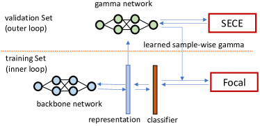
Figure 1: Our proposed approach for regularizing base network towards better calibration with two new components: $\gamma$-Net and SECE . The inner loop optimizes backbone network (e.g., resnet) which uses focal loss as objective function. The $\gamma$-Net in the outer loop takes the extracted second last layer representation of backbone network as input, learns to output sample-wise $\gamma$ for focal loss at a continuous space. The $\gamma$-Net is optimised by using proposed SECE , a Gaussian-kernel based unbiased and differentiable calibration error.

Recently,  Bohdal et al. [2021] proposed to use meta-learning based approach to calibrate deep models. In their formulation the backbone network learns to optimize the regularized cross-entropy loss while a differentiable proxy to calibration error is used to tune the parameters of weight regularizer. Jishnu et al. Mukhoti et al. [2020] found that focal loss can effectively improve calibration and is a good alternative to regularized cross entropy. They also pointed out that the gamma parameter in focal loss plays a crucial role in making this approach effective. They proposed a sample-dependent schedule for gamma in focal loss (FLSD), which showed superior calibration performance as compared to baselines.

Motivated by both meta-calibration Bohdal et al. [2021] and focal loss Lin et al. [2017] with sample-dependent scheduled gamma (FLSD) Mukhoti et al. [2020] in improving model calibration, we introduce an approach that uses a meta network (named as gamma network, i.e. $\gamma$-Net ) to learn a sample-wise $\gamma$ parameter for the focal loss. Our proposed method is presented schematically in Figure 1. Different to FLSD, where a global gamma parameter is scheduled during training, in this work we learn a gamma parameter for each sample. To achieve this, the $\gamma$-Net is optimised using smooth ECE (SECE ), a differentiable surrogate to expected calibration error (ECE) Naeini et al. [2015]. The output of $\gamma$-Net , i.e. the learned $\gamma$ values are then used to optimize the backbone network towards better calibration; pushing network weights and biases to accurately asses predictive confidence while retaining the original predictive performance.

Our contributions can be summarised as follows:

• We propose a $\gamma$-Net , as meta-network to learn sample-wise $\gamma$ for Focal loss at a continuous space, rather than using pre-defined $\gamma$ value.

• We propose a kernel-based ECE estimator SECE , a variation of the kernel density estimate (KDE) approximation Zhang et al. [2020] to smoothly regularize the $\gamma$-Net towards better calibration.

• We empirically show that $\gamma$-Net can effectively calibrate models and SECE provides stable and smooth calibration. Their combination achieves competitive predictive performance and better scores across multiple calibration metrics as compared to baselines.

2 Related Work

Calibration of ML models of using Platt scaling Platt et al. [1999] and Isotonic Regression Zadrozny and Elkan [2002] have showed significant improvements for SVMs and decision trees. With the advent of neural networks, Niculescu-Mizil et al. Niculescu-Mizil and Caruana [2005a] showed those methods can produce well-calibrated probabilities even without any dedicated modifications. Recently, Huang et al. [2016], Zhai et al. [2021] have performed deeper study on this aspect to accurately classify examples. Guo et al. Guo et al. [2017] and Mukhoti et al. Mukhoti et al. [2020] have shown that while modern NNs are noticeably more accurate but poorly calibrated due to negative log likelihood (NLL) overfitting. Minderer et alMinderer et al. [2021] revisited this problem and found that architectures with large size have a larger effect on calibration but nevertheless, more accurate models tend to produce less calibrated predictions.

One of the first methods to tackle calibration are post-hoc methods. This includes non-parametric methods such as histogram binning Zadrozny and Elkan [2001], isotonic regression Zadrozny and Elkan [2002] and parametric methods such as Bayesian binning into quantiles (BBQ) and Platt scaling Platt et al. [1999]. Beyond those four, temperature scaling (TS) is a single-parameter extension of Platt scaling Platt et al. [1999] and the most recent addition to the offering of post-hoc methods. Recent work has showed that a single parameter TS gives good calibration performance with minimal added computational complexity Guo et al. [2017], Minderer et al. [2021]. Extensions to temperature scaling include attention-based mechanism to tackle noise in validation data Mozafari et al. [2018] and introduction of variational dropout based on TS to calibrate deep networks.

Calibration is often measured using the expected calibration error (ECE). Minimizing this measure is the main goal of most calibration-promoting approaches and can be achieved by directly optimising the ECE or its proxy. Kumar et al. Kumar et al. [2018] developed a differentiable equivalent of ECE, the Maximum Mean Calibration Error, which can be optimized directly to train calibrated models. Similarly, Bohdal et al. Bohdal et al. [2021] use a meta-training approach first presented by Luketina et al. Luketina et al. [2015] to train a model that minimizes the differentiable ECE (DECE) to find the optimal parameters of the L2 regualarizers.

Finally, there are methods that do not include the calibration objective explicitly but rather implicitly guide the training towards better calibration performance. Focal loss Lin et al. [2017] which acts as a maximum entropy regularizer Mukhoti et al. [2020] promoting calibration. Label smoothing Müller et al. [2019] mitigates miscalibration by softening hard label with an introduced smoothing modifier in standard loss function (e.g., cross-entropy), while Mix-up training Thulasidasan et al. [2019] extends mixup Zhang et al. [2018] to generate synthetic sample during model training by combining two random elements from the dataset.

In this work, we follow the recent meta-learning based approach and propose to learn a $\gamma$-Net which offers instance-level regularization to base network towards better calibration.

3 Preliminaries

3.1 Model Calibration

Calibration Guo et al. [2017] measures and verifies how the predicted probability estimates the true likelihood of correctness. Assume a model $\mathbf{m}$ trained with dataset $\{\mathbf{x},y\},\mathbf{x}\in\mathcal{X},y\in\mathcal{Y}$. $\mathbf{\hat{p}}$ is the predicted softmax probability. If $\mathbf{m}$ makes 100 independent predictions, each with confidence $p=\arg\max(\mathbf{\hat{p}})=0.9$, ideally, a calibrated $\mathbf{m}$ approximately gives 90 correct predictions. Formally, $\text{accuracy}(\mathbf{m}(D))=\text{confidence}(\mathbf{m}(D))$ if $\mathbf{m}$ is perfectly calibrated on dataset $D$. It is difficult to achieve perfect calibration in practice.

Reliability Diagrams DeGroot and Fienberg [1983], Niculescu-Mizil and Caruana [2005a] visualise whether a model is over- or under-confident by grouping predictions into bins according to their prediction probability. The predictions are grouped into $N$ interval bins (each of of size $1/N$) and the accuracy of samples $y_{i}$ wrt. to the ground truth label $\hat{y}_{i}$ in each bin $b_{n}$ is computed as: $\textrm{acc}(b_{n})=\frac{1}{|b_{n}|}\sum_{i}^{I}\bm{1}(\hat{y}_{i}=y_{i})$, where $i$ indexes all examples that fall into bin $b_{n}$. Let $\hat{p}_{i}$ be the probability for the predicted class $y_{i}$ for $i$-th sample (i.e. the class with highest predicted probability for $i$-th sample), then average confidence is defined as: $\textrm{conf}(b_{n})=\frac{1}{|b_{n}|}\sum_{i}^{I}\hat{p}_{i}$. A model is perfectly calibrated if $\textrm{acc}(b_{n})=\textrm{conf}(b_{n}),\forall n$ and in a diagram the bins would follow the identity function. Any deviation from this represents miscalibration.

Expected Calibration Error (ECE) Naeini et al. [2015]. ECE computes the difference between model accuracy and confidence which, in the general form, can be written as $\mathrm{E}_{\hat{P}}[|\mathbb{P}(\hat{Y}=Y\mid\hat{P}=p)-p|]$ where the expectation is taken over all class probabilities (confidence) $\hat{P}$. ECE in this form is impossible to compute and it is approximated by partitioning data points into bins with similar confidence resulting in a new formulation of $\textsc{ECE}=\sum_{n=1}^{N}\frac{|b_{n}|}{N}|\textrm{acc}(b_{n})-\textrm{conf}(b_{n})|,$ where $N$ is the total number of samples and $b_{n}$ represents a single bin.

Maximum Calibration Error (MCE) Naeini et al. [2015] is particularly important in high-risk applications where reliable confidence measures are absolutely necessary. It measures the worst-case deviation between accuracy and confidence, $\textsc{MCE}=max_{n\in\{1,\dots,N\}}|\textrm{acc}(b_{n})-\textrm{conf}(b_{n})|.$ For a perfectly calibrated model, the ideal ECE and MCE equal to 0. Besides ECE and MCE, we also report Classwise ECE Nixon et al. [2019] and Adaptive ECE Nixon et al. [2019], we describe these metrics in Supplementary Material Section 1.

3.2 Focal Loss

Focal loss Lin et al. [2017] was originally proposed to handle the issue of imbalanced data distribution. For a classification task, the focal loss can be defined as

$$\mathcal{L}^{f}_{\gamma}=-(1-p_{i,y_{i}})^{\gamma}\log p_{i,y_{i}}$$ (1)

where $\gamma$ is a hyper-parameter. Jishnu et al. Mukhoti et al. [2020] found focal loss to be effective at learning better calibrated models as compared to cross-entropy loss. Focal loss can be interpreted as a trade-off between minimizing Kullback–Leibler (KL) divergence and maximizing the entropy, depending on $\gamma$ Mukhoti et al. [2020]:

$$\mathcal{L}_{f}\geq\textsc{KL}(q\parallel p)+\underbrace{\mathbb{H}(q)}_{constant}-\gamma\mathbb{H}(p)$$ (2)

where $p$ is the predictions distribution and $q$ is the one-hot encoded target class. Models trained with this loss learn to have narrow $p$ (high confidence of predictions) due to KL term but not too narrow (avoiding overconfidence) due to entropy regularization term. Original authors provided a principled approach to select the $\gamma$ for focal loss based on Lambert-W function Corless et al. [1996]. Motivated by this, our work proposes to learn a more fine-gained sample-wise $\gamma$ with a meta network.

3.3 Meta-Learning

Model calibration can be formulated as minimizing a multi-component loss objective where the base term is used to optimise predictive performance while a regularizer maintains model calibration  Bohdal et al. [2021], Lin et al. [2017]. Tuning the hyper-parameters of the regularizer can be an a difficult process when conventional methods are used Li et al. [2016], Snoek et al. [2012], Falkner et al. [2018]. In this work, we adopt the meta learning approach Luketina et al. [2015]. At each training iteration, model takes a mini-batch from the training dataset $D_{train}$ and the validation dataset $D_{val}$ to optimise

$$\arg\min_{\theta,\phi} \leavevmode\nobreak\ \mathcal{L}(\theta,\phi,D_{train},D_{val})$$ (3)

$$=\mathcal{L}_{FL_{\gamma}}(\theta,D_{train})+\mathcal{L}_{SECE}(\phi,D_{val})$$ (4)

First, the base loss function $\mathcal{L}_{FL_{\gamma}}$ is used to optimize the parameter of the backbone model $\theta$ on $D_{train}$, note that the $\gamma$ parameter for this step is predicted by $\gamma$-Net . Following that, the validation mini batch $D_{val}$ is used to optimize the parameters of the meta-network ($\gamma$-Net ) $\phi$ using a validation loss $\mathcal{L}_{SECE}$. The validation loss is a function of the backbone model outputs and does not depend on $\gamma$-Net directly. The dependence between validation loss and parameters of the meta-network is mediated via the parameters of the backbone model as discussed by Luketina et al. [2015].

4 Methods

This section introduces the two components of our approach: the $\gamma$-Net learns to parameterise the focal loss and the SECE provides differentiability to $\gamma$-Net towards calibration optimization.

4.1 $\gamma$-Net: Learning Sample-Wise Gamma for Focal Loss

Sample-dependent $\gamma$ value for focal loss showed it effectiveness of calibrating deep neural networks Mukhoti et al. [2020]. In this work, instead of scheduling $\gamma$ value based on Lambert-W function Corless et al. [1996]. We propose to learn a more fine-grained and local $\gamma$ value, i.e., each sample has an individual $\gamma$, at a continuous space. Formally, $\gamma$-Net takes the representations from the second last layer of a backbone network (i.e. ResNet He et al. [2016]. Let $\mathbf{x}\in\mathbb{R}^{b\times d}$ ($b$: batch size, $d$: hidden dimension) be the extracted representation, $\mathbf{A}\in\mathbb{R}^{d\times k}$ be a $k$-head self-attention matrix that followed by a liner layer with parameters $\mathbf{W}\in\mathbb{R}^{d\times 1}$. The $\gamma$-Net transforms the representation to sample-wise $\gamma$:

$$\mathbf{a} =\mathbf{x}\cdot\mathbf{A},\leavevmode\nobreak\ \in\mathbb{R}^{b\times k},\leavevmode\nobreak\ \mathbf{p}=\textsc{Softmax}(\mathbf{a}),\leavevmode\nobreak\ \in\mathbb{R}^{b\times k}$$ (5)

$$\tilde{\mathbf{x}} =\mathbf{p}\cdot\mathbf{A}^{\top},\leavevmode\nobreak\ \in\mathbb{R}^{b\times d},\leavevmode\nobreak\ \leavevmode\nobreak\ \gamma=\left|\tilde{\mathbf{x}}\cdot\mathbf{W}\right|/\tau,\leavevmode\nobreak\ \in\mathbb{R}^{b\times 1}$$ (6)

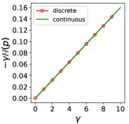
Figure 2: The entropy of predicted probability$-\mathbb{H}(p)$ computed with discrete and continuous $\gamma$ values based on a synthetic set with 1000 samples on a 10-way classification task ($L=10$).

Here we use $|\cdot|$ to ensure the $\gamma$ to be positive values and tune the temperature $\tau=0.01$ for the sake of simplicity. This is similar to the temperature setups as in meta-calibration Bohdal et al. [2021]. Those operations result in a set of sample-wise $\gamma$ in focal loss $\mathcal{L}_{r}^{f}$. Noted that,$f_{\gamma}(\gamma_{i}|x_{i}),x_{i}\in D$ is learned at a continuous space, rather than predefined discrete values as in Focal Loss Lin et al. [2017] and scheduled discrete value depending on samples over batches in FLSD Mukhoti et al. [2020]. As presented in Corollary 1, the learned $\gamma$ at a continuous space provides smooth calibration. Figure 2 further presents the entropy of probability $-\mathbb{H}(p)$, based on smooth and continuous $\gamma$ illustrating how switching from discreet to continuous gamma makes the regularizer smooth  Pereyra et al. [2017].

Corollary 1.

Learning $\gamma$ at a continuous space gives smooth calibration.

Proof.

With eq.(2) Mukhoti et al. [2020], the negative entropy of predictions component of the focal loss $-\gamma\mathbb{H}(p)$ calibrates models by maximising entropy depending on the $\gamma$ hyper-parameter. Given conditions (a) $\gamma$ is continuous and positive and (b) $0\leq-\mathbb{H}(p)\leq-\hat{p}\log(\hat{p}),\sum_{l}^{L}p_{l}=1$ where $p$ is the predicted class probability, $\hat{p}=\frac{1}{L}$ is a uniform distribution that maximizes entropy and $L$ is the number of classes (maximum entropy principle Guiasu and Shenitzer [1985]). The $-\gamma\mathbb{H}(p)$ is continuous and positive. ∎

Practical Considerations To ensure $\gamma\geq 0$, we could apply operations based on min-max scaling or activation functions such as sigmoid, relu and softplus. However, our experimental evidences shows that the formulation presented in Equation 6 performs better across datasets.

4.2 SECE : Smooth Expected Calibration Error

Conventional calibration measurement via ECE discussed in Section 3.1, is computed over discrete bins by finding the accuracy and the confidence of examples in each interval. However, this approach is highly dependant on different settings of bin-edges and the number of bins, making it a biased estimator of the true value Minderer et al. [2021].

The issue of bin-based ECE can be traced back to the discrete decision of binning samples Minderer et al. [2021]. The larger bin numbers, the lesser information retained. Small bins lead to inaccurate measurements of accuracy. For instance, in single example bins, the confidence is well defined but the accuracy in that interval of model confidences is more difficult to assess accurately from a single point. Using the binary accuracy of a single example leads us to the brier score Brier et al. [1950] which has been shown to not be a perfect measure of calibration.

To find a good representation of accuracy inside the single-example bin (representing a small confidence interval), we leverage the accuracy of other points in the vicinity of the single chosen example weighted by their distance in the confidence space. Concretely, we can write the soft estimate of a single-example bin accuracy as

$$\text{SACC\leavevmode\nobreak\ }(b_{i})=\sum_{j}^{M}\pi(x_{i})K(z_{i},z_{j})$$ (7)

$$K\left(x_{i},x_{j}^{\prime}\right)=\exp\left(-\frac{\left\|x_{i}-x_{j}^{\prime}\right\|^{2}}{2h^{2}}\right)$$ (8)

where $b_{i}$ is the bin housing example $x_{i}$ and $K(\cdot,\cdot)$ is a chosen distance measure, for example a Gaussian kernel and $h$ is bandwidth, $z_{i}$ and $\pi(x_{i})$ are the confidence and accuracy of $i^{th}$ example. As in meta-calibration Bohdal et al. [2021], we use the all-pairs approach Qin et al. [2010] to ensure differentiability. Having good measures of soft accuracy and confidence for each single-example bin, we can write the updated ECE metric as soft-ECE in the form

$$\text{SECE\leavevmode\nobreak\ }=\frac{1}{M}\sum_{i}^{M}|\textrm{SACC\leavevmode\nobreak\ }(i)-\textrm{conf}(i)|,$$ (9)

where $i$ represents a single example and $M$ is the number of examples. The new formulation is (1) differentiable as long as the kernel we use is differentiable and (2) enables smooth control over how accuracy over a confidence bin is computed via tuning the kernel parameters. Regarding (2), choosing a dirac-delta function recovers the original brier score while choosing a broader kernel enables a smooth approximation of accuracy over all confidence values.

Connection to KDE-based ECE Estimator Zhang et al. [2020] present a KDE-based ECE Estimator relying on kernel density estimation to approximate the desired metric. Canonically, ECE is computed as an integral over the confidence space as

$$\hat{\operatorname{ECE}}^{d}=\int\|z-\hat{\pi}(z)\|_{d}^{d}\hat{p}(z)dz$$ (10)

where $z=\{z_{1},z_{2},...,z_{L}\}$ denotes model confidence distribution over $L$ classes, $\|\cdot\|_{d}^{d}$ denotes the $d^{th}$ power of the $\ell_{d}$ norm, and $\hat{p}(z)$ represents the marginal density function of model’s confidence on a given dataset. The $\hat{p}(z)$ and $\hat{\pi}(z)$ are approximated using kernel density estimation. We argue that SECE is a special instance with $d=1$ of $\hat{\operatorname{ECE}}^{d}$ and estimate ECE with max probability $z_{t},t=\arg\max\{z_{1},z_{2},...,z_{L}\}$ for a single instance. And $\operatorname{SECE\leavevmode\nobreak\ }$ is an upper bound of $\hat{\operatorname{ECE}}^{1}$:

$$\hat{\operatorname{ECE}} =\int\left|z-\hat{\pi}(z)\right|\hat{p}(z)dz$$ (11)

$$=\int\left|z_{l}-\hat{\pi}(z_{l})\right|\hat{p}(z_{l})dz_{l}\int\left|z_{t}-\hat{\pi}(z_{t})\right|\hat{p}(z_{t})dz_{t}$$ (12)

$$\leq\int\left|z_{t}-\hat{\pi}(z_{t})\right|\hat{p}(z_{t})dz_{t}=\operatorname{SECE\leavevmode\nobreak\ }$$ (13)

with $l=[1,L],l\neq t$ and density functions:

$$\hat{p}(z_{t})=\frac{h^{-L}}{M}\sum_{i=1}^{M}K\left(z_{t},z_{i}\right),$$ (14)

$$\hat{\pi_{t}}(z_{t})=\frac{\sum_{i=1}^{M}\pi(i)K\left(z_{t},z_{i}\right)}{\sum_{i=1}^{M}K\left(z_{t},z_{i}\right)},$$ (15)

where $h$ is the kernel width and $\pi(i)$ represents the binary accuracy of point $i$. The $p(z_{t})$ is a mixture of dirac deltas centered on confidence predicted for individual points in the dataset (used to approximate ECE). Replacing binary accuracy with accuracy computed using all-pairs approach Qin et al. [2010] result in SECE , which is differentiable and can be computed efficiently for smaller batches of data since the integral is replaced with a sum over all examples in a batch.

Presented changes do not invalidate the analysis of the $\hat{\operatorname{ECE}}$ as an unbiased estimator of ECE as the all-pairs accuracy is an unbiased estimator of accuracy and the details of the $p(z)$ distribution are not used in the derivation beyond setting the bounds. As a result, the analysis described in Zhang et al. [2020] to show their KDE-based approximation to ECE is unbiased can be re-used to show the same property for SECE.

Methods	Error	NLL	ECE	MCE	ACE	Classwise ECE
CIFAR 10
CE	4.812 $\pm$ 0.122	0.335 $\pm$ 0.01	4.056 $\pm$ 0.092	33.932 $\pm$ 5.433	4.022 $\pm$ 0.136	0.848 $\pm$ 0.023
CE (TS)	4.812 $\pm$ 0.122	0.211 $\pm$ 0.005	3.083 $\pm$ 0.140	26.695 $\pm$ 2.959	3.046 $\pm$ 0.157	0.656 $\pm$ 0.022
Focal	4.874 $\pm$ 0.100	0.207 $\pm$ 0.005	3.193 $\pm$ 0.104	28.034 $\pm$ 5.702	3.174 $\pm$ 0.098	0.690 $\pm$ 0.018
FLSD	4.916 $\pm$ 0.074	0.211 $\pm$ 0.005	6.904 $\pm$ 0.462	19.246 $\pm$ 11.071	6.805 $\pm$ 0.446	1.465 $\pm$ 0.088
LS (0.05)	4.744 $\pm$ 0.126	0.232 $\pm$ 0.003	2.900 $\pm$ 0.085	24.860 $\pm$ 8.599	3.985 $\pm$ 0.154	0.727 $\pm$ 0.009
Mixup($\alpha$=1.0)	4.126 $\pm$ 0.068	0.273 $\pm$ 0.033	12.863 $\pm$ 3.2	20.739 $\pm$ 4.205	12.833 $\pm$ 3.161	2.678 $\pm$ 0.615
MMCE	4.808 $\pm$ 0.082	0.333 $\pm$ 0.012	4.027 $\pm$ 0.082	41.647 $\pm$ 10.275	4.013 $\pm$ 0.091	0.845 $\pm$ 0.014
CE-DECE	5.194 $\pm$ 0.161	0.301 $\pm$ 0.038	4.106 $\pm$ 0.402	41.346 $\pm$ 13.325	4.088 $\pm$ 0.395	0.868 $\pm$ 0.074
CE-SECE	5.222 $\pm$ 0.168	0.289 $\pm$ 0.027	4.062 $\pm$ 0.241	50.81 $\pm$ 21.705	4.049 $\pm$ 0.251	0.852 $\pm$ 0.040
FLγ-DECE	5.434 $\pm$ 0.095	0.193 $\pm$ 0.009	2.257 $\pm$ 0.787	56.633 $\pm$ 23.856	2.396 $\pm$ 0.669	0.557 $\pm$ 0.165
FLγ-SECE	5.428 $\pm$ 0.144	0.193 $\pm$ 0.010	2.138 $\pm$ 0.819	22.725 $\pm$ 5.756	2.357 $\pm$ 0.541	0.556 $\pm$ 0.165
CIFAR 100
CE	22.570 $\pm$ 0.438	0.997 $\pm$ 0.014	8.380 $\pm$ 0.336	23.250 $\pm$ 2.436	8.347 $\pm$ 0.344	0.233 $\pm$ 0.006
CE (TS)	22.570 $\pm$ 0.438	0.959 $\pm$ 0.008	5.388 $\pm$ 0.393	13.454 $\pm$ 2.377	5.360 $\pm$ 0.315	0.208 $\pm$ 0.003
Focal	22.498 $\pm$ 0.214	0.900 $\pm$ 0.007	5.044 $\pm$ 0.203	12.454 $\pm$ 0.893	5.015 $\pm$ 0.207	0.203 $\pm$ 0.004
FLSD	22.656 $\pm$ 0.113	0.876 $\pm$ 0.005	5.956 $\pm$ 0.804	14.716 $\pm$ 1.387	5.958 $\pm$ 0.802	0.241 $\pm$ 0.008
LS (0.05)	21.810 $\pm$ 0.172	1.070 $\pm$ 0.011	8.108 $\pm$ 0.346	20.268 $\pm$ 1.536	8.106 $\pm$ 0.346	0.272 $\pm$ 0.006
Mixup($\alpha$=1.0)	21.210 $\pm$ 0.227	0.917 $\pm$ 0.017	9.716 $\pm$ 0.754	16.01 $\pm$ 1.335	9.722 $\pm$ 0.74	0.315 $\pm$ 0.011
MMCE	22.490 $\pm$ 0.143	1.021 $\pm$ 0.007	8.713 $\pm$ 0.245	23.565 $\pm$ 1.141	8.670 $\pm$ 0.305	0.238 $\pm$ 0.004
CE-DECE	23.406 $\pm$ 0.323	1.148 $\pm$ 0.006	7.309 $\pm$ 0.245	22.565 $\pm$ 1.446	7.253 $\pm$ 0.315	0.241 $\pm$ 0.002
CE-SECE	23.448 $\pm$ 0.302	1.153 $\pm$ 0.015	7.668 $\pm$ 0.330	24.261 $\pm$ 1.614	7.609 $\pm$ 0.295	0.244 $\pm$ 0.002
FLγ-DECE	23.712 $\pm$ 0.204	0.888 $\pm$ 0.009	1.879 $\pm$ 0.440	8.271 $\pm$ 2.651	1.838 $\pm$ 0.371	0.195 $\pm$ 0.005
FLγ-SECE	23.686 $\pm$ 0.377	0.877 $\pm$ 0.004	1.940 $\pm$ 0.365	7.480 $\pm$ 1.867	1.939 $\pm$ 0.379	0.192 $\pm$ 0.006
Tiny-ImageNet
CE	40.110 $\pm$ 0.110	1.838 $\pm$ 0.171	8.059 $\pm$ 1.296	15.73 $\pm$ 1.905	8.006 $\pm$ 1.282	0.154 $\pm$ 0.001
Focal	39.415 $\pm$ 0.625	1.896 $\pm$ 0.009	7.600 $\pm$ 0.309	13.771 $\pm$ 0.897	7.469 $\pm$ 0.301	0.152 $\pm$ 0.002
FLSD	39.705 $\pm$ 0.075	1.904 $\pm$ 0.025	14.501 $\pm$ 1.078	21.528 $\pm$ 2.116	14.501 $\pm$ 1.078	0.202 $\pm$ 0.006
LS (0.1)	39.395 $\pm$ 0.305	2.185 $\pm$ 0.001	16.777 $\pm$ 0.476	29.088 $\pm$ 1.835	16.901 $\pm$ 0.460	0.199 $\pm$ 0.001
Mixup($\alpha$=1.0)	39.890 $\pm$ 0.271	1.932 $\pm$ 0.054	12.133 $\pm$ 2.069	31.440 $\pm$ 0.968	12.028 $\pm$ 2.079	0.193 $\pm$ 0.009
MMCE	40.310 $\pm$ 0.100	1.826 $\pm$ 0.177	8.206 $\pm$ 1.219	16.802 $\pm$ 2.339	8.165 $\pm$ 1.269	0.149 $\pm$ 0.001
CE-DECE	41.350 $\pm$ 0.000	2.228 $\pm$ 0.033	10.694 $\pm$ 0.503	20.888 $\pm$ 0.430	10.553 $\pm$ 0.553	0.160 $\pm$ 0.000
CE-SECE	41.005 $\pm$ 0.145	2.213 $\pm$ 0.058	10.928 $\pm$ 1.125	21.362 $\pm$ 2.526	10.912 $\pm$ 1.069	0.157 $\pm$ 0.003
FLγ-DECE	40.625 $\pm$ 0.095	1.826 $\pm$ 0.007	5.944 $\pm$ 1.090	11.542 $\pm$ 1.990	6.077 $\pm$ 1.095	0.155 $\pm$ 0.007
FLγ-SECE	40.850 $\pm$ 0.140	1.829 $\pm$ 0.005	5.794 $\pm$ 0.756	11.477 $\pm$ 1.563	5.848 $\pm$ 0.751	0.156 $\pm$ 0.005

Table 1: The predictive (test error) and calibration performance of different methods on CIFAR10 (Top), CIFAR100 (Middle) and Tiny-ImageNet (Bottom). The best scores are bold. The mean and standard deviation numbers are reported by averaging 5 runs with random seeds. As an alternative calibration method, our approach in general exhibits better calibration while retains competitive predictive performance as compared to conventional as well as meta-learning baselines.

4.3 Optimising $\gamma$-Net with SECE 

As the probability calibration via maximising entropy is performed at a continuous space, we argue that SECE is an efficient learning objective for optimising $\gamma$-Net in providing calibration regularization to base network trained with focal loss (see empirical results in 5.2.1).

Under the umbrella of meta-learning, two sets of parameters are learned simultaneously: $\theta$, the parameters of base network $f^{c}$, as well as the $\phi$, the parameters of $\gamma$-Net denoted as $f^{\gamma}$. The former, $f^{c}$, is used to classify each new example into appropriate classes and the latter, $f^{\gamma}$, is applied to find the optimal value of the focal loss parameter $\gamma$ for each training example. Algorithm 1 in Supplementary Material describes the learning procedures.

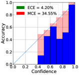
(a) CE (4.94%)

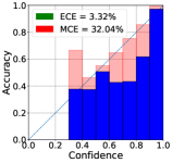
(b) CE (TS) (4.94%)

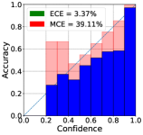
(c) Focal (5.01%)

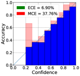
(d) FLSD(5.02%)

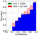
(e) LS-0.05 (4.67%)

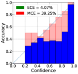
(f) MMCE (4.83%)

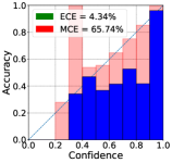
(g) CE-DECE(5.19%)

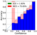
(h) FL_γ-DECE(5.36%)

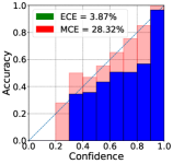
(i) CE-SECE (5.06%)

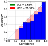
(j) FL_γ+SECE(5.38%)

Figure 3: The reliability diagram plots for models on CIFAR10 test set. The ($\cdot$) presents test error. The diagonal dash line presents perfect calibration. The red bar presents the gap between the observed accuracy and the desired accuracy of the perfectly calibrated model (diagonal) - it is positive if the observed accuracy is lower and negative otherwise. The model from the 5^th run is used.

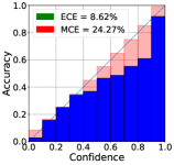
(a) CE (22.41%)

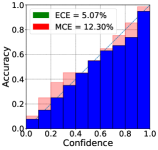
(b) CE (TS) (22.41%)

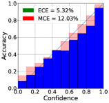
(c) Focal (22.53%)

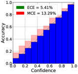
(d) FLSD(22.72%)

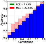
(e) LS-0.05 (21.56%)

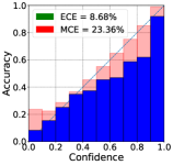
(f) MMCE (22.30%)

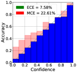
(g) CE-DECE(23.05%)

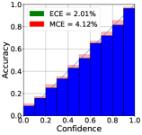
(h) FL_γ-DECE(24.04%)

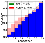
(i) CE-SECE(23.58%)

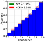
(j) FL_γ-SECE(23.78%)

Figure 4: The reliability diagram plots for models on CIFAR100 test set.

5 Experiments

We conduct experiments to accomplish following objectives:(1) examine both predictive and calibration performance of proposed method;(2) observe the calibration behaviors of proposed method during training;(3) empirically evaluate learned $\gamma$ values for Focal loss and the robustness of different methods in terms of number of bins.

5.1 Implementation Details

We implemented our methods by adapting and extending the code from Meta-Calibration Bohdal et al. [2021] with Pytorch Paszke et al. [2019]. For all experiments we use their default settings. We run each experiments for 5 repetitions with different random seeds. We conducted our experiments on CIFAR10 and CIFAR100 (in Bohdal et al. [2021]) as well as Tiny-ImageNet Ya Le [2015]; For meta-learning, we split the training set into 8:1:1 as training/val/meta-val, the original test sets are untouched. The experimental pipeline for all three datasets is identical. The models are trained with SGD (learning rate 0.1, momentum 0.9, weight decay 0.0005) for up to 350 epochs. The learning rate is decreased at 150 and 250 epochs by a factor of 10. The model selection is based on the best validation error.

The $\gamma$-Net is implemented with a multi-head attention layer with $k$ heads and a fully-connected layer. The $k$ is set to the number of categories. The hidden dim is set to 512, the temperature $\tau$ is fixed at 0.01. For SECE , we used the Gaussian kernel with bandwidth of 0.01 for both dataset. We initialize $\gamma=1.0$. At inference stage, the meta network will not present except our ablation study on learned $\gamma$ values in Section 5.2.2.

Baselines. We compare our method with standard cross-entropy (CE), cross-entropy with post-hoc temperature scaling (TS) Platt et al. [1999], Focal loss with standard gamma value (Focal), $\gamma=1$ Lin et al. [2017], Focal Loss with scheduled gamma (FLSD) Mukhoti et al. [2020], MMCE (Maximum Mean Calibration Error) Kumar et al. [2018] and Label Smoothing with smooth factor 0.05 (LS-0.05) or (LS-0.1) Müller et al. [2019] and Mix-Up ($\alpha=1.0$) Thulasidasan et al. [2019]. In meta-learning setting, we include CE-DECE (meta-calibrationBohdal et al. [2021] for learning unit-wise weight regularization), which is also used as meta-learning baseline, CE-SECE, FL_γ-DECE, focal loss with learnable sample-wise $\gamma$ and FL_γ-DECE. Note that, we excluded the line of work using uncertainty estimation methods for calibration Gawlikowski et al. [2021], for instance, deep ensembles Lakshminarayanan et al. [2017], MC-dropout Gal and Ghahramani [2016], Bayesian Methods  Maddox et al. [2019] etc., those methods usually require performing sampling across multiple inference runs and computational sensitive.

5.2 Results and Discussion

5.2.1 Predictive and Calibration Performance

Table 1 presents the performance comparison across approaches. Temperature Scaling (TS) can effectively reduce the errors on calibration metrics as compared to uncalibrated CE models (baseline). Label smoothing and Mixup achieve the best test errors on datasets but exhibit higher ECE and MCE scores. Focal and FLSD can improve calibration in general but we also observed high MCE score for FLSD. On the other hand, we also found that MMCE exhibits higher calibration errors as compared to baseline, this basically aligns with the findings from Bohdal et al. Bohdal et al. [2021].

Among compared methods, our method FL_γ-SECE achieves considerably lower errors on calibration metrics. When comparing meta-learning based approaches: CE-DECE (meta-learning baseline), CE-SECE, FL_γ-DECE, FL_γ-SECE. We can see that our method ($\gamma$-Net +SECE ) achieves comparable test error and better scores across calibration metrics. Particularly, it improves ECE by average  4.198% on three detests, in addition, by average 14.37% MCE and  3.917% ACE score respectively.

Figure  3 and Figure  4 illustrate the reliability diagram plots of models on CIFAR10 and CIFAR100 respectively. On CIFAR 10, LS(0.05) exhibits superior performance on both predictive and calibration aspects across non-meta learning approaches. DECE based approach basically gives high MCE score 65.74% and 75.65% for CE-DECE and FL_γ-DECE (though is has low ECE 1.83%). It is shown that $\gamma$-Net based methods achieve better ECE as using SECE meta-loss for optimizing $\gamma$-Net ensures smooth and stable calibrations, and potentially reduces the calibration biases on bins. Similarly on CIFAR100, FL_γ-SECE shows improved ECE and MCE from CE-DECE.

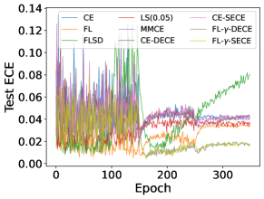
(a)

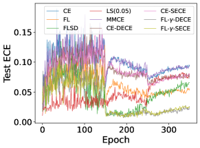
(b)

Figure 5: ECE curves on both test dataset of CIFAR10 (left) and CIFAR100 (right).

Methods	Error	NLL	ECE	MCE	ACE	Classwise ECE
FLγ	5.632 $\pm$ 0.118	0.197 $\pm$ 0.009	2.177 $\pm$ 0.619	46.172 $\pm$ 28.24	2.319 $\pm$ 0.407	0.553 $\pm$ 0.12
FLγ-SECE	5.428 $\pm$ 0.144	0.193 $\pm$ 0.010	2.138 $\pm$ 0.819	22.725 $\pm$ 5.756	2.357 $\pm$ 0.541	0.556 $\pm$ 0.165
FLγ	28.148 $\pm$ 8.127	1.051 $\pm$ 0.278	3.044 $\pm$ 1.542	10.082 $\pm$ 3.441	3.016 $\pm$ 1.511	0.226 $\pm$ 0.063
FLγ-SECE	23.686 $\pm$ 0.377	0.877 $\pm$ 0.004	1.940 $\pm$ 0.365	7.480 $\pm$ 1.867	1.939 $\pm$ 0.379	0.192 $\pm$ 0.006

Table 2: Individual calibration gain from SECE in our method on CIFAR10 (top) and CIFAR100 (bottom).

To observe the learning behavior of models, we plotted the changing curves of test error (included in Supplementary Material Section 3) and test ECE in Figure 8. It is noted that though test error curves show similar behaviors, but the calibration behaviors are quite different across methods. The primary value of $\gamma$-Net with SECE is in the stable and smooth calibration behavior. After the 150^th epoch when the learning rate is decreased by a factor of 10, we can observe that the ECE score starts to increase for all approaches, particularly FLSD (green lines).

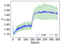
(a) CIFAR10

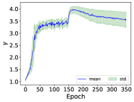
(b) CIFAR100

Figure 6: The mean and standard deviation (std.) of $\gamma$ on test dataset at each epoch. Low std. score indicates samples share similar gamma values, and high std. score indicates more samples have different $\gamma$ values.

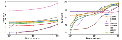
Figure 7: The ECE and MCE scores on CIFAR 10 test dataset with different bin numbers in $[10,20,50,100,200,500,1000]$. Our proposed approach shows better robustness on bin sizes. Similar plot for CIFAR100 is in Figure 2 of Supplementary Material.

5.2.2 Ablation Experiments

We conducted two groups of experiments to inspect the learned $\gamma$ and the ECE/MCE against different binning schemes.

Figure 6 presents the change of $\gamma$ values on test dataset over epochs. At the earlier training stage, the samples $\gamma_{j}$ for $x_{j}\in D_{test}$ have similar values (with low variance) because they are initialized with $\gamma_{i}=1.0$ for $x_{i}\in D_{val}$. The $\gamma$ parameter is observed to have higher standard deviation at the later training stage as $\gamma$-Net learns optimal value for each example in the dataset rather than relying on global values showcasing the flexibility of the network. It is also noted that $\gamma$ is learned in a continuous space, different to the discrete values the pre-defined in Focal Loss Lin et al. [2017] and FLSD Mukhoti et al. [2020].

In Figure 7, we examine the robustness of those methods with different binning schemes by varying the number of bins, which is one of causes of introducing calibration bias Minderer et al. [2021]. It shows that $\gamma$-Net based approaches (FL_γ-DECE and FL_γ-SECE) maintain much lower ECE score when throughout all bin numbers from 10 to 1000 showing the trained based network is robustly calibrated. Furthermore FL_γ-SECE is also able to maintain lower MCE as compared to other methods. Supplementary Material Section 3.2 reports reliability diagrams with large bin numbers.

We further conducted experiments to empirically understand the individual calibration gain from SECE as compared to using learnable $\gamma$ only. Table 2 shows the effectiveness of SECE in our method FL_γ+SECE. With SECE , we can see the improved both predictive and calibration performance.

6 Conclusion

In this work, we presented a meta-learning based approach for learning well calibrated models and shown the benefits of two newly introduced components. Learning a sample-wise $\gamma$ for Focal loss using $\gamma$-Net yields both strong predictive performance and good calibration. Optimising $\gamma$-Net with SECE plays an important role by ensuring stable calibration as compared to baselines; it provides better calibration capability without changing the original networks.

Appendix A Supplementary Material

A.1 Evaluation Metrics

Besides ECE and MCE, we evaluate models on Classwise ECE and Adaptive ECE.

Classwise ECE Nixon et al. [2019]. Classwise ECE extends the bin-based ECE to measure calibration across all the possible classes. In practice, predictions are binned separately for each class and the calibration error is computed at the level of individual class-bins and then averaged. The metric can be formulated as

$$\textsc{CECE}=\sum_{n=1}^{N}\sum_{c=1}^{K}\frac{|b_{n,c}|}{NK}|\textrm{acc}_{c}(b_{n,c})-\textrm{conf}_{c}(b_{n,c})|$$ (16)

where $N$ is the total number of samples, K is the number of classes and $b_{n,c}$ represents a single bin for class $c$. In this formulation, $\textrm{acc}_{c}(b_{n,c})$ represents average binary accuracy for class $c$ over bin $b_{n,c}$ and $\textrm{conf}_{c}(b_{n,c})$ represents average confidence for class $c$ over bin $b_{n,c}$

Adaptive ECE Nixon et al. [2019]. Adaptive ECE further extends the classwise variant of expected calibration error by introducing a new binning strategy which focuses the measurement on the confidence regions with multiple predictions and. Concretely Adaptive ECE (ACE) spaces the bin intervals such that each contains an equal number of predictions. The metric can be formulated as

$$\textsc{CECE}=\sum_{n=1}^{N}\sum_{c=1}^{K}\frac{1}{NK}|\textrm{acc}_{c}(b_{n,c})-\textrm{conf}_{c}(b_{n,c})|$$ (17)

where the notation follows one from classwise ECE. The importance weighting for each bin is removed since each bin holds the same number of examples.

A.2 Algorithm

Algorithm 1 describes the learning procedures, it relies on the training and validation sets $D_{train}$, $D_{val}$, two networks $f^{c}$ and $f^{\gamma}$ with parameters $\theta$ and $\phi$. The optimization proceeds in an iterative process until both sets are converged. Each iteration starts by sampling a mini-batch of training data $(\mathbf{x}_{i}^{t},\mathbf{y}_{i}^{t})\sim D_{train}$ as well as a mini-batch of validation data $(\mathbf{x}_{i}^{v},\mathbf{y}_{i}^{v})\sim D_{val}$. The training-mini batch is used to find the optimal value of $\gamma$ as $\gamma=f^{\gamma}(\mathbf{x}_{i}^{t})$ and following that, compute the focal loss on the output of the backbone network $f^{c}$. The gradient of the loss $\mathcal{L}^{f}_{\gamma}({f^{c}(\mathbf{x}_{i}^{t}),\mathbf{y}_{i}^{t}})$ is then used to update the parameters of the backbone network $\theta$ using the Adam algorithm Kingma and Ba [2014].

Once the backbone model $f^{c}$ is updated, it is used to compute the value of the auxiliary loss SECE on the validation mini-batch SECE $({f^{c}(\mathbf{x}_{i}^{v}),\mathbf{y}_{i}^{v}})$. The auxiliary SECE loss is a differentiable proxy of the true expected calibration error and can be minimized w.r.t. $\phi$ to find the optimal parameters of $\gamma$-Net . It is important to note that SECE is computed based on the outputs of $f^{c}(\mathbf{x}_{i}^{v})$ and the only dependence on $\gamma$ is an indirect one based on the updates of $\theta$ as discussed in Section 2.3.

1

Input: $f^{c}$ and $f^{\gamma}$ with initialized $\theta$ and $\phi$

Output: Optimized $\theta$ and $\phi$

Data: Training and validation sets: $D_{train},D_{val}$

2 while $\theta$ not converged do

3       $(\mathbf{x}_{i}^{t},\mathbf{y}_{i}^{t})\sim D_{train};\leavevmode\nobreak\ \leavevmode\nobreak\ \leavevmode\nobreak\ (\mathbf{x}_{i}^{v},\mathbf{y}_{i}^{v})\sim D_{val}$; # Sample a mini-batch from both datasets

4       $\gamma_{i}=f^{\gamma}(\mathbf{x}_{i}^{t})$; # learning sample-wise $\gamma_{i}$;

5       $\mathcal{L}^{f}_{\gamma}=\mathcal{L}^{f}_{\gamma}({f^{c}(\mathbf{x}_{i}^{t}),\mathbf{y}_{i}^{t}})$: # Compute training loss based on $\gamma$

6       $\theta:=\theta-\eta\nabla_{\theta}\mathcal{L}^{f}_{\gamma}$: # Update parameters of $f^{c}$ using training loss gradient

7       $SECE\leavevmode\nobreak\ =SECE\leavevmode\nobreak\ ({f^{c}(\mathbf{x}_{i}^{v}),\mathbf{y}_{i}^{v}})$: # Compute SECE auxiliary loss using validation batch

8       $\phi:=\phi-\eta_{\phi}\nabla_{\phi}SECE\leavevmode\nobreak\$: # Update parameters of $f^{\gamma}$ using SECE gradient

9      

Algorithm 1 Meta optimization with $\gamma$-Net and SECE

A.3 Additional Experiments

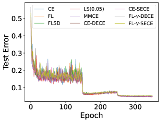
(a) CIFAR10 (Error)

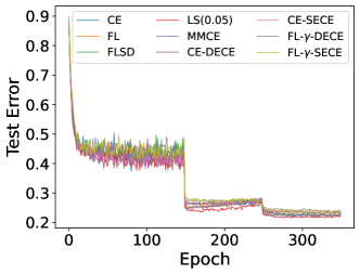
(b) CIFAR100 (Error)

Figure 8: Test error on both test datasets.

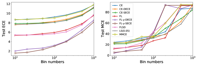
Figure 9: The ECE and MCE scores on CIFAR 100 test dataset with different bin numbers in $[10,20,50,100,200,500,1000]$. Our proposed approach shows better robustness on bin sizes.

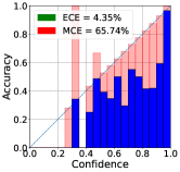
(a) CE-DECE

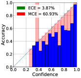
(b) CE-SECE

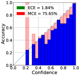
(c) FL_γ-DECE

(d) FL_γ+SECE

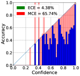
(e) CE-DECE

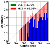
(f) CE-SECE

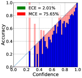
(g) FL_γ-DECE

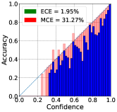
(h) FL_γ+SECE

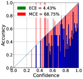
(i) CE-DECE

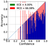
(j) CE-SECE

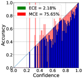
(k) FL_γ-DECE

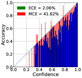
(l) FL_γ+SECE

Figure 10: The reliability diagram plots for models on CIFAR10 with large bin numbers (top to bottom: 20, 50, 100). The diagonal dash line presents perfect calibration, the red bar presents the gap to perfect calibration on each bin. The model from the 5^th run is used.

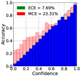
(a) CE-DECE

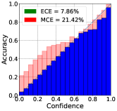
(b) CE-SECE

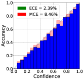
(c) FL_γ-DECE

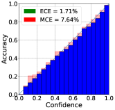
(d) FL_γ+SECE

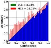
(e) CE-DECE

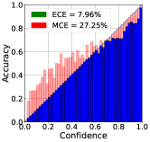
(f) CE-SECE

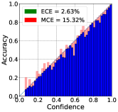
(g) FL_γ-DECE

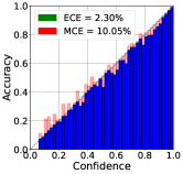
(h) FL_γ+SECE

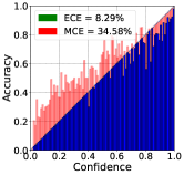
(i) CE-DECE

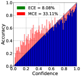
(j) CE-SECE

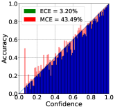
(k) FL_γ-DECE

(l) FL_γ+SECE

Figure 11: The reliability diagram plots for models on CIFAR100 with large bin numbers (top to bottom: 20, 50, 100). The diagonal dash line presents perfect calibration, the red bar presents the gap to perfect calibration on each bin. The model from the 5^th run is used.

A.3.1 Test Error Curves

Figure 8 presents the test error on CIFAR10 and CIFAR100 for compared methods. In general, they exhibit similar behaviour.

A.3.2 Reliability Plots

In Figure 10 and 11, we provide the comparison across meta-learning based approach via reliability plots with large bin numbers and corresponding ECE/MCE. FL_γ+SECE is able to maintain lowest ECE and MCE, it shows the robustness to the increased bin numbers.

Figure 9 examines the robustness of those methods with different binning schemes by varying the number of bins. It shows that $\gamma$-Net based approaches (FL_γ-DECE and FL_γ-SECE) maintain much lower ECE score when throughout all bin numbers from 10 to 1000 showing the trained based network is robustly calibrated.

A.3.3 Experiments with DenseNet

We conducted experiments on DenseNet with meta-learning baselines. Table 3 presents the effectiveness of gamma-net based methods, which exhibit better calibration across multiple metrics with comparable predictive performance.

Methods	Error	NLL	ECE	MCE	ACE	CLASSWISE_ECE
CE	5.354 $\pm$ 0.097	0.22 $\pm$ 0.015	3.038 $\pm$ 0.159	33.419 $\pm$ 19.597	3.035 $\pm$ 0.157	0.677 $\pm$ 0.031
CE-DECE	5.85 $\pm$ 0.421	0.236 $\pm$ 0.017	3.245 $\pm$ 0.471	25.062 $\pm$ 2.184	3.24 $\pm$ 0.471	0.723 $\pm$ 0.072
CE-SECE	5.895 $\pm$ 0.271	0.246 $\pm$ 0.032	3.555 $\pm$ 0.428	24.518 $\pm$ 3.613	3.555 $\pm$ 0.425	0.756 $\pm$ 0.083
FLγ-DECE	6.084 $\pm$ 0.188	0.199 $\pm$ 0.012	2.151 $\pm$ 1.499	24.644 $\pm$ 11.227	2.139 $\pm$ 1.457	0.605 $\pm$ 0.201
FLγ-SECE	6.263 $\pm$ 0.266	0.208 $\pm$ 0.021	2.549 $\pm$ 2.233	20.22 $\pm$ 5.235	2.559 $\pm$ 2.217	0.672 $\pm$ 0.355

Table 3: DenseNet (100 layers) on CIFAR10 with meta-learning based methods, 5 repetitions. gamma-net based methods exhibit better calibration across multiple metrics (NLL, ECE, ACE, CLASSWISE_ECE) while maintain competitive test error.

References

- Bohdal et al. [2021] Ondrej Bohdal, Yongxin Yang, and Timothy Hospedales. Meta-calibration: Meta-learning of model calibration using differentiable expected calibration error. arXiv preprint arXiv:2106.09613, 2021.
- Bojarski et al. [2016] Mariusz Bojarski, Davide Del Testa, Daniel Dworakowski, Bernhard Firner, Beat Flepp, Prasoon Goyal, Lawrence D Jackel, Mathew Monfort, Urs Muller, Jiakai Zhang, et al. End to end learning for self-driving cars. arXiv preprint arXiv:1604.07316, 2016.
- Brier et al. [1950] Glenn W Brier et al. Verification of forecasts expressed in terms of probability. Monthly weather review, 78(1):1–3, 1950.
- Caruana et al. [2015] Rich Caruana, Yin Lou, Johannes Gehrke, Paul Koch, Marc Sturm, and Noemie Elhadad. Intelligible models for healthcare: Predicting pneumonia risk and hospital 30-day readmission. In Proceedings of the 21th ACM SIGKDD international conference on knowledge discovery and data mining, pages 1721–1730, 2015.
- Corless et al. [1996] Robert M Corless, Gaston H Gonnet, David EG Hare, David J Jeffrey, and Donald E Knuth. On the lambertw function. Advances in Computational mathematics, 5(1):329–359, 1996.
- DeGroot and Fienberg [1983] Morris DeGroot and Stephen Fienberg. The comparison and evaluation of forecasters. The Statistician, 1983.
- Falkner et al. [2018] Stefan Falkner, Aaron Klein, and Frank Hutter. Bohb: Robust and efficient hyperparameter optimization at scale. 35th International Conference on Machine Learning, ICML 2018, 4:2323–2341, 7 2018. 10.48550/arxiv.1807.01774. URL https://arxiv.org/abs/1807.01774v1.
- Gal and Ghahramani [2016] Yarin Gal and Zoubin Ghahramani. Dropout as a bayesian approximation: Representing model uncertainty in deep learning. In ICML’16, pages 1050–1059. PMLR, 2016.
- Gawlikowski et al. [2021] Jakob Gawlikowski, Cedrique Rovile Njieutcheu Tassi, Mohsin Ali, Jongseok Lee, Matthias Humt, Jianxiang Feng, Anna Kruspe, Rudolph Triebel, Peter Jung, Ribana Roscher, et al. A survey of uncertainty in deep neural networks. arXiv preprint arXiv:2107.03342, 2021.
- Graves et al. [2013] Alex Graves, Abdel-rahman Mohamed, and Geoffrey Hinton. Speech recognition with deep recurrent neural networks. In 2013 IEEE international conference on acoustics, speech and signal processing, pages 6645–6649. Ieee, 2013.
- Guiasu and Shenitzer [1985] Silviu Guiasu and Abe Shenitzer. The principle of maximum entropy. The mathematical intelligencer, 7(1):42–48, 1985.
- Guo et al. [2017] Chuan Guo, Geoff Pleiss, Yu Sun, and Kilian Q Weinberger. On calibration of modern neural networks. In International Conference on Machine Learning, pages 1321–1330. PMLR, 2017.
- He et al. [2016] Kaiming He, Xiangyu Zhang, Shaoqing Ren, and Jian Sun. Deep residual learning for image recognition. In Proceedings of the IEEE conference on computer vision and pattern recognition, pages 770–778, 2016.
- Huang et al. [2016] Gao Huang, Zhuang Liu, Laurens Van Der Maaten, and Kilian Q. Weinberger. Densely connected convolutional networks. Proceedings - 30th IEEE Conference on Computer Vision and Pattern Recognition, CVPR 2017, 2017-January:2261–2269, 8 2016. 10.48550/arxiv.1608.06993. URL https://arxiv.org/abs/1608.06993v5.
- Kingma and Ba [2014] Diederik P Kingma and Jimmy Ba. Adam: A method for stochastic optimization. arXiv preprint arXiv:1412.6980, 2014.
- Krizhevsky et al. [2012] Alex Krizhevsky, Ilya Sutskever, and Geoffrey E Hinton. Imagenet classification with deep convolutional neural networks. Advances in neural information processing systems, 25, 2012.
- Kumar et al. [2018] Aviral Kumar, Sunita Sarawagi, and Ujjwal Jain. Trainable calibration measures for neural networks from kernel mean embeddings. In International Conference on Machine Learning, pages 2805–2814. PMLR, 2018.
- Lakshminarayanan et al. [2017] Balaji Lakshminarayanan, Alexander Pritzel, and Charles Blundell. Simple and scalable predictive uncertainty estimation using deep ensembles. In NeurIPS’17, 2017.
- Li et al. [2016] Lisha Li, Kevin Jamieson, Giulia DeSalvo, Afshin Rostamizadeh, and Ameet Talwalkar. Hyperband: A novel bandit-based approach to hyperparameter optimization. Journal of Machine Learning Research, 18:1–52, 3 2016. ISSN 15337928. 10.48550/arxiv.1603.06560. URL https://arxiv.org/abs/1603.06560v4.
- Lin et al. [2017] Tsung-Yi Lin, Priya Goyal, Ross Girshick, Kaiming He, and Piotr Dollár. Focal loss for dense object detection. In Proceedings of the IEEE international conference on computer vision, pages 2980–2988, 2017.
- Luketina et al. [2015] Jelena Luketina, Mathias Berglund, Klaus Greff, and Tapani Raiko. Scalable gradient-based tuning of continuous regularization hyperparameters. 33rd International Conference on Machine Learning, ICML 2016, 6:4333–4341, 11 2015. 10.48550/arxiv.1511.06727. URL https://arxiv.org/abs/1511.06727v3.
- Maddox et al. [2019] Wesley J Maddox, Pavel Izmailov, Timur Garipov, Dmitry P Vetrov, and Andrew Gordon Wilson. A simple baseline for bayesian uncertainty in deep learning. NeurIPS, 32, 2019.
- Minderer et al. [2021] Matthias Minderer, Josip Djolonga, Rob Romijnders, Frances Hubis, Xiaohua Zhai, Neil Houlsby, Dustin Tran, and Mario Lucic. Revisiting the calibration of modern neural networks. Advances in Neural Information Processing Systems, 34, 2021.
- Mozafari et al. [2018] Azadeh Sadat Mozafari, Hugo Siqueira Gomes, Wilson Leão, Steeven Janny, and Christian Gagné. Attended temperature scaling: A practical approach for calibrating deep neural networks, 2018. URL https://arxiv.org/abs/1810.11586.
- Mukhoti et al. [2020] Jishnu Mukhoti, Viveka Kulharia, Amartya Sanyal, Stuart Golodetz, Philip Torr, and Puneet Dokania. Calibrating deep neural networks using focal loss. Advances in Neural Information Processing Systems, 33:15288–15299, 2020.
- Müller et al. [2019] Rafael Müller, Simon Kornblith, and Geoffrey E Hinton. When does label smoothing help? Advances in neural information processing systems, 32, 2019.
- Naeini et al. [2015] Mahdi Pakdaman Naeini, Gregory F. Cooper, and Milos Hauskrecht. Obtaining well calibrated probabilities using bayesian binning. In Proceedings of the Twenty-Ninth AAAI Conference on Artificial Intelligence (AAAI), 2015.
- Niculescu-Mizil and Caruana [2005a] Alexandru Niculescu-Mizil and Rich Caruana. Predicting Good Probabilities with Supervised Learning. In Proceedings of the 22nd International Conference on Machine Learning (ICML), 2005a.
- Niculescu-Mizil and Caruana [2005b] Alexandru Niculescu-Mizil and Rich Caruana. Predicting good probabilities with supervised learning. In Proceedings of the 22nd international conference on Machine learning, pages 625–632, 2005b.
- Nixon et al. [2019] Jeremy Nixon, Mike Dusenberry, Ghassen Jerfel, Timothy Nguyen, Jeremiah Liu, Linchuan Zhang, and Dustin Tran. Measuring calibration in deep learning, 2019. URL https://arxiv.org/abs/1904.01685.
- Paszke et al. [2019] Adam Paszke, Sam Gross, Francisco Massa, Adam Lerer, James Bradbury, Gregory Chanan, Trevor Killeen, Zeming Lin, Natalia Gimelshein, Luca Antiga, et al. Pytorch: An imperative style, high-performance deep learning library. Advances in neural information processing systems, 32, 2019.
- Pereyra et al. [2017] Gabriel Pereyra, George Tucker, Jan Chorowski, Łukasz Kaiser, and Geoffrey Hinton. Regularizing neural networks by penalizing confident output distributions. arXiv preprint arXiv:1701.06548, 2017.
- Platt et al. [1999] John Platt et al. Probabilistic outputs for support vector machines and comparisons to regularized likelihood methods. Advances in large margin classifiers, 10(3):61–74, 1999.
- Qin et al. [2010] Tao Qin, Tie-Yan Liu, and Hang Li. A general approximation framework for direct optimization of information retrieval measures. Inf. Retr., 13(4):375–397, aug 2010. ISSN 1386-4564. 10.1007/s10791-009-9124-x. URL https://doi.org/10.1007/s10791-009-9124-x.
- Snoek et al. [2012] Jasper Snoek, Hugo Larochelle, and Ryan P Adams. Practical bayesian optimization of machine learning algorithms. Adv. Neural Inf. Process. Syst. 25, pages 1–9, 2012. ISSN 10495258. 2012arXiv1206.2944S. URL https://arxiv.org/pdf/1206.2944.pdf.
- Thulasidasan et al. [2019] Sunil Thulasidasan, Gopinath Chennupati, Jeff A Bilmes, Tanmoy Bhattacharya, and Sarah Michalak. On mixup training: Improved calibration and predictive uncertainty for deep neural networks. Advances in Neural Information Processing Systems, 32, 2019.
- Vaswani et al. [2017] Ashish Vaswani, Noam Shazeer, Niki Parmar, Jakob Uszkoreit, Llion Jones, Aidan N Gomez, Łukasz Kaiser, and Illia Polosukhin. Attention is all you need. Advances in neural information processing systems, 30, 2017.
- Ya Le [2015] Xuan Yang Ya Le. Tiny imagenet visual recognition challenge, 2015. URL http://vision.stanford.edu/teaching/cs231n/reports/2015/pdfs/yle_project.pdf.
- Zadrozny and Elkan [2001] Bianca Zadrozny and Charles Elkan. Obtaining calibrated probability estimates from decision trees and naive Bayesian classifiers. In Proceedings of the International Conference on Machine Learning (ICML), pages 609–616. Citeseer, 2001.
- Zadrozny and Elkan [2002] Bianca Zadrozny and Charles Elkan. Transforming classifier scores into accurate multiclass probability estimates. In Proceedings of the eighth ACM SIGKDD international conference on Knowledge discovery and data mining, pages 694–699. ACM, 2002.
- Zhai et al. [2021] Xiaohua Zhai, Alexander Kolesnikov, Neil Houlsby, and Lucas Beyer. Scaling vision transformers. 6 2021. 10.48550/arxiv.2106.04560. URL https://arxiv.org/abs/2106.04560v1.
- Zhang et al. [2018] Hongyi Zhang, Moustapha Cisse, Yann N Dauphin, and David Lopez-Paz. mixup: Beyond empirical risk minimization. In International Conference on Learning Representations, 2018.
- Zhang et al. [2020] Jize Zhang, Bhavya Kailkhura, and T. Yong-Jin Han. Mix-n-match: Ensemble and compositional methods for uncertainty calibration in deep learning, 2020. URL https://arxiv.org/abs/2003.07329.