An End-to-End Framework For Universal Lesion Detection With Missing Annotations

Abstract

Fully annotated large-scale medical image datasets are highly valuable. However, because labeling medical images is tedious and requires specialized knowledge, the large-scale datasets available often have missing annotation issues. For instance, DeepLesion, a large-scale CT image dataset with labels for various kinds of lesions, is reported to have a missing annotation rate of 50%. Directly training a lesion detector on it would suffer from false negative supervision caused by unannotated lesions. To address this issue, previous works have used sophisticated multi-stage strategies to switch between lesion mining and detector training. In this work, we present a novel end-to-end framework for mining unlabeled lesions while simultaneously training the detector. Our framework follows the teacher-student paradigm. In each iteration, the teacher model infers the input data and creates a set of predictions. High-confidence predictions are combined with partially-labeled ground truth for training the student model. On the DeepLesion dataset, using the original partially labeled training set, our model can outperform all other more complicated methods and surpass the previous best method by 2.3% on average sensitivity and 2.7% on average precision, achieving state-of-the-art universal lesion detection results.

I Introduction

Universal lesion detectors (ULDs) [1, 2], which aim to discover various types of lesions in multiple organs on radiological images, fit the daily clinical need of general radiologists and thus have significant clinical values. Due to the success of deep learning in computer vision, most ULDs are deep convolutional neural networks (DCNNs), which require a large-scale annotated image dataset to train. Unlike labeling natural images, annotating medical images is costly and requires extensive domain knowledge [3]. The various appearances of lesions on medical images make it even more challenging to annotate all lesions thoroughly. For instance, the large-scale CT image dataset with RECIST annotations [4] for various kinds of lesions, namely DeepLesion, is reported to have 50% lesions unlabeled (see Fig. 1).

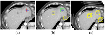
Figure 1: Annotations in DeepLesion dataset. (a) The original RECIST annotation. (b) The RECIST generated bounding box is indicated in green, and two missing annotations are shown in yellow. (c) There is no lesion depth information, therefore the 3D bounding boxes are unavailable.

If we train a ULD on DeepLesion, those unlabeled lesions will be probably misinterpreted as the background, resulting in false negative supervision signals and degrading performance in lesion detection. While ULD has been extensively studied in [1, 5, 6, 7, 8], this issue was only recognized by a few recent works [9, 10, 11, 12]. The key to tackling this missing annotation issue is to filter out the false negative samples generated by unlabelled lesions. Based on this idea, current methods can be categorized into two groups: sampling based and pseudo-label based methods. Sampling based methods aim to find reliable background regions that are not unlabelled objects. For instance, overlap-based hard sampling [13] only samples negative box proposals with an overlap larger than 0.1 to any existing ground truth annotations. The soft sampling method [14] re-weights negative regions based on their overlaps and the center distances with annotated instances. While these strategies can reduce the number of false negative samples, they ignore numerous informative areas that include valuable true negatives.

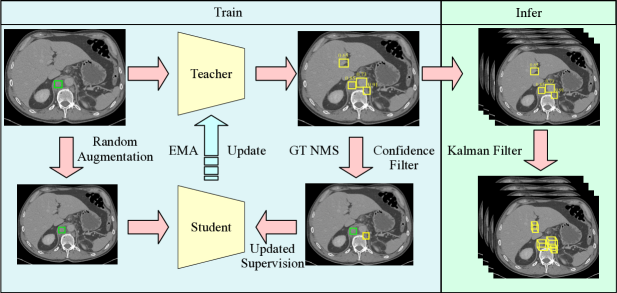
Figure 2: Diagram of the proposed model lesion mining model.

To handle the disadvantages of the sampling based method, pseudo-label based methods consider directly mining unlabelled lesions and using them to guide the model training. Wang et al. [9] advocate using the continuity of multi-slice axial CT images to mine unlabeled lesions. Yan et al. [11] use the knowledge gained from several fully-labeled single-type lesion datasets to assist the ULD training. Cai et al. [10] introduce the lesion-harvester framework, which combines a lesion proposal generator and a lesion proposal classifier to iteratively mine unlabeled lesions and hard negatives for retraining. The previous state-of-the-art method [12] adopts the co-teaching idea and proposes a dual-task model to mutually check the suspicious unlabeled lesions mined by each task. Although these previous pseudo-label based methods improve the overall detection performance, they use complex multi-stage procedures to transition between lesion mining and detector training, which limits their applicability to larger datasets [15]. Furthermore, all these methods require the detectors to be trained to convergence on each stage, while the mined lesions are only updated once. We argue these multi-stage approaches are not optimal, both on the training efficiency and the performance. A better approach may be gradually mining the lesions and bootstrapping the model performance in a more fine-grained process, i.e., in batches, so that the false negative samples can be corrected timely during training.

Based on this concept, we present a model for processing lesion mining on each mini-batch. The performance gained by this change is significant. For instance, on the DeepLesion dataset, in [10] it takes three days to run six iterations for mining the unlabelled lesion, while the average precision (AP) performance only increases from 43.0% to 43.6%. The previous state-of-the-art method [12] achieves the AP performance to 47.5%, but it also relies on extra data processing and fine-tuning steps. In contrast, our method can boost the AP performance to 50.2% by a single end-to-end training process in eight hours.

Specifically, our method adopts the teacher-student framework to simultaneously mine unlabeled lesions and train the detector. For each mini-batch, the teacher branch infers the input data and creates a set of predictions. The high-confidence predictions are considered suspicious lesions and are combined with partially-labeled ground truth to train the student branch. The teacher branch maintains an exponential moving average (EMA) of the student’s parameters and is used as the final output model. The main contributions are summarized as follows: (1)We propose a novel end-to-end framework to address the missing annotation problem in the universal lesion detection task. (2) We systematically compared different policies for dealing with the mined suspicious regions. (3) The proposed framework is highly efficient and achieves the state-of-the-art lesion detection performance on the fully-annotated test set of the DeepLesion dataset.

II Method

Fig. 2 illustrates the overview of our lesion mining and detection model. It follows the teacher-student paradigm [15], consisting of two detection branches with the same structure. The parameters of the student branch are updated by gradient back-propagation under the supervision of the partially labeled ground truth and the mined suspicious lesions from the teacher branch. The teacher branch maintains an exponential moving average (EMA) of the student’s parameters. We use Faster R-CNN [16] as our lesion detector framework.

Given the partially annotated dataset $D_{p}=\{x_{i},y_{i}^{l},y_{i}^{u}\}_{i=1}^{N}$, where $x_{i}$ represents the image and $y_{i}^{l}$ is the available lesion annotations, $y_{i}^{u}$ denotes the missing annotations that are not accessible. For the generation of suspecious lesions, at each mini-batch, the teacher branch first infers the batch inputs $\{x_{i}\}_{i=1}^{N_{b}}$ to give a set of predictions $\{p_{i}^{\rm{T}}\}_{i=1}^{N_{b}}$. Next, the predictions $\{p_{i}^{\rm{T}}\}_{i=1}^{N_{b}}$ are compared with the available ground truth $\{y_{i}^{l}\}_{i=1}^{N_{b}}$ by their intersection over union (IoU) values, we then remove the predictions which have IoU larger than a threshold with any ground truth. For simplicity, we use $P^{\rm{T}}$, $Y^{l}$ and $Y^{u}$ to denote the batch predictions $\{p_{i}^{\rm{T}}\}_{i=1}^{N_{b}}$, available ground truth $\{y^{l}\}_{i=1}^{N_{b}}$ and unlabeled ground truth $\{y^{u}\}_{i=1}^{N_{b}}$. The remaining predictions can be written as $P^{\rm{T}}-P^{\rm{T}}\cap Y^{l}$. This process can be easily implemented using Non-Maximum Suppression (NMS) operation on the predictions and ground truth, we name it as GT NMS operation. Finally, we filter out the predictions with confidence scores lower than threshold $\tau$. The remaining predictions are represented as $P^{m}$ and will be served as mined lesions to feed the student branch.

For the training of the student branch, consider the student branch’s predictions $P^{\rm{S}}=\{p_{i}^{\rm{S}}\}_{i=1}^{N_{b}}$ for the resized batch input images. The detection loss can be summarized as a combination of position classification loss and box regression loss:

$$\mathcal{L}=\mathcal{L}_{cls}(P^{\rm{S}},Y)+\mathcal{L}_{reg}(P^{\rm{S}},Y),$$ (1)

where $Y=Y^{l}+Y^{u}$ is the ground truth. Since the box regression loss $\mathcal{L}_{reg}$ is only computed on each annotated object, it is not influenced by the false negatives issue. However, for the classification loss $\mathcal{L}_{cls}$, it needs to assign each position to one object or background class. Suppose there are $M$ positions, each position represents a prior (anchor) box $b_{i}$ and is assigned to one lesion in $Y$ or background label. For simplicity, we regard all lesions in $Y$ as foreground label. The number of foreground boxes and background boxes are $M^{f}$ and $M^{b}$. The ideal classification loss is:

$$\mathcal{L}_{cls}=\dfrac{M^{f}}{M}\sum_{i=1}^{M^{f}}H(c_{i}^{f},+1)+\dfrac{M^{b}}{M}\sum_{i=1}^{M^{b}}H(c_{i}^{b},-1),$$ (2)

where $c_{i}^{f}$ and $c_{i}^{b}$ represent the model’s output foreground and background probability at each position, $H(t,y)$ indicates the loss between the model’s outputs $t$ and the ground truth $y$.

We can further separate $M^{f}$ into $M^{l}$ and $M^{u}$, corresponding to $Y^{l}$ and $Y^{u}$. Since the $Y^{u}$ are unavailable, the $M^{u}$ will be falsely assigned to background label. Thus the real loss is a biased version:

$$\mathcal{L}_{cls}^{\prime}=\dfrac{M^{l}}{M}\sum_{i=1}^{M^{l}}H(c_{i}^{f},+1)+\dfrac{M^{b}+M^{u}}{M}\sum_{i=1}^{M^{b}+M^{u}}H(c_{i}^{b},-1).$$ (3)

The error is:

$$\mathcal{L}_{cls}^{\prime}-\mathcal{L}_{cls}=-\dfrac{M^{u}}{M}\sum_{i=1}^{M^{u}}H(c_{i}^{f},+1)+\dfrac{M^{u}}{M}\sum_{i=1}^{M^{u}}H(c_{i}^{b},-1).$$ (4)

If the teacher mined lesions $P^{m}$ contains any unlabeled ground truth in $Y^{u}$, we can use it to reduce the error (4). Considering that $P^{m}$ may contain false positive results, most methods choose to ignore the mined lesions. This policy could only reduce the second term in the error. On the contrary, benefitting from the flexibility of our framework’s online mining ability and the EMA teacher’s better capability, we can gradually add the teacher’s most confident predictions as pseudo labels to train the student branch. The final classification loss for student branch is:

$$\begin{split}&\hat{\mathcal{L}_{cls}}=\dfrac{M^{l}+M^{m}}{M}\sum_{i=1}^{M^{l}+M^{m}}H(c_{i}^{f},+1)\\ &+\dfrac{M^{b}+M^{u}-M^{m}}{M}\sum_{i=1}^{M^{b}+M^{u}-M^{m}}H(c_{i}^{b},-1).\end{split}$$ (5)

The mining frequency is flexible. Here, we mine suspicious lesions on every mini-batch. The total mining times for each image is equal to the training epochs and is decided by the performance on the fully annotated validation set.

We use the teacher branch as our final model because its EMA update strategy has a model ensemble effect [15] which can give better results. It is vital for the ensemble model to have diverse components. However, the commonly used learning rate decay policy will make the student model converge to similar parameters. Therefore, we use a constant learning rate without decay in our training. For inference, We use the same Kalman filter as lesion harvester [10] for tracing the 2d predictions on each slice to the 3d lesion bounding boxes.

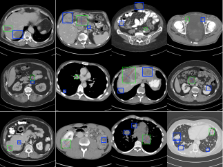
Figure 3: An illustration of the mined suspicious lesions on the DeepLesion training set. The original RECISTs produced annotations are represented by the green bounding boxes. The mined lesions with output confidence greater than 0.9 are indicated by the blue bounding boxes.

III Experiments

III-A Dataset and Metrics

DeepLesion [17] is the largest CT dataset for universal lesion detection at the moment, but it contains roughly 50% unlabeled lesions [2]. The original test set also has the missing annotation issue and could cause unreliable evaluation results. Cai et al. [10] fully annotated and released 1915 of the DeepLesion subvolumes. 844 subvolumes of them are selected from the original training set, in which 744 subvolumes are used for additional training, 100 subvolumes for validation. The other 1,071 subvolumes are used for the test. We also adopt this setting. Specifically, we use the same 100 fully annotated subvolumes to validate our model, the rest of the original training set to train our model. The 1071 fully annotated subvolumes are used for evaluation.

Similarly to previous studies, we report the average precision (AP) and the detection sensitivities at different false positive (FP) rates (0.125 to 8) per volume using the P3D IoU evaluation metric [10].

TABLE I: Average precision (AP) and sensitivity at various FPs per image on the fully annotated testing set of DeepLesion, the official annotated lesions, mined suspicious lesions by different methods and mined hard negative samples are denote as R, P+ and P- respectively.

Method				Sensitivity (%) at different FPs per subvolume
	R	P+	P-	0.125	0.25	0.5	1	2	4	8	AVG	AP (%)
Mask R-CNN [18]	✓			13.64	19.92	27.48	36.73	47.01	57.41	66.38	38.36	41.4
Yan et al. [7]	✓			11.43	18.69	26.98	38.99	50.15	60.38	69.71	39.47	41.8
Cai et al. [10]	✓			11.92	18.42	27.54	38.91	50.15	60.76	69.82	39.64	43.0
Lyu et al. [12]	✓			14.84	20.08	27.93	37.14	47.59	57.65	66.47	38.81	42.1
Ours	✓			18.63	25.45	32.78	40.43	49.00	57.51	65.67	41.32	45.0
Wang et al. [9]	✓	✓		15.88	20.98	29.41	38.36	47.89	58.14	67.89	39.79	43.2
Cai et al. [10]	✓	✓		13.41	19.16	27.34	37.54	49.33	60.52	70.18	39.64	43.6
Lyu et al. [12]	✓	✓		20.01	25.65	33.44	42.81	52.39	60.69	68.79	43.39	47.5
Ours	✓	✓		21.17	28.13	36.10	45.73	54.98	63.47	70.67	45.75	50.2
Cai et al. [10]	✓	✓	✓	19.86	27.11	36.21	46.82	56.89	66.82	74.73	46.92	51.9
Lyu et al. [12]	✓	✓	✓	30.89	37.28	43.94	51.05	57.41	63.68	69.81	50.58	54.7
Ours	✓	✓	✓	27.63	35.87	42.37	51.68	58.93	66.87	74.65	51.14	55.3

III-B Implementation Details

Our model is built on Faster R-CNN [16] using MMDetection toolbox [19]. We employ the ImageNet pretrained truncated DenseNet-121 [20] as the backbone, and each input contains 9 contiguous CT slices, as in earlier work [10, 12]. the CT slices are interpolated to 2 mm in the z-axis and 0.8 mm in the xy-plane. We rescale the 12-bit CT intensity range to [0,255] using a single windowing (-1024–3071 HU). We use random resize as the data augmentation method and the resize ratio for student model is [0.8,1.2]. The IoU threshold for GT NMS operation is 0.7 and the confidence filter threshold for mined lesion is set to $\tau=0.9$. The momentum value for EMA update is set to 0.999. We adopt stochastic gradient descent (SGD) optimizer to train the model for 80000 iterations with the learning rate $lr=0.02$. We do not use any learning rate decay schedule. The final model is chosen based on the performance on the validation set. It takes about 8 hours to train our model for 80000 iterations on 4 RTX-2080Ti GPUs.

III-C Main Results

Table I compares the performance of the proposed method and earlier state-of-the-art ULD methods on the fully annotated DeepLesion test set. MULAN [7] is one of the best-performing methods on the original partially labeled test set. Wang et al. [9], Cai et al. [10], and Lyn et al. [12] are three recent methods considered to mined the unlabeled lesions. In Lyn et al.’s [12] paper, the performance of the Mask-RCNN method is also reported. We also list it in the table. We first show the results trained only using the original annotations. As we can see, the EMA ensembled teacher branch achieves the overall best performance. In particular, it outperforms the second best model by 1.67% of the average sensitivity and 2.0% average precision, which demonstrates the useful ensemble effect of the EMA update policy.

For the lesion mining results, our method surpasses all other methods by a large margin. specifically, it outperforms the current state-of-the-art method [12] by 2.3% of the average sensitivity and 2.7% average precision, proving that our end-to-end method has better lesion mining capacity. We show some lesion mining results in Fig. 3. The green bounding boxes represent the original annotations. The mined lesions are shown in blue. In total, we mined about 8000 suspicious lesions on the DeepLesion training set.

Finally, for the completeness of comparative experiments, same to the method used in [12], we also apply our trained detector on the fully annotated training subvolumes and select the hard negative samples for retraining. Compared with [12], our method can find more lesions and show the best overall metric results.

III-D Ablation Studies

We start by verifying that the confidence filter’s threshold value is appropriate. We have done this by training our model for a total of 20000 iterations with various threshold settings. Table II displays the result. We report the average value of the sensitivitity at different FPs (AS) and average precision (AP). When the threshold is set to 0.9, the best results are obtained. In general, the higher the threshold, the more true positives it will reject, whereas the lower the threshold, the more false positives it will produce. When the threshold value is set to 0.80, the performance rapidly degrades due to the addition of too many false positive samples for training the student branch.

Next, we tested different strategies for using the mined lesions. The mined lesions are ignored by the previous approach [12]. We tested this strategy and set the ignore range as $[0.9,1)$ corresponding to the confidence filter’s threshold. The results are shown in Table III. Both of these strategies bring substantial performance gain and adding the mined lesions to ground truth can give best results.

TABLE II: Ablation study on different confidence filter threshold.

$\tau$ value	AS (%)	AP (%)
0.95	42.93	46.90
0.90	43.72	47.91
0.85	41.49	45.04
0.80	30.99	31.25

TABLE III: Comparison of different strategies for using the mined lesions.

Strategy	AS (%)	AP (%)
Adding	45.75	50.21
Ignoring	43.63	48.96

TABLE IV: Ablation study on the learning rate schedule.

LR Schedule	AS (%)	AP (%)
with LR decay	42.21	46.10
w/o LR decay	44.10	48.57

Learning rate decay is a commonly used technique for training neural networks. However, using the learning rate decay will harm the teacher’s performance in our scenario since our model mimics the ensemble model’s behavior. To demonstrate this, we first trained our model for 20000 iterations. On top of that, we trained another 20000 iterations with or without using learning rate decay. Table IV displays the results. It is clear that the model trained without learning rate decay outperforms the other.

IV Conclusion

In this paper, we present a novel end-to-end approach to dealing with missing annotations in the universal lesion detection task. We employ the teacher-student framework to mine unlabeled lesions and train the detector concurrently. Specifically, in each iteration, the teacher model infers the input data and creates a set of predictions. The high-confidence predictions are considered suspicious lesions and combined with partially-labeled ground truth to train the student model on the fly. The teacher model maintains an exponential moving average (EMA) of the student model and is used as the final output model. We tested two policies for dealing with the mined suspicious regions: ignoring them or adding them as mined pseudo ground truth. We discovered that learning rate decay would degrade the teacher’s performance and should not be employed. Instead, using a fixed learning rate can give us promising results. We evaluated our model against the state-of-the-art methods on the DeepLesion dataset. By using the original partially labeled training set, our model can outperform the previous best method by 2.3% on average sensitivity and 2.7% on average precision. Our method can also be used in other lesion detection problems where complete annotations is hard to acquire.

References

- [1] Y.-B. Tang, K. Yan, Y.-X. Tang, J. Liu, J. Xiao, and R. M. Summers, “Uldor: a universal lesion detector for ct scans with pseudo masks and hard negative example mining,” in 2019 IEEE 16th International Symposium on Biomedical Imaging (ISBI 2019). IEEE, 2019, pp. 833–836.
- [2] K. Yan, M. Bagheri, and R. M. Summers, “3d context enhanced region-based convolutional neural network for end-to-end lesion detection,” in International Conference on Medical Image Computing and Computer-Assisted Intervention. Springer, 2018, pp. 511–519.
- [3] U. Baid, S. Ghodasara, S. Mohan, M. Bilello et al., “The rsna-asnr-miccai brats 2021 benchmark on brain tumor segmentation and radiogenomic classification,” arXiv:2107.02314, 2021.
- [4] E. A. Eisenhauer, P. Therasse, J. Bogaerts, L. H. Schwartz, D. Sargent, R. Ford, J. Dancey, S. Arbuck, S. Gwyther, M. Mooney et al., “New response evaluation criteria in solid tumours: revised recist guideline (version 1.1),” European journal of cancer, vol. 45, no. 2, pp. 228–247, 2009.
- [5] Z. Li, S. Zhang, J. Zhang, K. Huang, Y. Wang, and Y. Yu, “Mvp-net: multi-view fpn with position-aware attention for deep universal lesion detection,” in International Conference on Medical Image Computing and Computer-Assisted Intervention. Springer, 2019, pp. 13–21.
- [6] Q. Tao, Z. Ge, J. Cai, J. Yin, and S. See, “Improving deep lesion detection using 3d contextual and spatial attention,” in International Conference on Medical Image Computing and Computer-Assisted Intervention. Springer, 2019, pp. 185–193.
- [7] K. Yan, Y. Tang, Y. Peng, V. Sandfort, M. Bagheri, Z. Lu, and R. M. Summers, “Mulan: Multitask universal lesion analysis network for joint lesion detection, tagging, and segmentation,” in MICCAI. Springer, 2019, pp. 194–202.
- [8] S. Zhang, J. Xu, Y.-C. Chen, J. Ma, Z. Li, Y. Wang, and Y. Yu, “Revisiting 3d context modeling with supervised pre-training for universal lesion detection in ct slices,” in International Conference on Medical Image Computing and Computer-Assisted Intervention. Springer, 2020, pp. 542–551.
- [9] Z. Wang, Z. Li, S. Zhang, J. Zhang, and K. Huang, “Semi-supervised lesion detection with reliable label propagation and missing label mining,” in Chinese Conference on Pattern Recognition and Computer Vision (PRCV). Springer, 2019, pp. 291–302.
- [10] J. Cai, A. P. Harrison, Y. Zheng, K. Yan, Y. Huo, J. Xiao, L. Yang, and L. Lu, “Lesion-harvester: Iteratively mining unlabeled lesions and hard-negative examples at scale,” IEEE Transactions on Medical Imaging, vol. 40, no. 1, pp. 59–70, 2020.
- [11] K. Yan, J. Cai, Y. Zheng, A. P. Harrison, D. Jin, Y.-b. Tang, Y.-X. Tang, L. Huang, J. Xiao, and L. Lu, “Learning from multiple datasets with heterogeneous and partial labels for universal lesion detection in ct,” IEEE Transactions on Medical Imaging, 2020.
- [12] F. Lyu, B. Yang, A. J. Ma, and P. C. Yuen, “A segmentation-assisted model for universal lesion detection with partial labels,” in MICCAI. Springer, 2021, pp. 117–127.
- [13] A. Shrivastava, A. Gupta, and R. Girshick, “Training region-based object detectors with online hard example mining,” in Proceedings of the IEEE conference on computer vision and pattern recognition, 2016, pp. 761–769.
- [14] Z. Wu, N. Bodla, B. Singh, M. Najibi, R. Chellappa, and L. S. Davis, “Soft sampling for robust object detection,” arXiv preprint arXiv:1806.06986, 2018.
- [15] A. Tarvainen and H. Valpola, “Mean teachers are better role models: Weight-averaged consistency targets improve semi-supervised deep learning results,” arXiv:1703.01780, 2017.
- [16] S. Ren, K. He, R. Girshick, and J. Sun, “Faster r-cnn: Towards real-time object detection with region proposal networks,” Advances in neural information processing systems, vol. 28, 2015.
- [17] K. Yan, X. Wang, L. Lu, and R. M. Summers, “Deeplesion: automated mining of large-scale lesion annotations and universal lesion detection with deep learning,” Journal of medical imaging, vol. 5, no. 3, p. 036501, 2018.
- [18] K. He, G. Gkioxari, P. Dollár, and R. Girshick, “Mask r-cnn,” in Proceedings of the IEEE international conference on computer vision, 2017, pp. 2961–2969.
- [19] K. Chen, J. Wang, J. Pang, Y. Cao, Y. Xiong, X. Li, S. Sun, W. Feng, Z. Liu, J. Xu, Z. Zhang, D. Cheng, C. Zhu, T. Cheng, Q. Zhao, B. Li, X. Lu, R. Zhu, Y. Wu, J. Dai, J. Wang, J. Shi, W. Ouyang, C. C. Loy, and D. Lin, “MMDetection: Open mmlab detection toolbox and benchmark,” arXiv preprint arXiv:1906.07155, 2019.
- [20] G. Huang, Z. Liu, L. Van Der Maaten, and K. Q. Weinberger, “Densely connected convolutional networks,” in Proceedings of the IEEE conference on computer vision and pattern recognition, 2017, pp. 4700–4708.