Algorithms for square root of semi-infinite quasi-Toeplitz $M$-matrices

Abstract

A quasi-Toeplitz $M$-matrix $A$ is an infinite $M$-matrix that can be written as the sum of a semi-infinite Toeplitz matrix and a correction matrix. This paper is concerned with computing the square root of invertible quasi-Toeplitz $M$-matrices which preserves the quasi-Toeplitz structure. We show that the Toeplitz part of the square root can be easily computed through evaluation/interpolation at the $m$ roots of unity. This advantage allows to propose algorithms solely for the computation of correction part, whence we propose a fixed-point iteration and a structure-preserving doubling algorithm. Additionally, we show that the correction part can be approximated by solving a nonlinear matrix equation with coefficients of finite size followed by extending the solution to infinity. Numerical experiments showing the efficiency of the proposed algorithms are performed..

1 Introduction

$M$-matrices in the context of infinite dimensional spaces are called M-operators, which, to our knowledge, were firstly investigated in [19], since then related theoretical properties have been developed in [1, 18, 19, 20, 21, 25]. Quasi-Toeplitz $M$-matrices are infinite $M$-matrices with an almost Toeplitz structure, they are encountered in the numerical solution of a quadratic matrix equation [11] involved in 2-dimensional Quasi-Birth-Death (QBD) stochastic processes [23] and are recently studied in [16] in terms of their theoretical and computational properties.

In this paper, we are interested in the quasi-Toeplitz $M$-matrices that belongs to the class $\mathcal{QT}_{\infty}=\{T(a)+E:a(z)\in\mathcal{W},E\in\mathcal{K}_{d}(\ell^{\infty})\}$, where $T(a)$ is a semi-infinite Toeplitz matrix associated with the function $a(z)=\sum_{i\in\mathbb{Z}}a_{i}z^{i}$ in the sense that $(T(a))_{i,j}=a_{j-i}$, $\mathcal{W}$ is the Wiener algebra, defined as the set $\mathcal{W}=\{a(z)=\sum_{i\in\mathbb{Z}}a_{i}z^{i}:z\in\mathbb{T},\|a\|_{{}_{{}_{\mathcal{W}}}}:=\sum_{i\in\mathbb{Z}}|a_{i}|<\infty\}$, and $\mathcal{K}_{d}(\ell^{\infty})=\{E=(e_{i,j})_{i,j\in\mathbb{Z}^{+}}:\lim_{i}\sum_{j=1}^{\infty}|e_{i,j}|=0\}$. It has been proved in [9, Theorem 2.16] that the class $\mathcal{QT}_{\infty}$ is a Banach algebra with the infinity matrix norm $\|\cdot\|_{\infty}$, which turns out to be $\|A\|_{\infty}=\sup_{i}\sum_{j=1}^{\infty}|a_{i,j}|$ for $A=(a_{i,j})_{i,j\in\mathbb{Z}^{+}}$. For $A=T(a)+E\in\mathcal{Q}\mathcal{T}_{\infty}$, $T(a)$ is called the Toeplitz part with a symbol $a$, $E$ is called the correction part. Matrices in the class $\mathcal{Q}\mathcal{T}_{\infty}$ have rich and elegant theoretical and computational properties, we refer the reader to [3, 4, 5, 6, 7, 8, 9, 10, 11, 22, 24] for more details.

For a quasi-Toeplitz $M$-matrix $A=T(a)+E_{A}\in\mathcal{Q}\mathcal{T}_{\infty}$, it has been proved in [16] that if $A$ is an (invertible) $M$-matrix, then $T(a)$ is also an (invertible) $M$-matrix. Moreover, it shows that if $A$ is invertible, there exists a unique quasi-Toeplitz $M$-matrix $S=T(s)+E_{S}\in\mathcal{Q}\mathcal{T}_{\infty}$ such that $A=S^{2}$. Concerning the computation of matrix $S$, Binomial iteration and Cyclic Reduction (CR) algorithm have been proposed in [16], where the CR algorithm seems to be better suited in the numerical computations. However, both the Binomial iteration and the CR algorithm exploit the quasi-Toeplitz structure indirectly by performing approximate operations of semi-infinite quasi-Toeplitz matrices in the format. It would be natural to ask whether the quasi-Toeplitz structure can be fully exploited to propose more efficient algorithms.

Suppose $B=T(b)+E_{B}\in\mathcal{Q}\mathcal{T}_{\infty}$ satisfies $(I-B)^{2}=A$, where $A=T(a)+E_{A}$ is a given quasi-Toeplitz $M$-matrix, then we have for the symbols of the Toeplitz parts that $(1-b(z))^{2}=a(z)$. Observe that for a positive integer $n>0$, there is always a unique Laurent polynomial $\hat{b}(z)=\sum_{i=-n+1}^{n}\hat{b}z^{i}$ that interpolates $b(z)$ at the $2n$ roots of unity. Based on the technic of evaluation/interpolation, we investigate computation of the coefficients $b_{i}$ of $b(z)=\sum_{i\in\mathbb{Z}}b_{i}z^{i}$, so that the Toeplitz part $T(b)$ of the quasi-Toeplitz $M$-matrix $A$ can be easily obtained.

Concerning the computation of the correction part, we propose a fixed-point iteration with a linear convergence rate, and a structure-preserving doubling algorithm, which is of quadratic convergence rate. Moreover, we show that the correction part can be approximated by extending a finite size matrix to infinity, where the finite size matrix solves a nonlinear matrix equation. Numerical experiments show that the proposed algorithms provide convergence acceleration in terms of CPU times comparing with the Binomial iteration and CR algorithm proposed in [16], both of which keep the whole quasi-Toeplitz matrices in the computations.

This paper is organized as follows. In the remaining part of this introduction, we recall some definitions and properties concerning quasi-Toeplitz matrices and $M$-matrices. Sections 2 and 3 concern with algorithms that fully exploit the quasi-Toeplitz structure of square root of invertible quasi-Toeplitz $M$-matrices, in Section 2 we show how the Toeplitz part is computed, while in Section 3, we design and analyze the convergence of algorithms that are applicable in computing the correction part. In Section 4, we show that the correction part can be approximated by extending to infinity of the solution of a nonlinear matrix equation with finite size coefficients. In Section 5, we show by numerical examples the efficiency of the proposed algorithms.

1.1 Preliminary concepts

Let $\ell^{\infty}$ be the space of sequences $\{x=(x_{1},x_{2},\ldots)\}$ such that $\sup_{i\in\mathbb{Z}^{+}}|x_{i}|<\infty$, one can see that quasi-Toeplitz $M$-matrices in the class $\mathcal{Q}\mathcal{T}_{\infty}$ are bounded linear operators from $\ell^{\infty}$ to $\ell^{\infty}$. Denote by $\mathcal{B}(\ell^{\infty})$ the Banach space of bounded linear operators from $\ell^{\infty}$ to itself, we first recall definition of $M$-operators on $\mathcal{B}(\ell^{\infty})$. For definition of more general $M$-operators on a real partially ordered Banach space, we refer the reader to [18, 21, 25] and the references therein. $M$-operators on the Banach space $\ell^{\infty}$ are defined as

Definition 1.1.

An operator $A\in\mathcal{B}(\ell^{\infty})$ is said to be a $Z$-operator if $A=sI-P$, with $s\geq 0$, $P(\ell^{\infty}_{+})\subseteq\ell^{\infty}_{+}$, where $\ell^{\infty}_{+}=\{x=(x_{i})_{i\in\mathbb{Z}^{+}}\in\ell^{\infty}:x_{i}\geq 0\ for\ all\ i\}$. A $Z$-operator is said to be an $M$-operator if $s\geq\rho(P)$, where $\rho(P)$ is the spectral radius of $P$. $A$ is an invertible $M$-operator if $s>\rho(P)$.

As matrices in $\mathcal{Q}\mathcal{T}_{\infty}$ can be represented as a matrix of infinite size, we keep using the term $M$-matrix when referring $M$-operators in $\mathcal{Q}\mathcal{T}_{\infty}$. This way, a matrix $A\in\mathcal{Q}\mathcal{T}_{\infty}$ is said to be an $M$-matrix if $A=\beta I-B$ with $B\geq 0$ and $\beta\geq\rho(B)$, and $A$ is invertible if $\beta>\rho(B)$. Here $B\geq 0$ means that $B$ is an elementwise nonnegative infinite matrix.

The following lemma contains a collection of properties of quasi-Toeplitz matrices and quasi-Toeplitz $M$-matrices, where properties (i) and (ii) have been proved in [13], while properties (iii) - (v) can be found from [16].

Lemma 1.2.

If $A=T(a)+E_{A}\in\mathcal{Q}\mathcal{T}_{\infty}$ and $B=T(b)+E_{B}\in\mathcal{Q}\mathcal{T}_{\infty}$, then the following properties hold:

• $AB=T(ab)-H(a^{-})H(a^{+})\in\mathcal{Q}\mathcal{T}_{\infty}$, where $(H(a^{-}))_{i,j}=(a_{-i-j+1})_{i,j\in\mathbb{Z}^{+}}$ and $(H(a^{+}))_{i,j}=(a_{i+j-1})_{i,j\in\mathbb{Z}^{+}}$;

• it holds that $\|a\|_{{}_{{}_{\mathcal{W}}}}=\|T(a)\|_{\infty}\leq\|A\|_{\infty}$;

• $T(a)\geq 0$ if $A\geq 0$.

• $\|a\|_{{}_{{}_{\mathcal{W}}}}=a(1)$ if $T(a)\geq 0$.

• T(a) is an (invertible) $M$-matrix if $A$ is an (invertible) $M$-matrix.

The following lemma shows that an invertible $M$-matrix in the class $\mathcal{Q}\mathcal{T}_{\infty}$ admits a unique quasi-Toeplitz $M$-matrix as a square root.

Lemma 1.3.

[16, Theorem 3.6] Suppose $A=\beta(I-A_{1})\in\mathcal{Q}\mathcal{T}_{\infty}$ satisfies $\beta>0$, $A_{1}\geq 0$ and $\|A_{1}\|_{\infty}<1$, then there is a unique $B\in\mathcal{Q}\mathcal{T}_{\infty}$ such that $B\geq 0,\|B\|_{\infty}<1$, and $(I-B)^{2}=I-A_{1}$.

For quasi-Toeplitz $M$-matrix $A=\gamma(I-A_{1})\in\mathcal{Q}\mathcal{T}_{\infty}$ such that $A_{1}\geq 0$ and $\|A_{1}\|_{\infty}<1$, it can be seen from Lemma 1.3 that it suffices to compute matrix $B$ such that $(I-B)^{2}=I-A_{1}$. In what follows, we propose algorithms for computing the Toeplitz part and the correction part of matrix $B$.

2 Computing the Toeplitz part

Observe that the Toeplitz part $T(b)$ is uniquely determinate by the coefficients $b_{j}$ of the symbol $b(z)=\sum_{j\in\mathbb{Z}}b_{j}z^{j}$. In this section, we show that $b(z)$ can be approximated by $\hat{b}(z)=\sum_{i=-n+1}^{n}\hat{b}_{j}z^{j}$ in the sense that $\|b-\hat{b}\|_{{}_{{}_{\mathcal{W}}}}\leq c\epsilon$ for some constant $c$ and a given tolerance $\epsilon$.

Suppose $B=T(b)+E_{B}$ satisfies $\gamma(I-B)^{2}=A$, where $A=\gamma(I-A_{1})\in\mathcal{Q}\mathcal{T}_{\infty}$ is such that $A_{1}\geq 0$ and $\|A_{1}\|_{\infty}<1$. Suppose $T(a)$ is the Toeplitz part of $A$, we have from property (i) of Lemma 1.2 that $\gamma(1-b(z))^{2}=a(z)$, that is,

$$a(z)/\gamma=b(z)^{2}-2b(z)+1,$$ (1)

from which we obtain $b(z)=1\pm\sqrt{a(z)/\gamma}$. Since $A_{1}\geq 0$, in view of properties (ii)-(iv) of Lemma 1.2, we have $a_{1}(1)=\|a_{1}\|_{{}_{{}_{\mathcal{W}}}}\leq\|A_{1}\|_{\infty}<1$, where $a_{1}(z)$ is the symbol of the Toeplitz part of $A_{1}$, hence we deduce that $a(1)=\gamma(1-a_{1}(1))>0$. On the other hand, it follows from $B\geq 0$ that $b(1)=\|b\|_{{}_{{}_{\mathcal{W}}}}=\|T(b)\|_{\infty}\leq\|B\|_{\infty}<1$, which, together with $\sqrt{a(1)/\gamma}>0$, implies that $b(1)=1-\sqrt{a(1)/\gamma}$ and therefore $b(z)=1-\sqrt{a(z)/\gamma}$.

Let $n>0$ be a positive integer, set $m=2n$, then there is always a unique Laurent series $\hat{b}(z)=\sum_{j=-n+1}^{n}\hat{b}_{j}z^{j}$ such that $\hat{b}(\omega_{m}^{\ell})=b(\omega_{m}^{\ell})$, $\ell=-n+1,\ldots,n$, where $\omega_{m}$ is the principal $m$-th root of 1, that is, $\omega_{m}=\cos\frac{2\pi}{m}+{\bf i}\sin\frac{2\pi}{m}$. Based on the evaluation/interpolation technique, where the interpolation can be done by the means of the Fast Fourier Transform (FFT), an approximation $\hat{b}_{i}$, $i=-n+1,...,n$, to the coefficients $b_{i}$ of $b(z)$ can be obtained. Since $B\geq 0$, we have from property (iii) of Lemma 1.2 that $T(b)\geq 0$, so that $b(z)=\sum_{i\in\mathbb{Z}}b_{i}z^{i}$ has nonnegative coefficients. If in addition $b^{\prime\prime}(z)\in\mathcal{W}$, the following lemma provides a bound to $|\hat{b}_{i}-b_{i}|$.

Lemma 2.1.

[11, Lemma 3.1] For $g=\sum_{i\in\mathbb{Z}}g_{i}z^{i}\in\mathcal{W}$ with nonnegative coefficients, let $\hat{g}(z)=\sum_{j=-n+1}^{n}\hat{g}_{j}z^{j}$ be the Laurent polynomial interpolating $g(z)$ at the $m$-th roots of 1, i.e., $g(w_{m}^{i})=\hat{g}(w_{m}^{i})$ for $i=-n+1,\ldots,n$, where $m=2n$. If $g^{\prime\prime}(t)\in\mathcal{W}$, then $g^{\prime\prime}(1)\geq 0$ and

$$g^{\prime\prime}(1)-\hat{g}^{\prime\prime}(1)\geq 2n\big{(}\sum_{j<-n+1}g_{j}+\sum_{j>n}g_{j}\big{)}.$$

Moreover, $0\leq\hat{g}_{j}-g_{j}\leq\frac{1}{2n}(g^{\prime\prime}(1)-\hat{g}^{\prime\prime}(1))$ for $j=-n+1,\ldots,n$.

For $\hat{b}(z)=\sum_{j=-n+1}^{n}\hat{b}_{j}z^{j}$ interpolating $b(z)$ at $\omega_{m}^{i}$ for $i=-n+1,\ldots,n$, suppose $b^{\prime\prime}(z)\in\mathcal{W}$ and $b^{\prime\prime}(1)>0$, we have from Lemma 2.1 that

$$b^{\prime\prime}(1)-\hat{b}^{\prime\prime}(1)\geq 2n\big{(}\sum_{j<-n+1}b_{j}+\sum_{j>n}b_{j}\big{)},$$ (2)

and

$$|\hat{b}_{j}-b_{j}|\leq\frac{1}{2n}(b^{\prime\prime}(1)-\hat{b}^{\prime\prime}(1)),\ j=-n+1,\ldots,n.$$ (3)

If $b^{\prime\prime}(1)-\hat{b}^{\prime\prime}(1)<\epsilon$ for a given tolerance $\epsilon>0$, we have from (3) that $|b_{j}-\hat{b}_{j}|\leq\epsilon/(2n)$ for $j=-n+1,\ldots,n$, which together with (2) implies that

$$\|b-\hat{b}\|_{{}_{{}_{\mathcal{W}}}} =\sum_{j=-n+1}^{n}|b_{j}-\hat{b}_{j}|+\sum_{j<-n+1}b_{j}+\sum_{j>n}b_{j}$$

$$\leq\epsilon+\frac{1}{2n}(b^{\prime\prime}(1)-\hat{b}^{\prime\prime}(1))$$

$$\leq(1+\frac{1}{2n})\epsilon.$$

Hence, in the computation of $\hat{b}_{j},j=-n+1,\ldots,n$, under the evaluation/interpolation scheme, the approximation is accurate enough if $b^{\prime\prime}(1)-\hat{b}^{\prime\prime}(1)<\epsilon$. Actually, the values of $b^{\prime\prime}(1)-\hat{b}^{\prime\prime}(1)$ can be easily obtained. Indeed, once the coefficients $\hat{b}_{j}$ of $\hat{b}(z)=\sum_{j=-n+1}^{n}\hat{b}_{j}z^{j}$ are computed, one can easily obtain $\hat{b}^{\prime\prime}(1)=\sum_{j=-n+1}^{n}j(j-1)\hat{b}_{j}$. On the other hand, we have from equation (1) that

$$b^{\prime}(z)=\frac{a^{\prime}(z)}{2\gamma(b(z)-1)}\ {\rm and}\ b^{\prime\prime}(z)=\frac{a^{\prime\prime}(z)-2\gamma(b^{\prime}(z))^{2}}{2\gamma(b(z)-1)},$$

from which we easily obtain $b^{\prime}(1)$ and $b^{\prime\prime}(1)$.

Observe that equation (1) is a special case of the quadratic equation

$$a_{1}(z)g(z)^{2}+(a_{0}(z)-1)g(z)+a_{-1}(z)=0,$$

where $a_{i}(z)$ for $i=-1,0,1$ are known functions in the class $\mathcal{W}$ and $g(z)$ is the function to be determined. Algorithms for computing the approximations of the coefficients of $g(z)$ has been proposed in [11], based on which we propose the following Algorithm 1 that is more efficient in computing the coefficients $\hat{b}_{j}$ of the Laurent series $\hat{b}(z)=\sum_{j=-n+1}^{n}\hat{b}_{j}z^{j}$, so that we get an approximation $T(\hat{b})$ to the Toeplitz part $T(b)$ in the sense that $\|T(b)-T(\hat{b})\|_{\infty}=\|b-\hat{b}\|_{{}_{{}_{\mathcal{W}}}}\leq(1+\frac{1}{2n})\epsilon$ for a given tolerance $\epsilon$.

Algorithm 1 Approximation of $b(z)$

0:  The coefficients of $a(z)$, a scalar $\gamma$ such that $A=\gamma(I-A_{1})$ and a tolerance $\epsilon>0$.

0:  Approximations $\hat{b}_{j}$, $j=-n+1,\ldots,n$, to the coefficients $b_{j}$ of $b(z)$ such that $|\hat{b}_{j}-b_{j}|\leq\epsilon/(2n)$.

1:  Set n=4, and compute $b(1)=1-\sqrt{a(1)/\gamma}$ and $b^{\prime}(1)=\frac{a^{\prime}(1)}{2\gamma(b(1)-1)}$ and $b^{\prime\prime}(1)=\frac{a^{\prime\prime}(1)-2\gamma(b^{\prime}(1))^{2}}{2\gamma(b(1)-1)}$;

2:  Set $m=2n$ and $w_{m}=\cos\frac{2\pi}{m}+{\bf i}\sin\frac{2\pi}{m}$. Evaluate $a(z)$ at $z=w_{m}^{i}$ for $i=-n+1,\ldots,n$;

3:  For $i=-n+1,\ldots,n$, compute $s_{i}=1-\sqrt{a(\omega_{m}^{i})/\gamma}$;

4:  Interpolate the values $s_{i}$, $i=-n+1,\ldots,n$, by means of FFT and obtain the coefficients $\hat{b}_{j}$ of the Laurent polynomial $\hat{b}(z)=\sum_{j=-n+1}^{n}\hat{b}_{j}z^{j}$ such that $b(w_{m}^{i})=\hat{b}(w_{m}^{i})$, $i=-n+1,\ldots,n$;

5:  Compute $\hat{b}^{\prime\prime}(1)=\sum_{j=-n+1}^{n}j(j-1)\hat{b}_{j}$ and $\delta_{m}=b^{\prime\prime}(1)-\hat{b}^{\prime\prime}(1)$;

6:  If $\delta_{m}<\epsilon$ then exit, else set $n=2n$ and compute from Step 2.

It can be seen that the overall computational cost of Algorithm 1 is $O(n\log n)$ arithmetic operations. Now the Toeplitz part of matrix $B$ is approximated by $T(\hat{b})$, it remains to compute the correction part of $B$ in order to complete the computation of the square root. We show this subject in next section.

3 Computing the correction part

Suppose $A=\beta(I-A_{1})\in\mathcal{Q}\mathcal{T}_{\infty}$, where $A_{1}\geq 0$ and $\|A_{1}\|_{\infty}<1$, then for $B=T(b)+E_{B}\geq 0$ and $\|B\|_{\infty}<1$ such that $(I-B)^{2}=I-A_{1}$, we design and analyze the convergence of a fixed-point iteration and a structure-preserving doubling algorithm that can be used for the computation of $E_{B}$.

3.1 Fixed-point iteration

Consider the nonlinear matrix equation

$$(I-T(b)-X)^{2}=I-A_{1}$$

which can be equivalently written as

$$X^{2}-(I-T(b))X-X(I-T(b))+Q=0,$$ (4)

where $Q=A_{1}+T(b)^{2}-2T(b)$. It is clear that $E_{B}$ solves equation (4). On the other hand, it follows from Lemma 1.3 that $I-A_{1}$ allows a unique quasi-Toeplitz $M$-matrix as a square root, so that $E_{B}$ is the unique solution of equation (4) such that $T(b)+E_{B}\geq 0$ and $\|T(b)+E_{B}\|_{\infty}<1$.

Observe that equation (4) can be equivalently written as $X=(2I-T(b)-X)^{-1}(Q+XT(b))$, from which we propose the following iteration

$$X_{k+1}=(2I-T(b)-X_{k})^{-1}(Q+X_{k}T(b))$$ (5)

with $X_{0}=0$. We show that the sequence $\{X_{k}\}$ converges to $E_{B}$. To this end, we first show the following result.

Theorem 3.1.

Let $A=\beta(I-A_{1})\in\mathcal{QT}_{\infty}$ with $A_{1}\geq 0$ and $\|A_{1}\|_{\infty}<1$. Suppose $B=T(b)+E_{B}\in\mathcal{Q}\mathcal{T}_{\infty}$ is the unique quasi-Toeplitz matrix such that $B\geq 0$, $\|B\|_{\infty}<1$, and $(I-B)^{2}=I-A_{1}$. Then, the sequence $\{X_{k}\}$ generated by iteration (5) satisfies

• the sequence $\{X_{k}\}$ is well defined;

• $T(b)+X_{k}\geq 0$ and $\|T(b)+X_{k}\|_{\infty}<1$.

Proof.

Concerning item (i), observe that $X_{k+1}$ is well defined as long as $2I-T(b)-X_{k}$ is invertible. It follows from [17, Lemma 3.1.5] that $2I-T(b)-X_{k}$ is invertible if $\|T(b)+X_{k}\|_{\infty}<2$, which can be verified if item (ii) is true. Hence, it suffices to prove item (ii).

We prove item (ii) by induction. For $k=0$, we have $T(b)+X_{0}=T(b)\geq 0$, where the inequality follows from property (iii) of Lemma 1.2 and the fact $B\geq 0$. On the other hand, we have from property (ii) of Lemma 1.2 that $\|T(b)+X_{0}\|_{\infty}\leq\|B\|_{\infty}<1$. For the inductive step, assume that $T(b)+X_{k}\geq 0$ and $\|T(b)+X_{k}\|_{\infty}<1$, we show that $T(b)+X_{k+1}\geq 0$ and $\|T(b)+X_{k+1}\|_{\infty}<1$.

Observe that

$$X_{k+1} =(2I-T(b)-X_{k})^{-1}(A_{1}-(2I-T(b)-X_{k})T(b))$$

$$=(2I-T(b)-X_{k})^{-1}A_{1}-T(b),$$

from which we have

$$T(b)+X_{k+1}=(2I-T(b)-X_{k})^{-1}A_{1}.$$

It follows from [17, Lemma 3.1.5] that

$$(2I-T(b)-X_{k})^{-1}=\frac{1}{2}\sum_{i=0}^{\infty}\big{(}\frac{1}{2}(T(b)+X_{k})\big{)}^{i},$$

so that $(2I-T(b)-X_{k})^{-1}\geq 0$ since $T(b)+X_{k}\geq 0$. Recall that $A_{1}\geq 0$, we thus have $(2I-T(b)-X_{k})^{-1}A_{1}\geq 0$, that is, $T(b)+X_{k+1}\geq 0$.

It remains to show $\|T(b)+X_{k+1}\|_{\infty}<1$. Observe that

$$\|T(b)+X_{k+1}\|_{\infty} =\|(2I-T(b)-X_{k})^{-1}A_{1}\|_{\infty}$$

$$\leq\|(2I-T(b)-X_{k})^{-1}\|_{\infty}\|A_{1}\|_{\infty}$$

$$\leq\frac{\|A_{1}\|_{\infty}}{2-\|T(b)+X_{k}\|_{\infty}},$$

where the last inequality holds since

$$\|(2I-T(b)-X_{k})^{-1}\|_{\infty} \leq\frac{1}{2}\sum_{i=0}^{\infty}\big{(}\frac{1}{2}\|T(b)+X_{k}\|_{\infty}\big{)}^{i}$$

$$=\frac{1}{2-\|T(b)+X_{k}\|_{\infty}}.$$ (6)

Recall that $\|T(b)+X_{k}\|_{\infty}<1$ and $\|A_{1}\|_{\infty}<1$, one can check that

$$\frac{\|A_{1}\|_{\infty}}{2-\|T(b)+X_{k}\|_{\infty}}<1,$$

that is, $\|T(b)+X_{k+1}\|_{\infty}<1$. ∎

The following result shows the convergence of sequence $\{X_{k}\}$.

Theorem 3.2.

Let $A=\beta(I-A_{1})\in\mathcal{QT}_{\infty}$ with $A_{1}\geq 0$ and $\|A_{1}\|_{\infty}<1$. Suppose $B=T(b)+E_{B}\in\mathcal{Q}\mathcal{T}_{\infty}$ is the unique quasi-Toeplitz matrix such that $B\geq 0$, $\|B\|_{\infty}<1$ and $(I-B)^{2}=I-A_{1}$. Then the sequence $\{X_{k}\}$ generated by iteration (5) converges to $E_{B}$ in the sense that $\lim_{k\rightarrow\infty}\|E_{B}-X_{k}\|_{\infty}=0$.

Proof.

Let $E_{k}=E_{B}-X_{k}$, a direct computation yields

$$E_{k+1}=(2I-T(b)-X_{k})^{-1}E_{k}B,$$

which, together with (3.1), yields

$$\|E_{k+1}\|_{\infty}\leq\frac{\|B\|_{\infty}}{2-\|T(b)+X_{k}\|_{\infty}}\|E_{k}\|_{\infty}.$$ (7)

Since $\|T(b)+X_{k}\|_{\infty}<1$, it follows that $\frac{\|B\|_{\infty}}{2-\|T(b)+X_{k}\|_{\infty}}<\|B\|_{\infty}$, so that

$$\|E_{k+1}\|_{\infty}\leq\|B\|_{\infty}\|E_{k}\|_{\infty}\leq\|B\|_{\infty}^{k}\|E_{0}\|_{\infty}.$$

Since $\|B\|_{\infty}<1$, it implies that $\lim_{k\rightarrow\infty}\|E_{B}-X_{k}\|_{\infty}=0$. ∎

We may observe from inequality (7) that the sequence $\{X_{k}\}$ generated by iteration (5) satisfies $\|X_{k+1}-E_{B}\|_{\infty}\leq\frac{\|B\|_{\infty}}{2-\|T(b)+X_{k}\|_{\infty}}\|X_{k}-E_{B}\|_{\infty}$. The fact $\frac{\|B\|_{\infty}}{2-\|T(b)+X_{k}\|_{\infty}}<\|B\|_{\infty}$ may provide some insights to say that the fixed-point iteration (5), which is used for the computation of the correction part, converges faster than the Binomial iteration [16] in the computation of the whole square root, as the sequence $\{Y_{k}\}$ generated by the Binomial iteration $Y_{k+1}=\frac{1}{2}(A_{1}+Y_{k}^{2})$ with $Y_{0}=0$ satisfies that $\|Y_{k+1}-B\|_{\infty}\leq\|B\|_{\infty}\|Y_{k}-B\|_{\infty}$.

3.2 Structure-preserving Doubling Algorithm

We show that a structure-preserving doubling algorithm (SDA) is applicable in the computation of $E_{B}$ such that $(I-T(b)-E_{B})^{2}=A$, where $A$ is an invertible quasi-Toeplitz $M$-matrix. This method has been motivated by the ideas in [12], where the SDA that enables refining an initial approximation is applied to solve quadratic matrix equations with quasi-Toeplitz coefficients. We fist recall the design and convergence analysis of SDA. For more details of SDA, we refer the reader to [12], [2, Chapter 5] and [15].

In the finite dimensional space, the design of SDA is based on a linear pencil $M-\lambda N$, where $M$ and $N$ are $2n\times 2n$ matrices of the form

$$M=\left[\begin{array}[]{cc}E&O\\ -P&I\end{array}\right],\quad N=\left[\begin{array}[]{cc}I&-Q\\ O&F\end{array}\right],$$ (8)

where $E,F,P,Q$ are $n\times n$ matrices, $I$ and $O$ are, respectively, the $n\times n$ identity matrix and the zero matrix. Suppose there are $n\times n$ matrices $X$ and $W$ such that

$$M\left[\begin{array}[]{c}I\\ X\end{array}\right]=N\left[\begin{array}[]{c}I\\ X\end{array}\right]W.$$

Then, the SDA consists in computing the sequences defined as

$$E_{k+1} =E_{k}(I-Q_{k}P_{k})^{-1}E_{k}$$ (9)

$$P_{k+1} =P_{k}+F_{k}(I-P_{k}Q_{k})^{-1}P_{k}E_{k};$$

$$F_{k+1} =F_{k}(I-P_{k}Q_{k})^{-1}F_{k};$$

$$Q_{k+1} =Q_{k}+E_{k}(I-Q_{k}P_{k})^{-1}Q_{k}F_{k},$$

where $E_{0}=E,F_{0}=F,P_{0}=P$ and $Q_{0}=Q$.

We mention that the scheme (9) is quite related to the forms of matrices $M$ and $N$ in (8), which is called the standard structured form-I. For different forms, say the standard structured form-II (see [2, Chapter 5]), different schemes can be obtained.

Concerning the convergence results of SDA, it has been proved in [12] that

Lemma 3.3.

[12, Theorem 2] Let $X,Y,W,V$ be $n\times n$ matrices such that

$$M\left[\begin{array}[]{c}I\\ X\end{array}\right]=N\left[\begin{array}[]{c}I\\ X\end{array}\right]W,\quad M\left[\begin{array}[]{c}Y\\ I\end{array}\right]V=N\left[\begin{array}[]{c}Y\\ I\end{array}\right],$$

and it satisfies that $\rho(W)\leq 1$, $\rho(V)\leq 1$, $\rho(W)\rho(V)<1$. If the scheme (9) can be carried out with no breakdown, then $\lim_{k}\|X-P_{k}\|^{1/{2^{k}}}\leq\rho(W)\rho(V)$ and $\lim_{k}\|Y-Q_{k}\|^{1/{2^{k}}}\leq\rho(W)\rho(V)$.

Concerning the feasibility of SDA in the infinite dimensional spaces, it has been shown in [12, page 11] that the convergence results of SDA still hold when matrices belonging to the Banach algebra $\mathcal{Q}\mathcal{T}_{\infty}$. We are ready to show how SDA can be applied in the computation of $E_{B}$.

Suppose $A=I-A_{1}\in\mathcal{Q}\mathcal{T}_{\infty}$ is such that $A_{1}\geq 0$ and $\|A_{1}\|_{\infty}<1$, we have from Lemma 1.3 that the matrix equation

$$(I-X)^{2}=I-A_{1}$$ (10)

has a unique nonnegative solution $B\in\mathcal{Q}\mathcal{T}_{\infty}$ satisfying $\|B\|_{\infty}<1$. Observe that equation (10) can be equivalently written as

$$X^{2}-2X+A_{1}=0,$$ (11)

so that $B$ solves equation (11) and is the unique solution such that $B\geq 0$ and $\|B\|_{\infty}<1$. Let $V=(2I-B)^{-1}$, it is easy to check that $V$ solves the quadratic matrix equation

$$A_{1}Y^{2}-2Y+I=0.$$ (12)

Moreover, we have $V=\frac{1}{2}\sum_{i=0}^{\infty}(\frac{1}{2}B)^{i}\geq 0$ and $\|V\|_{\infty}\leq\frac{1}{2}\sum_{i=1}^{\infty}(\frac{1}{2}\|B\|_{\infty})^{i}=\frac{1}{2-\|B\|_{\infty}}<1$.

Suppose $T(b)$ with $b\in\mathcal{W}$ is the Toeplitz part of $B$, replacing $X$ by $T(b)+H$ in equation (11) results in the following quadratic matrix equation

$$H^{2}+(T(b)-2I)H+HT(b)+R=0,$$ (13)

where $R=T(b)^{2}-2T(b)+A_{1}$. Then, equation (13) can be equivalently written as

$$\widetilde{M}\left[\begin{array}[]{cc}I\\ H\end{array}\right]=\widetilde{N}\left[\begin{array}[]{cc}I\\ H\end{array}\right]B,$$

where $\widetilde{M}=\left[\begin{array}[]{cc}T(b)&I\\ -R&2I-T(b)\end{array}\right]$ and $\widetilde{N}=\left[\begin{array}[]{cc}I&0\\ 0&I\end{array}\right]$.

According to [12, Theorem 3], the pencil $\widetilde{M}-\lambda\widetilde{N}$ can be transformed into the pencil $\mathcal{M}-\lambda\mathcal{N}$, where $\mathcal{M}$ and $\mathcal{N}$ are of the form

$$\mathcal{M}=\left[\begin{array}[]{cc}SA_{1}&0\\ -SR&I\end{array}\right],\quad\mathcal{N}=\left[\begin{array}[]{cc}I&-S\\ 0&S\end{array}\right],$$

where $S=2I-T(b)$. It can be seen that $\mathcal{M}$ and $\mathcal{N}$ are of the same forms as those in (8), and we have

$$\mathcal{M}\left[\begin{array}[]{c}I\\ H\end{array}\right]=\mathcal{N}\left[\begin{array}[]{c}I\\ H\end{array}\right]B,$$

so that SDA can be applied to the pencil $\mathcal{M}-\lambda\mathcal{N}$, which consists of computing the sequences as defined in the scheme (9) by setting

$$P_{0}=E_{0}=(2I-T(b))^{-1}B,\quad\quad Q_{0}=F_{0}=S.$$

On the other hand, it can be verified that the matrices $\mathcal{M}$ and $\mathcal{N}$ also satisfy

$$\mathcal{M}\left[\begin{array}[]{c}Y\\ I\end{array}\right]Z=\mathcal{N}\left[\begin{array}[]{c}Y\\ I\end{array}\right],$$ (14)

where $Y=V(I-T(b)V)^{-1},Z=(I-T(b)V)V(I-T(b)V)^{-1}$. It can be seen that $Z$ has the same spectrum as $V$ so that $\rho(Z)=\rho(V)\leq\|V\|_{\infty}<1$, we then have from the fact $\rho(B)\leq\|B\|_{\infty}<1$ that $\rho(B)\rho(Z)<1$. Hence, according to Lemma 3.3, we obtain the following convergence result of SDA when applying to the pencil $\mathcal{M}-\lambda\mathcal{N}$.

Theorem 3.4.

For $A=I-A_{1}\in\mathcal{Q}\mathcal{T}_{\infty}$ such that $A_{1}\geq 0$ and $\|A_{1}\|_{\infty}<1$, suppose $I-B$ with $B=T(b)+E_{B}\in\mathcal{Q}\mathcal{T}_{\infty}$ is the unique quasi-Toeplitz $M$-matrix such that $(I-B)^{2}=A$. If the scheme (9) can be carried out with no breakdown, then the sequence $\{P_{k}\}$ converges to $E_{B}$ and it satisfies $\lim_{k}\|E_{B}-P_{k}\|^{1/{2^{k}}}\leq\rho(B)\rho(Z)$, where $Z=(I-T(b)V)(2I-B)^{-1}(I-T(b)V)^{-1}$ and $V=(2I-B)^{-1}$.

Actually, according to the ideas in [12], the scheme (9) allows to refine a given initial approximation to $E_{B}$, that is, if $E_{B}=\tilde{E}_{B}+D$, where $\tilde{E}_{B}$ is given and it satisfies $\|T(b)+\tilde{E}_{B}\|_{\infty}<1$, then SDA can be used to compute $D$. Indeed, if $H$ in equation (13)is replaced by $\tilde{E}_{B}+D$, it yields

$$D^{2}+(T(b)+\tilde{E}_{B}-2I)D+D(T(b)+\tilde{E}_{B})+\tilde{R}=0,$$ (15)

where $\tilde{R}=(T(b)+\tilde{E}_{B})^{2}-2(T(b)+\tilde{E}_{B})+A_{1}$. Analogously to the analysis above, we obtain the matrix pencil $\widehat{\mathcal{M}}-\lambda\widehat{N}$ such that

$$\widehat{\mathcal{M}}=\left[\begin{array}[]{cc}\tilde{S}A_{1}&0\\ -\tilde{S}\tilde{R}&I\end{array}\right],\quad\widehat{\mathcal{N}}=\left[\begin{array}[]{cc}I&-\tilde{S}\\ 0&\tilde{S}\end{array}\right],$$

where $\tilde{S}=(2I-T(b)-\tilde{E}_{B})^{-1}$, and it holds

$$\widehat{\mathcal{M}}\left[\begin{array}[]{c}I\\ D\end{array}\right]=\widehat{\mathcal{N}}\left[\begin{array}[]{c}I\\ D\end{array}\right]B,\quad\widehat{\mathcal{M}}\left[\begin{array}[]{c}\tilde{Y}\\ I\end{array}\right]\tilde{Z}=\widehat{\mathcal{N}}\left[\begin{array}[]{c}\tilde{Y}\\ I\end{array}\right],$$

where $\tilde{Y}=V(I-(T(b)+\tilde{E}_{B})V)^{-1},\tilde{Z}=(I-(T(b)+\tilde{E}_{B})V)V(I-(T(b)+\tilde{E}_{B})V)^{-1}$.

Now apply SDA to the pencil $\widehat{M}-\lambda\widehat{N}$, we obtain the sequences defined as

$$\tilde{E}_{k+1} =\tilde{E}_{k}(I-\tilde{Q}_{k}\tilde{P}_{k})^{-1}\tilde{E}_{k}$$ (16)

$$\tilde{P}_{k+1} =\tilde{P}_{k}+\tilde{F}_{k}(I-\tilde{P}_{k}\tilde{Q}_{k})^{-1}\tilde{P}_{k}\tilde{E}_{k};$$

$$\tilde{F}_{k+1} =\tilde{F}_{k}(I-\tilde{P}_{k}\tilde{Q}_{k})^{-1}\tilde{F}_{k};$$

$$\tilde{Q}_{k+1} =\tilde{Q}_{k}+\tilde{E}_{k}(I-\tilde{Q}_{k}\tilde{P}_{k})^{-1}\tilde{Q}_{k}\tilde{F}_{k},$$

where $P_{0}=E_{0}=\tilde{S}A_{1}$ and $Q_{0}=F_{0}=\tilde{S}$.

Observe that $\rho(\tilde{Z})=\rho(V)<1$, then according to Lemma 3.3 it holds that $\lim_{k}\|\tilde{P}_{k}-D\|_{\infty}^{1/{2^{k}}}<\rho(B)\rho(V)<1$, that is, the sequence $\{\tilde{P}_{k}\}$ converges to $D$, so that $E_{B}=\tilde{E}_{B}+D$ is computed.

One alternative is to set $\tilde{E}_{B}=(b(1)-T(b){\bf 1})e_{1}^{T}$, where ${\bf 1}=(1,1,\ldots)^{T}$ and $e_{1}=(1,0,\ldots)^{T}$, then $T(b)+\tilde{E}_{B}$ is a nonnegative substochastic matrix such that $(T(b)+\tilde{E}_{B}){\bf 1}=b(1){\bf 1}$. Numerical experiments in Section 5 shows that there are cases where a reduction in CPU time occurs when setting $\tilde{E}_{B}=(b(1)-T(b){\bf 1})e_{1}^{T}$ and applying iteration (16) for computing $D$.

We mention that when applying the fixed-point iteration and SDA to compute the correction part of a quasi-Toeplitz $M$-matrix, the computations rely on the package CQT-Toolbox of [10] which implements the operations of semi-infinite quasi-Toeplitz matrices. In next section, we show that the the fixed-point iteration and SDA can be applied to a finite dimensional nonlinear matrix equation, whose solution after extending to infinity is a good approximation to $E_{B}$.

4 Truncation to a finite dimensional matrix equation

Recall that the correction part of a quasi-Toeplitz matrix $A=T(a)+E\in\mathcal{Q}\mathcal{T}_{\infty}$ satisfies $\lim_{i}\sum_{j=1}^{\infty}|e_{i,j}|=0$ for $E=(e_{i,j})_{i,j\in\mathbb{Z}^{+}}$. Denote by $E^{(k)}$ the infinite matrix that coincides with the leading principal $k\times k$ submatrix of $E$ and is zero elsewhere, it follows form [9, Lemma 2.9] that there is a matrix $E^{(k)}$ such that $\lim_{k\rightarrow\infty}\|E-E^{(k)}\|_{\infty}=0$.

For an invertible $M$-matrix $A=I-A_{1}\in\mathcal{Q}\mathcal{T}_{\infty}$, suppose $(I-T(b)-E_{B})^{2}=A$, then for $E_{B}$ and a given $\epsilon>0$, there is a sufficiently large $k$ such that

$$\|E_{B}^{(k)}-E_{B}\|_{\infty}<\epsilon.$$ (17)

If we partition $E_{B}$ into $E_{B}=\left(\begin{array}[]{cc}E_{11}&E_{12}\\ E_{21}&E_{22}\end{array}\right)$, where $E_{11}$ is the principal $k\times k$ submatrix of $E_{B}$, $E_{12}\in\mathbb{R}^{k\times\infty}$, $E_{21}\in\mathbb{R}^{\infty\times k}$ and $E_{22}\in\mathbb{R}^{\infty\times\infty}$, it follows from $\|E_{B}^{(k)}-E_{B}\|_{\infty}<\epsilon$ that $\|E_{12}\|_{\infty}<\epsilon,\|E_{21}\|_{\infty}<\epsilon$ and $\|E_{22}\|_{\infty}<\epsilon$.

Let $W=2T(b)-A_{1}-T(b)^{2}$, then $T(b)$ and $W$ can be partitioned into $T(b)=\left(\begin{array}[]{cc}T_{11}&T_{12}\\ T_{21}&T_{22}\end{array}\right)$ and $W=\left(\begin{array}[]{cc}W_{11}&W_{12}\\ W_{21}&W_{22}\end{array}\right)$, where $T_{11}$ and $W_{11}$ are, respectively, the principal $k\times k$ submatrices of $T(b)$ and $W$. Substituting $E_{B},T(b)$ and $W$ into the equation $(I-T(b)-E_{B})^{2}=I-A_{1}$, we get

$$E_{11}^{2}-(I_{k}-T_{11})E_{11}-E_{11}(I_{k}-T_{11})=W_{11}-E_{12}E_{21}-E_{12}T_{21}-T_{12}E_{21},$$ (18)

where $I_{k}$ is the identity matrix of size $k$.

Consider the matrix equation

$$G^{2}-(I_{k}-T_{11})G-G(I_{k}-T_{11})=W_{11},$$ (19)

which is equivalent to

$$(I_{k}-T_{11}-G)^{2}=I-A_{11}-T_{12}T_{21},$$ (20)

where $A_{11}$ is the principal $k\times k$ submatrix of $A_{1}$. Observe that $A_{11}\geq 0$ and $T_{12}T_{21}\geq 0$, if in addition $\rho(A_{11}+T_{12}T_{21})<1$, which can be verified if $\|A_{11}+T_{12}T_{21}\|_{\infty}<1$, then $I-A_{11}-T_{12}T_{21}$ is a nonsingular $M$-matrix. In what follows we assume $\|A_{11}+T_{12}T_{21}\|_{\infty}<1$, then $I-A_{11}-T_{12}T_{21}$ admits a unique $M$-matrix as a square root (see [14, Theorem 6.18]), so that equation (20), as well as equation (19), has a unique solution $G$ such that $T_{11}+G\geq 0$ and $\rho(T_{11}+G)<1$. In fact, analogously to [16, Theorem 3.1], it is can be seen that $\|T_{11}+G\|_{\infty}<1$.

Subtracting equation (18) form equation (19) yields

$$G^{2}-E_{11}^{2}-(G-E_{11})(I_{k}-T_{11})-(I_{k}-T_{11})(G-E_{11})=\Delta W,$$ (21)

where $\Delta W=E_{12}E_{21}+E_{12}T_{21}+T_{12}E_{21}$. It can be seen that

$$\|\Delta W\|_{\infty} =\|E_{12}E_{21}+E_{12}T_{21}+T_{12}E_{21}\|_{\infty}$$

$$\leq\epsilon^{2}+\|T_{21}\|_{\infty}\epsilon+\|T_{12}\|_{\infty}\epsilon$$

$$\leq(2\|b\|_{{}_{{}_{\mathcal{W}}}}+\epsilon)\epsilon,$$ (22)

where the last inequality holds as $\|T_{12}\|_{\infty}\leq\|T(b)\|_{\infty}=\|b\|_{{}_{{}_{\mathcal{W}}}}$ and $\|T_{21}\|_{\infty}\leq\|T(b)\|_{\infty}=\|b\|_{{}_{{}_{\mathcal{W}}}}$.

On the other hand, a direct computation of equation (21) yields

$$(2I_{k}-T_{11}-G)(G-E_{11})-(G-E_{11})(T_{11}+E_{11})=-\Delta W.$$ (23)

Observe that $2I_{k}-T_{11}-G$ is a nonsingular $M$-matrix as $T_{11}+G\geq 0$ and $\rho(T_{11}+G)<1$. Moreover, we have $\|T_{11}+E_{11}\|_{\infty}<1$ as $T_{11}+E_{11}$ is the principal $k\times k$ submatrix of $T(b)+E_{B}$ and $\|T(b)+E_{B}\|_{\infty}<1$. Then one can check that

$$G-E_{11}=-\sum_{j=1}^{\infty}(2I_{k}-T_{11}-G)^{-j-1}\Delta W(T_{11}+E_{11})^{j}$$ (24)

is well defined and it solves equation (23).

Let $\alpha=\|(2I_{k}-T_{11}-G)^{-1}\|_{\infty}$ and $\beta=\|T_{11}+E_{11}\|_{\infty}$, we have $\alpha=\frac{1}{2}\|\sum_{j=0}^{\infty}(\frac{1}{2}(T_{11}+G))^{j}\|_{\infty}\leq\frac{1}{2-\|T_{11}+G\|_{\infty}}$, so that $\alpha\beta\leq\frac{\beta}{2-\|T_{11}+G\|_{\infty}}<1$ since $\|T_{11}+G\|_{\infty}<1$ and $\beta<1$. Then we deduce from (4) and (24) that

$$\|G-E_{11}\|_{\infty} \leq\sum_{j=1}^{\infty}(\alpha\beta)^{j}\alpha\|\Delta W\|_{\infty}$$

$$\leq\frac{\alpha}{1-\alpha\beta}(2\|b\|_{w}+\epsilon)\epsilon.$$ (25)

Let $E_{G}$ be the matrix that coincides in the leading principal $k\times k$ submatrix with $G$ and is zero elsewhere, then we have from (17) and (4) that

$$\|E_{G}-E_{B}\|_{\infty} \leq\|E_{G}-E_{B}^{(k)}\|_{\infty}+\|E_{B}^{(k)}-E_{B}\|_{\infty}$$

$$\leq\|G-E_{11}\|_{\infty}+\epsilon$$

$$\leq(1+\frac{\alpha}{1-\alpha\beta}(2\|b\|_{w}+\epsilon))\epsilon.$$ (26)

Hence, we can see from (4) that for a given $\epsilon>0$ and sufficiently large $k$, if $\alpha\beta\leq c<1$ for some constant $c$, then $E_{G}$ may serve as a good approximation to $E_{B}$. This implies that the correction part $E_{B}$ can be approximated by firstly computing the numerical solution of equation (19) and then extending the computed solution to infinity.

It is not difficult to see that the fixed-point iteration (5) and SDA can be applied to equation (19) for computing the solution $G$. Numerical experiments in next section show that when the size $k$ is small, it is efficient to approximate the correction part $E_{B}$ by computing the solution of equation (19) and extending it to infinity, while when $k$ is large, that is, the coefficients are large-scale matrices, both fixed-point iteration and SDA lose the effectiveness.

We provide some insight on how to select integer $k$ such that the matrix $G$ of size $k\times k$, after extending to infinity, is approximate enough to $E_{B}$. Observe that the substitution of $E_{G}$ into the equation $(I-T(b)-X)^{2}=A$ yields

$$A-(I-T(b)-E_{G})^{2}=\left(\begin{array}[]{cc}0&GT_{12}-W_{12}\\ T_{21}G_{11}-W_{21}&-W_{22},\end{array}\right),$$

from which we see that $E_{G}$ is a good approximation to $E_{B}$ if $\|GT_{12}-W_{12}\|_{\infty}<c\epsilon$, $\|T_{21}G-W_{21}\|_{\infty}<c\epsilon$ and $\|W_{22}\|_{\infty}<c\epsilon$ for some constant $c$ and a given $\epsilon>0$. It can be seen that these inequalities hold if

$$\|GT_{12}\|<c_{1}\epsilon,$$ (27)

$$\|T_{21}G\|_{\infty}<c_{2}\epsilon,$$ (28)

and

$$\max\{\|W_{12}\|,\|W_{21}\|,\|W_{22}\|_{\infty}\}<c_{3}\epsilon,$$ (29)

for some constants $c_{1},c_{2}$ and $c_{3}$. Hence, we can choose $k$ such that inequalities (27)-(29) are satisfied.

Actually, since $W$ is a correction matrix, one can check that inequality (29) holds if we choose $k$ such that $\|W-W^{(k)}\|_{\infty}<\epsilon$, where $W^{(k)}$ is the infinite matrix that coincides with the leading principal $k\times k$ submatrix of $W$ and is zero elsewhere. Hence, if the matrix $W$ has a nonzero part of size $n_{1}\times n_{2}$, we can choose $k$ such that $k>\max\{n_{1},n_{2}\}$.

We next show how to choose $k$ such that inequalities (27) and (28) hold. Observe that for $\epsilon>0$, there is $N\in\mathbb{Z}^{+}$ such that $\|E_{B}-E_{B}^{(n)}\|_{\infty}<\epsilon$ for any $n\geq N$. Set $k>N$ and $G=\left(\begin{array}[]{cc}G_{11}&G_{12}\\ G_{21}&G_{22}\end{array}\right)\in\mathbb{R}^{k\times k}$, where $G_{11}\in\mathbb{R}^{N\times N},G_{12}\in\mathbb{R}^{N\times(k-N)},G_{21}\in\mathbb{R}^{(k-N)\times N}$ and $G_{22}\in\mathbb{R}^{(k-N)\times(k-N)}$. Observe that

$$\|E_{G}-E_{B}^{(N)}\|_{\infty}\leq\|E_{G}-E_{B}\|_{\infty}+\|E_{B}-E_{B}^{(N)}\|_{\infty},$$

which, together with inequality (4) and the fact $\|E_{B}-E_{B}^{(N)}\|_{\infty}<\epsilon$, implies that $\|E_{G}-E_{B}^{(N)}\|_{\infty}<\tilde{c}_{1}\epsilon$ for some constant $\tilde{c}_{1}$. On the other hand, observe that $E_{G}-E_{B}^{(N)}$ coincides in the leading principal $k\times k$ submatrix with $\left(\begin{array}[]{cc}*&G_{12}\\ G_{21}&G_{22}\end{array}\right)$ and is zero elsewhere, where $*$ is an $N\times N$ matrix, we thus have $\|G_{12}\|_{\infty}<\tilde{c}_{1}\epsilon$, $\|G_{21}\|_{\infty}<\tilde{c}_{1}\epsilon$ and $\|G_{22}\|_{\infty}<\tilde{c}_{1}\epsilon$.

Suppose $b(z)=\sum_{j=-q}^{p}b_{j}z^{j}$, then from the partition of $T(b)$ we know that $T_{12}=\left(\begin{array}[]{cc}O\\ \tilde{T}\end{array}\right)$, where $O$ is a zero matrix of size $(k-p)\times\infty$ and $\tilde{T}$ is a $p\times\infty$ matrix with a $p\times p$ nonzero submatrix located in the bottom leftmost corner. If $k$ is selected such that $k-N>p$, we have from $\|G_{12}\|_{\infty}<\tilde{c}_{1}\epsilon$ and $\|G_{21}\|_{\infty}<\tilde{c}_{1}\epsilon$ that $\|GT_{12}\|_{\infty}\leq\max\{\|G_{12}\|_{\infty},\|G_{21}\|_{\infty}\}\|\tilde{T}\|_{\infty}<c_{1}\epsilon$ for some constant $c_{1}$. Similarly, if $k-N>q$, inequality (28) holds.

The above analysis indicates that if the matrix $W$ has a nonzero part of size $n_{1}\times n_{2}$ and the symbol $b$ of $T(b)$ is a Laurent series $b(z)=\sum_{j=-q}^{p}b_{j}z^{j}$, then we can choose $k$ such that

$$k-N>p,K-N>q\ {\rm and}\ k>\max\{n_{1},n_{2}\}.$$ (30)

Observe that the value of $N$ in (30) is unknown, hence we can obtain a necessary condition for determining $k$, that is, $k>\max\{p,q,n_{1},n_{2}\}$. In our numerical experiments, we have set $k=3\max\{p,q,n_{1},n_{2}\}$ and it seems sufficient.

Note that equation (18) is a special case of the following equation

$$X^{2}-AX-XA=B,$$

where $A$ is a large-scale nonsingular $M$-matrix with an almost Toeplitz structure, and $B$ is a low-rank matrix. It seems interesting to investigate whether there are more efficient algorithms for computing the solution by exploiting the quasi-Toeplitz structure of $A$ and the low-rank structure of matrix $B$. We leave this as a future consideration.

5 Numerical experiments

In this section, we show by numerical experiments the effectiveness of the fixed-point iteration (5) and SDA. The computations of semi-infinite quasi-Toeplitz matrices rely on the package CQT-Toolbox [10], which can be downloaded at https://github.com/numpi/cqt-toolbox, while computation of the solution of equation (19) is implemented relying on the standard finite size matrix operations. The tests were performed in MATLAB/version R2019b on the Dell Precision 5570 with an Intel Core i9-12900H and 64 GB main memory. We set the internal precision in the computations to threshold = 1.e-15. For each experiment, the iteration is terminated if $\|(I-T(b)-X)^{2}-A\|_{\infty}/\|A\|_{\infty}\leq{\tt 1.e-13}$. The code is available from the authors upon request.

We recall that a quasi-Toeplitz matrix $A=T(a)+E_{A}$ is representable in MATLAB relying on the CQT-toolbox [10] by A=cqt(an,ap,E), where the vectors an and ap contain the coefficients of the symbol $a(z)$ with non negative and non positive indices, respectively, and $E$ is a finite matrix representing the non zero part of the correction $E_{A}$.

Example 5.1.

Let $A=I-S$ with $S=\tilde{S}/(\|\tilde{S}\|_{\infty}+1)$, where the construction of $\tilde{S}$ in MATLAB is done as ${\tt\tilde{S}=cqt(s_{n},s_{p},E_{\tilde{S}})}$. We set ${\tt s_{n}=rand(32,1)}$, ${\tt s_{p}=rand(30,1)}$, ${\tt s_{n}(1)=s_{p}(1)=1}$. For the frist test, we set ${\tt E_{\tilde{S}}=rand(0,0)}$, while for the second test, we set ${\tt E_{\tilde{S}}=rand(1000,1000)}$.

Suppose $B=T(b)+E_{B}$ is such that $(I-B)^{2}=A$, we first compute by Algorithm 1 an approximation $\hat{b}(z)=\sum_{j=-n+1}^{n}\hat{b}_{j}z^{j}$ to the symbol $b(z)$ of $T(b)$, then we apply the fixed-point iteration (5) and SDA to compute $E_{B}$. In Figure 1 we show the graph of the computed coefficients $\hat{b}_{j}$, $j=-n+1,\ldots,n$. In Figure 2, we show the correction part $E_{B}=(e_{i,j})_{i,j\in\mathbb{Z}^{+}}$ in logarithmic scale, which is obtained by the fixed-point iteration. The number of iterations, CPU times required in the computations and the relative residuals are reported in Table 1. In Table 2 we report the features of the computed $E_{B}$ computed by the fixed-point iteration, including band of the Toeplitz part, the rank and the number of the nonzero rows and columns of the correction part.

It can be seen from Table 1 that the number of iterations required by SDA is much less than the number of iterations required by the fixed-point iteration. Concerning the CPU time, we can see that the fixed-point iteration takes less time than SDA in Test 1, while in Test 2, the CPU time taken by SDA is about 1/3 of that taken by the fixed-point iteration. Moreover, in test 1, when applying SDA to compute matrix $D$ such that $E_{B}=D+\tilde{E}_{B}$, where $\tilde{E}_{B}=(s(1)-T(s){\bf 1})e_{1}^{T}$, it takes 119.56s, which provides a reduction in CPU time comparing with the case where SDA is applied directly for the computation of $E_{B}$.

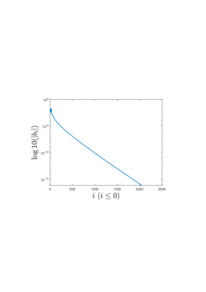
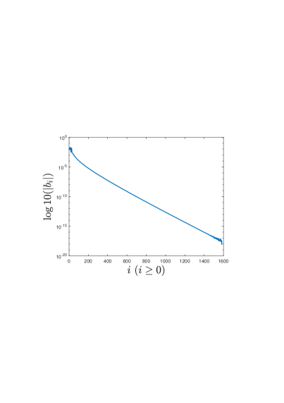
Figure 1: Toeplitz part of the computed $B=T(b)+E_{B}$ in Test 1: the log-scale of the absolute value of coefficients $b_{i}$ of the symbol $b(z)$ for $i\leq 0$ (left) and for $i\geq 0$ (right). The coefficients are computed by Algorithm 1.

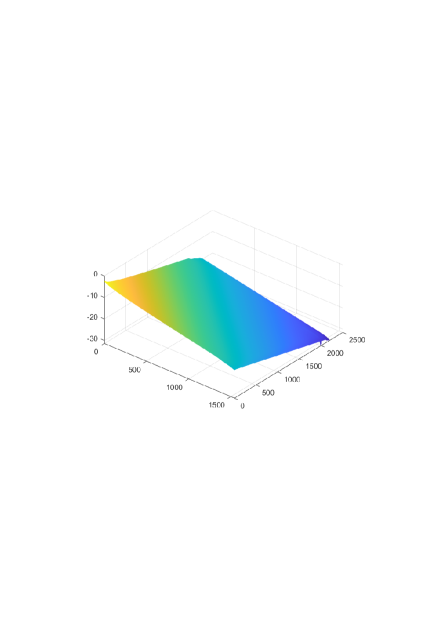
Figure 2: The correction part $E_{B}$ in Test 1: absolute value of $E_{B}$ in log scale, where $E_{B}$ is computed by the fixed-point iteration (5).

	Test 1			Test 2
Iterations	res.	iter.	time	res.	iter.	time
FPI	7.02e-14	55	114.77	9.62e-14	54	252.14
SDA	4.42e-14	6	170.07	6.61e-14	6	81.01

Table 1: Relative residual, number of iterations, CPU time in seconds in the computation $E_{B}$. FPI means the fixed-point iteration.

	Test 1	Test 2
Band	4200	376
Rows	2799	1296
Columns	1319	1162
Rank	80	1026

Table 2: Features of matrix $B=T(b)+E_{B}$ in Test 1 which is computed by FPI, including the band of the Toeplitz part $T(b)$, number of nonzero rows and columns, and rank of the correction of the computed $E_{B}$.

Example 5.2.

Let $A=I-S$ with $S=T(s)+E_{S}\in\mathcal{Q}\mathcal{T}_{\infty}$, where $T(s)=s_{0}I$ with $s_{0}<1$ and $E_{B}$ is the correction matrix with a $(p+m+n)\times(p+m+n)$ leading submatrix $E_{S}^{P}$ and zero elsewhere. Here, $E_{S}^{P}=\left(\begin{array}[]{ccc}V_{p}&&\\ &O_{m}&\\ &&-s_{0}I_{n}\end{array}\right)$, where $O_{m}$ is the zero matrix of size $m\times m$, $I_{n}$ is the identity matrix of size $n$, and the matrix $V_{p}=\left(\begin{array}[]{cc}U_{p\times q}\\ O_{(q-p)\times q}\end{array}\right)$ is a $q\times q$ block matrix with

$$U_{p\times q}=\left(\begin{array}[]{cccccc}u_{11}&u_{12}&\cdots&u_{1p}&\cdots&u_{1q}\\ 0&u_{22}&\cdots&u_{2p}&\cdots&u_{2q}\\ \vdots&\ddots&\ddots&\vdots&\ddots&\vdots\\ 0&0&\cdots&u_{pp}&\cdots&u_{pq}\end{array}\right)_{p\times q}.$$

where $u_{ii}=-s_{0}$ for $i=1,\ldots,p$, and $u_{i,j}\geq 0$ for $i=1,2,\ldots,p$ and $j=i+1\ldots,q$. Moreover, for $i=1,2,\ldots,p$, it satisfies that $\sum_{j=i+1}^{q}u_{ij}<1$.

Test	$s_{0}$	$m$	$n$	$p$	$q$
1	0.1	100	1000	1	100
2	0.5	100	1500	2	100
3	0.9	100	2000	2	100

Table 3: Different values of the parameters $s_{0},m,n,p$ and $q$.

For different values of the parameters $s_{0},m,n,p$ and $q$ as listed in Table 3, we apply the fixed-point iteration (5) and SDA to compute the matrix $E_{B}$ such that $(I-T(b)-E_{B})^{2}=A$. It can be seen that the symbol $b(z)$ satisfies $(1-b(z))^{2}=1-s_{0}$, which, together with the fact that $\|b\|_{{}_{{}_{\mathcal{W}}}}=\|T(b)\|_{\infty}<1$, implies $b(z)=1-\sqrt{1-s_{0}}$, so that $T(b)$ is a diagonal matrix with diagonal elements being $1-\sqrt{1-s_{0}}$.

In this example, we observe that $E_{B}$ can be obtained by the fixed-point iteration as well as SDA in just one or two steps. We also implement the Binomial iteration (BI) and the CR in [16] for computing the the whole matrix $B=T(b)+E_{B}$, the CPU time and residual error are compared with the fixed-point iteration and SDA in the computation of $E_{B}$, and are reported in Table 4. We mention that the residual error for BI and CR is obtained by $r=\|(I-\hat{Y})^{2}-A\|_{\infty}/\|A\|_{\infty}$, where $\hat{Y}$ is the computed square root.

	Test 1		Test 2		Test 3
Algorithms	time	res	time	res	time	res
FPI	2.7734	1.01e-15	19.44	3.00e-15	34.28	3.41e-14
SDA	8.4440	1.40e-15	25.25	2.35e-15	44.80	6.79e-14
CR	11.2681	1.83e-15	44.96	4.59e-15	95.91	7.48e-14
BI	14.3910	7.65e-16	48.40	2.02e-15	111.53	5.22e-14

Table 4: Comparison of the fixed-point iteration (5) and SDA in computing $E_{B}$ with the Binomial iteration and CR algorithm in computing $B$: the CPU time in seconds and relative residual in the computations.

As we can see from Table 4, the fixed-point iteration (5) and SDA take less CPU time comparing with the Binomial iteration and CR algorithm. Moreover, the fixed-point iteration (5), comparing with CR algorithm, has a speed-up in the CPU time by a factor of about 4 in Test 1 and 2.5 in Tests 2 and 3.

Example 5.3.

Let $A=cI-T(s)$ with $T(s)={\tt cqt(s_{n},s_{p})}$, where $c$, ${\tt s_{n}}$ and ${\tt s_{p}}$ are constructed in MATLAB as

${\tt s_{p}=rand(p,1)}$, ${\tt s_{n}=rand(q,1)}$, ${\tt s_{n}(1)=s_{p}(1)=1}$, ${\tt c=sum(s_{n})+sum(s_{p})}$.

It can be seen that $\|T(s)\|_{\infty}=\|s\|_{{}_{{}_{\mathcal{W}}}}<c$, so that $A$ is an invertible $M$-matrix. For different values of $p$ and $q$, we apply the fixed-point iteration (5) and SDA for computing matrix $E_{B}$ such that $c(I-T(b)-E_{B})^{2}=A$, where the symbol $b(z)$ is approximated by $\hat{b}(z)$ that is computed by Algorithm 1.

We also apply the fixed-point iteration and SDA to equation (19) for computing its solution $G$, so that $E_{B}$ can be approximated by extending $G$ to infinity. Table 5 reports the CPU time taken by the fixed-point iteration and SDA when applied to matrix equation (19), as well as the CPU time needed in the computation of the $E_{B}$ relying on the operations of quasi-Toeplitz matrices.

We observe from Table 5 that when the values of $p$ and $q$ are both small, say $p=4,q=2$, it seems that applying the fixed-point iteration (5) and SDA to the truncated matrix equation (19) takes less CPU time. For different values of $p$ and $q$ listed in Table 5, the rank of the correction matrix is $k$=501, 1539, 8496 and 3834, respectively, we observe that when $k$ becomes large, the algorithms applied to the truncated matrix equation (19) take more CPU times, and it can be seen that the algorithms relying on operations of quasi-Toeplitz matrices are more efficient.

($p,q$)	FPI	SDA
(4,2)	$2.79\cdot 10^{-2}$ $[1.09\cdot 10^{-1}]$	$1.95\cdot 10^{-2}$ $[1.13\cdot 10^{-1}]$
(12,10)	$4.19\cdot 10^{0}$ $[3.48\cdot 10^{0}]$	$2.45\cdot 10^{0}$ $[5.61\cdot 10^{0}]$
(20,2)	$6.90\cdot 10^{2}$ $[4.63\cdot 10^{1}]$	$6.56\cdot 10^{2}$ $[7.17\cdot 10^{1}]$
(20,20)	$7.52\cdot 10^{1}$ $[2.49\cdot 10^{1}]$	$3.53\cdot 10^{1}$ $[4.23\cdot 10^{1}]$

Table 5: CPU time in seconds, needed by the fixed-point iteration and SDA for computing a $k\times k$ matrix, which, after extending to infinity, is a good approximation to $E_{B}$. For comparison, the CPU time needed by FPI and SDA relying on the operations of quasi-Toeplitz matrices is written between bracket.

6 Conclusions

We have fully exploited the quasi-Toeplitz structure in the computation of the square root of invertible quasi-Toeplitz $M$-matrices. We propose algorithms for computing the Toeplitz part and the correction part respectively. The Toeplitz part is computed by Algorithm 1 at the basis of evaluation/interpolation at the $2n$ roots of unique. We propose a fixed-point iteration and a structure-preserving doubling algorithm for the computation of the correction part. Moreover, we show that the correction part can be approximated by extending the solution of a nonlinear matrix equation to infinity. Numerical experiments show that SDA in general takes less CPU time than the fixed-point iteration. There are also cases where the fixed-point iteration is inferior to SDA. There are cases where both the fixed-point iteration and SDA work better than the Binomial iteration and CR algorithm that exploit the quasi-Toeplitz structure indirectly.

References

- [1] G. Alefeld and N. Schneider. On square roots of -matrices, Linear Algebra Appl., 42 (1982) 119–132.
- [2] D. A. Bini, B. Iannazzo, and B. Meini. Numerical solution of algebraic Riccati equations, volume 9 of Fundamentals of Algorithms. Society for Industrial and Applied Mathematics (SIAM), Philadelphia, PA, 2012.
- [3] D. A. Bini, B. Iannazzo, and J. Meng. Geometric mean of quasi-Toeplitz matrices, arXiv preprint. 2021.
- [4] D. A. Bini, B. Iannazzo, B. Meini, J. Meng, and L. Robol. Computing eigenvalues of semi-infinite quasi-Toeplitz matrices. Numer. Algorithms, in press.
- [5] D. A. Bini, B. Iannazzo, and J. Meng, Algorithms for approximating means of semi-definite quasi-Toeplitz matrices, in: International Conference on Geometric Science of Information, GSI 2021: Geometric Science of Information, 2021, pp.405–414.
- [6] D. A. Bini, S. Massei, and B. Meini. Semi-infinite quasi-Toeplitz matrices with applications to QBD stochastic processes. Math. Comp., 87 (2018) 2811–2830.
- [7] D. A. Bini, S. Massei, and B. Meini. On functions of quasi Toeplitz matrices. Sb. Math., 208 (2017) 56–74.
- [8] D. A. Bini, S. Massei, B. Meini, and L. Robol. On quadratic matrix equations with infinite size coefficients encountered in QBD stochastic processes. Numer. Linear Algebra Appl., 25 (2018) e2128.
- [9] D. A. Bini, S. Massei, B. Meini, and L. Robol. A computational framework for two-dimensional random walks with restarts. SIAM J. Sci. Comput., 42(4) (2020) A2108–A2133.
- [10] D. A. Bini, S. Massei, and L. Robol. Quasi-Toeplitz matrix arithmetic: a MATLAB toolbox. Numer. Algorithms, 81 (2019) 741–769.
- [11] D. A. Bini, B. Meini, and J. Meng. Solving quadratic matrix equations arising in random walks in the quarter plane. SIAM J. Matrix Anal. Appl., 41 (2020) 691–714.
- [12] D. A. Bini and B. Meini. A defect-correction algorithm for quadratic matrix equations, with applications to quasi-Toeplitz matrices. arXiv preprint. 2022.
- [13] A. Bttcher and S. M. Grudsky. Spectral Properties of Banded Toeplitz Matrices. SIAM, Philadelphia, PA, 2005.
- [14] N. J. Higham, Functions of Matrices: Theory and Computation, Society for Industrial and Applied Mathematics, Philadelphia, PA, USA, 2008.
- [15] T.-M. Huang, R.-C. Li, and W.-W. Lin. Structure-preserving doubling algorithms for nonlinear matrix equations, volume 14 of Fundamentals of Algorithms. Society for Industrial and Applied Mathematics (SIAM), Philadelphia, PA, 2018.
- [16] J. Meng. Theoretical and computational properties of semi-infinite quasi-Toeplitz -matrices. Linear Algebra Appl., 653 (2022) 66–85.
- [17] R. V. Kadison and J. R. Ringrose. Fundamentals of the Theory of Operator Algebras. Vol. I, volume 100 of Pure and Applied Mathematics. Academic Press, Inc. [Harcourt Brace Jovanovich, Publishers], New York, 1983. Elementary theory.
- [18] M. R. Kannan and K. C. Sivakumar. On certain positivity classes of operators. Numerical Functional Analysis and Optimization, 37 (2017) 206–224.
- [19] I. Marek. Frobenius theory of positive operators: Comparison theorems and applications. SIAM J. Appl. Math., 19 (1970) 607–628.
- [20] I. Marek. On square roots of M-operators. Linear Algebra Appl., 223–224 (1995) 501–520.
- [21] I. Marek and D. B. Szyld. Splittings of -operators: Irreducibility and the index of the iteration operator. Numerical Functional Analysis and Optimization, 11 (1990) 529–553.
- [22] H.-M. Kim and J. Meng. Structured perturbation analysis for an infinite size quasi-Toeplitz matrix equation with applications. BIT Numerical Mathematics, 61 (2021) 859–879.
- [23] A. J. Motyer and P. G. Taylor. Decay rates for quasi-birth-and-death processes with countably many phases and tridiagonal block generators. Adv. Appl. Prob., 38 (2006) 522–544.
- [24] L. Robol. Rational Krylov and ADI iteration for infinite size quasi-Toeplitz matrix equations. Linear Algebra Appl., 604 (2020) 210–235.
- [25] P. N. Shivakumar, K. C. Sivakumar, and Y. Zhang. Infinite Matrices and Their Recent Applications, Springer International Publishing Switzerland, 2016.