Architecturing Binarized Neural Networks for Traffic Sign Recognition

Abstract

Traffic signs support road safety and managing the flow of traffic, hence are an integral part of any vision system for autonomous driving. While the use of deep learning is well-known in traffic signs classification due to the high accuracy results obtained using convolutional neural networks (CNNs) (state of the art is 99.46%), little is known about binarized neural networks (BNNs). Compared to CNNs, BNNs reduce the model size and simplify convolution operations and have shown promising results in computationally limited and energy-constrained devices which appear in the context of autonomous driving.

This work presents a bottom-up approach for architecturing BNNs by studying characteristics of the constituent layers. These constituent layers (binarized convolutional layers, max pooling, batch normalization, fully connected layers) are studied in various combinations and with different values of kernel size, number of filters and of neurons by using the German Traffic Sign Recognition Benchmark (GTSRB) for training. As a result, we propose BNNs architectures which achieve more than $90\%$ for GTSRB (the maximum is $96.45\%$) and an average greater than $80\%$ (the maximum is $88.99\%$) considering also the Belgian and Chinese datasets for testing. The number of parameters of these architectures varies from 100k to less than 2M. The accompanying material of this paper is publicly available at https://github.com/apostovan21/BinarizedNeuralNetwork.

1 Introduction

Traffic signs are important both in city and highway driving for supporting road safety and managing the flow of traffic. Therefore, traffic sign classification (recognition) is an integral part of any vision system for autonomous driving. It consists of: a) isolating the traffic sign in a bounding box, and b) classifying the sign into a specific traffic class. This work focuses on the second task.

Building a traffic sign classifier is challenging as it needs to cope with complex real-world traffic scenes. A well-know problem of the classifiers is the lack of robustness to adversarial examples [29] and to occlusions [30]. Adversarial examples are traffic signs taken as input which produce erroneous outputs and, together with occlusions, they naturally occur because the traffic scenes are unique in terms of weather conditions, lighting, aging.

One way to alleviate the lack of robustness is to formally verify that the trained classifier is robust to adversarial and occluded examples. For constructing the trained model, binary neural networks (BNNs) have shown promising results [14] even in computationally limited and energy-constrained devices which appear in the context of autonomous driving. BNNs are neural networks (NNs) with weights and/or activations binarized and constrained to $\pm 1$. Compared to NNs, they reduce the model size and simplify convolution operations utilized in image recognition task.

Our long term goal, which also motivated this work, is to give formal guarantees of properties (e.g. robustness) which are true for a trained classifier. The formal verification problem is formulated as follows: given a trained model and a property to be verified for the model, does the property hold for that model? To do so, the model and the property are translated into a constrained satisfaction problem and use, in principle, existing tools to solve the problem [22]. However, the problem is NP-complete [17], so experimentally beyond the reach of general-purpose tool.

This work makes an attempt to arrive at BNN architectures specifically for traffic signs recognition by making an extensive study of variation in accuracy, model size and number of parameters of the produced architectures. In particular, we are interested in BNNs architectures with high accuracy and small model size in order to be suitable in computationally limited and energy-constrained devices but, at the same time, reduced number of parameters in order to make the verification task easier. A bottom-up approach is adopted to design the architectures by studying characteristics of the constituent layers of internal blocks. These constituent layers are studied in various combinations and with different values of kernel size, number of filters and of neurons by using the German Traffic Sign Recognition Benchmark (GTSRB) for training. For testing, similar images from GTSRB, as well as from Belgian and Chinese datasets were used.

As a result of this study, we propose the network architectures (see Section 6) which achieve more than $90\%$ for GTSRB  [13] and an average greater than $80\%$ considering also the Belgian [1] and Chinese [3] datasets, and for which the number of parameters varies from 100k to 2M.

2 Related Work

Traffic Sign Recognition using CNNs. Traffic sign recognition (TSR) consists in predicting a label for the input based on a series of features learned by the trained classifier. CNNs were used in traffic sign classification since long time ago [27, 8]. These works used GTSRB [13] which is maintained and used on a large scale also nowadays. Paper [8] obtained an accuracy of 99.46% on the test images which is better than the human performance of 98.84%, while [27] with 98.31% was very close. These accuracies were obtained either modifying traditional models for image recognition (e.g. ResNet in case of [27]) or coming up with new ones (e.g. multi-column deep neural network composed of 25 CNNs in case of [8]). The architecture from [8] (see Figure 1) contains a number of parameters much higher than those of the models trained by us and it is not amenable for verification although the convolutional layers would be quantized. The work of [8] is still state of the art for TSR using CNNs.

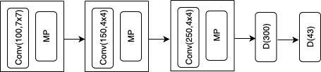
Figure 1: Architecture for recognizing traffic signs  [8]. Image sz: 48$\times$48  (px $\times$ px)

Binarized Neural Networks Architectures. Quantized neural networks (QNNs) are neural networks that represent their weights and activations using low-bit integer variables. There are two main strategies for training QNNs: post-training quantization and quantization-aware training [18] (QAT). The drawback of the post-training quantization is that it typically results in a drop in the accuracy of the network with a magnitude that depends on the specific dataset and network architecture. In our work, we use the second approach which is implemented in Larq library [11]. In QAT, the imprecision of the low-bit fixed-point arithmetic is modeled already during the training process, i.e., the network can adapt to a quantized computation during training. The challenge for QNNs is that they can not be trained directly with stochastic gradient descent (SGD) like classical NNs. This was solved by using the straight-through gradient estimator (STE) approach [15] which, in the forward pass of a training step, applies rounding operations to computations involved in the QNN (i.e. weights, biases, and arithmetic operations) and in the backward pass, the rounding operations are removed such that the error can backpropagate through the network.

BinaryConnect [9] is one of the first works which uses 1-bit quantization of weights during forward and backward propagation, but not during parameter update to maintain accurate gradient calculation during SGD. As an observation, the models used in conjuction with BinaryConnect use only linear layers which is suficient for MNIST [20] dataset, but convolutional layers for CIFAR-10 [19] and SVHN [24]. Paper [14] binarizes the activations as well. Similarly, for MNIST dataset they use linear layers, while for CIFAR-10, SVHN and ImageNet [10] they use variants of ConvNet, inspired by VGG [28], with the binarization of the activations.

In XNOR-Net [25], both the weights and the inputs to the convolutional and fully connected layers are approximated with binary values which allows an efficient way of implementing convolutional operations. The paper uses ImageNet dataset in experiments. We use XNOR-Net architectures in our work but for a new dataset, namely traffic signs.

Research on BNNs for traffic sign detection and recognition is scarce. Paper [7] uses the binarization of RetinaNet [21] and ITA [6] for traffic sign detection, in the first phase, and then recognition. Differently, we focus only on recognition, hence the architectures used have different underlying principles.

Verification of Neural Networks. Properties of neural networks are subject to verification. In the latest verification competition there are various benchmarks subject to verification [2], however, there is none involving traffic signs. This is because a model with reasonable accuracy for classification task must contain convolutional layers which leads to an increase of number of parameters. To the best of our knowledge there is only one paper which deals with traffic signs datasets [12] that is GTSRB. However, they considered only subsets of the dataset and their trained models consist of only fully connected layers with ReLU activation functions ranging from 70 to 1300. They do not mention the accuracy of their trained models. BNNs [23, 5] are also subject to verification but we did not find works involving traffic signs datasets.

3 Binarized Neural Networks

A BNN [14] is a feedforward network where weights and activations are mainly binary. [23] describes BNNs as sequential composition of blocks, each block consisting of linear and non-linear transformations. One could distinguish between internal and output blocks.

There are typically several internal blocks. The layers of the blocks are chosen in such a way that the resulting architecture fulfills the requirements of accuracy, model size, number of parameters, for example. Typical layers in an internal block are: 1) linear transformation (LIN), 2) binarization (BIN), 3) max pooling (MP), 4) batch normalization (BN). A linear transformation of the input vector can be based on a fully connected layer or a convolutional layer. In our case is a convolution layer since our experiments have shown that a fully connected layer can not synthesize well the features of traffic signs, therefore, the accuracy is low. The linear transformation is followed either by a binarization or a max pooling operation. Max pooling helps in reducing the number of parameters. One can swap binarization with max pooling, the result would be the same. We use this sequence as Larq [11], the library we used in our experiments, implements convolution and binarization in the same function. Finally, scaling is performed with a batch normalization operation [16].

There is one output block which produces the predictions for a given image. It consists of a dense layer that maps its input to a vector of integers, one for each output label class. It is followed by function which outputs the index of the largest entry in this vector as the predicted label.

We make the observation that, if the MP and BN layers are omitted, then the input and output of the internal blocks are binary, in which case, also the input to the output block. The input of the first block is never binarized as it drops down drastically the accuracy.

4 Datasets and Experimental Setting

We use GTSRB [4] for training and testing purposes of various architectures of BNNs. These architectures were also tested with the Belgian data set [1] and the Chinese [3].

GTSRB is a multi-class, single-image dataset. The dataset consists of images of German road signs in 43 classes, ranging in size from 25 $\times$ 25 to 243 $\times$ 225, and not all of them are square. Each class comprises 210 to 2250 images including prohibitory signs, danger signs, and mandatory signs. The training set contains 39209 images; the remaining 12630 images are selected as the testing set. For training and validation the ratio 80:20 was applied to the images in the train dataset. GTSRB is a challenging dataset even for humans, due to perspective change, shade, color degradation, lighting conditions, just to name a few.

The Belgium Traffic Signs test dataset contains 7095 images of 62 classes out of which only 23 match the ones from GTSRB. From that dataset we have used only the images from training folder which are 4533 in total. The Chinese Traffic Signs test dataset contains 5998 traffic sign images for testing of 58 classes out of which only 15 match the ones from GTSRB. For our experiments, we performed the following pre-processing steps on the Belgium and Chinese datasets, otherwise the accuracy of the trained model would be very low: 1) we relabeled the classes from the Belgium, respectively Chinese, datasets such that their common classes with GTSRB have the same label, and 2) we eliminated the classes not appearing in GTSRB.

In the end, for testing, we have used 1818 images from the Belgium dataset and 1590 from the Chinese dataset.

For this study, the following points are taken into consideration.

1. Training of network is done on Intel Iris Plus Graphics 650 GPU using Keras v2.10.0, Tensorflow v2.10.0 and Larq v0.12.2.

2. From the open-source Python library Larq [11], we used the function
   QuantConv2D in order to binarize the convolutional layers except the first. Subsequently, we denote it by QConv. The bias is set to False as we observed that does not influence negatively the accuracy but it reduces the number of parameters.

3. Input shape is fixed either to $30\times 30$, $48\times 48$, or $64\times 64$ (px $\times$ px). Due to lack of space, most of the experimental results included are for $30\times 30$, however all the results are available at https://github.com/apostovan21/BinarizedNeuralNetwork.

4. Unless otherwise stated, the number of epochs used in training is $30$.

5. Throughout the paper, for max pooling, the kernel is fixed to non-overlapping $2\times 2$ dimension.

6. Accuracy is measured with variation in the number of layers, kernel size, the number of filters and of neurons of the internal dense layer. Various combination of the following values considered are: (a) Number of blocks: $2,3,4$; (b) Kernel size: $2,3,5$; (c) Number of filters: $16,32,64,128,256$; (d) Number of neurons of the internal dense layer: $0,64,128,256,512,1024$.

7. ADAM is chosen as the default optimizer for this study. For initial training of deep learning networks, ADAM is the best overall choice [26].

Following section discusses the systematic progress of the study.

5 Proposed Methodology

We recall that the goal of our work is to obtain a set of architectures for BNNs with high accuracy but at the same time with small number of parameters for the scalability of the formal verification. At this aim, we proceed in two steps. First, we propose two simple two internal blocks XNOR architectures (Section 5.1). We train them on a set of images from GTSRB dataset and test them on similar images from the same dataset. We learned that MP reduces drastically the accuracy while the composition of a convolutional and binary layers (QConv) learns well the features of traffic signs images. In Section 5.2.1, we restore the accuracy lost by adding a BN layer after the MP one. At the same time, we try to increase the accuracy of the architecture composed by blocks of the QConv layer only by adding a BN layer after it.

Second, based on the learnings from Sections 5.1 and 5.2.1, as well as on the fact that a higher number of internal layers typically increases the accuracy, we propose several architectures (Section 5.2.2). Notable are those with accuracy greater than $90\%$ for GTSRB and an average greater than $80\%$ considering also the Belgian and Chinese datasets, and for which the number of parameters varies from 100k to 2M.

5.1 XNOR Architectures

We consider the two XNOR architectures from Figure 2. Each is composed of two internal blocks and an output dense (fully connected) layer. Note that, these architectures have only binary parameters. For the GTSRB, the results are in Table 1. One could observe that a simple XNOR architecture gives accuracy of at least $70\%$ as long as MP layers are not present but the number of parameters and the model size are high. We can conclude that QConv synthesizes the features well. However, MP layers reduce the accuracy tremendously.

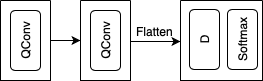
(a) XNOR(QConv) architecture

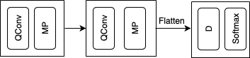
(b) XNOR(QConv,MP) architecture

Figure 2: XNOR architectures

Table 1: XNOR(QConv) and XNOR(QConv, MP) architectures. Image size: 30px $\times$ 30px. Dataset for train and test: GTSRB.

Model description	Acc	#Binary Params	Model Size (in KiB)
			Binary	Float-32
QConv(32, 3$\times$3), QConv(64, 2$\times$2), D(43)	77,91	2015264	246,5	7874,56
QConv(32, 3$\times$3), MP(2$\times$2), QConv(64, 2$\times$2), MP(2$\times$2), D(43)	5,46	108128	13,2	422,38
QConv(64, 3$\times$3), QConv(128, 2$\times$2), D(43)	70,05	4046912	495,01	15810,56
QConv(64, 3$\times$3), MP(2$\times$2), QConv(128, 2$\times$2), MP(2$\times$2) D(43)	10,98	232640	28,4	908,75
QConv(16, 3$\times$3), QConv(32, 2$\times$2), D(43)	81,54	1005584	122,75	3932,16
QConv(16, 3$\times$3), MP(2$\times$2), QConv(32, 2$\times$2), MP(2$\times$2), D(43)	1,42	52016	6,35	203,19

5.2 Binarized Neural Architectures

5.2.1 Two internal blocks

As of Table 1, the number of parameters for an architecture with MP layers is at least 15 times less than in a one without, while the size of the binarized models is approx. 30 times less than the 32 bits equivalent. Hence, to benefit from these two sweet spots, we propose a new architecture (see Figure 3(b)) which adds a BN layer in the second block of the XNOR architecture from Figure 2(b). The increase in accuracy is considerable (see Table 2). However, a BN layer following a binarized convolution (see Figure 3(a)) typically leads to a decrease in accuracy (see Table 3). The BN layer introduces few real parameters in the model as well as a slight increase in the model size. This is because only one BN layer was added. Note that the architectures from Figure 3 are not XNOR architectures.

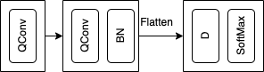
(a) XNOR(QConv) modified

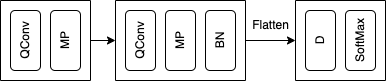
(b) XNOR(QConv, MP) enhanced

Figure 3: BNNs architectures which are not XNOR

Table 2: XNOR(QConv, MP) enhanced. Image size: 30px $\times$30px. Dataset for train and test: GTSRB.

		#Params			Model Size (in KiB)
Model description	Acc	Binary	Real	Total	Binary	Float-32
QConv(32, 3$\times$3), MP(2$\times$2), QConv(64, 2$\times$2), MP(2$\times$2), BN, D(43)	50,87	108128	128	108256	13,7	422,88
QConv(64, 3$\times$3), MP(2$\times$2), QConv(128, 2$\times$2), MP(2$\times$2), BN, D(43)	36,96	232640	256	232896	29,4	909,75
QConv(16, 3$\times$3), MP(2$\times$2), QConv(32, 2$\times$2), MP(2$\times$2), BN, D(43)	39,55	52016	64	52080	6,6	203,44

Table 3: XNOR(QConv) modified. Image size: 30px $\times$ 30px. Dataset for train and test: GTSRB.

Model description	Acc	#Params			Model Size (in KiB)
		Binary	Real	Total	Binary	Float-32
QConv(32, 3$\times$3), QConv(64, 2$\times$2), BN, D(43)	82,01	2015264	128	2015392	246,5	7874,56
QConv(64, 3$\times$3), QConv(128, 2$\times$2), BN, D(43)	69,12	4046912	256	4047168	495,01	15810,56
QConv(16, 3$\times$3), QConv(32, 2$\times$2), BN, D(43)	73,11	1005584	64	1005648	123	3932,16

5.2.2 Several Internal Blocks

Based on the results obtained in Sections 5.1 and 5.2.1, firstly, we trained an architecture where each internal block contains a BN layer only after the MP (see Figure 4(a)). This is based on the results from Tables 2 (the BN layer is crucial after MP for accuracy) and 3 (BN layer after QConv degrades the accuracy). There is an additional internal dense layer for which the number of neurons varies in the set $\{64,128,256,512,1028\}$. The results are in Table 4. One could observe that the conclusions drawn from the $2$ blocks architecture do not persist. Hence, motivated also by [14] we propose the architecture from Figure 4(b).

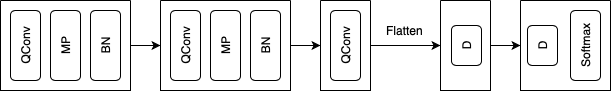
(a) 4-blocks Binarized Neural Architecture

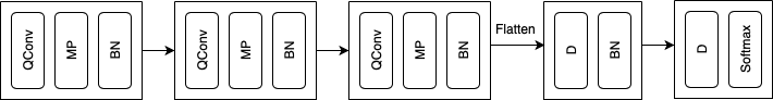
(b) Accuracy-efficient Binarized Neural Architectures

Figure 4: Binarized Neural Architectures

Table 4: Results for the architecture from the column Model Description. Image size: 30px $\times$30px. Dataset for train and test: GTSRB.

Model Description	#Neur	#Ep	Acc	#Params			Model size (in KiB)
				Binary	Real	Total	Binary	Float-32
QConv(32, 5x5), MP(2x2), BN, QConv(64, 5x5), MP(2x2), BN, QConv(64, 3x3), D(#Neur), D(43)	0	30	41,17	101472	192	101664	13,14	397,12
		100	52,17
	64	30	4,98	109600	192	109792	14,13	428,88
		100	5,70
	128	30	7,03	128736	192	128928	16,46	503,62
		100	5,70
	256	30	12,43	167008	192	167200	21,14	653,12
		100	8,48
	512	30	19,82	243552	192	243744	30,48	952,12
		100	32,13
	1024	30	46,05	396640	192	396832	49,17	1546,24
		100	50,91

6 Experimental results and discussion

The best accuracy for GTSRB and Belgium datasets is $96,45$ and $88,17$, respectively, and was obtained for the architecture from Figure 5, with input size 64$\times$64 (see Table 5). The number of parameters is almost $2$M and the model size $225,67$ KiB (for the binary model) and $6932,48$ KiB (for the Float-32 equivalent). There is no surprise the same architecture gave the best results for GTSRB and Belgium since they belong to the European area.

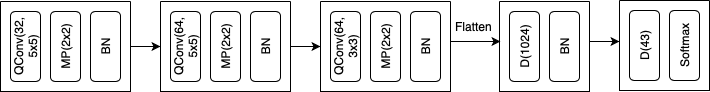
Figure 5: Accuracy Efficient Architecture for GTSRB and Belgium dataset

Table 5: Results for the architecture from Figure 5. Dataset for train: GTSRB.

Input size	#Neur	Accuracy			#Params			Model Size (in KiB)
		German	China	Belgium	Binary	Real	Total	Binary	Float-32
64px $\times$ 64px	0	93,83	77,86	79,75	159264	320	159584	20,69	623,38
	64	94,43	75,09	82,39	195616	448	196064	25,63	765,88
	128	95,42	74,71	83,44	300768	576	301344	38,96	1177,60
	256	94,75	80,37	81,40	511072	832	511904	65,64	1996,80
	512	95,65	78,49	85,64	931680	1344	933024	118,98	3645,44
	1024	96,45	81,50	88,17	1772896	2368	1775264	225,67	6932,48

The best accuracy for Chinese dataset ($83,9\%$) is obtained by another architecture, namely from Figure 6, with input size 48$\times$48 (see Table 6). This architecture is more efficient from the point of view of computationally limited devices and formal verification having $900$k parameters and $113,64$ KiB (for the binary model) and $3532,8$ KiB (for the Float-32 equivalent). Also, the second architecture gave the best average accuracy and the decrease in accuracy for GTSRB and Belgium is small, namely $1,17\%$ and $0,39\%$, respectively.

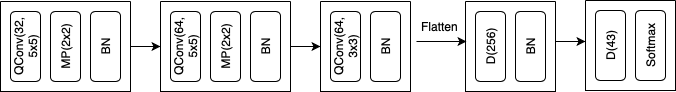
Figure 6: Accuracy Efficient Architecture for Chinese dataset

Table 6: Results for the architecture from Figure 6. Dataset for train: GTSRB.

Input size	#Neur	Accuracy			#Params			Model Size (in KiB)
		German	China	Belgium	Binary	Real	Total	Binary	Float-32
48px $\times$ 48px	0	94,67	82,13	83,16	225312	320	225632	28,75	881,38
	64	94,56	82,38	85,75	293920	448	294368	37,63	1146,88
	128	95,02	81,50	87,45	497376	576	497952	62,96	1945,60
	256	95,28	83,90	87,78	904288	832	905120	113,64	3532,80
	512	95,90	76,22	87,34	1718112	1344	1719456	214,98	6717,44
	1024	95,37	81,76	86,74	3345760	2368	3348128	417,67	13076,48

If we investigate both architectures based on confusion matrix results, for GTSRB we observe that the model failed to predict, for example, the End of speed limit 80 and Bicycle Crossing. The first was confused the most with Speed limit (80km/h), the second with Children crossing. One reason for the first confusion could be that End of speed limit (80 km/h) might be considered the occluded version of Speed limit (80km/h).

For Belgium test set, the worst results were obtained, for example, for Bicycle crossing and Wild animals crossing because the images differ a lot from the images on GTSRB training set (see Figure 7(a)). Another bad prediction is for Double Curve which was equally confused with Slippery road and Children crossing.

In the Chinese test set, the Traffic signals failed to be predicted at all by the model proposed by us and was assimilated with the General Caution class from the GTSRB, however General Caution is not a class in the Chinese test set (see Figure 7(b), top). Another bad prediction is for Speed limit (80km/h) which was equally confused with Speed limit (30km/h), Speed limit (50km/h) and Speed limit (60km/h) but not with Speed limit (70km/h). One reason could be the quality of the training images compared to the test ones (see Figure 7(b), bottom).

In conclusion, there are few cases when the prediction failures can be explained, however the need for formal verification guarantees of the results is urgent which we will be performed as future work.

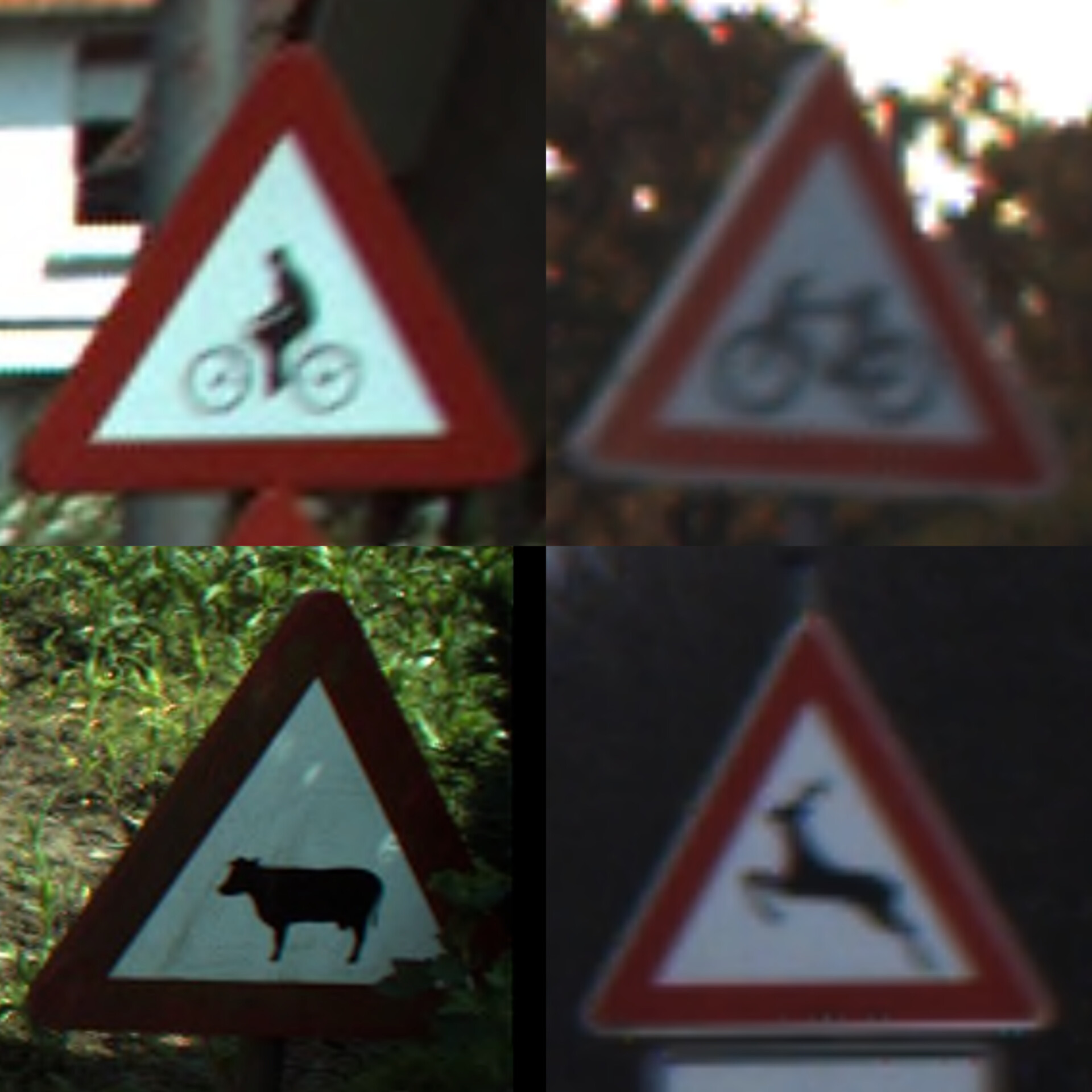
(a) Difference between Belgium (left) and GRSRB (right) dataset

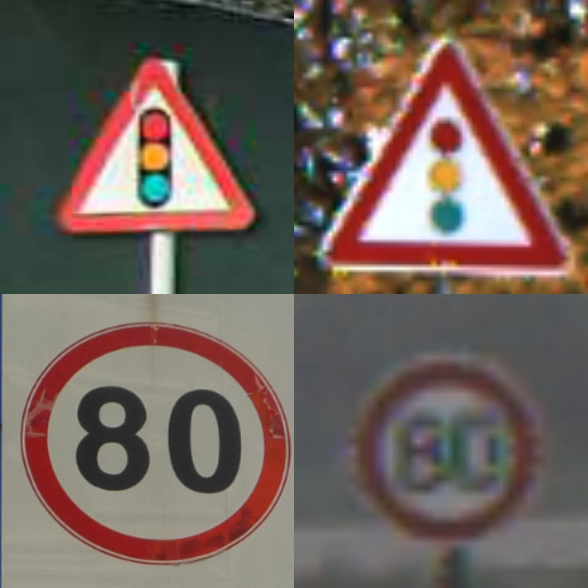
(b) Difference between Chinese (left) and GRSRB (right) dataset

Figure 7: Differences between traffic sign in the datasets

References

- [1] Belgian Traffic Sign Database. https://www.kaggle.com/datasets/shazaelmorsh/trafficsigns, accessed: March 25th, 2023
- [2] Benchmarks of the 3rd International Verification of Neural Networks Competition (VNN-COMP’22). https://github.com/ChristopherBrix/vnncomp2022_benchmarks, accessed: February 22nd, 2023
- [3] Chinese Traffic Sign Database. https://www.kaggle.com/datasets/dmitryyemelyanov/chinese-traffic-signs, accessed: March 25th, 2023
- [4] German Traffic Sign Recognition Benchmark. https://www.kaggle.com/datasets/meowmeowmeowmeowmeow/gtsrb-german-traffic-sign?datasetId=82373&language=Python, accessed: March 25th, 2023
- [5] Amir, G., Wu, H., Barrett, C., Katz, G.: An SMT-based Approach for Verifying Binarized Neural Networks. In: Tools and Algorithms for the Construction and Analysis of Systems: 27th International Conference, TACAS 2021, Held as Part of the European Joint Conferences on Theory and Practice of Software, ETAPS 2021, Luxembourg City, Luxembourg, March 27–April 1, 2021, Proceedings, Part II 27. pp. 203–222. Springer (2021)
- [6] Chen, E.H., Röthig, P., Zeisler, J., Burschka, D.: Investigating Low Level Features in CNN for Traffic Sign Detection and Recognition. In: 2019 IEEE Intelligent Transportation Systems Conference (ITSC). pp. 325–332. IEEE (2019)
- [7] Chen, E.H., Vemparala, M.R., Fasfous, N., Frickenstein, A., Mzid, A., Nagaraja, N.S., Zeisler, J., Stechele, W.: Investigating Binary Neural Networks for Traffic Sign Detection and Recognition. In: 2021 IEEE Intelligent Vehicles Symposium (IV). pp. 1400–1405. IEEE (2021)
- [8] Ciregan, D., Meier, U., Schmidhuber, J.: Multi-Column Deep Neural Networks for Image Classification. In: 2012 IEEE conference on computer vision and pattern recognition. pp. 3642–3649. IEEE (2012)
- [9] Courbariaux, M., Bengio, Y., David, J.P.: BinaryConnect: Training Deep Neural Networks with Binary Weights during Propagations. Advances in neural information processing systems 28 (2015)
- [10] Deng, J., Dong, W., Socher, R., Li, L.J., Li, K., Fei-Fei, L.: ImageNet: A Large-Scale Hierarchical Image Database. In: 2009 IEEE conference on computer vision and pattern recognition. pp. 248–255. Ieee (2009)
- [11] Geiger, L., Team, P.: Larq: An Open-Source Library for Training Binarized Neural Networks. Journal of Open Source Software 5(45), 1746 (2020)
- [12] Guo, X., Zhou, Z., Zhang, Y., Katz, G., Zhang, M.: OccRob: Efficient SMT-Based Occlusion Robustness Verification of Deep Neural Networks. arXiv preprint arXiv:2301.11912 (2023)
- [13] Houben, S., Stallkamp, J., Salmen, J., Schlipsing, M., Igel, C.: Detection of Traffic Signs in Real-World Images: The German Traffic Sign Detection Benchmark. In: The 2013 international joint conference on neural networks (IJCNN). pp. 1–8. Ieee (2013)
- [14] Hubara, I., Courbariaux, M., Soudry, D., El-Yaniv, R., Bengio, Y.: Binarized Neural Networks. Advances in neural information processing systems 29 (2016)
- [15] Hubara, I., Courbariaux, M., Soudry, D., El-Yaniv, R., Bengio, Y.: Quantized Neural Networks: Training Neural Networks with Low Precision Weights and Activations. The Journal of Machine Learning Research 18(1), 6869–6898 (2017)
- [16] Ioffe, S., Szegedy, C.: Batch Normalization: Accelerating Deep Network Training by Reducing Internal Covariate Shift. In: International conference on machine learning. pp. 448–456. PMLR (2015)
- [17] Katz, G., Barrett, C., Dill, D.L., Julian, K., Kochenderfer, M.J.: Reluplex: An Efficient SMT Solver for Verifying Deep Neural Networks. In: Computer Aided Verification: 29th International Conference, CAV 2017, Heidelberg, Germany, July 24-28, 2017, Proceedings, Part I 30. pp. 97–117. Springer (2017)
- [18] Krishnamoorthi, R.: Quantizing Deep Convolutional Networks for Efficient Inference: A whitepaper. arXiv preprint arXiv:1806.08342 (2018)
- [19] Krizhevsky, A., Hinton, G., et al.: Learning Multiple Layers of Features from Tiny Images (2009)
- [20] LeCun, Y.: The MNIST Database of Handwritten Digits. http://yann. lecun. com/exdb/mnist/ (1998)
- [21] Lin, T.Y., Goyal, P., Girshick, R., He, K., Dollár, P.: Focal Loss for Dense Object Detection. In: Proceedings of the IEEE international conference on computer vision. pp. 2980–2988 (2017)
- [22] de Moura, L., Bjørner, N.: Z3: An Efficient SMT Solver. In: Ramakrishnan, C.R., Rehof, J. (eds.) Tools and Algorithms for the Construction and Analysis of Systems. pp. 337–340. Springer Berlin Heidelberg, Berlin, Heidelberg (2008)
- [23] Narodytska, N.: Formal Analysis of Deep Binarized Neural Networks. In: IJCAI. pp. 5692–5696 (2018)
- [24] Netzer, Y., Wang, T., Coates, A., Bissacco, A., Wu, B., Ng, A.Y.: Reading Digits in Natural Images with Unsupervised Feature Learning (2011)
- [25] Rastegari, M., Ordonez, V., Redmon, J., Farhadi, A.: XNOR-Net: ImageNet Classification using Binary Convolutional Neural Networks. In: European conference on computer vision. pp. 525–542. Springer (2016)
- [26] Ruder, S.: An Overview of Gradient Descent Optimization Algorithms. arXiv preprint arXiv:1609.04747 (2016)
- [27] Sermanet, P., LeCun, Y.: Traffic Sign Recognition with Multi-Scale Convolutional Networks. In: The 2011 international joint conference on neural networks. pp. 2809–2813. IEEE (2011)
- [28] Simonyan, K., Zisserman, A.: Very Deep Convolutional Networks for Large-Scale Image Recognition. arXiv preprint arXiv:1409.1556 (2014)
- [29] Szegedy, C., Zaremba, W., Sutskever, I., Bruna, J., Erhan, D., Goodfellow, I., Fergus, R.: Intriguing Properties of Neural Networks. arXiv preprint arXiv:1312.6199 (2013)
- [30] Zhang, J., Wang, W., Lu, C., Wang, J., Sangaiah, A.K.: Lightweight Deep Network for Traffic Sign Classification. Annals of Telecommunications 75, 369–379 (2020)