On CNF Conversion for SAT and SMT Enumeration

Abstract

Modern SAT and SMT solvers are designed to handle problems expressed in Conjunctive Normal Form (CNF) so that non-CNF problems must be CNF-ized upfront, typically by using variants of either Tseitin or Plaisted and Greenbaum transformations. When passing from solving to enumeration, however, the capability of producing partial satisfying assignments that are as small as possible becomes crucial, which raises the question of whether such CNF encodings are also effective for enumeration.

In this paper, we investigate both theoretically and empirically the effectiveness of CNF conversions for SAT and SMT enumeration. On the negative side, we show that: (i) Tseitin transformation prevents the solver from producing short partial assignments, thus seriously affecting the effectiveness of enumeration; (ii) Plaisted and Greenbaum transformation overcomes this problem only in part. On the positive side, we prove theoretically and we show empirically that combining Plaisted and Greenbaum transformation with NNF preprocessing upfront —which is typically not used in solving— can fully overcome the problem and can drastically reduce both the number of partial assignments and the execution time.

1 Introduction

State-of-the-art SAT and SMT solvers deal very efficiently with formulas expressed in Conjunctive Normal Form (CNF). In real-world scenarios, however, it is common for problems to be expressed as non-CNF formulas. Hence, these problems are converted into CNF before being processed by the solver. This conversion is generally done by using variants of the ? (?) or the ? (?) transformations, which generate a linear-size equisatisfiable CNF formula by labelling sub-formulas with fresh Boolean atoms. These transformations can be employed also for SAT and SMT enumeration (AllSAT and AllSMT, respectively), by projecting the truth assignments onto the original atoms only.

When passing from solving to enumeration, however, the capability of enumerating partial satisfying assignments that are as small as possible is crucial, because each prevents from enumerating a number of total assignments that is exponential w.r.t. the number of unassigned atoms. This raises the question of whether CNF encodings conceived for solving are also effective for enumeration. To the best of our knowledge, however, no research has yet been published to analyse how the different CNF encodings may affect the effectiveness of the solvers for AllSAT and AllSMT.

In this paper, we investigate, both theoretically and empirically, the effectiveness of CNF conversion for SAT and SMT enumeration, both in the disjoint and non-disjoint cases. The contribution of this paper is twofold.

First, on the negative side, we show that the commonly-employed CNF transformations for solving are not suitable for enumeration. In particular, we notice that the Tseitin encoding introduces top-level label definitions for sub-formulas with double implications, which need to be satisfied as well, and thus prevent the solver from producing short partial assignments. We also notice that the Plaisted and Greenbaum transformation solves this problem only in part by labelling sub-formulas only with single implications if they occur with single polarity, but it has similar issues to the Tseitin transformation when sub-formulas occur with both polarities.

Second, on the positive side, we prove theoretically and we show empirically that converting the formula into Negation Normal Form (NNF) before applying the Plaisted and Greenbaum transformation can fix the problem and drastically improve the effectiveness of the enumeration process by up to orders of magnitude.

This analysis is confirmed by an experimental evaluation of non-CNF problems originating from both synthetic and real-world-inspired applications. The results confirm the theoretical analysis, showing that the proposed combination of NNF with the Plaisted and Greenbaum CNF allows for a drastic reduction in both the number of partial assignments and the execution time.

Disclaimer.

A preliminary and much shorter version of this paper was presented at SAT 2023 (?). In this paper, we present the following novel contributions:

• we formalize the main claim of the paper and formally prove it (Theorem 1 in §4);

• we extend the analysis to non-disjoint AllSAT and to disjoint and non-disjoint AllSMT;

• we extend the empirical evaluation to a much broader set of benchmarks, including also non-disjoint AllSAT and disjoint and non-disjoint AllSMT, which confirm the theoretical results. Moreover, we extend the timeout of each job-pair from 1200s to 3600s, providing thus a more informative comparison;

• we present a much more detailed related work section.

Content.

The paper is organized as follows. In §2 we introduce the theoretical background necessary to understand the rest of the paper. In §3 we analyse the problem of the classical CNF-izations when used for AllSAT and AllSMT. In §4 we propose one possible solution, whose effectiveness is evaluated on both synthetic and real-world inspired benchmarks in §5. The related work is presented in §6. We conclude the paper in §7, drawing some final remarks and indicating possible future work.

2 Background

This section introduces the notation and the theoretical background necessary to understand what is presented in this paper. We assume the reader is familiar with the basic syntax, semantics and results of propositional and first-order logics. We briefly summarize the main concepts and results of SAT and SMT, and the fundamental ideas behind SAT and SMT enumeration and projected enumeration implemented by modern AllSAT and AllSMT solvers.

2.1 SAT and SAT Modulo Theories

Notation.

In the paper, we adopt the following conventions. We refer to Boolean atoms with capital letters, such as $A$ and $B$, and to generic atoms, both Boolean and first-order, with Greek letters such as $\alpha$. The symbols $\mathbf{A}\stackrel{{\scriptstyle\text{\scalebox{0.7}{def}}}}{{=}}\{{A_{1},\dots,A_{N}}\}$ and $\mathbf{B}\stackrel{{\scriptstyle\text{\scalebox{0.7}{def}}}}{{=}}\{{B_{1},\dots,B_{M}}\}$ denote disjoint sets of Boolean atoms, and $\boldsymbol{\alpha}{}\stackrel{{\scriptstyle\text{\scalebox{0.7}{def}}}}{{=}}\{{\alpha_{1},\dots,\alpha_{k}}\}$ denotes a set of generic Boolean or first-order atoms. Propositional and first-order formulas are referred to with Greek letters $\varphi,\psi$. We denote Boolean constants by $\mathbb{B}\stackrel{{\scriptstyle\text{\scalebox{0.7}{def}}}}{{=}}\{{\top,\bot}\}$. Total truth assignments are denoted by $\eta$, whereas partial truth assignments are denoted by $\mu$, possibly annotated with superscripts.

Propositional Satisfiability.

A propositional (also Boolean) formula $\varphi$ can be defined recursively as follows. The Boolean constants $\top$ and $\bot$ are formulas; a Boolean atom $A$ and its negation $\neg A$ are formulas, also referred to as literals; a connection of two formulas by one of the Boolean connectives $\wedge,\vee,\rightarrow,\leftrightarrow$ is a formula. A disjunction $(\vee)$ of literals is called a clause. A conjunction $(\wedge)$ of literals is called a cube. Propositional satisfiability (SAT) is the problem of deciding the satisfiability of a propositional formula.

Satisfiability Modulo Theories.

As it is standard in most SMT literature, we restrict to quantifier-free first-order formulas. A first-order term is either a variable, a constant symbol, or a combination of terms by means of function symbols. A first-order atom is a predicate symbol applied to a tuple of terms (Boolean atoms can be viewed as zero-arity predicates). A first-order formula is either a first-order atom, or a connection of two formulas by one of the Boolean connectives. A first-order theory $\mathcal{T}$ is a (possibly infinite) set of first-order formulas, that provides an intended interpretation of constant, function, and predicate symbols. Examples of theories of practical interest are those of equality and uninterpreted functions ($\mathcal{EUF}$), of linear arithmetic over integer ($\mathcal{LIA}$) or real numbers ($\mathcal{LRA}$), and combinations thereof. We refer to formulas and atoms over symbols defined by $\mathcal{T}$ as $\mathcal{T}$-formulas and $\mathcal{T}$-atoms, respectively.

Satisfiability Modulo the Theory $\mathcal{T}$, also $\text{SMT}(\mathcal{T})$, is the problem of deciding the satisfiability of a first-order formula with respect to some background theory $\mathcal{T}$. A formula $\varphi$ is $\mathcal{T}$-satisfiable if $\varphi\wedge\mathcal{T}{}$ is satisfiable in the first-order sense. Otherwise, it is $\mathcal{T}$-unsatisfiable. We refer to the work by ? (?) for details.

Hereafter, unless otherwise specified, by “formulas” we mean both Boolean and $\mathcal{T}$-formulas, and by “atoms” we mean both Boolean and $\mathcal{T}$-atoms, for a generic theory $\mathcal{T}$.

Total and partial truth assignments.

Given a set of atoms $\boldsymbol{\alpha}$, a total truth assignment is a total map $\eta:\boldsymbol{\alpha}\longmapsto\mathbb{B}$. A partial truth assignment is a partial map $\mu:\boldsymbol{\alpha}\longmapsto\mathbb{B}$. Notice that a partial truth assignment represents $2^{K}$ total truth assignments, where $K$ is the number of atoms unassigned by $\mu$. With a little abuse of notation, we sometimes represent a truth assignment either as a set, s.t. $\mu\stackrel{{\scriptstyle\text{\scalebox{0.7}{def}}}}{{=}}\{{\alpha\ |\ \mu(\alpha)=\top}\}\cup\{{\neg\alpha\ |\ \mu(\alpha)=\bot}\}$, or as a cube, s.t. $\mu\stackrel{{\scriptstyle\text{\scalebox{0.7}{def}}}}{{=}}\bigwedge_{\mu(\alpha)=\top}{\alpha}\wedge\bigwedge_{\mu(\alpha)=\bot}{\neg\alpha}$. If $\mu_{1}\subseteq\mu_{2}$ [resp. $\mu_{1}\subset\mu_{2}$] we say that $\mu_{1}$ is a sub-assignment [resp. strict sub-assignment] of $\mu_{2}$ and that $\mu_{2}$ is a super-assignment [resp. strict super-assignment] of $\mu_{1}$. We denote with $\varphi|_{\mu}$ the residual of $\varphi$ under $\mu$, i.e. the formula obtained by substituting in $\varphi$ each $\alpha_{i}\in\boldsymbol{\alpha}$ with $\mu(\alpha_{i})$, and by recursively applying the standard propagation rules of truth values through Boolean operators.

Given a set of atoms $\boldsymbol{\alpha}$ and a formula $\varphi(\boldsymbol{\alpha})$, we say that a [partial or total] truth assignment $\mu:\boldsymbol{\alpha}\longmapsto\mathbb{B}$ propositionally satisfies $\varphi$, denoted as $\mu\models_{p}\varphi$, iff $\varphi|_{\mu}=\top$. A partial truth assignment $\mu$ is minimal for $\varphi$ iff $\mu\models_{p}\varphi$ and every strict sub-assignment $\mu{}^{\prime}\subset\mu$ is such that $\mu{}^{\prime}\not\models_{p}\varphi$. A Boolean formula is satisfiable iff there exists a truth assignment propositionally satisfying it. A $\mathcal{T}$-formula is $\mathcal{T}$-satisfiable iff there exists a $\mathcal{T}$-satisfiable truth assignment propositionally satisfying it.

Given two disjoint sets of atoms $\boldsymbol{\alpha},\mathbf{B}$ and a formula $\psi(\boldsymbol{\alpha}\cup\mathbf{B})$, we say that a [partial or total] truth assignment $\mu^{\boldsymbol{\alpha}}:\boldsymbol{\alpha}\longmapsto\mathbb{B}$ propositionally satisfies $\exists\mathbf{B}.\psi$ iff there exists a total truth assignment $\eta^{\mathbf{B}}:\mathbf{B}\longmapsto\mathbb{B}$ such that $\mu^{\boldsymbol{\alpha}}\cup\eta^{\mathbf{B}}:\boldsymbol{\alpha}\cup\mathbf{B}\longmapsto\mathbb{B}$ propositionally satisfies $\psi$.

Two formulas $\varphi{}$ and $\psi{}$ are propositionally equivalent, denoted as $\varphi\equiv_{p}\psi$, iff every total truth assignment propositionally satisfying $\varphi$ also propositionally satisfies $\psi$, and vice versa.

Negation Normal Form.

Given a formula $\varphi$, a sub-formula occurs with positive [resp. negative] polarity (also positively [resp. negatively]) if it occurs under an even [resp. odd] number of nested negations. Specifically, $\varphi$ occurs positively in $\varphi$; if $\neg\varphi_{1}$ occurs positively [resp. negatively] in $\varphi$, then $\varphi_{1}$ occurs negatively [resp. positively] in $\varphi$; if $\varphi_{1}\wedge\varphi_{2}$ or $\varphi_{1}\vee\varphi_{2}$ occur positively [resp. negatively] in $\varphi$, then $\varphi_{1}$ and $\varphi_{2}$ occur positively [resp. negatively] in $\varphi$; if $\varphi_{1}\rightarrow\varphi_{2}$ occurs positively [resp. negatively] in $\varphi$, then $\varphi_{1}$ occurs negatively [resp. positively] and $\varphi_{2}$ occurs positively [resp. negatively] in $\varphi$; if $\varphi_{1}\leftrightarrow\varphi_{2}$ occurs in $\varphi$, then $\varphi_{1}$ and $\varphi_{2}$ occur both positively and negatively in $\varphi$.

A formula is in Negation Normal Form (NNF) iff it is given only by the recursive applications of $\wedge$ and $\vee$ to literals, i.e., iff all its sub-formulas occur positively, except for literals. An NNF formula can be conveniently represented as a Directed Acyclic Graph (DAG) —that is, as a single-root and/or DAG with literals as leaves. We call the size of an NNF DAG the sum of the numbers of its nodes and arcs. A formula can be converted into a propositionally-equivalent NNF formula by recursively rewriting implications $(\varphi_{1}\rightarrow\varphi_{2})$ as $(\neg\varphi_{1}\vee\varphi_{2})$ and equivalences $(\varphi_{1}\leftrightarrow\varphi_{2})$ as $(\neg\varphi_{1}\vee\varphi_{2})\wedge(\varphi_{1}\vee\neg\varphi_{2})$, and then by recursively “pushing down” the negations: $\neg(\varphi_{1}\vee\varphi_{2})$ as $(\neg\varphi_{1}\wedge\neg\varphi_{2})$, $\neg(\varphi_{1}\wedge\varphi_{2})$ as $(\neg\varphi_{1}\vee\neg\varphi_{2})$ and $\neg\neg\varphi_{1}$ as $\varphi_{1}$. The following fact holds.

Property 1.

Let $\varphi$ be a formula and $\mathsf{NNF}(\varphi)$ be the NNF formula resulting from converting $\varphi$ into NNF as described above. If $\mathsf{NNF}(\varphi)$ is represented as a DAG, then its size is linear w.r.t. the original one.

(Although we believe this fact is well-known, we provide a formal proof in Section A.1.) Intuitively, we only need at most 2 nodes for each sub-formula $\varphi_{i}$ of $\varphi$, representing $\mathsf{NNF}(\varphi_{i})$ and $\mathsf{NNF}(\neg\varphi_{i})$ for positive and negative occurrences of $\varphi_{i}$ respectively. These nodes are shared among up to exponentially-many branches generated by expanding the nested iffs.

We have the following fact, for which we provide a complete proof in Section A.2.

Property 2.

Consider a formula $\varphi$, and let $\mathsf{NNF}(\varphi)$ be its NNF DAG. Consider a partial truth assignment $\mu$. Then $\varphi|_{\mu}=v$ iff $\mathsf{NNF}(\varphi)|_{\mu}=v$, for $v\in\{{\top,\bot}\}$.

Notice that this is not a direct consequence of the fact that $\mathsf{NNF}(\varphi)$ is equivalence-preserving, because the above notion of satisfiability by partial assignment is such that if $\varphi_{1}\equiv_{p}\varphi_{2}$, then $\mu\models_{p}\varphi_{1}$ does not imply that $\mu\models_{p}\varphi_{2}$ (?, ?). E.g, consider $\varphi_{1}\stackrel{{\scriptstyle\text{\scalebox{0.7}{def}}}}{{=}}(A\vee{}B)\wedge(A\vee\neg{}B)$ and $\varphi_{2}\stackrel{{\scriptstyle\text{\scalebox{0.7}{def}}}}{{=}}(A\wedge{}B)\vee(A\wedge{\neg{}B})$, and the partial assignment $\mu\stackrel{{\scriptstyle\text{\scalebox{0.7}{def}}}}{{=}}\{{A}\}$. Although $\varphi_{1}\equiv_{p}\varphi_{2}$, we have that $\varphi_{1}|_{\mu}=\top$, but $\varphi_{2}|_{\mu}=B\vee\neg B$, which, although logically equivalent to $\top{}$, is syntactically different from it.

CNF Transformations.

A formula is in Conjunctive Normal Form (CNF) iff it is a conjunction of clauses. Numerous CNF transformation procedures, commonly referred to as CNF-izations, have been proposed in the literature. We summarize the three most frequently employed techniques.

The Classic CNF-ization ($\mathsf{CNF_{DM}}$) converts a formula into a propositionally-equivalent formula in CNF by applying DeMorgan’s rules. First, it converts the formula into NNF. Second, it recursively rewrites sub-formulas $\varphi_{1}\vee(\varphi_{2}\wedge\varphi_{3})$ as $(\varphi_{1}\vee\varphi_{2})\wedge(\varphi_{1}\vee\varphi_{3})$ to distribute $\vee$ over $\wedge$, until the formula is in CNF. The principal limitation of this transformation lies in the possible exponential growth of the resulting formula compared to the original (e.g., when the formula is a disjunction of conjunctions of sub-formulas), making it unsuitable for modern SAT and SMT solvers (see e.g., ?).

The Tseitin CNF-ization ($\mathsf{CNF_{Ts}}$) (?) avoids this exponential blow-up by labelling each sub-formula $\varphi_{i}$ with a fresh Boolean atom $B_{i}$, which is used as a placeholder for the sub-formula. Specifically, it consists in applying recursively bottom-up the rewriting rule $\varphi\Longrightarrow\varphi[\varphi_{i}|B_{i}]\wedge\mathsf{CNF_{DM}}(B_{i}\leftrightarrow\varphi_{i})$ until the resulting formula is in CNF, where $\varphi[\varphi_{i}|B_{i}]$ is the formula obtained by substituting in $\varphi$ every occurrence of $\varphi_{i}$ with $B_{i}$.

The Plaisted and Greenbaum CNF-ization ($\mathsf{CNF_{PG}}$) (?) is a variant of the $\mathsf{CNF_{Ts}}$ that exploits the polarity of sub-formulas to reduce the number of clauses of the final formula. Specifically, if a sub-formula $\varphi_{i}$ appears only with positive [resp. negative] polarity, then it can be labelled with a single implication as $\mathsf{CNF_{DM}}(B_{i}\rightarrow\varphi_{i})$ [resp. $\mathsf{CNF_{DM}}(B_{i}\leftarrow\varphi_{i})$].

With both $\mathsf{CNF_{Ts}}$ and $\mathsf{CNF_{PG}}$, due to the introduction of the label variables, the final formula does not preserve the propositional equivalence with the original formula but only the equisatisfiability. Moreover, they also have a stronger property. If $\varphi(\boldsymbol{\alpha})$ is a non-CNF formula and $\psi(\boldsymbol{\alpha}\cup\mathbf{B})$ is either the $\mathsf{CNF_{Ts}}$ or the $\mathsf{CNF_{PG}}$ encoding of $\varphi$, where $\mathbf{B}$ are the fresh Boolean atoms introduced by the transformation, then $\varphi(\boldsymbol{\alpha})\equiv_{p}\exists\mathbf{B}.\psi(\boldsymbol{\alpha}\cup\mathbf{B})$.

Most of the modern SAT and SMT solvers do not deal directly with non-CNF formulas, rather they convert them into CNF by using either $\mathsf{CNF_{Ts}}$ or $\mathsf{CNF_{PG}}$, and then find truth assignments propositionally satisfying $\varphi(\boldsymbol{\alpha})$ by finding truth assignments propositionally satisfying $\exists\mathbf{B}.\psi(\boldsymbol{\alpha}\cup\mathbf{B})$.

2.2 AllSAT, AllSMT, Projected AllSAT and Projected AllSMT

AllSAT is the task of enumerating all the truth assignments propositionally satisfying a propositional formula. The task can be found in the literature in two versions: disjoint AllSAT, in which the assignments are required to be pairwise mutually-inconsistent, and non-disjoint AllSAT, in which they are not. A generalization to the $\text{SMT}(\mathcal{T})$ case is All$\text{SMT}(\mathcal{T})$, defined as the task of enumerating all the $\mathcal{T}$-satisfiable truth assignments propositionally satisfying a $\text{SMT}(\mathcal{T})$ formula. Also in this case, both disjoint or non-disjoint All$\text{SMT}(\mathcal{T})$ are considered.

In the following, for the sake of compactness, we present definitions and algorithms referring to AllSAT. An extension to All$\text{SMT}(\mathcal{T})$ can be obtained straightforwardly, by substituting “$\mathbf{A}$” with “$\boldsymbol{\alpha}$” and “truth assignments” with “$\mathcal{T}$-satisfiable truth assignments”.

Given a formula $\varphi$, we denote with $\mathcal{T}\mathcal{T}\mathcal{A}(\varphi)\stackrel{{\scriptstyle\text{\scalebox{0.7}{def}}}}{{=}}\{{\eta_{1},\dots,\eta_{j}\dots\eta_{M}}\}$ the set of all total truth assignments propositionally satisfying $\varphi$. We denote with $\mathcal{T}\mathcal{A}(\varphi)\stackrel{{\scriptstyle\text{\scalebox{0.7}{def}}}}{{=}}\{{\mu_{1},\dots,\mu_{i}\dots,\mu_{N}}\}$ a set of partial truth assignments propositionally satisfying $\varphi$ s.t.:

1. every $\eta\in\mathcal{T}\mathcal{T}\mathcal{A}(\varphi)$ is a super-assignment of some $\mu\in\mathcal{T}\mathcal{A}(\varphi)$;

and, only in the disjoint case:

1. every pair $\mu_{i},\mu_{j}\in\mathcal{T}\mathcal{A}(\varphi)$ assigns opposite truth value to at least one atom.

Notice that, whereas $\mathcal{T}\mathcal{T}\mathcal{A}(\varphi)$ is unique, multiple $\mathcal{T}\mathcal{A}(\varphi)$s are admissible for the same formula $\varphi$, including $\mathcal{T}\mathcal{T}\mathcal{A}(\varphi)$. AllSAT is the task of enumerating either $\mathcal{T}\mathcal{T}\mathcal{A}(\varphi)$ or a set $\mathcal{T}\mathcal{A}(\varphi)$. Typically, AllSAT solvers aim at enumerating a set $\mathcal{T}\mathcal{A}(\varphi)$ which is as small as possible, since every partial truth assignment prevents from enumerating a number of total truth assignments that is exponential w.r.t. the number of unassigned atoms, so that to save computational space and time.

The enumeration of a $\mathcal{T}\mathcal{A}(\varphi)$ for a non-CNF formula $\varphi$ is typically implemented by first converting it into CNF, and then by enumerating its satisfying assignments by means of Projected AllSAT. Specifically, let $\varphi(\mathbf{A})$ be a non-CNF formula and let $\psi(\mathbf{A}\cup\mathbf{B})$ be the result of applying either $\mathsf{CNF_{Ts}}$ or $\mathsf{CNF_{PG}}$ to $\varphi$, where $\mathbf{B}$ is the set of Boolean atoms introduced by either transformation. $\mathcal{T}\mathcal{A}(\varphi)$ is enumerated via Projected AllSAT as $\mathcal{T}\mathcal{A}(\exists\mathbf{B}.\psi)$, i.e. as a set of (partial) truth assignments over $\mathbf{A}$ that can be extended to total truth assignments satisfying $\psi$ over $\mathbf{A}\cup\mathbf{B}$. We refer the reader to the general schema described by ? (?), which we briefly recap here.
Let $\psi(\mathbf{A}\cup\mathbf{B})$ be a CNF formula over two disjoint sets of atoms $\mathbf{A},\mathbf{B}$, where $\mathbf{A}$ is a set of relevant atoms s.t. we want to enumerate a $\mathcal{T}\mathcal{A}(\exists\mathbf{B}.\psi)$. For disjoint AllSAT, the solver enumerates one-by-one partial truth assignments $\mu_{1},\dots,\mu_{i},\dots\mu_{N}$ which comply with point a above where each $\mu_{i}\stackrel{{\scriptstyle\text{\scalebox{0.7}{def}}}}{{=}}\mu^{\mathbf{A}}_{i}\cup\eta^{\mathbf{B}}_{i}$ is s.t.:

1. (satisfiability) $\mu_{i}\models_{p}\psi$;

2. (disjointness) for each $j<i$, $\mu^{\mathbf{A}}_{i},\mu^{\mathbf{A}}_{j}$ assign opposite truth values to some atom in $\mathbf{A}$;

3. (minimality) $\mu^{\mathbf{A}}_{i}$ is minimal, meaning that no literal can be dropped from it without losing properties i and ii.

For the non-disjoint case, property ii is omitted and the reference to it in iii is dropped. Property iii is not strictly necessary, but it is highly desirable.

A basic AllSAT procedure (implemented e.g. in MathSAT5, ?) works as follows. At each step $i$, it finds a total truth assignment $\eta_{i}\stackrel{{\scriptstyle\text{\scalebox{0.7}{def}}}}{{=}}\eta^{\mathbf{A}}_{i}\cup\eta^{\mathbf{B}}_{i}$ s.t. $\eta_{i}\models_{p}\psi_{i}$, where $\psi_{i}\stackrel{{\scriptstyle\text{\scalebox{0.7}{def}}}}{{=}}\psi\wedge\bigwedge_{j=1}^{i-1}\neg\mu^{\mathbf{A}}_{j}$, and then invokes a minimization procedure on $\eta^{\mathbf{A}}_{i}$ to compute a partial truth assignment $\mu^{\mathbf{A}}_{i}$ satisfying properties i, ii and iii. Then, the solver adds the clause $\neg\mu^{\mathbf{A}}_{i}$ —to ensure property ii for the disjoint version and to ensure an exhaustive exploration of the solutions space for the non-disjoint version— and it continues the search. This process is iterated until $\psi_{N+1}$ is found to be unsatisfiable for some $N$, and the set $\{{\mu^{\mathbf{A}}_{i}}\}_{i=1}^{N}$ is returned.

The minimization procedure consists in iteratively dropping literals one-by-one from $\eta^{\mathbf{A}}_{i}$, checking if it still satisfies the formula. The outline of this minimization procedure is shown in Algorithm 1. Each minimization step is $O(\#\mathit{clauses}\cdot\#\mathit{vars})$.

1:  $\mu^{\mathbf{A}}_{i}\leftarrow\eta^{\mathbf{A}}_{i}$

2:  for $\ell\in\mu^{\mathbf{A}}_{i}$ do

3:     if $\psi_{i}|_{\mu^{\mathbf{A}}_{i}\setminus\{{\ell}\}\ \cup\ \eta^{\mathbf{B}}_{i}}=\top$ then

4:        $\mu^{\mathbf{A}}_{i}\leftarrow\mu^{\mathbf{A}}_{i}\setminus\{{\ell}\}$

5:  return  $\mu^{\mathbf{A}}_{i}$

Algorithm 1 Minimize-Assignment($\psi_{i},\eta_{i},\mathbf{A}$)  $\psi_{i}\stackrel{{\scriptstyle\text{\scalebox{0.7}{def}}}}{{=}}\psi\wedge\bigwedge_{j=1}^{i-1}\neg\mu^{\mathbf{A}}_{j}$ if disjoint, $\psi_{i}\stackrel{{\scriptstyle\text{\scalebox{0.7}{def}}}}{{=}}\psi$ if non-disjoint  $\eta_{i}=\eta^{\mathbf{A}}_{i}\cup\eta^{\mathbf{B}}_{i}$

Notice that, since we are in the context of projected AllSAT, the minimization algorithm only minimizes the relevant atoms in $\mathbf{A}$, and the truth value of existentially quantified variables in $\mathbf{B}$ is still used to check the satisfiability of the formula by the current partial assignment. Moreover, in the disjoint case, to enforce the pairwise disjointness between the assignments, $\psi_{i}$ in Algorithm 1 refers to the original formula conjoined with all current blocking clauses $\bigwedge_{j=1}^{i-1}\neg\mu^{\mathbf{A}}_{j}$, whereas in the non-disjoint case $\psi_{i}$ refers to the original formula only, allowing for a more effective minimization and possibly renouncing the disjointness property. Conflict clauses are excluded by the minimization, being redundant. The same procedure can be easily generalized to disjoint and non-disjoint All$\text{SMT}(\mathcal{T})$, with the only difference that only $\mathcal{T}$-satisfiable total truth assignments $\eta_{i}$ are considered.

We stress the fact that the work described in this paper is agnostic w.r.t.  the AllSAT or AllSMT procedure used, provided its enumeration strategy matches the above conditions.

3 The impact of CNF transformations for Enumeration

In this section we analyse the impact of different CNF-izations on the enumeration of short partial truth assignments. In particular, we focus on $\mathsf{CNF_{Ts}}$ (?) and $\mathsf{CNF_{PG}}$ (?). In the analysis, we refer to AllSAT, but it applies to AllSMT as well, by restricting to theory-satisfiable truth assignments. Furthermore, the analysis applies to both disjoint and non-disjoint enumeration. We point out how CNF-izing AllSAT problems using these transformations can introduce unexpected drawbacks in the enumeration process. In fact, we show that the resulting encodings can prevent the solver from effectively minimizing the truth assignments, and thus from enumerating a small set of short partial truth assignments.

3.1 The impact of Tseitin CNF transformation

We show that preprocessing the input formula using the $\mathsf{CNF_{Ts}}$ transformation (?) can be problematic for enumeration. We first illustrate this issue with an example.

Example 1.

Consider the propositional formula

$$\varphi\stackrel{{\scriptstyle\text{\scalebox{0.7}{def}}}}{{=}}\overbrace{(A_{1}\wedge A_{2})}^{B_{1}}\vee\overbrace{(\underbrace{(\overbrace{(A_{3}\vee A_{4})}^{B_{2}}\wedge\overbrace{(A_{5}\vee A_{6})}^{B_{3}})}_{B_{4}}\leftrightarrow A_{7})}^{B_{5}}$$ (1)

over the set of atoms $\mathbf{A}\stackrel{{\scriptstyle\text{\scalebox{0.7}{def}}}}{{=}}\{{A_{1},A_{2},A_{3},A_{4},A_{5},A_{6},A_{7}}\}$. We first notice that the minimal partial truth assignment:

$$\mu^{\mathbf{A}}\stackrel{{\scriptstyle\text{\scalebox{0.7}{def}}}}{{=}}\{{\neg A_{3},\neg A_{4},\neg A_{7}}\}$$ (2)

suffices to satisfy $\varphi$, even though it does not assign a truth value to the sub-formulas $(A_{1}\wedge A_{2})$ and $(A_{5}\vee A_{6})$ since the atoms $A_{1},A_{2},A_{5},A_{6}$ are not assigned.

Nevertheless, $\varphi$ is not in CNF, and thus it must be CNF-ized by the solver before starting the enumeration process. If $\mathsf{CNF_{Ts}}$ is used, then the following CNF formula is obtained:

$$\mathsf{CNF_{Ts}}(\varphi)\stackrel{{\scriptstyle\text{\scalebox{0.7}{def}}}}{{=}}$$

$$\enspace(\neg B_{1}\vee\phantom{\neg}A_{1})\wedge(\neg B_{1}\vee\phantom{\neg}A_{2})\wedge(\phantom{\neg}B_{1}\vee\neg A_{1}\vee\neg A_{2}) \wedge \quad{\color[rgb]{0.00,0.00,1.00}//(B_{1}\leftrightarrow(A_{1}\wedge A_{2}))}$$ (3a)

$$\enspace(\phantom{\neg}B_{2}\vee\neg A_{3})\wedge(\phantom{\neg}B_{2}\vee\neg A_{4})\wedge(\neg B_{2}\vee\phantom{\neg}A_{3}\vee\phantom{\neg}A_{4}) \wedge \quad{\color[rgb]{0.00,0.00,1.00}//(B_{2}\leftrightarrow(A_{3}\vee A_{4}))}$$ (3b)

$$\enspace(\phantom{\neg}B_{3}\vee\neg A_{5})\wedge(\phantom{\neg}B_{3}\vee\neg A_{6})\wedge(\neg B_{3}\vee\phantom{\neg}A_{5}\vee\phantom{\neg}A_{6}) \wedge \quad{\color[rgb]{0.00,0.00,1.00}//(B_{3}\leftrightarrow(A_{5}\vee A_{6}))}$$ (3c)

$$\enspace(\neg B_{4}\vee\phantom{\neg}B_{2})\wedge(\neg B_{4}\vee\phantom{\neg}B_{3})\wedge(\phantom{\neg}B_{4}\vee\neg B_{2}\vee\neg B_{3}) \wedge \quad{\color[rgb]{0.00,0.00,1.00}//(B_{4}\leftrightarrow(B_{2}\wedge B_{3}))}$$ (3d)

$$\enspace(\neg B_{5}\vee\phantom{\neg}B_{4}\vee\neg A_{7})\wedge(\neg B_{5}\vee\neg B_{4}\vee\phantom{\neg}A_{7}) \wedge \quad{\color[rgb]{0.00,0.00,1.00}//(B_{5}\leftrightarrow(B_{4}\leftrightarrow A_{7}))}$$ (3e)

$$\enspace(\phantom{\neg}B_{5}\vee\phantom{\neg}B_{4}\vee\phantom{\neg}A_{7})\wedge(\phantom{\neg}B_{5}\vee\neg B_{4}\vee\neg A_{7}) \wedge$$

$$\enspace(\phantom{\neg}B_{1}\vee\phantom{\neg}B_{5})$$ (3f)

The fresh atoms $\mathbf{B}\stackrel{{\scriptstyle\text{\scalebox{0.7}{def}}}}{{=}}\{{B_{1},B_{2},B_{3},B_{4},B_{5}}\}$ label sub-formulas as in (1). The solver proceeds to compute $\mathcal{T}\mathcal{A}(\exists\mathbf{B}.\mathsf{CNF_{Ts}}(\varphi))$ by enumerating the assignments satisfying $\mathsf{CNF_{Ts}}(\varphi)$ projected over $\mathbf{A}$. Suppose, e.g., that the solver picks non-deterministic choices, deciding the atoms in the order $\{{B_{1},A_{1},A_{2},B_{2},A_{3},A_{4},B_{3},A_{5},A_{6},B_{4},B_{5},A_{7}}\}$ and branching with negative value first. Then, the first (sorted) total truth assignment found is:

$$\eta\stackrel{{\scriptstyle\text{\scalebox{0.7}{def}}}}{{=}}\{{\underbrace{\neg B_{1},\neg B_{2},\neg B_{3},\neg B_{4},B_{5}}_{\eta^{\mathbf{B}}},\underbrace{\neg A_{1},\neg A_{2},\neg A_{3},\neg A_{4},\neg A_{5},\neg A_{6},\neg A_{7}}_{\eta^{\mathbf{A}}}}\}$$ (4)

which contains $\mu^{\mathbf{A}}$ (2). The minimization procedure looks for a minimal subset $\mu^{\mathbf{A}}{}^{\prime}$ of $\eta^{\mathbf{A}}{}$ s.t. $\mu^{\mathbf{A}}{}^{\prime}\cup\eta^{\mathbf{B}}{}\models_{p}\mathsf{CNF_{Ts}}(\varphi)$. One possible output of this procedure is the minimal assignment:

$$\mu^{\mathbf{A}}{}^{\prime}\stackrel{{\scriptstyle\text{\scalebox{0.7}{def}}}}{{=}}\{{\neg A_{1},\neg A_{3},\neg A_{4},\neg A_{5},\neg A_{6},\neg A_{7}}\}.$$ (5)

We notice that the partial truth assignment $\mu^{\mathbf{A}}$ (2) satisfies $\varphi$ and it is s.t. $\mu^{\mathbf{A}}\subset\mu^{\mathbf{A}}{}^{\prime}$, but it does not satisfy $\exists\mathbf{B}.\mathsf{CNF_{Ts}}(\varphi)$. In fact, three clauses of $\mathsf{CNF_{Ts}}(\varphi)$ in (3a) and (3c) are not satisfied by $\mu^{\mathbf{A}}\cup\eta^{\mathbf{B}}$, since $\mathsf{CNF_{Ts}}(\varphi)|_{\mu^{\mathbf{A}}\cup\eta^{\mathbf{B}}}=(\neg A_{1}\vee\neg A_{2})\wedge(\neg A_{5})\wedge(\neg A_{6})$. We remark that this is not a coincidence, since there is no $\eta^{\mathbf{B}}{}^{\prime}$ such that $\mu^{\mathbf{A}}\cup\eta^{\mathbf{B}}{}^{\prime}\models_{p}\mathsf{CNF_{Ts}}(\varphi)$, because (3a) and (3c) cannot be satisfied without assigning any atom in $\{{A_{1},A_{2}}\}$ and $\{{A_{5},A_{6}}\}$ respectively.

Finding $\mu^{\mathbf{A}}{}^{\prime}$ (5) instead of $\mu^{\mathbf{A}}$ (2) clearly causes an effectiveness problem, since finding longer partial truth assignments implies that the total number of enumerated truth assignments could be up to exponentially larger. For instance, in the case of disjoint AllSAT, instead of the single partial assignment $\mu^{\mathbf{A}}$ (2), the solver may return the following list of 9 partial assignments satisfying $\exists\mathbf{B}.\mathsf{CNF_{Ts}}(\varphi)$:

$$\begin{array}[]{llllllll}\lx@intercol\hfil\overbrace{\rule{42.67912pt}{0.0pt}}^{B_{1}}\hfil\lx@intercol&&&\lx@intercol\hfil\overbrace{\rule{42.67912pt}{0.0pt}}^{B_{3}}\hfil\lx@intercol&&\\ \{\neg A_{1},&&\neg A_{3},&\neg A_{4},&\neg A_{5},&\neg A_{6},&\neg A_{7}\}\quad{\color[rgb]{0.00,0.00,1.00}//\{{\neg B_{1},\neg B_{3}}\}}\\ \{\phantom{\neg}A_{1},&\neg A_{2},&\neg A_{3},&\neg A_{4},&\neg A_{5},&\neg A_{6},&\neg A_{7}\}\quad{\color[rgb]{0.00,0.00,1.00}//\{{\neg B_{1},\neg B_{3}}\}}\\ \{\neg A_{1},&&\neg A_{3},&\neg A_{4},&\phantom{\neg}A_{5},&&\neg A_{7}\}\quad{\color[rgb]{0.00,0.00,1.00}//\{{\neg B_{1},\phantom{\neg}B_{3}}\}}\\ \{\neg A_{1},&&\neg A_{3},&\neg A_{4},&\neg A_{5},&\phantom{\neg}A_{6},&\neg A_{7}\}\quad{\color[rgb]{0.00,0.00,1.00}//\{{\neg B_{1},\phantom{\neg}B_{3}}\}}\\ \{\phantom{\neg}A_{1},&\neg A_{2},&\neg A_{3},&\neg A_{4},&\phantom{\neg}A_{5},&&\neg A_{7}\}\quad{\color[rgb]{0.00,0.00,1.00}//\{{\neg B_{1},\phantom{\neg}B_{3}}\}}\\ \{\phantom{\neg}A_{1},&\neg A_{2},&\neg A_{3},&\neg A_{4},&\neg A_{5},&\phantom{\neg}A_{6},&\neg A_{7}\}\quad{\color[rgb]{0.00,0.00,1.00}//\{{\neg B_{1},\phantom{\neg}B_{3}}\}}\\ \{\phantom{\neg}A_{1},&\phantom{\neg}A_{2},&\neg A_{3},&\neg A_{4},&\neg A_{5},&\neg A_{6},&\neg A_{7}\}\quad{\color[rgb]{0.00,0.00,1.00}//\{{\phantom{\neg}B_{1},\neg B_{3}}\}}\\ \{\phantom{\neg}A_{1},&\phantom{\neg}A_{2},&\neg A_{3},&\neg A_{4},&\phantom{\neg}A_{5},&&\neg A_{7}\}\quad{\color[rgb]{0.00,0.00,1.00}//\{{\phantom{\neg}B_{1},\phantom{\neg}B_{3}}\}}\\ \{\phantom{\neg}A_{1},&\phantom{\neg}A_{2},&\neg A_{3},&\neg A_{4},&\neg A_{5},&\phantom{\neg}A_{6},&\neg A_{7}\}\quad{\color[rgb]{0.00,0.00,1.00}//\{{\phantom{\neg}B_{1},\phantom{\neg}B_{3}}\}}\\ \end{array}$$ (6)

where $\mu^{\mathbf{A}}{}^{\prime}$ (5) is the first in the list. In the case of non-disjoint AllSAT, instead, a possible output is the following:

$$\begin{array}[]{llllllll}\lx@intercol\hfil\overbrace{\rule{42.67912pt}{0.0pt}}^{B_{1}}\hfil\lx@intercol&&&\lx@intercol\hfil\overbrace{\rule{42.67912pt}{0.0pt}}^{B_{3}}\hfil\lx@intercol&&\\ \{\neg A_{1},&&\neg A_{3},&\neg A_{4},&\neg A_{5},&\neg A_{6},&\neg A_{7}\}\quad{\color[rgb]{0.00,0.00,1.00}//\{{\neg B_{1},\neg B_{3}}\}}\\ \{&\neg A_{2},&\neg A_{3},&\neg A_{4},&\neg A_{5},&\neg A_{6},&\neg A_{7}\}\quad{\color[rgb]{0.00,0.00,1.00}//\{{\neg B_{1},\neg B_{3}}\}}\\ \{\neg A_{1},&&\neg A_{3},&\neg A_{4},&\phantom{\neg}A_{5},&&\neg A_{7}\}\quad{\color[rgb]{0.00,0.00,1.00}//\{{\neg B_{1},\phantom{\neg}B_{3}}\}}\\ \{\neg A_{1},&&\neg A_{3},&\neg A_{4},&&\phantom{\neg}A_{6},&\neg A_{7}\}\quad{\color[rgb]{0.00,0.00,1.00}//\{{\neg B_{1},\phantom{\neg}B_{3}}\}}\\ \{&\neg A_{2},&\neg A_{3},&\neg A_{4},&\phantom{\neg}A_{5},&&\neg A_{7}\}\quad{\color[rgb]{0.00,0.00,1.00}//\{{\neg B_{1},\phantom{\neg}B_{3}}\}}\\ \{&\neg A_{2},&\neg A_{3},&\neg A_{4},&&\phantom{\neg}A_{6},&\neg A_{7}\}\quad{\color[rgb]{0.00,0.00,1.00}//\{{\neg B_{1},\phantom{\neg}B_{3}}\}}\\ \{\phantom{\neg}A_{1},&\phantom{\neg}A_{2},&\neg A_{3},&\neg A_{4},&\neg A_{5},&\neg A_{6},&\neg A_{7}\}\quad{\color[rgb]{0.00,0.00,1.00}//\{{\phantom{\neg}B_{1},\neg B_{3}}\}}\\ \{\phantom{\neg}A_{1},&\phantom{\neg}A_{2},&\neg A_{3},&\neg A_{4},&\phantom{\neg}A_{5},&&\neg A_{7}\}\quad{\color[rgb]{0.00,0.00,1.00}//\{{\phantom{\neg}B_{1},\phantom{\neg}B_{3}}\}}\\ \{\phantom{\neg}A_{1},&\phantom{\neg}A_{2},&\neg A_{3},&\neg A_{4},&&\phantom{\neg}A_{6},&\neg A_{7}\}\quad{\color[rgb]{0.00,0.00,1.00}//\{{\phantom{\neg}B_{1},\phantom{\neg}B_{3}}\}}\\ \end{array}$$ (7)

where $\mu^{\mathbf{A}}{}^{\prime}$ (5) is the first in the list. Notice that in this case the assignments may be shorter and not pairwise disjoint. $\hfill\diamond$

The example above shows an intrinsic problem of $\mathsf{CNF_{Ts}}$ when used for enumeration: if a minimal partial assignment $\mu^{\mathbf{A}}$ suffices to satisfy $\varphi$, this does not imply that $\mu^{\mathbf{A}}$ suffices to satisfy $\exists\mathbf{B}.\mathsf{CNF_{Ts}}(\varphi)$, i.e., that some $\eta^{\mathbf{B}}$ exists such that $\mu^{\mathbf{A}}\cup\eta^{\mathbf{B}}$ satisfies $\mathsf{CNF_{Ts}}(\varphi)$.

In fact, consider a generic non-CNF formula $\varphi(\mathbf{A})$ and a minimal partial truth assignment $\mu^{\mathbf{A}}$ that satisfies $\varphi$, and let $\varphi_{i}$ be some sub-formula of $\varphi$ which is not assigned a truth value by $\mu^{\mathbf{A}}$ —for instance, because $\varphi_{i}$ occurs into some positive sub-formula $\varphi_{i}\vee\varphi_{j}$ and $\mu^{\mathbf{A}}$ satisfies $\varphi_{j}$. (In Example 1, $\mu^{\mathbf{A}}\stackrel{{\scriptstyle\text{\scalebox{0.7}{def}}}}{{=}}\{{\neg A_{3},\neg A_{4},\neg A_{7}}\}$, $\varphi_{i}\stackrel{{\scriptstyle\text{\scalebox{0.7}{def}}}}{{=}}(A_{1}\wedge A_{2})$ or $\varphi_{i}\stackrel{{\scriptstyle\text{\scalebox{0.7}{def}}}}{{=}}(A_{5}\vee A_{6})$ respectively.) Then $\mathsf{CNF_{Ts}}$ conjoins to the main formula the definition $(B_{i}\leftrightarrow\varphi_{i})$, so that every satisfying partial truth assignment $\mu^{\mathbf{A}}{}^{\prime}$ is forced to assign a truth value to $\varphi_{i}$ and thus to some of its atoms, which may not occur in $\mu^{\mathbf{A}}$, so that $\mu^{\mathbf{A}}{}^{\prime}\supset\mu^{\mathbf{A}}$. (In the example, the clauses in (3a) and (3c) force $\mu^{\mathbf{A}}{}^{\prime}$ to assign a truth value also to $(A_{1}\wedge A_{2})$ and $(A_{5}\vee A_{6})$ respectively.)

Thus, by using $\mathsf{CNF_{Ts}}$, instead of enumerating one minimal partial truth assignment $\mu^{\mathbf{A}}$ for $\varphi$, the solver may be forced to enumerate many partial truth assignments $\mu^{\mathbf{A}}{}^{\prime}$ that are minimal for ${\exists\mathbf{B}.}\mathsf{CNF_{Ts}}(\varphi)$ but they are not minimal for $\varphi$, so that their number can be up to exponentially larger in the number of unassigned atoms in $\mu^{\mathbf{A}}$. In fact, each such truth assignment $\mu^{\mathbf{A}}{}^{\prime}$ conjoins to $\mu^{\mathbf{A}}$ one of the (up to $2^{|\mathbf{A}|-|\mu^{\mathbf{A}}|}$) partial assignments which are needed to evaluate to either $\top$ or $\bot$ all unassigned $\varphi_{i}$’s. (E.g., in (6) and (7), the solver enumerates nine $\mu^{\mathbf{A}}{}^{\prime}$s by conjoining $\mu^{\mathbf{A}}$ (2) with an exhaustive enumeration of partial assignments to $A_{1},A_{2},A_{5},A_{6}$ that evaluate $(A_{1}\wedge A_{2})$ and $(A_{5}\vee A_{6})$ to either $\top$ or $\bot$.) This may drastically affect the effectiveness of the enumeration.

3.2 The impact of Plaisted and Greenbaum CNF transformation

We point out how $\mathsf{CNF_{PG}}$ (?) can be used to solve these issues, but only in part. We first illustrate it with an example.

Example 2.

Consider the formula $\varphi$ (1) and the minimal satisfying assignment $\mu^{\mathbf{A}}$ (2) as in Example 1. Suppose that $\varphi$ is converted into CNF using $\mathsf{CNF_{PG}}$. Then, the following CNF formula is obtained:

$$\mathsf{CNF_{PG}}(\varphi)\stackrel{{\scriptstyle\text{\scalebox{0.7}{def}}}}{{=}}$$

$$\enspace(\neg B_{1}\vee\phantom{\neg}A_{1})\wedge(\neg B_{1}\vee\phantom{\neg}A_{2}) \wedge \quad{\color[rgb]{0.00,0.00,1.00}//(B_{1}\rightarrow(A_{1}\wedge A_{2}))}$$ (8a)

$$\enspace(\phantom{\neg}B_{2}\vee\neg A_{3})\wedge(\phantom{\neg}B_{2}\vee\neg A_{4})\wedge(\neg B_{2}\vee\phantom{\neg}A_{3}\vee\phantom{\neg}A_{4}) \wedge \quad{\color[rgb]{0.00,0.00,1.00}//(B_{2}\leftrightarrow(A_{3}\vee A_{4}))}$$ (8b)

$$\enspace(\phantom{\neg}B_{3}\vee\neg A_{5})\wedge(\phantom{\neg}B_{3}\vee\neg A_{6})\wedge(\neg B_{3}\vee\phantom{\neg}A_{5}\vee\phantom{\neg}A_{6}) \wedge \quad{\color[rgb]{0.00,0.00,1.00}//(B_{3}\leftrightarrow(A_{5}\vee A_{6}))}$$ (8c)

$$\enspace(\neg B_{4}\vee\phantom{\neg}B_{2})\wedge(\neg B_{4}\vee\phantom{\neg}B_{3})\wedge(\phantom{\neg}B_{4}\vee\neg B_{2}\vee\neg B_{3}) \wedge \quad{\color[rgb]{0.00,0.00,1.00}//(B_{4}\leftrightarrow(B_{2}\wedge B_{3}))}$$ (8d)

$$\enspace(\neg B_{5}\vee\phantom{\neg}B_{4}\vee\neg A_{7})\wedge(\neg B_{5}\vee\neg B_{4}\vee\phantom{\neg}A_{7}) \wedge \quad{\color[rgb]{0.00,0.00,1.00}//(B_{5}\rightarrow(B_{4}\leftrightarrow A_{7}))}$$ (8e)

$$\enspace(\phantom{\neg}B_{1}\vee\phantom{\neg}B_{5})$$ (8f)

We highlight that (8a) and (8e) are shorter than (3a) and (3e) respectively, since the corresponding sub-formulas occur only with positive polarity. Suppose, as in Example 1, that the solver finds the total truth assignment $\eta\stackrel{{\scriptstyle\text{\scalebox{0.7}{def}}}}{{=}}\eta^{\mathbf{B}}\cup\eta^{\mathbf{A}}$ in (4). In this case, one possible output of the minimization procedure is the minimal partial truth assignment:

$$\mu^{\mathbf{A}}{}^{\prime\prime}\stackrel{{\scriptstyle\text{\scalebox{0.7}{def}}}}{{=}}\{{\neg A_{3},\neg A_{4},\neg A_{5},\neg A_{6},\neg A_{7}}\}.$$ (9)

This assignment is a strict sub-assignment of $\mu^{\mathbf{A}}{}^{\prime}$ in (5), since the atom $A_{1}$ is not assigned. This is possible because the sub-formula $(A_{1}\wedge A_{2})$ is labelled by $B_{1}$ using a single implication, and the clauses representing $(B_{1}\rightarrow(A_{1}\wedge A_{2}))$ are satisfied by $\eta^{\mathbf{B}}(B_{1})=\bot$ even without assigning $A_{1}$ and $A_{2}$. Nevertheless, the assignment $\mu^{\mathbf{A}}$ in (2) that satisfies $\varphi$ still does not satisfy $\exists\mathbf{B}.\mathsf{CNF_{PG}}(\varphi)$.

Indeed, sub-formulas occurring with double polarity are labelled using double implications as for $\mathsf{CNF_{Ts}}$, raising the same problems as the latter. For instance, the sub-formula $(A_{5}\vee A_{6})$ occurs with double polarity, since it is under the scope of an “$\leftrightarrow$”. Hence, the clauses in (8c) must be satisfied by assigning a truth value also to $A_{5}$ or $A_{6}$, and so the partial truth assignment $\mu^{\mathbf{A}}$ in (2) does not suffice to satisfy $\exists\mathbf{B}.\mathsf{CNF_{PG}}(\varphi)$. $\hfill\diamond$

The example above shows that $\mathsf{CNF_{PG}}$ has an advantage over $\mathsf{CNF_{Ts}}$ when enumerating partial assignments, but it overcomes its effectiveness issues only in part, because a minimal assignment $\mu^{\mathbf{A}}$ satisfying $\varphi$ may not suffice to satisfy $\exists\mathbf{B}.\mathsf{CNF_{PG}}(\varphi)$, as with $\mathsf{CNF_{Ts}}$.

Consider, as in §3.1, a generic non-CNF formula $\varphi(\mathbf{A})$ and a partial truth assignment $\mu^{\mathbf{A}}$ that satisfies $\varphi$ without assigning a truth value to some sub-formula $\varphi_{i}$. Suppose that $\varphi_{i}$ occurs only positively in $\varphi$ —for the negative case the reasoning is dual. (In Example 2, $\mu^{\mathbf{A}}\stackrel{{\scriptstyle\text{\scalebox{0.7}{def}}}}{{=}}\{{\neg A_{3},\neg A_{4},\neg A_{7}}\}$, $\varphi_{i}\stackrel{{\scriptstyle\text{\scalebox{0.7}{def}}}}{{=}}(A_{1}\wedge A_{2})$.) Since $\mathsf{CNF_{PG}}$ introduces only the clauses representing $(B_{i}\rightarrow\varphi_{i})$ —and not those representing $(B_{i}\leftarrow\varphi_{i})$— the solver is no longer forced to assign a truth value to $\varphi_{i}$, because it suffices to assign $\eta^{\mathbf{B}}(B_{i})=\bot$. (In the example, $(A_{1}\wedge A_{2})$ is labelled with $B_{1}$ in (8a).) In this case, $\varphi_{i}$ plays the role of a “don’t care” term, and this property allows for the enumeration of shorter partial assignments.

Nevertheless, a sub-formula can be “don’t care” only if it occurs with single polarity. In fact, if $\varphi_{i}$ occurs with double polarity —as it is the case, e.g., of sub-formulas under the scope of an “$\leftrightarrow$”— then $\varphi_{i}$ is labelled with a double implication $(B_{i}\leftrightarrow\varphi_{i})$, yielding the same drawbacks as with $\mathsf{CNF_{Ts}}$. (In the example, $(A_{5}\vee A_{6})$ occurs with double polarity, and $\mu^{\mathbf{A}}{}^{\prime}$ is forced to assign a truth value also to $A_{5}$ or $A_{6}$ to satisfy the clauses in (8c).)

Notice that, to maximize the benefits of $\mathsf{CNF_{PG}}$, the sub-formulas that should be treated as “don’t care” must have their label assigned to false. In practice, this can be achieved in part by instructing the solver to split on negative values in decision branches. Even though the solver is not guaranteed to always assign to false the labels of “don’t care” sub-formulas, we empirically verified that this heuristic provides a good approximation of this behaviour.

4 Enhancing enumeration via NNF preprocessing

In this section, we propose a possible solution to address the shortcomings of $\mathsf{CNF_{Ts}}$ and $\mathsf{CNF_{PG}}$ CNF-izations in SAT and SMT enumeration, described in §3. We show that a simple preprocessing can avoid this situation. We transform first the input formula into an NNF DAG. In fact, NNF guarantees that each sub-formula occurs only positively, as every sub-formula $\varphi_{i}$ occurring with double polarity is converted into two syntactically-different sub-formulas $\varphi_{i}^{\scalebox{0.5}[0.5]{$+$}}\stackrel{{\scriptstyle\text{\scalebox{0.7}{def}}}}{{=}}\mathsf{NNF}(\varphi_{i})$ and $\varphi_{i}^{\scalebox{0.5}[0.5]{$-$}}\stackrel{{\scriptstyle\text{\scalebox{0.7}{def}}}}{{=}}\mathsf{NNF}(\neg\varphi_{i})$ —each occurring only positively— which are then labelled —with single implications— with two distinct atoms $B_{i}^{\scalebox{0.5}[0.5]{$+$}}$ and $B_{i}^{\scalebox{0.5}[0.5]{$-$}}$ respectively. To improve the efficiency of the enumeration procedure without affecting its outcome, we also add the clauses $(\neg B_{i}^{\scalebox{0.5}[0.5]{$+$}}\vee\neg B_{i}^{\scalebox{0.5}[0.5]{$-$}})$ when both $B_{i}^{\scalebox{0.5}[0.5]{$+$}}$ and $B_{i}^{\scalebox{0.5}[0.5]{$-$}}$ are introduced, which prevent the solver from assigning both $B_{i}^{\scalebox{0.5}[0.5]{$+$}}$ and $B_{i}^{\scalebox{0.5}[0.5]{$-$}}$ to true, and thus from exploring inconsistent search branches.

We remark that even with this preprocessing we produce a linear-size CNF encoding, since the $\mathsf{NNF}(\varphi)$ DAG has linear size w.r.t. $\varphi$ (see §2.1), and $\mathsf{CNF_{PG}}$ introduces one label definition for each DAG node, each consisting of 1 or 2 clauses. We illustrate the benefit of this additional preprocessing with the following example.

Example 3.

Consider the formula $\varphi$ of Example 1. By converting it into NNF, we obtain:

$$\varphi^{\prime}\stackrel{{\scriptstyle\text{\scalebox{0.7}{def}}}}{{=}}\overbrace{(A_{1}\wedge A_{2})}^{B_{1}}\vee\underbrace{(\overbrace{(\underbrace{(\overbrace{(\neg A_{3}\wedge\neg A_{4})}^{B_{2}^{\scalebox{0.5}[0.5]{$-$}}}\vee\overbrace{(\neg A_{5}\wedge\neg A_{6})}^{B_{3}^{\scalebox{0.5}[0.5]{$-$}}})}_{B_{4}^{\scalebox{0.5}[0.5]{$-$}}}\vee A_{7})}^{B_{5}}\wedge\overbrace{(\underbrace{(\overbrace{(A_{3}\vee A_{4})}^{B_{2}^{\scalebox{0.5}[0.5]{$+$}}}\wedge\overbrace{(A_{5}\vee A_{6})}^{B_{3}^{\scalebox{0.5}[0.5]{$+$}}})}_{B_{4}^{\scalebox{0.5}[0.5]{$+$}}}\vee\neg A_{7})}^{B_{6}})}_{B_{7}}$$ (10)

Suppose, then, that the formula is converted into CNF using $\mathsf{CNF_{PG}}$. Then, the following CNF formula is obtained:

$$\mathsf{CNF_{PG}}(\mathsf{NNF}(\varphi))\stackrel{{\scriptstyle\text{\scalebox{0.7}{def}}}}{{=}}$$ (11a)

$$\qquad(\neg B_{1}\vee\phantom{\neg}A_{1})\wedge(\neg B_{1}\vee\phantom{\neg}A_{2}) \wedge \quad{\color[rgb]{0.00,0.00,1.00}//(B_{1}\rightarrow(\phantom{\neg}A_{1}\wedge\phantom{\neg}A_{2}))}$$ (11b)

$$\qquad(\neg B_{2}^{\scalebox{0.5}[0.5]{$-$}}\vee\neg A_{3})\wedge(\neg B_{2}^{\scalebox{0.5}[0.5]{$-$}}\vee\neg A_{4}) \wedge \quad{\color[rgb]{0.00,0.00,1.00}//(B_{2}^{\scalebox{0.5}[0.5]{$-$}}\rightarrow(\neg A_{3}\wedge\neg A_{4}))}$$ (11c)

$$\qquad(\neg B_{3}^{\scalebox{0.5}[0.5]{$-$}}\vee\neg A_{5})\wedge(\neg B_{3}^{\scalebox{0.5}[0.5]{$-$}}\vee\neg A_{6}) \wedge \quad{\color[rgb]{0.00,0.00,1.00}//(B_{3}^{\scalebox{0.5}[0.5]{$-$}}\rightarrow(\neg A_{5}\wedge\neg A_{6}))}$$ (11d)

$$\qquad(\neg B_{4}^{\scalebox{0.5}[0.5]{$-$}}\vee\phantom{\neg}B_{2}^{\scalebox{0.5}[0.5]{$-$}}\vee\phantom{\neg}B_{3}^{\scalebox{0.5}[0.5]{$-$}}) \wedge \quad{\color[rgb]{0.00,0.00,1.00}//(B_{4}^{\scalebox{0.5}[0.5]{$-$}}\rightarrow(\phantom{\neg}B_{2}^{\scalebox{0.5}[0.5]{$-$}}\vee\phantom{\neg}B_{3}^{\scalebox{0.5}[0.5]{$-$}}))}$$ (11e)

$$\qquad(\neg B_{5}\vee\phantom{\neg}B_{4}^{\scalebox{0.5}[0.5]{$-$}}\vee\phantom{\neg}A_{7}) \wedge \quad{\color[rgb]{0.00,0.00,1.00}//(B_{5}\rightarrow(\phantom{\neg}B_{4}^{\scalebox{0.5}[0.5]{$-$}}\vee\phantom{\neg}A_{7}))}$$ (11f)

$$\qquad(\neg B_{2}^{\scalebox{0.5}[0.5]{$+$}}\vee\phantom{\neg}A_{3}\vee\phantom{\neg}A_{4}) \wedge \quad{\color[rgb]{0.00,0.00,1.00}//(B_{2}^{\scalebox{0.5}[0.5]{$+$}}\rightarrow(\phantom{\neg}A_{3}\vee\phantom{\neg}A_{4}))}$$ (11g)

$$\qquad(\neg B_{3}^{\scalebox{0.5}[0.5]{$+$}}\vee\phantom{\neg}A_{5}\vee\phantom{\neg}A_{6}) \wedge \quad{\color[rgb]{0.00,0.00,1.00}//(B_{3}^{\scalebox{0.5}[0.5]{$+$}}\rightarrow(\phantom{\neg}A_{5}\vee\phantom{\neg}A_{6}))}$$ (11h)

$$\qquad(\neg B_{4}^{\scalebox{0.5}[0.5]{$+$}}\vee\phantom{\neg}B_{2}^{\scalebox{0.5}[0.5]{$+$}})\wedge(\neg B_{4}^{\scalebox{0.5}[0.5]{$+$}}\vee\phantom{\neg}B_{3}^{\scalebox{0.5}[0.5]{$+$}}) \wedge \quad{\color[rgb]{0.00,0.00,1.00}//(B_{4}^{\scalebox{0.5}[0.5]{$+$}}\rightarrow(\phantom{\neg}B_{2}^{\scalebox{0.5}[0.5]{$+$}}\wedge\phantom{\neg}B_{3}^{\scalebox{0.5}[0.5]{$+$}}))}$$ (11i)

$$\qquad(\neg B_{6}\vee\phantom{\neg}B_{4}^{\scalebox{0.5}[0.5]{$+$}}\vee\neg A_{7}) \wedge \quad{\color[rgb]{0.00,0.00,1.00}//(B_{6}\rightarrow(\phantom{\neg}B_{4}^{\scalebox{0.5}[0.5]{$+$}}\vee\neg A_{7}))}$$ (11j)

$$\qquad(\neg B_{7}\vee\phantom{\neg}B_{5})\wedge(\neg B_{7}\vee\phantom{\neg}B_{6}) \wedge \quad{\color[rgb]{0.00,0.00,1.00}//(B_{7}\rightarrow(\phantom{\neg}B_{5}\wedge\phantom{\neg}B_{6}))}$$ (11k)

$$\qquad(\phantom{\neg}B_{1}\vee\phantom{\neg}B_{7}) \wedge$$ (11l)

$$\qquad(\neg B_{2}^{\scalebox{0.5}[0.5]{$+$}}\vee\neg B_{2}^{\scalebox{0.5}[0.5]{$-$}}) \wedge$$ (11m)

$$\qquad(\neg B_{3}^{\scalebox{0.5}[0.5]{$+$}}\vee\neg B_{3}^{\scalebox{0.5}[0.5]{$-$}}) \wedge$$ (11n)

$$\qquad(\neg B_{4}^{\scalebox{0.5}[0.5]{$+$}}\vee\neg B_{4}^{\scalebox{0.5}[0.5]{$-$}})$$ (11o)

Suppose, e.g., that the solver picks non-deterministic choices, deciding the atoms in the order $\{{B_{1},A_{1},A_{2},B_{3}^{\scalebox{0.5}[0.5]{$-$}},A_{5},A_{6},B_{2}^{\scalebox{0.5}[0.5]{$-$}},A_{3},A_{4},B_{4}^{\scalebox{0.5}[0.5]{$-$}},B_{5},A_{7},B_{2}^{\scalebox{0.5}[0.5]{$+$}},B_{3}^{\scalebox{0.5}[0.5]{$+$}},B_{4}^{\scalebox{0.5}[0.5]{$+$}},B_{6},B_{7}}\}$, branching with a negative value first. Then, the first total truth assignment found is:

$$\eta\stackrel{{\scriptstyle\text{\scalebox{0.7}{def}}}}{{=}}\{{\underbrace{\neg B_{1},B_{2}^{\scalebox{0.5}[0.5]{$-$}},\neg B_{3}^{\scalebox{0.5}[0.5]{$-$}},B_{4}^{\scalebox{0.5}[0.5]{$-$}},B_{5},\neg B_{2}^{\scalebox{0.5}[0.5]{$+$}},\neg B_{3}^{\scalebox{0.5}[0.5]{$+$}},\neg B_{4}^{\scalebox{0.5}[0.5]{$+$}},B_{6},B_{7}}_{\eta^{\mathbf{B}}},\underbrace{\neg A_{1},\neg A_{2},\neg A_{3},\neg A_{4},\neg A_{5},\neg A_{6},\neg A_{7}}_{\eta^{\mathbf{A}}}}\}.$$ (12)

In this case, the minimization procedure returns $\mu^{\mathbf{A}}\stackrel{{\scriptstyle\text{\scalebox{0.7}{def}}}}{{=}}\{{\neg A_{3},\neg A_{4},\neg A_{7}}\}$ as in (5), achieving full minimization. With this additional preprocessing, in fact, the solver is no longer forced to assign a truth value to $A_{5}$ or $A_{6}$. This is possible because, even though $(A_{5}\vee A_{6})$ occurs with double polarity in $\varphi$, in $\mathsf{NNF}(\varphi)$ its positive and negative occurrences are converted into $(A_{5}\vee A_{6})$ and $(\neg A_{5}\wedge\neg A_{6})$ respectively. Since they appear as two syntactically-different sub-formulas, $\mathsf{CNF_{PG}}$ labels them —with single implications— using two different atoms $B_{3}^{\scalebox{0.5}[0.5]{$+$}}$ and $B_{3}^{\scalebox{0.5}[0.5]{$-$}}$ respectively. This allows the solver to find a truth assignment $\eta$ that assigns both $B_{3}^{\scalebox{0.5}[0.5]{$-$}}$ and $B_{3}^{\scalebox{0.5}[0.5]{$+$}}$ to false. Hence, the clauses in (11d) and (11h) are satisfied even without assigning $A_{5}$ and $A_{6}$, and thus these atoms can be dropped by the minimization procedure. $\hfill\diamond$

The key idea behind this additional preprocessing is that each sub-formula of $\mathsf{NNF}(\varphi)$ occurs only positively, so that $\mathsf{CNF_{PG}}$ labels them with single implications, and the solver is no longer forced to assign them a truth value. Consider a sub-formula $\varphi_{i}$ that occurs with double polarity in $\varphi$. In $\mathsf{NNF}(\varphi)$ the two sub-formulas $\varphi_{i}^{\scalebox{0.5}[0.5]{$+$}}\stackrel{{\scriptstyle\text{\scalebox{0.7}{def}}}}{{=}}\mathsf{NNF}(\varphi_{i})$ and $\varphi_{i}^{\scalebox{0.5}[0.5]{$-$}}\stackrel{{\scriptstyle\text{\scalebox{0.7}{def}}}}{{=}}\mathsf{NNF}(\neg\varphi_{i})$ occur only positively. Then, instead of adding $(B_{i}\leftrightarrow\varphi_{i})$, we add $(B_{i}^{\scalebox{0.5}[0.5]{$+$}}\rightarrow\varphi_{i}^{\scalebox{0.5}[0.5]{$+$}})\wedge(B_{i}^{\scalebox{0.5}[0.5]{$-$}}\rightarrow\varphi_{i}^{\scalebox{0.5}[0.5]{$-$}})$, and the solver can find a truth assignment $\eta$ that assigns both $B_{i}^{\scalebox{0.5}[0.5]{$-$}}$ and $B_{i}^{\scalebox{0.5}[0.5]{$+$}}$ to false. (In Example 3, instead of $(B_{3}\leftrightarrow(A_{5}\vee A_{6}))$ we add $(B_{3}^{\scalebox{0.5}[0.5]{$+$}}\rightarrow(A_{5}\vee A_{6}))$ and $(B_{3}^{\scalebox{0.5}[0.5]{$-$}}\rightarrow(\neg A_{5}\wedge\neg A_{6}))$.) Thus, the clauses deriving from $\varphi_{i}$ can be satisfied even without assigning a truth value to $\varphi_{i}$, whose atoms can be dropped by the minimization procedure —provided that they are not forced to be assigned by some other sub-formula of $\varphi$. (In the example, by setting $\eta^{\mathbf{B}}(B_{3}^{\scalebox{0.5}[0.5]{$+$}})=\eta^{\mathbf{B}}(B_{3}^{\scalebox{0.5}[0.5]{$-$}})=\bot$, the clauses in (11d) and (11h) are satisfied even without assigning $A_{5}$ and $A_{6}$.)

We have the following general fact: every partial truth assignment $\mu^{\boldsymbol{\alpha}}$ satisfying $\varphi$, satisfies also $\exists\mathbf{B}.\mathsf{CNF_{PG}}(\mathsf{NNF}(\varphi))$, that is, if $\mu^{\boldsymbol{\alpha}}\models_{p}\varphi$, then there exists $\eta^{\mathbf{B}}$ s.t. $\mu^{\boldsymbol{\alpha}}\cup\eta^{\mathbf{B}}\models_{p}\mathsf{CNF_{PG}}(\mathsf{NNF}(\varphi))$. (The vice versa holds trivially.) This is illustrated by the following theorem, which is proved in Section A.3.

Theorem 1.

For every partial truth assignment $\mu^{\boldsymbol{\alpha}}$ s.t. $\mu^{\boldsymbol{\alpha}}\models_{p}\varphi(\boldsymbol{\alpha})$, there exists a total truth assignment $\eta^{\mathbf{B}}$ s.t. $\mu^{\boldsymbol{\alpha}}\cup\eta^{\mathbf{B}}\models_{p}\mathsf{CNF_{PG}}(\mathsf{NNF}(\varphi))$.

Notice that the above fact is agnostic w.r.t. the AllSAT or AllSMT algorithm adopted and holds for both disjoint and non-disjoint enumeration.

We notice that this does not guarantee that the enumeration procedure always finds this $\eta^{\mathbf{B}}$, but only that such $\eta^{\mathbf{B}}$ exists. E.g., the enumeration procedure of §2.2 finds a total truth assignment $\eta^{\mathbf{A}}\cup\eta^{\mathbf{B}}$ that satisfies the formula, and then finds $\mu^{\mathbf{A}}\subseteq\eta^{\mathbf{A}}$ that is minimal w.r.t. that specific $\eta^{\mathbf{B}}$ so that $\mu^{\mathbf{A}}\cup\eta^{\mathbf{B}}\models_{p}\mathsf{CNF_{PG}}(\mathsf{NNF}(\varphi))$, thus the $\eta^{\mathbf{B}}$ found is not guaranteed to be the one that allows for the most effective minimization of $\mu^{\mathbf{A}}$. Ad-hoc enumeration heuristics should be adopted.

Remark 1.

We stress the fact that the pre-conversion into NNF is typically never used in plain SAT or SMT solving, because it causes the unnecessary duplication of labels $B_{i}^{\scalebox{0.5}[0.5]{$+$}}$ and $B_{i}^{\scalebox{0.5}[0.5]{$-$}}$, with extra overhead and no benefit for the solver.

5 Experimental evaluation

In this section, we experimentally evaluate the impact of different CNF-izations on the disjoint and non-disjoint AllSAT and AllSMT tasks. In order to compare them on fair ground, we have implemented a base version of each from scratch in PySMT (?), avoiding specific optimizations done by the solvers.
We have conducted a very extensive collection of experiments on AllSAT and AllSMT using MathSAT, that implements the enumeration strategy by ? (?) described in §2.2. The choice of the solver is motivated in §5.1. The benchmarks are described in §5.2, and the results are presented in §5.3.

We run MathSAT with the option -dpll.allsat_minimize_model=true to enumerate minimal partial assignments. For disjoint and non-disjoint enumeration, we set the options -dpll.allsat_allow_duplicates=false and -dpll.allsat_allow_duplicates=true, respectively. We also set -preprocessor.simplification=0 and -preprocessor.toplevel_propagation=false to disable several non-validity-preserving preprocessing steps. As discussed in §3.2 and §4, we also set the options -dpll.branching_initial_phase=0 and -dpll.branching_cache_phase=2 to split on the false branch first but enabling phase caching.

All the experiments were run on an Intel Xeon Gold 6238R @ 2.20GHz 28 Core machine with 128 GB of RAM, running Ubuntu Linux 20.04. For each problem set, we set a timeout of 3600s. The source code is available at https://github.com/masinag/allsat-cnf.

5.1 An analysis of available solvers

In order to evaluate the different CNF encodings, we need an AllSAT/AllSMT solver that (i) is publicly available, (ii) takes as input a CNF formula, (iii) allows performing projected enumeration, (iv) allows enumerating (disjoint or non-disjoint) partial truth assignments, (v) produces minimal partial assignments.

In the literature, we found the following candidate solvers: for AllSAT, we found RELSAT (?), Grumberg (?), SOLALL (?), Jin (?, ?), clasp (?), PicoSAT (?), Yu (?), BC, NBC, and BDD (?), depbdd (?), Dualiza (?), BASolver (?), AllSATCC (?), HALL (?), and TabularAllSAT (?); for AllSMT, the only candidates are MathSAT (?) and aZ3 (?).

In Appendix B Table 1 we report an analysis of the above features (i)-(v) for each of the above-mentioned solvers. Overall, we observe that the only solver that matches all our needs is MathSAT, both for AllSAT and AllSMT. Notice that 7 solvers were not available, even after contacting the authors.

5.2 Description of the problem sets

We consider five sets of benchmarks of non-CNF formulas coming from different sources, both synthetic and real-world. For AllSAT, we evaluate the different CNF encodings on three sets of benchmarks. The first one consists of synthetic Boolean formulas, which were randomly generated by nesting Boolean operators up to a fixed depth. The second one consists of formulas encoding properties of ISCAS’85 circuits (?, ?) as done by ? (?). The third one is a set of benchmarks on combinatorial circuits encoded as And-Inverter Graphs (AIGs) used by ? (?).

For AllSMT, we consider two sets of benchmarks. The first one consists of synthetic $\text{SMT}(\mathcal{LRA})$ formulas, which were randomly generated by nesting Boolean and $\text{SMT}(\mathcal{LRA})$ operators up to a fixed depth. The second one consists of formulas encoding Weighted Model Integration (WMI) problems (?, ?, ?, ?).

With respect to the conference version of the paper (?), we have extended the set of Boolean synthetic benchmarks and added the AIG benchmarks. Moreover, we have added the $\text{SMT}(\mathcal{LRA})$ benchmarks, and modified the WMI benchmarks so that they contain also $\mathcal{LRA}$ atoms.

The Boolean synthetic benchmarks.

The Boolean synthetic benchmarks are generated by nesting Boolean operators $\wedge,\vee,\leftrightarrow$ until some fixed depth $d$. Internal and leaf nodes are negated with 50% probability. Operators in internal nodes are chosen randomly, giving less probability to the $\leftrightarrow$ operator. In particular, $\leftrightarrow$ is chosen with a probability of 10%, whereas the other two are chosen with an equal probability of 45%. We generated 100 instances over a set of 20 Boolean atoms and depth $d=8$, 100 instances over a set of 25 Boolean atoms and depth $d=8$, and 100 instances over a set of 30 Boolean atoms and depth $d=6$, for a total of 300 instances.

The ISCAS’85 benchmarks.

The ISCAS’85 benchmarks are a set of 10 combinatorial circuits used in test generation, timing analysis, and technology mapping (?). They have well-defined, high-level structures and functions based on multiplexers, ALUs, decoders, and other common building blocks (?). We generated random instances as described by ? (?). In particular, for each circuit, we constrained 60%, 70%, 80%, 90% and 100% of the outputs to either 0 or 1, for a total of 250 instances.

The AIG benchmarks.

The AIG benchmarks are a set of formulas encoded as And-Inverter Graphs used by ? (?). They consist of a total of 89 instances, subdivided into 3 groups: 29 instances encoding industrial Static Timing Analysis (STA) problems containing up to $13000$ input variables, 40 instances from the “arithmetic” and “random_control” benchmarks of the EPFL suite (?) —combining the multiple outputs with an or or an xor operator— containing up to 1200 input variables, and 20 instances consisting of large randomly-generated AIGs containing up to 2800 input variables.

We notice that the discussed CNF encodings can be applied to AIGs as well, as an AIG can be seen as a non-CNF formula involving only $\wedge$ and $\neg$ operators. Moreover, we store formulas as DAGs, so that the same sub-formula is not duplicated multiple times, and the CNF encodings use the same Boolean atom to label the different occurrences of the same sub-formula. Hence, all the discussed CNF encodings result in a CNF formula of linear size w.r.t. the size of the AIG.

The $\text{SMT}(\mathcal{LRA})$ synthetic benchmarks.

These problems were generated with the same procedure as the Boolean ones, with the difference that atoms are randomly-generated $\text{SMT}(\mathcal{LRA})$ atoms over a set of $R$ real variables $\{{x_{1},\dots,x_{R}}\}$, in the form $(\sum_{i=1}^{R}a_{i}x_{i}\leq b)$, where each $a_{i}$ and $b$ are random real coefficients. We generated 100 instances with depth $d=5$, 100 instances with depth $d=6$, and 100 instances with depth $d=7$, all of them involving $R=5$ real variables, for a total of 300 instances.

The WMI benchmarks.

WMI problems are generated using the procedure described by ? (?). Specifically, the paper addresses the problem of enumerating all the different paths of the weight function by encoding it into a skeleton formula. Each instance consists of a skeleton formula of a randomly-generated weight function, where the conditions are random formulas over Boolean and $\mathcal{LRA}$-atoms. Since the conditions are typically non-atomic, the resulting formula is not in CNF, and thus we preprocess it with the different CNF-izations before enumerating its $\mathcal{T}\mathcal{A}(\dots)$. As done by ? (?), we fix the number of Boolean atoms to 3, and the number real variables to 3, and we generate 10 instances for each depth value 4, 5, 6, 7, for a total of 40 problems.

5.3 Results

Figures 1 and 2 show the results of the experiments on the Boolean and $\text{SMT}(\mathcal{LRA})$ benchmarks, respectively. The results are grouped by problem set, each group being represented by a different colour and marker. (In Section C, we report the scatter plots for each group of benchmarks separately.) For each figure, we report a pair of subfigures comparing the performance of the different encodings for disjoint and non-disjoint enumeration. Each subfigure reports a set of scatter plots to compare $\mathsf{CNF_{Ts}}$, $\mathsf{CNF_{PG}}$ and $\mathsf{NNF}{}+\mathsf{CNF_{PG}}{}$ in terms of number of partial truth assignments (size of $\mathcal{T}\mathcal{A}$), in the first row, and execution time, in the second row. Notice the logarithmic scale of the axes (!). The timeouts are represented by the points on the dashed line. Figures 3 and 4 report the total number of timeouts for the Boolean and $\text{SMT}(\mathcal{LRA})$ benchmarks, respectively.

The Boolean synthetic benchmarks.

(Figure 1) The plots show that in the disjoint case $\mathsf{CNF_{PG}}$ performs better than $\mathsf{CNF_{Ts}}$, since it enumerates a smaller $\mathcal{T}\mathcal{A}$ (first row) in less time (second row) on every instance. Furthermore, the combination of NNF and $\mathsf{CNF_{PG}}$ yields by far the best results, drastically reducing the size of $\mathcal{T}\mathcal{A}$ and the execution time by orders of magnitude w.r.t. both $\mathsf{CNF_{Ts}}$ and $\mathsf{CNF_{PG}}$. The advantage of $\mathsf{NNF}{}+\mathsf{CNF_{PG}}{}$ over both $\mathsf{CNF_{Ts}}$ and $\mathsf{CNF_{PG}}$ is even more evident for the non-disjoint case.

The circuits benchmarks.

(Figure 1) First, we notice that $\mathsf{CNF_{Ts}}$ and $\mathsf{CNF_{PG}}$ have very similar behaviour, both in terms of execution time and size of $\mathcal{T}\mathcal{A}$. The reason is that in circuits most of the sub-formulas occur with double polarity, so that the two encodings are very similar, if not identical.

Second, we notice that by converting the formula into NNF before applying $\mathsf{CNF_{PG}}$ the enumeration, both disjoint and non-disjoint, is much more effective, as a much smaller $\mathcal{T}\mathcal{A}$ is enumerated, with only a few outliers. The fact that for some instances $\mathsf{NNF}{}+\mathsf{CNF_{PG}}{}$ takes a little more time can be caused by the fact that it can produce a formula that is up to twice as large and contains up to twice as many label atoms as the other two encodings, increasing the time to find the assignments. Notice also that, even enumerating a smaller $\mathcal{T}\mathcal{A}$ at a price of a small time-overhead can be beneficial in many applications, for instance in WMI (?, ?, ?, ?).

The AIG benchmarks.

(Figure 1) This set of benchmarks is by far the most challenging one, as they contain many Boolean atoms and a very complex structure. For this reason, even the best-performing encoding, $\mathsf{NNF}{}+\mathsf{CNF_{PG}}{}$, reports many timeouts.

Nevertheless, we can still observe that the combination of $\mathsf{NNF}$ and $\mathsf{CNF_{PG}}$ is the best-performing encoding, both in terms of size of $\mathcal{T}\mathcal{A}$ and execution time, for both disjoint and non-disjoint enumeration.

The $\text{SMT}(\mathcal{LRA})$ synthetic benchmarks.

(Figure 2) The plots confirm that the analysis holds also for the AllSMT case, since the results are in line with the ones obtained on the AllSAT benchmarks, for both the disjoint and non-disjoint cases.

The WMI benchmarks.

(Figure 2) In these benchmarks, most of the sub-formulas occur with double polarity, so that $\mathsf{CNF_{Ts}}$ and $\mathsf{CNF_{PG}}$ encodings are almost identical, and they obtain very similar results in both metrics. The advantage is significant, instead, if the formula is converted into NNF upfront, since by using $\mathsf{NNF}{}+\mathsf{CNF_{PG}}{}$ the solver enumerates a smaller $\mathcal{T}\mathcal{A}$. In this application, it is crucial to enumerate as few partial truth assignments as possible, since for each truth assignment an integral must be computed, which is a very expensive operation (?, ?, ?, ?). Notice also that in WMI we only need disjoint enumeration to decompose the whole integral into a sum of directly-computable integrals, one for each satisfying truth assignment. Nevertheless, for completeness, we also report the results for the non-disjoint case.

5.4 Comparing the CNF encodings for plain SAT and SMT solving

In order to confirm the statement in Remark 1, in the CDFs in Figure 5 we compare the different CNF encodings for plain SAT and SMT solving on all the benchmarks above. Even though these problems are very small for plain solving and SAT and SMT solvers deal with them very efficiently, we can see that converting the formula into NNF before applying $\mathsf{CNF_{PG}}$ brings no advantage, and solving is uniformly slower than with $\mathsf{CNF_{PG}}$ or $\mathsf{CNF_{Ts}}$. This shows that our novel technique works specifically for enumeration but not for solving, as expected.

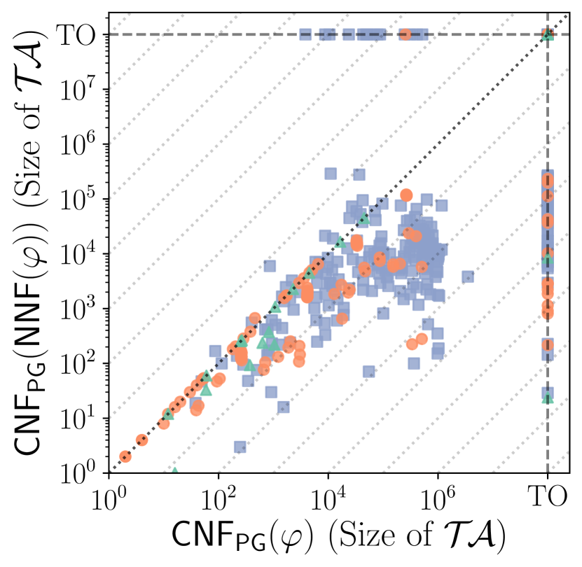
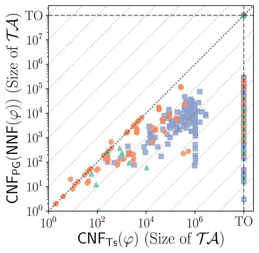
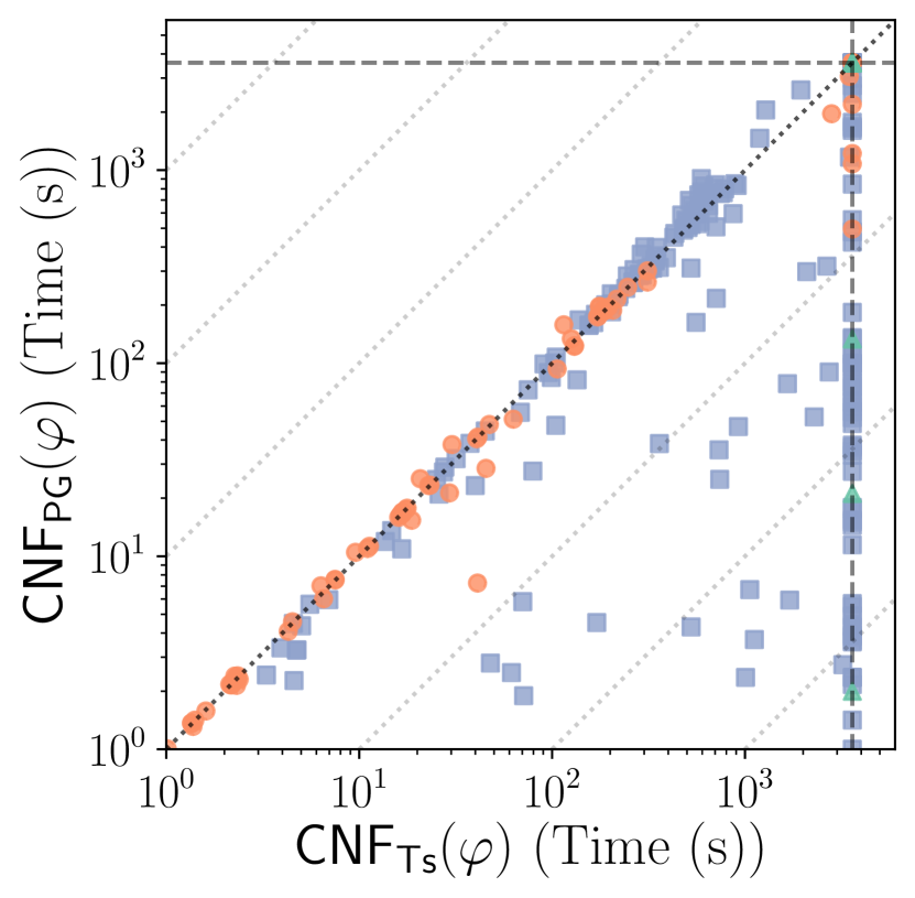
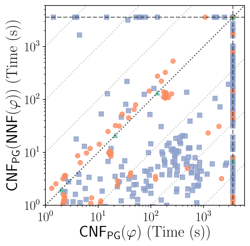
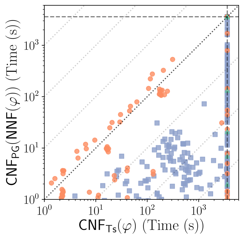
(a) Results for disjoint enumeration.

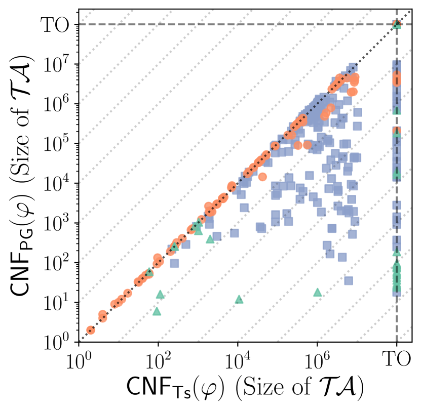
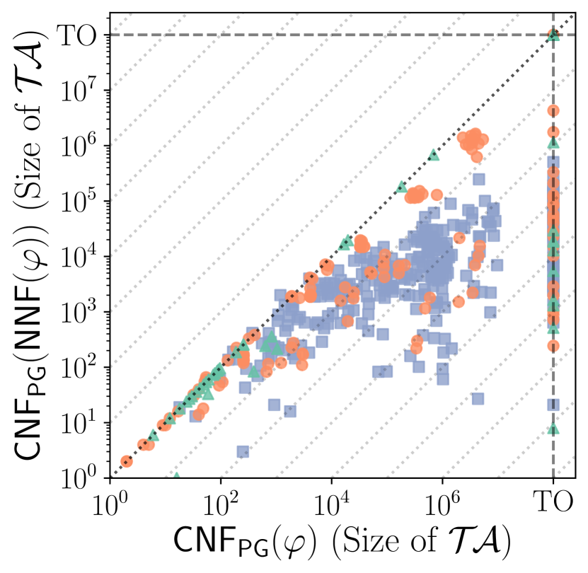
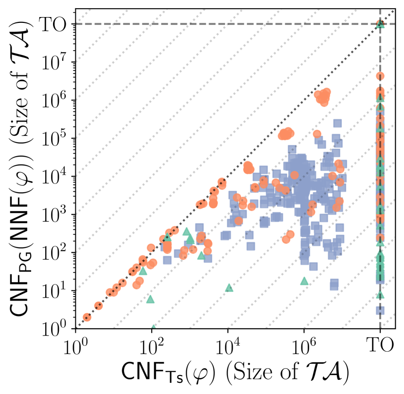
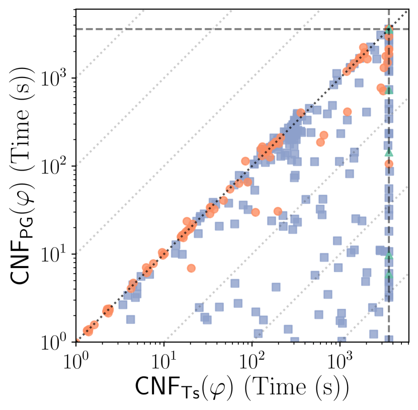
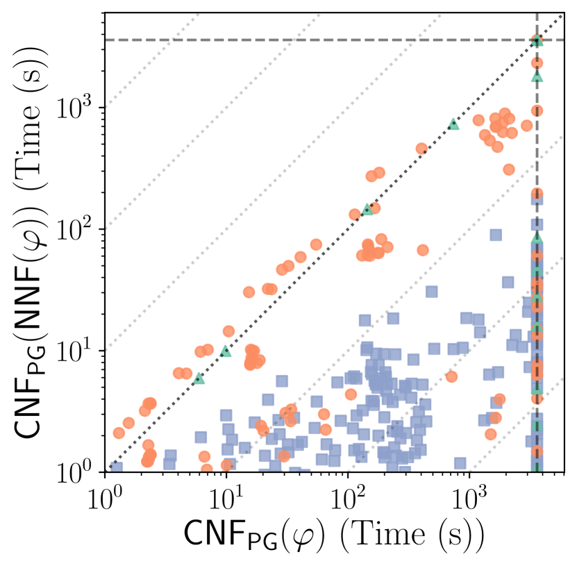
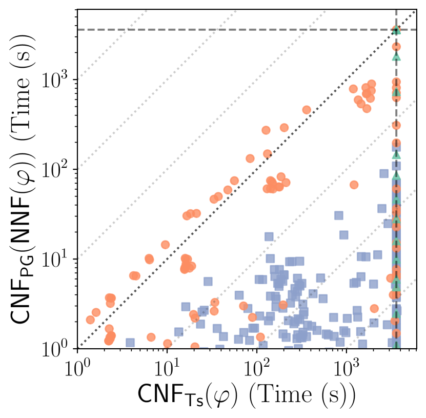
(b) Results for non-disjoint enumeration.

Figure 1: Set of scatter plots comparing the different CNF-izations on all the Boolean benchmarks. The first and second rows compare them in terms of size of $\mathcal{T}\mathcal{A}$ and execution time, respectively. The points on the dashed lines represent the timeouts. All the axes are on a logarithmic scale.

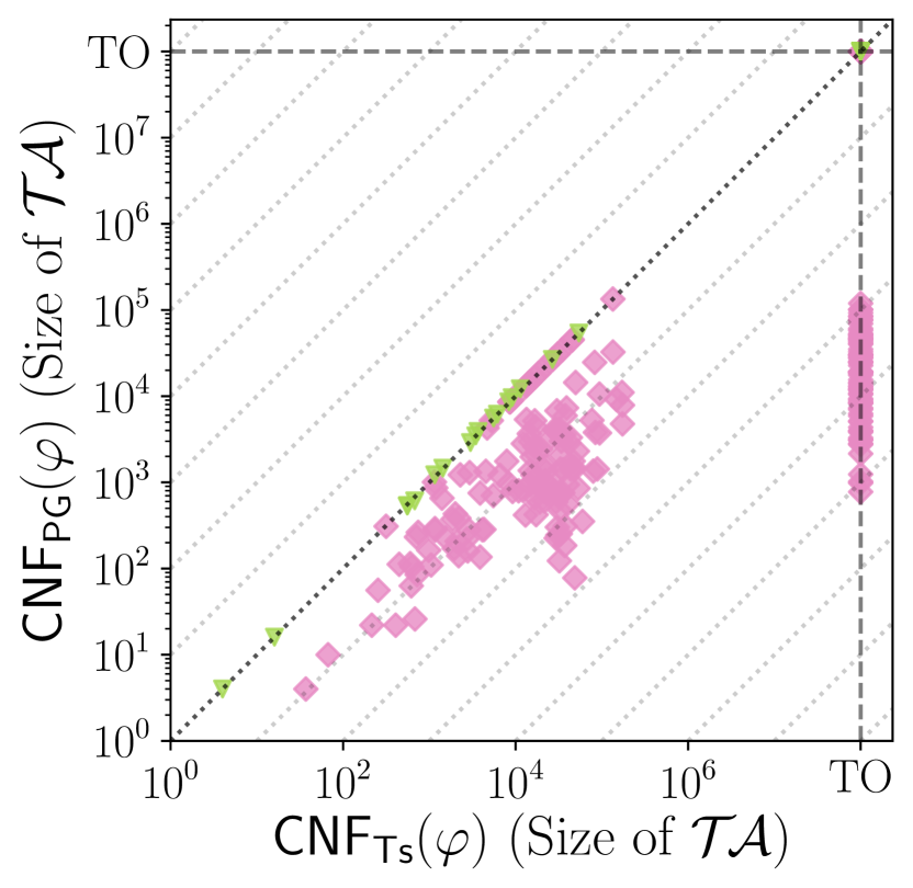
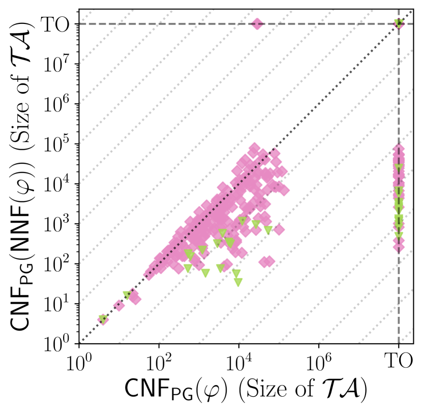
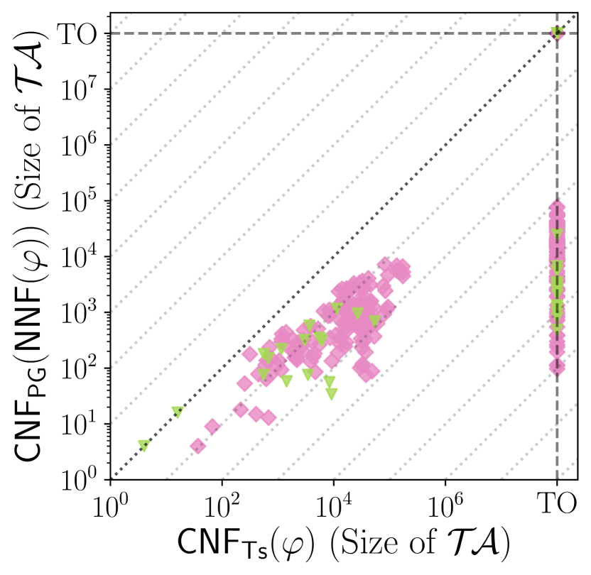
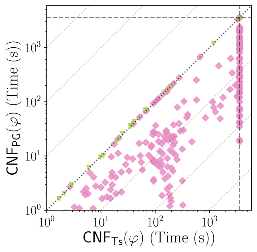
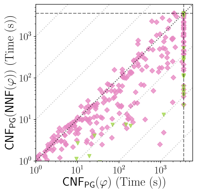
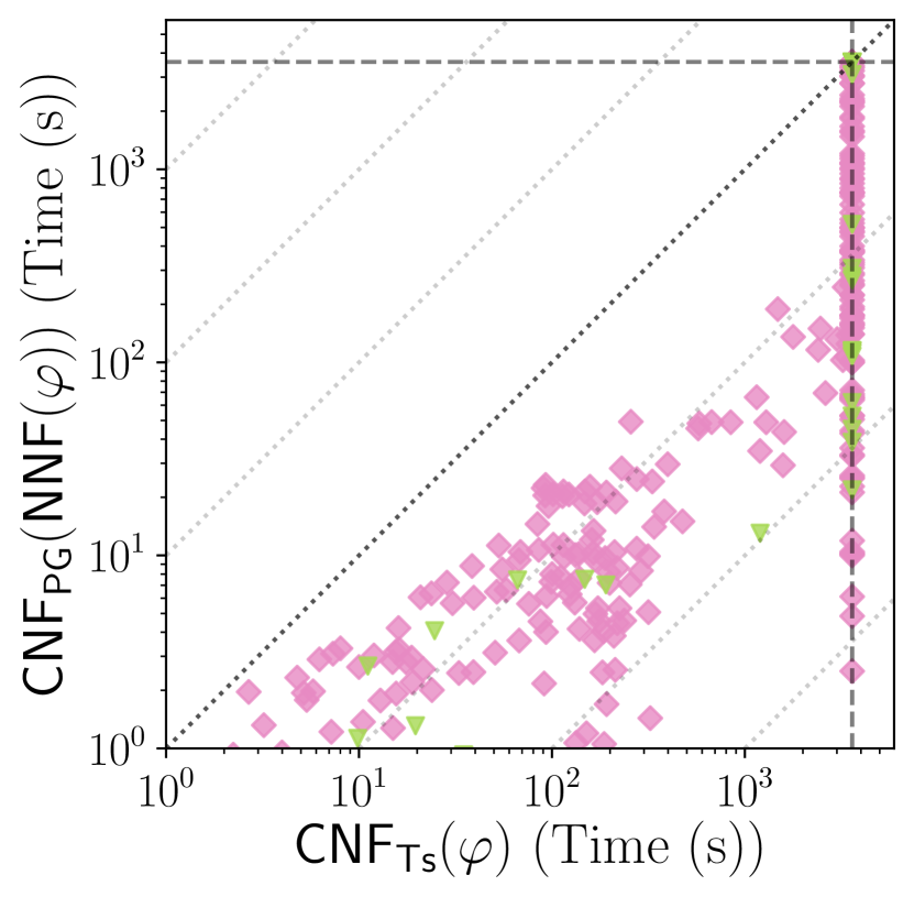
(a) Results for disjoint enumeration.

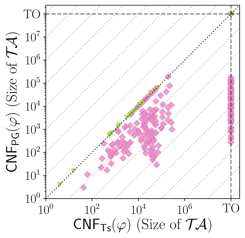
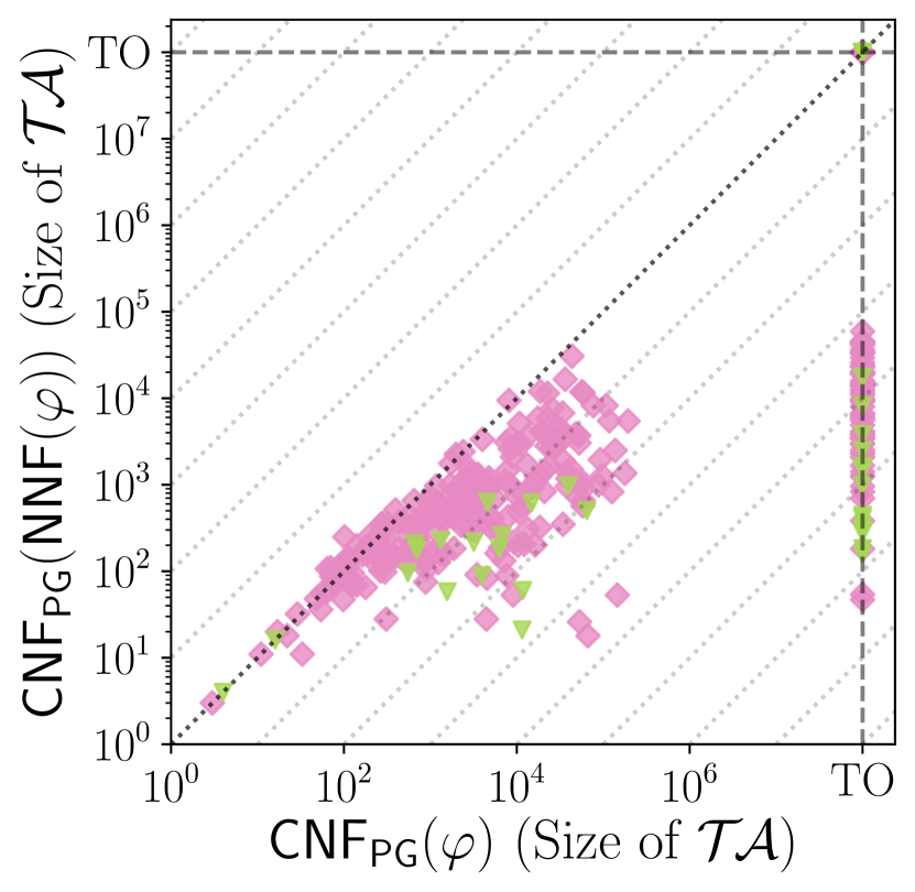
(b) Results for non-disjoint enumeration.

Figure 2: Set of scatter plots comparing the different CNF-izations all the $\text{SMT}(\mathcal{LRA})$ benchmarks. The first and second rows compare them in terms of size of $\mathcal{T}\mathcal{A}$ and execution time, respectively. The points on the dashed lines represent the timeouts. All the axes are on a logarithmic scale.

Bench.	Instances	T.O. disjoint AllSAT			T.O. non-disjoint AllSAT
		$\mathsf{CNF_{Ts}}$	$\mathsf{CNF_{PG}}$	$\mathsf{NNF}$+$\mathsf{CNF_{PG}}$	$\mathsf{CNF_{Ts}}$	$\mathsf{CNF_{PG}}$	$\mathsf{NNF}$+$\mathsf{CNF_{PG}}$
Syn-Bool	300	151	84	20	88	48	0
ISCAS85	250	47	43	30	27	22	1
AIG	89	79	73	71	78	60	50

Figure 3: Number of timeouts for the plots in Figure 1.

Bench.	Instances	T.O. disjoint AllSMT			T.O. non-disjoint AllSMT
		$\mathsf{CNF_{Ts}}$	$\mathsf{CNF_{PG}}$	$\mathsf{NNF}$+$\mathsf{CNF_{PG}}$	$\mathsf{CNF_{Ts}}$	$\mathsf{CNF_{PG}}$	$\mathsf{NNF}$+$\mathsf{CNF_{PG}}$
Syn-LRA	300	155	88	48	152	74	7
WMI	40	23	23	9	23	23	9

Figure 4: Number of timeouts for the plots in Figure 2.

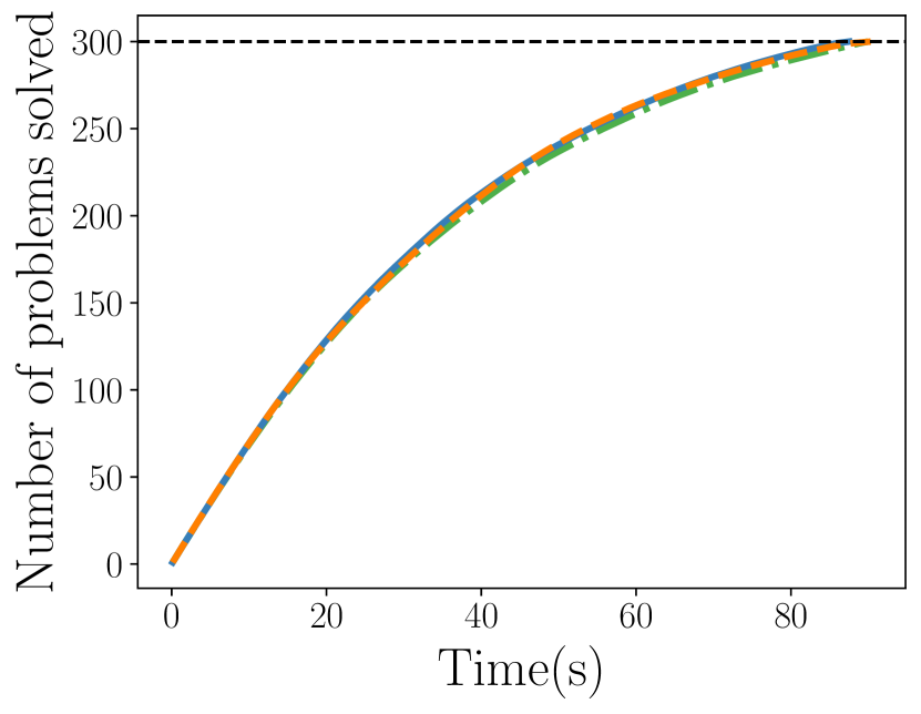
(a) Boolean synthetic

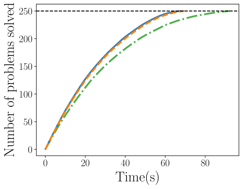
(b) ISCAS’85

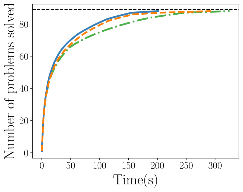
(c) AIG

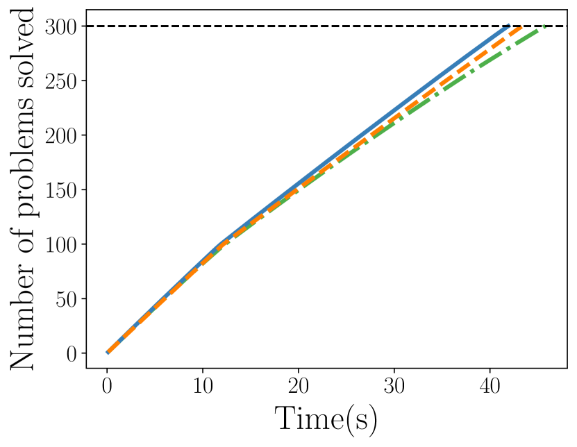
(d) $\text{SMT}(\mathcal{LRA})$ synthetic

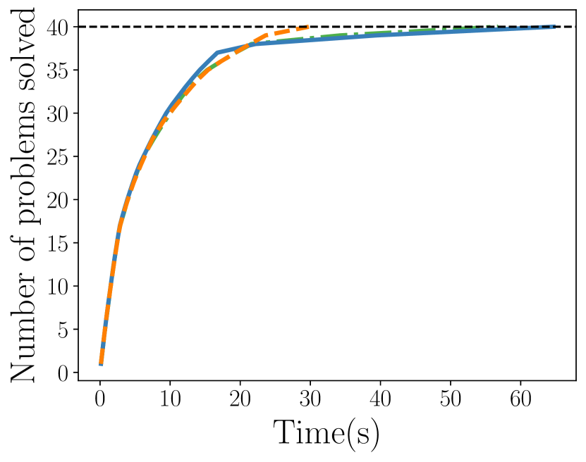
(e) WMI

Figure 5: CDF of the time taken for plain SAT and SMT solving using the different CNF transformations. The $y$-axis reports the instances for which the solver finished within the cumulative time on the $x$-axis.

6 Related work

Applications of AllSAT and AllSMT.

SAT and SMT enumeration has an important role in a variety of applications, ranging from artificial intelligence to formal verification. AllSAT and AllSMT, mainly in their disjoint version, play a foundational role in several frameworks for probabilistic reasoning, such as model counting in SMT (#SMT) (?) and Weighted Model Integration (WMI) (?, ?, ?, ?, ?). Specifically, #$\text{SMT}(\mathcal{LRA})$ (?, ?, ?) consists in summing up the volumes of the convex polytopes defined by each of the $\mathcal{LRA}$-satisfiable truth assignments propositionally satisfying a $\text{SMT}(\mathcal{LRA})$ formula, and has been employed for value estimation of probabilistic programs (?) and for quantitative program analysis (?). WMI can be seen as a generalization of #$\text{SMT}(\mathcal{LRA})$ that additionally considers a weight function $w$ that has to be integrated over each of such polytopes, and has been used to perform inference in hybrid probabilistic models such as Bayesian and Markov networks (?) and Density Estimation Trees (?). AllSAT has applications also in data mining, where the problem of frequent itemsets can be encoded into a propositional formula whose satisfying assignments are the frequent itemsets (?, ?). It has also been used in the context of software testing to generate a suite of test inputs that should match a given output (?), and in circuit design, to convert a formula from CNF to DNF (?, ?, ?), and for Static Timing Analysis to determine the inputs that can trigger a timing violation in a circuit (?). AllSAT and AllSMT have been applied also in network verification for checking network reachability and for analysing the correctness and consistency of network connectivity policies (?, ?, ?). Moreover, they have been used for computing the image and preimage of a given set of states in unbounded model checking (?, ?, ?), and they are also at the core of algorithms for computing predicate abstraction, a concept widely used in formal verification for automatically computing finite-state abstractions for systems with potentially infinite state space (?, ?, ?).

AllSAT.

Most of the works on AllSAT have focused on the enumeration of satisfying assignments for CNF formulas (e.g., ?, ?, ?, ?, ?, ?, ?), with several efforts in developing efficient and effective techniques for minimizing partial assignments (e.g., ?, ?, ?). The problem of minimizing truth assignments for Tseitin-encoded problems was addressed by ? (?). They propose to make iterative calls to a SAT solver imposing increasingly tighter cardinality constraints to obtain a minimal assignment. Whereas this approach can be used to find a single short truth assignment, it can be very expensive, and thus it is unsuitable for enumeration.

Other works have concentrated on the enumeration of satisfying assignments for combinatorial circuits, exploiting the structural information of the circuits to minimize the partial assignments over the input variables (e.g., ?, ?, ?, ?).

A problem closely-related to AllSAT is that of finding all the prime implicants of a formula (e.g., ?, ?, ?). AllSAT is a much simpler problem, and can be viewed as the problem of finding a not-necessarily-prime implicant cover for the formula.

Projected AllSAT.

Projected enumeration, i.e., enumeration of satisfying assignments over a set of relevant atoms, has been studied mainly for CNF formulas, e.g., by ? (?, ?, ?, ?). The ambiguity of the notion of “satisfiability by partial assignment” for non-CNF and existentially-quantified formulas has been raised by ? (?, ?), highlighting the difference between “evaluation to true”, which is simpler to check and typically used by SAT solvers, and “logical entailment”, which allows for producing shorter assignments. The approach based on dual reasoning by ? (?, ?), although able to detect logical entailment and thus to produce shorter partial assignments, is very inefficient even for small formulas.

AllSMT.

The literature on AllSMT is very limited, and AllSMT algorithms are highly based on AllSAT techniques and tools. E.g., MathSAT5 (?) implements an AllSMT functionality based on the procedure by ? (?). A similar procedure has been described and implemented by ? (?).

The role of CNF encodings.

Although most AllSAT solvers assume the formulas to be in CNF, little or no work has been done to investigate the impact of the different CNF encodings on their effectiveness and efficiency. The role of the CNF-ization has been widely studied for SAT solving (e.g., ?, ?, ?, ?) and in a recent work also for propositional model counting in the context of feature model analysis (?).

Dual-rail encoding.

The idea of using two different variables to represent the positive and negative occurrences of a sub-formula shares some similarities with the so-called dual-rail encoding (?, ?), which has been shown to be successful for prime implicant enumeration (?, ?), and recently also for SAT enumeration for combinatorial circuits (?).

Given a CNF formula, the dual-rail encoding maps each atom $A_{i}$ into a pair of dual-rail atoms $\langle{A_{i}^{\scalebox{0.5}[0.5]{$+$}}},{A_{i}^{\scalebox{0.5}[0.5]{$-$}}}\rangle$, so that $A_{i}$ and $\neg{}A_{i}$ are substituted with $A_{i}^{\scalebox{0.5}[0.5]{$+$}}$ and $A_{i}^{\scalebox{0.5}[0.5]{$-$}}$, respectively, and the clause $(\neg A_{i}^{\scalebox{0.5}[0.5]{$+$}}\vee\neg A_{i}^{\scalebox{0.5}[0.5]{$-$}})$ is conjoined with the formula. The resulting CNF formula is equisatisfiable to the original one, and every total assignment $\eta$ satisfying the dual-rail encoding corresponds to a partial assignment $\mu$ satisfying the original formula. Such $\mu$ can be obtained by assigning $\mu(A_{i})$ to $\top$ or $\bot$ if the pair $\langle{\eta(A_{i}^{\scalebox{0.5}[0.5]{$+$}})},{\eta(A_{i}^{\scalebox{0.5}[0.5]{$-$}})}\rangle$ is $\langle{\top},{\bot}\rangle$ or $\langle{\bot},{\top}\rangle$, respectively, while leaving it unassigned if $\langle{\eta(A_{i}^{\scalebox{0.5}[0.5]{$+$}})},{\eta(A_{i}^{\scalebox{0.5}[0.5]{$-$}})}\rangle=\langle{\bot},{\bot}\rangle$. Short partial assignments can be obtained by maximizing the number of pairs assigned to $\langle{\bot},{\bot}\rangle$, which can be done either exactly by solving a MaxSAT problem or approximately by assigning negative value first in decision branches (?).

Using the dual-rail encoding for enumeration, however, requires ad-hoc enumeration algorithms, since the solver must take into account the three-valued semantics of truth assignments over dual-rail atoms when enumerating the assignments (?). Our contribution, instead, focuses on CNF-ization approaches, which can be used in combination with any enumeration algorithm matching the properties described in §2.2. Also, comparing the $\mathsf{NNF}{}+\mathsf{CNF_{PG}}{}$ encoding with the dual-rail encoding, we observe that the former duplicates only the label atoms in $\mathbf{B}{}$, so that the number of introduced atoms is smaller than in the dual-rail encoding. Moreover, because of this, the clauses in the form $(\neg B_{i}^{\scalebox{0.5}[0.5]{$+$}}\vee\neg B_{i}^{\scalebox{0.5}[0.5]{$-$}})$ are not needed for correctness but only for efficiency, and can in principle be omitted. In the dual-rail encoding, instead, their presence is essential to prevent the illegal assignment $\eta(B_{i}^{\scalebox{0.5}[0.5]{$+$}})=\eta(B_{i}^{\scalebox{0.5}[0.5]{$-$}})=\top$.

7 Conclusions

We have presented a theoretical and empirical analysis of the impact of different CNF-ization approaches on SAT and SMT enumeration, both disjoint and non-disjoint. We have shown how the most popular transformations conceived for SAT and SMT solving, namely the Tseitin and the Plaisted and Greenbaum CNF-izations, prevent the solver from producing short partial assignments, thus seriously affecting the effectiveness of the enumeration. To overcome this limitation, we have proposed to preprocess the formula by converting it into NNF before applying the Plaisted and Greenbaum transformation. We have shown, both theoretically and empirically, that the latter approach can fully overcome the problem and can drastically reduce both the number of partial assignments and the execution time.

A Proofs

A.1 Proof for 1 in Section 2.1

(a) Case $\varphi\stackrel{{\scriptstyle\text{\scalebox{0.7}{def}}}}{{=}}\varphi_{1}\wedge\varphi_{2}$

(b) Case $\varphi\stackrel{{\scriptstyle\text{\scalebox{0.7}{def}}}}{{=}}\varphi_{1}\leftrightarrow\varphi_{2}$

Figure 6: 2-root DAGs for the pair $\langle{\mathsf{NNF}(\varphi)},\mathsf{NNF}(\neg\varphi)\rangle$ for $\varphi\stackrel{{\scriptstyle\text{\scalebox{0.7}{def}}}}{{=}}\varphi_{1}\wedge\varphi_{2}$ and $\varphi\stackrel{{\scriptstyle\text{\scalebox{0.7}{def}}}}{{=}}\varphi_{1}\leftrightarrow\varphi_{2}$ (those for $\varphi_{1}\vee\varphi_{2}$ and $\varphi_{1}\rightarrow\varphi_{2}$ are similar to that of $\varphi_{1}\wedge\varphi_{2}$).

Proof.

The NNF DAG that represents $\mathsf{NNF}(\varphi)$ is a sub-graph of the 2-root DAG for the pair $\langle{\mathsf{NNF}(\varphi)},\mathsf{NNF}(\neg\varphi)\rangle$ We prove that the latter grows linearly in size w.r.t. $\varphi$ by reasoning inductively on the structure of $\varphi$. (The size of a DAG “$\dots$” is denoted with “$|\dots|$”.)

if $\varphi$ is an atom:

$\mathsf{NNF}(\varphi)=\varphi$ and $\mathsf{NNF}(\neg\varphi)=\neg\varphi$, so that $|\langle\mathsf{NNF}(\varphi),\mathsf{NNF}(\neg\varphi)\rangle|=2$.

if $\varphi\stackrel{{\scriptstyle\text{\scalebox{0.7}{def}}}}{{=}}\neg\varphi_{1}$:

we assume by induction that we have computed $\langle{\mathsf{NNF}(\varphi_{1}),\mathsf{NNF}(\neg\varphi_{1})}\rangle$. Then $\langle{\mathsf{NNF}(\varphi),\mathsf{NNF}(\neg\varphi)}\rangle=\langle{\mathsf{NNF}(\neg\varphi_{1}),\mathsf{NNF}(\varphi_{1})}\rangle$ (i.e., we just invert the order of the pair), so that $|\langle{\mathsf{NNF}(\varphi),\mathsf{NNF}(\neg\varphi)}\rangle|=|\langle{\mathsf{NNF}(\neg\varphi_{1}),\mathsf{NNF}(\varphi_{1})}\rangle|=|\langle{\mathsf{NNF}(\varphi_{1}),\mathsf{NNF}(\neg\varphi_{1})}\rangle|$.

if $\varphi\stackrel{{\scriptstyle\text{\scalebox{0.7}{def}}}}{{=}}(\varphi_{1}\bowtie\varphi_{2})$ s.t. $\bowtie\ \in\{{\wedge,\leftrightarrow}\}$:

we assume by induction that we have computed $\langle{\mathsf{NNF}(\varphi_{1}),\mathsf{NNF}(\neg\varphi_{1})}\rangle$ and $\langle{\mathsf{NNF}(\varphi_{2}),\mathsf{NNF}(\neg\varphi_{2})}\rangle$. (See Figure 6). Then we show that

$$|\langle\mathsf{NNF}(\varphi),\mathsf{NNF}(\neg\varphi)\rangle|\leq 18+|\langle\mathsf{NNF}(\varphi_{1}),\mathsf{NNF}(\neg\varphi_{1})\rangle|+|\langle\mathsf{NNF}(\varphi_{2}),\mathsf{NNF}(\neg\varphi_{2})\rangle|:$$ (13)

if $\bowtie$ is $\wedge$:

the DAGs for $\mathsf{NNF}(\varphi)$ and $\mathsf{NNF}(\neg\varphi)$ add 2 “$\wedge/\vee$” nodes and $2+2$ arcs:
$\begin{aligned} \quad\mathsf{NNF}(\phantom{\neg}\phantom{(}\varphi_{1}\wedge\varphi_{2}\phantom{)})\stackrel{{\scriptstyle\text{\scalebox{0.7}{def}}}}{{=}}\mathsf{NNF}(\phantom{\neg}\varphi_{1})\wedge\mathsf{NNF}(\phantom{\neg}\varphi_{2});\\ \quad\mathsf{NNF}(\neg(\varphi_{1}\wedge\varphi_{2}))\stackrel{{\scriptstyle\text{\scalebox{0.7}{def}}}}{{=}}\mathsf{NNF}(\neg\varphi_{1})\vee\mathsf{NNF}(\neg\varphi_{2}).\end{aligned}$
Thus, $|\langle\mathsf{NNF}(\varphi),\mathsf{NNF}(\neg\varphi)\rangle|=6+|\langle\mathsf{NNF}(\varphi_{1}),\mathsf{NNF}(\neg\varphi_{1})\rangle|+|\langle\mathsf{NNF}(\varphi_{2}),\mathsf{NNF}(\neg\varphi_{2})\rangle|$.

if $\bowtie$ is $\leftrightarrow$:

the DAGs for $\mathsf{NNF}(\varphi)$ and $\mathsf{NNF}(\neg\varphi)$ share the sub-DAGs for $\mathsf{NNF}(\varphi_{1})$, $\mathsf{NNF}(\neg\varphi_{1})$, $\mathsf{NNF}(\varphi_{2})$, $\mathsf{NNF}(\neg\varphi_{2})$, adding 3+3 “$\wedge$”/“$\vee$” nodes and $6+6$ arcs:
$\begin{aligned} \quad\mathsf{NNF}(\phantom{\neg}\phantom{(}\varphi_{1}\leftrightarrow\varphi_{2}\phantom{)})\stackrel{{\scriptstyle\text{\scalebox{0.7}{def}}}}{{=}}(\mathsf{NNF}(\neg\varphi_{1})\vee\mathsf{NNF}(\phantom{\neg}\varphi_{2}))\wedge(\mathsf{NNF}(\phantom{\neg}\varphi_{1})\vee\mathsf{NNF}(\neg\varphi_{2}));\\ \quad\mathsf{NNF}(\neg(\varphi_{1}\leftrightarrow\varphi_{2}))\stackrel{{\scriptstyle\text{\scalebox{0.7}{def}}}}{{=}}(\mathsf{NNF}(\phantom{\neg}\varphi_{1})\vee\mathsf{NNF}(\phantom{\neg}\varphi_{2}))\wedge(\mathsf{NNF}(\neg\varphi_{1})\vee\mathsf{NNF}(\neg\varphi_{2})).\end{aligned}$
Thus, $|\langle\mathsf{NNF}(\varphi),\mathsf{NNF}(\neg\varphi)\rangle|=18+|\langle\mathsf{NNF}(\varphi_{1}),\mathsf{NNF}(\neg\varphi_{1})\rangle|+|\langle\mathsf{NNF}(\varphi_{2}),\mathsf{NNF}(\neg\varphi_{2})\rangle|$.

if $\varphi\stackrel{{\scriptstyle\text{\scalebox{0.7}{def}}}}{{=}}(\varphi_{1}\bowtie\varphi_{2})$ s.t. $\bowtie\ \in\{{\vee,\rightarrow}\}$:

these cases can be reduced to the previous cases, since $\mathsf{NNF}(\varphi_{1}\vee\varphi_{2})=\mathsf{NNF}(\neg(\neg\varphi_{1}\wedge\neg\varphi_{2}))$ and $\mathsf{NNF}(\varphi_{1}\rightarrow\varphi_{2})=\mathsf{NNF}(\neg(\varphi_{1}\wedge\neg\varphi_{2}))$.

Therefore, overall, from (13) we have that $|\langle\mathsf{NNF}(\varphi),\mathsf{NNF}(\neg\varphi)\rangle|$ is $O(|\varphi|)$. ∎

A.2 Proof for 2 in Section 2.1

$\begin{array}[]{||c||l|l|l|l|l|l|l|l|l||}\hline\cr\varphi_{1}|_{\mu}&\top&\top&\top&*&*&*&\bot&\bot&\bot\\ \varphi_{2}|_{\mu}&\top&*&\bot&\top&*&\bot&\top&*&\bot\\ \hline\cr\neg(\varphi_{1}|_{\mu})&\bot&\bot&\bot&*&*&*&\top&\top&\top\\ \varphi_{1}|_{\mu}\wedge\varphi_{2}|_{\mu}&\top&*&\bot&*&*&\bot&\bot&\bot&\bot\\ \varphi_{1}|_{\mu}\vee\varphi_{2}|_{\mu}&\top&\top&\top&\top&*&*&\top&*&\bot\\ \varphi_{1}|_{\mu}\rightarrow\varphi_{2}|_{\mu}&\top&*&\bot&\top&*&*&\top&\top&\top\\ \varphi_{1}|_{\mu}\leftrightarrow\varphi_{2}|_{\mu}&\top&*&\bot&*&*&*&\bot&*&\top\\ \hline\cr\end{array}$

Figure 7: Three-value-semantics of $\varphi|_{\mu}$ in terms of $\{{\top,\bot,*}\}$ (“true”, “false”, “unknown”).

In the following the symbol “$*$” denotes any formula which is not in $\{{\top,\bot}\}$. Following ? (?), we adopt a 3-value semantics for residuals $\varphi|_{\mu}\in\{{\top,\bot,*}\}$, so that “$\varphi|_{\mu}=*$” means “$\varphi|_{\mu}\not\in\{{\top,\bot}\}$” and “$\varphi_{1}|_{\mu}=\varphi_{2}|_{\mu}$” means that the two residuals $\varphi_{1}|_{\mu}$ and $\varphi_{2}|_{\mu}$ are either both $\top$, or both $\bot$, or neither is in $\{{\top,\bot}\}$. (Notice that, in the latter case, $\varphi_{1}|_{\mu}=\varphi_{2}|_{\mu}$ even when $\varphi_{1}|_{\mu}$ and $\varphi_{2}|_{\mu}$ are different formulas.) We extend this definition to tuples in an obvious way: $\langle{\varphi_{1}|_{\mu},\dots,\varphi_{n}|_{\mu}}\rangle=\langle{\psi_{1}|_{\mu},\dots,\psi_{n}|_{\mu}}\rangle$ iff $\varphi_{i}|_{\mu}=\psi_{i}|_{\mu}$ for each $i\in[1\dots n]$.

The 3-value semantics of the Boolean operators is reported for convenience in Figure 7. As a straightforward consequence of the above semantics, we have that:

$$(\neg\varphi)|_{\mu} = \neg(\varphi|_{\mu})\ \ \mbox{(hereafter simply ``$\neg\varphi|_{\mu}$'')}$$

$$(\varphi_{1}\bowtie\varphi_{2})|_{\mu} = \varphi_{1}|_{\mu}\bowtie\varphi_{2}|_{\mu}\ \ \mbox{for $\bowtie\ \in\{{\wedge,\vee,\rightarrow,\leftrightarrow}\}$}.$$

Also, the usual transformations apply: $\neg(\varphi_{1}\wedge\varphi_{2})|_{\mu}=\neg\varphi_{1}|_{\mu}\vee\neg\varphi_{2}|_{\mu}$, $\neg(\varphi_{1}\vee\varphi_{2})|_{\mu}=\neg\varphi_{1}|_{\mu}\wedge\neg\varphi_{2}|_{\mu}$, $(\varphi_{1}\leftrightarrow\varphi_{2})|_{\mu}=(\neg\varphi_{1}|_{\mu}\vee\varphi_{2}|_{\mu})\wedge(\varphi_{1}|_{\mu}\vee\neg\varphi_{2}|_{\mu})$ and $\neg(\varphi_{1}\leftrightarrow\varphi_{2})|_{\mu}=(\varphi_{1}|_{\mu}\vee\varphi_{2}|_{\mu})\wedge(\neg\varphi_{1}|_{\mu}\vee\neg\varphi_{2}|_{\mu})$. For convenience, sometimes we denote as $\bar{v}$ the complement of $v\in\{{\top,\bot,*}\}$, i.e. $\bar{v}\stackrel{{\scriptstyle\text{\scalebox{0.7}{def}}}}{{=}}\neg v$, so that $\bar{\top}=\bot,\bar{\bot}=\top,\bar{*}=*$.

We prove the following property, from which 2 in Section 2.1 follows directly.

Property 3.

Consider a formula $\varphi$, and let $\mathsf{NNF}(\varphi)$ be its NNF DAG. Consider a partial assignment $\mu$. Then:

$$\langle{\varphi|_{\mu}},{\neg\varphi|_{\mu}}\rangle=\langle{\mathsf{NNF}(\varphi)|_{\mu}},{\mathsf{NNF}(\neg\varphi)|_{\mu}}\rangle.$$ (14)

Proof.

As in Section A.1, we prove this fact by reasoning on the 2-root DAG for the pair $\langle\mathsf{NNF}(\varphi),\mathsf{NNF}(\neg\varphi)\rangle$. Specifically, we prove (14) by induction on the structure of $\varphi$.

if $\varphi$ is an atom:

then $\mathsf{NNF}(\varphi)=\varphi$ and $\mathsf{NNF}(\neg\varphi)=\neg\varphi$, so that $\varphi|_{\mu}=\mathsf{NNF}(\varphi)|_{\mu}$ and $\neg\varphi|_{\mu}=\mathsf{NNF}(\neg\varphi)|_{\mu}$.

if $\varphi\stackrel{{\scriptstyle\text{\scalebox{0.7}{def}}}}{{=}}\neg\varphi_{1}$:

we assume by induction that $\langle{\varphi_{1}|_{\mu}},{\neg\varphi_{1}|_{\mu}}\rangle=\langle{\mathsf{NNF}(\varphi_{1})|_{\mu}},{\mathsf{NNF}(\neg\varphi_{1})|_{\mu}}\rangle$. Let $v$ be s.t. $\langle{\varphi|_{\mu}},{\neg\varphi|_{\mu}}\rangle=\langle{v},{\bar{v}}\rangle$. Then:

$$\langle{\neg\varphi_{1}|_{\mu}},{\varphi_{1}|_{\mu}}\rangle=\langle{v},{\bar{v}}\rangle \Leftrightarrow$$

$$\langle{\varphi_{1}|_{\mu}},{\neg\varphi_{1}|_{\mu}}\rangle=\langle{\bar{v}},{v}\rangle \stackrel{{\scriptstyle\text{\scalebox{0.7}{ind}}}}{{\Leftrightarrow}}$$

$$\langle{\mathsf{NNF}(\varphi_{1})|_{\mu}},{\mathsf{NNF}(\neg\varphi_{1})|_{\mu}}\rangle=\langle{\bar{v}},{v}\rangle \Leftrightarrow$$

$$\langle{\mathsf{NNF}(\neg\varphi_{1})|_{\mu}},{\mathsf{NNF}(\varphi_{1})|_{\mu}}\rangle=\langle{v},{\bar{v}}\rangle$$

if $\varphi\stackrel{{\scriptstyle\text{\scalebox{0.7}{def}}}}{{=}}(\varphi_{1}\bowtie\varphi_{2})$:

s.t. $\bowtie~{}\in\{{\wedge,\leftrightarrow}\}$. We assume by induction that

$$\langle{\varphi_{1}|_{\mu}},{\neg\varphi_{1}|_{\mu}}\rangle=\langle{\mathsf{NNF}(\varphi_{1})|_{\mu}},{\mathsf{NNF}(\neg\varphi_{1})|_{\mu}}\rangle,$$

$$\langle{\varphi_{2}|_{\mu}},{\neg\varphi_{2}|_{\mu}}\rangle=\langle{\mathsf{NNF}(\varphi_{2})|_{\mu}},{\mathsf{NNF}(\neg\varphi_{2})|_{\mu}}\rangle.$$

Then,

if $\bowtie$ is $\wedge$:

$$\langle(\varphi_{1}\wedge\varphi_{2})|_{\mu},\neg(\varphi_{1}\wedge\varphi_{2})|_{\mu}\rangle=\langle\varphi_{1}|_{\mu}\wedge\varphi_{2}|_{\mu},\neg\varphi_{1}|_{\mu}\vee\neg\varphi_{2}|_{\mu}\rangle \stackrel{{\scriptstyle\text{\scalebox{0.7}{ind}}}}{{=}}$$

$$\langle\mathsf{NNF}(\varphi_{1})|_{\mu}\wedge\mathsf{NNF}(\varphi_{2})|_{\mu},\mathsf{NNF}(\neg\varphi_{1})|_{\mu}\vee\mathsf{NNF}(\neg\varphi_{2})|_{\mu}\rangle =$$

$$\langle(\mathsf{NNF}(\varphi_{1})\wedge\mathsf{NNF}(\varphi_{2}))|_{\mu},(\mathsf{NNF}(\neg\varphi_{1})\vee\mathsf{NNF}(\neg\varphi_{2}))|_{\mu}\rangle =$$

$$\langle\mathsf{NNF}(\varphi_{1}\wedge\varphi_{2})|_{\mu},\mathsf{NNF}(\neg(\varphi_{1}\wedge\varphi_{2}))|_{\mu}\rangle$$

if $\bowtie$ is $\leftrightarrow$:

$$\langle(\varphi_{1}\leftrightarrow\varphi_{2})|_{\mu},\neg(\varphi_{1}\leftrightarrow\varphi_{2})|_{\mu}\rangle =$$

$$\langle((\neg\varphi_{1}\vee\varphi_{2})\wedge(\varphi_{1}\vee\neg\varphi_{2}))|_{\mu},((\varphi_{1}\vee\varphi_{2})\wedge(\varphi_{1}\vee\varphi_{2}))|_{\mu}\rangle =$$

$$\langle(\neg\varphi_{1}|_{\mu}\vee\varphi_{2}|_{\mu})\wedge(\varphi_{1}|_{\mu}\vee\neg\varphi_{2}|_{\mu}),(\varphi_{1}|_{\mu}\vee\varphi_{2}|_{\mu})\wedge(\varphi_{1}|_{\mu}\vee\varphi_{2}|_{\mu})\rangle \stackrel{{\scriptstyle\text{\scalebox{0.7}{ind}}}}{{=}}$$

$$\langle(\mathsf{NNF}(\neg\varphi_{1})|_{\mu}\vee\mathsf{NNF}(\varphi_{2})|_{\mu})\wedge(\mathsf{NNF}(\varphi_{1})|_{\mu}\vee\mathsf{NNF}(\neg\varphi_{2})|_{\mu}),$$

$$(\mathsf{NNF}(\varphi_{1})|_{\mu}\vee\mathsf{NNF}(\varphi_{2})|_{\mu})\wedge(\mathsf{NNF}(\varphi_{1})|_{\mu}\vee\mathsf{NNF}(\varphi_{2})|_{\mu})\rangle =$$

$$\langle((\mathsf{NNF}(\neg\varphi_{1})\vee\mathsf{NNF}(\varphi_{2}))\wedge(\mathsf{NNF}(\varphi_{1})\vee\mathsf{NNF}(\neg\varphi_{2})))|_{\mu},$$

$$((\mathsf{NNF}(\varphi_{1})\vee\mathsf{NNF}(\varphi_{2}))\wedge(\mathsf{NNF}(\varphi_{1})\vee\mathsf{NNF}(\varphi_{2})))|_{\mu}\rangle =$$

$$\langle\mathsf{NNF}(\varphi_{1}\leftrightarrow\varphi_{2})|_{\mu},\mathsf{NNF}(\neg(\varphi_{1}\leftrightarrow\varphi_{2}))|_{\mu}\rangle$$ .

if $\varphi\stackrel{{\scriptstyle\text{\scalebox{0.7}{def}}}}{{=}}(\varphi_{1}\bowtie\varphi_{2})$:

s.t. $\bowtie~{}\in\{{\vee,\rightarrow}\}$. These cases can be reduced to the previous cases, since $\mathsf{NNF}(\varphi_{1}\vee\varphi_{2})=\mathsf{NNF}(\neg(\neg\varphi_{1}\wedge\neg\varphi_{2}))$ and $\mathsf{NNF}(\varphi_{1}\rightarrow\varphi_{2})=\mathsf{NNF}(\neg(\varphi_{1}\wedge\neg\varphi_{2}))$.

∎

Thus, $\langle{\varphi|_{\mu}},{\neg\varphi|_{\mu}}\rangle=\langle{\mathsf{NNF}(\varphi)|_{\mu}},{\mathsf{NNF}(\neg\varphi)|_{\mu}}\rangle$ so that $\varphi|_{\mu}=v$ iff $\mathsf{NNF}(\varphi)|_{\mu}=v$ for every $v\in\{{\top,\bot}\}$, so that 2 in Section 2.1 holds.

A.3 Proof for Theorem 1 in Section 4

Proof.

We first show how such a $\eta^{\mathbf{B}}$ can be built, then we prove that it satisfies $\mathsf{CNF_{PG}}(\mathsf{NNF}(\varphi))$. For every sub-formula $\varphi_{i}$ of $\varphi$, whose positive and negative occurrences in $\mathsf{CNF_{PG}}(\mathsf{NNF}(\varphi))$ are associated with the variables $B_{i}^{\scalebox{0.5}[0.5]{$+$}}$ and $B_{i}^{\scalebox{0.5}[0.5]{$-$}}$ respectively, do:

1. if $\varphi_{i}|_{\mu^{\boldsymbol{\alpha}}}=\top$, and hence $\mathsf{NNF}(\varphi_{i})|_{\mu^{\boldsymbol{\alpha}}}=\top$ and $\mathsf{NNF}(\neg\varphi_{i})|_{\mu^{\boldsymbol{\alpha}}}=\bot$ by 2, then set $\eta^{\mathbf{B}}(B_{i}^{\scalebox{0.5}[0.5]{$+$}})=\top$ and $\eta^{\mathbf{B}}(B_{i}^{\scalebox{0.5}[0.5]{$-$}})=\bot$;

2. if $\varphi_{i}|_{\mu^{\boldsymbol{\alpha}}}=\bot$, and hence $\mathsf{NNF}(\varphi_{i})|_{\mu^{\boldsymbol{\alpha}}}=\bot$ and $\mathsf{NNF}(\neg\varphi_{i})|_{\mu^{\boldsymbol{\alpha}}}=\top$ by 2, then set $\eta^{\mathbf{B}}(B_{i}^{\scalebox{0.5}[0.5]{$+$}})=\bot$ and $\eta^{\mathbf{B}}(B_{i}^{\scalebox{0.5}[0.5]{$-$}})=\top$;

3. otherwise if $\varphi_{i}|_{\mu^{\boldsymbol{\alpha}}}\notin\{{\top,\bot}\}$, then let $\eta^{\mathbf{B}}(B_{i}^{\scalebox{0.5}[0.5]{$+$}})=\eta^{\mathbf{B}}(B_{i}^{\scalebox{0.5}[0.5]{$-$}})=\bot$;

(If $\varphi_{i}$ occurs only positively or negatively, then we only assign $B_{i}^{\scalebox{0.5}[0.5]{$+$}}$ or $B_{i}^{\scalebox{0.5}[0.5]{$-$}}$ respectively.)
We prove that $\mu^{\boldsymbol{\alpha}}\cup\eta^{\mathbf{B}}\models_{p}\mathsf{CNF_{PG}}(\mathsf{NNF}(\varphi))$ by induction on the structure of $\mathsf{CNF_{PG}}(\mathsf{NNF}(\varphi))$. Consider a sub-formula $\varphi_{i}$ of $\varphi$. Then

1. $\mathsf{CNF_{PG}}(\mathsf{NNF}(\varphi))\stackrel{{\scriptstyle\text{\scalebox{0.7}{def}}}}{{=}}\mathsf{CNF_{PG}}(\overbrace{\mathsf{NNF}(\varphi)[\mathsf{NNF}(\varphi_{i})|B_{i}^{\scalebox{0.5}[0.5]{$+$}}]}^{(1)}\wedge\overbrace{\left(\neg B_{i}^{\scalebox{0.5}[0.5]{$+$}}\vee\mathsf{NNF}(\varphi_{i})\right)}^{(2)})$ if $\varphi_{i}$ occurs positively in $\varphi$;

2. $\mathsf{CNF_{PG}}(\mathsf{NNF}(\varphi))\stackrel{{\scriptstyle\text{\scalebox{0.7}{def}}}}{{=}}\mathsf{CNF_{PG}}(\overbrace{\mathsf{NNF}(\varphi)[\mathsf{NNF}(\neg\varphi_{i})|B_{i}^{\scalebox{0.5}[0.5]{$-$}}]}^{(3)}\wedge\overbrace{\left(\neg B_{i}^{\scalebox{0.5}[0.5]{$-$}}\vee\mathsf{NNF}(\neg\varphi_{i})\right)}^{(4)})$ if $\varphi_{i}$ occurs negatively in $\varphi$;

For each pair of cases we have:

1. 1. $\mu^{\boldsymbol{\alpha}}\cup\eta^{\mathbf{B}}\models_{p}(1)$ since we substitute $\top$ for $\top$; $\mu^{\boldsymbol{\alpha}}\cup\eta^{\mathbf{B}}\models_{p}(2)$ since $\mu^{\boldsymbol{\alpha}}\models_{p}\mathsf{NNF}(\varphi_{i})$;

   2. $\mu^{\boldsymbol{\alpha}}\cup\eta^{\mathbf{B}}\models_{p}(3)$ since we substitute $\bot$ for $\bot$; $\mu^{\boldsymbol{\alpha}}\cup\eta^{\mathbf{B}}\models_{p}(4)$ since $\mu^{\boldsymbol{\alpha}}\models_{p}\neg B_{i}^{\scalebox{0.5}[0.5]{$-$}}$;

2. 1. $\mu^{\boldsymbol{\alpha}}\cup\eta^{\mathbf{B}}\models_{p}(1)$ since we substitute $\bot$ for $\bot$; $\mu^{\boldsymbol{\alpha}}\cup\eta^{\mathbf{B}}\models_{p}(2)$ since $\mu^{\boldsymbol{\alpha}}\models_{p}\neg B_{i}^{\scalebox{0.5}[0.5]{$+$}}$;

   2. $\mu^{\boldsymbol{\alpha}}\cup\eta^{\mathbf{B}}\models_{p}(3)$ since we substitute $\top$ for $\top$; $\mu^{\boldsymbol{\alpha}}\cup\eta^{\mathbf{B}}\models_{p}(4)$ since $\mu^{\boldsymbol{\alpha}}\models_{p}\mathsf{NNF}(\neg\varphi_{i})$;

3. 1. $\mu^{\boldsymbol{\alpha}}\cup\eta^{\mathbf{B}}\models_{p}(1)$ since we substitute $\bot$ for $*$; $\mu^{\boldsymbol{\alpha}}\cup\eta^{\mathbf{B}}\models_{p}(2)$ since $\mu^{\boldsymbol{\alpha}}\models_{p}\neg B_{i}^{\scalebox{0.5}[0.5]{$+$}}$;

   2. $\mu^{\boldsymbol{\alpha}}\cup\eta^{\mathbf{B}}\models_{p}(3)$ since we substitute $\bot$ for $*$; $\mu^{\boldsymbol{\alpha}}\cup\eta^{\mathbf{B}}\models_{p}(4)$ since $\mu^{\boldsymbol{\alpha}}\models_{p}\neg B_{i}^{\scalebox{0.5}[0.5]{$-$}}$;

Therefore, $\mu^{\boldsymbol{\alpha}}\cup\eta^{\mathbf{B}}\models_{p}\mathsf{CNF_{PG}}(\mathsf{NNF}(\varphi))$. ∎

B An analysis of candidate solvers

In Table 1 we report an analysis of the features of every candidate AllSAT and AllSMT solver, as discussed in §5.1.

		Required features					Options
	Solver	Available	CNF input	Projected	Partial	Minimal	Disjoint	Non-disjoint	Notes
AllSAT	RELSAT	✓	✓	✗	✗	✗	✓	✗
	Grumberg	✗	✓	✓	✓	✓	✓	✓	Ex-post minimization
	SOLALL	?	✓	✓	✓	✗	✓	✗	Result stored in (O)BDD
	Jin	✗	✗	✗	✓	✓	✗	✓	AIG input
	clasp	✓	✓	✓	✗	✗	✓	✗	ASP solver
	PicoSAT	✓	✓	✗	✗	✗	✓	✗
	Yu	?	✓	✗	✓	✓	✓	✓
	BC	✓	✓	✗	✓	✓	✓	✓
	NBC	✓	✓	✗	✗	✗	✓	✗
	BDD	✓	✓	✗	✓	✗	✗	✓	Result stored in (O)BDD
	depbdd	✗	✓	✓	✓	✗	✓	✗	Result stored in (O)BDD
	Dualiza	✓	✓	✓	✓	✗	✓	✓	Dual-reasoning-based
	BASolver	✗	✓	✗	✓	✓	✗	✓
	AllSATCC	✗	✓	✗	✓	✓	✓	✗
	HALL	✓	✗	✗	✓	✓	✓	✓	AIG input
	TabularAllSAT	✓	✓	✗	✓	✗	✓	✗
AllSMT
	MathSAT	✓	✓	✓	✓	✓	✓	✓
	aZ3	✓	✓	✓	✗	✗	✓	✗

Table 1: List of AllSAT and AllSMT solvers (rows) and supported features (columns).
(In the “Available” column, “✗” indicates that the authors confirmed to us the unavailability of their tool, whereas “?” indicates that they did not reply to our enquiry.)

C Details on experimental results

In this section, we report the scatter plots on individual benchmarks for the experiments presented in Section 5.3, Figures 1 and 2. In particular, Figures 9, LABEL:, 11, LABEL: and 13 show the results on the Boolean synthetic, ISCAS’85 and WMI benchmarks, respectively. Figures 15, LABEL: and 17 show the results of the AllSMT experiments on the synthetic and WMI benchmarks, respectively.

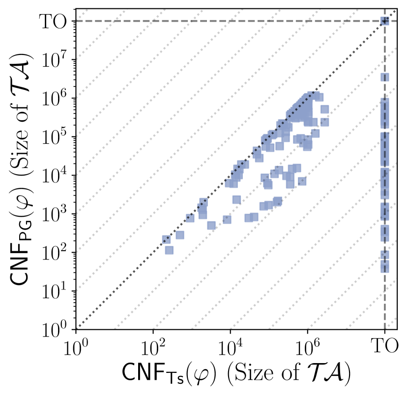
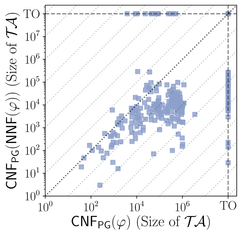
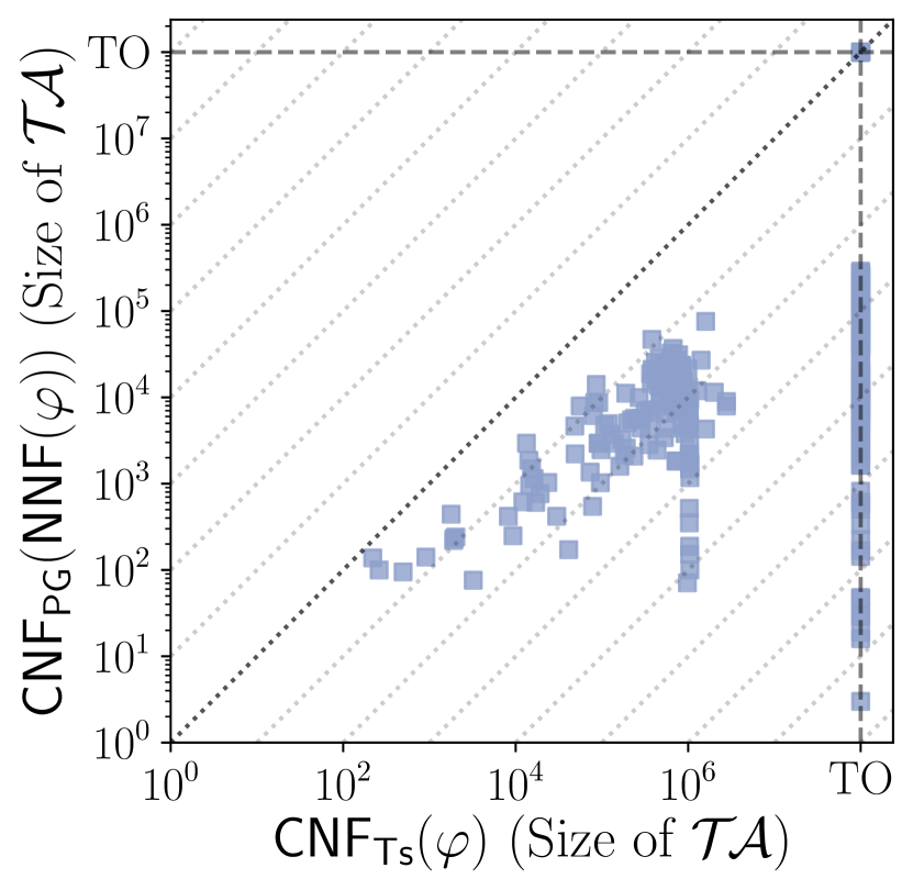
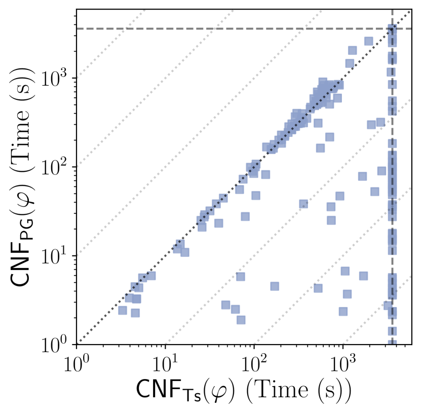
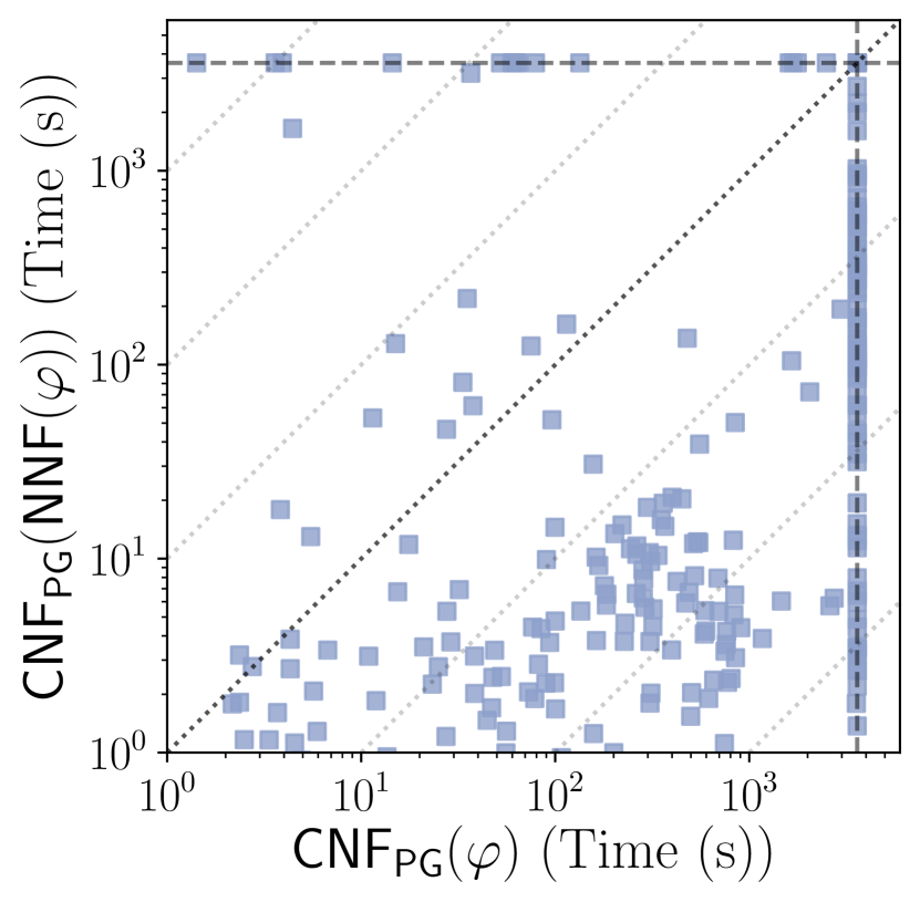
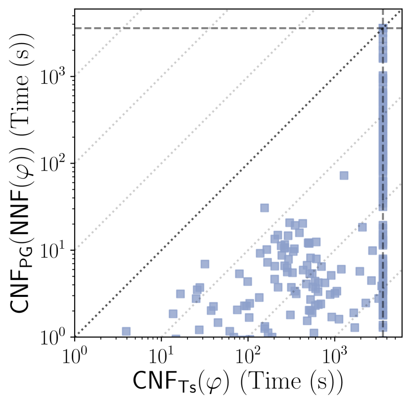
(a) Results for disjoint enumeration.

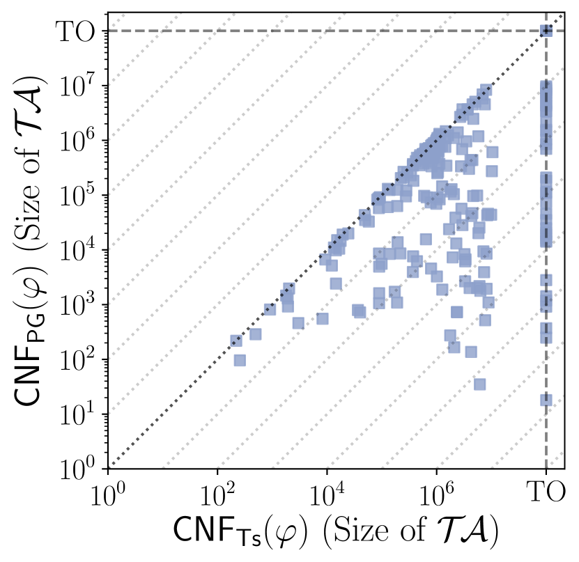
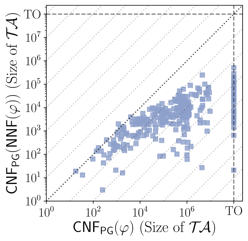
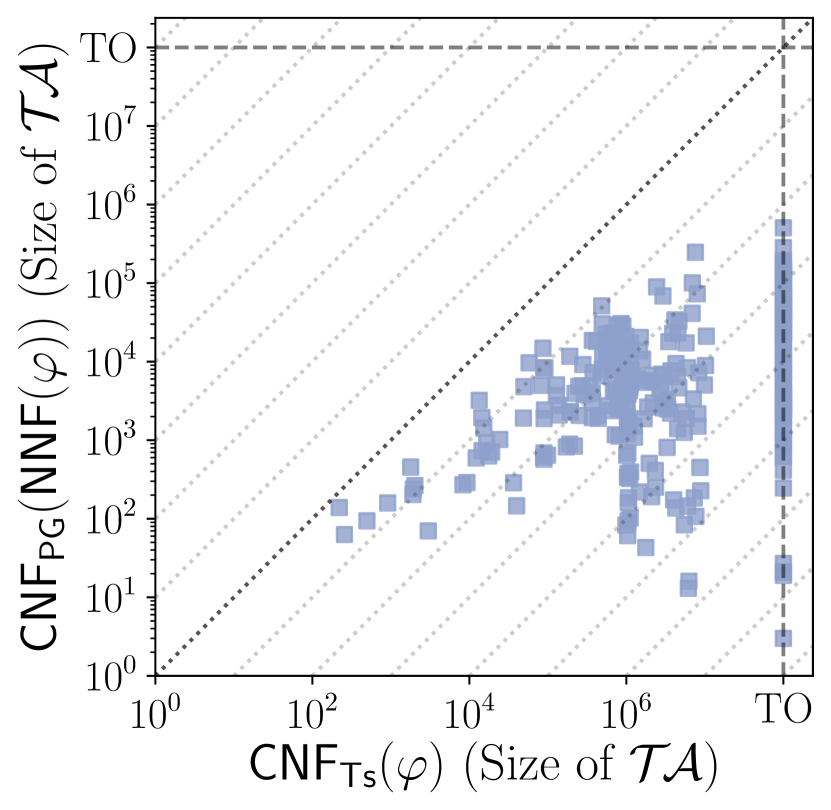
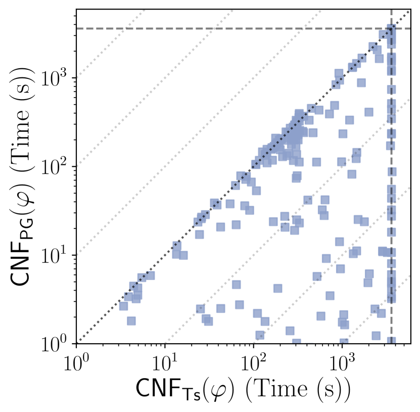
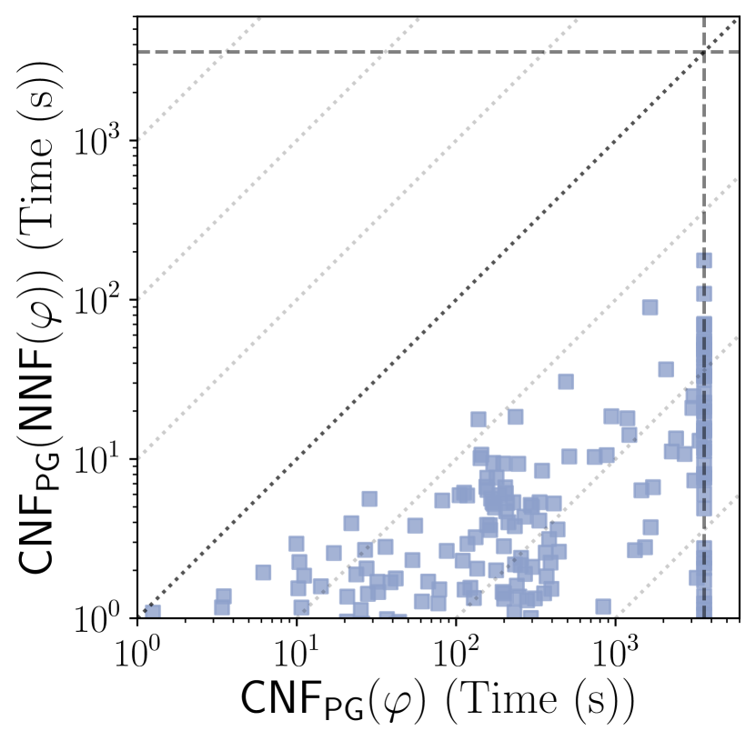
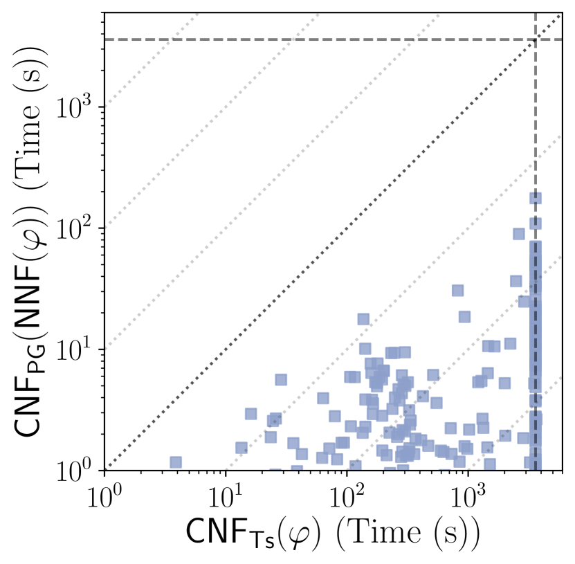
(b) Results for non-disjoint enumeration.

Figure 9: Set of scatter plots comparing the different CNF-izations on the Boolean synthetic benchmarks. The first and second rows compare them in terms of size of $\mathcal{T}\mathcal{A}$ and execution time, respectively. All the axes are on a logarithmic scale.

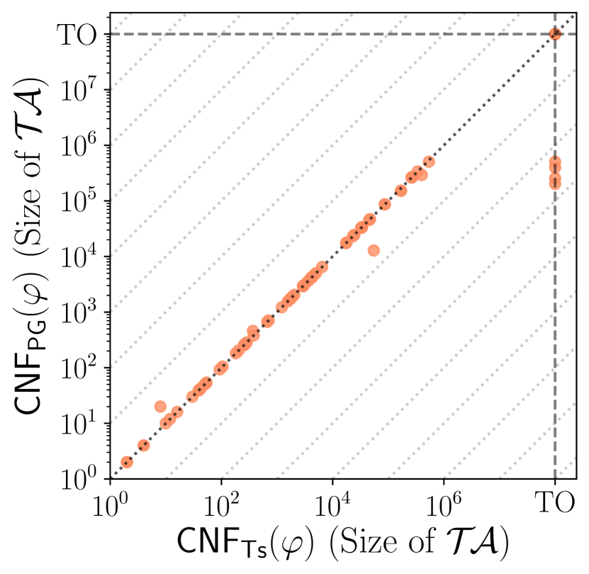
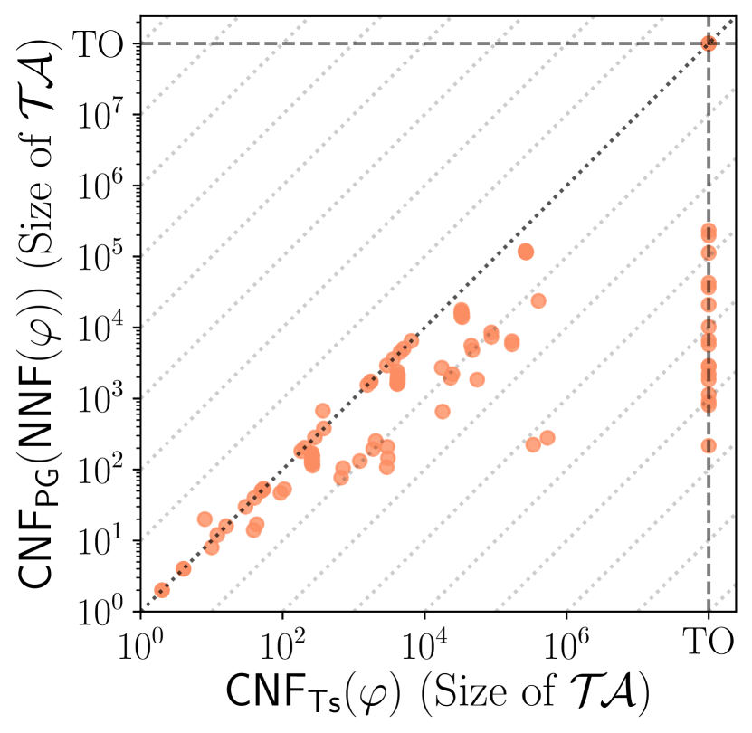
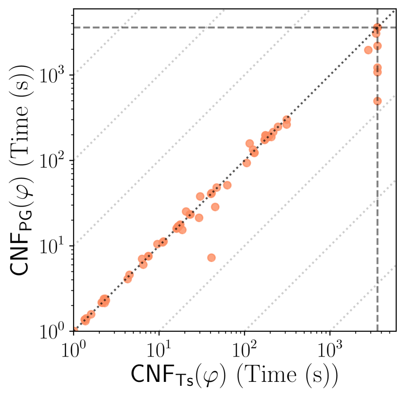
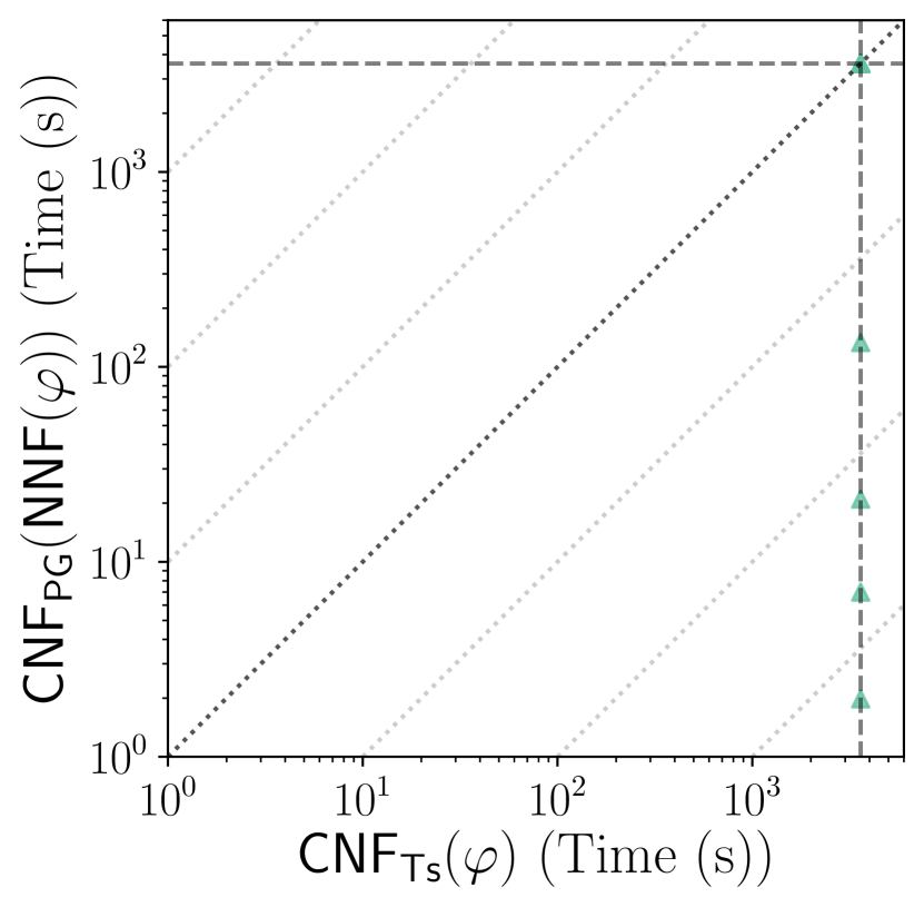
(a) Results for disjoint enumeration.

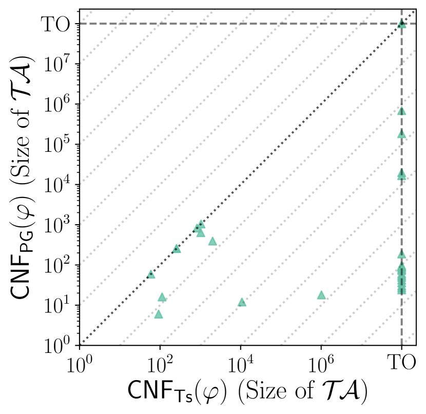
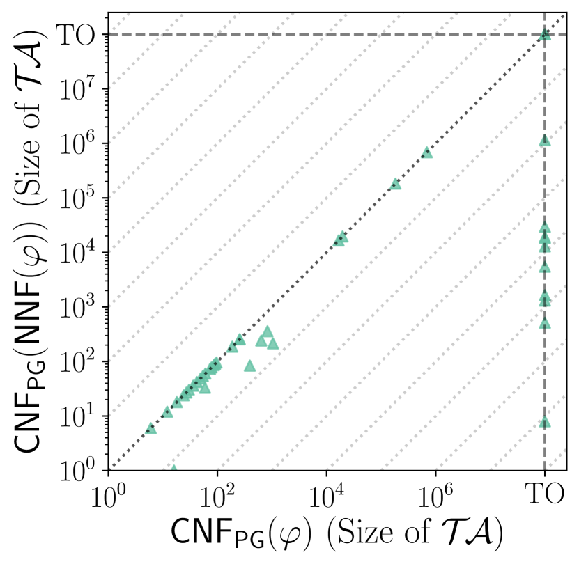
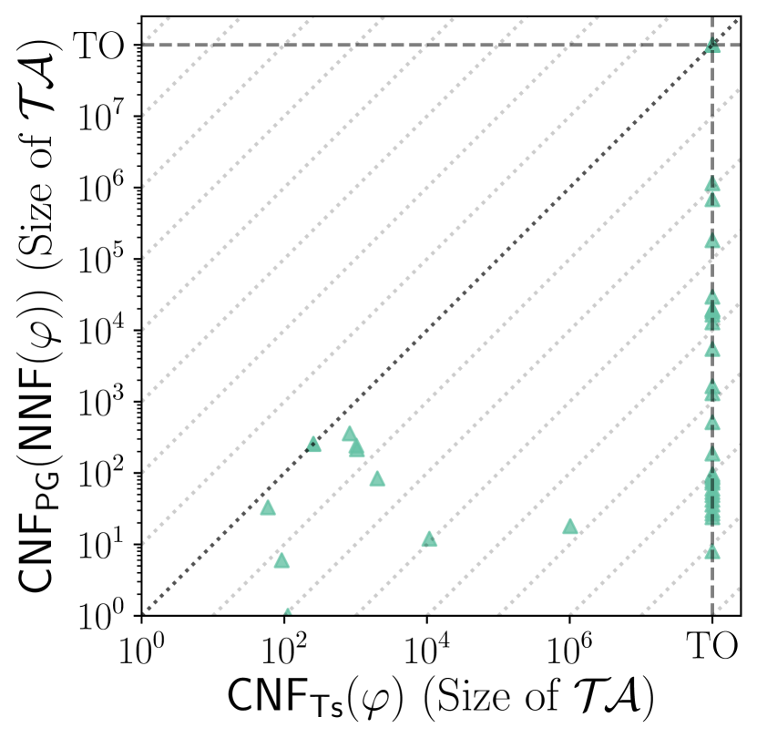
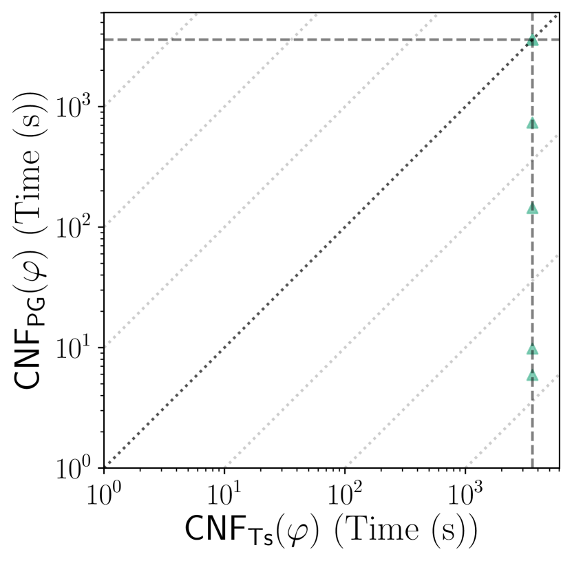
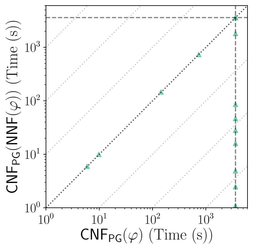
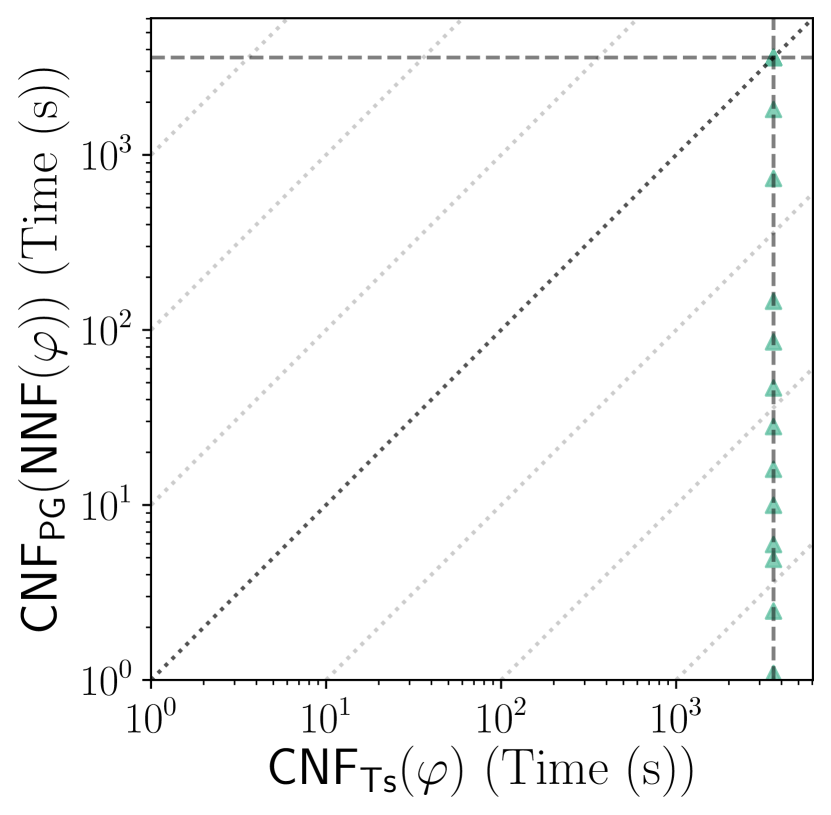
(b) Results for non-disjoint enumeration.

Figure 11: Set of scatter plots comparing the different CNF-izations on the ISCAS’85 benchmarks. The first and second rows compare them in terms of size of $\mathcal{T}\mathcal{A}$ and execution time, respectively. All the axes are on a logarithmic scale.

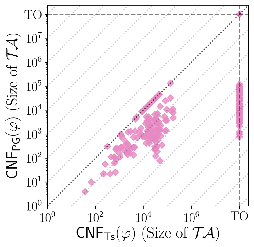
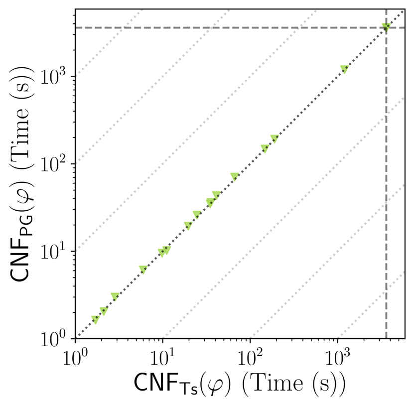
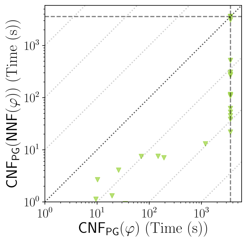
(a) Results for disjoint enumeration.

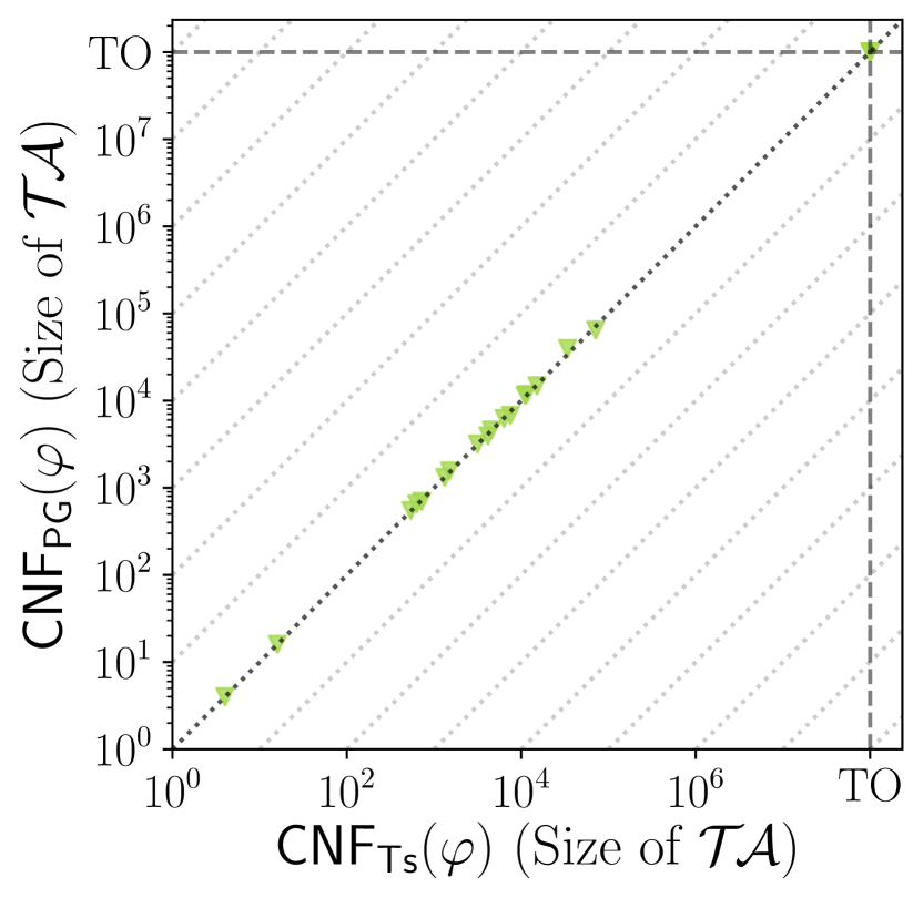
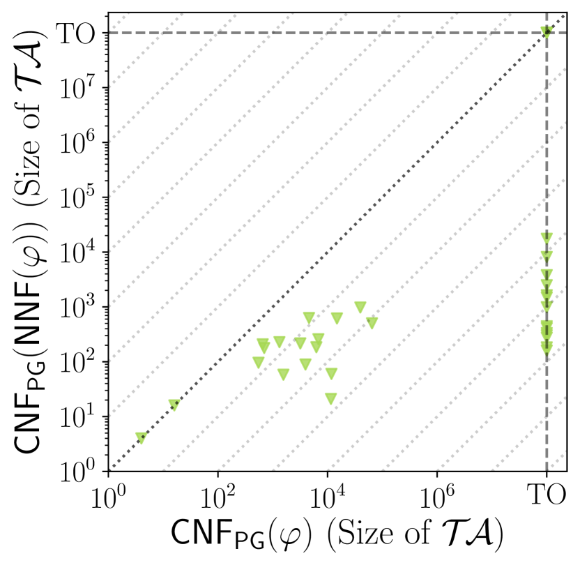
(b) Results for non-disjoint enumeration.

Figure 13: Set of scatter plots comparing the different CNF-izations on the AIG benchmarks. The first and second rows compare them in terms of size of $\mathcal{T}\mathcal{A}(\varphi)$ and execution time, respectively. All the axes are on a logarithmic scale.

(a) Results for disjoint enumeration.

(b) Results for non-disjoint enumeration.

Figure 15: Set of scatter plots comparing the different CNF-izations on the $\text{SMT}(\mathcal{LRA})$ synthetic benchmarks. The first and second rows compare them in terms of size of $\mathcal{T}\mathcal{A}$ and execution time, respectively. All the axes are on a logarithmic scale.

(a) Results for disjoint enumeration.

(b) Results for non-disjoint enumeration.

Figure 17: Set of scatter plots comparing the different CNF-izations on the WMI benchmarks. The first and second rows compare them in terms of size of $\mathcal{T}\mathcal{A}$ and execution time, respectively. All the axes are on a logarithmic scale.

References

• Amarù et al. Amarù, L., Gaillardon, P.-E., and De Micheli, G. (2015). The EPFL Combinational Benchmark Suite.  In Proceedings of the 24th International Workshop on Logic & Synthesis.
• Barrett et al. Barrett, C., Sebastiani, R., Seshia, S. A., and Tinelli, C. (2021). Satisfiability Modulo Theories.  In Biere, A., Heule, M., van Maaren, H., and Walsh, T. (Eds.), Handbook of Satisfiability (2 edition)., Vol. 336 of Frontiers in Artificial Intelligence and Applications, pp. 1267–1329. IOS Press.
• Bayardo and Schrag Bayardo, R. J.,  and Schrag, R. C. (1997). Using CSP look-back techniques to solve real-world SAT instances.  In Proceedings of the 14th AAAI Conference on Artificial Intelligence, AAAI’97, pp. 203–208. AAAI Press.
• Belle et al. Belle, V., Passerini, A., and den Broeck, G. V. (2015). Probabilistic Inference in Hybrid Domains by Weighted Model Integration.  In Proceedings of the 24th International Joint Conference on Artificial Intelligence, pp. 2770–2776. AAAI Press.
• Bernasconi et al. Bernasconi, A., Ciriani, V., Luccio, F., and Pagli, L. (2013). Compact DSOP and Partial DSOP Forms.  Theory of Computing Systems, 53(4), 583–608.
• Biere Biere, A. (2008). PicoSAT Essentials.  Journal on Satisfiability, Boolean Modeling and Computation, 4(2-4), 75–97.
• Björk Björk, M. (2009). Successful SAT Encoding Techniques.  Journal on Satisfiability, Boolean Modeling and Computation, 7(4), 189–201.
• Boudane et al. Boudane, A., Jabbour, S., Sais, L., and Salhi, Y. (2016). A SAT-based approach for mining association rules.  In Proceedings of the 25th International Joint Conference on Artificial Intelligence, IJCAI’16, pp. 2472–2478. AAAI Press.
• Boy de la Tour Boy de la Tour, T. (1992). An Optimality Result for Clause Form Translation.  Journal of Symbolic Computation, 14(4), 283–301.
• Brglez and Fujiwara Brglez, F.,  and Fujiwara, H. (1985). A Neutral Netlist of 10 Combinational Benchmark Circuits and a Target Translator in Fortran.  In Proceedings of IEEE International Symposium Circuits and Systems (ISCAS 85), pp. 677–692. IEEE Press.
• Bryant et al. Bryant, R. E., Beatty, D., Brace, K., Cho, K., and Sheffler, T. (1987). COSMOS: A compiled simulator for MOS circuits.  In Proceedings of the 24th ACM/IEEE Design Automation Conference, DAC ’87, pp. 9–16. Association for Computing Machinery.
• Chistikov et al. Chistikov, D., Dimitrova, R., and Majumdar, R. (2017). Approximate Counting in SMT and Value Estimation for Probabilistic Programs.  Acta Informatica, 54(8), 729–764.
• Cimatti et al. Cimatti, A., Griggio, A., Schaafsma, B. J., and Sebastiani, R. (2013). The MathSAT5 SMT Solver.  In Tools and Algorithms for the Construction and Analysis of Systems, Lecture Notes in Computer Science, pp. 93–107. Springer.
• Clarke et al. Clarke, E., Kroening, D., Sharygina, N., and Yorav, K. (2004). Predicate Abstraction of ANSI-C Programs Using SAT.  Formal Methods in System Design, 25(2), 105–127.
• Dlala et al. Dlala, I. O., Jabbour, S., Sais, L., and Yaghlane, B. B. (2016). A Comparative Study of SAT-Based Itemsets Mining.  In Bramer, M.,  and Petridis, M. (Eds.), Research and Development in Intelligent Systems XXXIII, pp. 37–52. Springer International Publishing.
• Fried et al. Fried, D., Nadel, A., and Shalmon, Y. (2023). AllSAT for Combinational Circuits.  In Mahajan, M.,  and Slivovsky, F. (Eds.), 26th International Conference on Theory and Applications of Satisfiability Testing, Vol. 271 of Leibniz International Proceedings in Informatics (LIPIcs), pp. 9:1–9:18. Schloss Dagstuhl – Leibniz-Zentrum für Informatik.
• Gario and Micheli Gario, M.,  and Micheli, A. (2015). PySMT: a solver-agnostic library for fast prototyping of SMT-based algorithms.  In SMT Workshop 2015.
• Ge et al. Ge, C., Ma, F., Zhang, P., and Zhang, J. (2018). Computing and estimating the volume of the solution space of SMT(LA) constraints.  Theoretical Computer Science, 743, 110–129.
• Gebser et al. Gebser, M., Kaufmann, B., Neumann, A., and Schaub, T. (2007). Conflict-Driven Answer Set Enumeration.  In Baral, C., Brewka, G., and Schlipf, J. (Eds.), Logic Programming and Nonmonotonic Reasoning, Vol. 4483, pp. 136–148. Springer Berlin Heidelberg.
• Grumberg et al. Grumberg, O., Schuster, A., and Yadgar, A. (2004). Memory Efficient All-Solutions SAT Solver and Its Application for Reachability Analysis.  In Hutchison, D., Kanade, T., Kittler, J., Kleinberg, J. M., Mattern, F., Mitchell, J. C., Naor, M., Nierstrasz, O., Pandu Rangan, C., Steffen, B., Sudan, M., Terzopoulos, D., Tygar, D., Vardi, M. Y., Weikum, G., Hu, A. J., and Martin, A. K. (Eds.), Formal Methods in Computer-Aided Design, Vol. 3312, pp. 275–289. Springer Berlin Heidelberg.
• Hansen et al. Hansen, M., Yalcin, H., and Hayes, J. (1999). Unveiling the ISCAS-85 benchmarks: a case study in reverse engineering.  IEEE Design & Test of Computers, 16(3), 72–80.
• Huang and Darwiche Huang, J.,  and Darwiche, A. (2005). Using DPLL for Efficient OBDD Construction.  In Hutchison, D., Kanade, T., Kittler, J., Kleinberg, J. M., Mattern, F., Mitchell, J. C., Naor, M., Nierstrasz, O., Pandu Rangan, C., Steffen, B., Sudan, M., Terzopoulos, D., Tygar, D., Vardi, M. Y., Weikum, G., Hoos, H. H., and Mitchell, D. G. (Eds.), Theory and Applications of Satisfiability Testing, Vol. 3542, pp. 157–172. Springer Berlin Heidelberg.
• Iser et al. Iser, M., Sinz, C., and Taghdiri, M. (2013). Minimizing Models for Tseitin-Encoded SAT Instances.  In 16th International Conference on Theory and Applications of Satisfiability Testing, Vol. 7962, pp. 224–232. Springer Berlin Heidelberg. Series Title: LNCS.
• Jabbour et al. Jabbour, S., Marques-Silva, J., Sais, L., and Salhi, Y. (2014). Enumerating Prime Implicants of Propositional Formulae in Conjunctive Normal Form.  In Fermé, E.,  and Leite, J. (Eds.), Logics in Artificial Intelligence, Lecture Notes in Computer Science, pp. 152–165. Springer International Publishing.
• Jackson and Sheridan Jackson, P.,  and Sheridan, D. (2005). Clause Form Conversions for Boolean Circuits.  In Hoos, H. H.,  and Mitchell, D. G. (Eds.), 7th International Conference on Theory and Applications of Satisfiability Testing, Lecture Notes in Computer Science, pp. 183–198, Berlin, Heidelberg. Springer.
• Jayaraman et al. Jayaraman, K., Bjørner, N., Outhred, G., and Kaufman, C. (2014). Automated analysis and debugging of network connectivity policies.  Tech. rep. MSR-TR-2014-102, Microsoft.
• Jin et al. Jin, H., Han, H., and Somenzi, F. (2005). Efficient Conflict Analysis for Finding All Satisfying Assignments of a Boolean Circuit.  In Hutchison, D., Kanade, T., Kittler, J., Kleinberg, J. M., Mattern, F., Mitchell, J. C., Naor, M., Nierstrasz, O., Pandu Rangan, C., Steffen, B., Sudan, M., Terzopoulos, D., Tygar, D., Vardi, M. Y., Weikum, G., Halbwachs, N., and Zuck, L. D. (Eds.), Tools and Algorithms for the Construction and Analysis of Systems, Vol. 3440, pp. 287–300. Springer Berlin Heidelberg.
• Jin and Somenzi Jin, H.,  and Somenzi, F. (2005). Prime Clauses for Fast Enumeration of Satisfying Assignments to Boolean Circuits.  In Proceedings of the 42nd Annual Design Automation Conference, pp. 750–753.
• Khurshid et al. Khurshid, S., Marinov, D., Shlyakhter, I., and Jackson, D. (2004). A Case for Efficient Solution Enumeration.  In Giunchiglia, E.,  and Tacchella, A. (Eds.), Theory and Applications of Satisfiability Testing, Lecture Notes in Computer Science, pp. 272–286. Springer.
• Kuiter et al. Kuiter, E., Krieter, S., Sundermann, C., Thüm, T., and Saake, G. (2022). Tseitin or not Tseitin? The Impact of CNF Transformations on Feature-Model Analyses.  In 37th IEEE/ACM Int. Conference on Automated Software Engineering, pp. 1–13. ACM.
• Lahiri et al. Lahiri, S. K., Bryant, R. E., and Cook, B. (2003). A Symbolic Approach to Predicate Abstraction.  In Hunt, W. A.,  and Somenzi, F. (Eds.), Computer Aided Verification, Lecture Notes in Computer Science, pp. 141–153. Springer.
• Lahiri et al. Lahiri, S. K., Nieuwenhuis, R., and Oliveras, A. (2006). SMT Techniques for Fast Predicate Abstraction.  In Computer Aided Verification, Vol. 4144 of Lecture Notes in Computer Science, pp. 424–437. Springer Berlin Heidelberg.
• Li et al. Li, B., Hsiao, M., and Sheng, S. (2004). A novel SAT all-solutions solver for efficient preimage computation.  In Automation and Test in Europe Conference and Exhibition Proceedings Design, Vol. 1, pp. 272–277.
• Liang et al. Liang, J., Ma, F., Zhou, J., and Yin, M. (2022). AllSATCC: Boosting AllSAT Solving with Efficient Component Analysis.  In Proceedings of the 31st International Joint Conference on Artificial Intelligence, pp. 1866–1872. International Joint Conferences on Artificial Intelligence Organization.
• Liu and Zhang Liu, S.,  and Zhang, J. (2011). Program Analysis: From Qualitative Analysis to Quantitative Analysis (NIER Track).  In 33rd International Conference on Software Engineering, pp. 956–959.
• Lopes et al. Lopes, N. P., Bjørner, N., Godefroid, P., Jayaraman, K., and Varghese, G. (2015). Checking Beliefs in Dynamic Networks.  In 12th USENIX Symposium on Networked Systems Design and Implementation, pp. 499–512.
• Lopes et al. Lopes, N. P., Bjørner, N., Godefroid, P., and Varghese, G. (2013). Network Verification in the Light of Program Verification.  MSR, Rep.
• Luo et al. Luo, W., Want, H., Zhong, H., Wei, O., Fang, B., and Song, X. (2021). An Efficient Two-phase Method for Prime Compilation of Non-clausal Boolean Formulae.  In 2021 IEEE/ACM International Conference On Computer Aided Design, pp. 1–9.
• Ma et al. Ma, F., Liu, S., and Zhang, J. (2009). Volume Computation for Boolean Combination of Linear Arithmetic Constraints.  In Schmidt, R. A. (Ed.), Automated Deduction, Lecture Notes in Computer Science, pp. 453–468. Springer.
• Masina et al. Masina, G., Spallitta, G., and Sebastiani, R. (2023). On CNF Conversion for Disjoint SAT Enumeration.  In Mahajan, M.,  and Slivovsky, F. (Eds.), 26th International Conference on Theory and Applications of Satisfiability Testing, Vol. 271 of Leibniz International Proceedings in Informatics (LIPIcs), pp. 15:1–15:16. Schloss Dagstuhl – Leibniz-Zentrum für Informatik.
• McMillan McMillan, K. L. (2002). Applying SAT Methods in Unbounded Symbolic Model Checking.  In Goos, G., Hartmanis, J., Van Leeuwen, J., Brinksma, E., and Larsen, K. G. (Eds.), Computer Aided Verification, Vol. 2404, pp. 250–264. Springer Berlin Heidelberg.
• Miltersen et al. Miltersen, P. B., Radhakrishnan, J., and Wegener, I. (2005). On converting CNF to DNF.  Theoretical Computer Science, 347(1-2), 325–335.
• Minato and De Micheli Minato, S.,  and De Micheli, G. (1998). Finding All Simple Disjunctive Decompositions Using Irredundant Sum-of-Products Forms.  In 1998 IEEE/ACM International Conference on Computer-Aided Design, pp. 111–117.
• Möhle and Biere Möhle, S.,  and Biere, A. (2018). Dualizing Projected Model Counting.  In IEEE 30th International Conference on Tools with Artificial Intelligence, pp. 702–709.
• Möhle et al. Möhle, S., Sebastiani, R., and Biere, A. (2020). Four Flavors of Entailment.  In 23rd International Conference on Theory and Applications of Satisfiability Testing, Lecture Notes in Computer Science, pp. 62–71. Springer.
• Möhle et al. Möhle, S., Sebastiani, R., and Biere, A. (2021). On Enumerating Short Projected Models.  arXiv:2110.12924 [cs].
• Morettin et al. Morettin, P., Passerini, A., and Sebastiani, R. (2017). Efficient Weighted Model Integration via SMT-Based Predicate Abstraction.  In Proceedings of the 26th International Joint Conference on Artificial Intelligence, pp. 720–728.
• Morettin et al. Morettin, P., Passerini, A., and Sebastiani, R. (2019). Advanced SMT techniques for Weighted Model Integration.  Artificial Intelligence, 275(C), 1–27.
• Morgado and Marques-Silva Morgado, A.,  and Marques-Silva, J. (2005). Good learning and implicit model enumeration.  In 17th IEEE International Conference on Tools with Artificial Intelligence, pp. 6 pp.–136.
• Palopoli et al. Palopoli, L., Pirri, F., and Pizzuti, C. (1999). Algorithms for selective enumeration of prime implicants.  Artificial Intelligence, 111(1-2), 41–72.
• Phan and Malacaria Phan, Q.-S.,  and Malacaria, P. (2015). All-Solution Satisfiability Modulo Theories: Applications, Algorithms and Benchmarks.  In 10th International Conference on Availability, Reliability and Security, pp. 100–109. IEEE.
• Plaisted and Greenbaum Plaisted, D. A.,  and Greenbaum, S. (1986). A Structure-preserving Clause Form Translation.  Journal of Symbolic Computation, 2(3), 293–304.
• Prestwich Prestwich, S. (2021). CNF Encodings.  In Biere, A., Heule, M., van Maaren, H., and Walsh, T. (Eds.), Handbook of Satisfiability (2 edition)., Vol. 336 of Frontiers in Artificial Intelligence and Applications, pp. 75–100. IOS Press.
• Previti et al. Previti, A., Ignatiev, A., Morgado, A., and Marques-Silva, J. (2015). Prime Compilation of Non-Clausal Formulae.  In 24th International Joint Conference on Artificial Intelligence.
• Ravi and Somenzi Ravi, K.,  and Somenzi, F. (2004). Minimal Assignments for Bounded Model Checking.  In Goos, G., Hartmanis, J., Van Leeuwen, J., Jensen, K., and Podelski, A. (Eds.), Tools and Algorithms for the Construction and Analysis of Systems, Vol. 2988, pp. 31–45. Springer Berlin Heidelberg.
• Sebastiani Sebastiani, R. (2020). Are You Satisfied by This Partial Assignment?.  arXiv preprint arXiv:2003.04225 [cs].
• Spallitta et al. Spallitta, G., Masina, G., Morettin, P., Passerini, A., and Sebastiani, R. (2022). SMT-based Weighted Model Integration with Structure Awareness.  In Proceedings of the 38th Conference on Uncertainty in Artificial Intelligence, Vol. 180, pp. 1876–1885.
• Spallitta et al. Spallitta, G., Masina, G., Morettin, P., Passerini, A., and Sebastiani, R. (2024a). Enhancing SMT-based Weighted Model Integration by structure awareness.  Artificial Intelligence, 328, 104067.
• Spallitta et al. Spallitta, G., Sebastiani, R., and Biere, A. (2024b). Disjoint Partial Enumeration without Blocking Clauses.  In Proc. AAAI 2024. To appear. Available also as arXiv preprint https://arxiv.org/abs/2306.00461.
• Tibebu and Fey Tibebu, A. T.,  and Fey, G. (2018). Augmenting All Solution SAT Solving for Circuits with Structural Information.  In IEEE 21st International Symposium on Design and Diagnostics of Electronic Circuits & Systems, pp. 117–122.
• Toda and Inoue Toda, T.,  and Inoue, T. (2017). Exploiting Functional Dependencies of Variables in All Solutions SAT Solvers.  Journal of Information Processing, 25(0), 459–468.
• Toda and Soh Toda, T.,  and Soh, T. (2016). Implementing Efficient All Solutions SAT Solvers.  ACM Journal of Experimental Algorithmics, 21, 1–44.
• Toda and Tsuda Toda, T.,  and Tsuda, K. (2015). BDD construction for all solutions SAT and efficient caching mechanism.  In Proceedings of the 30th Annual ACM Symposium on Applied Computing, pp. 1880–1886. ACM.
• Tseitin Tseitin, G. S. (1983). On the complexity of derivation in propositional calculus.  In Automation of Reasoning 2: Classical Papers on Computational Logic 1967-70, pp. 466–483. Springer.
• Yu et al. Yu, Y., Subramanyan, P., Tsiskaridze, N., and Malik, S. (2014). All-SAT Using Minimal Blocking Clauses.  In 2014 27th International Conference on VLSI Design and 2014 13th International Conference on Embedded Systems, pp. 86–91.
• Zhang et al. Zhang, Y., Pu, G., and Sun, J. (2020). Accelerating all-SAT computation with short blocking clauses.  In Proceedings of the 35th IEEE/ACM International Conference on Automated Software Engineering, pp. 6–17. ACM.
• Zhou et al. Zhou, M., He, F., Song, X., He, S., Chen, G., and Gu, M. (2015). Estimating the Volume of Solution Space for Satisfiability Modulo Linear Real Arithmetic.  Theory of Computing Systems, 56(2), 347–371.