On the Optimality of Misspecified Spectral Algorithms

Abstract

In the misspecified spectral algorithms problem, researchers usually assume the underground true function $f_{\rho}^{*}\in[\mathcal{H}]^{s}$, a less-smooth interpolation space of a reproducing kernel Hilbert space (RKHS) $\mathcal{H}$ for some $s\in(0,1)$. The existing minimax optimal results require $\|f_{\rho}^{*}\|_{L^{\infty}}<\infty$ which implicitly requires $s>\alpha_{0}$ where $\alpha_{0}\in(0,1)$ is the embedding index, a constant depending on $\mathcal{H}$. Whether the spectral algorithms are optimal for all $s\in(0,1)$ is an outstanding problem lasting for years. In this paper, we show that spectral algorithms are minimax optimal for any $\alpha_{0}-\frac{1}{\beta}<s<1$, where $\beta$ is the eigenvalue decay rate of $\mathcal{H}$. We also give several classes of RKHSs whose embedding index satisfies $\alpha_{0}=\frac{1}{\beta}$. Thus, the spectral algorithms are minimax optimal for all $s\in(0,1)$ on these RKHSs.

Keywords: kernel methods, spectral algorithms, misspecified, reproducing kernel Hilbert space, minimax optimality,

1 Introduction

Suppose that the samples $\{(x_{i},y_{i})\}_{i=1}^{n}$ are i.i.d. sampled from an unknown distribution $\rho$ on $\mathcal{X}\times\mathcal{Y}$, where $\mathcal{X}\subseteq\mathbb{R}^{d}$ and $\mathcal{Y}\subseteq\mathbb{R}$. One of the goals of non-parametric least-squares regression is to find a function $\hat{f}$ based on the $n$ samples such that the risk

$$\mathcal{E}(\hat{f})=\mathbb{E}_{(x,y)\sim\rho}\left[\left(\hat{f}(x)-y\right)^{2}\right]$$ (1)

is relatively small. It is well known that the conditional mean function given by $f_{\rho}^{*}(x)\coloneqq\mathbb{E}_{\rho}[\leavevmode\nobreak\ y\;|\;x\leavevmode\nobreak\ ]=\int_{\mathcal{Y}}y\mathrm{d}\rho(y|x)$ minimizes the risk $\mathcal{E}(f)$. Therefore, we may focus on establishing the convergence rate (either in expectation or in probability) for the excess risk ($L^{2}$-norm generalization error)

$$\mathbb{E}_{x\sim\mu}\left[\left(\hat{f}(x)-f_{\rho}^{*}(x)\right)^{2}\right],$$ (2)

where $\mu$ is the marginal distribution of $\rho$ on $\mathcal{X}$.

In the non-parametric regression settings, researchers often assume that $f_{\rho}^{*}(x)$ falls into a class of functions with a certain structure and develop non-parametric methods to obtain the estimator $\hat{f}$. One of the most popular non-parametric regression methods, the kernel method, aims to estimate $f_{\rho}^{*}$ using candidate functions from a reproducing kernel Hilbert space (RKHS) $\mathcal{H}$, a separable Hilbert space associated with a kernel function $k$ defined on $\mathcal{X}$, e.g., Kohler and Krzyżak (2001); Cucker and Smale (2001); Steinwart and Christmann (2008). This paper focuses on a class of kernel methods called the spectral algorithms to construct the estimator of $f_{\rho}^{*}$.

Since the minimax optimality of spectral algorithms has been proved for the attainable case $\left(f_{\rho}^{*}\in\mathcal{H}\right)$ (Caponnetto, 2006; Caponnetto and de Vito, 2007, etc.), a large body of literature has studied the convergence rate of the generalization error of misspecified spectral algorithms ($f_{\rho}^{*}\notin\mathcal{H}$) and whether the rate is optimal in the minimax sense. It turns out that the qualification of the algorithm ($\tau>0$), the eigenvalue decay rate ($\beta>1$), the source condition ($s>0$) and the embedding index ($\alpha_{0}<1$) of the RKHS jointly determine the convergence behaviors of the spectral algorithms (see Section 3.1 for definitions). If we only assume that $f_{\rho}^{*}$ belongs to an interpolation space $[\mathcal{H}]^{s}$ of the RKHS $\mathcal{H}$ for some $s>0$, the well known information-theoretic lower bound shows that the minimax lower bound (with respect to the $L^{2}$-norm generalization error) is $n^{-\frac{s\beta}{s\beta+1}}$. The state-of-the-art result shows that when $\alpha_{0}<s\leq 2\tau$, the upper bound of the convergence rate (with respect to the $L^{2}$-norm generalization error) is $n^{-\frac{s\beta}{s\beta+1}}$ and hence is optimal (Fischer and Steinwart 2020 for kernel ridge regression and Pillaud-Vivien et al. 2018 for gradient methods). However, when $f_{\rho}^{*}\in[\mathcal{H}]^{s}$ for some $0<s\leq\alpha_{0}$, all the existing works need an additional boundedness assumption of $f_{\rho}^{*}$ to prove the same upper bound $n^{-\frac{s\beta}{s\beta+1}}$. The boundedness assumption will result in a smaller function space, i.e., $[\mathcal{H}]^{s}\cap L^{\infty}(\mathcal{X,\mu})\subsetneqq[\mathcal{H}]^{s}$ when $s\leq\alpha_{0}$. Fischer and Steinwart (2020) further reveals that the minimax rate associated with the smaller function space is larger than $n^{-\frac{\alpha\beta}{\alpha\beta+1}}$ for any $\alpha>\alpha_{0}$. This minimax lower bound is smaller than the upper bound of the convergence rate and hence they can not prove the minimax optimality of spectral algorithms when $s\leq\alpha_{0}$.

It has been an outstanding problem for years whether the spectral algorithms are minimax optimal for all $s\in(0,1)$, either with respect to the $L^{2}$-norm or the $[\mathcal{H}]^{\gamma}$-norm introduced later (Pillaud-Vivien et al., 2018; Fischer and Steinwart, 2020; Liu and Shi, 2022). To this end, this paper has three contributions.

• Using the tools from real interpolation theory, we analyze the $L^{q}$-embedding property of $[\mathcal{H}]^{s}$, an interpolation space of the RKHS. Specifically, assume that $\mathcal{H}$ has embedding index $\alpha_{0}$. When $s\leq\alpha_{0},$ Theorem 5 proves that $[\mathcal{H}]^{s}$ is continuously embedded into $L^{q}(\mathcal{X},\mu)$, for $q=\frac{2\alpha}{\alpha-s},\forall\alpha>\alpha_{0}$.

• Based on the $L^{q}$-embedding property of $[\mathcal{H}]^{s}$, the refined proof in this paper removes the boundedness assumption in previous literature and obtains the same upper bound of the convergence rate as the state-of-the-art upper bound. As a result, we prove the minimax optimality of spectral algorithms for $\alpha_{0}-\frac{1}{\beta}<s\leq 2\tau$, which can only be proved for $\alpha_{0}<s\leq 2\tau$ before. We also recover the upper bound in previous literature when $0<s\leq\alpha_{0}-\frac{1}{\beta}$ (if exists) though the optimality does not hold. Note that in this paper, we present the results in terms of $[\mathcal{H}]^{\gamma}$-norm generalization error, where the $L^{2}$-norm (2) is a special case when $\gamma=0$.

• We give several examples of RKHSs whose embedding index satisfies $\alpha_{0}=\frac{1}{\beta}$. Besides RKHS with uniformly bounded eigenfunctions and the Sobolev RKHS (Fischer and Steinwart, 2020), we first show that RKHS with shift-invariant kernels and RKHS with dot-product kernels on the sphere satisfy that $\alpha_{0}=\frac{1}{\beta}$. Therefore, for these RKHSs, this paper proves the optimality of spectral algorithms for all $0<s\leq 2\tau$.

1.1 Related work

General spectral algorithms in the setting of kernel methods were first proposed and studied by Rosasco et al. (2005); Caponnetto (2006); Bauer et al. (2007); Gerfo et al. (2008). A large class of regularization methods are introduced collectively as spectral algorithms and are characterized through the corresponding filter functions. The qualification $\tau$ of a spectral algorithm and a prior assumption on $f_{\rho}^{*}$ characterizing the relative smoothness (source condition $s$) are also introduced for the problem setting. In this setting, Bauer et al. (2007) proves the upper bound of the convergence rate with respect to the $L^{2}$-norm generalization error. Caponnetto (2006) proves the ‘capacity-dependent’ upper bound, i.e., considering the eigenvalue decay rate $\beta$ of the RKHS, which has been adopted by most of the later researchers. Note that these works focus on the well specified case ($f_{\rho}^{*}\in\mathcal{H}$) or assume that $\mathcal{H}$ is dense in $L^{2}(\mathcal{X},\mu)$. There are also other related works studying the well specified case, e.g., Blanchard and Mücke (2018); Dicker et al. (2017); Rastogi and Sampath (2017) for general spectral algorithms, Caponnetto and de Vito (2007); Smale and Zhou (2007) for kernel ridge regression and Yao et al. (2007) for gradient methods.

Since the convergence rates and the minimax optimality of spectral algorithms in the well specified case are clear, a large amount of literature studied the misspecified spectral algorithms. Among these work, Steinwart et al. (2009); Dicker et al. (2017); Pillaud-Vivien et al. (2018); Fischer and Steinwart (2020); Celisse and Wahl (2020); Li et al. (2022); Talwai and Simchi-Levi (2022) consider the $L^{\infty}$-embedding property, while Dieuleveut and Bach (2016); Lin et al. (2018); Lin and Cevher (2020); Wang and Jing (2022) do not. Note that considering the $L^{\infty}$-embedding property is equivalent to introducing the embedding index $\alpha_{0}$ in this paper. It has been shown that this will lead to faster convergence rates for certain embedding indexes (see Section 6 for detailed comparison). In addition, as mentioned in Fischer and Steinwart (2020), the convergence rates with respect to the $L^{2}$-norm can be easily extended to the more general $[\mathcal{H}]^{\gamma}$-norm if one uses the integral operator technique. Up to now, we have introduced five indexes $\tau,s,\beta,\alpha_{0}$ and $\gamma$ that we know as a priori to study the convergence rates of the spectral algorithms. To our knowledge, the state-of-the-art results on the convergence rates and the minimax optimality are Fischer and Steinwart (2020) for kernel ridge regression and Pillaud-Vivien et al. (2018) for gradient methods.

But the spectral algorithms in the misspecified case have not been totally solved. When $f_{\rho}^{*}$ falls into a less-smooth interpolation space which does not imply the boundedness of functions therein, all existing works (either considering embedding index or not) require an additional boundedness assumption, i.e., $\|f_{\rho}^{*}\|_{L^{\infty}(\mathcal{X},\mu)}\leq B_{\infty}<\infty$ to prove the desired upper bound. As discussed in the introduction, this will lead to the suboptimality in the $s\leq\alpha_{0}$ regime. As far as we know, the $L^{q}$-embedding property of $[\mathcal{H}]^{s}$ has not been discussed in related literature. This paper shows that it turns out to be a crucial property to remove the boundedness assumption and extend the minimax optimality to a broader regime.

The outline of the rest of the paper is as follows. In Section 2, we introduce basic concepts of RKHS, integral operators and spectral algorithms. In Section 3, we present our main results of the convergence rates and the minimax optimality. As examples, we further show that the embedding index satisfies $\alpha_{0}=\frac{1}{\beta}$ for some commonly used RKHSs in Section 4. Note that this is the ideal case where the minimax optimality can be proved for all $0<s\leq 2\tau$. We verify our results through experiments in Section 5 and make a comparison with previous literature in Section 6. All the proofs can be found in Section 7.

2 Preliminaries

2.1 Basic concepts

Let a compact set $\mathcal{X}\subseteq\mathbb{R}^{d}$ be the input space and $\mathcal{Y}\subseteq\mathbb{R}$ be the output space. Let $\rho$ be an unknown probability distribution on $\mathcal{X}\times\mathcal{Y}$ satisfying $\int_{\mathcal{X}\times\mathcal{Y}}y^{2}\mathrm{d}\rho(x,y)<\infty$ and denote the corresponding marginal distribution on $\mathcal{X}$ as $\mu$. We use $L^{p}(\mathcal{X},\mu)$ (in short $L^{p}$) to represent the $L^{p}$-spaces. Denote

$$f_{\rho}^{*}(x)\coloneqq\mathbb{E}_{\rho}[\leavevmode\nobreak\ y\;|\;x\leavevmode\nobreak\ ]=\int_{\mathcal{Y}}y\leavevmode\nobreak\ \mathrm{d}\rho(y|x)$$

as the conditional mean. Throughout the paper, we denote $\mathcal{H}$ as a separable RKHS on $\mathcal{X}$ with respect to a continuous kernel function $k$ and satisfying

$$\sup\limits_{x\in\mathcal{X}}k(x,x)\leq\kappa^{2}.$$

Denote the natural embedding inclusion operator as $S_{k}:\mathcal{H}\to L^{2}(\mathcal{X},\mu)$. Moreover, the adjoint operator $S_{k}^{*}:L^{2}(\mathcal{X},\mu)\to\mathcal{H}$ is an integral operator, i.e., for $f\in L^{2}(\mathcal{X},\mu)$ and $x\in\mathcal{X}$, we have

$$\left(S_{k}^{*}f\right)(x)=\int_{\mathcal{X}}k\left(x,x^{\prime}\right)f\left(x^{\prime}\right)\mathrm{d}\mu\left(x^{\prime}\right).$$

Then $S_{k}$ and $S_{k}^{*}$ are Hilbert-Schmidt operators (thus compact) and the HS norms (denoted as $\left\|\cdot\right\|_{2}$) satisfy that

$$\left\|S_{k}^{*}\right\|_{2}=\left\|S_{k}\right\|_{2}=\|k\|_{L^{2}(\mathcal{X},\mu)}:=\left(\int_{\mathcal{X}}k(x,x)\mathrm{d}\mu(x)\right)^{1/2}\leq\kappa.$$

Next, we can define two integral operators:

$$L_{k}:=S_{k}S_{k}^{*}:L^{2}(\mathcal{X},\mu)\rightarrow L^{2}(\mathcal{X},\mu),\quad\quad T:=S_{k}^{*}S_{k}:\mathcal{H}\rightarrow\mathcal{H}.$$ (3)

$L_{k}$ and $T$ are self-adjoint, positive-definite and trace class (thus Hilbert-Schmidt and compact) and the trace norms (denoted as $\left\|\cdot\right\|_{1}$) satisfy that

$$\left\|L_{k}\right\|_{1}=\left\|T\right\|_{1}=\left\|S_{k}\right\|_{2}^{2}=\left\|S_{k}^{*}\right\|_{2}^{2}.$$

The spectral theorem for self-adjoint compact operators yields that there is an at most countable index set $N$, a non-increasing summable sequence $\{\lambda_{i}\}_{i\in N}\subseteq(0,\infty)$ and a family $\{e_{i}\}_{i\in N}\subseteq\mathcal{H}$, such that $\{e_{i}\}_{i\in N}$ is an orthonormal basis (ONB) of $\overline{\operatorname{ran}S_{k}}\subseteq L^{2}(\mathcal{X},\mu)$ and $\{\lambda_{i}^{1/2}e_{i}\}_{i\in N}$ is an ONB of $\mathcal{H}$. Further, the integral operators can be written as

$$L_{k}=\sum_{i\in N}\lambda_{i}\left\langle\cdot,e_{i}\right\rangle_{L^{2}}e_{i}\quad\text{ and }\quad T=\sum_{i\in N}\lambda_{i}\left\langle\cdot,\lambda_{i}^{1/2}e_{i}\right\rangle_{\mathcal{H}}\lambda_{i}^{1/2}e_{i}.$$ (4)

We refer to $\{e_{i}\}_{i\in N}$ and $\{\lambda_{i}\}_{i\in N}$ as the eigenfunctions and eigenvalues. The celebrated Mercer’s theorem (see, e.g., Steinwart and Christmann 2008, Theorem 4.49) shows that

$$k\left(x,x^{\prime}\right)=\sum_{i\in N}\lambda_{i}e_{i}(x)e_{i}\left(x^{\prime}\right),\quad x,x^{\prime}\in\mathcal{X},$$

where the convergence is absolute and uniform.

We also need to introduce the interpolation spaces (power spaces) of RKHS. For any $s\geq 0$, the fractional power integral operator $L_{k}^{s}:L^{2}(\mathcal{X},\mu)\to L^{2}(\mathcal{X},\mu)$ is defined as

$$L_{k}^{s}(f)=\sum_{i\in N}\lambda_{i}^{s}\left\langle f,e_{i}\right\rangle_{L^{2}}e_{i}.$$

Then the interpolation space (power space) $[\mathcal{H}]^{s}$ is defined as

$$[\mathcal{H}]^{s}:=\operatorname{Ran}L_{k}^{s/2}=\left\{\sum_{i\in N}a_{i}\lambda_{i}^{s/2}e_{i}:\left(a_{i}\right)_{i\in N}\in\ell_{2}(N)\right\}\subseteq L^{2}(\mathcal{X},\mu),$$ (5)

equipped with the inner product

$$\langle f,g\rangle_{[\mathcal{H}]^{s}}=\left\langle L_{k}^{-\frac{s}{2}}f,L_{k}^{-\frac{s}{2}}g\right\rangle_{L^{2}}.$$ (6)

It is easy to show that $[\mathcal{H}]^{s}$ is also a separable Hilbert space with orthogonal basis $\{\lambda_{i}^{s/2}e_{i}\}_{i\in N}$. Specially, we have $[\mathcal{H}]^{0}\subseteq L^{2}(\mathcal{X},\mu)$ and $[\mathcal{H}]^{1}=\mathcal{H}$. For $0<s_{1}<s_{2}$, the embeddings $[\mathcal{H}]^{s_{2}}\hookrightarrow[\mathcal{H}]^{s_{1}}\hookrightarrow[\mathcal{H}]^{0}$ exist and are compact (Fischer and Steinwart, 2020). For the functions in $[\mathcal{H}]^{s}$ with larger $s$, we say they have higher regularity (smoothness) with respect to the RKHS.

It is worth pointing out the relation between the definition (5) and the interpolation space defined through the real method (real interpolation). For details of interpolation of Banach spaces through the real method, we refer to Sawano (2018, Chapter 4.2.2). Specifically, Steinwart and Scovel (2012, Theorem 4.6) reveals that for $0<s<1$,

$$[\mathcal{H}]^{s}\cong\left(L^{2}(\mathcal{X},\mu),[\mathcal{H}]^{1}\right)_{s,2}.$$ (7)

As an example, the Sobolev space $H^{m}(\mathcal{X})$ is an RKHS if $m>\frac{d}{2}$ and its interpolation space is still a Sobolev space given by $[H^{m}(\mathcal{X})]^{s}\cong H^{ms}(\mathcal{X}),\forall s>0$. See Section 4.2 for detailed discussions.

2.2 Spectral algorithms

Suppose that we observed the given samples $Z=\{(x_{i},y_{i})\}_{i=1}^{n}$ and denote $X=\left(x_{1},\cdots,x_{n}\right)$. Define the sampling operator $K_{x}:\mathbb{R}\rightarrow\mathcal{H},\leavevmode\nobreak\ y\mapsto yk(x,\cdot)$ and its adjoint operator $K_{x}^{*}:\mathcal{H}\rightarrow\mathbb{R},\leavevmode\nobreak\ f\mapsto f(x)$. Then we can define $T_{x}=K_{x}K_{x}^{*}$. Further, we define the sample covariance operator $T_{X}:\mathcal{H}\to\mathcal{H}$ as

$$T_{X}:=\frac{1}{n}\sum_{i=1}^{n}K_{x_{i}}K_{x_{i}}^{*}.$$ (8)

Then we know that $\|T_{X}\|\leq\left\|T_{X}\right\|_{1}\leq\kappa^{2}$, where $\|\cdot\|$ denotes the operator norm and $\|\cdot\|_{1}$ denotes the trace norm. Further, define the sample basis function

$$g_{Z}:=\frac{1}{n}\sum_{i=1}^{n}K_{x_{i}}y_{i}\in\mathcal{H}.$$

Based on the $n$ samples, the kernel method aims to choose a function $\hat{f}\in\mathcal{H}$ such that the risk given by (1) is small. A direct estimator is $\hat{f}\in\mathcal{H}$ that minimizing the empirical risk

$$\hat{\mathcal{E}}(f)=\frac{1}{n}\sum\limits_{i=1}^{n}\left(f(x_{i})-y_{i}\right)^{2},$$

which leads to an equation

$$T_{X}\hat{f}=g_{Z}.$$

However, on the one hand, minimizing the empirical risk may lead to overfitting. On the other hand, the inverse of the sample covariance operator $T_{X}$ does not exist in general. The spectral algorithms (Rosasco et al., 2005; Caponnetto, 2006; Bauer et al., 2007; Gerfo et al., 2008, etc.) handle these issues by introducing the regularization and generate estimators through the filter functions. Now, we first define the filter function.

Definition 1 (Filter function)

Let $\left\{\varphi_{\nu}:\left[0,\kappa^{2}\right]\rightarrow\mathbb{R}^{+}\mid\nu\in\Gamma\subseteq\mathbb{R}^{+}\right\}$ be a class of functions and $\psi_{\nu}(z)=1-z\varphi_{\nu}(z)$. If $\varphi_{\nu}\leavevmode\nobreak\ \text{and}\leavevmode\nobreak\ \psi_{\nu}$ satisfy:

• $\forall\alpha\in[0,1],$ we have

  $$\sup_{z\in\left[0,\kappa^{2}\right]}z^{\alpha}\varphi_{\nu}(z)\leq E\nu^{1-\alpha},\quad\forall\nu\in\Gamma;$$ (9)

• $\exists\tau\geq 1$ s.t. $\forall\alpha\in[0,\tau]$, we have

  $$\sup_{z\in\left[0,\kappa^{2}\right]}\left|\psi_{\nu}(z)\right|z^{\alpha}\leq F_{\tau}\nu^{-\alpha},\quad\forall\nu\in\Gamma,$$ (10)

where $E,F_{\tau}$ are absolute constants, then we call $\varphi_{\nu}$ a filter function. We refer to $\nu$ as the regularization parameter and $\tau$ as the qualification.

Given a filter function $\varphi_{\nu}$, we can define the corresponding spectral algorithm.

Definition 2 (spectral algorithm)

Let $\varphi_{\nu}$ be a filter function index with $\nu>0$. Given the samples $Z$, the spectral algorithm produces an estimator of $f_{\rho}^{*}$ given by

$$\hat{f}_{\nu}=\varphi_{\nu}(T_{X})g_{Z}.$$ (11)

Here we list three kinds of spectral algorithms that are commonly used.

Example 1 (Kernel ridge regression)

Let the filter function $\varphi_{\nu}$ be defined as

$$\varphi_{\nu}^{\mathrm{krr}}(z)=\frac{\nu}{\nu z+1}.$$

Then the corresponding spectral algorithm is kernel ridge regression (Tikhonov regularization). The qualification $\tau=1$ and $E=F_{\tau}=1$.

Example 2 (Gradient flow)

Let the filter function $\varphi_{\nu}$ be defined as

$$\varphi_{\nu}^{\mathrm{gf}}(z)=\frac{1-e^{-\nu z}}{z}.$$

Then the corresponding spectral algorithm is gradient flow. The qualification $\tau$ could be any positive number, $E=1$ and $F_{\tau}=\left(\tau/e\right)^{\tau}$.

Example 3 (Spectral cut-off)

Let the filter function $\varphi_{\nu}$ be defined as

$$\varphi_{\nu}^{\mathrm{cut}}(z)=\begin{cases}z^{-1},&z^{-1}\leq\nu,\\ 0,&z^{-1}>\nu.\end{cases}$$

Then the corresponding spectral algorithm is Spectral cut-off (truncated singular value decomposition). The qualification $\tau$ could be any positive number and $E=F_{\tau}=1$.

For other examples of spectral algorithms (e.g., iterated Tikhonov, gradient methods, Landweber iteration, etc.), we refer to Gerfo et al. (2008).

3 Main results

3.1 Assumptions

This subsection lists the standard assumptions that frequently appear in related literature.

Assumption 1 (Eigenvalue decay rate (EDR))

Suppose that the eigenvalue decay rate (EDR) of $\mathcal{H}$ is $\beta>1$, i.e, there are positive constants $c$ and $C$ such that

$$ci^{-\beta}\leq\lambda_{i}\leq Ci^{-\beta},\quad\forall i\in N.$$

Note that the eigenvalues $\lambda_{i}$ and EDR are only determined by the marginal distribution $\mu$ and the RKHS $\mathcal{H}$. The polynomial eigenvalue decay rate assumption is standard in related literature and is also referred to as the capacity condition or effective dimension condition (Caponnetto, 2006; Caponnetto and de Vito, 2007, etc.).

We say that $\mathcal{H}$ has the embedding property of order $\alpha\in[\frac{1}{\beta},1]$, if there is a constant $0<A<\infty$ such that

$$\left\|[\mathcal{H}]^{\alpha}\hookrightarrow L^{\infty}(\mathcal{X},\mu)\right\|\leq A,$$ (12)

where $\|\cdot\|$ denotes the operator norm of the embedding.

In fact, for any $\alpha>0$, we can define $M_{\alpha}$ as the smallest constant $A>0$ such that

$$\sum_{i\in N}\lambda_{i}^{\alpha}e_{i}^{2}(x)\leq A^{2},\quad\mu\text{-a.e. }x\in\mathcal{X},$$ (13)

if there is no such constant, set $M_{\alpha}=\infty$. Then Fischer and Steinwart (2020, Theorem 9) shows that for $\alpha>0$,

$$\left\|[\mathcal{H}]^{\alpha}\hookrightarrow L^{\infty}(\mathcal{X},\mu)\right\|=M_{\alpha}.$$

Note that since $\sup_{x\in\mathcal{X}}k(x,x)\leq\kappa^{2}$, $M_{\alpha}\leq\kappa<\infty$ is always true for $\alpha\geq 1$. In addition, Fischer and Steinwart (2020, Lemma 10) also shows that $\alpha$ can not be less than $\frac{1}{\beta}$. By the inclusion relation of interpolation spaces, it is clear that if $\mathcal{H}$ has the embedding property of order $\alpha$, then it has the embedding property of order $\alpha^{\prime}$ for any $\alpha^{\prime}\geq\alpha$. Thus, we may introduce the following assumption:

Assumption 2 (Embedding index)

Suppose that there exists $\alpha_{0}>0$, such that

$$\alpha_{0}=\inf\left\{\alpha\in[\frac{1}{\beta},1]:\left\|[\mathcal{H}]^{\alpha}\hookrightarrow L^{\infty}(\mathcal{X},\mu)\right\|<\infty\right\},$$

and we refer to $\alpha_{0}$ as the embedding index of an RKHS $\mathcal{H}$.

Note that $\mathcal{H}$ has the embedding property of order $\alpha$ for any $\alpha>\alpha_{0}$. This directly implies that all the functions in $[\mathcal{H}]^{\alpha}$ are $\mu\text{-a.e.}$ bounded, $\alpha>\alpha_{0}$. However, the embedding property may not hold for $\alpha=\alpha_{0}$.

Assumption 3 (Source condition)

For $s>0$, there is a constant $R>0$ such that $f_{\rho}^{*}\in[\mathcal{H}]^{s}$ and

$$\|f_{\rho}^{*}\|_{[\mathcal{H}]^{s}}\leq R.$$

Functions in $[\mathcal{H}]^{s}$ with smaller $s$ are less smooth, which will be harder for an algorithm to estimate.

Assumption 4 (Moment of error)

The noise $\epsilon\coloneqq y-f_{\rho}^{*}(x)$ satisfies that there are constants $\sigma,L>0$ such that for any $m\geq 2$,

$$\mathbb{E}\left(|\epsilon|^{m}\mid x\right)\leq\frac{1}{2}m!\sigma^{2}L^{m-2},\quad\mu\text{-a.e. }x\in\mathcal{X}.$$

This is a standard assumption to control the noise such that the tail probability decays fast (Lin and Cevher, 2020; Fischer and Steinwart, 2020). It is satisfied for, for instance, the Gaussian noise with bounded variance or sub-Gaussian noise. Some literature (e.g., Steinwart et al. 2009; Pillaud-Vivien et al. 2018; Jun et al. 2019, etc) also uses a stronger assumption $y\in[-L_{0},L_{0}]$ which implies both Assumption 4 and the boundedness of $f_{\rho}^{*}$.

3.2 Convergence results

Now we are ready to state our main results. Though this paper focuses the misspecified case, i.e., $0<s<1$, we state the theorems including those $s\geq 1$ for completeness.

Theorem 1 (Upper bound)

Suppose that Assumption 1,2, 3 and 4 hold for $0<s\leq 2\tau$ and $\frac{1}{\beta}\leq\alpha_{0}<1$. Let $\hat{f}_{\nu}$ be the estimator defined by (11). Then for $0\leq\gamma\leq 1$ with $\gamma\leq s$:

• In the case of $s+\frac{1}{\beta}>\alpha_{0}$, by choosing $\nu\asymp n^{\frac{\beta}{s\beta+1}}$, for any fixed $\delta\in(0,1)$, when $n$ is sufficiently large, with probability at least $1-\delta$, we have

  $$\left\|\hat{f}_{\nu}-f_{\rho}^{*}\right\|_{[\mathcal{H}]^{\gamma}}^{2}\leq\left(\ln\frac{6}{\delta}\right)^{2}Cn^{-\frac{(s-\gamma)\beta}{s\beta+1}},$$ (14)

  where $C$ is a constant independent of $n$ and $\delta$.

• In the case of $s+\frac{1}{\beta}\leq\alpha_{0}$, for any $\alpha>\alpha_{0}$, by choosing $\nu\asymp(\frac{n}{\ln^{r}(n)})^{\frac{1}{\alpha}}$ for some $r>1$, for any fixed $\delta\in(0,1)$, when $n$ is sufficiently large, with probability at least $1-\delta$, we have

  $$\left\|\hat{f}_{\nu}-f_{\rho}^{*}\right\|_{[\mathcal{H}]^{\gamma}}^{2}\leq\left(\ln\frac{6}{\delta}\right)^{2}C\left(\frac{n}{\ln^{r}(n)}\right)^{-\frac{s-\gamma}{\alpha}},$$ (15)

  where $C$ is a constant independent of $n$ and $\delta$.

Compared with the state-of-the-art results (Fischer and Steinwart 2020; Pillaud-Vivien et al. 2018), Theorem 1 removes the boundedness assumption $\|f_{\rho}^{*}\|_{L^{\infty}}\leq B_{\infty}<\infty$ and prove the same upper bound for general spectral algorithms. This improvement is nontrivial for $s\leq\alpha_{0}$, since $[\mathcal{H}]^{s}\cap L^{\infty}(\mathcal{X,\mu})\subsetneqq[\mathcal{H}]^{s}$ when $s\leq\alpha_{0}$. As we will see in Section 7, the proof of Theorem 1 removes the boundedness assumption by analyzing the $L^{q}$-embedding property of $[\mathcal{H}]^{s}$. With the $L^{q}$-integrability of the functions in $[\mathcal{H}]^{s}$, although the true function $f_{\rho}^{*}$ may not fall into $L^{\infty}(\mathcal{X,\mu})$, the tail probability can be controlled appropriately. We present the convergence results for $[\mathcal{H}]^{\gamma}$-norm generalization error, where the $L^{2}$-norm (2) is a special case when $\gamma=0$.

Now we are going to state the minimax lower bound, which is often referred to as the information-theoretic lower bound (see, e.g., Rastogi and Sampath 2017).

Theorem 2 (Lower bound)

Let $\mu$ be a probability distribution on $\mathcal{X}$ such that Assumption 1 is satisfied. Let $\mathcal{P}$ consist of all the distributions on $\mathcal{X}\times\mathcal{Y}$ satisfying 3, 4 for $s>0$ and with marginal distribution $\mu$. Then for $0\leq\gamma\leq 1$ with $\gamma\leq s$, there exists a constant $C$, for all learning methods, for any fixed $\delta\in(0,1)$, when $n$ is sufficiently large, there is a distribution $\rho\in\mathcal{P}$ such that, with probability at least $1-\delta$, we have

$$\left\|\hat{f}-f_{\rho}^{*}\right\|_{[\mathcal{H}]^{\gamma}}^{2}\geq C\delta n^{-\frac{(s-\gamma)\beta}{s\beta+1}}.$$ (16)

Remark 3 (Optimality)

A direct result from Theorem 1 and Theorem 2 is that for $s\in\left(\alpha_{0}-\frac{1}{\beta},2\tau\right]$, the upper bound matches the minimax lower bound. Therefore, we prove the minimax optimality of spectral algorithms for $s\in\left(\alpha_{0}-\frac{1}{\beta},2\tau\right]$ with respect to $[\mathcal{H}]^{\gamma}$-norm ( $0\leq\gamma\leq s$) generalization error.

4 Examples: RKHS with embedding index $\alpha_{0}=\frac{1}{\beta}$

We prove the minimax optimality of spectral algorithms for $\alpha_{0}-\frac{1}{\beta}<s\leq 2\tau$ in the last section. Therefore the embedding index $\alpha_{0}$ of an RKHS is crucial when analyzing the optimality of the spectral algorithms. In the best case of $\alpha_{0}=\frac{1}{\beta}$, only the first situation in Theorem 1 exists and we obtain the optimality for all $0<s\leq 2\tau$. In this section, we give several examples of RKHSs with embedding index $\alpha_{0}=\frac{1}{\beta}$.

4.1 RKHS with uniformly bounded eigenfunctions

RKHS with uniformly bounded eigenfunctions, i.e., $\sup_{i\in N}\|e_{i}\|_{L^{\infty}}<\infty$, are frequently considered (Mendelson and Neeman, 2010; Steinwart et al., 2009; Pillaud-Vivien et al., 2018). Fischer and Steinwart (2020, Lemma 10) has proved that this kind of RKHS satisfies $\alpha_{0}=\frac{1}{\beta}$.

4.2 Sobolev RKHS

Let us first introduce some concepts of (fractional) Sobolev space (see, e.g., Adams and Fournier 2003). In this section, we assume that $\mathcal{X}\subseteq\mathbb{R}^{d}$ is a bounded domain with smooth boundary and Lebesgue measure $\nu$. Denote $L^{2}(\mathcal{X})\coloneqq L^{2}(\mathcal{X},\nu)$ as the corresponding $L^{2}$ space. For $m\in\mathbb{N}$, we denote the usual Sobolev space $W^{m,2}(\mathcal{X})$ by $H^{m}(\mathcal{X})$ and $L^{2}(\mathcal{X})$ by $H^{0}(\mathcal{X})$. Then the (fractional) Sobolev space for any real number $r>0$ can be defined through the real interpolation:

$$H^{r}(\mathcal{X}):=\left(L^{2}(\mathcal{X}),H^{m}(\mathcal{X})\right)_{\frac{r}{m},2},$$

where $m:=\min\{k\in\mathbb{N}:k>r\}$. (We refer to Appendix A for the definition of real interpolation and Sawano 2018, Chapter 4.2.2 for more details). It is well known that when $r>\frac{d}{2}$, $H^{r}(\mathcal{X})$ is a separable RKHS with respect to a bounded kernel and the corresponding EDR is (see, e.g., Edmunds and Triebel 1996)

$$\beta=\frac{2r}{d}.$$

Furthermore, for the interpolation space of $H^{r}(\mathcal{X})$ under Lebesgue measure defined by (5), (7) shows that for $s>0$,

$$[H^{r}(\mathcal{X})]^{s}=H^{rs}(\mathcal{X}).$$

The embedding theorem of (fractional) Sobolev space (see, e.g., 7.57 of Adams 1975) shows that if $d<2(r-j)$ for some nonnegative integer $j$, then

$$H^{r}(\mathcal{X})\hookrightarrow C^{j,\theta}(\mathcal{X}),\leavevmode\nobreak\ \leavevmode\nobreak\ \theta=r-j-\frac{d}{2},$$

where $C^{j,\gamma}(\mathcal{X})$ denotes the Hölder space and $\hookrightarrow$ denotes the continuous embedding. Therefore for a Sobolev RKHS $\mathcal{H}=H^{r}(\mathcal{X}),r>\frac{d}{2}$ and any $\alpha>\frac{1}{\beta}=\frac{d}{2r}$,

$$[H^{r}(\mathcal{X})]^{\alpha}=H^{r\alpha}(\mathcal{X})\hookrightarrow C^{0,\theta}(\mathcal{X})\hookrightarrow L^{\infty}(\mathcal{X}),$$

where $\theta>0$. So the embedding index of a Sobolev RKHS is $\alpha_{0}=\frac{1}{\beta}$.

Furthermore, if we suppose that $\mathcal{H}$ is a Sobolev RKHS, i.e., $\mathcal{H}=H^{r}(\mathcal{X})$ for some $r>d/2$ and the distribution $\rho$ satisfies that the marginal distribution $\mu$ on $\mathcal{X}$ has Lebesgue density $0<c\leq p(x)\leq C$ for two constants $c$ and $C$. Then we also know that the embedding index is $\alpha_{0}=\frac{1}{\beta}$. Note that we say that the distribution $\mu$ has Lebesgue density $0<c\leq p(x)\leq C$, if $\mu$ is equivalent to the Lebesgue measure $\nu$, i.e., $\mu\ll\nu,\nu\ll\mu$ and there exist constants $c,C>0$ such that $c\leq\frac{\mathrm{d}\mu}{\mathrm{d}\nu}\leq C$.

4.3 RKHS with shift-invariant periodic kernels

Let us consider a kernel on $\mathcal{X}=[-\pi,\pi)^{d}$ satisfying

$$k(x,y)=g\big{(}(x-y)\bmod[-\pi,\pi)^{d}\big{)},$$

where we denote

$$a\bmod[-\pi,\pi)=\left[(a+\pi)\bmod 2\pi\right]-\pi\leavevmode\nobreak\ \in[-\pi,\pi),$$

and

$$(a_{1},\dots,a_{d})\bmod[-\pi,\pi)^{d}=\big{(}a_{1}\bmod[-\pi,\pi),\dots,a_{d}\bmod[-\pi,\pi)\big{)}.$$

We further assume that $\mu$ is the uniform distribution on $[-\pi,\pi)^{d}$. Then, it is shown in Beaglehole et al. (2022) that the Fourier basis $\phi_{\bm{k}}(x)=\exp(i\langle\bm{k},x\rangle)$, $\bm{k}\in\mathbb{Z}^{d}$ are eigenfunctions of the integral operator $T$. Since $|{\phi_{\bm{k}}(x)}|\leq 1$, that is, the eigenfunctions are uniformly bounded, we conclude that the embedding index $\alpha_{0}=\frac{1}{\beta}$. We refer to Section 7.5 for more details.

4.4 RKHS with dot-product kernels

Dot-product kernels, which satisfy $k(x,y)=f(\langle x,y\rangle)$, have also raised researchers’ interest in recent years for its nice property (Smola et al., 2000; Cho and Saul, 2009; Bach, 2017; Jacot et al., 2018). Let $k$ be a dot-product kernel on $\mathcal{X}=\mathbb{S}^{d}$, the unit sphere in $\mathbb{R}^{d+1}$, and $\mu=\sigma$ be the uniform measure on $\mathbb{S}^{d}$. Then, it is well-known that $k$ can be decomposed as

$$k(x,y)=\sum_{n=0}^{\infty}\mu_{n}\sum_{l=1}^{a_{n}}Y_{n,l}(x)Y_{n,l}(y),$$

where $\{Y_{n,l}\}$ is a set of orthonormal basis of $L^{2}(\mathbb{S}^{d},\sigma)$ called the spherical harmonics. If polynomial decay condition $\mu_{n}\asymp n^{-d\beta}$ is satisfied (which is equivalent to assume the eigenvalue decay rate is $\beta$), Proposition 21 shows that the embedding index $\alpha_{0}=\frac{1}{\beta}$ for the corresponding RKHS. We refer to Section 7.6 for more details.

5 Experiments

In this section, we aim to verify through experiments that when $\alpha_{0}-\frac{1}{\beta}<s<\alpha_{0}$, for those functions $f_{\rho}^{*}$ in $[\mathcal{H}]^{s}$ but not in $L^{\infty}$, the spectral algorithms can still achieve the optimal convergence rate. We show the $L^{2}$-norm convergence results for two kinds of RKHSs and the three kinds of spectral algorithms mentioned in Section 2.2.

Suppose that $\mathcal{X}=[0,1]$ and the marginal distribution $\mu$ is the uniform distribution on $[0,1]$. The first considered RKHS is $\mathcal{H}=H^{1}(\mathcal{X})$, the Sobolev space with smoothness 1. Section 4.2 shows that the EDR is $\beta=2$ and embedding index is $\alpha_{0}=\frac{1}{\beta}$. We construct a function in $[\mathcal{H}]^{s}\backslash L^{\infty}$ by

$$f^{*}(x)=\sum\limits_{k=1}^{\infty}\frac{1}{k^{s+0.5}}\left(\sin\left(2k\pi x\right)+\cos\left(2k\pi x\right)\right),$$ (17)

for some $0<s<\frac{1}{\beta}=0.5$. We will show in Appendix C that the series in (17) converges on $(0,1)$. In addition, since $\sin 2k\pi+\cos 2k\pi\equiv 1$, we also have $f^{*}\notin L^{\infty}(\mathcal{X})$. The explicit formula of the kernel associated to $H^{1}(\mathcal{X})$ is given by Thomas-Agnan (1996, Corollary 2), i.e., $k(x,y)=\frac{1}{\sinh{1}}\cosh{(1-\max(x,y))\cosh{(1-\min(x,y))}}$.

For the second kind of RKHS, it is well known that the following RKHS

$$\mathcal{H}=\mathcal{H}_{\text{min}}(\mathcal{X}):=\Big{\{}f:[0,1]\rightarrow\mathbb{R}\mid f \text{ is A.C., }f(0)=0,\int_{0}^{1}\left(f^{\prime}(x)\right)^{2}\mathrm{\leavevmode\nobreak\ d}x<\infty\Big{\}}.$$

is associated with the kernel $k(x,y)=\min(x,y)$ (Wainwright, 2019). Further, its eigenvalues and eigenfunctions can be written as

$$\lambda_{n}=\left(\frac{2n-1}{2}\pi\right)^{-2},\quad n=1,2,\cdots$$

and

$$e_{n}(x)=\sqrt{2}\sin\left(\frac{2n-1}{2}\pi x\right),\quad n=1,2,\cdots$$

It is easy to see that the EDR is $\beta=2$ and the eigenfunctions are uniformly bounded. Section 4.1 shows that the embedding index is $\alpha_{0}=\frac{1}{\beta}$. We construct a function in $[\mathcal{H}]^{s}\backslash L^{\infty}$ by

$$f^{*}(x)=\sum\limits_{k=1}^{\infty}\frac{1}{k^{s+0.5}}e_{2k-1}(x),$$ (18)

for some $0<s<\frac{1}{\beta}=0.5$. We will show in Appendix C that the series in (18) converges on $(0,1)$. Since $e_{2k-1}(1)\equiv 1$, we also have $f^{*}\notin L^{\infty}(\mathcal{X})$.

We consider the following data generation procedure:

$$y=f^{*}(x)+\epsilon,$$

where $f^{*}$ is numerically approximated by the first 3000 terms in (17) or (18) with $s=0.4$, $x\sim\mathcal{U}[0,1]$ and $\epsilon\sim\mathcal{N}(0,1)$. Three kinds of spectral algorithms (kernel ridge regression, gradient flow and spectral cut-off) are used to construct estimators $\hat{f}$ for each RKHS, where we choose the regularization parameter as $\nu=cn^{\frac{\beta}{s\beta+1}}=cn^{\frac{10}{9}}$ for a fixed $c$. The sample size $n$ is chosen from 1000 to 5000, with intervals of 100. We numerically compute the generalization error $\|\hat{f}-f^{*}\|_{L^{2}}$ by Simpson’s formula with $N\gg n$ testing points. For each $n$, we repeat the experiments 50 times and present the average generalization error as well as the region within one standard deviation. To visualize the convergence rate $r$, we perform logarithmic least-squares $\log\text{err}=r\log n+b$ to fit the generalization error with respect to the sample size and display the value of $r$.

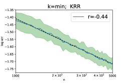
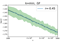
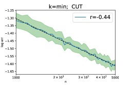
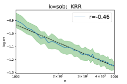
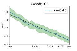
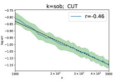
Figure 1: Error decay curves of two kinds of RKHSs and three kinds of spectral algorithms with the best choice of $c$. Both axes are are scaled logarithmically. The curves show the average generalization errors over 50 trials; the regions within one standard deviation are shown in green. The dashed black lines are computed using logarithmic least-squares and the slopes represent the convergence rates $r$. Figures in the first row correspond to the Sobolev RKHS $\mathcal{H}=H^{1}(\mathcal{X})$ and the second correspond to the $\mathcal{H}=\mathcal{H}_{\text{min}}(\mathcal{X})$.

We try different values of $c$, Figure 1 presents the convergence curves under the best choice of $c$. For each setting, it can be concluded that the convergence rates of the $L^{2}$-norm generalization errors of spectral algorithms are indeed approximately equal to $n^{-\frac{s\beta}{s\beta+1}}=n^{-\frac{4}{9}}$, without the boundedness assumption of the true function $f^{*}$. We refer to Appendix C for more details on the experiments.

6 Discussion

In this section, we compare this paper’s convergence rates and minimax optimality with the results in previous literature. Ignoring the log-term and the constants, Theorem 1 gives the upper bound of the convergence rates of spectral algorithms (with high probability)

$$\left\|\hat{f}_{\nu}-f_{\rho}^{*}\right\|_{[\mathcal{H}]^{\gamma}}^{2}\leq\begin{cases}n^{-\frac{(s-\gamma)\beta}{s\beta+1}},\quad&\alpha_{0}-\frac{1}{\beta}<s\leq 2\tau,\\ n^{-\frac{s-\gamma}{\alpha_{0}+\epsilon}},\quad&0<s\leq\alpha_{0}-\frac{1}{\beta},\leavevmode\nobreak\ \leavevmode\nobreak\ \forall\epsilon>0.\end{cases}$$ (19)

This $[\mathcal{H}]^{\gamma}$-norm upper bound depends on $\tau,\beta,s$ and $\alpha_{0}$, among which $\beta,\alpha_{0}$ characterize the information of the RKHS; $s$ characterizes the relative ‘smoothness’ of the true function; and $\tau$ characterizes the spectral algorithm. To our knowledge, this is the most general setting among related literature and will give the most refined analysis. In the well-specified case ($1\leq s\leq 2\tau$ or $f_{\rho}^{*}\in\mathcal{H}$), we recover the well-known minimax optimal rates from a lot of literature (Caponnetto and de Vito, 2007; Caponnetto, 2006; Dicker et al., 2017; Blanchard and Mücke, 2018; Lin et al., 2018; Fischer and Steinwart, 2020, etc.) (for either general spectral algorithms or a specific kind).

The improvement in the misspecified case ($0<s<1$ or $f_{\rho}^{*}\notin\mathcal{H}$) of this paper is partly due to the advantage of considering the embedding index $\alpha_{0}$ of the RKHS. The best upper bound without considering the embedding index is (see, e.g., Dieuleveut and Bach 2016; Lin et al. 2018; Lin and Cevher 2020)

$$\left\|\hat{f}_{\nu}-f_{\rho}^{*}\right\|_{[\mathcal{H}]^{\gamma}}^{2}\leq\begin{cases}n^{-\frac{(s-\gamma)\beta}{s\beta+1}},\quad&1-\frac{1}{\beta}<s\leq 2\tau,\\ n^{-(s-\gamma)},\quad&0<s\leq 1-\frac{1}{\beta}.\end{cases}$$ (20)

This rate coincides with our upper bound (19) if the embedding index $\alpha_{0}=1$. For those RKHSs with $\alpha_{0}<1$, (19) gives refined upper bound for all $0<s\leq 2\tau$. As shown in Section 4, this is the case for many kinds of RKHSs. This is also why we assume $\alpha_{0}\in(0,1)$ throughout our paper.

Compared with the line of work which considers the embedding index (Steinwart and Christmann, 2008; Pillaud-Vivien et al., 2018; Fischer and Steinwart, 2020, etc.), this paper removes the boundedness assumption, i.e., $\|f_{\rho}^{*}\|_{L^{\infty}(\mathcal{X},\mu)}\leq B_{\infty}<\infty$. The upper bound in these works is the same as (19). But due to the boundedness assumption, Fischer and Steinwart (2020) reveals that the minimax lower rate associated to the smaller function space $[\mathcal{H}]^{s}\cap L^{\infty}(\mathcal{X,\mu})$ is larger than

$$n^{-\frac{\max{(s,\alpha)}\beta}{\max{(s,\alpha)}\beta+1}},\quad\forall\alpha>\alpha_{0}.$$

Therefore, they only prove the minimax optimality in the regime

$$\alpha_{0}<s\leq 2\tau.$$

Combining Theorem 1 and Theorem 2, this paper extends the minimax optimality of the spectral algorithms to the regime

$$\alpha_{0}-\frac{1}{\beta}<s\leq 2\tau.$$

This improvement is mainly due to the $L^{q}$-embedding property of the interpolation space $[\mathcal{H}]^{s}$ proved in Theorem 5 and a truncation method in the proof. Note that only the $L^{\infty}$-embedding property has been considered before this paper. This new regime of minimax optimality means a lot. Since we have proved that the embedding index $\alpha_{0}$ equals $\frac{1}{\beta}$ for many kinds of RKHSs, the optimality in the misspecified case is well understood for these RKHSs.

We believe that the new technical tools in this paper can be used for more related topics. For instance, some literature considers the general source condition, i.e.,

$$f_{\rho}^{*}=\phi(L_{k})g_{0},\quad\text{with}\leavevmode\nobreak\ \leavevmode\nobreak\ \|g_{0}\|_{L^{2}}\leq R,$$

where $\phi:\left[0,\kappa^{2}\right]\rightarrow\mathbb{R}^{+}$ is a non-decreasing index function such that $\phi(0)=0$ and $\phi(\kappa^{2})<\infty$ (Bauer et al., 2007; Rastogi and Sampath, 2017; Lin et al., 2018; Talwai and Simchi-Levi, 2022). The source condition in Assumption 3 corresponds to a special choice of $\phi(x)=x^{\frac{s}{2}}$, which is often referred to as the Hölder source condition. Another interesting topic is the distributed version of spectral algorithms (Zhang et al., 2013; Lin et al., 2016; Guo et al., 2017; Mücke and Blanchard, 2018; Lin and Cevher, 2020). It aims to reduce the computation complexity of the original spectral algorithms while maintaining the estimation efficiency. It would be interesting to apply this paper’s tools and try refining the convergence rates or optimality in these scenarios.

In addition, we also notice a line of work which studies the learning curves of kernel ridge regression (Spigler et al., 2020; Bordelon et al., 2020; Cui et al., 2021) and crossovers between different noise magnitudes. At present, their results all rely on a Gaussian design assumption (or some variation), which is a very strong assumption. We believe that studying the misspecified case in our paper is a crucial step to remove the Gaussian design assumption and draw complete conclusions about the learning curves of kernel ridge regression (or further, general spectral algorithms).

The eigenvalue decay rate (also known as the capacity condition or effective dimension condition) and source condition are mentioned in almost all related literature studying the convergence behaviors of kernel methods but are denoted as various kinds of notations. At the end of this section, we list a dictionary of nations in related literature. Recall that in this paper we denote the eigenvalue decay rate as $\beta$ and denote the source condition as $s$. Table 1 summarizes the notations used in some of the references.

$\beta$	$s$	Reference
$1/p$	$\beta$	Steinwart et al. (2009); Fischer and Steinwart (2020); Li et al. (2022)
$1/\gamma$	$2\zeta$	Lin et al. (2018); Lin and Cevher (2020)
$b$	$c$	Caponnetto (2006); Caponnetto and de Vito (2007)
$-$	$2r$	Bauer et al. (2007); Smale and Zhou (2007); Gerfo et al. (2008)
$2\nu$	$\zeta+1$	Dicker et al. (2017)
$b$	$2r+1$	Rastogi and Sampath (2017); Blanchard and Mücke (2018)
$1/b$	$2\beta$	Jun et al. (2019)
$\alpha$	$2r$	Dieuleveut and Bach (2016); Pillaud-Vivien et al. (2018)
		Celisse and Wahl (2020)

Table 1: A dictionary of notations in related literature.

7 Proofs

7.1 $L^{q}-$embedding property of the interpolation space

Before introducing the $L^{q}$-embedding property of the interpolation space $[\mathcal{H}]^{s}$, we first prove the following lemma, which characterizes the real interpolation between two $L^{p}$ spaces with Lorentz space $L^{p,q}(\mathcal{X},\mu)$. We refer to Appendix A for details of real interpolation and Lorentz spaces.

Lemma 4

For $1<p_{1}\neq p_{2}<\infty$, $1\leq q\leq\infty$ and $0<\theta<1$, we have

$$\left(L^{p_{1}}(\mathcal{X},\mu),L^{p_{2}}(\mathcal{X},\mu)\right)_{\theta,q}=L^{p_{\theta},q}(\mathcal{X},\mu),\quad\frac{1}{p_{\theta}}=\frac{1-\theta}{p_{1}}+\frac{\theta}{p_{2}},$$

where $L^{p_{\theta},q}(\mathcal{X},\mu)$ is the Lorentz space.

Proof  Denote $L^{p}(\mathcal{X},\mu),L^{p,q}(\mathcal{X},\mu)$ as $L^{p},L^{p,q}$ for brevity. Using Lemma 29, we know that $L^{p_{i}}\cong L^{p_{i},p_{i}}=\left(L^{1},L^{\infty}\right)_{\frac{1}{p_{i}^{\prime}},p_{i}}$, where $\frac{1}{p_{i}^{\prime}}+\frac{1}{p_{i}}=1,i=1,2.$ Since $1<p_{i}<\infty,i=1,2$, Lemma 24 implies that

$$\left(L^{1},L^{\infty}\right)_{\frac{1}{p_{1}^{\prime}},1} \subset L^{p_{1}}\subset\left(L^{1},L^{\infty}\right)_{\frac{1}{p_{1}^{\prime}},\infty};$$

$$\left(L^{1},L^{\infty}\right)_{\frac{1}{p_{2}^{\prime}},1} \subset L^{p_{2}}\subset\left(L^{1},L^{\infty}\right)_{\frac{1}{p_{2}^{\prime}},\infty}.$$

Using the Reiteration theorem (Theorem 26), we have

$$\left(L^{p_{1}},L^{p_{2}}\right)_{\theta,q}=\left(L^{1},L^{\infty}\right)_{\eta,q},$$ (21)

where $\eta=\frac{1-\theta}{p_{1}^{\prime}}+\frac{\theta}{p_{2}^{\prime}}$. Simple calculations show that

$$1-\eta=\frac{1-\theta}{p_{1}}+\frac{\theta}{p_{2}}:=\frac{1}{p_{\theta}}.$$

So by the definition of Lorentz space, we have

$$\left(L^{1},L^{\infty}\right)_{\eta,q}=L^{\frac{1}{1-\eta},q}=L^{p_{\theta},q}.$$

Together with (21), we finish the proof.  

Based on Lemma 4, the following theorem gives the $L^{q}$-embedding property of the interpolation space of an RKHS $\mathcal{H}$, which is crucial for proving the upper bound.

Theorem 5 ($L^{q}$-embedding property)

Suppose that the RKHS $\mathcal{H}$ has embedding index $\alpha_{0}$, then for any $0<s\leq\alpha_{0}$, we have

$$[\mathcal{H}]^{s}\hookrightarrow L^{q_{s}}(\mathcal{X},\mu),\quad q_{s}=\frac{2\alpha}{\alpha-s},\quad\forall\alpha>\alpha_{0}.$$

where $\hookrightarrow$ denotes the continuous embedding.

Proof 

Since the embedding index is $\alpha_{0}$, we know that $[\mathcal{H}]^{\alpha^{\prime}}\hookrightarrow L^{\infty}(\mathcal{X},\mu),\forall\alpha^{\prime}>\alpha_{0}$. In addition, (7) shows that

$$[\mathcal{H}]^{s}=\big{[}\left[\mathcal{H}\right]^{\alpha^{\prime}}\big{]}^{\frac{s}{\alpha^{\prime}}}\cong\left(L^{2}(\mathcal{X},\mu),\left[\mathcal{H}\right]^{\alpha^{\prime}}\right)_{\frac{s}{\alpha^{\prime}},2}.$$

So using Lemma 4, for any $0<M<\infty$, we have

$$[\mathcal{H}]^{s}\hookrightarrow\left(L^{2}(\mathcal{X},\mu),L^{M}(\mathcal{X},\mu)\right)_{\frac{s}{\alpha^{\prime}},2}\cong L^{q_{s}^{\prime},2}(\mathcal{X},\mu),$$

where $\frac{1}{q_{s}^{\prime}}=\frac{1-\frac{s}{\alpha^{\prime}}}{2}+\frac{\frac{s}{\alpha^{\prime}}}{M}=\frac{\alpha^{\prime}-s}{2\alpha^{\prime}}+\frac{s}{\alpha^{\prime}M}$.

For any $\alpha>\alpha_{0}$, we can choose the above $\alpha^{\prime}\in\left(\alpha_{0},\alpha\right)$ and $M$ large enough such that $\frac{\alpha^{\prime}-s}{2\alpha^{\prime}}+\frac{s}{\alpha^{\prime}M}<\frac{\alpha-s}{2\alpha}$. Letting $q_{s}=\frac{2\alpha}{\alpha-s}$, we have $q_{s}^{\prime}>q_{s}$. Further, since $0<s\leq\alpha_{0}<\alpha$ thus $q_{s}^{\prime}>q_{s}>2$, using Lemma 24 and Lemma 29, we have

$$L^{q_{s}^{\prime},2}(\mathcal{X},\mu)\hookrightarrow L^{q_{s}^{\prime},q_{s}^{\prime}}(\mathcal{X},\mu)\cong L^{q_{s}^{\prime}}(\mathcal{X},\mu)\hookrightarrow L^{q_{s}}(\mathcal{X},\mu).$$

We finish the proof.

 

7.2 Some bounds

Throughout the proof, we denote

$$T_{\nu}=T+\nu^{-1};\leavevmode\nobreak\ \leavevmode\nobreak\ T_{X\nu}=T_{X}+\nu^{-1},$$

where $\nu$ is the regularization parameter. We use $\|\cdot\|_{\mathscr{B}(B_{1},B_{2})}$ to denote the operator norm of a bounded linear operator from a Banach space $B_{1}$ to $B_{2}$, i.e., $\|A\|_{\mathscr{B}(B_{1},B_{2})}=\sup\limits_{\|f\|_{B_{1}}=1}\|Af\|_{B_{2}}$. Without bringing ambiguity, we will briefly denote the operator norm as $\|\cdot\|$. In addition, we use $\text{tr}A$ and $\|A\|_{1}$ to denote the trace and the trace norm of an operator. We use $\|A\|_{2}$ to denote the Hilbert-Schmidt norm. In addition, we denote $L^{2}(\mathcal{X},\mu)$ as $L^{2}$, $L^{\infty}(\mathcal{X},\mu)$ as $L^{\infty}$ for brevity throughout the proof. We use $a_{n}\asymp b_{n}$ to denote that there exist constants $c$ and $C$ such that $ca_{n}\leq b_{n}\leq Ca_{n},\forall n=1,2,\cdots$; use $a_{n}\lesssim b_{n}$ to denote that there exists an constant $C$ such that $a_{n}\leq Cb_{n},\forall n=1,2,\cdots$

In addition, denote the effective dimension as

$$\mathcal{N}(\nu)=\text{tr}\big{(}T(T+\nu^{-1})^{-1}\big{)}=\sum\limits_{i\in N}\frac{\lambda_{i}}{\lambda_{i}+\nu^{-1}}.$$

Since the EDR of $\mathcal{H}$ is $\beta$, Lemma 31 shows that $\mathcal{N}(\nu)\asymp\nu^{\frac{1}{\beta}}$.

Recall that we have define the sample basis function $g_{Z}$ and the spectral algorithm $\hat{f}_{\nu}$ in Section 2.2. We also need the following notations: define the expectation of $g_{Z}$ as

$$g=\mathbb{E}g_{Z}=\int_{\mathcal{X}}k(x,\cdot)f_{\rho}^{*}(x)d\mu(x)=S_{k}^{*}f_{\rho}^{*}\in\mathcal{H},$$

and

$$f_{\nu}=\varphi_{\nu}(T)g=\varphi_{\nu}(T)S_{k}^{*}f_{\rho}^{*}.$$

The following theorem bounds the $[\mathcal{H}]^{\gamma}$-norm of $f_{\nu}-f_{\rho}^{*}$ when $0\leq\gamma\leq s$.

Theorem 6

Suppose that Assumption 3 holds for $0<s\leq 2\tau$. Then for any $\nu>0$ and $0\leq\gamma\leq s$, we have

$$\left\|f_{\nu}-f_{\rho}^{*}\right\|_{[\mathcal{H}]^{\gamma}}\leq F_{\tau}R\nu^{-\frac{s-\gamma}{2}}.$$ (22)

Proof  Suppose that $f_{\rho}^{*}=L_{k}^{\frac{s}{2}}g_{0}$ for some $g_{0}\in L^{2}$. Note that

$$\left\|f_{\nu}-f_{\rho}^{*}\right\|_{[\mathcal{H}]^{\gamma}} =\left\|L_{k}^{-\frac{\gamma}{2}}\left(S_{k}\varphi_{\nu}(T)S_{k}^{*}f_{\rho}^{*}-f_{\rho}^{*}\right)\right\|_{L^{2}}$$

$$=\left\|L_{k}^{-\frac{\gamma}{2}}\left(\varphi_{\nu}(L_{k})L_{k}-I\right)L_{k}^{\frac{s}{2}}g_{0}\right\|_{L^{2}}$$

$$\leq\left\|L_{k}^{\frac{s-\gamma}{2}}\psi_{\nu}(L_{k})\right\|R$$

$$\leq F_{\tau}R\nu^{-\frac{s-\gamma}{2}},$$

where we use the property of the filter function (10) and $\left\|g_{0}\right\|_{L^{2}}=\|f_{\rho}^{*}\|_{[\mathcal{H}]^{s}}\leq R$ for the last inequality.  

The following lemma bounds the $L^{\infty}$-norm of $f_{\nu}$ when $s\leq\alpha_{0}$.

Lemma 7

Suppose that Assumption 1, 2 and 3 hold for $0<s\leq\alpha_{0}$ and $\frac{1}{\beta}\leq\alpha_{0}<1$. Then for any $\nu>0$ and any $\alpha_{0}<\alpha\leq 1$, we have

$$\|f_{\nu}\|_{L^{\infty}}\leq M_{\alpha}ER\nu^{\frac{\alpha-s}{2}}.$$ (23)

Proof  Since $s\leq\alpha_{0}$ and $\alpha>\alpha_{0}$, we have

$$\left\|f_{\nu}\right\|_{[\mathcal{H}]^{\alpha}} =\left\|L_{k}^{-\frac{\alpha}{2}}S_{k}\varphi_{\nu}(T)S_{k}^{*}f_{\rho}^{*}\right\|_{[\mathcal{H}]^{\alpha}}$$

$$=\left\|L_{k}^{-\frac{\alpha}{2}}\varphi_{\nu}(L_{k})L_{k}L_{k}^{\frac{s}{2}}g_{0}\right\|_{L^{2}}$$

$$=\left\|L_{k}^{1-\frac{\alpha-s}{2}}\varphi_{\nu}(L_{k})g_{0}\right\|_{L^{2}}$$

$$=\left\|L_{k}^{1-\frac{\alpha-s}{2}}\varphi_{\nu}(L_{k})\right\|\left\|g_{0}\right\|_{L^{2}}$$

$$\leq ER\nu^{\frac{\alpha-s}{2}},$$

where we use the property of the filter function (9) for the last inequality. Further, using $\|[\mathcal{H}]^{\alpha}\hookrightarrow L^{\infty}(\mathcal{X},\mu)\|=M_{\alpha}$ by Assumption 2, we have $\|f_{\nu}\|_{L^{\infty}}\leq M_{\alpha}\|f_{\nu}\|_{[\mathcal{H}]^{\alpha}}\leq M_{\alpha}ER\nu^{\frac{\alpha-s}{2}}$.  

The following lemma will be frequently used in our proof.

Lemma 8

Suppose that the RKHS $\mathcal{H}$ has embedding index $\alpha_{0}$. For any $\alpha_{0}<\alpha\leq 1$, we have

$$\|T_{\nu}^{-\frac{1}{2}}k(x,\cdot)\|_{\mathcal{H}}^{2}\leq M_{\alpha}^{2}\nu^{\alpha},\quad\mu\text{-a.e. }x\in\mathcal{X}.$$ (24)

Proof  Recalling the definition of the embedding index, for any $\alpha_{0}<\alpha\leq 1$,

$$\sum_{i\in N}\lambda_{i}^{\alpha}e_{i}^{2}(x)\leq M_{\alpha},\quad\mu\text{-a.e. }x\in\mathcal{X}.$$

So, we have

$$\|T_{\nu}^{-\frac{1}{2}}k(x,\cdot)\|_{\mathcal{H}}^{2} =\Big{\|}\sum\limits_{i\in N}(\frac{1}{\lambda_{i}+\nu^{-1}})^{\frac{1}{2}}\lambda_{i}e_{i}(x)e_{i}(\cdot)\Big{\|}_{\mathcal{H}}^{2}$$

$$=\sum\limits_{i\in N}\frac{\lambda_{i}}{\lambda_{i}+\nu^{-1}}e_{i}^{2}(x)$$

$$=\big{[}\sum\limits_{i\in N}\lambda_{i}^{\alpha}e_{i}^{2}(x)\big{]}\sup\limits_{i\in N}\frac{\lambda_{i}^{1-\alpha}}{\lambda_{i}+\nu^{-1}}$$

$$\leq M_{\alpha}^{2}\nu^{\alpha},\quad\mu\text{-a.e. }x\in\mathcal{X}.$$

where we use Lemma 30 for the last inequality and we finish the proof.  

Lemma 8 has a direct corollary.

Lemma 9

Suppose that the RKHS $\mathcal{H}$ has embedding index $\alpha_{0}$. For any $\alpha_{0}<\alpha\leq 1$, we have

$$\|T_{\nu}^{-\frac{1}{2}}T_{x}T_{\nu}^{-\frac{1}{2}}\|\leq M_{\alpha}^{2}\nu^{\alpha},\quad\mu\text{-a.e. }x\in\mathcal{X}.$$

Proof  Note that for any $f\in\mathcal{H}$,

$$T_{\nu}^{-\frac{1}{2}}T_{x}T_{\nu}^{-\frac{1}{2}}f =T_{\nu}^{-\frac{1}{2}}K_{x}K_{x}^{*}T_{\nu}^{-\frac{1}{2}}f$$

$$=T_{\nu}^{-\frac{1}{2}}K_{x}\langle k(x,\cdot),T_{\nu}^{-\frac{1}{2}}f\rangle_{\mathcal{H}}$$

$$=T_{\nu}^{-\frac{1}{2}}K_{x}\langle T_{\nu}^{-\frac{1}{2}}k(x,\cdot),f\rangle_{\mathcal{H}}$$

$$=\langle T_{\nu}^{-\frac{1}{2}}k(x,\cdot),f\rangle_{\mathcal{H}}\cdot T_{\nu}^{-\frac{1}{2}}k(x,\cdot).$$

So $\|T_{\nu}^{-\frac{1}{2}}T_{x}T_{\nu}^{-\frac{1}{2}}\|=\sup\limits_{\|f\|_{\mathcal{H}}=1}\|T_{\nu}^{-\frac{1}{2}}T_{x}T_{\nu}^{-\frac{1}{2}}f\|_{\mathcal{H}}=\sup\limits_{\|f\|_{\mathcal{H}}=1}\langle T_{\nu}^{-\frac{1}{2}}k(x,\cdot),f\rangle_{\mathcal{H}}\cdot\|T_{\nu}^{-\frac{1}{2}}k(x,\cdot)\|_{\mathcal{H}}=\|T_{\nu}^{-\frac{1}{2}}k(x,\cdot)\|_{\mathcal{H}}^{2}$. Using Lemma 8, we finish the proof.  

The following lemma is a corollary of Lemma 33, which is also used in Lin et al. (2018, Lemma 5.5) and Smale and Zhou (2007).

Lemma 10

Let $0<\delta<\frac{1}{2}$, it holds with probability at least $1-\delta$

$$\left\|T_{X}-T\right\|\leq\left\|T_{X}-T\right\|_{2}\leq\frac{8\sqrt{2}\kappa^{2}}{\sqrt{n}}\ln\frac{2}{\delta},$$

where $\|\cdot\|$ denotes the operator norm and $\|\cdot\|_{2}$ denotes the Hilbert-Schmidt norm.

Proof  Define $\xi(x)=T_{x}$, then we have

$$T_{X}-T=\frac{1}{n}\sum\limits_{i=1}^{n}\xi(x_{i})-\mathbb{E}\xi(x).$$

Since $\sup\limits_{x\in\mathcal{X}}k(x,x)\leq\kappa^{2}$, the Hilbert-Schmidt norm of $\xi(x)$ satisfies that

$$\left\|\xi(x)\right\|_{2}\leq\kappa^{2},\quad\forall x\in\mathcal{X}.$$

Applying Lemma 33 with $L=\sigma=\kappa^{2}$, with probability at least $1-\delta$, we have

$$\left\|T_{X}-T\right\|_{2}\leq 4\sqrt{2}\ln{\frac{2}{\delta}}\left(\frac{\kappa^{2}}{n}+\frac{\kappa^{2}}{\sqrt{n}}\right)\leq\frac{8\sqrt{2}\kappa^{2}}{\sqrt{n}}\ln\frac{2}{\delta}.$$

The first inequality follows from the fact that $\left\|T_{X}-T\right\|\leq\left\|T_{X}-T\right\|_{2}$.  

7.3 Upper bound

Lemma 11

Suppose that the RKHS $\mathcal{H}$ has embedding index $\alpha_{0}$. Then for any $\alpha_{0}<\alpha\leq 1$ and all $\delta\in(0,1)$, with probability at least $1-\delta$, we have

$$\|T_{\nu}^{-\frac{1}{2}}(T-T_{X})T_{\nu}^{-\frac{1}{2}}\|\leq\frac{4M_{\alpha}^{2}\nu^{\alpha}}{3n}B+\sqrt{\frac{2M_{\alpha}^{2}\nu^{\alpha}}{n}B},$$

where

$$B=\ln{\frac{4\mathcal{N}(\nu)(\|T\|+\nu^{-1})}{\delta\|T\|}}.$$

Proof  Denote $A_{i}=T_{\nu}^{-\frac{1}{2}}(T-T_{x_{i}})T_{\nu}^{-\frac{1}{2}}$, using Lemma 9, we have

$$\|A_{i}\|=\|T_{\nu}^{-\frac{1}{2}}TT_{\nu}^{-\frac{1}{2}}\|+\|T_{\nu}^{-\frac{1}{2}}T_{x_{i}}T_{\nu}^{-\frac{1}{2}}\|\leq 2M_{\alpha}^{2}\nu^{\alpha},\quad\mu\text{-a.e. }x\in\mathcal{X}.$$

We use $A\preceq B$ to denote that $A-B$ is a positive semi-definite operator. Using the fact that $\mathbb{E}(B-\mathbb{E}B)^{2}\preceq\mathbb{E}B^{2}$ for a self-adjoint operator $B$, we have

$$\mathbb{E}A_{i}^{2}\preceq\mathbb{E}\left[T_{\nu}^{-\frac{1}{2}}T_{x_{i}}T_{\nu}^{-\frac{1}{2}}\right]^{2}.$$

In addition, Lemma 9 shows that $0\preceq T_{\nu}^{-\frac{1}{2}}T_{x_{i}}T_{\nu}^{-\frac{1}{2}}\preceq M_{\alpha}^{2}\nu^{\alpha},\mu\text{-a.e. }x\in\mathcal{X}$. So we have

$$\mathbb{E}A_{i}^{2}\preceq\mathbb{E}\left[T_{\nu}^{-\frac{1}{2}}T_{x_{i}}T_{\nu}^{-\frac{1}{2}}\right]^{2}\preceq\mathbb{E}\left[M_{\alpha}^{2}\nu^{\alpha}\cdot T_{\nu}^{-\frac{1}{2}}T_{x_{i}}T_{\nu}^{-\frac{1}{2}}\right]=M_{\alpha}^{2}\nu^{\alpha}T_{\nu}^{-1}T,$$

Define an operator $V:=M_{\alpha}^{2}\nu^{\alpha}T_{\nu}^{-1}T$, we have

$$\|V\| =M_{\alpha}^{2}\nu^{\alpha}\frac{\lambda_{1}}{\lambda_{1}+\nu^{-1}}=M_{\alpha}^{2}\nu^{\alpha}\frac{\|T\|}{\|T\|+\nu^{-1}}\leq M_{\alpha}^{2}\nu^{\alpha};$$

$$\text{tr}V =M_{\alpha}^{2}\nu^{\alpha}\mathcal{N}(\nu);$$

$$\frac{\text{tr}V}{\|V\|} =\frac{\mathcal{N}(\nu)(\|T\|+\nu^{-1})}{\|T\|}.$$

Use Lemma 32 to $A_{i}$, $V$ and we finish the proof.  

Lemma 12

Suppose that the RKHS $\mathcal{H}$ has embedding index $\alpha_{0}$. For any $\alpha_{0}<\alpha\leq 1$, if $\nu$ and $n$ satisfy that

$$\frac{M_{\alpha}^{2}\nu^{\alpha}}{n}\ln\frac{4\kappa^{2}\mathcal{N}(\nu)\left(\|T\|+\nu^{-1}\right)}{\delta\|T\|}\leq\frac{1}{8},$$ (25)

then for all $\delta\in(0,1)$, with probability at least $1-\delta$, we have

$$\left\|T_{\nu}^{-\frac{1}{2}}T_{X\nu}^{\frac{1}{2}}\right\|^{2}\leq 2,\quad\left\|T_{\nu}^{\frac{1}{2}}T_{X\nu}^{-\frac{1}{2}}\right\|^{2}\leq 3.$$

Proof  Define

$$u=\frac{M_{\alpha}^{2}\nu^{\alpha}}{n}\ln\frac{4\kappa^{2}\mathcal{N}(\nu)\left(\|T\|+\nu^{-1}\right)}{\delta\|T\|}\leq\frac{1}{8}.$$

Using Lemma 11, with probability at least $1-\delta$, we have

$$a:=\|T_{\nu}^{-\frac{1}{2}}(T-T_{X})T_{\nu}^{-\frac{1}{2}}\|\leq\frac{4}{3}u+\sqrt{2u}\leq\frac{2}{3}.$$

So we have

$$\left\|T_{\nu}^{-\frac{1}{2}}T_{X\nu}^{\frac{1}{2}}\right\|^{2} =\left\|T_{\nu}^{-\frac{1}{2}}T_{X\nu}T_{\nu}^{-\frac{1}{2}}\right\|=\left\|T_{\nu}^{-\frac{1}{2}}\left(T_{X}+\nu^{-1}\right)T_{\nu}^{-\frac{1}{2}}\right\|$$

$$=\left\|T_{\nu}^{-\frac{1}{2}}\left(T_{X}-T+T+\nu^{-1}\right)T_{\nu}^{-\frac{1}{2}}\right\|$$

$$=\left\|T_{\nu}^{-\frac{1}{2}}\left(T_{X}-T\right)T_{\nu}^{-\frac{1}{2}}+I\right\|$$

$$\leq a+1\leq 2;$$

and

$$\left\|T_{\nu}^{\frac{1}{2}}T_{X\nu}^{-\frac{1}{2}}\right\|^{2} =\left\|T_{\nu}^{\frac{1}{2}}T_{X\nu}^{-1}T_{\nu}^{\frac{1}{2}}\right\|=\left\|\left(T_{\nu}^{-\frac{1}{2}}T_{X\nu}T_{\nu}^{-\frac{1}{2}}\right)^{-1}\right\|$$

$$=\left\|\left(I-T_{\nu}^{-\frac{1}{2}}(T_{X}-T)T_{\nu}^{-\frac{1}{2}}\right)^{-1}\right\|$$

$$\leq\sum\limits_{k=0}^{\infty}\left\|T_{\nu}^{-\frac{1}{2}}(T_{X}-T)T_{\nu}^{-\frac{1}{2}}\right\|^{k}$$

$$\leq\sum\limits_{k=0}^{\infty}\left(\frac{2}{3}\right)^{k}\leq 3.$$

 

The following theorem is an application of the classical Bernstein inequality but considering a truncation version of $f_{\rho}^{*}$, which will bring refined analysis when handling those $f_{\rho}^{*}\notin L^{\infty}$.

Theorem 13

Suppose that Assumption 1, 2, 3 and 4 hold for $0<s\leq 2\tau$ and $\frac{1}{\beta}\leq\alpha_{0}<1$. Denote $\xi_{i}=\xi(x_{i},y_{i})=T_{\nu}^{-\frac{1}{2}}(K_{x_{i}}y_{i}-T_{x_{i}}f_{\nu})$ and $\Omega_{0}=\{x\in\mathcal{X}:|f_{\rho}^{*}(x)|\leq t\}$. Then for any $\alpha_{0}<\alpha\leq 1$ and all $\delta\in(0,1)$, with probability at least $1-\delta$, we have

$$\left\|\frac{1}{n}\sum\limits_{i=1}^{n}\xi_{i}I_{x_{i}\in\Omega_{0}}-\mathbb{E}\xi_{x}I_{x\in\Omega_{0}}\right\|_{\mathcal{H}}\leq\ln\frac{2}{\delta}\left(\frac{C_{1}\nu^{\frac{\alpha}{2}}}{n}\cdot\tilde{M}+\frac{C_{2}\mathcal{N}^{\frac{1}{2}}(\nu)}{\sqrt{n}}+\frac{C_{3}\nu^{\frac{\alpha-s}{2}}}{\sqrt{n}}\right),$$

where $\tilde{M}=M_{\alpha}(E+F_{\tau})R\nu^{\frac{\alpha-s}{2}}+t+L$ and $L$ is the constant in (4). $C_{1}=8\sqrt{2}M_{\alpha},C_{2}=8\sigma,C_{3}=8\sqrt{2}M_{\alpha}F_{\tau}R$.

Proof  Note that $f_{\rho}^{*}$ can represent a $\mu$-equivalence class in $L^{2}(\mathcal{X},\mu)$. When defining the set $\Omega_{0}$, we actually denote $f_{\rho}^{*}$ as the representative $f_{\rho}^{*}(x)=\int_{\mathcal{Y}}y\mathrm{d}\rho(y|x).$

To use Lemma 33, we need to bound the m-th moment of $\xi(x,y)I_{x\in\Omega_{0}}$.

$$\mathbb{E}\left\|\xi(x,y)I_{x\in\Omega_{0}}\right\|_{\mathcal{H}}^{m} =\mathbb{E}\left\|T_{\nu}^{-\frac{1}{2}}K_{x}(y-f_{\nu}(x))I_{x\in\Omega_{0}}\right\|_{\mathcal{H}}^{m}$$

$$\leq\mathbb{E}\Big{(}\left\|T_{\nu}^{-\frac{1}{2}}k(x,\cdot)\right\|_{\mathcal{H}}^{m}\mathbb{E}\big{(}\left|(y-f_{\nu}(x))I_{x\in\Omega_{0}}\right|^{m}\leavevmode\nobreak\ \big{|}\leavevmode\nobreak\ x\big{)}\Big{)}.$$ (26)

Using the inequality $(a+b)^{m}\leq 2^{m-1}\left(a^{m}+b^{m}\right)$, we have

$$\left|y-f_{\nu}(x)\right|^{m} \leq 2^{m-1}\left(\left|f_{\nu}(x)-f_{\rho}^{*}(x)\right|^{m}+\left|f_{\rho}^{*}(x)-y\right|^{m}\right)$$

$$=2^{m-1}\left(\left|f_{\nu}(x)-f_{\rho}^{*}(x)\right|^{m}+|\epsilon|^{m}\right).$$ (27)

Plugging (7.3) into (7.3), we have

$$\mathbb{E}\left\|\xi(x,y)I_{x\in\Omega_{0}}\right\|_{\mathcal{H}}^{m}\leavevmode\nobreak\ \leq\leavevmode\nobreak\ 2^{m-1}\mathbb{E}\Big{(}\left\|T_{\nu}^{-\frac{1}{2}}k(x,\cdot)\right\|_{\mathcal{H}}^{m}\left|(f_{\nu}(x)-f_{\rho}^{*}(x))I_{x\in\Omega_{0}}\right|^{m}\Big{)}$$ (28)

$$+2^{m-1}\mathbb{E}\Big{(}\left\|T_{\nu}^{-\frac{1}{2}}k(x,\cdot)\right\|_{\mathcal{H}}^{m}\mathbb{E}\big{(}\left|\epsilon\leavevmode\nobreak\ I_{x\in\Omega_{0}}\right|^{m}\leavevmode\nobreak\ \big{|}\leavevmode\nobreak\ x\big{)}\Big{)}$$ (29)

Now we begin to bound (29). Note that we have proved in Lemma 8 that for $\mu$-almost $x\in\mathcal{X}$,

$$\left\|T_{\nu}^{-\frac{1}{2}}k(x,\cdot)\right\|_{\mathcal{H}}\leq M_{\alpha}\nu^{\frac{\alpha}{2}};$$

In addition, we also have

$$\mathbb{E}\left\|T_{\nu}^{-\frac{1}{2}}k(x,\cdot)\right\|_{\mathcal{H}}^{2} =\mathbb{E}\Big{\|}\sum\limits_{i\in N}(\frac{1}{\lambda_{i}+\nu^{-1}})^{\frac{1}{2}}\lambda_{i}e_{i}(x)e_{i}(\cdot)\Big{\|}_{\mathcal{H}}^{2}$$

$$=\mathbb{E}\Big{(}\sum\limits_{i\in N}\frac{\lambda_{i}}{\lambda_{i}+\nu^{-1}}e_{i}^{2}(x)\Big{)}$$

$$=\sum\limits_{i\in N}\frac{\lambda_{i}}{\lambda_{i}+\nu^{-1}}$$

$$=\mathcal{N}(\nu).$$

So we have

$$\mathbb{E}\left\|T_{\nu}^{-\frac{1}{2}}k(x,\cdot)\right\|_{\mathcal{H}}^{m}\leq\left(M_{\alpha}\nu^{\frac{\alpha}{2}}\right)^{m-2}\cdot\mathbb{E}\left\|T_{\nu}^{-\frac{1}{2}}k(x,\cdot)\right\|_{\mathcal{H}}^{2}=\big{(}M_{\alpha}\nu^{\frac{\alpha}{2}}\big{)}^{m-2}\mathcal{N}(\nu).$$

Using Assumption 4, we have

$$\mathbb{E}\left(|\epsilon I_{x\in\Omega_{0}}|^{m}\mid x\right)\leq\mathbb{E}\left(|\epsilon|^{m}\mid x\right)\leq\frac{1}{2}m!\sigma^{2}L^{m-2},\quad\mu\text{-a.e. }x\in\mathcal{X},$$

so we get the upper bound of (29), i.e.,

$$(\ref{proof of 4.9-3})\leq\frac{1}{2}m!\left(\sqrt{2}\sigma\mathcal{N}^{\frac{1}{2}}(\nu)\right)^{2}(2M_{\alpha}\nu^{\frac{\alpha}{2}}L)^{m-2}.$$

Now we begin to bound (28).

• When $s\leq\alpha_{0}$, using the definition of $\Omega_{0}$ and Lemma 7, we have

  $$\|(f_{\nu}-f_{\rho}^{*})I_{x\in\Omega_{0}}\|_{L^{\infty}}\leq\|f_{\nu}\|_{L^{\infty}}+\|f_{\rho}^{*}I_{x\in\Omega_{0}}\|_{L^{\infty}}\leq M_{\alpha}ER\nu^{\frac{\alpha-s}{2}}+t.$$ (30)

• When $s>\alpha_{0}$, without loss of generality, we assume $\alpha_{0}<\alpha\leq s$. using Theorem 6 for $\gamma=\alpha$, we have

  $$\|(f_{\nu}-f_{\rho}^{*})I_{x\in\Omega_{0}}\|_{L^{\infty}}\leq M_{\alpha}\|f_{\nu}-f_{\rho}^{*}\|_{[\mathcal{H}]^{\alpha}}\leq M_{\alpha}F_{\tau}R\nu^{\frac{\alpha-s}{2}}.$$ (31)

Therefore, (30) and (31) imply that for all $0<s\leq 2$ we have

$$\|(f_{\nu}-f_{\rho}^{*})I_{x\in\Omega_{0}}\|_{L^{\infty}}\leq M_{\alpha}(E+F_{\tau})R\nu^{\frac{\alpha-s}{2}}+t:=M.$$ (32)

In addition, using Theorem 6 for $\gamma=0$, we also have

$$\mathbb{E}|(f_{\nu}(x)-f_{\rho}^{*}(x))I_{x\in\Omega_{0}}|^{2}\leq\mathbb{E}|f_{\nu}(x)-f_{\rho}^{*}(x)|^{2}\leq(F_{\tau}R\nu^{-\frac{s}{2}})^{2}.$$

So we get the upper bound of (28), i.e.,

$$(\ref{proof of 4.9-2}) \leq 2^{m-1}(M_{\alpha}\nu^{\frac{\alpha}{2}})^{m}\cdot\|(f_{\nu}-f_{\rho}^{*})I_{x\in\Omega_{0}}\|_{L^{\infty}}^{m-2}\cdot\mathbb{E}|(f_{\nu}(x)-f_{\rho}^{*}(x))I_{x\in\Omega_{0}}|^{2}$$

$$\leq 2^{m-1}(M_{\alpha}\nu^{\frac{\alpha}{2}})^{m}\cdot M^{m-2}\cdot(F_{\tau}R\nu^{-\frac{s}{2}})^{2}$$

$$\leq\frac{1}{2}m!\big{(}2M_{\alpha}\nu^{\frac{\alpha}{2}}M\big{)}^{m-2}\big{(}2M_{\alpha}F_{\tau}R\nu^{\frac{\alpha-s}{2}}\big{)}^{2}.$$

Denote

$$\tilde{L} =2M_{\alpha}(M+L)\nu^{\frac{\alpha}{2}}$$

$$\tilde{\sigma} =2M_{\alpha}F_{\tau}R\nu^{\frac{\alpha-s}{2}}+\sqrt{2}\sigma\mathcal{N}^{\frac{1}{2}}(\nu),$$

then the bounds of (28) and (29) show that $\mathbb{E}\left\|\xi(x,y)I_{x\in\Omega_{0}}\right\|_{\mathcal{H}}^{m}\leq\frac{1}{2}m!\tilde{\sigma}^{2}\tilde{L}^{m-2}$. Using Lemma 33, we finish the proof.  

Remark 14

In fact, when we later applying Theorem 13 in the proof of Theorem 15, the truncation in this theorem is necessary only in the $s\leq\alpha_{0}$ case. But for the completeness and consistency of our proof, we also include $s>\alpha_{0}$ in this theorem.

Based on Theorem 13, the following theorem will give an upper bound of

$$\left\|T_{\nu}^{-\frac{1}{2}}\left[\left(g_{Z}-T_{X}f_{\nu}\right)-\left(g-Tf_{\nu}\right)\right]\right\|_{\mathcal{H}}.$$

Theorem 15

Suppose that Assumption 1, 2, 3 and 4 hold for $0<s\leq 2\tau$ and $\frac{1}{\beta}\leq\alpha_{0}<1$.

• In the case of $s+\frac{1}{\beta}>\alpha_{0}$, by choosing $\nu\asymp n^{\frac{\beta}{s\beta+1}}$, for any fixed $\delta\in(0,1)$, when $n$ is sufficiently large, with probability at least $1-\delta$ , we have

  $$\left\|T_{\nu}^{-\frac{1}{2}}\left[\left(g_{Z}-T_{X}f_{\nu}\right)-\left(g-Tf_{\nu}\right)\right]\right\|_{\mathcal{H}}\leq\ln{\frac{2}{\delta}}C\frac{\nu^{\frac{1}{2\beta}}}{\sqrt{n}}=\ln{\frac{2}{\delta}}Cn^{-\frac{1}{2}\frac{s\beta}{s\beta+1}},$$ (33)

  where $C$ is a constant independent of $n$ and $\delta$.

• In the case of $s+\frac{1}{\beta}\leq\alpha_{0}$, for any $\alpha_{0}<\alpha\leq 1$, by choosing $\nu\asymp(\frac{n}{\ln^{r}(n)})^{\frac{1}{\alpha}}$, for some $r>1$, for any fixed $\delta\in(0,1)$, when $n$ is sufficiently large, with probability at least $1-\delta$, we have

  $$\left\|T_{\nu}^{-\frac{1}{2}}\left[\left(g_{Z}-T_{X}f_{\nu}\right)-\left(g-Tf_{\nu}\right)\right]\right\|_{\mathcal{H}}\leq\ln{\frac{2}{\delta}}C\frac{\nu^{\frac{\alpha-s}{2}}}{\sqrt{n}}\leq\ln{\frac{2}{\delta}}C\left(\frac{n}{\ln^{r}(n)}\right)^{-\frac{1}{2}\frac{s}{\alpha}},$$ (34)

  where $C$ is a constant independent of $n$ and $\delta$.

Proof 

The $\bm{s+\frac{1}{\beta}>\alpha_{0}}$ case:

Denote $\xi_{i}=\xi(x_{i},y_{i})=T_{\nu}^{-\frac{1}{2}}(K_{x_{i}}y_{i}-T_{x_{i}}f_{\nu})$, (33) is equivalent to

$$\left\|\frac{1}{n}\sum\limits_{i=1}^{n}\xi_{i}-\mathbb{E}\xi_{x}\right\|_{\mathcal{H}}\leq\ln{\frac{2}{\delta}}C\frac{\nu^{\frac{1}{2\beta}}}{\sqrt{n}}=\ln{\frac{2}{\delta}}Cn^{-\frac{1}{2}\frac{s\beta}{s\beta+1}}.$$ (35)

Consider the subset $\Omega_{1}=\{x\in\mathcal{X}:|f_{\rho}^{*}(x)|\leq t\}$ and $\Omega_{2}=\mathcal{X}\backslash\Omega_{1}$, where $t$ will be chosen appropriately later. Assume that for some $q\geq 2$,

$$[\mathcal{H}]^{s}\hookrightarrow L^{q}(\mathcal{X},\mu).$$

Then Assumption 3 shows that there exists $0<C_{q}<\infty$ such that $\|f_{\rho}^{*}\|_{L^{q}(\mathcal{X},\mu)}\leq C_{q}$. Using the Markov inequality, we have

$$P(x\in\Omega_{2})=P\Big{(}|f_{\rho}^{*}(x)|>t\Big{)}\leq\frac{\mathbb{E}|f_{\rho}^{*}(x)|^{q}}{t^{q}}\leq\frac{(C_{q})^{q}}{t^{q}}.$$

Decompose $\xi_{i}$ as $\xi_{i}I_{x_{i}\in\Omega_{1}}+\xi_{i}I_{x_{i}\in\Omega_{2}}$ and we have

$$\left\|\frac{1}{n}\sum_{i=1}^{n}\xi_{i}-\mathbb{E}\xi_{x}\right\|_{\mathcal{H}}\leq\left\|\frac{1}{n}\sum_{i=1}^{n}\xi_{i}I_{x_{i}\in\Omega_{1}}-\mathbb{E}\xi_{x}I_{x\in\Omega_{1}}\right\|_{\mathcal{H}}+\|\frac{1}{n}\sum_{i=1}^{n}\xi_{i}I_{x_{i}\in\Omega_{2}}\|_{{}_{\mathcal{H}}}+\|\mathbb{E}\xi_{x}I_{x\in\Omega_{2}}\|_{{}_{\mathcal{H}}}.$$ (36)

For the first term in (36), denoted as I, Theorem 13 shows that there exists $\alpha_{0}<\alpha^{\prime}<s+\frac{1}{\beta}$ such that with probability at least $1-\delta$, we have

$$\text{I}\leq\ln\frac{2}{\delta}\left(\frac{C_{1}\nu^{\frac{\alpha^{\prime}}{2}}}{n}\cdot\tilde{M}+\frac{C_{2}\nu^{\frac{1}{2\beta}}}{\sqrt{n}}+\frac{C_{3}\nu^{\frac{\alpha^{\prime}-s}{2}}}{\sqrt{n}}\right),$$ (37)

where $\tilde{M}=M_{\alpha^{\prime}}(E+F_{\tau})R\nu^{\frac{\alpha^{\prime}-s}{2}}+t+L$. Recalling that $\mathcal{N}(\nu)\asymp\nu^{\frac{1}{\beta}}$, simple calculation shows that by choosing $\nu=n^{\frac{\beta}{s\beta+1}}$,

• the second term in (37):

  $$\frac{C_{2}\mathcal{N}^{\frac{1}{2}}(\nu)}{\sqrt{n}}\asymp\frac{\nu^{\frac{1}{2\beta}}}{\sqrt{n}}=n^{-\frac{1}{2}\frac{s\beta}{s\beta+1}};$$ (38)

• the third term in (37):

  $$\frac{C_{3}\nu^{\frac{\alpha^{\prime}-s}{2}}}{\sqrt{n}}\asymp n^{\frac{1}{2}(\frac{\alpha^{\prime}}{s+1/\beta}-1)}\cdot n^{-\frac{1}{2}\frac{s\beta}{s\beta+1}}\lesssim n^{-\frac{1}{2}\frac{s\beta}{s\beta+1}};$$ (39)

• the first term in (37):

  $$\frac{C_{1}\nu^{\frac{\alpha^{\prime}}{2}}}{n}\cdot\tilde{M} \asymp\frac{\nu^{\frac{\alpha^{\prime}}{2}}}{n}\nu^{\frac{\alpha^{\prime}-s}{2}}+\frac{\nu^{\frac{\alpha^{\prime}}{2}}}{n}\cdot t+\frac{\nu^{\frac{\alpha^{\prime}}{2}}}{n}\cdot L.$$ (40)

Further calculations show that

$$\frac{\nu^{\frac{\alpha^{\prime}}{2}}}{n}\nu^{\frac{\alpha^{\prime}-s}{2}}=n^{\frac{\alpha^{\prime}}{s+1/\beta}-1}\cdot n^{-\frac{1}{2}\frac{s\beta}{s\beta+1}}\lesssim n^{-\frac{1}{2}\frac{s\beta}{s\beta+1}},$$

and

$$\frac{\nu^{\frac{\alpha^{\prime}}{2}}}{n}=n^{\frac{1}{2}\frac{\alpha^{\prime}\beta-s\beta-2}{s\beta+1}}\cdot n^{-\frac{1}{2}\frac{s\beta}{s\beta+1}}\lesssim n^{-\frac{1}{2}\frac{s\beta}{s\beta+1}}.$$

To make $\eqref{1.2-6}\lesssim n^{-\frac{1}{2}\frac{s\beta}{s\beta+1}}$ when $\nu=n^{\frac{\beta}{s\beta+1}}$, letting $\frac{\nu^{\frac{\alpha^{\prime}}{2}}}{n}\cdot t\leq n^{-\frac{1}{2}\frac{s\beta}{s\beta+1}}$, we have the first restriction of $t$:

$$\textbf{(R1)}:\quad t\leq n^{\frac{1}{2}(1+\frac{1-\alpha^{\prime}\beta}{s\beta+1})}.$$ (41)

That is to say, if we choose $t\leq n^{\frac{1}{2}(1+\frac{1-\alpha^{\prime}\beta}{s\beta+1})}$, we have

$$\text{I}\leq\ln{\frac{2}{\delta}}C\frac{\nu^{\frac{1}{2\beta}}}{\sqrt{n}}=\ln{\frac{2}{\delta}}Cn^{-\frac{1}{2}\frac{s\beta}{s\beta+1}}.$$

For the second term in (36), denoted as II, we have

$$\tau_{n}:=P(\text{II}>\frac{\nu^{\frac{1}{2\beta}}}{\sqrt{n}}) \leq P\Big{(}\leavevmode\nobreak\ \exists x_{i}\leavevmode\nobreak\ \text{s.t.}\leavevmode\nobreak\ x_{i}\in\Omega_{2},\Big{)}=1-P\Big{(}x_{i}\notin\Omega_{2},\forall x_{i},i=1,2,\cdots,n\Big{)}$$

$$=1-P\Big{(}x\notin\Omega_{2}\Big{)}^{n}$$

$$=1-P\Big{(}|f_{\rho}^{*}(x)|\leq t\Big{)}^{n}$$

$$\leq 1-\Big{(}1-\frac{(C_{q})^{q}}{t^{q}}\Big{)}^{n}.$$

Letting $\tau_{n}:=P(\text{II}>\frac{\nu^{\frac{1}{2\beta}}}{\sqrt{n}})\to 0$, we have $\displaystyle{t^{q}}\gg n$, i.e. $t\gg n^{\frac{1}{q}}$. This gives the second restriction of $t$, i.e.,

$$\textbf{(R2)}:\quad t\gg n^{\frac{1}{q}},\leavevmode\nobreak\ \text{or}\leavevmode\nobreak\ n^{\frac{1}{q}}=o(t).$$ (42)

For the third term in (36), denoted as III. Since Lemma 8 implies that $\|T_{\nu}^{-\frac{1}{2}}k(x,\cdot)\|_{\mathcal{H}}\leq M_{\alpha^{\prime}}\nu^{\frac{\alpha^{\prime}}{2}},\mu\text{-a.e. }x\in\mathcal{X},$ so

III $$\leq\mathbb{E}\|\xi_{x}I_{x\in\Omega_{2}}\|_{\mathcal{H}}\leq\mathbb{E}\Big{[}\|T_{\nu}^{-\frac{1}{2}}k(x,\cdot)\|_{\mathcal{H}}\cdot\big{|}\big{(}y-f_{\nu}(x)\big{)}I_{x\in\Omega_{2}}\big{|}\Big{]}$$

$$\leq M_{\alpha^{\prime}}\nu^{\frac{\alpha^{\prime}}{2}}\mathbb{E}\big{|}\big{(}y-f_{\nu}(x)\big{)}I_{x\in\Omega_{2}}\big{|}$$

$$\leq M_{\alpha^{\prime}}\nu^{\frac{\alpha^{\prime}}{2}}\Big{(}\mathbb{E}\big{|}\big{(}f_{\rho}^{*}(x)-f_{\nu}(x)\big{)}I_{x\in\Omega_{2}}\big{|}+\mathbb{E}\big{|}\big{(}f_{\rho}^{*}(x)-y\big{)}I_{x\in\Omega_{2}}\big{|}\Big{)}$$

$$\leq M_{\alpha^{\prime}}\nu^{\frac{\alpha^{\prime}}{2}}\Big{(}\mathbb{E}\big{|}\big{(}f_{\rho}^{*}(x)-f_{\nu}(x)\big{)}I_{x\in\Omega_{2}}\big{|}+\mathbb{E}\big{|}\epsilon\cdot I_{x\in\Omega_{2}}\big{|}\Big{)}.$$ (43)

Using Cauchy-Schwarz and the bound of approximation error (Theorem 6), we have

$$\mathbb{E}\big{|}\big{(}f_{\rho}^{*}(x)-f_{\nu}(x)\big{)}I_{x\in\Omega_{2}}\big{|}\leq\left(\left\|f_{\rho}^{*}-f_{\nu}\right\|_{L^{2}}\right)^{\frac{1}{2}}\cdot\left(P(x\in\Omega_{2})\right)^{\frac{1}{2}}\leq R\nu^{-\frac{s}{2}}C_{q}^{\frac{q}{2}}t^{-\frac{q}{2}}.$$ (44)

In addition, we have

$$\mathbb{E}\big{|}\epsilon\cdot I_{x\in\Omega_{2}}\big{|}=\mathbb{E}\left(\mathbb{E}\big{|}\epsilon\cdot I_{x\in\Omega_{2}}\big{|}\leavevmode\nobreak\ \Big{|}\leavevmode\nobreak\ x\right)\leq\sigma\mathbb{E}\left|I_{x\in\Omega_{2}}\right|\leq\sigma(C_{q})^{q}t^{-q}.$$ (45)

Plugging (44) and (45) into (7.3), we have

$$\text{III}\leq M_{\alpha^{\prime}}RC_{q}^{\frac{q}{2}}\nu^{\frac{\alpha^{\prime}-s}{2}}t^{-\frac{q}{2}}+M_{\alpha^{\prime}}\sigma(C_{q})^{q}\nu^{\frac{\alpha^{\prime}}{2}}t^{-q}.$$ (46)

Comparing (46) with $C_{3}\frac{\nu^{\frac{\alpha^{\prime}-s}{2}}}{\sqrt{n}}$ and $C_{1}\frac{\nu^{\frac{\alpha^{\prime}}{2}}}{n}$ in (37). We know that if $t\geq n^{\frac{1}{q}}$, (7.3) $\leq C\frac{\nu^{\frac{1}{2\beta}}}{\sqrt{n}}=Cn^{-\frac{1}{2}\frac{s\beta}{s\beta+1}}$. So the third term will not give further restriction of $t$.

To sum up, if we choose $t$ such that restrictions (41) and (42) are satisfied, then we can prove that (35) is satisfied with probability at least $1-\delta-\tau_{n},(\tau_{n}\to 0)$. Since for a fixed $\delta\in(0,1)$, when $n$ is sufficiently large, $\tau_{n}$ is sufficiently small such that, e.g., $\tau_{n}<\frac{\delta}{10}$. Without loss of generality, we say (35) is satisfied with probability at least $1-\delta$.

Recalling restrictions (41) and (42), such $t$ exists if and only if $[\mathcal{H}]^{s}\hookrightarrow L^{q}(\mathcal{X},\mu)$ for some $q$ satisfying

$$\frac{1}{q}<\frac{1}{2}(1+\frac{1-\alpha^{\prime}\beta}{s\beta+1})\Longleftrightarrow q>\frac{2(s\beta+1)}{2+(s-\alpha^{\prime})\beta}.$$ (47)

If $s>\alpha_{0}$, $[\mathcal{H}]^{s}\hookrightarrow L^{\infty}(\mathcal{X},\mu)$, hence (47) holds naturally. If $s\leq\alpha_{0}$, Theorem 5 shows that there exists $\alpha_{0}<\alpha^{\prime\prime}<\alpha^{\prime}<s+\frac{1}{\beta}$ such that

$$[\mathcal{H}]^{s}\hookrightarrow L^{q_{s}}(\mathcal{X},\mu),\quad q_{s}=\frac{2\alpha^{\prime\prime}}{\alpha^{\prime\prime}-s}.$$

Further, $\alpha^{\prime}>\alpha^{\prime\prime}$ and $s+\frac{1}{\beta}>\alpha^{\prime}$ imply that

$$\frac{2\alpha^{\prime\prime}}{\alpha^{\prime\prime}-s}>\frac{2\alpha^{\prime}}{\alpha^{\prime}-s}>\frac{2(s\beta+1)}{2+(s-\alpha^{\prime})\beta}.$$

So (47) holds for all $s+\frac{1}{\beta}>\alpha_{0}$ and we finish the proof of this case.

The $\bm{s+\frac{1}{\beta}\leq\alpha_{0}}$ case:

Denote $\xi_{i}=\xi(x_{i},y_{i})=T_{\nu}^{-\frac{1}{2}}(K_{x_{i}}y_{i}-T_{x_{i}}f_{\nu})$, for any fixed $\alpha_{0}<\alpha\leq 1$, (34) is equivalent to

$$\left\|\frac{1}{n}\sum\limits_{i=1}^{n}\xi_{i}-\mathbb{E}\xi_{x}\right\|_{\mathcal{H}}\leq\ln{\frac{2}{\delta}}C\frac{\nu^{\frac{\alpha-s}{2}}}{\sqrt{n}}\leq\ln{\frac{2}{\delta}}C\left(\frac{n}{\ln^{r}(n)}\right)^{-\frac{1}{2}\frac{s}{\alpha}},$$ (48)

We also consider the subset $\Omega_{1}=\{x\in\Omega:|f_{\rho}^{*}(x)|\leq t\}$ and $\Omega_{2}=\mathcal{X}\backslash\Omega_{1}$. Assume that for some $q\geq 2$,

$$[\mathcal{H}]^{s}\hookrightarrow L^{q}(\mathcal{X},\mu).$$

Similarly, decompose $\xi_{i}$ as $\xi_{i}I_{x_{i}\in\Omega_{1}}+\xi_{i}I_{x_{i}\in\Omega_{2}}$ and we have

$$\left\|\frac{1}{n}\sum_{i=1}^{n}\xi_{i}-\mathbb{E}\xi_{x}\right\|_{\mathcal{H}}\leq\left\|\frac{1}{n}\sum_{i=1}^{n}\xi_{i}I_{x_{i}\in\Omega_{1}}-\mathbb{E}\xi_{x}I_{x\in\Omega_{1}}\right\|_{\mathcal{H}}+\|\frac{1}{n}\sum_{i=1}^{n}\xi_{i}I_{x_{i}\in\Omega_{2}}\|_{{}_{\mathcal{H}}}+\|\mathbb{E}\xi_{x}I_{x\in\Omega_{2}}\|_{{}_{\mathcal{H}}}.$$ (49)

For the first term in (49), denoted as I, Theorem 13 shows that there for this $\alpha>\alpha_{0}$, with probability at least $1-\delta$, we have

$$\text{I}\leq\ln\frac{2}{\delta}\left(\frac{C_{1}\nu^{\frac{\alpha}{2}}}{n}\cdot\tilde{M}+\frac{C_{2}\nu^{\frac{1}{2\beta}}}{\sqrt{n}}+\frac{C_{3}\nu^{\frac{\alpha-s}{2}}}{\sqrt{n}}\right),$$ (50)

where $\tilde{M}=M_{\alpha}(E+F_{\tau})R\nu^{\frac{\alpha-s}{2}}+t+L$. Simple calculation shows that by choosing $\nu=(\frac{n}{\ln^{r}(n)})^{\frac{1}{\alpha}}$,

• the second term in (50):

  $$\frac{C_{2}\mathcal{N}^{\frac{1}{2}}(\nu)}{\sqrt{n}}\asymp\frac{\nu^{\frac{1}{2\beta}}}{\sqrt{n}}\lesssim\frac{\nu^{\frac{\alpha-s}{2}}}{\sqrt{n}};$$ (51)

• the third term in (50):

  $$\frac{C_{3}\nu^{\frac{\alpha-s}{2}}}{\sqrt{n}}\asymp n^{-\frac{1}{2}}n^{\frac{1}{2}-\frac{s}{2\alpha}}\left(\frac{1}{\ln^{r}(n)}\right)^{\frac{1}{2}-\frac{s}{2\alpha}}\lesssim\left(\frac{n}{\ln^{r}(n)}\right)^{-\frac{1}{2}\frac{s}{\alpha}}.$$ (52)

• the first term in (50):

  $$\frac{C_{1}\nu^{\frac{\alpha}{2}}}{n}\cdot\tilde{M} \asymp\frac{\nu^{\frac{\alpha}{2}}}{n}\nu^{\frac{\alpha-s}{2}}+\frac{\nu^{\frac{\alpha}{2}}}{n}\cdot t+\frac{\nu^{\frac{\alpha}{2}}}{n}\cdot L.$$ (53)

Further calculations show that

$$\frac{\nu^{\frac{\alpha}{2}}}{n}\nu^{\frac{\alpha-s}{2}}=\frac{\nu^{\frac{\alpha-s}{2}}}{\sqrt{n}}\cdot\frac{\nu^{\frac{\alpha}{2}}}{\sqrt{n}}=\frac{\nu^{\frac{\alpha-s}{2}}}{\sqrt{n}}\cdot\left(\frac{1}{\ln^{r}(n)}\right)^{\frac{\alpha}{2}}\lesssim\frac{\nu^{\frac{\alpha-s}{2}}}{\sqrt{n}}.$$

and

$$\frac{\nu^{\frac{\alpha}{2}}}{n}\lesssim\frac{\nu^{\frac{\alpha-s}{2}}}{\sqrt{n}},$$

To make $\eqref{1.2-6-2}\lesssim\left(\frac{n}{\ln^{r}(n)}\right)^{-\frac{1}{2}\frac{s}{\alpha}}$ when $\nu=(\frac{n}{\ln^{r}(n)})^{\frac{1}{\alpha}}$, letting $\frac{\nu^{\frac{\alpha}{2}}}{n}\cdot t\leq\frac{\nu^{\frac{\alpha-s}{2}}}{\sqrt{n}}$, we have the first restriction of $t$ (ignoring the $\log$ term):

$$\textbf{(R1-2)}:\quad t\leq n^{\frac{1}{2}\left(1-\frac{s}{\alpha}\right)}.$$ (54)

For the second and third terms in (49), we repeat the procedure as the case $s+\frac{1}{\beta}>\alpha_{0}$, therefore the other restriction of $t$ remains unchanged, i.e.,

$$\textbf{(R2)}:\quad t\gg n^{\frac{1}{q}},\leavevmode\nobreak\ \text{or}\leavevmode\nobreak\ n^{\frac{1}{q}}=o(t).$$ (55)

These restrictions (54) and (55) shows that such $t$ exists if and only if $[\mathcal{H}]^{s}\hookrightarrow L^{q}(\mathcal{X},\mu)$ for some $q$ satisfying

$$\frac{1}{q}<\frac{1}{2}\left(1-\frac{s}{\alpha}\right)\Longleftrightarrow q>\frac{2\alpha}{\alpha-s}.$$ (56)

Recalling that $\alpha>\alpha_{0}$ and $s+\frac{1}{\beta}\leq\alpha_{0}$ implies $s\leq\alpha_{0}$, Theorem 5 shows that there exists $\alpha_{0}<\alpha^{\prime}<\alpha$ such that

$$[\mathcal{H}]^{s}\hookrightarrow L^{q_{s}}(\mathcal{X},\mu),\quad q_{s}=\frac{2\alpha^{\prime}}{\alpha^{\prime}-s},$$

and

$$\frac{2\alpha^{\prime}}{\alpha^{\prime}-s}>\frac{2\alpha}{\alpha-s}.$$

So (56) holds for all $s+\frac{1}{\beta}\leq\alpha_{0}$ and we finish the proof of this case.  

Theorem 16 (bound of estimation error)

Suppose that Assumption 1,2, 3 and 4 hold for $0<s\leq 2\tau$ and $\frac{1}{\beta}\leq\alpha_{0}<1$. Let $\hat{f}_{\nu}$ be the estimator defined by (11). Then for $0\leq\gamma\leq 1$ with $\gamma\leq s$:

• In the case of $s+\frac{1}{\beta}>\alpha_{0}$, by choosing $\nu\asymp n^{\frac{\beta}{s\beta+1}}$, for any fixed $\delta\in(0,1)$, when $n$ is sufficiently large, with probability at least $1-\delta$, we have

  $$\left\|\hat{f}_{\nu}-f_{\nu}\right\|_{[\mathcal{H}]^{\gamma}}^{2}\leq\left(\ln\frac{6}{\delta}\right)^{2}Cn^{-\frac{(s-\gamma)\beta}{s\beta+1}},$$ (57)

  where $C$ is a constant independent of $n$ and $\delta$.

• In the case of $s+\frac{1}{\beta}\leq\alpha_{0}$, for any $\alpha_{0}<\alpha\leq 1$, by choosing $\nu\asymp(\frac{n}{\ln^{r}(n)})^{\frac{1}{\alpha}}$, for some $r>1$, for any fixed $\delta\in(0,1)$, when $n$ is sufficiently large, with probability at least $1-\delta$, we have

  $$\left\|\hat{f}_{\nu}-f_{\nu}\right\|_{[\mathcal{H}]^{\gamma}}^{2}\leq\left(\ln\frac{6}{\delta}\right)^{2}C\left(\frac{n}{\ln^{r}(n)}\right)^{-\frac{s-\gamma}{\alpha}},$$ (58)

  where $C$ is a constant independent of $n$ and $\delta$.

Proof  Using Lemma 12, Theorem 15 and Lemma 10 for $\frac{\delta}{3}\in(0,\frac{1}{3})$, with probability at least $1-\delta$, we have the following results hold simultaneously

$$\left\|T_{\nu}^{-\frac{1}{2}}T_{X\nu}^{\frac{1}{2}}\right\|^{2}\leq 2,\quad\left\|T_{\nu}^{\frac{1}{2}}T_{X\nu}^{-\frac{1}{2}}\right\|^{2}\leq 3;$$ (59)

$$\eqref{goal of theorem 4.9}\leavevmode\nobreak\ \text{and}\leavevmode\nobreak\ \eqref{goal of theorem 4.9-2};$$

$$\left\|T_{X}-T\right\|\leq\frac{8\sqrt{2}\kappa^{2}}{\sqrt{n}}\ln\frac{6}{\delta}.$$ (60)

Note that when choosing $\nu$ as in (57) or (58), the condition (25) required in Lemma 12 is always satisfied when $n$ is sufficiently large.

Step 1: First, we rewrite the estimation error as follows,

$$\left\|\hat{f}_{\nu}-f_{\nu}\right\|_{[\mathcal{H}]^{\gamma}} =\left\|L_{k}^{-\frac{\gamma}{2}}S_{k}\left(\hat{f}_{\nu}-f_{\nu}\right)\right\|_{L^{2}}$$

$$=\left\|L_{k}^{-\frac{\gamma}{2}}S_{k}T_{\nu}^{-\frac{1}{2}}\cdot T_{\nu}^{\frac{1}{2}}T_{X\nu}^{-\frac{1}{2}}\cdot T_{X\nu}^{\frac{1}{2}}\left(\hat{f}_{\nu}-f_{\nu}\right)\right\|_{L^{2}}$$

$$\leq\left\|L_{k}^{-\frac{\gamma}{2}}S_{k}T_{\nu}^{-\frac{1}{2}}\right\|_{\mathscr{B}\left(\mathcal{H},L^{2}\right)}\cdot\left\|T_{\nu}^{\frac{1}{2}}T_{X\nu}^{-\frac{1}{2}}\right\|_{\mathscr{B}(\mathcal{H})}\cdot\left\|T_{X\nu}^{\frac{1}{2}}\left(\hat{f}_{\nu}-f_{\nu}\right)\right\|_{\mathcal{H}}.$$ (61)

For any $f\in\mathcal{H}$ and $\|f\|_{\mathcal{H}}=1$, suppose that $f=\sum\limits_{i\in N}a_{i}\lambda_{i}^{1/2}e_{i}$ satisfying that $\sum\limits_{i\in N}a_{i}^{2}=1$. So for the first term in (7.3), we have

$$\left\|L_{k}^{-\frac{\gamma}{2}}S_{k}T_{\nu}^{-\frac{1}{2}}\right\|_{\mathscr{B}\left(\mathcal{H},L^{2}\right)} =\sup_{\|f\|_{\mathcal{H}}=1}\left\|L_{k}^{-\frac{\gamma}{2}}S_{k}T_{\nu}^{-\frac{1}{2}}f\right\|_{L^{2}}$$

$$\leq\sup_{\|f\|_{\mathcal{H}}=1}\left\|\sum\limits_{i\in N}\frac{\lambda_{i}^{\frac{1-\gamma}{2}}}{(\lambda_{i}+\nu^{-1})^{\frac{1}{2}}}a_{i}e_{i}\right\|_{L^{2}}$$

$$\leq\sup_{i\in N}\frac{\lambda_{i}^{\frac{1-\gamma}{2}}}{(\lambda_{i}+\nu^{-1})^{\frac{1}{2}}}\cdot\sup_{\|f\|_{\mathcal{H}}=1}\left\|\sum\limits_{i\in N}a_{i}e_{i}\right\|_{L^{2}}$$

$$\leq\nu^{\frac{\gamma}{2}},$$

where we use Lemma 30 for the last inequality. For the second term in (7.3), (59) shows that

$$\left\|T_{\nu}^{\frac{1}{2}}T_{X\nu}^{-\frac{1}{2}}\right\|_{\mathscr{B}(\mathcal{H})}\leq 3.$$

For the third term in (7.3), noticing that $z\varphi_{\nu}+\psi_{\nu}=1$, we have

$$\hat{f}_{\nu}-f_{\nu} =\varphi_{\nu}\left(T_{X}\right)g_{Z}-\left(T_{X}\varphi_{\nu}\left(T_{X}\right)+\psi_{\nu}\left(T_{X}\right)\right)f_{\nu}$$

$$=\varphi_{\nu}\left(T_{X}\right)\left(g_{Z}-T_{X}f_{\nu}\right)-\psi_{\nu}\left(T_{X}\right)f_{\nu}$$

So for the third term in (7.3),

$$\left\|T_{X\nu}^{\frac{1}{2}}\left(\hat{f}_{\nu}-f_{\nu}\right)\right\|_{\mathcal{H}}\leq\left\|T_{X\nu}^{\frac{1}{2}}\varphi_{\nu}\left(T_{X}\right)\left(g_{Z}-T_{X}f_{\nu}\right)\right\|_{\mathcal{H}}+\left\|T_{X\nu}^{\frac{1}{2}}\psi_{\nu}\left(T_{X}\right)f_{\nu}\right\|_{\mathcal{H}}.$$ (62)

Step 2: Now we begin to bound the first term in (62), i.e.,

$$\left\|T_{X\nu}^{\frac{1}{2}}\varphi_{\nu}\left(T_{X}\right)\left(g_{Z}-T_{X}f_{\nu}\right)\right\|_{\mathcal{H}}= \left\|T_{X\nu}^{\frac{1}{2}}\varphi_{\nu}\left(T_{X}\right)T_{X\nu}^{\frac{1}{2}}\cdot T_{X\nu}^{-\frac{1}{2}}T_{\nu}^{\frac{1}{2}}\cdot T_{\nu}^{-\frac{1}{2}}\left(g_{Z}-T_{X}f_{\nu}\right)\right\|_{\mathcal{H}}$$

$$\leq \left\|T_{X\nu}^{\frac{1}{2}}\varphi_{\nu}\left(T_{X}\right)T_{X\nu}^{\frac{1}{2}}\right\|_{\mathscr{B}(\mathcal{H})}\cdot\left\|T_{X\nu}^{-\frac{1}{2}}T_{\nu}^{\frac{1}{2}}\right\|_{\mathscr{B}(\mathcal{H})}\cdot\left\|T_{\nu}^{-\frac{1}{2}}\left(g_{Z}-T_{X}f_{\nu}\right)\right\|_{\mathcal{H}}.$$ (63)

The property of filter function (9) shows that $z\varphi_{\nu}(z)\leq E$ and $\varphi_{\nu}(z)\leq E\nu$. So we have

$$\left\|T_{X\nu}^{\frac{1}{2}}\varphi_{\nu}\left(T_{X}\right)T_{X\nu}^{\frac{1}{2}}\right\|_{\mathscr{B}(\mathcal{H})}=\left\|\left(T_{X}+\nu^{-1}\right)\varphi_{\nu}\left(T_{X}\right)\right\|_{\mathscr{B}(\mathcal{H})}\leq 2E;$$ (64)

(59) shows that

$$\left\|T_{X\nu}^{-\frac{1}{2}}T_{\nu}^{\frac{1}{2}}\right\|_{\mathscr{B}(\mathcal{H})}\leq 2;$$ (65)

In addition, recalling that at the beginning we have assumed that (33) and (34) hold, therefore we have

• In the case of $s+\frac{1}{\beta}>\alpha_{0}$, by choosing $\nu\asymp n^{\frac{\beta}{s\beta+1}}$, we have

  $$\left\|T_{\nu}^{-\frac{1}{2}}\left(g_{Z}-T_{X}f_{\nu}\right)\right\|_{\mathcal{H}} \leq\left\|T_{\nu}^{-\frac{1}{2}}\left[\left(g_{Z}-T_{X}f_{\nu}\right)-\left(g-Tf_{\nu}\right)\right]\right\|_{\mathcal{H}}+\left\|T_{\nu}^{-\frac{1}{2}}\left(g-Tf_{\nu}\right)\right\|_{\mathcal{H}}$$

  $$\leq\ln(\frac{6}{\delta})Cn^{-\frac{1}{2}\frac{s\beta}{s\beta+1}}+\left\|T_{\nu}^{-\frac{1}{2}}\left(S_{k}^{*}f_{\rho}^{*}-S_{k}^{*}S_{k}f_{\nu}\right)\right\|_{\mathcal{H}}$$

  $$\leq\ln(\frac{6}{\delta})Cn^{-\frac{1}{2}\frac{s\beta}{s\beta+1}}+\left\|T_{\nu}^{-\frac{1}{2}}S_{k}^{*}\right\|_{\mathscr{B}(L^{2},\mathcal{H})}\|f_{\rho}^{*}-f_{\nu}\|_{L^{2}}$$

  $$\leq\ln(\frac{6}{\delta})Cn^{-\frac{1}{2}\frac{s\beta}{s\beta+1}}+\|f_{\rho}^{*}-f_{\nu}\|_{L^{2}}$$

  $$\leq\ln(\frac{6}{\delta})Cn^{-\frac{1}{2}\frac{s\beta}{s\beta+1}}+F_{\tau}Rn^{-\frac{1}{2}\frac{s\beta}{s\beta+1}}.$$

  $$\leq\ln(\frac{6}{\delta})Cn^{-\frac{1}{2}\frac{s\beta}{s\beta+1}},$$ (66)

  where we use the fact that $\left\|T_{\nu}^{-\frac{1}{2}}S_{k}^{*}\right\|_{\mathscr{B}(L^{2},\mathcal{H})}\leq 1$ and use Theorem 6 with $\gamma=0$ to bound $\|f_{\rho}^{*}-f_{\nu}\|_{L^{2}}$.

• In the case of $s+\frac{1}{\beta}\leq\alpha_{0}$, for any $\alpha_{0}<\alpha\leq 1$, by choosing $\nu\asymp(\frac{n}{\ln^{r}(n)})^{\frac{1}{\alpha}}$, for some $r>1$, we have

  $$\left\|T_{\nu}^{-\frac{1}{2}}\left(g_{Z}-T_{X}f_{\nu}\right)\right\|_{\mathcal{H}} \leq\left\|T_{\nu}^{-\frac{1}{2}}\left[\left(g_{Z}-T_{X}f_{\nu}\right)-\left(g-Tf_{\nu}\right)\right]\right\|_{\mathcal{H}}+\left\|T_{\nu}^{-\frac{1}{2}}\left(g-Tf_{\nu}\right)\right\|_{\mathcal{H}}$$

  $$\leq\ln{\frac{6}{\delta}}C\left(\frac{n}{\ln^{r}(n)}\right)^{-\frac{1}{2}\frac{s}{\alpha}}+F_{\tau}R\left(\frac{n}{\ln^{r}(n)}\right)^{-\frac{1}{2}\frac{s}{\alpha}}$$

  $$\leq\ln{\frac{6}{\delta}}C\left(\frac{n}{\ln^{r}(n)}\right)^{-\frac{1}{2}\frac{s}{\alpha}}.$$ (67)

Therefore, plugging (64) (65) (• ‣ 7.3) (• ‣ 7.3) into (7.3), we get the desired upper bounds of the first term in (62). Specifically, the bound in (• ‣ 7.3) determines the bound of (7.3) in the the case of $s+\frac{1}{\beta}>\alpha_{0}$; and (• ‣ 7.3) determines the case of $s+\frac{1}{\beta}\leq\alpha_{0}$.

Step 3: Now we begin to bound the second term in (62), i.e.,

$$\left\|T_{X\nu}^{\frac{1}{2}}\psi_{\nu}\left(T_{X}\right)f_{\nu}\right\|_{\mathcal{H}}.$$ (68)

We discuss three conditions of $s$.

• $0<s<1$: Since $(a+b)^{p}\leq a^{p}+b^{p}$ for $p\in[0,1]$, we have

  $$\left\|T_{X\nu}^{\frac{1}{2}}\psi_{\nu}\left(T_{X}\right)\right\|_{\mathscr{B}(\mathcal{H})}\leq\sup_{z\in[0,\kappa^{2}]}(z+\nu^{-1})^{\frac{1}{2}}\psi_{\nu}(z)\leq\sup_{z\in[0,\kappa^{2}]}(z^{\frac{1}{2}}+\nu^{-\frac{1}{2}})\psi_{\nu}(z).$$

  Using the property of filter function (10), we have

  $$\sup_{z\in[0,\kappa^{2}]}(z^{\frac{1}{2}}+\nu^{-\frac{1}{2}})\psi_{\nu}(z)\leq F_{\tau}\nu^{-\frac{1}{2}}+\nu^{-\frac{1}{2}}F_{\tau}\leq 2F_{\tau}\nu^{-\frac{1}{2}}.$$ (69)

  Furthermore, using the property of filter function (9) and recalling that

  $$f_{\nu}=\varphi_{\nu}(T)S_{k}^{*}L_{k}^{\frac{s}{2}}g_{0}=\varphi_{\nu}(T)T^{\frac{s}{2}}S_{k}^{*}g_{0},$$

  for some $g_{0}\in L^{2}$ with $\|g_{0}\|_{L^{2}}\leq R$, we have

  $$\left\|T_{X\nu}^{\frac{1}{2}}\psi_{\nu}\left(T_{X}\right)f_{\nu}\right\|_{\mathcal{H}} \leq\left\|T_{X\nu}^{\frac{1}{2}}\psi_{\nu}\left(T_{X}\right)\right\|_{\mathscr{B}(\mathcal{H})}\left\|\varphi_{\nu}(T)T^{\frac{s}{2}}S_{k}^{*}g_{0}\right\|_{\mathcal{H}}$$

  $$\leq 2F_{\tau}\nu^{-\frac{1}{2}}\cdot\left\|\varphi_{\nu}(T)T^{\frac{s}{2}}S_{k}^{*}\right\|\left\|g_{0}\right\|_{L^{2}}$$

  $$=2F_{\tau}\nu^{-\frac{1}{2}}\cdot\left\|\varphi_{\nu}(T)T^{\frac{s}{2}}T^{\frac{1}{2}}\right\|\left\|g_{0}\right\|_{L^{2}}$$

  $$\leq 2F_{\tau}\nu^{-\frac{1}{2}}\cdot\left\|T^{\frac{1+s}{2}}\varphi_{\nu}(T)\right\|_{\mathscr{B}(\mathcal{H})}\left\|g_{0}\right\|_{L^{2}}$$

  $$\leq 2F_{\tau}\nu^{-\frac{1}{2}}E\nu^{\frac{1-s}{2}}R$$

  $$=2F_{\tau}ER\nu^{-\frac{s}{2}}.$$ (70)

• $1\leq s\leq 2$: We can rewrite (68) as follows,

  $$\left\|T_{X\nu}^{\frac{1}{2}}\psi_{\nu}\left(T_{X}\right)f_{\nu}\right\|_{\mathcal{H}} =\left\|T_{X\nu}^{\frac{1}{2}}\psi_{\nu}\left(T_{X}\right)\varphi_{\nu}(T)T^{\frac{s}{2}}S_{k}^{*}g_{0}\right\|_{\mathcal{H}}$$

  $$=\left\|T_{X\nu}^{\frac{1}{2}}\psi_{\nu}\left(T_{X}\right)\varphi_{\nu}(T)T^{\frac{s}{2}}S_{k}^{*}\right\|\left\|g_{0}\right\|_{L^{2}}$$

  $$=\left\|T_{X\nu}^{\frac{1}{2}}\psi_{\nu}\left(T_{X}\right)\varphi_{\nu}(T)T^{\frac{s}{2}}T^{\frac{1}{2}}\right\|\left\|g_{0}\right\|_{L^{2}}$$

  $$\leq\left\|T_{X\nu}^{\frac{1}{2}}\psi_{\nu}\left(T_{X}\right)\varphi_{\nu}(T)T^{\frac{s+1}{2}}\right\|R.$$ (71)

  Next, we can further decompose (• ‣ 7.3) as follows

  $$\left\|T_{X\nu}^{\frac{1}{2}}\psi_{\nu}\left(T_{X}\right)\varphi_{\nu}(T)T^{\frac{s+1}{2}}\right\| =\left\|T_{X\nu}^{\frac{1}{2}}\psi_{\nu}\left(T_{X}\right)T_{X\nu}^{\frac{s-1}{2}}\cdot T_{X\nu}^{-\frac{s-1}{2}}T_{\nu}^{\frac{s-1}{2}}\cdot T_{\nu}^{-\frac{s-1}{2}}T^{\frac{s-1}{2}}\cdot T^{-\frac{s-1}{2}}\varphi_{\nu}(T)T^{\frac{s+1}{2}}\right\|$$

  $$=\left\|T_{X\nu}^{\frac{1}{2}}\psi_{\nu}\left(T_{X}\right)T_{X\nu}^{\frac{s-1}{2}}\right\|\left\|T_{X\nu}^{-\frac{s-1}{2}}T_{\nu}^{\frac{s-1}{2}}\right\|\left\|T_{\nu}^{-\frac{s-1}{2}}T^{\frac{s-1}{2}}\right\|\left\|T^{-\frac{s-1}{2}}\varphi_{\nu}(T)T^{\frac{s+1}{2}}\right\|$$

  $$=\left\|T_{X\nu}^{\frac{s}{2}}\psi_{\nu}\left(T_{X}\right)\right\|\left\|T_{X\nu}^{-\frac{s-1}{2}}T_{\nu}^{\frac{s-1}{2}}\right\|\left\|T_{\nu}^{-\frac{s-1}{2}}T^{\frac{s-1}{2}}\right\|\left\|T\varphi_{\nu}(T)\right\|.$$ (72)

  Next, we need to bound the four terms in (• ‣ 7.3). For the first term in (• ‣ 7.3), using the inequality $(a+b)^{p}\leq a^{p}+b^{p}$ for $p\in[0,1]$ again, we have

  $$\left\|T_{X\nu}^{\frac{s}{2}}\psi_{\nu}\left(T_{X}\right)\right\|_{\mathscr{B}(\mathcal{H})}\leq\sup_{z\in[0,\kappa^{2}]}(z+\nu^{-1})^{\frac{s}{2}}\psi_{\nu}(z)\leq\sup_{z\in[0,\kappa^{2}]}(z^{\frac{s}{2}}+\nu^{-\frac{s}{2}})\psi_{\nu}(z)\leq 2F_{\tau}\nu^{-\frac{s}{2}}.$$ (73)

  For the second term in (• ‣ 7.3), using Lemma 34 and (59), we have,

  $$\left\|T_{X\nu}^{-\frac{s-1}{2}}T_{\nu}^{\frac{s-1}{2}}\right\|\leq\left\|T_{X\nu}^{-\frac{1}{2}}T_{\nu}^{\frac{1}{2}}\right\|^{s-1}\leq 3^{s-1}\leq 3.$$ (74)

  For the third term in (• ‣ 7.3),

  $$\left\|T_{\nu}^{-\frac{s-1}{2}}T^{\frac{s-1}{2}}\right\|=\sup_{i\in N}\left(\frac{\lambda_{i}}{\lambda_{i}+\nu^{-1}}\right)^{\frac{s-1}{2}}\leq 1.$$ (75)

  For the fourth term in (• ‣ 7.3), using the property of filter function (9), we have

  $$\left\|T\varphi_{\nu}(T)\right\|\leq E.$$ (76)

  Plugging (73) (74) (75) (76) into (• ‣ 7.3), we obtain the bound

  $$\left\|T_{X\nu}^{\frac{1}{2}}\psi_{\nu}\left(T_{X}\right)f_{\nu}\right\|_{\mathcal{H}}\leq 6EF_{\tau}R\nu^{-\frac{s}{2}}.$$ (77)

• $s>2$: Recalling (• ‣ 7.3), we have

  $$\left\|T_{X\nu}^{\frac{1}{2}}\psi_{\nu}\left(T_{X}\right)f_{\nu}\right\|_{\mathcal{H}} \leq\left\|T_{X\nu}^{\frac{1}{2}}\psi_{\nu}\left(T_{X}\right)\varphi_{\nu}(T)T^{\frac{s+1}{2}}\right\|R$$

  $$\leq\left\|T_{X\nu}^{\frac{1}{2}}\psi_{\nu}\left(T_{X}\right)T^{\frac{s-1}{2}}\right\|\left\|T\varphi_{\nu}(T)\right\|R$$

  $$\leq\left\|T_{X\nu}^{\frac{1}{2}}\psi_{\nu}\left(T_{X}\right)T^{\frac{s-1}{2}}\right\|ER.$$ (78)

  Further, we can have the following decomposition

  $$T_{X\nu}^{\frac{1}{2}}\psi_{\nu}\left(T_{X}\right)T^{\frac{s-1}{2}}=T_{X\nu}^{\frac{1}{2}}\psi_{\nu}\left(T_{X}\right)\left(T^{\frac{s-1}{2}}-T_{X}^{\frac{s-1}{2}}\right)+T_{X\nu}^{\frac{1}{2}}\psi_{\nu}\left(T_{X}\right)T_{X}^{\frac{s-1}{2}}.$$

  So we have

  $$\left\|T_{X\nu}^{\frac{1}{2}}\psi_{\nu}\left(T_{X}\right)T^{\frac{s-1}{2}}\right\|\leq\left\|T_{X\nu}^{\frac{1}{2}}\psi_{\nu}\left(T_{X}\right)\right\|\left\|T^{\frac{s-1}{2}}-T_{X}^{\frac{s-1}{2}}\right\|+\left\|T_{X\nu}^{\frac{1}{2}}\psi_{\nu}\left(T_{X}\right)T_{X}^{\frac{s-1}{2}}\right\|.$$ (79)

  For the first term in (79), using Lemma 35 and the fact that $\left\|T_{X}\right\|,\|T\|\leq\kappa^{2}$, we have

  $$\left\|T^{\frac{s-1}{2}}-T_{X}^{\frac{s-1}{2}}\right\|\leq\begin{cases}\left\|T-T_{X}\right\|^{\frac{s-1}{2}}&s\in(2,3],\\ \frac{s-1}{2}\kappa^{s-3}\left\|T-T_{X}\right\|&s\geq 3.\end{cases}$$ (80)

  In addition, (60) shows that

  $$\left\|T_{X}-T\right\|\leq\left\|T_{X}-T\right\|_{2}\leq\frac{8\sqrt{2}\kappa^{2}}{\sqrt{n}}\ln\frac{6}{\delta}.$$ (81)

  Further, recalling (69), we have

  $$\left\|T_{X\nu}^{\frac{1}{2}}\psi_{\nu}\left(T_{X}\right)\right\|\leq 2F_{\tau}\nu^{-\frac{1}{2}}.$$ (82)

  In addition, similarly as (73), we have

  $$\left\|T_{X\nu}^{\frac{1}{2}}\psi_{\nu}\left(T_{X}\right)T_{X}^{\frac{s-1}{2}}\right\| \leq\left\|T_{X}^{\frac{1}{2}}\psi_{\nu}\left(T_{X}\right)T_{X}^{\frac{s-1}{2}}\right\|+\nu^{-\frac{1}{2}}\left\|\psi_{\nu}\left(T_{X}\right)T_{X}^{\frac{s-1}{2}}\right\|$$

  $$=\left\|T_{X}^{\frac{s}{2}}\psi_{\nu}\left(T_{X}\right)\right\|+\nu^{-\frac{1}{2}}\left\|T_{X}^{\frac{s-1}{2}}\psi_{\nu}\left(T_{X}\right)\right\|$$

  $$\leq F_{\tau}\nu^{-\frac{s}{2}}+\nu^{-\frac{1}{2}}F_{\tau}\nu^{\frac{1-s}{2}}$$

  $$=2F_{\tau}\nu^{-\frac{s}{2}}.$$ (83)

  To sum up, denote

  $$\Delta_{0}:=2EF_{\tau}R\nu^{-\frac{1}{2}}\kappa^{s-1}\cdot\begin{cases}n^{-\frac{s-1}{4}}\left(8\sqrt{2}\ln\frac{6}{\delta}\right)^{\frac{s-1}{2}}&s\in(2,3],\\ n^{-\frac{1}{2}}\cdot\frac{s-1}{2}\cdot 8\sqrt{2}\ln\frac{6}{\delta},&s\geq 3.\end{cases}$$

  Then plugging (80) $\sim$ (• ‣ 7.3) into (79) and use (• ‣ 7.3), we have

  $$\left\|T_{X\nu}^{\frac{1}{2}}\psi_{\nu}\left(T_{X}\right)f_{\nu}\right\|_{\mathcal{H}}\leq\Delta_{0}+2EF_{\tau}R\nu^{-\frac{s}{2}}.$$

  Without loss of generality, we assume that $\ln\frac{6}{\delta}>1$. Simple calculation shows that,

  $$\Delta_{0}\leq 32\max\left(\frac{s-1}{2},1\right)EF_{\tau}R\kappa^{s-1}\nu^{-\frac{1}{2}}n^{-\frac{\min(s,3)-1}{4}}\ln\frac{6}{\delta}:=\Delta_{1}.$$ (84)

  Then we have

  $$\left\|T_{X\nu}^{\frac{1}{2}}\psi_{\nu}\left(T_{X}\right)f_{\nu}\right\|_{\mathcal{H}}\leq\Delta_{1}+2EF_{\tau}R\nu^{-\frac{s}{2}}.$$ (85)

Combining the bounds of three conditions of $s$, i.e., (• ‣ 7.3) (77) (85), we finally bound the goal of Step 3, i.e., (68) by

$$\left\|T_{X\nu}^{\frac{1}{2}}\psi_{\nu}\left(T_{X}\right)f_{\nu}\right\|_{\mathcal{H}}\leq 6F_{\tau}ER\nu^{-\frac{s}{2}}+\Delta_{1}I_{s>2}.$$

Step 4: Now we are able to use the results of Step1 $\sim$ Step3 to finish the proof of the estimation error. Still, we consider two cases, $s+\frac{1}{\beta}>\alpha_{0}$ and $s+\frac{1}{\beta}\leq\alpha_{0}$.

• $s+\frac{1}{\beta}>\alpha_{0}:$ Plugging the results of Step2 and Step3 into (62) and using the decomposition (7.3), by choosing $\nu\asymp n^{\frac{\beta}{s\beta+1}}$, we have

  $$\left\|\hat{f}_{\nu}-f_{\nu}\right\|_{[\mathcal{H}]^{\gamma}} \leq 3\nu^{\frac{\gamma}{2}}\left(\ln(\frac{6}{\delta})Cn^{-\frac{1}{2}\frac{s\beta}{s\beta+1}}+6F_{\tau}ER\nu^{-\frac{s}{2}}+\Delta_{1}I_{s>2}\right)$$

  $$=3n^{\frac{1}{2}\frac{\gamma\beta}{s\beta+1}}\left(\ln(\frac{6}{\delta})Cn^{-\frac{1}{2}\frac{s\beta}{s\beta+1}}+6F_{\tau}ERn^{-\frac{1}{2}\frac{s\beta}{s\beta+1}}+\Delta_{1}I_{s>2}\right).$$

  Recalling the expression of $\Delta_{1}$ in (84), when $2<s\leq 3$,

  $$\Delta_{1}\asymp n^{-\frac{r_{0}}{2}},$$

  where

  $$r_{0}=\frac{\beta}{s\beta+1}+\frac{s-1}{2}.$$

  Since $s>2$ implies $s+\frac{1}{\beta}>2$, so we have

  $$r_{0}-\frac{s\beta}{s\beta+1}=\frac{s-1}{2}-\frac{s-1}{s+\frac{1}{\beta}}>0.$$

  So we have $\Delta_{1}\lesssim n^{-\frac{1}{2}\frac{s\beta}{s\beta+1}}$.

  When $s>3$, we also have $r_{0}=\frac{\beta}{s\beta+1}+1>\frac{s\beta}{s\beta+1}$. Therefore, we know that

  $$\Delta_{1}I_{s>2}\leq C\ln\frac{6}{\delta}n^{-\frac{1}{2}\frac{s\beta}{s\beta+1}}.$$

  To sum up, we prove that when $s+\frac{1}{\beta}>\alpha_{0}$, the estimation error satisfies that

  $$\left\|\hat{f}_{\nu}-f_{\nu}\right\|_{[\mathcal{H}]^{\gamma}}\leq\ln\frac{6}{\delta}Cn^{-\frac{1}{2}\frac{(s-\gamma)\beta}{s\beta+1}}.$$ (86)

• $s+\frac{1}{\beta}\leq\alpha_{0}:$ In this case, $s\leq 1$. Similarly, for some fixed $\alpha_{0}<\alpha\leq 1$, by choosing $\nu\asymp(\frac{n}{\ln^{r}(n)})^{\frac{1}{\alpha}}$, we have

  $$\left\|\hat{f}_{\nu}-f_{\nu}\right\|_{[\mathcal{H}]^{\gamma}} \leq 3\nu^{\frac{\gamma}{2}}\left(\ln{\frac{6}{\delta}}C\left(\frac{n}{\ln^{r}(n)}\right)^{-\frac{1}{2}\frac{s}{\alpha}}+6F_{\tau}ER\nu^{-\frac{s}{2}}\right)$$

  $$=3\left(\frac{n}{\ln^{r}(n)}\right)^{\frac{\gamma}{2\alpha}}\left(\ln{\frac{6}{\delta}}C\left(\frac{n}{\ln^{r}(n)}\right)^{-\frac{1}{2}\frac{s}{\alpha}}+6F_{\tau}ER\left(\frac{n}{\ln^{r}(n)}\right)^{-\frac{1}{2}\frac{s}{\alpha}}\right)$$

  $$\leq\ln\frac{6}{\delta}C\left(\frac{n}{\ln^{r}(n)}\right)^{-\frac{s-\gamma}{2\alpha}}.$$ (87)

Then, the proof of Theorem 16 follows from (86) and (• ‣ 7.3).  

Proof of Theorem 1

We first decompose the $[\mathcal{H}]^{\gamma}$-norm generalization error into two terms, which are often referred to as the approximation error and the estimation error:

$$\left\|\hat{f}_{\nu}-f_{\rho}^{*}\right\|_{[\mathcal{H}]^{\gamma}}=\left\|f_{\nu}-f_{\rho}^{*}\right\|_{[\mathcal{H}]^{\gamma}}+\left\|\hat{f}_{\nu}-f_{\nu}\right\|_{[\mathcal{H}]^{\gamma}}.$$ (88)

For the approximation error, Theorem 6 proves that

• By choosing $\nu\asymp n^{\frac{\beta}{s\beta+1}}$,

  $$\left\|f_{\nu}-f_{\rho}^{*}\right\|_{[\mathcal{H}]^{\gamma}}\leq F_{\tau}Rn^{-\frac{1}{2}\frac{(s-\gamma)\beta}{s\beta+1}};$$ (89)

• by choosing $\nu\asymp(\frac{n}{\ln^{r}(n)})^{\frac{1}{\alpha}}$, for some $r>1$,

  $$\left\|f_{\nu}-f_{\rho}^{*}\right\|_{[\mathcal{H}]^{\gamma}}\leq F_{\tau}R\left(\frac{n}{\ln^{r}(n)}\right)^{-\frac{s-\gamma}{2\alpha}}.$$ (90)

Then the proof follows from plugging (89), (90) and the bounds of estimation error in Theorem 16 into (88).

7.4 Lower bound

The following lemma is a standard approach to derive the minimax lower bound, which can be found in Tsybakov (2009, Theorem 2.5).

Lemma 17

Suppose that there is a non-parametric class of functions $\Theta$ and a (semi-)distance $d(\cdot,\cdot)$ on $\Theta$. $\left\{P_{\theta},\theta\in\Theta\right\}$ is a family of probability distributions indexed by $\Theta$. Assume that $M\geq 2$ and suppose that $\Theta$ contains elements $\theta_{0},\theta_{1},\cdots,\theta_{M}$ such that,

• $d\left(\theta_{j},\theta_{k}\right)\geq 2s>0,\quad\forall 0\leq j<k\leq M$;

• $P_{j}\ll P_{0},\quad\forall j=1,\cdots,M$, and

  $$\frac{1}{M}\sum_{j=1}^{M}K\left(P_{j},P_{0}\right)\leq a\log M,$$

with $0<a<1/8$ and $P_{j}=P_{\theta_{j}},j=0,1,\cdots,M$. Then

$$\inf_{\hat{\theta}}\sup_{\theta\in\Theta}P_{\theta}(d(\hat{\theta},\theta)\geq s)\geq\frac{\sqrt{M}}{1+\sqrt{M}}\left(1-2a-\sqrt{\frac{2a}{\log M}}\right).$$

Lemma 18

Suppose that $\mu$ is a distribution on $\mathcal{X}$ and $f_{i}\in L^{2}(\mathcal{X},\mu)$. Suppose that

$$y=f_{i}(x)+\epsilon,\quad i=1,2,$$

where $\epsilon\sim\mathcal{N}(0,\sigma^{2})$ are independent Gaussian random error. Denote the two corresponding distributions on $\mathcal{X}\times\mathcal{Y}$ as $\rho_{i},i=1,2$. The KL divergence of two probability distributions on $\Omega$ is

$$K\left(P_{1},P_{2}\right)\coloneqq\int_{\Omega}\log\left(\frac{\mathrm{d}P_{1}}{\mathrm{\leavevmode\nobreak\ d}P_{2}}\right)\mathrm{d}P_{1},$$

if $P_{1}\ll P_{2}$ and otherwise $K\left(P_{1},P_{2}\right)\coloneqq\infty$. Then we have

$$\mathrm{KL}\left(\rho_{1}^{n},\rho_{2}^{n}\right)=n\mathrm{KL}\left(\rho_{1},\rho_{2}\right)=\frac{n}{2\sigma^{2}}\left\|f_{1}-f_{2}\right\|_{L^{2}(\mathcal{X},d\mu)}^{2},$$

where $\rho_{i}^{n}$ denotes the independent product of $n$ distributions $\rho_{i},i=1,2$.

Proof  The lemma directly follows from the definition of KL divergence and the fact that

$$\mathrm{KL}\left(N\left(f_{1}(x),\sigma^{2}\right),N\left(f_{2}(x),\sigma^{2}\right)\right)=\frac{1}{2\sigma^{2}}\left|f_{1}(x)-f_{2}(x)\right|^{2}.$$

 

The following lemma is a result from Tsybakov (2009, Lemma 2.9)

Lemma 19

Denote $\Omega=\left\{\omega=\left(\omega_{1},\cdots,\omega_{m}\right),\omega_{i}\in\{0,1\}\right\}=\{0,1\}^{m}$. Let $m\geq 8$, there exists a subset $\left\{\omega^{(0)},\cdots,\omega^{(M)}\right\}$ of  $\Omega$ such that $\omega^{(0)}=(0,\cdots,0)$,

$$d_{\text{Ham }}\left(\omega^{(i)},\omega^{(j)}\right)\coloneqq\sum_{k=1}^{m}\left|\omega_{k}^{(i)}-\omega_{k}^{(j)}\right|\geq\frac{m}{8},\quad\forall 0\leq i<j\leq M,$$

and $M\geq 2^{m/8}$.

Now we are ready to prove the minimax lower bound given by Theorem 2.

Proof of Theorem 2

We will construct a family of probability distributions on $\mathcal{X}\times\mathcal{Y}$ and apply Lemma 17. Recall that $\mu$ is a probability distribution on $\mathcal{X}$ such that Assumption 1 is satisfied. Denote the class of functions

$$B^{s}(R)=\left\{f\in[\mathcal{H}]^{s}:\|f\|_{[\mathcal{H}]^{s}}\leq R\right\},$$

and for every $f\in B^{s}(R)$, define the probability distribution $\rho_{f}$ on $\mathcal{X}\times\mathcal{Y}$ such that

$$y=f(x)+\epsilon,\leavevmode\nobreak\ \leavevmode\nobreak\ x\sim\mu,$$

where $\epsilon\sim\mathcal{N}(0,\bar{\sigma}^{2})$ and $\bar{\sigma}=\min(\sigma,L)$. It is easy to show that such $\rho_{f}$ falls into the family $\mathcal{P}$ in Lemma 2. (Assumption 1 and 3 are satisfied obviously. Assumption 4 follows from results of moments of Gaussian random variables, see, e.g., Fischer and Steinwart (2020, Lemma 21)).

Using Lemma 19, for $m=n^{\frac{1}{s\beta+1}}$, there exists $\omega^{(0)},\cdots,\omega^{(M)}\in\{0,1\}^{m}$ for some $M\geq 2^{m/8}$ such that

$$\sum_{k=1}^{m}\left|\omega_{k}^{(i)}-\omega_{k}^{(j)}\right|\geq\frac{m}{8},\quad\forall 0\leq i<j\leq M.$$ (91)

For $\epsilon=C_{0}m^{-(s-\gamma)\beta-1}$, define the functions $f_{i},i=1,2,\cdots,M$ as

$$f_{i}:=\epsilon^{1/2}\sum_{k=1}^{m}\omega_{k}^{(i)}\lambda_{m+k}^{\frac{\gamma}{2}}e_{m+k}.$$

Since

$$\left\|f_{i}\right\|_{[\mathcal{H}]^{s}} =\epsilon\sum_{k=1}^{m}\lambda_{m+k}^{\gamma-s}\left(\omega_{k}^{(i)}\right)^{2}\leq\epsilon\sum_{k=1}^{m}\lambda_{2m}^{\gamma-s}$$

$$\leq 2^{(s-\gamma)\beta}c\epsilon\sum_{k=1}^{m}m^{(s-\gamma)\beta}\leq 2^{(s-\gamma)\beta}c\epsilon m^{(s-\gamma)\beta+1}=2^{(s-\gamma)\beta}cC_{0},$$ (92)

Where $c$ in (7.4) only depends on the constants in Assumption 1. So if $C_{0}$ is small such that

$$2^{(s-\gamma)\beta}cC_{0}\leq R,$$ (93)

then we have $f_{i}\in B^{s}(R),i=1,2,\cdots,M.$

Using Lemma 18, we have

$$\mathrm{KL}\left(\rho_{f_{i}}^{n},\rho_{f_{0}}^{n}\right) =\frac{n}{2\bar{\sigma}^{2}}\left\|f_{i}\right\|_{L^{2}(\mathcal{X},\mu)}^{2}$$

$$=\frac{n\epsilon}{2\bar{\sigma}^{2}}\sum_{k=1}^{m}\lambda_{m+k}^{\gamma}\left(\omega_{k}^{(i)}\right)^{2}$$

$$\leq\frac{n\epsilon Cm^{-\gamma\beta+1}}{2\bar{\sigma}^{2}}=\frac{n}{2\bar{\sigma}^{2}}CC_{0}m^{-s\beta},$$

Where $C$ only depends on the constants in Assumption 1. Recall that $M\geq 2^{m/8}$ implies $\ln M\geq\frac{\ln 2}{8}m$. For a fixed $a\in(0,\frac{1}{8})$, since $m=n^{\frac{1}{s\beta+1}}$, letting

$$\mathrm{KL}\left(\rho_{f_{i}}^{n},\rho_{f_{0}}^{n}\right)\leq\frac{n}{2\bar{\sigma}^{2}}CC_{0}m^{-s\beta}\leq a\frac{\ln 2}{8}m\leq a\ln M,$$ (94)

we have

$$C_{0}\leq\frac{\bar{\sigma}^{2}\ln 2}{4C}a.$$ (95)

So we can choose $C_{0}=c^{\prime}a$ such that (93) and (95) are satisfied, where $c^{\prime}$ only depends on the constants in Assumption 1.

Denote $\left\{\rho_{f_{i}}^{n},f_{i}\in B^{s}(R)\right\}$ as a family of probability distribution index by $f_{i}$, then (94) implies the second condition in Lemma 17 holds. Further, using (91), we have

$$d\left(f_{i},f_{j}\right)^{2}=\left\|f_{i}-f_{j}\right\|_{[\mathcal{H}]^{\gamma}}^{2}=\epsilon\sum_{k=1}^{m}\left(\omega_{k}^{(i)}-\omega_{k}^{(j)}\right)^{2}\geq\frac{\epsilon m}{8}=\frac{c^{\prime}a}{8}m^{-(s-\gamma)\beta}\geq c^{\prime}an^{-\frac{(s-\gamma)\beta}{s\beta+1}},$$ (96)

where $c^{\prime}$ only depends on the constants in Assumption 1.

Applying Lemma 17 to (94) and (96), we have

$$\inf_{\hat{f}_{n}}\sup_{f\in B^{s}(R)}\mathbb{P}_{\rho_{f}}\left\{\left\|\hat{f}_{n}-f\right\|_{[\mathcal{H}]^{\gamma}}^{2}\geq c^{\prime}an^{-\frac{(s-\gamma)\beta}{s\beta+1}}\right\}\geq\frac{\sqrt{M}}{1+\sqrt{M}}\left(1-2a-\sqrt{\frac{2a}{\ln M}}\right).$$ (97)

When $n$ is sufficiently large so that $M$ is sufficiently large, the probability in the R.H.S. of (97) is larger than $1-3a$. For $\delta\in(0,1)$, choose $a=\frac{\delta}{3}$, without loss of generality we assume $a\in(0,\frac{1}{8})$. Then (97) shows that there exists a constant $C$ only depends on the constants in Assumption 1, for all estimator $\hat{f},$ we can find a function $f\in B^{s}(R)$ and the corresponding distribution $\rho_{f}\in\mathcal{P}$ such that, with probability at least $1-\delta$,

$$\left\|\hat{f}-f\right\|_{[\mathcal{H}]^{\gamma}}^{2}\geq C\delta n^{-\frac{(s-\gamma)\beta}{s\beta+1}}.$$

So we finish the proof. (In fact, it can be argued that the constant $C$ only depends on the constants in 1, in dependent of $s$).

7.5 Shift-invariant kernels

Let $\mu$ be the uniform measure on $[-\pi,\pi)^{d}$. It is well known that the Fourier basis

$$\phi_{\bm{m}}(x)\coloneqq\exp(i\langle\bm{m},x\rangle)$$

are orthonormal in $L^{2}([-\pi,\pi)^{d},\mu)$:

$$\int_{[-\pi,\pi)^{d}}\phi_{\bm{m}}(x)\phi_{\bm{m}^{\prime}}(x)\mathrm{d}\mu(x)=\frac{1}{(2\pi)^{d}}\int_{[-\pi,\pi)^{d}}\phi_{\bm{m}}(x)\phi_{\bm{m}^{\prime}}(x)\mathrm{d}x=\bm{1}_{\{\bm{m}=\bm{m}^{\prime}\}}.$$

Now suppose $k$ is a kernel on $[-\pi,\pi)^{d}$ satisfying

$$k(x,y)=g\big{(}(x-y)\bmod[-\pi,\pi)^{d}\big{)}.$$

Then, noticing that $\phi_{\bm{m}}(x)$ is periodic, we have

$$\int_{[-\pi,\pi)^{d}}k(x,y)\phi_{\bm{m}}(x)\mathrm{d}\mu(x) =\int_{[-\pi,\pi)^{d}}g\big{(}(x-y)\bmod[-\pi,\pi)^{d}\big{)}\exp(i\langle\bm{m},x\rangle)\mathrm{d}\mu(x)$$

$$=\int_{[-\pi,\pi)^{d}}g\big{(}z\big{)}\exp(i\langle\bm{m},y+z\rangle)\mathrm{d}\mu(z)$$

$$=\exp(i\langle\bm{m},y\rangle)\int_{[-\pi,\pi)^{d}}g\big{(}z\big{)}\exp(i\langle\bm{m},z\rangle)\mathrm{d}\mu(z).$$

It shows that $\phi_{\bm{m}}(x)$ is an eigenfunction of the integral operator $T$ associated with $k$. Since $|{\phi_{\bm{m}}(x)}|\leq 1,$ that is, the eigenfunctions are uniformly bounded, we conclude that the embedding index $\alpha_{0}=\frac{1}{\beta}$.

7.6 Spherical harmonics and dot-product kernels

Let us consider the unit $d$-sphere $\mathbb{S}^{d}=\{x\in\mathbb{R}^{d+1}\leavevmode\nobreak\ |\leavevmode\nobreak\ \|x\|=1\}$ and denote by $\sigma$ the uniform measure on $\mathbb{S}^{d}$. The eigen-system of spherical Laplacian $\Delta_{\mathbb{S}^{d}}$ yields an orthogonal decomposition

$$L^{2}(\mathbb{S}^{d},\sigma)=\bigoplus_{n=0}^{\infty}\mathcal{H}_{n}(\mathbb{S}^{d}),$$

where $\mathcal{H}_{n}(\mathbb{S}^{d})$ is the subspace of homogenenous harmonic polynomials of degree $n$ and each $Y_{n}\in\mathcal{H}_{n}(\mathbb{S}^{d})$ is an eigenfunction of $\Delta_{\mathbb{S}^{d}}$ corresponding to eigenvalue $-n(n+d-1)$. In particular, we can take an orthonormal basis

$$\{Y_{n,l},l=1,\dots,a_{n},\leavevmode\nobreak\ n=0,1,\dots\},$$

where $Y_{n,l}\in\mathcal{H}_{n}(\mathbb{S}^{d})$ and

$$a_{n}\coloneqq\dim\mathcal{H}_{n}(\mathbb{S}^{d})=\binom{n+d}{n}-\binom{n-2+d}{n-2}.$$

Such an orthonormal basis is often referred to as the spherical harmonics. Although the specific choice of $Y_{n,l}$ can vary, the sum

$$Z_{n}(x,y)=\sum_{l=1}^{a_{n}}Y_{n,l}(x)Y_{n,l}(y)$$

is invariant. Moreover, $Z_{n}(x,y)$ depends only on $\langle x,y\rangle$ and satisfies (Dai and Xu, 2013, Corollary 1.2.7)

$$|Z_{n}(x,y)|\leq Z_{n}(x,x)=a_{n},\quad\forall x,y\in\mathbb{S}^{d}.$$

The following Funk-Hecke formula is important, see also Dai and Xu (2013, Theorem 1.2.9).

Theorem 20 (Funk-Hecke formula)

Let $d\geq 3$ and $f$ be an integrable function such that $\int_{-1}^{1}|f(t)|(1-t^{2})^{d/2-1}\mathrm{d}t$ is finite. Then for every $Y_{n}\in\mathcal{H}_{n}(\mathbb{S}^{d})$,

$$\frac{1}{\omega_{d}}\int_{\mathbb{S}^{d}}f(\langle{x,y}\rangle)Y_{n}(y)\mathrm{d}\sigma(y)=\mu_{k}(f)Y_{n}(x),\quad\forall x\in\mathbb{S}^{d},$$ (98)

where $\mu_{n}(f)$ is a constant defined by

$$\mu_{n}(f)=\omega_{d}\int_{-1}^{1}f(t)\frac{C_{n}^{\lambda}(t)}{C_{n}^{\lambda}(1)}(1-t^{2})^{\frac{d-2}{2}}\mathrm{d}t,$$

and $\omega_{d}$ is the surface area of $\mathbb{S}^{d}$.

Suppose $k$ is a dot-product kernel. Recalling the definition of the integral operator $T$ associated with $k$, (98) shows that elements in $\mathcal{H}_{n}(\mathbb{S}^{d})$, in particular $Y_{n,l}$, are eigenfunctions of $T$. Therefore, we obtain the following Mercer’s decomposition:

$$k(x,y)=\sum_{n=0}^{\infty}\mu_{n}\sum_{l=1}^{a_{n}}Y_{n,l}(x)Y_{n,l}(y).$$ (99)

Proposition 21

Let $k$ be an dot-product kernel satisfying $\mu_{n}\asymp n^{-d\beta}$ for some $\beta>1$, where $\mu_{n}$ is defined in (99). Then, the EDR of the corresponding RKHS is $\beta$ and the embedding index $\alpha_{0}=\beta^{-1}$.

Proof  Notice that $\mu_{n}$ is an eigenvalue of multiplicity $a_{n}$. Then, the eigenvalue decay rate is easily obtained by the estimation $a_{n}\asymp n^{d-1}$ and $\sum_{r=0}^{n}a_{r}\asymp n^{d}$. Considering the equivalent definition of the embedding property (13), we have

$$\sum_{n=0}^{\infty}\mu_{n}^{\alpha}\sum_{l=1}^{a_{n}}Y_{n,l}(x)^{2} =\sum_{n=0}^{\infty}\mu_{n}^{\alpha}Z_{n}(x,x)\leq\sum_{n=0}^{\infty}a_{n}\mu_{n}^{\alpha}$$

$$\leq\sum_{n=0}^{\infty}Cn^{d-1}n^{-\alpha d\beta}=C\sum_{n=0}^{\infty}n^{-1-d(\alpha\beta-1)}$$

$$<\infty\quad\text{if}\quad\alpha>\frac{1}{\beta}.$$

 

Acknowledgments and Disclosure of Funding

The corresponding author was supported in part by the National Natural Science Foundation of China (Grant 11971257), Beijing Natural Science Foundation (Grant Z190001), National Key R&D Program of China (2020AAA0105200), and Beijing Academy of Artificial Intelligence.

Appendix A.

In this appendix, we introduce some useful results of real interpolation and Lorentz spaces (Tartar, 2007, Chapter 22-26).

A.1 Real interpolation and the Reiteration theorem

We first introduce the definition of real interpolation through the K-method. For two normed spaces $E_{i},i=0,1$, denote their norms as $\|\cdot\|_{i},i=0,1$.

Definition 22 (K-functional)

Let $E_{0}$ and $E_{1}$ be two normed spaces, continuously embedded into a topological vector space $\mathcal{E}$ (($E_{0}$, $E_{1}$) is a compatible couple). For $a\in E_{0}+E_{1}$ and $t>0$, define the K-functional by

$$K(t;a)=\inf_{a=a_{0}+a_{1}}\left(\left\|a_{0}\right\|_{0}+t\left\|a_{1}\right\|_{1}\right).$$

Definition 23 (Real interpolation)

Let $E_{0}$ and $E_{1}$ be two normed spaces, continuously embedded into a topological vector space $\mathcal{E}$ (($E_{0}$, $E_{1}$) is a compatible couple). For $0<\theta<1$ and $1\leq p\leq\infty$ (or for $\theta=0,1$ with $p=\infty$), the real interpolation space is defined by

$$\left(E_{0},E_{1}\right)_{\theta,p}=\left\{a\in E_{0}+E_{1}\mid t^{-\theta}K(t;a)\in L^{p}\left(\mathbb{R}^{+};\frac{\mathrm{d}t}{t}\right)\right\},$$

with the norm

$$\|a\|_{\left(E_{0},E_{1}\right)_{\theta,p}}=\left\|t^{-\theta}K(t;a)\right\|_{L^{p}(\mathbb{R}^{+};\mathrm{d}t/t)}.$$

Lemma 24

If $0<\theta<1$ and $1\leq p\leq q\leq\infty$, we have

$$\left(E_{0},E_{1}\right)_{\theta,p}\subset\left(E_{0},E_{1}\right)_{\theta,q},\leavevmode\nobreak\ \leavevmode\nobreak\ \text{with continuous embedding}.$$

The following lemma gives the result of exchanging the two spaces $E_{0},E_{1}$.

Lemma 25

One has $(E_{1},E_{0})_{\theta,p}=(E_{0},E_{1})_{1-\theta,p}$ for $0<\theta<1$ and $1\leq p\leq\infty$; the same result holds for $\theta=0\leavevmode\nobreak\ \text{or}\leavevmode\nobreak\ 1$, and $p=1$ or $p=\infty$.

The following Lions–Peetre Reiteration Theorem is an important property of real interpolation spaces.

Theorem 26 (Reiteration theorem)

If $0\leq\theta_{0}\neq\theta_{1}\leq 1$, and the two normed spaces $F_{0},F_{1}$ satisfy that

$$\left(E_{0},E_{1}\right)_{\theta_{0},1} \subset F_{0}\subset\left(E_{0},E_{1}\right)_{\theta_{0},\infty};$$

$$\left(E_{0},E_{1}\right)_{\theta_{1},1} \subset F_{1}\subset\left(E_{0},E_{1}\right)_{\theta_{1},\infty}.$$

Then for $0<\theta<1$ and $1\leq p\leq\infty$, denote $\eta=(1-\theta)\theta_{0}+\theta\theta_{1}$, we have

$$\left(F_{0},F_{1}\right)_{\theta,p}=\left(E_{0},E_{1}\right)_{\eta,p},\leavevmode\nobreak\ \leavevmode\nobreak\ \text{with equivalent norms}.$$

Remark 27

This theorem implies that, if we replace $F_{0}$ with any space $\widetilde{F_{0}}$ satisfying $\left(E_{0},E_{1}\right)_{\theta_{0},1}\subset\widetilde{F_{0}}\subset\left(E_{0},E_{1}\right)_{\theta_{0},\infty}$, the real interpolation space remains ‘unchanged’, i.e., $\left(F_{0},F_{1}\right)_{\theta,p}\cong\left(\widetilde{F_{0}},F_{1}\right)_{\theta,p}$.

A.2 Lorentz space

Definition 28 (Lorentz space)

For $1<p<\infty$ and $1\leq q\leq\infty$, the Lorentz space $L^{p,q}(\mathcal{X},\mu)$ is defined as

$$L^{p,q}(\mathcal{X},\mu)=\left(L^{1}(\mathcal{X},\mu),L^{\infty}(\mathcal{X},\mu)\right)_{\frac{1}{p^{\prime}},q},$$

where $\frac{1}{p^{\prime}}+\frac{1}{p}=1$.

Using Lemma 24, it is easy to show that $L^{p,q_{1}}(\mathcal{X},\mu)\subseteq L^{p,q_{2}}(\mathcal{X},\mu)$ for $1\leq q_{1}\leq q_{2}\leq\infty$. In addition, the following lemma gives the relation between Lorentz space and $L^{p}$ space.

Lemma 29

For $1<p<\infty$, we have

$$L^{p,p}(\mathcal{X},\mu)\cong L^{p}(\mathcal{X},\mu);\quad L^{p,\infty}(\mathcal{X},\mu)\cong L^{p,w}(\mathcal{X},\mu),$$

where $L^{p,w}(\mathcal{X},\mu)$ denotes the weak $L^{p}$ space.

Appendix B. Auxiliary results

Lemma 30

For any $\lambda>0$ and $s\in[0,1]$, we have

$$\sup_{t\geq 0}\frac{t^{s}}{t+\lambda}\leq\lambda^{s-1}.$$

Proof  Since $a^{s}\leq a+1$ for any $a\geq 0$ and $s\in[0,1]$, the lemma follows from

$$\left(\frac{t}{\lambda}\right)^{s}\leq\frac{t}{\lambda}+1=\frac{t+\lambda}{\lambda}.$$

 

Lemma 31

If $\lambda_{i}\asymp i^{-\beta}$, we have

$$\mathcal{N}(\nu)\asymp\nu^{\frac{1}{\beta}}.$$

Proof  Since $c\leavevmode\nobreak\ i^{-\beta}\leq\lambda_{i}\leq Ci^{-\beta}$, we have

$$\mathcal{N}(\nu) =\sum_{i=1}^{\infty}\frac{\lambda_{i}}{\lambda_{i}+\nu^{-1}}\leq\sum_{i=1}^{\infty}\frac{Ci^{-\beta}}{Ci^{-\beta}+\nu^{-1}}=\sum_{i=1}^{\infty}\frac{C}{C+\nu^{-1}i^{\beta}}$$

$$\leq\int_{0}^{\infty}\frac{C}{\nu^{-1}x^{\beta}+C}\mathrm{d}x=\nu^{\frac{1}{\beta}}\int_{0}^{\infty}\frac{C}{y^{\beta}+C}\mathrm{d}y\leq C_{1}\nu^{\frac{1}{\beta}}.$$

for some constant $C_{1}$. Similarly, we can prove

$$\mathcal{N}(\nu)\geq C_{2}\nu^{\frac{1}{\beta}},$$

for some constant $C_{2}$.  

The following concentration inequality about self-adjoint Hilbert-Schmidt operator valued random variables is frequently used in related literature, e.g., Fischer and Steinwart (2020, Theorem 27) and Lin and Cevher (2020, Lemma 26).

Lemma 32

Let $(\mathcal{X},\mathcal{B},\mu)$ be a probability space, $\mathcal{H}$ be a separable Hilbert space. Suppose that $A_{1},\cdots,A_{n}$ are i.i.d. random variables with values in the set of self-adjoint Hilbert-Schmidt operators. If $\mathbb{E}A_{i}=0$, and the operator norm $\|A_{i}\|\leq L\leavevmode\nobreak\ \leavevmode\nobreak\ \mu\text{-a.e. }x\in\mathcal{X}$, and there exists a self-adjoint positive semi-definite trace class operator $V$ with $\mathbb{E}A_{i}^{2}\preceq V$. Then for $\delta\in(0,1)$, with probability at least $1-\delta$, we have

$$\left\|\frac{1}{n}\sum_{i=1}^{n}A_{i}\right\|\leq\frac{2L\beta}{3n}+\sqrt{\frac{2\|V\|\beta}{n}},\quad\beta=\ln\frac{4\rm{tr}V}{\delta\|V\|}.$$

The following Bernstein inequality about vector-valued random variables is frequently used, e.g., Caponnetto and de Vito (2007, Proposition 2) and Fischer and Steinwart (2020, Theorem 26).

Lemma 33 (Bernstein inequality)

Let $(\Omega,\mathcal{B},P)$ be a probability space, $H$ be a separable Hilbert space, and $\xi:\Omega\to H$ be a random variable with

$$\mathbb{E}\|\xi\|_{H}^{m}\leq\frac{1}{2}m!\sigma^{2}L^{m-2},$$

for all $m>2$. Then for $\delta\in(0,1)$, $\xi_{i}$ are i.i.d. random variables, with probability at least $1-\delta$, we have

$$\left\|\frac{1}{n}\sum_{i=1}^{n}\xi_{i}-\mathbb{E}\xi\right\|_{H}\leq 4\sqrt{2}\ln{\frac{2}{\delta}}\left(\frac{L}{n}+\frac{\sigma}{\sqrt{n}}\right).$$

Lemma 34 (Cordes inequality)

Let $A$ and $B$ be two positive bounded linear operators on a separable Hilbert space. Then we have

$$\left\|A^{s}B^{s}\right\|\leq\|AB\|^{s},\quad\text{ when }0\leq s\leq 1.$$

The following lemma is a corollary of Lin et al. (2018, Lemma 5.8).

Lemma 35

Suppose that $A$ and $B$ are two positive self-adjoint operators on some Hilbert space, then

• for $r\in(0,1]$, we have

  $$\left\|A^{r}-B^{r}\right\|\leq\|A-B\|^{r}.$$

• for $r\geq 1$, denote $c=\max(\|A\|,\|B\|)$, we have

  $$\left\|A^{r}-B^{r}\right\|\leq rc^{r-1}\|A-B\|.$$

Appendix C. Details of experiments

First, we prove that the series in (17) converges and $f^{*}(x)$ is continuous on $(0,1)$ for $0<s<\frac{1}{\beta}=0.5$. We begin with the computation of the sum of first $N$ terms of $\{\sin 2k\pi x+\cos 2k\pi x\}$, note that

$$-2\sin(\pi x)\left(\sin\left(2\pi x\right)+\sin\left(4\pi x\right)+\cdots+\sin\left(2N\pi x\right)\right)$$

$$=\left[\cos\left(2\pi+\pi\right)x-\cos\left(2\pi-\pi\right)x\right]+\left[\cos\left(4\pi+\pi\right)x-\cos\left(4\pi-\pi\right)x\right]$$

$$\quad\quad+\cdots+\left[\cos\left(2N\pi+\pi\right)x-\cos\left(2N\pi-\pi\right)x\right]$$

$$=\cos\left(2N\pi+\pi\right)x-\cos\pi x.$$

So we have

$$\left|\left(\sin\left(2\pi x\right)+\sin\left(4\pi x\right)+\cdots+\sin\left(2N\pi x\right)\right)\right|=\frac{\left|\cos\left(2N\pi+\pi\right)x-\cos\pi x\right|}{\left|2\sin(\pi x)\right|};$$ (100)

Similarly, we have

$$\left|\left(\cos\left(2\pi x\right)+\cos\left(4\pi x\right)+\cdots+\cos\left(2N\pi x\right)\right)\right|=\frac{\left|\sin\left(2N\pi+\pi\right)x-\sin\pi x\right|}{\left|2\sin(\pi x)\right|}.$$ (101)

Note that (100) and (101) are uniformly bounded in $[\delta_{0},1-\delta_{0}]$ for any $\delta_{0}>0$ and $N$. In addition, $\{k^{-(s+0.5)}\}$ is monotone and decreases to zero. Use the Dirichlet criterion and we know that the series in (17) is uniformly convergence in $[\delta_{0},1-\delta_{0}]$. Due to the arbitrariness of $\delta_{0}$, we know that the series converges and $f^{*}(x)$ is continuous on $(0,1)$.

Next, we prove that the series in (18) converges and $f^{*}(x)$ is continuous on $(0,1)$ for $0<s<\frac{1}{\beta}=0.5$. We begin with the computation of the sum of first $N$ terms of $e_{2k-1}(x)$,

$$-2\sin(\pi x)\left(\sin\left(\frac{\pi x}{2}\right)+\sin\left(\frac{5\pi x}{2}\right)+\cdots+\sin\left(\frac{\left(4N-3\right)\pi x}{2}\right)\right)$$

$$=\left[\cos\left(\pi+\frac{\pi}{2}\right)x-\cos\left(\pi-\frac{\pi}{2}\right)x\right]+\left[\cos\left(\frac{5\pi}{2}+\pi\right)x-\cos\left(\frac{5\pi}{2}-\pi\right)x\right]$$

$$\quad\quad+\cdots+\left[\cos\left(\frac{\left(4N-3\right)\pi}{2}+\pi\right)x-\cos\left(\frac{\left(4N-3\right)\pi}{2}-\pi\right)x\right]$$

$$=\cos\left(\frac{\left(4N-1\right)\pi}{2}\right)x-\cos\frac{\pi}{2}x.$$

So we have

$$\left|\sin\left(\frac{\pi x}{2}\right)+\sin\left(\frac{5\pi x}{2}\right)+\cdots+\sin\left(\frac{\left(4N-3\right)\pi x}{2}\right)\right|=\frac{\left|\cos\left(\frac{\left(4N-1\right)\pi}{2}\right)x-\cos\frac{\pi}{2}x\right|}{\left|2\sin(\pi x)\right|},$$

which is uniformly bounded in $[\delta_{0},1-\delta_{0}]$ for any $\delta_{0}>0$ and $N$.

Note that $\{k^{-(s+0.5)}\}$ is monotone and decreases to zero. Use the Dirichlet criterion and we know that the series in (18) is uniformly convergence in $[\delta_{0},1-\delta_{0}]$. Due to the arbitrariness of $\delta_{0}$, we know that the series converges and $f^{*}(x)$ is continuous on $(0,1)$.

In Figure 2, we present the results of different choices of $c$ for $\nu=cn^{\frac{\beta}{s\beta+1}}$ in the experiment of Section 5.

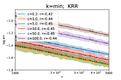
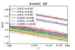
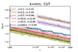
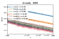
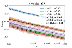
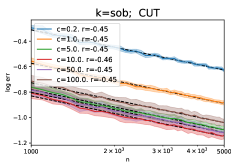
Figure 2: Error decay curves of two kinds of RKHSs and three kinds of spectral algorithms with different choices of $c$. Both axes are logarithmic.

References

- Adams (1975) R. Adams. Sobolev Spaces. Adams. Pure and applied mathematics. Academic Press, 1975. URL https://books.google.co.uk/books?id=JxzpSAAACAAJ.
- Adams and Fournier (2003) R. A. Adams and J. J. Fournier. Sobolev Spaces. Elsevier, 2003.
- Bach (2017) F. Bach. Breaking the curse of dimensionality with convex neural networks. The Journal of Machine Learning Research, 18(1):629–681, 2017.
- Bauer et al. (2007) F. Bauer, S. Pereverzyev, and L. Rosasco. On regularization algorithms in learning theory. Journal of complexity, 23(1):52–72, 2007.
- Beaglehole et al. (2022) D. Beaglehole, M. Belkin, and P. Pandit. Kernel ridgeless regression is inconsistent in low dimensions, June 2022.
- Blanchard and Mücke (2018) G. Blanchard and N. Mücke. Optimal rates for regularization of statistical inverse learning problems. Foundations of Computational Mathematics, 18:971–1013, 2018.
- Bordelon et al. (2020) B. Bordelon, A. Canatar, and C. Pehlevan. Spectrum dependent learning curves in kernel regression and wide neural networks. In ICML, 2020.
- Caponnetto (2006) A. Caponnetto. Optimal rates for regularization operators in learning theory. Technical report, MASSACHUSETTS INST OF TECH CAMBRIDGE COMPUTER SCIENCE AND ARTIFICIAL …, 2006.
- Caponnetto and de Vito (2007) A. Caponnetto and E. de Vito. Optimal rates for the regularized least-squares algorithm. Foundations of Computational Mathematics, 7:331–368, 2007.
- Celisse and Wahl (2020) A. Celisse and M. Wahl. Analyzing the discrepancy principle for kernelized spectral filter learning algorithms. J. Mach. Learn. Res., 22:76:1–76:59, 2020.
- Cho and Saul (2009) Y. Cho and L. Saul. Kernel methods for deep learning. In Y. Bengio, D. Schuurmans, J. Lafferty, C. Williams, and A. Culotta, editors, Advances in Neural Information Processing Systems, volume 22. Curran Associates, Inc., 2009.
- Cucker and Smale (2001) F. Cucker and S. Smale. On the mathematical foundations of learning. Bulletin of the American Mathematical Society, 39:1–49, 2001.
- Cui et al. (2021) H. Cui, B. Loureiro, F. Krzakala, and L. Zdeborov’a. Generalization error rates in kernel regression: The crossover from the noiseless to noisy regime. In NeurIPS, 2021.
- Dai and Xu (2013) F. Dai and Y. Xu. Approximation Theory and Harmonic Analysis on Spheres and Balls. Springer Monographs in Mathematics. Springer New York, New York, NY, 2013. ISBN 978-1-4614-6659-8 978-1-4614-6660-4. doi: 10.1007/978-1-4614-6660-4.
- Dicker et al. (2017) L. Dicker, D. P. Foster, and D. J. Hsu. Kernel ridge vs. principal component regression: Minimax bounds and the qualification of regularization operators. Electronic Journal of Statistics, 11:1022–1047, 2017.