A Strong Duality Result for Constrained POMDPs with Multiple Cooperative Agents

Abstract

The work studies the problem of decentralized constrained POMDPs in a team-setting where multiple non-strategic agents have asymmetric information. Using an extension of Sion’s Minimax theorem for functions with positive infinity and results on weak-convergence of measures, strong duality is established for the setting of infinite-horizon expected total discounted costs when the observations lie in a countable space, the actions are chosen from a finite space, the constraint costs are bounded, and the objective cost is bounded from below.

I Introduction

Single-Agent Markov Decision Processes (SA-MDPs) [1] and Single-Agent Partially Observable Markov Decision Processes (SA-POMDPs) [2] have long served as the basic building-blocks in the study of sequential decision-making. An SA-MDP is an abstraction in which an agent sequentially interacts with a fully-observable Markovian environment to solve a multi-period optimization problem; in contrast, in SA-POMDP, the agent only gets to observe a noisy or incomplete version of the environment. In 1957, Bellman proposed dynamic-programming as an approach to solve SA-MDPs [1, 3]. This combined with the characterization of SA-POMDP into an equivalent SA-MDP [4, 5, 6] (in which the agent maintains a belief about the environment’s true state) made it possible to extend dynamic-programming results to SA-POMDPs. Reinforcement learning [7] based algorithmic frameworks ([8, 9, 10, 11, 12, 13] to name a few) use data-driven dynamic-programming approaches to solve such single-agent sequential decision-making problems when the environment is unknown.

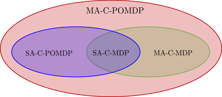
Figure 1: Relationships between Models of Cooperative Sequential Decision-Making under Constraints.

In many engineering systems, there are multiple decision-makers that collectively solve a sequential decision-making problem but with safety constraints: e.g., a team of robots performing a joint task, a fleet of automated cars navigating a city, multiple traffic-light controllers in a city, etc. Bandwidth constrained communications and communication delays in such systems lead to a decentralized team problem with information asymmetry. In this work, we study a fairly general abstraction of such systems, namely that of a cooperative multi-agent constrained POMDP, hereon referred to MA-C-POMDP. The special cases of MA-C-POMDP when there are no constraints, when there is only one agent, or when the environment is fully observable to each agent are referred to as MA-POMDP, SA-C-POMDP, and MA-C-MDP, respectively. The relationships among these models are shown in Figure 1.

I-A Related Work

I-A1 Single-Agent Settings

Prior work on planning and learning under constraints has primarily focused on single-agent constrained MDP (SA-C-MDP) where unlike in SA-MDPs, the agent solves a constrained optimization problem. For this setup, a number of fundamental results from the planning perspective have been derived – for instance, [15, 16, 17, 18, 19, 20, 21]; see [22] for details of the convex-analytic approach for SA-C-MDPs. These aforementioned results have led to the development of many algorithms in the learning setting: see [23, 24, 25, 26, 27, 28, 29]. Unlike SA-C-MDPs, rigorous results for SA-C-POMDPs are limited; few works for reference include [30, 31, 32, 33].

I-A2 Multi-Agent Settings

Challenges arising from the combination of partial observability of the environment and information-asymmetry have led to difficulties in developing general solutions to MA-POMDPs: e.g., solving a finite-horizon MA-POMDP with more than two agents is known to be NEXP-complete [34]. Nevertheless, conceptual approaches exist to establish solution methodologies and structural properties to (finite-horizon) MA-POMDPs namely: i) the person-by-person approach [35]; ii) the designer’s approach [36]; and iii) the common-information (CI) approach [37, 38]. Using a fictitious coordinator that only uses the common information to take actions, the CI approach allows for the transformation of the problem to a SA-POMDP which can be used to solve for an optimal control. The CI approach has also led to the development of a multi-agent reinforcement learning (MARL) framework [39] where agents learn good compressions of common and private information that can suffice for approximate optimality. On the empirical front, a few worth-mentioning works include [40, 41, 42, 43]. Finally, we note that work on MA-C-POMDPs is non-existent.

I-B Contribution

For MA-C-POMDPs, the technical challenges increase even more because restriction of the search space to deterministic policy-profiles is no longer an option. Therefore, the coordinator in the equivalent SA-C-POMDP has an uncountable prescription space, which leads to an uncountable state-space in its equivalent SA-C-MDP. This is an issue because most fundamental results in the theory of SA-C-MDPs (largely based on occupation-measures) rely heavily on the state-space being countably-infinite; see [22]. Due to these reasons, the study of MA-C-POMDPs calls for a new methodology – one which avoids this transformation and directly studies the decentralized problem. Our work takes the first steps in this direction and presents a rigorous approach for MA-C-POMDPs which is based on structural characterization of the set of behavioral policies and their performance measures, and using measure theoretic results. The main result in this paper, namely Theorem 1, establishes strong duality for MA-C-POMDPs, thus providing a firm theoretical basis for (future) development of primal-dual type planning and learning algorithms.

I-C Organization

The rest of the paper is organized as follows. Mathematical formulation of cooperative MA-C-POMDP is introduced in Section II. Strong duality results are then derived in Section III with details deferred to Appendices A, B, and C. Finally, concluding remarks are given in Section C.

I-D Notation

Before we present the model, we highlight the key notation in this paper.

• The sets of integers and positive integers are respectively denoted by $\mathbb{Z}$ and $\mathbb{N}$. For integers $a$ and $b$, $[a,b]_{\mathbb{Z}}$ represents the set $\{a,a+1,\dots,b\}$ if $a\leq b$ and $\emptyset$ otherwise. The notations [a] and $[a,\infty]_{\mathbb{Z}}$ are used as shorthands for $[1,a]_{\mathbb{Z}}$ and $\{a,a+1,\dots\}$, respectively.

• For integers $a\leq b$ and $c\leq d$, and a quantity of interest $q$, $q^{(a:b)}$ is a shorthand for the vector $\left(q^{(a)},q^{(a+1)},\dots,q^{(b)}\right)$ while $q_{c:d}$ is a shorthand for the vector $\left(q_{c},q_{c+1},\dots,q_{d}\right)$. The combined notation $q_{a:b}^{(c:d)}$ is a shorthand for the vector $(q_{i}^{(j)}:i\in[a,b]_{\mathbb{Z}},j\in[c,d]_{\mathbb{Z}})$. The infinite tuples $\left(q^{(a)},q^{(a+1)},\dots,\right)$ and $\left(q_{c},q_{c+1},\dots,\right)$ are respectively denoted by $q^{(a:\infty)}$ and $q_{c:\infty}$.

• For two real-valued vectors $v_{1}$ and $v_{2}$, the inequalitie $v_{1}\leq v_{2}$ and $v_{1}<v_{2}$ are meant to be element-wise inequalities.

• Probability and expectation operators are denoted by $\mathbb{P}$ and $\mathbb{E}$, respectively. Random variables are denoted by upper-case letters and their realizations by the corresponding lower-case letters. At times, we also use the shorthand $\mathbb{E}\left[\cdot|x\right]\overset{\Delta}{=}\mathbb{E}\left[\cdot|X=x\right]$ and $\mathbb{P}\left(y|x\right)\overset{\Delta}{=}\mathbb{P}\left(Y=y|X=x\right)$ for conditional quantities.

• Topological spaces are denoted by upper-case calligraphic letters. For a topological-space $\mathcal{W}$, $\mathcal{B}\left(\mathcal{W}\right)$ denotes the Borel $\sigma$-algebra, measurability is determined with respect to $\mathcal{B}\left(\mathcal{W}\right)$, and $M_{1}\left(\mathcal{W}\right)$ denotes the set of all probability measures on $\mathcal{B}\left(\mathcal{W}\right)$ endowed with the topology of weak convergence. Also, unless stated otherwise, “measure” means a non-negative measure.

• Unless otherwise stated, if a set $\mathcal{W}$ is countable, as a topological space it will be assumed to have the discrete topology. Therefore, the corresponding Borel $\sigma$-algebra $\mathcal{B}\left(\mathcal{W}\right)$ will be the power-set $2^{\mathcal{W}}$.

• Unless stated otherwise, the product of a collection of topological spaces will be assumed to have the product topology.

• The notation in Appendices B and C is exclusive and should be read independent of the rest of the manuscript.

II Model

Let $\left(N,\mathcal{S},\mathcal{O},\mathcal{A},\mathcal{P}_{tr},\left(c,d\right),P_{1},\mathcal{U},\alpha\right)$ denote a (cooperative) MA-C-POMDP with $N$ agents, state space $\mathcal{S}$, joint-observation-space $\mathcal{O}$, action-space $\mathcal{A}$, transition-law $\mathcal{P}_{tr}$, immediate-cost functions $c$ and $d$, (fixed) initial distribution $P_{1}$, space of decentralized policy-profiles $\mathcal{U}$, and discount factor $\alpha\in\left(0,1\right)$. The decision problem (to be detailed later on) has the following attributes and notations.

1. State Process: The state-space $\mathcal{S}$ is some topological space with a Borel $\sigma$-algebra $\mathcal{B}\left(\mathcal{S}\right)$. The state-process is denoted by $\left\{S_{t}\right\}_{t=1}^{\infty}$.

2. Joint-Observation Process: The joint-observation space $\mathcal{O}$ is a countable discrete space of the form $\mathcal{O}=\prod_{n=0}^{N}\mathcal{O}^{(n)}$, where $\mathcal{O}^{(0)}$ denotes the common observation space of all agents and $\mathcal{O}^{(n)}$ denotes the private observation space of agent $n\in[N]$. The joint-observation process is denoted by $\left\{O_{t}\right\}_{t=1}^{\infty}$ where $O_{t}=O_{t}^{(0:N)}$ and is such that at each time $t$, agent $n\in[N]$ observes $O_{t}^{(0)}$ and $O_{t}^{(n)}$ only.

3. Joint-Action Process: The joint-action space $\mathcal{A}$ is a finite discrete space of the form $\mathcal{A}=\prod_{n=1}^{N}\mathcal{A}^{(n)}$, where $\mathcal{A}^{(n)}$ denotes the action space of agent $n\in[N]$. The joint-action process is denoted by $\left\{A_{t}\right\}_{t=1}^{\infty}$ where $A_{t}=A_{t}^{(1:N)}$ and $A_{t}^{(n)}$ denotes the action of agent $n$ at time $t$. Since all $\mathcal{A}^{(n)}$’s and $\mathcal{A}$ are finite, they are all compact metric spaces.

4. Transition-law: At time $t\in\mathbb{N}$, given the current state $S_{t}$ and current joint-action $A_{t}$, the next state $S_{t+1}$ and the next joint-observation $O_{t+1}$ are determined in a time-homogeneous manner independent of all previous states, all previous and current joint-observations, and all previous joint-actions. The transition-law is given by

   $$\mathcal{P}_{tr}\overset{\Delta}{=}\left\{P_{saBo}:s\in\mathcal{S},a\in\mathcal{A},B\in\mathcal{B}\left(\mathcal{S}\right),o\in\mathcal{O}\right\},$$ (1)

   where for all $t\in\mathbb{N}$,

   $$\begin{split}&\mathbb{P}\left(S_{t+1}\in B,O_{t+1}=o|S_{1:t-1}=s_{1:t-1},\right.\\ &\hskip 12.5pt\left.O_{1:t}=o_{1:t},A_{1:t-1}=a_{1:t-1},S_{t}=s,A_{t}=a\right)\\ &\hskip 10.0pt=\mathbb{P}\left(S_{t+1}\in B,O_{t+1}=o|S_{t}=s,A_{t}=a\right)\\ &\hskip 10.0pt\overset{\Delta}{=}P_{saBo}.\end{split}$$ (2)

5. Immediate-costs: The immediate cost $c:\mathcal{S}\times\mathcal{A}\mapsto\mathbb{R}$ is a real-valued function whose expected discounted aggregate (to be defined later) we would like to minimize. On the other hand, the immediate cost $d:\mathcal{S}\times\mathcal{A}\mapsto\mathbb{R}^{K}$ is $\mathbb{R}^{K}$-valued function whose expected discounted aggregate we would like to keep within a specified threshold. For these reasons, we call $c$ and $d$ as the objective and constraint costs respectively. We shall make use of the following assumption on immediate-costs in Theorem 1.

   Assumption 1.

   The immediate objective cost is bounded from below and the immediate constraint costs are bounded, i.e., there exist $\underline{c}\in\mathbb{R}$ and $\underline{d},\overline{d}\in\mathbb{R}^{K}$ such that

   $$\underline{c}\leq c(\cdot,\cdot)\text{ and }\underline{d}\leq d(\cdot,\cdot)\leq\overline{d}.$$ (3)

   Let $\underaccent{\bar}{\bar{d}}=\|\underline{d}\|_{\infty}\vee\|\overline{d}\|_{\infty}$ so that $\|d(\cdot,\cdot)\|_{\infty}\leq\underaccent{\bar}{\bar{d}}<\infty$.

6. Initial Distribution: $P_{1}$ is a (fixed) probability measure for the initial state and initial joint-observation, i.e., $P_{1}\in M_{1}\left(\mathcal{S}\times\mathcal{O}\right)$ and

   $$\begin{split}P_{1}\left(B,o\right)&\overset{\Delta}{=}\mathbb{P}\left(S_{1}\in B,O_{1}=o\right).\end{split}$$ (4)

7. Space of Policy-Profiles: For time $t\in\mathbb{N}$, the common history of all agents is defined as all the common observations received thus far, i.e., $H_{t}^{(0)}\overset{\Delta}{=}\left(O_{1:t}^{(0)}\right)$. Similarly, the private history of agent $n$ at time $t$ is defined as all observations received and all the actions taken by the agent thus far (except for those that are part of the common information), i.e.,

   $$\begin{split}H_{1}^{(n)}&\overset{\Delta}{=}O_{1}^{(n)}\setminus O_{1}^{(0)},\text{ and}\\ H_{t}^{(n)}&\overset{\Delta}{=}\left(H_{t-1}^{(n)},(A_{t-1}^{(n)},O_{t}^{(n)})\setminus O_{t}^{(0)}\right)\ \forall t\in[2,\infty]_{\mathbb{Z}}.\end{split}$$ (5)

   Finally, the joint history at time $t$ is defined as the tuple of the common history and all the private histories at time $t$, i.e., $H_{t}\overset{\Delta}{=}H_{t}^{(0:n)}$.

   With the above setup, we define a (decentralized) behavioral policy-profile $u$ as a tuple $u^{(1:N)}\in\mathcal{U}\overset{\Delta}{=}\prod_{n=1}^{N}\mathcal{U}^{(n)}$ where $u^{(n)}$ denotes some behavioral policy used by agent $n$, i.e., $u^{(n)}$ itself is a tuple of the form $u_{1:\infty}^{(n)}$ where $u_{t}^{(n)}$ maps $\mathcal{H}_{t}^{(0)}\times\mathcal{H}_{t}^{(n)}$ to $M_{1}\left(\mathcal{A}^{(n)}\right)$, and where agent $n$ uses the distribution $u_{t}^{(n)}(H_{t}^{(0)},H_{t}^{(n)})$ to choose its action $A_{t}^{(n)}$. We pause to emphasize that at any time $t$, each agent randomizes over its action-set independently of all other agents (no common randomness). Thus, given a joint-history $h_{t}\in\mathcal{H}_{t}$ at time $t$, the probability that joint-action $a_{t}\in\mathcal{A}$ is taken is given by

   $$u_{t}\left(a_{t}|h_{t}\right) \overset{\Delta}{=}\prod_{n=1}^{N}u_{t}^{(n)}\left(h_{t}^{(0)},h_{t}^{(n)}\right)\left(a_{t}^{(n)}\right)$$

   $$=\prod_{n=1}^{N}u_{t}^{(n)}\left(a_{t}^{(n)}\big{|}h_{t}^{(0)},h_{t}^{(n)}\right).$$ (6)

   Remark 1.

   With Assumption 1, the expectations $\mathbb{E}_{P_{1}}\left[d\left(S_{t},A_{t}\right)\mid H_{t}=h_{t},A_{t}=a_{t}\right]$ are (element-wise) finite.

8. Optimization Problem: Let $\mathbb{P}^{\left(u\right)}_{P_{1}}$ be the probability measure corresponding to policy-profile $u\in\mathcal{U}$ and initial-distribution $P_{1}$, and let $\mathbb{E}^{\left(u\right)}_{P_{1}}$ denote the corresponding expectation operator. We define infinite-horizon expected total discounted costs $C:\mathcal{U}\rightarrow\mathbb{R}\cup\{\infty\}$ and $D:\mathcal{U}\rightarrow\mathbb{R}^{K}$ as

   $$C\left(u\right)=C^{(P_{1},\alpha)}\left(u\right) \overset{\Delta}{=}\mathbb{E}^{\left(u\right)}_{P_{1}}\left[\sum_{t=1}^{\infty}\alpha^{t-1}c\left(S_{t},A_{t}\right)\right],$$ (7)

   $$\text{and}\ D\left(u\right)=D^{(P_{1},\alpha)}\left(u\right) \overset{\Delta}{=}\mathbb{E}^{\left(u\right)}_{P_{1}}\left[\sum_{t=1}^{\infty}\alpha^{t-1}d\left(S_{t},A_{t}\right)\right].$$ (8)

   Remark 2.

   Assumption 1 ensures that $C\left(u\right)\in\mathbb{R}\cup\{\infty\}$, and $D\left(u\right)\in\mathbb{R}^{K}$ with (absolute) bound $\underaccent{\bar}{\bar{d}}/(1-\alpha)$.

   The decision process proceeds as follows: i) At each time $t\in\mathbb{N}$, the current state $S_{t}$ and observations $O_{t}$ are generated; ii) Each agent $n\in[N]$ chooses an action $a^{(n)}\in\mathcal{A}^{(n)}$ based on $H_{t}^{(0)},H_{t}^{(n)}$; iii) the immediate-costs $c\left(S_{t},A_{t}\right),d\left(S_{t},A_{t}\right)$ are incurred; iv) The system moves to the next state and observations according to the transition-law $\mathcal{P}_{tr}$. Under these rules, the goal of the agents is to work cooperatively to solve the following constrained optimization problem.

   $$\begin{split}&\text{minimize }C\left(u\right)\\ &\text{subject to }u\in\mathcal{U}\text{ and }D\left(u\right)\leq\overline{D}.\end{split}\Bigg{\}}$$ (MA-C-POMDP)

   Here, $\overline{D}$ is a fixed $K$-dimensional real-valued vector. We refer to the solution of (MA-C-POMDP) as its optimal value and denote it by $\underline{C}=\underline{C}^{(P_{1},\alpha)}$. In particular, if the set of feasible policy-profiles is empty, we set $\underline{C}$ to $\infty$ and with slight abuse of terminology will consider any policy-profile in $\mathcal{U}$ to be optimal.

   The following assumption about feasibility of (MA-C-POMDP) will be used in one of the parts of Theorem 1.

   Assumption 2 (Slater’s Condition).

   There exists a policy-profile $\overline{u}\in\mathcal{U}$ and $\zeta>0$ for which

   $$D\left(\overline{u}\right)\leq\overline{D}-\zeta 1.$$ (9)

III Characterization of Strong Duality

To solve (MA-C-POMDP), let us define the Lagrangian function $L:\mathcal{U}\times\mathcal{Y}\mapsto\mathbb{R}\cup\{\infty\}$ as follows.

$$L\left(u,\lambda\right) =L^{(P_{1},\alpha)}\left(u,\lambda\right)\overset{\Delta}{=}C\left(u\right)+\langle\lambda,D\left(u\right)-\overline{D}\rangle$$

$$=C\left(u\right)+\sum_{k=1}^{K}\lambda_{k}\left(D_{k}\left(u\right)-\overline{D}_{k}\right),$$ (10)

Here, $\mathcal{Y}\overset{\Delta}{=}\{\lambda\in\mathbb{R}^{K}:\lambda\geq 0\}$ is the set of tuples of $K$ non-negative real-numbers, each commonly known as a Lagrange-multiplier. Our main result shows that the the solution $\underline{C}$ satisfies

$$\underline{C} =\inf\limits_{u\in\mathcal{U}}\sup\limits_{\lambda\in\mathcal{Y}}L\left(u,\lambda\right),$$ (11)

and that the inf and sup can be interchanged, i.e.,

$$\underline{C} =\sup\limits_{\lambda\in\mathcal{Y}}\inf\limits_{u\in\mathcal{U}}L\left(u,\lambda\right).$$ (12)

Theorem 1 (Strong Duality).

Under Assumption 1, the following statements hold.

1. The optimal value satisfies

   $$\underline{C}=\inf\limits_{u\in\mathcal{U}}\sup\limits_{\lambda\in\mathcal{Y}}L\left(u,\lambda\right).$$ (13)

2. A policy-profile $u^{\star}\in\mathcal{U}$ is optimal if and only if $\underline{C}=\sup_{\lambda\in\mathcal{Y}}L\left(u^{\star},\lambda\right)$.

3. Strong duality holds for (MA-C-POMDP), i.e.,

   $$\underline{C} =\inf\limits_{u\in\mathcal{U}}\sup\limits_{\lambda\in\mathcal{Y}}L\left(u,\lambda\right)=\sup\limits_{\lambda\in\mathcal{Y}}\inf\limits_{u\in\mathcal{U}}L\left(u,\lambda\right).$$ (14)

   Moreover, there exists a $u^{\star}\in\mathcal{U}$ such that $\underline{C}=\sup_{\lambda\in\mathcal{Y}}L\left(u^{\star},\lambda\right)$ and $u^{\star}$ is optimal for (MA-C-POMDP). In particular, if Assumption 2 holds, then there also exists $\lambda^{\star}\in\mathcal{Y}$ such that the following saddle-point condition holds for all $(u,\lambda)\in\mathcal{U}\times\mathcal{Y}$,

   $$L\left(u^{\star},\lambda\right)\leq L\left(u^{\star},\lambda^{\star}\right)=\underline{C}\leq L\left(u,\lambda^{\star}\right).$$ (15)

   i.e., $u^{\star}$ minimizes $L\left(\cdot,\lambda^{\star}\right)$ and $\lambda^{\star}$ maximizes $L\left(u^{\star},\cdot\right)$. In addition to this, the primal dual pair $\left(u^{\star},\lambda^{\star}\right)$ satisfies the complementary-slackness condition:

   $$\langle\lambda^{\star},D\left(u^{\star}\right)-\overline{D}\rangle=0.$$ (16)

Proof.

1. If $u\in\mathcal{U}$ is feasible (i.e., it satisfies $D\left(u\right)\leq\overline{D}$), then the $\sup$ is obtained by choosing $\lambda=0$, so

   $$\sup_{\lambda\in\mathcal{Y}}L\left(u,\lambda\right) =C\left(u\right).$$ (17)

   If $u\in\mathcal{U}$ is not feasible, then

   $$\sup_{\lambda\in\mathcal{Y}}L\left(u,\lambda\right)=\infty.$$ (18)

   Indeed, suppose WLOG that the $k^{th}$ constraint is violated, i.e., $D_{k}\left(u\right)>\overline{D}_{k}$, then $\infty$ can be obtained by choosing $\lambda_{k}$ arbitrarily large and setting other $\lambda_{k}$’s to 0.

   From (17), (18), and our convention that $\underline{C}=\infty$ whenever the feasible-set is empty, it follows that

   $$\underline{C}=\inf\limits_{u\in\mathcal{U}}\sup\limits_{\lambda\in\mathcal{Y}}L\left(u,\lambda\right).$$ (19)

2. By our convention on the value of $\underline{C}$ (when there is no feasible policy-profile), $u^{\star}$ is optimal if and only if $C\left(u^{\star}\right)=\underline{C}$, i.e., $\sup_{\lambda\in\mathcal{Y}}L\left(u^{\star},\lambda\right)=\underline{C}$.

3. To establish strong duality, we use Proposition 11 which requires $\mathcal{U}$ and $\mathcal{Y}$ to be convex topological spaces (with $\mathcal{U}$ being compact also). It is clear that $\mathcal{Y}$ is convex and we can endow it with the usual subspace topology of $\mathbb{R}^{K}$. For $\mathcal{U}$ however, we need to endow it with a suitable topology in which it is compact and then also show that it is convex. To achieve compactness, we can use the finiteness of action-space $\mathcal{A}^{(n)}$ and the countability of observation-space $\mathcal{O}$ to associate $\mathcal{U}$ with a product of compact sets that are parameterized by (countable number of) all possible histories. Tychonoff’s theorem (see Proposition 4) then helps achieve compactness under the product topology. (Convexity comes trivially). Now, we make this idea precise. For $n\in[0,N]_{\mathbb{Z}}$, let $\mathcal{H}_{t}^{(n)}$ denote the set of all possible realizations of $H_{t}^{(n)}$. Then, by countability of observation and action spaces, the sets

   $$\begin{split}\mathcal{H}_{t}&\overset{\Delta}{=}\prod_{n=0}^{N}\mathcal{H}_{t}^{(n)},\\ \mathcal{H}^{(n)}&\overset{\Delta}{=}\bigcup_{t=1}^{\infty}\mathcal{H}_{t}^{(0)}\times\mathcal{H}_{t}^{(n)},\text{ and }\\ \mathcal{H}&\overset{\Delta}{=}\bigcup_{t=1}^{\infty}\mathcal{H}_{t},\end{split}$$ (20)

   are countable. Here, $\mathcal{H}_{t}$ is the set of all possible joint-histories at time $t$, $\mathcal{H}^{(n)}$ is the set of all possible histories of agent $n$, and $\mathcal{H}$ is the set of all possible joint-histories. With this in mind, one observes that $\mathcal{U}$ is in one-to-one correspondence with the set $\mathcal{X}_{\mathcal{U}}\overset{\Delta}{=}\prod_{n=1}^{N}\mathcal{X}_{\mathcal{U}^{(n)}}$, where

   $$\mathcal{X}_{\mathcal{U}^{(n)}}\overset{\Delta}{=}\prod_{h\in\mathcal{H}^{(n)}}M_{1}\left(\mathcal{A}^{(n)};h\right),$$ (21)

   where $M_{1}\left(\mathcal{A}^{(n)};h\right)$ is a copy of $M_{1}\left(\mathcal{A}^{(n)}\right)$ dedicated for agent-$n$’s history $h$. For example, a given policy $u$ would correspond to a point $x\in\mathcal{X}_{\mathcal{U}}$ such that $x_{n,\left(h_{t}^{(0)},h_{t}^{(n)}\right)}=u_{t}^{(n)}\left(\cdot|h_{t}^{(0)},h_{t}^{(n)}\right)$, and similarly, vice versa.

   Now, given $\mathcal{A}^{(n)}$ is a complete separable (compact) metric space, by Prokhorov’s Theorem (see Proposition 6), each $M_{1}\left(\mathcal{A}^{(n)};h\right)$ is a compact (and convex) metric space (with the topology of weak-convergence). Therefore, endowing $\mathcal{X}_{\mathcal{U}^{(n)}}$ and $\mathcal{X}_{\mathcal{U}}$ with the product topology makes each a compact (and convex) metric space via Tychonoff’s theorem (see Proposition 4), which is also metrizable (via Proposition 5). Given $\mathcal{U}^{(n)}$ and $\mathcal{U}$ are respectively identifiable with $\mathcal{X}_{\mathcal{U}^{(n)}}$ and $\mathcal{X}_{\mathcal{U}}$, from now onwards, we assume that $\mathcal{U}^{(n)}$ and $\mathcal{U}$ have the same topology as that of $\mathcal{X}_{\mathcal{U}^{(n)}}$ and $\mathcal{X}_{\mathcal{U}}$ respectively. Thus, henceforth, we will consider $C$, $D_{k}$, and $L$ as functions on topological spaces. Furthermore, since we have been able to show $\mathcal{U}^{(n)}$’s and $\mathcal{U}$ as compact metric spaces (hence complete and separable as well), we can also define $\mathcal{B}\left(\mathcal{U}^{(n)}\right)$, $\mathcal{B}\left(\mathcal{U}\right)=\otimes_{n=1}^{N}\mathcal{B}\left(\mathcal{U}^{(n)}\right)$, $M_{1}\left(\mathcal{U}^{(n)}\right)$, and $M_{1}\left(\mathcal{U}\right)$, where the last two are compact (and convex) metrizable spaces by Prokhorov’s theorem (see Proposition 6).

   To establish part (c), it will be helpful to work with (decentralized) mixtures of behavioral policy-profiles – wherein each agent first uses a measure $\mu^{(n)}\in M_{1}\left(\mathcal{U}^{(n)}\right)$ to choose its policy-profile $u^{(n)}$ and then proceeds with it from time 1 onward. We denote this enlarged space by $\mathcal{U}_{\mathrm{mixed}}\overset{\Delta}{=}\prod_{n=1}^{N}M_{1}\left(\mathcal{U}^{(n)}\right)$, whose typical element, denoted by $\mu\overset{\Delta}{=}\mathop{\operatorname{\times}}_{n=1}^{N}\mu^{(n)}$, is a factorized measure on $\mathcal{U}$, i.e., $\mu^{(n)}\in M_{1}\left(\mathcal{U}^{(n)}\right)$. Now, we can extend the definition of the Lagrangian function to $\mathcal{U}_{\mathrm{mixed}}$ by defining $\overline{L}:\mathcal{U}_{\mathrm{mixed}}\times\mathcal{Y}\rightarrow\mathbb{R}\cup\{\infty\}$, where

   $$\overline{L}\left(\mu,\lambda\right) =\overline{L}^{(P_{1},\alpha)}\left(\mu,\lambda\right)\overset{\Delta}{=}\mathbb{E}^{(\mu)}\left[L\left(u,\lambda\right)\right],$$ (22)

   In Lemma 4, it is shown that any $\mu\in\mathcal{U}_{\mathrm{mixed}}$ can be replicated by a behavioral policy-policy $u\in\mathcal{U}$. Corollary 4.1 then shows that

   $$\begin{split}\inf\limits_{u\in\mathcal{U}}\sup\limits_{\lambda\in\mathcal{Y}}L\left(u,\lambda\right)&=\inf\limits_{\mu\in\mathcal{U}_{\mathrm{mixed}}}\sup\limits_{\lambda\in\mathcal{Y}}\overline{L}\left(\mu,\lambda\right),\text{ and }\\ \sup\limits_{\lambda\in\mathcal{Y}}\inf\limits_{u\in\mathcal{U}}L\left(u,\lambda\right)&=\sup\limits_{\lambda\in\mathcal{Y}}\inf\limits_{u\in\mathcal{U}_{\mathrm{mixed}}}\overline{L}\left(\mu,\lambda\right).\end{split}$$ (23)

   In light of (23), it suffices to prove part (c) for $\overline{L}$. By definition, $\overline{L}$ is affine and thus trivially concave in $\lambda$. Proposition 8 implies that $\overline{L}$ is convex in $\mu$ and Lemma 2 shows that $\overline{L}$ is lower semi-continuous in $\mu$. From Proposition 11, it then follows that

   $$\inf\limits_{u\in\mathcal{U}_{\mathrm{mixed}}}\sup\limits_{\lambda\in\mathcal{Y}}\overline{L}\left(u,\lambda\right)=\sup\limits_{\lambda\in\mathcal{Y}}\inf\limits_{\mathcal{U}_{\mathrm{mixed}}}\overline{L}\left(u,\lambda\right),$$

   and that there exists $\mu^{\star}\in\mathcal{U}_{\mathrm{mixed}}$ such that

   $$\sup_{\lambda\in\mathcal{Y}}L\left(\mu^{\star},\lambda\right)=\inf\limits_{u\in\mathcal{U}_{\mathrm{mixed}}}\sup\limits_{\lambda\in\mathcal{Y}}\overline{L}\left(u,\lambda\right).$$

   The optimality of $\mu^{\star}$ is implied by parts (b) and (a) and the final claim (using Assumption 2) follows from Lagrange-multiplier theory.

This concludes the proof. ∎

Lemma 2 (Lower Semi-Continuity of $\overline{L}$ on $\mathcal{U}_{\mathrm{mixed}}$).

Under Assumption 1, $\overline{L}$ is lower semi-continuous on $\mathcal{U}_{\mathrm{mixed}}$.

Proof.

Fix $\lambda\in\mathcal{Y}$ and $\mu\in\mathcal{U}_{\mathrm{mixed}}$. Let $\left\{\mu_{i}\right\}_{i=1}^{\infty}$ be a sequence of (factorized) measures that converges (weakly) to $\mu$ in $\mathcal{U}_{\mathrm{mixed}}\subseteq M_{1}\left(\mathcal{U}\right)$. Since $\mathcal{U}_{\mathrm{mixed}}$ is closed in $M_{1}\left(\mathcal{U}\right)$, $\left\{\mu_{i}\right\}_{i=1}^{\infty}$ also converges (weakly) to $\mu$ in $M_{1}\left(\mathcal{U}\right)$. We want to show

$$\liminf_{i\rightarrow\infty}\mathbb{E}^{\left(\mu_{i}\right)}_{P_{1}}\left[L\left(u,\lambda\right)\right]\geq\mathbb{E}^{\left(\mu\right)}_{P_{1}}\left[L\left(u,\lambda\right)\right].$$

By Lemma 3, $L$ is (point-wise) lower semi-continuous on $\mathcal{U}$. Therefore, Proposition 9 applies on $M_{1}\left(\mathcal{U}\right)$ and the above inequality follows. ∎

Lemma 3 (Lower Semi-Continuity of $L$ on $\mathcal{U}$).

Under Assumption 1, the functions $C$ and $D_{k}$’s are lower semi-continuous on $\mathcal{U}$. Hence, $L$ is lower semi-continuous on $\mathcal{U}$.

Proof.

We will prove the statement for $C$. The proof of lower semi-continuity of $D_{k}$’s is similar. For brevity, let

$$p\left(u,t,h_{t},a_{t}\right) =p_{P_{1}}\left(u,t,h_{t},a_{t}\right)\overset{\Delta}{=}\mathbb{P}^{\left(u\right)}_{P_{1}}\left(H_{t}=h_{t},A_{t}=a_{t}\right),$$

$$W\left(u,t,h_{t},a_{t}\right) =W_{P_{1}}\left(u,t,h_{t},a_{t}\right)$$

$$\overset{\Delta}{=}p\left(u,t,h_{t},a_{t}\right)\mathbb{E}_{P_{1}}\left[c\left(S_{t},A_{t}\right)|H_{t}=h_{t},A_{t}=a_{t}\right].$$

Then,

$$C\left(u\right) =\mathbb{E}^{\left(u\right)}_{P_{1}}\left[\sum_{t=1}^{\infty}\alpha^{t-1}c(S_{t},A_{t})\right]$$

$$=\mathbb{E}^{\left(u\right)}_{P_{1}}\left[\sum_{t=1}^{\infty}\alpha^{t-1}\left(c(S_{t},A_{t})-\underline{c}\right)\right]+\sum_{t=1}^{\infty}\alpha^{t-1}\underline{c}$$

$$\stackrel{{\scriptstyle\textnormal{(a)}}}{{\mathstrut{=}}}\sum_{t=1}^{\infty}\alpha^{t-1}\mathbb{E}^{\left(u\right)}_{P_{1}}\left[c(S_{t},A_{t})-\underline{c}\right]+\sum_{t=1}^{\infty}\alpha^{t-1}\underline{c}$$

$$=\sum_{t=1}^{\infty}\alpha^{t-1}\mathbb{E}^{\left(u\right)}_{P_{1}}\left[c(S_{t},A_{t})\right]$$

$$\stackrel{{\scriptstyle\textnormal{(b)}}}{{\mathstrut{=}}}\sum_{t=1}^{\infty}\alpha^{t-1}\mathbb{E}^{\left(u\right)}_{P_{1}}\left[\mathbb{E}_{P_{1}}\left[c(S_{t},A_{t})\right]|H_{t},A_{t}\right]$$

$$=\sum_{t=1}^{\infty}\sum_{h_{t}\in\mathcal{H}_{t}}\sum_{a_{t}\in\mathcal{A}}\alpha^{t-1}W\left(u,t,h_{t},a_{t}\right).$$

Here, (III) follows from applying the Monotone-Convergence Theorem to the (increasing non-negative) sequence $\{\sum_{t=1}^{i}\alpha^{t-1}\left(c\left(S_{t},A_{t}\right)-\underline{c}\right)\}_{i=1}^{\infty}$ (see Proposition 1); and (III) uses the tower property of conditional expectation.

Let $\left\{{}^{i}u\right\}_{i=1}^{\infty}$ be a sequence in $\mathcal{U}$ that converges to $u$. By Fatou’s Lemma (see Proposition 3),

$$\liminf_{i\rightarrow\infty}C\left({}^{i}u\right)\geq\sum_{t=1}^{\infty}\sum_{h_{t}\in\mathcal{H}_{t}}\sum_{a_{t}\in\mathcal{A}}\alpha^{t-1}\liminf_{i\rightarrow\infty}W\left({}^{i}u,t,h_{t},a_{t}\right).$$ (24)

Following Lemma 5, $p\left({}^{i}u,t,h_{t},a_{t}\right)$ converges to $p\left(u,t,h_{t},a_{t}\right)$. Therefore,

$$\lim_{i\rightarrow\infty}W\left({}^{i}u,t,h_{t},a_{t}\right)=W\left(u,t,h_{t},a_{t}\right).$$ (25)

From (24) and (25), it follows that

$$\liminf_{i\rightarrow\infty}C\left({}^{i}u\right)\geq C\left(u\right),$$

which establishes the lower semi-continuity of $C\left(u\right)$. ∎

IV Conclusion

In this work, we studied a cooperative multi-agent constrained POMDP in the setting of infinite-horizon expected total discounted costs. We established strong-duality using an extension of Sion’s Minimax Theorem which required giving a suitable topology to the space of all possible policy-profiles and then establishing lower semi-continuity of the Lagrangian function. The strong duality result provides a firm theoretical footing for future work on developing primal-dual type planning and learning algorithms for MA-C-POMDPs.

Appendix A Intermediary Results for Theorem 1

Lemma 4 (Equivalence between Behavioral Policy-Profiles and their (decentralized) Mixtures).

Fix a (factorized) measure $\mu\in\mathcal{U}_{\mathrm{mixed}}$. Then there exists a behavioral policy-profile $\underline{u}=\underline{u}(\mu)\in\mathcal{U}$, such that for any $t\in\mathbb{N}$, $h_{t}\in\mathcal{H}_{t}$, and $a_{t}\in\mathcal{A}$,

$$p\left(\mu,t,h_{t},a_{t}\right)=p\left(u,t,h_{t},a_{t}\right),$$

where, for brevity and with slight abuse of notation,

$$p\left(\cdot,t,h_{t},a_{t}\right) =\mathbb{P}^{\left(\cdot\right)}_{P_{1}}\left(H_{t}=h_{t},A_{t}=a_{t}\right),\text{ and}$$

$$p\left(\cdot,t,h_{t}\right) =\mathbb{P}^{\left(\cdot\right)}_{P_{1}}\left(H_{t}=h_{t}\right).$$

Proof.

Define $\underline{u}=\underline{u}(\mu)\in\mathcal{U}$ such that

$$\underline{u}_{t}\left(a_{t}|h_{t}\ \right)=\prod_{n=1}^{N}\underline{u}_{t}^{(n)}\left(a_{t}^{(n)}|h_{t}^{(0)},h_{t}^{(n)}\right)$$

$$=\begin{cases}\frac{p\left(\mu,t,h_{t},a_{t}\right)}{p\left(\mu,t,h_{t}\right)},&\text{if }p\left(\mu,t,h_{t}\right)\neq 0,\\ \prod_{n=1}^{N}\frac{1}{|\mathcal{A}^{(n)}|},&\text{otherwise}.\end{cases}$$ (A.26)

To see that the above assignment is correct, we note that the right-hand-side of (A.26) is a fully-factorized function of $a_{t}^{(n)}$’s, as follows.

$$p\left(\mu,t,h,a\right)=\int_{U}\mu\left(du\right)\mathbb{P}^{\left(u\right)}_{P_{1}}\left(H_{t}=h_{t},A_{t}=a_{t}\right)$$

$$=\int_{\mathcal{U}}P_{1}\left(\mathcal{S},h_{1}\right)\prod_{t^{\prime}=2}^{t}\mathbb{P}_{P_{1}}\left(o_{t^{\prime}}|h_{t^{\prime}-1},a_{t^{\prime}-1}\right)$$

$$\hskip 10.0pt\times\prod_{n=1}^{N}\prod_{t^{\prime}=1}^{t}u_{t^{\prime}}^{(n)}\left(a_{t^{\prime}}^{(n)}|h_{t^{\prime}}^{(0)},h_{t^{\prime}}^{(n)}\right)\left(\left(\mathop{\operatorname{\times}}_{n=1}^{N}\mu^{(n)}\right)(du)\right)$$

$$=P_{1}\left(\mathcal{S},h_{1}\right)\prod_{t^{\prime}=1}^{t}\mathbb{P}_{P_{1}}\left(o_{t^{\prime}}|h_{t-1},a_{t^{\prime}-1}\right)$$

$$\hskip 10.0pt\times\prod_{n=1}^{N}\int_{\mathcal{U}^{(n)}}\prod_{t^{\prime}=1}^{t}u_{t^{\prime}}^{(n)}\left(a_{t^{\prime}}^{(n)}|h_{t^{\prime}}^{(0)},h_{t^{\prime}}^{(n)}\right)\mu^{(n)}\left(du^{(n)}\right),$$

where the last equality follows from Tonneli’s Theorem (see Proposition 2). We will now prove, by forward induction, that $\underline{u}$ and $\mu$ induce the same distribution on $\left(H_{t},A_{t}\right)$ for all $t\in\mathbb{N}$.

1. Base Case: For time $t=1$, let $o_{1}\in\mathcal{H}_{1}=\mathcal{O}$ and $a_{1}\in\mathcal{A}$. We have

   $$p\left(\mu,1,o_{1},a_{1}\right) =P_{1}\left(\mathcal{S},o_{1}\right)\int_{\mathcal{U}}\mu\left(du\right)u_{1}\left(a_{1}|o_{1}\right),$$

   and

   $$p\left(\underline{u},1,o_{1},a_{1}\right) =P_{1}\left(\mathcal{S},o_{1}\right)\underline{u}_{1}\left(a_{1}|o_{1}\right)$$

   $$=P_{1}\left(\mathcal{S},o_{1}\right)\frac{p\left(\mu,1,o_{1},a_{1}\right)}{p\left(\mu,1,o_{1}\right)}$$

   $$=p\left(\mu,1,o_{1},a_{1}\right),$$

   where the last equality follows from $p\left(\mu,1,o_{1}\right)=P_{1}\left(\mathcal{S},o_{1}\right)$.

2. Induction Step. Assuming that the statement is true for time $t$, we show that it is true for time $t+1$. Let $h_{t+1}=\left(o_{1:t+1},a_{1:t}\right)=\left(h_{t},a_{t},o_{t+1}\right)\in\mathcal{H}_{t+1}$ and $a_{t+1}\in\mathcal{A}$. We have

   $$p\left(\mu,t+1,h_{t+1}\right) =\int_{\mathcal{U}}\mu\left(du\right)\mathbb{P}^{\left(u\right)}_{P_{1}}\left(H_{t+1}=h_{t+1}\right)$$

   $$=\int_{\mathcal{U}}\mu\left(du\right)\mathbb{P}^{\left(u\right)}_{P_{1}}\left(H_{t+1}=h_{t+1}\right)$$

   $$=\int_{\mathcal{U}}\mu\left(du\right)\mathbb{P}^{\left(u\right)}_{P_{1}}\left(H_{t}=h_{t},A_{t}=a_{t},O_{t+1}=o_{t+1}\right)$$

   $$=\int_{\mathcal{U}}\mu\left(du\right)\mathbb{P}^{\left(u\right)}_{P_{1}}\left(H_{t}=h_{t},A_{t}=a_{t},\right)$$

   $$\times\mathbb{P}^{\left(u\right)}_{P_{1}}\left(O_{t+1}=o_{t+1}|H_{t}=h_{t},A_{t}=a_{t}\right)$$

   $$=\int_{\mathcal{U}}\mu\left(du\right)\mathbb{P}^{\left(u\right)}_{P_{1}}\left(H_{t}=h_{t},A_{t}=a_{t},\right)$$

   $$\times\mathbb{P}_{P_{1}}\left(O_{t+1}=o_{t+1}|H_{t}=h_{t},A_{t}=a_{t}\right)$$

   $$=p\left(\mu,t,h_{t},a_{t}\right)\mathbb{P}_{P_{1}}\left(O_{t+1}=o_{t+1}|H_{t}=h_{t},A_{t}=a_{t}\right)$$

   $$\stackrel{{\scriptstyle\textnormal{(c)}}}{{\mathstrut{=}}}p\left(\underline{u},t,h_{t},a_{t}\right)\mathbb{P}_{P_{1}}\left(O_{t+1}=o_{t+1}|H_{t}=h_{t},A_{t}=a_{t}\right)$$

   $$=p\left(\underline{u},t+1,h_{t+1}\right),$$

   where (2) uses the inductive hypothesis. The above work implies

   $$p\left(\underline{u},t+1,h_{t+1},a_{t+1}\right)$$

   $$=p\left(\underline{u},t+1,h_{t+1}\right)\cdot\ \underline{u}_{t+1}\left(a_{t+1}|h_{t+1}\right)$$

   $$=p\left(\mu,t+1,h_{t+1}\right)\frac{p\left(\mu,t+1,h_{t+1},a_{t+1}\right)}{p\left(\mu,t+1,h_{t+1}\right)}$$

   $$=p\left(\mu,t+1,h_{t+1},a_{t+1}\right).$$

This completes the proof. ∎

Corollary 4.1.

Fix $\lambda\in\mathcal{Y}$. For any $\mu\in\mathcal{U}_{\mathrm{mixed}}$, there exists $u=u(\mu)\in\mathcal{U}$ such that $L\left(u,\lambda\right)=\overline{L}\left(\mu,\lambda\right)$.

Proof.

One notes that $C\left(u\right)$ and $D\left(u\right)$ can be written as:

$$C\left(u\right) =\sum_{t=1}^{\infty}\alpha^{t-1}\mathbb{E}^{\left(\mu\right)}_{P_{1}}\left[\mathbb{E}_{P_{1}}\left[c\left(S_{t},A_{t}\right)\right]|H_{t},A_{t}\right],$$

$$D\left(u\right) =\sum_{t=1}^{\infty}\alpha^{t-1}\mathbb{E}^{\left(\mu\right)}_{P_{1}}\left[\mathbb{E}_{P_{1}}\left[d\left(S_{t},A_{t}\right)\right]|H_{t},A_{t}\right],$$

and the result follows. ∎

Lemma 5.

[Limit Probabilities for a converging sequence of policy-profiles] Let $\left\{{}^{i}u\right\}_{i=1}^{\infty}$ be a sequence in $\mathcal{U}$ that converges to $u$. Then, for any $t\in\mathbb{N}$, $h_{t}\in\mathcal{H}_{t}$, and $a_{t}\in\mathcal{A}$,

$$\lim_{i\rightarrow\infty}p\left({}^{i}u,t,h_{t},a_{t}\right)=p\left(u,t,h_{t},a_{t}\right),$$

where $p\left(\cdot,t,h_{t},a_{t}\right)=\mathbb{P}^{\left(\cdot\right)}_{P_{1}}\left(H_{t}=h_{t},A_{t}=a_{t}\right)$. In other words, for every $t\in\mathbb{N}$, the sequence of measures $\left\{p\left({}^{i}u,t,\cdot,\cdot\right)\right\}_{i=1}^{\infty}$ converges weakly to $p\left(u,t,\cdot,\cdot\right)$.

Proof.

Given that ${}^{i}u$ converges to $u$, by the definition of convergence in product topology, for every $n\in[N]$, ${}^{i}u_{t}^{(n)}(h_{t}^{(0)},h_{t}^{(n)})$ converges weakly to $u_{t}^{(n)}(h_{t}^{(0)},h_{t}^{(n)})$. Since $\mathcal{A}^{n}$ is finite, this means that for each $a^{(n)}\in\mathcal{A}^{(n)}$, ${}^{i}u_{t}^{(n)}(a^{(n)}|h_{t}^{(0)},h_{t}^{(n)})$ converges to $u_{t}^{(n)}(a^{(n)}|h_{t}^{(0)},h_{t}^{(n)})$, which further implies that for all $a\in\mathcal{A}$, ${}^{i}u_{t}(a|h_{t})$ converges to $u_{t}(a|h_{t})$. Now, we use forward induction to prove the statement.

1. Base Case: For time $t=1$, let $o_{1}\in\mathcal{H}_{1}=\mathcal{O}$ and $a_{1}\in\mathcal{A}$. We have

   $$p\left({}^{i}u,1,o_{1},a_{1}\right)=P_{1}\left(\mathcal{S},o\right)^{i}u_{1}\left(a_{1}|o_{1}\right)\rightarrow p\left(u,1,o_{1},a_{1}\right).$$

2. Induction Step: Assuming that the statement is true for time $t$, we show that it is true for time $t+1$. Let $h_{t+1}=\left(o_{1:t+1},a_{1:t}\right)=\left(h_{t},a_{t},o_{t+1}\right)\in\mathcal{H}_{t+1}$ and $a_{t+1}\in\mathcal{A}$. We have

   $$p\left({}^{i}u,t+1,h_{t+1},a_{t+1}\right)$$

   $$=p\left({}^{i}u,t,h_{t},a_{t}\right)^{i}u_{t+1}\left(a_{t+1}|h_{t+1}\right)$$

   $$\hskip 5.0pt\times\mathbb{P}_{P_{1}}\left(O_{t+1}=o_{t+1}|H_{t}=h_{t},A_{t}=a_{t}\right).$$

   By inductive hypothesis, $p\left({}^{i}u,t,h_{t},a_{t}\right)$ converges to $p\left(u,t,h_{t},a_{t}\right)$, and ${}^{i}u_{t}\left(a_{t+1}|h_{t+1}\right)$ converges to $u_{t}\left(a_{t+1}|h_{t+1}\right)$ by assumption. We conclude that $p\left({}^{i}u,t+1,h_{t+1},a_{t+1}\right)$ converges to $p\left(u,t+1,h_{t+1},a_{t+1}\right)$.

This completes the proof. ∎

Appendix B Helpful Facts and Results

Definition 1 (Lower Semi-continuous and Upper Semi-continuous Functions).

A function $f:\mathcal{X}\mapsto[-\infty,\infty]$ on a topological space $\mathcal{X}$ is called lower semi-continuous if for every point $x_{0}\in\mathcal{X}$,

$$\liminf\limits_{x\rightarrow x_{0}}f(x)\geq f(x_{0}).$$

We call $f$ as an upper semi-continuous function $-f$ is lower semi-continuous.

Proposition 1 (Monotone Convergence Theorem).

Let $\left(X,\mathcal{M},\mu\right)$ be a measure-space. Let $\left\{f_{i}\right\}_{i=1}^{\infty}$ be an increasing sequence of measurable functions which are uniformly bounded-from-below. Then,

$$\int_{X}\lim_{i\rightarrow\infty}f_{i}(x)\mu(dx)=\lim_{i\rightarrow\infty}\int_{X}f_{i}(x)\mu(dx).$$

Proposition 2 (Tonneli’s Theorem).

Let $f$ be a measurable function on the cartesian product of two $\sigma$-finite measure spaces $(X,\mathcal{M},\mu)$ and $(Y,\mathcal{N},\nu)$ which is bounded from below. Then,

$$\int_{X\times Y}f(x,y)(\mu\times\nu)(d(x,y))$$

$$\hskip 10.0pt=\int_{X}\left(\int_{Y}f(x,y)\nu(dy)\right)\mu(dx)$$

$$\hskip 10.0pt=\int_{Y}\left(\int_{X}f(x,y)\mu(dx)\right)\nu(dy).$$

Proposition 3 (Fatou’s Lemma).

Let $(X,\mathcal{M},\mu)$ be a measure-space and let $\{f_{i}\}_{i=1}^{\infty}$ be a sequence of measurable functions which are uniformly bounded from below. Then,

$$\liminf_{i\rightarrow\infty}\int f_{i}(x)\mu(dx)\geq\int\liminf_{i\rightarrow\infty}f_{i}(x)\mu(dx).$$

Proposition 4 (Tychonoff’s Theorem).

Product of countable number of compact spaces is compact under the product topology.

Proposition 5 (Metrizability of Product Topology on Countable Product of Metric Spaces).

Product of countable number of metric spaces, when endowed with the product topology, is metrizable.

Proposition 6 (Prokhorov’s Theorem).

Let $\left(\mathcal{X},d_{\mathcal{X}}\right)$ be a complete separable metric space with distance metric $d_{\mathcal{X}}$ and let $\mathcal{B}\left(\mathcal{X}\right)$ denote the Borel $\sigma$-algebra generated by $d_{\mathcal{X}}$. Let $M_{1}\left(\mathcal{X}\right)$ be the set of all probability measures on $\mathcal{B}\left(\mathcal{X}\right)$ and let $\tau$ denote the topology of weak-convergence on $M_{1}\left(\mathcal{X}\right)$. Then,

1. The topological space $\left(M_{1}\left(\mathcal{X}\right),\tau\right)$ is completely-metrizable. That is, there exists a complete metric $d_{M}$ on $M_{1}\left(\mathcal{X}\right)$ that induces the same topology as $\tau$.

2. An arbitrary collection $W\subseteq M_{1}\left(\mathcal{X}\right)$ of probability measures in $M_{1}\left(\mathcal{X}\right)$ is tight iff its closure in $\tau$ is compact (i.e., $W$ is precompact in $\tau$).

Proposition 7 (Hyperplane Separation Theorem).

Let $M$ be a non-empty convex subset of $\mathbb{R}^{n}$. If $x_{0}\in\mathbb{R}^{n}$ does not belong to $M$, there exists $\rho\in\mathbb{R}^{n}$ such that

$$\rho\neq 0\text{ and }\inf_{x\in M}\langle p,x\rangle\geq\langle p,x_{0}\rangle.$$

Proposition 8 (Integral of Bounded-from-Below function with respect to Convex Combination of Non-negative Measures).

Let $\left(X,\mathcal{M}\right)$ be a measure-space. Let $f:X\rightarrow\mathbb{R}\cup\{\infty\}$ be a measurable function that is bounded from below, and let $\mu,\nu$ be two non-negative measures on $\mathcal{M}$. Then, for any $\theta\in[0,1]$,

$$\int f(x)\left(\theta\mu+(1-\theta)\nu\right)(dx)$$

$$\hskip 10.0pt=\theta\int f(x)\mu(dx)+(1-\theta)\int f(x)\nu(dx).$$

Proposition 9 (Behavior of Integrals of a Bounded-from-Below and Lower Semi-Continuous Function).

Let $(\mathcal{X},d_{\mathcal{X}})$ be a complete separable metric space with distance metric $d_{\mathcal{X}}$ and let $\mathcal{B}\left(\mathcal{X}\right)$ denote the Borel $\sigma$-algebra generated by $d_{\mathcal{X}}$. Let $\left(M_{1}\left(\mathcal{X}\right),d_{M_{1}\left(\mathcal{X}\right)}\right)$ be the complete metric space of all probability measures on $\mathcal{B}\left(\mathcal{X}\right)$ with the topology of weak-convergence. Let $\mu\in M_{1}\left(\mathcal{X}\right)$ and let $f:\mathcal{X}\rightarrow\mathbb{R}\cup\left\{\infty\right\}$ be a function that is lower semi-continuous $\mu$-amost-everywhere and is bounded from below. Then, the function

$$H:M_{1}\left(\mathcal{X}\right)\mapsto\mathbb{R}\cup\left\{\infty\right\},\ H(\mu^{\prime})\overset{\Delta}{=}\int f(x)\mu^{\prime}(dx)$$

is lower semi-continuous at $\mu$. In particular, if $f$ is point-wise lower semi-continuous, then $H$ is also point-wise lower semi-continuous (on $M_{1}\left(\mathcal{X}\right)$).

Proof.

Define $f^{\prime}:\mathcal{X}\rightarrow\mathbb{R}\cup\{\infty\}$ as $f^{\prime}(x)\overset{\Delta}{=}f(x)\wedge\liminf_{y\rightarrow x}f(y)$. Then, $f^{\prime}$ minorizes $f$, is lower semi-continuous, and coincides with $f$ at $x$ if and only if $f$ is lower semi-continuous at $x$. Also, $f^{\prime}$ is bounded from below (since $f$ is). By Proposition 10, $f^{\prime}$ can be written as the point-wise limit of increasing sequence of uniformly bounded-from-below continuous functions from $\mathcal{X}$ into $\mathbb{R}\cup\{\infty\}$, say $\left\{g_{i}\right\}_{i=1}^{\infty}$, i.e., $f^{\prime}(x)=\lim_{i\rightarrow\infty}g_{i}(x)$. Then, for every $\mu^{\prime}\in M_{1}\left(\mathcal{X}\right)$,

$$\int f^{\prime}(x)\mu^{\prime}(dx)=\int\lim_{i\rightarrow\infty}g_{i}(x)\mu^{\prime}(dx)=\lim_{i\rightarrow\infty}\int g_{i}(x)\mu^{\prime}(dx),$$

where the last equality follows from the Montone Convergence Theorem (see Proposition 1). The above equality shows that the function $H^{\prime}:M_{1}\left(\mathcal{X}\right)\rightarrow\mathbb{R}\cup\{\infty\}$ such that $H^{\prime}(\mu^{\prime})=\int f^{\prime}(x)\mu^{\prime}(dx)$, is the point-wise limit of an increasing sequence of uniformly bounded-from-below continuous functions. Therefore, by Proposition 10, $H^{\prime}$ is lower semi-continuous. Now, if $f$ is lower semi-continuous $\mu$-almost-everywhere, then $f=f^{\prime}$ $\mu-$almost-everywhere. This gives,

$$H(\mu) =\int f(x)\mu(dx)$$

$$=\int f^{\prime}(x)\mu(dx)$$

$$\stackrel{{\scriptstyle\textnormal{(d)}}}{{\mathstrut{=}}}\liminf_{\mu^{\prime}\rightarrow\mu}H^{\prime}(\mu^{\prime})$$

$$\stackrel{{\scriptstyle\textnormal{(e)}}}{{\mathstrut{\leq}}}\liminf_{\mu^{\prime}\rightarrow\mu}H(\mu^{\prime}),$$

Here, (B) uses lower semi-continuity of $H^{\prime}$ and (B) follows from the fact that $H^{\prime}$ minorizes $H$ (since $f^{\prime}$ minorizes $f$). The inequality $H(\mu)\leq\liminf_{\mu^{\prime}\rightarrow\mu}H(\mu^{\prime})$ is the definition of lower semi-continuity at $\mu$. ∎

Proposition 10 (Equivalent Characterization of a Bounded-from-Below Lower Semi-Continuous Function).

Let $\left(\mathcal{X},d_{\mathcal{X}}\right)$ be a metric space. Then, a function $f:\mathcal{X}\rightarrow\mathbb{R}\cup\{\infty\}$ is a bounded-from-below lower semi-continuous function if and only if it can be written as the point-wise limit of an increasing sequence of uniformly bounded-from-below continuous functions from $\mathcal{X}$ into $\mathbb{R}\cup\{\infty\}$.

Proof.

Necessity: Define $f_{n}:\mathcal{X}\rightarrow\mathbb{R}\cup\{\infty\}$ as follows:

$$f_{n}\left(x\right) \overset{\Delta}{=}\inf_{y\in\mathcal{X}}\left\{f(y)+nd_{\mathcal{X}}\left(x,y\right)\right\}.$$

1. Increasing:

   $$f_{n+1}\left(x\right)=\inf_{y\in\mathcal{X}}\left\{f(y)+(n+1)d_{\mathcal{X}}\left(x,y\right)\right\}\geq f_{n}(x).$$

2. Uniformly Bounded-from-Below: Since $f_{n}\left(x\right)\geq\inf_{y\in\mathcal{X}}\left\{f(y)\right\}$ and $f$ is bounded-from-below, the functions $\left\{f_{n}\right\}_{n=1}^{\infty}$ are uniformly bounded-from-below.

3. Continuity: By triangle-inequality,

   $$f(y)+nd_{\mathcal{X}}\left(y,z\right)\leq f(y)+nd_{\mathcal{X}}\left(y,w\right)+nd_{\mathcal{X}}\left(w,z\right),$$

   and therefore, taking the infimum over $y$ on both sides gives $f_{n}\left(z\right)-f_{n}\left(w\right)\leq nd_{\mathcal{X}}\left(w,z\right)$. Similarly, we can get $f_{n}\left(w\right)-f_{n}\left(z\right)\leq nd_{\mathcal{X}}\left(w,z\right)$, and so

   $$|f_{n}\left(z\right)-f_{n}\left(w\right)|\leq nd_{\mathcal{X}}\left(w,z\right).$$

   The above relation shows that $f_{n}$ is Lipschitz and thus continuous.

4. Point-wise Convergence to $f$: Fix $x_{0}\in\mathcal{X}$ and $\epsilon>0$. We would like to show that there exists a positive integer $n^{\prime}=n^{\prime}(x_{0},\epsilon)$ such that, for all $n\geq n^{\prime}$, $|f_{n}\left(x_{0}\right)-f\left(x_{0}\right)|<\epsilon$. Since $f$ is lower semi-continuous at $x_{0}$, there exists $\delta=\delta(x_{0},\epsilon)>0$ such that

   $$d_{\mathcal{X}}\left(x_{0},y\right)<\delta\implies f(y)>f(x_{0})-\epsilon.$$ (B.27)

   Since $f$ is bounded-from-below (and $\delta>0$), there exists a positive integer $n^{\prime}=n^{\prime}(\delta(x_{0},\epsilon))$ such that

   $$d_{\mathcal{X}}\left(x_{0},y\right)\geq\delta$$

   $$\implies\forall\ n\geq n^{\prime},f(y)+nd_{\mathcal{X}}\left(x_{0},y\right)>f(x_{0})$$

   $$\implies\forall\ n\geq n^{\prime},\inf_{d_{\mathcal{X}}\left(x_{0},y\right)\geq\delta}\left\{f(y)+d_{\mathcal{X}}(x_{0},y)\right\}\geq f\left(x_{0}\right).$$

   So, for all $n\geq n^{\prime}$, we have

   $$f(x_{0})\geq f_{n}\left(x_{0}\right) =\inf_{d_{\mathcal{X}}\left(x_{0},y\right)\leq\delta}\left\{f(y)+nd_{\mathcal{X}}(x_{0},y)\right\}$$

   $$\geq\inf_{d_{\mathcal{X}}\left(x_{0},y\right)\leq\delta}\left\{f(y)\right\}$$

   $$\stackrel{{\scriptstyle\textnormal{(f)}}}{{\mathstrut{>}}}\inf_{d_{\mathcal{X}}\left(x_{0},y\right)\leq\delta}\left\{f(x_{0})-\epsilon\right\}$$

   $$=f(x_{0})-\epsilon.$$

   where (4) uses (B.27).

Sufficiency: Let $\left\{f_{n}\right\}_{n=1}^{\infty}$ be an increasing sequence of uniformly bounded-from-below continuous functions from $\mathcal{X}$ into $\mathbb{R}\cup\left\{\infty\right\}$. Since the sequence is monotonic, it has a point-wise-limit $f:\mathcal{X}\rightarrow\mathbb{R}\cup\left\{\infty\right\}$ which is bounded-from-below because all the functions in the sequence are uniformly bounded-from-below. We need to show that $f$ is lower semi-continuous.

Fix $x_{0}\in\mathcal{X}$ and $\epsilon>0$. We would like to show that there exists $\delta=\delta(x_{0},\epsilon)>0$ such that $d_{\mathcal{X}}\left(x_{0},y\right)<\delta\implies f(y)>f(x_{0})-\epsilon$. Since $\left\{f_{n}\right\}_{n=1}^{\infty}$ is increasing (and converges point-wise to $f$), there exists a positive integer $n^{\prime}=n^{\prime}(x_{0},\epsilon)$ such that, for all $n\geq n^{\prime}$, $f(x_{0})\geq f_{n}(x_{0})\geq f(x_{0})-\frac{\epsilon}{2}$. Since $f_{n^{\prime}}$ is lower semi-continuous, there exists $\delta=\delta(n^{\prime}(x_{0},\epsilon))>0$ such that $d_{\mathcal{X}}\left(x_{0},y\right)<\delta\implies f(y)\geq f_{n^{\prime}}(y)>f_{n^{\prime}}(x_{0})-\frac{\epsilon}{2}\geq f(x_{0})-\epsilon$. ∎

Appendix C A Minimax Theorem for Functions with Positive Infinity

Proposition 11 (A Minimax Theorem For Functions with Positive Infinity).

Let $\mathcal{X}$ and $\mathcal{Y}$ be convex topological spaces where $\mathcal{X}$ is also compact. Consider a function $f:\mathcal{X}\times\mathcal{Y}\rightarrow\mathbb{R}\cup\{\infty\}$ such that

1. for each $y\in\mathcal{Y}$, $f\left(\cdot,y\right)$ is convex and lower semi-continuous.

2. for each $x\in\mathcal{X}$, $f\left(x,\cdot\right)$ is concave.

3. If $f(x,y)=\infty$, then $f(x,y^{\prime})=\infty$ for all $y^{\prime}\in\mathcal{Y}$.

Then, there exists $x^{\star}\in\mathcal{X}$ such that

$$\sup_{y\in\mathcal{Y}}f\left(x^{\star},y\right) =\inf_{x\in\mathcal{X}}\sup_{y\in\mathcal{Y}}f\left(x,y\right)$$

$$=\sup_{y\in\mathcal{Y}}\inf_{x\in\mathcal{X}}f(x,y).$$

Proposition 11 is a mild adaptation of the Minimax theorem presented in [46][Theorem 8.1] where a real-valued function is considered. In the MA-C-POMDP model described in Section II, it is possible that $C\left(u\right)$ and hence $L\left(u,\lambda\right)$ is $\infty$ for all $\lambda\in\mathcal{Y}$. We will use the same methodology as in [46][Propositions 8.2 and 8.3] to prove Proposition 11. In particular, the entire proof remains the same except that in Lemma 9, the compactness of $\mathcal{X}$ is used together with Assumption 3).

Define

$$f^{\sharp}(x) :=\sup_{y\in\mathcal{Y}}f(x,y), v^{\sharp}:=\inf_{x\in\mathcal{X}}\sup_{y\in\mathcal{Y}}f(x,y)$$ (C.28)

$$f^{b}(y) :=\inf_{x\in\mathcal{X}}f(x,y), v^{\flat}:=\sup_{y\in\mathcal{Y}}\inf_{x\in\mathcal{X}}f(x,y).$$ (C.29)

To show the equality of $v^{\sharp}$ and $v^{\flat}$, we will introduce an intermediate value $v^{\natural}$ ($v$ natural) and prove successively that $v^{\natural}=v^{\sharp}$ and that $v^{\natural}=v^{\flat}$.

We denote the family of finite subsets $J$ of $\mathcal{Y}$ by $\mathcal{J}$. We set

$$v_{J}^{\sharp}:=\inf_{x\in\mathcal{X}}\sup_{y\in J}f(x,y)$$

and

$$v^{\natural}:=\sup_{J\in\mathcal{J}}v_{J}^{\sharp}=\sup_{J\in\mathcal{J}}\inf_{x\in\mathcal{X}}\sup_{y\in J}f(x,y).$$

Since every point $y$ of $\mathcal{Y}$ may be identified with the finite subset $\{y\}\in\mathcal{J}$, we note that $v_{\{y\}}^{\sharp}=f^{b}(y)$ and consequently, $v^{\flat}=\sup_{y\in\mathcal{Y}}v_{\{y\}}^{\sharp}\leq\sup_{J\in\mathcal{J}}v_{J}^{\sharp}=v^{\natural}$. Also, since $\sup_{y\in J}f(x,y)\leq\sup_{y\in\mathcal{Y}}f(x,y)$, we deduce that $v_{J}^{\sharp}\leq v^{\sharp}$, and hence $v^{\natural}\leq v^{\sharp}$. In summary, we have shown that

$$v^{\flat}\leq v^{\natural}\leq v^{\sharp}.$$

Lemma 6 shows that $v^{\natural}=v^{\sharp}$ and Lemma 7 shows that $v^{\flat}=v^{\natural}$. This concludes the proof.

Lemma 6.

Consider a function $f:\mathcal{X}\times\mathcal{Y}\mapsto\mathbb{R}\cup\{\infty\}$ such that $\mathcal{X}$ is compact and for each $y\in\mathcal{Y}$, $f(\cdot,y)$ is lower semi-continuous. Then, there exists $x^{\star}\in\mathcal{X}$ such that

$$\sup_{y\in\mathcal{Y}}f(x^{\star},y)=v^{\sharp}$$

and

$$v^{\natural}=v^{\sharp}.$$

Remark 3.

Since the functions $f(\cdot,y)$ are lower semi-continuous, the same is true of the function $f^{\sharp}$. Since $\mathcal{X}$ is compact, Weierstrass’s theorem implies the existence of $x^{\star}\in\mathcal{X}$ which minimises $f^{\sharp}$. Following (3), this may be written as

$$\sup_{y\in\mathcal{Y}}f(x^{\star},y)=f^{\sharp}(x^{\star})=\inf_{x\in\mathcal{X}}f^{\sharp}(x)$$

$$\hskip 50.0pt=\inf_{x\in\mathcal{X}}\sup_{y\in\mathcal{Y}}f(x,y)=v^{\sharp}.$$

In comparison to this, Lemma 6 proves that $v^{\natural}=v^{\sharp}$.

Proof.

It suffices to show that there exists $x^{\star}\in\mathcal{X}$ such that

$$\sup_{y\in\mathcal{Y}}f(x^{\star},y)\leq v^{\natural}.$$ (C.30)

Since $v^{\sharp}\leq\sup_{y\in\mathcal{Y}}f(x^{\star},y)$ and $v^{\natural}\leq v^{\sharp}$, we shall deduce that $v^{\natural}=v^{\sharp}$. We set

$$S_{y}:=\left\{x\in\mathcal{X}\mid f(x,y)\leq v^{\natural}\right\}.$$

The inequality (C.30) is equivalent to the inclusion

$$x^{\star}\in\bigcap_{y\in\mathcal{Y}}S_{y}.$$ (C.31)

Thus, we must show that this intersection is non-empty. For this, we shall prove that the $S_{y}$ are closed sets (inside the compact set $\mathcal{X}$) with the finite-intersection property.

If $v^{\natural}=\infty$, then every $S_{y}$ equals $\mathcal{X}$ and the intersection is trivially non-empty. Therefore, WLOG, assume that $v^{\natural}$ is finite. Then the set $S_{y}$ is a lower section of the lower semi-continuous function $f(\cdot,y)$ and is thus closed.

We show that for any finite sequence $J:=\left\{y_{1},y_{2},\ldots,y_{n}\right\}\in\mathcal{J}$ of $\mathcal{Y}$, the finite intersection

$$\bigcap_{i\in[n]}S_{y_{i}}\neq\emptyset$$

is non-empty. In fact, since $\mathcal{X}$ is compact, and since $\max_{y\in J}f(\cdot,y)$ is lower semi-continuous, it follows that there exists $\hat{x}\in\mathcal{X}$ which minimises this function. Such an $\hat{x}\in\mathcal{X}$ satisfies

$$\max_{y\in J}f(\hat{x},y) =\inf_{x\in\mathcal{X}}\max_{y\in J}f(x,y)$$

$$\leq\sup_{J\in\mathcal{J}}\inf_{x\in\mathcal{X}}\max_{y\in J}f(x,y)=v^{\natural}.$$

Since $\mathcal{X}$ is compact, the intersection of the closed sets $S_{y}$ is non-empty and there exists $x^{\star}\in\mathcal{X}$ satisfying (C.31) and thus (C.30). ∎

Lemma 7.

Consider a function $f:\mathcal{X}\times\mathcal{Y}\mapsto\mathbb{R}\cup\{\infty\}$ such that $\mathcal{X}$ and $\mathcal{Y}$ are convex sets, (i) for each $y\in\mathcal{Y}$, $f(\cdot,y)$ is convex, and (ii) for each $x\in\mathcal{X}$, $f(x,\cdot)$ is concave. Then, $v^{\flat}=v^{\natural}$.

Proof.

We set $M_{J}:=\left\{\lambda\in\mathbb{R}_{\geq 0}^{|J|}\mid\sum_{i=1}^{n}\lambda_{i}=1\right\}$. With any finite (ordered) subset $J\overset{\Delta}{=}=\left\{y_{1},y_{2},\ldots,y_{n}\right\}$, we associate the mapping $\phi_{J}$ from $\mathcal{X}$ to $\left(\mathbb{R}\cup\{\infty\}\right)^{|J|}$ defined by

$$\phi_{J}(x):=\left(f\left(x,y_{1}\right),\ldots,f\left(x,y_{n}\right)\right)$$

We also set

$$w_{J}:=\sup_{\lambda\in M_{J}}\inf_{x\in\mathcal{X}}\langle\lambda,\phi_{J}(x)\rangle$$

We prove successively that

1. $\sup_{J\in\mathcal{J}}w_{J}\leq v^{\flat}$ (Lemma 8).

2. $\sup_{J\in\mathcal{J}}v^{\sharp}_{J}\leq\sup_{J\in\mathcal{J}}w_{J}$ (Lemma 9).

Hence, the inequalities

$$v^{\natural}=\sup_{J\in\mathcal{J}}v_{J}^{\sharp}\leq\sup_{J\in\mathcal{J}}w_{J}\leq v^{\flat}\leq v^{\natural}$$

imply the desired equality $v^{\flat}=v^{\natural}$. ∎

Lemma 8.

Consider a function $f:\mathcal{X}\times\mathcal{Y}\mapsto\mathbb{R}\cup\{\infty\}$ such that $\mathcal{Y}$ is convex and for each $x\in\mathcal{X}$, $f(x,\cdot)$ is concave. Then, for any finite subset $J$ of $\mathcal{Y}$, we have $w_{J}\leq v^{\flat}$. Hence,

$$\sup_{J\in\mathcal{J}}w_{J}\leq v^{\flat}.$$

Proof.

With each $\lambda\in M_{J}$, we associate the point $y_{\lambda}:=\sum_{i=1}^{n}\lambda_{i}y_{i}$ which belongs to $\mathcal{Y}$ since $\mathcal{Y}$ is convex. The concavity of the functions $\left\{f(x,\cdot)\right\}_{x\in\mathcal{X}}$ implies that

$$\forall x\in\mathcal{X},\quad\sum_{i=1}^{n}\lambda_{i}f\left(x,y_{i}\right)\leq f\left(x,y_{\lambda}\right).$$

Consequently,

$$\inf_{x\in\mathcal{X}}\sum_{i=1}^{n}\lambda_{i}f\left(x,y_{i}\right) \leq\inf_{x\in\mathcal{X}}f\left(x,y_{\lambda}\right)$$

$$\leq\sup_{y\in\mathcal{Y}}\inf_{x\in\mathcal{X}}f(x,y)\overset{\Delta}{=}v^{\flat}.$$

The proof is completed by taking the supremum over $M_{J}$. ∎

Lemma 9.

Consider a function $f:\mathcal{X}\times\mathcal{Y}\mapsto\mathbb{R}\cup\{\infty\}$ such that $\mathcal{X}$ is a convex compact topological space, for each $y\in\mathcal{Y}$, $f(\cdot,y)$ is convex and lower semi-continuous, and $f(x,y)=\infty$ implies $f(x,y^{\prime})=\infty$ for all $y^{\prime}\in\mathcal{Y}$. Then,

$$v^{\natural}\overset{\Delta}{=}\sup_{J\in\mathcal{J}}v_{J}^{\sharp}\leq\sup_{J\in\mathcal{J}}w_{J}.$$

Proof.

WLOG we assume that $\sup_{J\in\mathcal{J}}w_{J}<\infty$. In this case, we can rewrite $w_{J}$ as $\sup\limits_{\lambda\in M_{J}}\inf\limits_{x\in\mathcal{X}_{J}}\langle\lambda,\phi_{J}(x)\rangle$ where

$$\mathcal{X}_{J}\overset{\Delta}{=}\bigcap_{y\in J}domf(\cdot,y).$$

To see this, note that $\langle\lambda,\phi_{J}(x)\rangle$ is a lower semi-continuous function on the compact space $\mathcal{X}$. By Weierstrass theorem, $\langle\lambda,\phi_{J}(x)\rangle$ achieves its minimum in $\mathcal{X}$ and we can write $w_{J}=\sup_{\lambda\in M_{J}}\langle\lambda,\phi_{J}(\hat{x}(\lambda))\rangle$. Suppose that $\hat{x}(\lambda)\in\mathcal{X}\setminus\mathcal{X}_{J}$, i.e., there exists $y\in J$ such that $\hat{x}(\lambda)\notin domf(\cdot,y)$. This implies that $\hat{x}(\lambda)\notin domf(\cdot,y^{\prime})$ for all $y^{\prime}\in J$. This renders $w_{J}$ to be infinity which contradicts our assumption $\sup_{J\in\mathcal{J}}w_{J}<\infty$.

Therefore, now onward, we assume each $w_{J}=\sup_{\lambda\in M_{J}}\inf_{x\in\mathcal{X}_{J}}\langle\lambda,\phi_{J}(x)\rangle$. To prove the lemma, it suffices to show that $v_{J}^{\sharp}\leq w_{J}$. Let $\epsilon>0$ and denote $\mathbf{1}\overset{\Delta}{=}(1,\ldots,1)$. We shall show that

$$\left(w_{J}+\epsilon\right)\mathbf{1}\in\phi_{J}(\mathcal{X}_{J})+\mathbb{R}_{\geq 0}^{n}.$$ (C.32)

Suppose that this is not the case. Since $\phi_{J}(\mathcal{X}_{J})+\mathbb{R}_{\geq 0}^{n}$ is a convex set in $\mathbb{R}^{n}$, following Lemma 10, we may use the hyperplane separation theorem (see Proposition 7), via which there exists $\rho\in\mathbb{R}^{n}$, $\rho\neq 0$, such that

$$\sum_{i=1}^{n}\rho_{i}\left(w_{J}+\epsilon\right) =\langle\rho,\left(w_{J}+\epsilon\right)\mathbf{1}\rangle$$

$$\leq\inf_{v\in\phi_{J}(\mathcal{X}_{J})+\mathbb{R}_{\geq 0}^{n}}\langle\rho,v\rangle$$

$$=\inf_{x\in\mathcal{X}_{J}}\langle\rho,\phi_{J}(x)\rangle+\inf_{u\in\mathbb{R}_{\geq 0}^{n}}\langle\rho,u\rangle.$$

Then $\inf_{u\in\mathbb{R}_{\geq 0}^{n}}\langle\rho,u\rangle$ is bounded below and consequently, $\rho$ belongs to $\mathbb{R}_{\geq 0}^{n}$ and $\inf_{u\in\mathbb{R}_{\geq 0}^{n}}\langle\rho,u\rangle$ is equal to 0. Since $\rho$ is non-zero, $\sum_{i=1}^{n}\rho_{i}$ is strictly positive. We set $\bar{\lambda}=\rho/\sum_{i=1}^{n}\rho_{i}\in M_{J}$ and deduce that

$$w_{J}+\epsilon \leq\inf_{x\in\mathcal{X}_{J}}\langle\bar{\lambda},\phi_{J}(x)\rangle$$

$$\leq\sup_{\begin{subarray}{c}\lambda\in M_{J}\end{subarray}}\inf_{x\in\mathcal{X}_{J}}\langle\lambda,\phi_{J}(x)\rangle=w_{J}.$$

This is impossible and thus (C.32) is established, which implies that there exist $x_{\epsilon}\in\mathcal{X}_{J}$ and $u_{\epsilon}\in\mathbb{R}_{\geq 0}^{n}$ such that $\left(w_{J}+\epsilon\right)\mathbf{1}=$ $\phi_{J}\left(x_{\epsilon}\right)+u_{\epsilon}$. From the definition of $\phi_{J}$, we deduce that

$$\forall i=1,\ldots,n,\quad f\left(x_{\epsilon},y_{i}\right)\leq w_{J}+\epsilon,$$

and hence

$$v_{J}^{\sharp}\leq\max_{i=1,\ldots,n}f\left(x_{\epsilon},y_{i}\right)\leq w_{J}+\epsilon.$$

We complete the proof of the lemma by letting $\epsilon$ tend to 0. ∎

Lemma 10.

Consider a function $f:\mathcal{X}\times\mathcal{Y}\mapsto\mathbb{R}\cup\{\infty\}$ such that $\mathcal{X}$ is convex and for each $y\in\mathcal{Y}$, $f(\cdot,y)$ is convex. Then, $\phi_{J}(\mathcal{X}_{J})+\mathbb{R}_{\geq 0}^{n}$ is a convex set in $\mathbb{R}^{n}$.

Proof.

Take any convex combination $\alpha_{1}\left(\phi_{J}(x_{1})+u_{1}\right)+\alpha_{2}\left(\phi_{J}(x_{2})+u_{2}\right)$ where $\alpha_{1},\alpha_{2}\geq 0$, $\alpha_{1}+\alpha_{2}=1$, $x_{1}$ and $x_{2}$ are in $\mathcal{X}_{J}$, and $u_{1}$ and $u_{2}$ are in $\mathbb{R}_{\geq 0}^{n}$. Let $x=\alpha_{1}x_{1}+\alpha_{2}x_{2}$. For each $y\in J$, the function $f(\cdot,y)$ is convex, therefore $\phi_{J}(x)\leq\alpha_{1}\phi_{J}(x_{1})+\alpha_{2}\phi_{J}(x_{2})<\infty$ (latter by definition of $\mathcal{X}_{J}$). Hence, $x\in\mathcal{X}_{J}$. We can write the convex combination in the form $\phi_{J}(x)+u$ where $u=\alpha_{1}u_{1}+\alpha_{2}u_{2}+\alpha_{1}\phi_{J}(x)+\alpha_{2}\phi_{J}(y)-\phi_{J}(x)$. Note that $u\in\mathbb{R}_{\geq 0}^{n}$ because $\phi_{J}(x)\leq\alpha_{1}\phi_{J}(x_{1})+\alpha_{2}\phi_{J}(x_{2})$. Consequently, $\alpha_{1}\left(\phi_{J}\left(x\right)+u_{1}\right)+\alpha_{2}\left(\phi_{J}\left(y\right)+u_{2}\right)=\phi_{J}(x)+u$ belongs to $\phi_{J}(\mathcal{X}_{J})+\mathbb{R}_{\geq 0}^{n}$. ∎

Nouman Khan (Member, IEEE) is a Ph.D candidate in the department of Electrical Engineering and Computer Science (EECS) at the University of Michigan, Ann Arbor, MI, USA. He received the B.S. degree in Electronic Engineering from the GIK Institute of Engineering Sciences and Technology, Topi, KPK, Pakistan, in 2014 and the M.S. degree in Electrical and Computer Engineering from the University of Michigan, Ann Arbor, MI, USA in 2019. His research interests include stochastic systems and their analysis and control.

Vijay Subramanian (Senior Member, IEEE) received the Ph.D. degree in electrical engineering from the University of Illinois at Urbana-Champaign, Champaign, IL, USA, in 1999. He was a Researcher with Motorola Inc., and also with Hamilton Institute, Maynooth, Ireland, for a few years following which he was a Research Faculty with the Electrical Engineering and Computer Science (EECS) Department, Northwestern University, Evanston, IL, USA. In 2014, he joined the University of Michigan, Ann Arbor, MI, USA, where he is currently an Associate Professor with the EECS Department. His research interests are in stochastic analysis, random graphs, game theory, and mechanism design with applications to social, as well as economic and technological networks.

References

• [1] R. Bellman, “A Markovian decision process,” Journal of Mathematics and Mechanics, vol. 6, no. 5, pp. 679–684, 1957.
• [2] K. J. Astrom, “Optimal control of Markov processes with incomplete state information,” Journal of Mathematical Analysis and Applications, vol. 10, pp. 174–205, 1965.
• [3] R. A. Howard, Dynamic Programming and Markov Processes. Cambridge, MA: MIT Press, 1960.
• [4] R. D. Smallwood and E. J. Sondik, “The optimal control of partially observable Markov processes over a finite horizon,” Operations research, vol. 21, no. 5, pp. 1071–1088, 1973.
• [5] E. J. Sondik, “The optimal control of partially observable Markov processes over the infinite horizon: Discounted costs,” Operations research, vol. 26, no. 2, pp. 282–304, 1978.
• [6] L. P. Kaelbling, M. L. Littman, and A. R. Cassandra, “Planning and acting in partially observable stochastic domains,” Artificial Intelligence, vol. 101, no. 1, pp. 99–134, 1998.
• [7] R. S. Sutton and A. G. Barto, Reinforcement Learning: An Introduction. The MIT Press, second ed., 2018.
• [8] C. J. C. H. Watkins and P. Dayan, “Q-learning,” Machine Learning, vol. 8, pp. 279–292, May 1992.
• [9] G. A. Rummery and M. Niranjan, On-line Q-learning using connectionist systems, vol. 37. University of Cambridge, Department of Engineering Cambridge, UK, 1994.
• [10] J. Schulman, S. Levine, P. Moritz, M. I. Jordan, and P. Abbeel, “Trust region policy optimization,” 2015.
• [11] J. Schulman, F. Wolski, P. Dhariwal, A. Radford, and O. Klimov, “Proximal policy optimization algorithms,” 2017.
• [12] J. Subramanian and A. Mahajan, “Approximate information state for partially observed systems,” in 2019 IEEE 58th Conference on Decision and Control (CDC), pp. 1629–1636, 2019.
• [13] J. Subramanian, A. Sinha, R. Seraj, and A. Mahajan, “Approximate information state for approximate planning and reinforcement learning in partially observed systems,” Journal of Machine Learning Research, vol. 23, no. 12, pp. 1–83, 2022.
• [14] F. A. Oliehoek and C. Amato, “A concise introduction to decentralized POMDPs,” in SpringerBriefs in Intelligent Systems, 2016.
• [15] E. Altman, “Denumerable constrained Markov decision processes and finite approximations,” Mathematics of Operations Research, vol. 19, no. 1, pp. 169–191, 1994.
• [16] E. Altman, “Constrained Markov decision processes with total cost criteria: Occupation measures and primal lp,” Mathematical Methods of Operations Research, vol. 43, pp. 45–72, Feb 1996.
• [17] E. A. Feinberg, “Constrained Semi-Markov decision processes with average rewards,” Zeitschrift für Operations Research, vol. 39, pp. 257–288, Oct 1994.
• [18] E. Feinberg and A. Shwartz, “Constrained discounted dynamic programming,” Mathematics of Operations Research, vol. 21, 11 1995.
• [19] E. A. Feinberg and A. Shwartz, “Constrained discounted dynamic programming,” Mathematics of Operations Research, vol. 21, no. 4, pp. 922–945, 1996.
• [20] E. A. Feinberg, “Constrained discounted Markov decision processes and hamiltonian cycles,” Mathematics of Operations Research, vol. 25, no. 1, pp. 130–140, 2000.
• [21] E. A. Feinberg, A. Jaśkiewicz, and A. S. Nowak, “Constrained discounted Markov decision processes with borel state spaces,” Automatica, vol. 111, p. 108582, 2020.
• [22] E. Altman, Constrained Markov Decision Processes. Chapman and Hall, 1999.
• [23] V. S. Borkar, “An actor-critic algorithm for constrained Markov decision processes,” Syst. Control. Lett., vol. 54, pp. 207–213, 2005.
• [24] S. Bhatnagar, “An actor-critic algorithm with function approximation for discounted cost constrained Markov decision processes,” Syst. Control. Lett., vol. 59, pp. 760–766, 2010.
• [25] S. Bhatnagar and K. Lakshmanan, “An online actor–critic algorithm with function approximation for constrained Markov decision processes,” Journal of Optimization Theory and Applications, vol. 153, pp. 688 – 708, 2012.
• [26] H. Wei, X. Liu, and L. Ying, “A provably-efficient model-free algorithm for infinite-horizon average-reward constrained Markov decision processes,” in AAAI Conference on Artificial Intelligence, 2022.
• [27] H. Wei, X. Liu, and L. Ying, “Triple-Q: A model-free algorithm for constrained reinforcement learning with sublinear regret and zero constraint violation,” in Proceedings of The 25th International Conference on Artificial Intelligence and Statistics (G. Camps-Valls, F. J. R. Ruiz, and I. Valera, eds.), vol. 151 of Proceedings of Machine Learning Research, pp. 3274–3307, PMLR, 28–30 Mar 2022.
• [28] A. Bura, A. HasanzadeZonuzy, D. Kalathil, S. Shakkottai, and J.-F. Chamberland, “DOPE: Doubly optimistic and pessimistic exploration for safe reinforcement learning,” 2021.
• [29] S. Vaswani, L. Yang, and C. Szepesvari, “Near-optimal sample complexity bounds for constrained MDPs,” in Advances in Neural Information Processing Systems (A. H. Oh, A. Agarwal, D. Belgrave, and K. Cho, eds.), 2022.
• [30] D. Kim, J. Lee, K.-E. Kim, and P. Poupart, “Point-based value iteration for constrained POMDPs,” IJCAI’11, p. 1968–1974, AAAI Press, 2011.
• [31] J. Lee, G.-h. Kim, P. Poupart, and K.-E. Kim, “Monte-Carlo tree search for constrained POMDPs,” in Advances in Neural Information Processing Systems (S. Bengio, H. Wallach, H. Larochelle, K. Grauman, N. Cesa-Bianchi, and R. Garnett, eds.), vol. 31, Curran Associates, Inc., 2018.
• [32] A. Undurti and J. P. How, “An online algorithm for constrained POMDPs,” in 2010 IEEE International Conference on Robotics and Automation, pp. 3966–3973, 2010.
• [33] A. Jamgochian, A. Corso, and M. J. Kochenderfer, “Online planning for constrained POMDPs with continuous spaces through dual ascent,” 2022.
• [34] D. S. Bernstein, S. Zilberstein, and N. Immerman, “The complexity of decentralized control of Markov decision processes,” UAI’00, (San Francisco, CA, USA), p. 32–37, Morgan Kaufmann Publishers Inc., 2000.
• [35] H. S. Witsenhausen, “On the structure of real-time source coders,” Bell System Technical Journal, vol. 58, no. 6, pp. 1437–1451, 1979.
• [36] H. S. Witsenhausen, “A standard form for sequential stochastic control,” Mathematical systems theory, vol. 7, no. 1, pp. 5–11, 1973.
• [37] A. Nayyar, A. Mahajan, and D. Teneketzis, “Decentralized stochastic control with partial history sharing: A common information approach,” IEEE Transactions on Automatic Control, vol. 58, no. 7, pp. 1644–1658, 2013.
• [38] A. Nayyar, A. Mahajan, and D. Teneketzis, The Common-Information Approach to Decentralized Stochastic Control, pp. 123–156. Cham: Springer International Publishing, 2014.
• [39] H. Kao and V. Subramanian, “Common information based approximate state representations in multi-agent reinforcement learning,” in Proceedings of The 25th International Conference on Artificial Intelligence and Statistics, vol. 151 of Proceedings of Machine Learning Research, pp. 6947–6967, PMLR, 28–30 Mar 2022.
• [40] J. K. Gupta, M. Egorov, and M. Kochenderfer, “Cooperative multi-agent control using deep reinforcement learning,” in Autonomous Agents and Multiagent Systems, (Cham), pp. 66–83, Springer International Publishing, 2017.
• [41] N. Bard, J. N. Foerster, S. Chandar, N. Burch, M. Lanctot, H. F. Song, E. Parisotto, V. Dumoulin, S. Moitra, E. Hughes, I. Dunning, S. Mourad, H. Larochelle, M. G. Bellemare, and M. Bowling, “The Hanabi challenge: A new frontier for AI research,” Artif. Intell., vol. 280, mar 2020.
• [42] T. Rashid, M. Samvelyan, C. S. De Witt, G. Farquhar, J. Foerster, and S. Whiteson, “Monotonic value function factorisation for deep multi-agent reinforcement learning,” J. Mach. Learn. Res., vol. 21, jan 2020.
• [43] T. Rashid, G. Farquhar, B. Peng, and S. Whiteson, “Weighted QMIX: Expanding monotonic value function factorisation for deep multi-agent reinforcement learning,” in Advances in Neural Information Processing Systems (H. Larochelle, M. Ranzato, R. Hadsell, M. Balcan, and H. Lin, eds.), vol. 33, pp. 10199–10210, Curran Associates, Inc., 2020.
• [44] C. T. Ionescu Tulcea, “Mesures dans les espaces produits,” Lincei–Rend. Sc. fis. mat. e nat., vol. 7, pp. 208–211, 1949.
• [45] O. Kallenberg, Foundations of modern probability. Probability and its Applications (New York), Springer-Verlag, New York, second ed., 2002.
• [46] S. Wilson and J. Aubin, Optima and Equilibria: An Introduction to Nonlinear Analysis. Graduate Texts in Mathematics, Springer Berlin Heidelberg, 2002.