Model-free screening procedure for ultrahigh-dimensional survival data based on Hilbert-Schmidt independence criterion

Abstract

How to select the active variables which have significant impact on the event of interest is a very important and meaningful problem in the statistical analysis of ultrahigh-dimensional data. Sure independent screening procedure has been demonstrated to be an effective method to reduce the dimensionality of data from a large scale to a relatively moderate scale. For censored survival data, the existing screening methods mainly adopt the Kaplan–Meier estimator to handle censoring, which may not perform well for scenarios which have heavy censoring rate. In this article, we propose a model-free screening procedure based on the Hilbert-Schmidt independence criterion (HSIC). The proposed method avoids the complication to specify an actual model from a large number of covariates. Compared with existing screening procedures, this new approach has several advantages. First, it does not involve the Kaplan–Meier estimator, thus its performance is much more robust for the cases with a heavy censoring rate. Second, the empirical estimate of HSIC is very simple as it just depends on the trace of a product of Gram matrices. In addition, the proposed procedure does not require any complicated numerical optimization, so the corresponding calculation is very simple and fast. Finally, the proposed procedure which employs the kernel method is substantially more resistant to outliers. Extensive simulation studies demonstrate that the proposed method has favorable exhibition over the existing methods. As an illustration, we apply the proposed method to analyze the diffuse large-B-cell lymphoma (DLBCL) data and the ovarian cancer data.

Mathematics Subject Classification]62N99, 62P10, 62R07

1 Introduction

With the rapid advance of technologies, ultrahigh-dimensional data are frequently encountered in various fields of scientific research, including genomics, biomedical imaging and economics. In statistical analysis of such data, variable selection is an important issue and many methods for it have been developed, such as forward selection, backward selection, and best subset selection. Among them, the penalized estimation procedures, such as Lasso (Tibshirani, 1996), SCAD (Fan and Li, 2011), MCP (Zhang, 2010), have become increasingly popular and perform well in variable selection and parameter estimation. However, these regularization approaches may face the challenges of computational expediency, statistical accuracy and algorithmic stability when the dimension $p$ is ultrahigh in the sense that $p=\exp(n^{\alpha})$ with $\alpha>0$ (Fan et al., 2009). To tackle these difficulties, Fan and Lv (2008) proposed the sure independence screening procedure (SIS) in the context of a linear regression model based on the marginal correlation between each covariate and the response variable. They further proved that the SIS procedure can effectively reduce the dimension while retaining all important covariates. Following them, many authors extended the SIS procedure to different models, including the generalized linear model (Fan and Song, 2010), additive model (Fan et al., 2011), the varying coefficient model (Fan et al., 2014; Liu et al., 2014). To avoid the complication to specify an actual model from a large number of covariates, model-free screening procedures based on various marginal utilities have been proposed (e.g., Zhu et al., 2011; Li et al., 2012; Cui et al., 2015; Mai and Zou, 2015; Wu and Yin, 2015).

In medical studies and clinical trials, the outcome of interest is often the survival time $T$ of patients, which may not be fully observed due to various reasons, such as loss of contact with the patients, individuals still alive at the end of the study, etc. How to select the active variables which have a significant impact on $T$ among the huge number of covariates is much more difficult due to the censoring. Many researchers have studied this problem and proposed several model-based screening methods (e.g., Tibshirani, 2009; Zhao and Li, 2012; Gorst-Rasmussen and Scheike, 2013) and model-free screening methods (e.g., Song et al., 2014; Zhang et al., 2017; Zhou and Zhu, 2017; Liu et al., 2018; Zhang et al., 2018; Pan et al., 2019) via defining different marginal utilities. Most of these marginal screening methods adopted the Kaplan–Meier estimator to handle censoring, and have been proved to performs well in in reducing the dimensionality for ultrahigh-dimensional survival data. However, these methods may not perform well for scenarios which have a heavy censoring rate. Zhang et al. (2021) proposed a model-free screening method based on distance correlation, which avoided using the Kaplan–Meier estimator, and it is much more robust than the other existing methods.

In this paper, we proposed a new model-free screening method for ultrahigh dimensional right-censored survival data. Our method is based on a new independence criterion named Hilbert-Schmidt independence criterion (HSIC), which is proposed by Gretton et al.(2005). They proved that HSIC is indeed a dependence criterion under all circumstances, i.e., HSIC is zero if and only if the random variables are independent. This excellent property motivates us to use HSIC to filter out some irrelevant covariates. Compared with previous screening procedures, this new approach has several distinctive advantages. First, it does not involve the Kaplan–Meier estimator, thus its performance is much more robust for the cases with heavy censoring rate. Second, HSIC is a measure of independence rather than correlation, HSIC is zero means that the random variables are independent. Moreover, the empirical estimate of HSIC is very simple as it is just the trace of a product of Gram matrices. Third, the proposed procedure which employs the kernel method is substantially more resistant to outliers. Finally, the proposed procedure does not require any complicated numerical optimization, thus the corresponding calculation is very simple and fast. All these advantages greatly facilitate its implementation in real applications.

The remainder of the article is organized as follows. In Section 2, we first introduce some notations and the definition of HSIC, then present the proposed model-free HSIC-based screening procedure in details. Section 3 presents the results obtained from simulation studies. Section 4 applies the proposed procedure to two real data sets. Some discussions and concluding remarks are provided in Section 5.

2 Proposed Method

2.1 Hilbert-Schmidt independence criterion

Let $T$ denote the event time of interest, $C$ denote the censoring time, ${\bf Z}=(Z_{1},\ldots,Z_{p})^{\rm T}$ denote the $p$-dimensional vector of covariates. Furthermore, define $X=\min(T,C)$ and $\Delta=I(T\leq C)$, where $I(\cdot)$ denotes the indicator function. Throughout this article, it is assumed that $T$ and $C$ are conditionally independent given ${\bf Z}$. Consider a failure time study that consists of $n$ independent subjects, the observed data can be summarized as $\{X_{i},\Delta_{i},{\bf Z}_{i}\equiv(Z_{1i},\ldots,Z_{pi})^{\rm T}:i=1,\ldots,n\}$, which are independent copies of $(X,\Delta,{\bf Z})$.

In ultrahigh-dimensional scenarios, the number of covariates $p$ is much larger than sample size $n$, and can grow exponentially with $n$, e.g., $p=\exp(n^{\alpha})$ with $\alpha>0$. Under the sparsity principle, only a small number of covariates have great influence on $T$. By following Song et al. (2014) and others, the index set of these active covariates can be defined as

$$\mathcal{A}=\{k:S(t\lvert{\bf Z}){\text{functionally depends on}}\,\,Z_{k},k=1,{\ldots},p\},$$

where $S(t\lvert{\bf Z})=P(T>t\lvert{\bf Z})$ denotes the conditional survival function of $T$ given ${\bf Z}$. The goal in this paper is to estimate the active set $\mathcal{A}$ as precisely as possible based on the observed data.

Since the proposed screening utility in this paper is built based on Hilbert-Schmidt independence criterion (HSIC), we first introduce its definition briefly. Let $u$ and $v$ denote two random variables, $\mathcal{U}$ and $\mathcal{V}$ denote separable space, $\bf{\Gamma}$ and $\bf{\Lambda}$ being the Borel sets on $\mathcal{U}$ and $\mathcal{V}$, $p_{u,v}$ denote the joint measure on $(\mathcal{U}\times\mathcal{V},\bf{\Gamma}\times\bf{\Lambda})$, $\mathcal{F}$ and $\mathcal{G}$ are the reproducing kernel Hilbert space (RKHS) induced by $\mathcal{U}$ and $\mathcal{V}$, $C_{uv}$ denote the cross-covariance operator associated with the joint measure $p_{u,v}$ on $(\mathcal{U}\times\mathcal{V},\bf{\Gamma}\times\bf{\Lambda})$. Following Definition 1 and Lemma 1 in Gretton et al. (2005), the HSIC between $u$ and $v$ is defined as the sum of the squared singular values of the cross-covariance operator $C_{uv}$ (i.e., the squared HS-norm of $C_{uv}$), which can be expressed as

$${\rm{HSIC}}(u,v) = {\rm{HSIC}}(p_{u,v},\mathcal{F},\mathcal{G})$$ (2.1)

$$= \|C_{uv}\|_{HS}^{2}$$

$$= E_{u,u^{\prime},v,v^{\prime}}[k(u,u^{\prime})l(v,v^{\prime})]+E_{u,u^{\prime}}[k(u,u^{\prime})]E_{v,v^{\prime}}[l(v,v^{\prime})]$$

$$-2E_{u,v}[E_{u^{\prime}}[k(u,u^{\prime})]E_{v^{\prime}}[l(v,v^{\prime})]],$$

where $\|\cdot\|_{HS}$ denotes the Hilbert-Schmidt (HS) norm, $E_{u,u^{\prime},v,v^{\prime}}$ denotes the expectation over independent pairs $(u,v)$ and $(u^{\prime},v^{\prime})$ drawn from $p_{u,v}$, $k$ and $l$ are unique positive definite kernel. In Theorem 4 of Gretton et al. (2005), they proved that ${\rm{HSIC}}(u,v)=0$ if and only if $u$ and $v$ are independent. This excellent property motivates us using HSIC to filter out some irrelevant covariates in our proposed screening procedure. Given the observed data $\{u_{i},v_{i}:i=1,2,\ldots,n\}$, the estimator of ${\rm{HSIC}}(u,v)$ is given by

$$\widehat{\rm{HSIC}}(u,v) = (n-1)^{-2}tr(KHLH)$$ (2.2)

where $tr(\cdot)$ represents the trace of a matrix, $H,K,L\in R^{n\times n}$, $K$ and $L$ denote the corresponding kernel matrix of $u$ and $v$, i.e., $K_{i,j}=k(u_{i},u_{j})$, $L_{i,j}=l(v_{i},v_{j})$, $H_{i,j}=\sigma_{ij}-n^{-1}$, $\sigma_{ij}=1$ for $i=j$ and 0 otherwise. Compared with other kernel independence measures, HSIC is simpler to define, requires no regularization or tuning beyond kernel selection, it is much more robust to outliers, and the finite sample bias of the estimate is negligible compared to the finite sample fluctuations. All these advantages greatly facilitate its implementation in the proposed method. For more details on the definition of HSIC, please refer to Gretton et al. (2005).

2.2 HSIC-based screening procedure

In this paper, the goal is to estimate the active set $\mathcal{A}$, i.e., we want to find the active covariates which have great influence on $T$. As discussed above, to recover $\mathcal{A}$, a natural screening utility is the HSIC between $Z_{k}$ $(k=1,2,\ldots,p)$ and $T$, denoted as ${\rm{HSIC}}(Z_{k},T)$. ${\rm{HSIC}}(Z_{k},T)\neq 0$ means that the $k$th covariate $Z_{k}$ is an active covariate, otherwise, $Z_{k}$ is an inactive covariate. However, for right-censored data, ${\rm{HSIC}}(Z_{k},T)$ can not be estimated directly since $T$ can not be fully observed, so we set $(X,\Delta)$ as the two-dimensional response vector and consider the HSIC between $(X,\Delta)$ and each covariate $Z_{k}~{}(k=1,\ldots,p)$. Similar to Zhang et al. (2021), we first standardize $(X,\Delta)$ marginally and define

$$X^{*}=\frac{X-\mu_{X}}{\sigma_{X}},~{}~{}\Delta^{*}=\frac{\Delta-\mu_{\Delta}}{\sigma_{\Delta}},$$

where $\mu_{X}=\rm{E}(X)$, $\mu_{\Delta}=\rm{E}(\Delta)$, $\sigma_{X}=\rm{sd}(X)$, $\sigma_{\Delta}=\rm{sd}(\Delta)$, $\rm{E}(\cdot)$ and $\rm{sd}(\cdot)$ represent the expectation and standard deviation. Then we set the standardized outcome as $\mbox{\bf Y}=(X^{*},\Delta^{*})$, and define the marginal utility for feature screening as

$$\omega_{k}={\rm{HSIC}}(Z_{k},\mbox{\bf Y}),$$ (2.3)

where ${\rm{HSIC}}(Z_{k},\mbox{\bf Y})$ denotes the HSIC between Y and $Z_{k}$, and is defined in the same way as equation (2.1). Following Theorem 4 in Gretton et al. (2005), $\omega_{k}$ can serve as the population quantity of the proposed procedure for ranking the dependence between the covariate $Z_{k}$ and the failure time $T$.

Given the observed data $\{X_{i},\Delta_{i},{\bf Z}_{i}\equiv(Z_{1i},\ldots,Z_{pi})^{\rm T}:i=1,\ldots,n\}$, we can easily obtain the estimator $\widehat{\mbox{\bf Y}}_{i}=(\widehat{X}^{*}_{i},\widehat{\Delta}^{*}_{i})$ ($i=1,\ldots,n$), where

$$\widehat{X}^{*}_{i}=\frac{X_{i}-\widehat{\mu}_{X}}{\widehat{\sigma}_{X}},~{}~{}\widehat{\Delta}^{*}_{i}=\frac{\Delta_{i}-\widehat{\mu}_{\Delta}}{\widehat{\sigma}_{\Delta}},$$

$(\widehat{\mu}_{X},\widehat{\sigma}_{X})$ and $(\widehat{\mu}_{\Delta},\widehat{\sigma}_{\Delta})$ denote the sample mean and sample standard error of the $X_{i}$’s and $\Delta_{i}$’s, respectively. Following equation (2.2), we can obtain the estimator of $\omega_{k}$ as

$$\widehat{\omega}_{k}={\widehat{\rm{HSIC}}}(Z_{k},\widehat{\mbox{\bf Y}}).$$ (2.4)

Based on the discussion above and the property of HSIC (Gretton et al., 2005), $\widehat{\omega}_{k}$ is expected to fluctuate around zero if $Z_{k}$ is an inactive covariate, and to be away from zero otherwise. Then we can select those candidate covariates with top values of $\widehat{\omega}_{k}$ as active covariates. This motivates the estimator of $\mathcal{A}$ given by

$$\widehat{\mathcal{A}}=\{j:\widehat{\omega}_{j}\;\textrm{is amongst the first}\;d_{n}\;\textrm{largest of all}\;\widehat{\omega}_{k},\,\ k=1,\ldots,p\},$$

where $d_{n}$ is a pre-determined positive integer and suggested to be $d_{n}=\lceil n/\log n\rceil$ (e.g., Fan and Lv, 2008; Zhu et al., 2011; Li et al., 2012; Song et al., 2014). For brevity, we refer to this HSIC-based screening procedure as HSIC-SIS.

3 Simulation Studies

In this section, we evaluate the finite-sample performance of the proposed screening procedure HSIC-SIS and further compare it with the existing competitors. For brevity, we refer to the feature aberration at survival times screening procedure of Gorst-Rasmussen and Scheike (2013) as FAST-SIS, the censored rank independence screening method of Song et al. (2014) as CRIS, the censored cumulative residual screening procedure proposed by Zhang et al. (2018) as CCRIS, the distance correlation-based screening method of Zhang et al. (2021) as DC-SIS. Following Li et al. (2012), we consider the following criteria to measure the performance of different methods.

• $\cal S$: the minimum model size required to include all active variables. We present the median and interquartile range (IQR) of $\cal S$ over 200 replications.

• ${\cal{P}}_{e}$: the selection proportion that each active variable is selected into the model with the model size $d_{n}=\lceil n/\log n\rceil$ among all replications, where $\lceil x\rceil$ denotes the integer part of $x$.

• ${\cal{P}}_{a}$: the selection proportion that all active variables are selected into the model with the model size $d_{n}$ as above.

An effective screening procedure is expected to yield $\cal S$ close to the true minimum model size and both ${\cal{P}}_{e}$ and ${\cal P}_{a}$ close to one.

We generate the failure time $T$ from the Cox proportional hazards model, the nonlinear model, and the general transformation model as described below. Under each setting, we consider two censoring mechanisms, i.e., the completely random censoring mechanism where ${C}\sim\rm{Unif}(0,\tau)$, and the informative censoring mechanism where $C\sim\rm{Unif}(0,c\cdot\lvert Z_{1}-Z_{2}\rvert)$, $\tau$ and $c$ are chosen to yield the desirable censoring rates. The results given below are based on sample size $n=200$, the number of covariates $p=2000,5000,10000$, and the censoring rate CR=$20\%,40\%$ with 200 replications. In the proposed screening method HSIC-SIS, the calculation of $\widehat{\omega}_{k}$ depends on the selection of kernel function, we consider the Gaussian kernel with $f(x,y)=\exp(-\frac{\|x-y\|^{2}}{2\gamma^{2}})$ with $\gamma=2$.

Example 1. We generated survival time $T_{i}$ from the Cox proportional hazards model with the conditional hazard function given by

$$\lambda(t\lvert{\bf Z}_{i})=\lambda_{0}(t)\exp({\bf Z}_{i}^{\rm T}\boldsymbol{\beta}),$$

where the baseline hazard function is set to be $\lambda_{0}(t)=(t-0.5)^{2}$ and the ultrahigh-dimensional covariate ${\bf Z}_{i}=(Z_{1i},\ldots,Z_{pi})^{\rm T}$ follows a multivariate normal distribution with mean $\bf 0$ and correlation matrix $\boldsymbol{\Sigma}=(0.8^{\lvert i-j\rvert})$ for $i,j=1,\ldots,p$. We set the true parameters $\boldsymbol{\beta}=(0.35,0.35,0.35,0.35,$ $0.35,0,\ldots,0)^{\rm T}$, i.e., only the first five covariates $Z_{1},Z_{2},\ldots,Z_{5}$ are active covariate. In this example, the index set of active covariates $\mathcal{A}=\{1,2,3,4,5\}$. The simulation results under this model setting are summarized in Tables 1 and 2, from which we can see that the performance of the proposed HSIC-SIS procedure is comparable with the model-free screening method DC-SIS and the model-based screening method FAST-SIS, both of them outperform the model-free screening methods CCRIS and CRIS. In general, the proposed method HSIC-SIS performs well for all the cases considered here, even for the ultra-high dimensionality $p=10000$ or high censoring rate of $40\%$ or the informative censoring mechanism.

Example 2. To examine the performance of the proposed screening procedure for censored nonlinear survival models with interactions, we generated the log survival times from the model

$$\log T=(2+\sin Z_{1})^{2}+(1+Z_{5})^{3}+3Z_{10}^{2}+Z_{1}Z_{10}+\epsilon,$$

where $\epsilon\sim N(0,1)$, ${\bf Z}\sim N_{p}({{0}},\boldsymbol{\Sigma})$ with $\boldsymbol{\Sigma}=(0.8^{\lvert i-j\rvert})$ for $i,j=1,\ldots,p$. In this example, only covariates $Z_{1},Z_{5},Z_{10}$ are active covariates, i.e., the index set of active covariates $\mathcal{A}=\{1,5,10\}$. Tables 3 and 4 summarize the simulation results for different procedures, we can see clearly that the proposed screening method HSIC-SIS is able to capture the nonlinear covariate effects with interactions. The performance of the HSIC-SIS and DC-SIS procedures are comparable, both of them perform significantly better than FAST-SIS, CCRIS and CRIS.

Example 3. We adopt the model setting of Song et al. (2014) and generate the survival time from the following transformation model

$$H(T)=-\boldsymbol{\beta}^{\rm T}{\bf Z}+\epsilon,$$

where $\epsilon\sim N(0,1)$, $H(t)=\log\{0.5(e^{2t}-1)\}$, ${\bf Z}\sim N_{p}({{0}},\boldsymbol{\Sigma})$ with $\boldsymbol{\Sigma}=(0.5^{\lvert i-j\rvert})$ for $i,j=1,\ldots,p$. We set $\boldsymbol{\beta}=(-1,-0.9,{\bf 0}_{6},0.8,1.0,{\bf 0}_{p-10})^{\rm T}$, i.e., only $Z_{1},Z_{2},Z_{9},Z_{10}$ are active covariates, the index set of active covariates $\mathcal{A}=\{1,2,9,10\}$. The results are summarized in Tables 5 and 6, from which we can see that the performance of the proposed HSIC-SIS procedure is comparable with the mode-based method FAST-SIS and model-free method DC-SIS, furthermore, HSIC-SIS procudure exhibits more satisfactory results than the model-free methods CCRIS and CRIS, especially for cases with high censoring rate or high dimensionality.

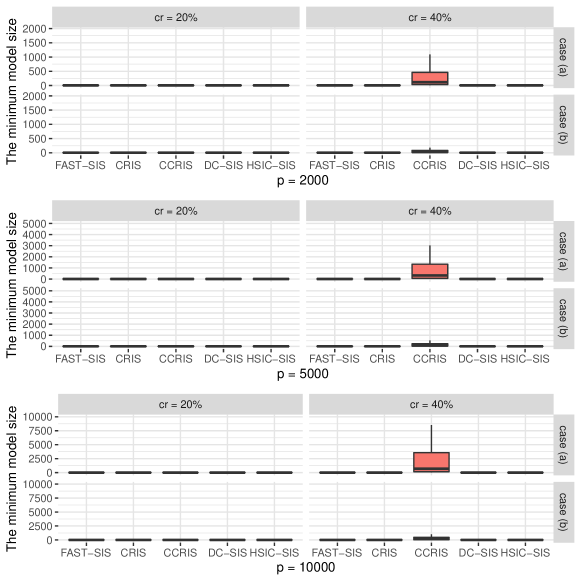
Figure 1: Boxplot of the minimum model size that are required to include all active predictors for Example 1 with the censoring rate of 20% and 40%. Case (a): random censoring, $C\sim\rm{Unif}(0,c)$; Case (b): nonrandom censoring, $C\sim\rm{Unif}(0,c\cdot\lvert Z_{1}-Z_{2}\rvert)$

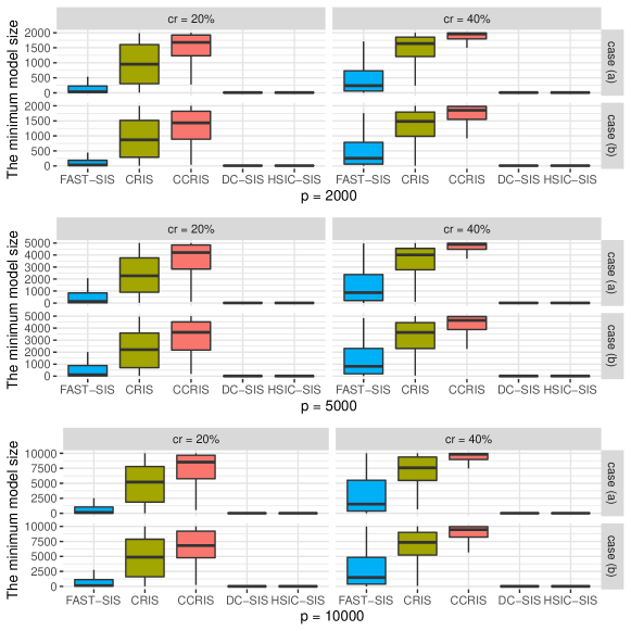
Figure 2: Boxplot of the minimum model size that are required to include all active predictors for Example 2 with the censoring rate of 20% and 40%. Case (a): random censoring, $C\sim\rm{Unif}(0,c)$; Case (b): nonrandom censoring, $C\sim\rm{Unif}(0,c\cdot\lvert Z_{1}-Z_{2}\rvert)$

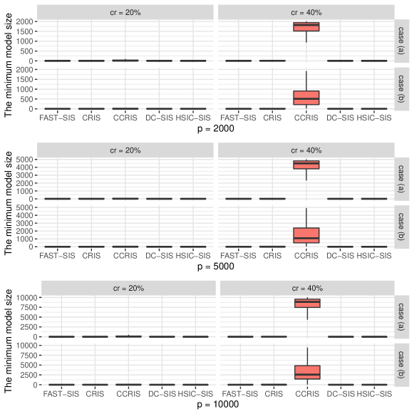
Figure 3: Boxplot of the minimum model size that are required to include all active predictors for Example 3 with the censoring rate of 20% and 40%. Case (a): random censoring, $C\sim\rm{Unif}(0,c)$; Case (b): nonrandom censoring, $C\sim\rm{Unif}(0,c\cdot\lvert Z_{1}-Z_{2}\rvert)$

To provide comprehensive insight of these methods, we further plot the boxplot of $\cal S$ out of 200 replications for Examples 1-3 in Figures 1-3. We can see clearly that the performance of the proposed HSIC-SIS procudure is robust for different settings and exhibits more satisfactory results than the other considered methods. Therefore, it could be expected to have a good application prospect in ultrahigh-dimensional survival data analysis.

4 Real Data Analysis

As an illustration, we apply the proposed screening procedure HSIC-SIS to the diffuse large-B-cell lymphoma (DLBCL) data and the ovarian cancer data. We first demonstrate the reliability and superiority of the proposed HSIC-SIS method by comparing different screening results of the well-known DLBCL data, then apply the HSIC-SIS method to the new ovarian cancer data in an attempt to identify the important RNA which affects the survival risk of ovarian cancer patients.

4.1 The analysis of DLBCL data

The diffuse large-B-cell lymphoma (DLBCL) data is a classic data which has been analyzed in the literature related to feature screening for ultrahigh-dimensional survival data. This dataset was originally collected by Rosenwald et al. (2002), including $n=240$ patients whose survival time $T$ ranged from $0$ to $21.8$ years, with a median of $2.8$ years across all samples. Of the $240$ patients, $102$ were still alive at the final follow-up visit, which led to the censoring rate of $42.5\%$. For each patient, there are $p=7399$ gene expression levels, and the goal is to find the important genes which have great influence on $T$ from $7399$ genes.

For comparison, we also consider FAST-SIS of Gorst-Rasmussen and Scheike (2013), CRIS of Song et al. (2014), CCRIS of Zhang et al. (2018), and DC-SIS of Zhang et al. (2021) to analyze this data. Specifically, we apply these five screening methods to screening the important ones among the 7399 genes and select the top $43=[240/\log(240)]$ covariates. The selection result of HSIC-SIS is largely coincides with FAST-SIS and DC-SIS, which contains 25 and 37 overlapping genes, respectively. Among the top 43 genes selected by the proposed HSIC-SIS procedure, there are 41 genes that are also considered important by at least one other screening method. Furthermore, we fit a Cox proportional hazards model based on the top 43 genes selected by HSIC-SIS, and utilize the regularization methods LASSO, SCAD and MCP to select the significant ones among these 43 covariates, where the tuning parameter is selected by the 10-fold cross-validation. The unique identifications (UNIQIDs) and the estimated value of the coefficient of selected covariates are summarized in Table 7, from which we draw similar conclusion as Zhang et al. (2021). In particular, genes 31981, 31669, 32238, 24376 and 25054 are all selected by LASSO, SCAD and MCP methods, indicating that these genes could be strongly associated with patients’ survival risk. Moreover, the gene 31981 has the greatest impact on the survival risk. In contrast, HSIC-SIS method attaches more importance to genes 27731, 28377, 27774, 29912, 24367 and 31806 rather than genes 32679, 28641 and 17902.

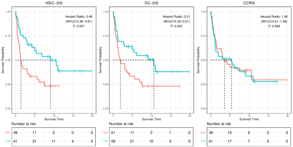
Figure 4: The Kaplan-Meier estimate of survival curves for the low-risk and high-risk groups from the testing dataset

In addition, to evaluate the predictive performance of HSIC-SIS, 240 patients are randomly divided into a training set with $n_{1}=160$ subjects and a test set with $n_{2}=80$ subjects (Rosenwald et al., 2002), where the training set is used to build the prediction model and the test data is used to evaluate the model. A summary of the survival times in the DLBCL dataset is shown in Table 8. We first apply these five screening methods to the training set and select the top $[160/\log(160)]=31$ covariates, then fit the Cox proportional hazards model on these selected covariates and perform the regularization method LASSO to further remove some irrelevant covariates, where the tuning parameters are determined by the 10-fold cross-validation. Based on the estimated value of the coefficient of selected predictors obtained from the training set, we calculate the risk scores for the patients in the testing set and divide them into low-risk and high-risk groups, where the threshold is the median of the estimated scores from the training set. Figure 4 depicts the Kaplan–Meier survival curves for each group. For brevity, we only show the Kaplan–Meier curves for the proposed procedure HSIC-SIS, and the other two methods DC-SIS, CCRIS which has the best and the worst separation among the other four screening methods. We observe that the two curves are well-separated for the proposed HSIC-SIS procedure. Objectively, we evaluate the difference between the two survival curves by the $\log$-rank test and summarize the $p$-values in Figure 4, which shows that HSIC-SIS procedure has the smallest $p$-values, indicating that HSIC-SIS procedure behaves a favorable and reliable prediction based on the final selected model.

4.2 The analysis of ovarian cancer data

Ovarian cancer is one of the three major gynecological tumors. At present, the main treatment method is ovarian cytoreductive surgery plus chemotherapy. However, secondary drug resistance often occurs. Studies have shown that genetic factors are closely related to the progression of ovarian cancer disease, while RNA plays a key role in the cell cycle. Therefore, identifying these RNAs with inducing or inhibitory effects can help target therapy to patients and improve the development strategy of new drugs. Different researchers have measured RNA expression level data of ovarian cancer patients in different years, which are summarized in the R package “OvarianCancer". We explore the GSE51088_eset dataset, which was determined by Karlan et al. (2014) by using RNA expression microarray technology. After deleting the missing values and covariates with variance 0, we obtain the survival time $T$ and $p=6844$ RNA expression levels of $n=152$ patients. The observed survival time of patients range from 30 to 7001 days, with a median of 1491 days. Among the 152 patients, 40 were still alive at the last follow-up, which led to the censoring rate of $26.32\%$.

Similarly, we apply FAST-SIS, CRIS, CCRIS, DC-SIS and HSIC-SIS to screening the important ones among the 6844 RNAs, and reserve the first $30=[152/\log(152)]$ RNAs. Among the 30 covariates selected by HSIC-SIS procedure, there are 22 RNAs overlapped with DC-SIS and 20 RNAs overlapped with CCRIS, furthermore, 23 RNAs are also considered as vital covariates by at least one other screening method.

Innovatively, we integrate the results of the five screening procedures using the voting method. Voting is an ensemble learning procedure that follows the principle of the minority obeying the majority. By integrating multiple models, voting improves the model’s robustness and generalization ability. Specifically, we build a Cox proportional hazards model using the 25 RNAs with the highest frequency in the five screening results, and utilize regularization methods LASSO, SCAD and MCP to perform further variable selection with the tuning parameters selected by the 10-fold cross-validation. The selection results for significant RNAs and the estimated value of the coefficient of selected predictors are given in Table 9, from which we can see that RNA FPR1, ATP2C2, NUDT7, SMIM14 and FAM189A2 are all selected by LASSO, SCAD and MCP, means that these five RNAs could be strongly associated with patients’ survival risk and the RNA FPR1 may have the greatest impact on the survival risk. Furthermore, we consult the literature related to the selected RNA (Ahmet et al., 2020; Yan et al., 2020; Minopoli et al., 2019; Kohn et al., 2014; Yang et al., 2020; Gendoo et al., 2019), which shows that our selection results are consistent with theirs. For example, Ahmet et al. (2020), Yan et al. (2020), Minopoli et al. (2019) emphasized the importance of RNA FPR1, where Minopoli et al. (2019) identified FPR1 as a novel and valuable marker for predicting the propensity of ovarian cancer cells to adhere and subsequently invade mesothelium, and suggested FPR1 as a new therapeutic target for the treatment of metastatic ovarian cancer. Kohn et al. (2014) found that Ca(2+)-related gene ATP2C2 exhibited highly selective expression in epithelial tumor cells. Yang et al. (2020) listed SMIM14 as a down-regulated expressed gene in ovarian cancer tissues compared to normal controls from four microarray profile datasets. Gendoo et al. (2019) found that FAM189A2 had significant role in ovarian cancer and was also identified as the only gene that is indicative of worse outcomes.

5 Conclusion

In this paper, we proposed a new model-free screening method HSIC-SIS for ultrahigh dimensional right-censored survival data based on the Hilbert-Schmidt independence criterion (HSIC). It is a model-free procedure and does not rely on any model structure, thus it works well for various types of survival models. Unlike most existing model-free screening methods for right-censored survival data, this procedure does not involve the Kaplan–Meier estimator, thus its performance is much more robust to the existence of heavy censoring or outliers. Similar to distance correlation, HSIC is also a measure of independence rather than correlation, HSIC is zero means that the random variables are independent, so its performance is better than most existing screening methods, which can also be seen from the simulation results. Moreover, the empirical estimate of HSIC is very simple as it is just the trace of a product of Gram matrices, thus the corresponding calculation of the proposed procedure is very simple and fast. The numerical results indicated that the proposed methodology works well for practical situations and has its distinctive advantages for the complicated nonlinear models which could be more feasible to capture the characteristic of the ultrahigh-dimensional survival data.

Note that the calculation of marginal utility $\widehat{\omega}_{k}$ depends on the selection of kernel function, since the goal of feature screening is to filter out a majority of inactive variables, not focus on the accuracy of parameter estimation, different kernel functions have very little influence on the screening results. In simulation studies, we considered the Gaussian kernel with $f(x,y)=\exp(-\frac{\|x-y\|^{2}}{2\gamma^{2}})$ and set $\gamma=2$. We also tried other kernel functions, such as linear kernel function and Laplacian kernel function, the proposed method also performed well, we omitted the results here to save space. Moreover, as the definition of HSIC is very complex, how to construct the sure screening property and the ranking consistency of the proposed procedure is a complex question, we leave it for further research.

There are some issues that deserve further consideration. First, similar to most marginal screening methods, the proposed method may fail to detect the hidden active variables which are jointly important but are weakly correlated with the response, how to propose a screening method using the joint information of covariates is an important issue. Moreover, if we have prior information on active covariates, how to include such information to propose more efficient screening methods merits further investigation. Finally, we considered the right-censored survival data in this paper, while in medical follow-up studies we often collect interval-censored survival data, how to extend this procedure to handle interval-censored data is also an interesting problem.

Conflict of interest

The authors declare that we have no conflict of interest.

Table 1: The simulation results for Example 1 with the censoring rate CR$=20\%$

					${\cal P}_{e}$
$p$	Case	Method	Med.	IQR	$X_{1}$	$X_{2}$	$X_{3}$	$X_{4}$	$X_{5}$	${\cal P}_{a}$
2000	(a)	FAST-SIS	5	0	1.000	1.000	1.000	1.000	1.000	1.000
		CRIS	5	0	0.995	1.000	0.995	1.000	0.985	0.980
		CCRIS	5	0	1.000	1.000	1.000	1.000	1.000	1.000
		DC-SIS	5	0	1.000	1.000	1.000	1.000	1.000	1.000
		HSIC-SIS	5	0	1.000	1.000	1.000	1.000	1.000	1.000
	(b)	FAST-SIS	5	0	1.000	1.000	1.000	1.000	1.000	1.000
		CRIS	5	0	0.985	0.995	1.000	1.000	0.980	0.965
		CCRIS	5	0	1.000	1.000	1.000	1.000	1.000	1.000
		DC-SIS	5	0	1.000	1.000	1.000	1.000	1.000	1.000
		HSIC-SIS	5	0	1.000	1.000	1.000	1.000	1.000	1.000
5000	(a)	FAST-SIS	5	0	1.000	1.000	1.000	1.000	1.000	1.000
		CRIS	5	0	1.000	1.000	1.000	1.000	0.985	0.985
		CCRIS	5	0	1.000	1.000	1.000	1.000	1.000	1.000
		DC-SIS	5	0	1.000	1.000	1.000	1.000	1.000	1.000
		HSIC-SIS	5	0	1.000	1.000	1.000	1.0000	1.000	1.000
	(b)	FAST-SIS	5	0	1.000	1.000	1.000	1.000	1.000	1.000
		CRIS	5	1	1.000	1.000	1.000	1.000	0.995	0.995
		CCRIS	5	0	1.000	1.000	1.000	1.000	1.000	1.000
		DC-SIS	5	0	1.000	1.000	1.000	1.000	1.000	1.000
		HSIC-SIS	5	0	1.000	1.000	1.000	1.000	1.000	1.000
10000	(a)	FAST-SIS	5	0	1.000	1.000	1.000	1.000	1.000	1.000
		CRIS	5	0	0.995	1.000	1.000	1.000	0.990	0.985
		CCRIS	5	0	1.000	1.000	1.000	1.000	0.995	0.995
		DC-SIS	5	0	1.000	1.000	1.000	1.000	1.000	1.000
		HSIC-SIS	5	0	1.000	1.000	1.000	1.000	1.000	1.000
	(b)	FAST-SIS	5	0	1.000	1.000	1.000	1.000	1.000	1.000
		CRIS	5	0	0.995	1.000	1.000	1.000	0.990	0.985
		CCRIS	5	1	0.995	1.000	1.000	1.000	1.000	0.995
		DC-SIS	5	0	1.000	1.000	1.000	1.000	1.000	1.000
		HSIC-SIS	5	0	1.000	1.000	1.000	1.000	1.000	1.000

Table 2: The simulation results for Example 1 with the censoring rate CR$=40\%$

					${\cal P}_{e}$
$p$	Case	Method	Med.	IQR	$X_{1}$	$X_{2}$	$X_{3}$	$X_{4}$	$X_{5}$	${\cal P}_{a}$
2000	(a)	FAST-SIS	5	0	1.000	1.000	1.000	1.000	1.000	1.000
		CRIS	5	1	0.990	1.000	0.995	0.995	0.985	0.980
		CCRIS	116	427	0.405	0.625	0.660	0.585	0.445	0.260
		DC-SIS	5	0	1.000	1.000	1.000	1.000	1.000	1.000
		HSIC-SIS	5	0	1.000	1.000	1.000	1.000	1.000	1.000
	(b)	FAST-SIS	5	0	1.000	1.000	1.000	1.000	1.000	1.000
		CRIS	5	1	0.960	0.980	0.990	0.990	0.975	0.945
		CCRIS	30	73	0.670	0.945	0.965	0.925	0.785	0.545
		DC-SIS	5	0	1.000	1.000	1.000	1.000	1.000	1.000
		HSIC-SIS	5	0	1.000	1.000	1.000	1.000	1.000	1.000
5000	(a)	FAST-SIS	5	0	1.000	1.000	1.000	1.000	1.000	1.000
		CRIS	5	1	0.990	1.000	1.000	1.000	0.970	0.965
		CCRIS	324	1278	0.335	0.470	0.525	0.510	0.330	0.190
		DC-SIS	5	0	1.000	1.000	1.000	1.000	1.000	1.000
		HSIC-SIS	5	0	1.000	1.000	1.000	1.000	1.000	1.000
	(b)	FAST-SIS	5	0	1.000	1.000	1.000	1.000	1.000	1.000
		CRIS	5	2	0.985	0.995	1.000	1.000	0.995	0.975
		CCRIS	77	206	0.455	0.825	0.890	0.835	0.615	0.325
		DC-SIS	5	0	1.000	1.000	1.000	1.000	0.998	0.998
		HSIC-SIS	5	0	1.000	1.000	1.000	1.000	1.000	1.000
10000	(a)	FAST-SIS	5	0	1.000	1.000	1.000	1.000	1.000	1.000
		CRIS	5	1	0.980	0.990	0.995	0.995	0.990	0.980
		CCRIS	698	3415	0.265	0.410	0.445	0.410	0.275	0.110
		DC-SIS	5	0	1.000	1.000	1.000	1.000	1.000	1.000
		HSIC-SIS	5	0	1.000	1.000	1.000	1.000	1.000	1.000
	(b)	FAST-SIS	5	0	1.000	1.000	1.000	1.000	1.000	1.000
		CRIS	5	2	0.955	0.995	1.000	0.995	0.965	0.920
		CCRIS	172	425	0.330	0.745	0.845	0.780	0.560	0.230
		DC-SIS	5	0	1.000	1.000	1.000	1.000	1.000	1.000
		HSIC-SIS	5	0	1.000	1.000	1.000	1.000	1.000	1.000

Table 3: The simulation results for Example 2 with the censoring rate CR$=20\%$

					${\cal P}_{e}$
$p$	Case	Method	Med.	IQR	$X_{1}$	$X_{5}$	$X_{10}$	${\cal P}_{a}$
2000	(a)	FAST-SIS	36	215	1.000	1.000	0.515	0.515
		CRIS	953	1301	0.965	0.995	0.055	0.055
		CCRIS	1678	691	0.935	0.640	0.000	0.000
		DC-SIS	9	2	1.000	1.000	0.990	0.990
		HSIC-SIS	9	2	1.000	1.000	1.000	1.000
	(b)	FAST-SIS	33	174	1.000	1.000	0.520	0.520
		CRIS	870	1225	0.970	0.995	0.050	0.050
		CCRIS	1435	930	0.820	0.575	0.010	0.000
		DC-SIS	9	2	1.000	1.000	0.995	0.995
		HSIC-SIS	9	2	1.000	1.000	1.000	1.000
5000	(a)	FAST-SIS	128	826	1.000	1.000	0.335	0.335
		CRIS	2268	2858	0.920	0.950	0.040	0.040
		CCRIS	4204	2009	0.860	0.475	0.005	0.000
		DC-SIS	10	3	0.995	1.000	0.920	0.915
		HSIC-SIS	10	3	0.985	1.000	0.935	0.920
	(b)	FAST-SIS	113	873	1.000	1.000	0.340	0.340
		CRIS	2212	2891	0.935	0.960	0.025	0.025
		CCRIS	3652	2348	0.740	0.485	0.000	0.000
		DC-SIS	10	4	0.995	1.000	0.915	0.910
		HSIC-SIS	10	3	0.985	1.000	0.925	0.915
10000	(a)	FAST-SIS	140	1028	1.000	1.000	0.320	0.320
		CRIS	5210	5930	0.945	0.985	0.010	0.010
		CCRIS	8528	3920	0.780	0.355	0.000	0.000
		DC-SIS	10	2	0.995	1.000	0.970	0.965
		HSIC-SIS	10	2	0.995	1.000	0.970	0.965
	(b)	FAST-SIS	134	1115	1.000	1.000	0.320	0.320
		CRIS	4877	6248	0.940	0.985	0.015	0.015
		CCRIS	6811	4434	0.720	0.375	0.000	0.000
		DC-SIS	10	3	0.995	1.000	0.975	0.970
		HSIC-SIS	10	3	0.995	1.000	0.980	0.975

Table 4: The simulation results for Example 2 with the censoring rate CR$=40\%$

					${\cal P}_{e}$
$p$	Case	Method	Med.	IQR	$X_{1}$	$X_{5}$	$X_{10}$	${\cal P}_{a}$
2000	(a)	FAST-SIS	239	675	1.000	1.000	0.175	0.175
		CRIS	1639	646	0.580	0.640	0.005	0.005
		CCRIS	1961	199	0.200	0.000	0.000	0.000
		DC-SIS	9	2	1.000	1.000	1.000	1.000
		HSIC-SIS	9	2	1.000	1.000	1.000	1.000
	(b)	FAST-SIS	256	725	1.000	1.000	0.170	0.170
		CRIS	1483	806	0.680	0.745	0.015	0.015
		CCRIS	1853	428	0.165	0.000	0.000	0.000
		DC-SIS	9	2	1.000	1.000	1.000	1.000
		HSIC-SIS	9	2	1.000	1.000	1.000	1.000
5000	(a)	FAST-SIS	870	2165	1.000	1.000	0.125	0.125
		CRIS	4008	1778	0.545	0.610	0.000	0.000
		CCRIS	4884	514	0.095	0.000	0.000	0.000
		DC-SIS	9	2	1.000	1.000	0.960	0.960
		HSIC-SIS	10	4	1.000	1.000	0.935	0.935
	(b)	FAST-SIS	816	2113	1.000	1.000	0.110	0.110
		CRIS	3638	2153	0.645	0.745	0.000	0.000
		CCRIS	4644	1082	0.110	0.000	0.000	0.000
		DC-SIS	9	3	1.000	1.000	0.970	0.970
		HSIC-SIS	10	4	1.000	1.000	0.945	0.945
10000	(a)	FAST-SIS	1527	5134	1.000	1.000	0.075	0.075
		CRIS	7579	3897	0.440	0.510	0.000	0.000
		CCRIS	9830	1006	0.045	0.000	0.000	0.000
		DC-SIS	9	4	1.000	1.000	0.950	0.950
		HSIC-SIS	10	7	1.000	1.000	0.905	0.905
	(b)	FAST-SIS	1486	4458	1.000	1.000	0.060	0.060
		CRIS	7348	3790	0.570	0.625	0.000	0.000
		CCRIS	9466	1744	0.070	0.000	0.000	0.000
		DC-SIS	9	4	1.000	1.000	0.960	0.900
		HSIC-SIS	10	6	1.000	1.000	0.920	0.920

Table 5: The simulation results for Example 3 with the censoring rate CR$=20\%$

					${\cal P}_{e}$
$p$	Case	Method	Med.	IQR	$X_{1}$	$X_{2}$	$X_{9}$	$X_{10}$	${\cal P}_{a}$
2000	(a)	FAST-SIS	4	0	1.000	1.000	1.000	1.000	1.000
		CRIS	4	1	0.985	0.965	0.965	1.000	0.930
		CCRIS	10	37	0.965	0.945	0.810	0.895	0.725
		DC-SIS	4	0	1.000	1.000	1.000	1.000	1.000
		HSIC-SIS	4	0	1.000	1.000	1.000	1.000	1.000
	(b)	FAST-SIS	4	0	1.000	1.000	1.000	1.000	1.000
		CRIS	4	3	0.980	0.955	0.980	1.000	0.935
		CCRIS	6	10	0.985	0.955	0.940	0.985	0.885
		DC-SIS	4	0	1.000	1.000	1.000	1.000	1.000
		HSIC-SIS	4	0	1.000	1.000	1.000	1.000	1.000
5000	(a)	FAST-SIS	4	0	1.000	1.000	1.000	1.000	1.000
		CRIS	4	6	0.965	0.950	0.950	0.995	0.880
		CCRIS	14	61	0.950	0.945	0.815	0.870	0.690
		DC-SIS	4	0	1.000	1.000	1.000	1.000	1.000
		HSIC-SIS	4	0	1.000	1.000	1.000	1.000	1.000
	(b)	FAST-SIS	4	0	1.000	1.000	1.000	1.000	1.000
		CRIS	5	7	0.960	0.935	0.925	0.995	0.850
		CCRIS	5	7	0.960	0.935	0.925	0.995	0.850
		DC-SIS	4	0	1.000	1.000	1.000	1.000	1.000
		HSIC-SIS	4	0	1.000	1.000	1.000	1.000	1.000
10000	(a)	FAST-SIS	4	0	1.000	1.000	1.000	1.000	1.000
		CRIS	5	8	0.940	0.930	0.955	0.965	0.835
		CCRIS	42	188	0.885	0.885	0.695	0.790	0.490
		DC-SIS	4	0	1.000	1.000	1.000	1.000	1.000
		HSIC-SIS	4	0	1.000	1.000	1.000	1.000	1.000
	(b)	FAST-SIS	4	0	1.000	1.000	1.000	1.000	1.000
		CRIS	5	10	0.920	0.925	0.950	0.975	0.830
		CCRIS	10	37	0.930	0.885	0.900	0.975	0.720
		DC-SIS	4	0	1.000	1.000	1.000	1.000	1.000
		HSIC-SIS	4	0	1.000	1.000	1.000	1.000	1.000

Table 6: The simulation results for Example 3 with the censoring rate CR$=40\%$

					${\cal P}_{e}$
$p$	Case	Method	Med.	IQR	$X_{1}$	$X_{2}$	$X_{9}$	$X_{10}$	${\cal P}_{a}$
2000	(a)	FAST-SIS	4	0	1.000	1.000	1.000	1.000	1.000
		CRIS	5	7	0.950	0.910	0.975	0.995	0.855
		CCRIS	1820	423	0.125	0.110	0.005	0.005	0.000
		DC-SIS	4	0	1.000	1.000	1.000	1.000	1.000
		HSIC-SIS	4	0	1.000	1.000	1.000	1.000	1.000
	(b)	FAST-SIS	4	0	1.000	1.000	1.000	1.000	1.000
		CRIS	5	12	0.925	0.930	0.940	0.985	0.840
		CCRIS	511	693	0.400	0.350	0.360	0.385	0.020
		DC-SIS	4	0	1.000	1.000	1.000	1.000	1.000
		HSIC-SIS	4	0	1.000	1.000	1.000	1.000	1.000
5000	(a)	FAST-SIS	4	0	1.000	1.000	1.000	1.000	1.000
		CRIS	5	24	0.880	0.860	0.935	1.000	0.770
		CCRIS	4500	1000	0.045	0.085	0.010	0.000	0.000
		DC-SIS	4	0	1.000	1.000	1.000	1.000	1.000
		HSIC-SIS	4	0	1.000	1.000	1.000	1.000	1.000
	(b)	FAST-SIS	4	0	1.000	1.000	1.000	1.000	1.000
		CRIS	8	33	0.900	0.900	0.910	0.985	0.755
		CCRIS	1087	1889	0.260	0.195	0.275	0.280	0.000
		DC-SIS	4	0	1.000	1.000	1.000	1.000	1.000
		HSIC-SIS	4	0	1.000	1.000	1.000	1.000	1.000
10000	(a)	FAST-SIS	4	0	1.000	1.000	1.000	1.000	1.000
		CRIS	7	44	0.835	0.835	0.955	0.980	0.725
		CCRIS	8872	2109	0.035	0.020	0.000	0.000	0.000
		DC-SIS	4	0	1.000	1.000	1.000	1.000	1.000
		HSIC-SIS	4	0	1.000	1.000	1.000	1.000	1.000
	(b)	FAST-SIS	4	0	1.000	1.000	1.000	1.000	1.000
		CRIS	11	53	0.875	0.870	0.890	0.965	0.705
		CCRIS	2572	3376	0.175	0.175	0.150	0.205	0.000
		DC-SIS	4	0	1.000	1.000	1.000	1.000	1.000
		HSIC-SIS	4	0	1.000	1.000	0.995	1.000	0.995

Table 7: The results of selected important genes for the diffuse large-B-cell lymphoma data using the regularization methods based on the HSIC-SIS procedure

LASSO			SCAD			MCP
UNIQID	EST.		UNIQID	EST.		UNIQID	EST.
31981	0.280		31981	0.400		31981	0.401
27731	-0.238		27731	-0.348		32238	0.351
32238	0.227		32238	0.344		27731	-0.341
24376	-0.150		24376	-0.220		24376	-0.233
28377	-0.150		28377	-0.218		28377	-0.228
25054	0.146		25054	0.203		25054	0.218
31669	0.134		31669	0.160		27774	-0.184
27774	-0.108		27774	-0.154		31669	0.183
31242	0.073		29912	-0.053		29912	-0.059
17154	-0.066		24367	0.043		24367	0.032
31806	0.055		31806	0.029		31806	0.013
29912	-0.052		31242	0.020
25116	0.033		25116	0.019
24203	0.033		17154	-0.010
24367	0.032		17646	0.004
23970	0.031
27267	-0.026
27592	-0.024
28532	-0.018
17646	0.017
30669	0.011
33014	0.007

Table 8: Summary of survival times in the diffuse large-B-cell lymphoma (DLBCL) dataset

Dataset	Num	Min	Max	Median	Cen($\%$)
Train	160	0	21.8	2.5	$45$
Test	80	0	19.8	3.45	$37.5$
All	240	0	21.8	2.8	$42.5$

Table 9: The results of selected important RNAs for the ovarian data using the regularization methods based on voting

LASSO			SCAD			MCP
UNIQID	EST.		UNIQID	EST.		UNIQID	EST.
FPR1	0.158		FPR1	0.143		FPR1	0.257
NUDT7	-0.140		NUDT7	-0.123		ATP2C2	-0.224
SMIM14	-0.127		FAM189A2	-0.117		NUDT7	-0.187
FAM189A2	-0.125		ATP2C2	-0.114		SMIM14	-0.075
ATP2C2	-0.119		SMIM14	-0.105		FAM189A2	-0.070
AK7	-0.079		AK7	-0.065
ACSM1	-0.057		ACSM1	-0.035
LRRC25	0.046		LRRC25	0.032
PTGIR	0.027		PTGIR	0.018
RIBC1	-0.002

References

- Ahmet et al. (2020) Ahmet, D.S., Basheer, H.A., Salem, A., Lu, D. and Afarinkia, K. (2020). Application of small molecule FPR1 antagonists in the treatment of cancers. Sci. Rep. 10, 17249.
- Cui et al. (2015) Cui, H., Li, R. and Zhong, W. (2015). Model-free feature screening for ultrahigh dimensional discriminant analysis. J. Am. Stat. Assoc. 110, 630–641.
- Fan et al. (2011) Fan, J., Feng, Y. and Song, R. (2011). Nonparametric independence screening in sparse ultra-high-dimensional additive models. J. Am. Stat. Assoc. 106, 544–557.
- Fan and Li (2011) Fan, J. and Li, R. (2001). Variable selection via nonconcave penalized likelihood and its oracle properties. J. Am. Stat. Assoc. 96, 1348–1360.
- Fan and Lv (2008) Fan, J. and Lv, J. (2008). Sure independence screening for ultrahigh dimensional feature space. J. R. Stat. Soc. Ser. B (Methodological) 70, 849–911.
- Fan et al. (2014) Fan, J., Ma, Y. and Dai, W. (2014). Nonparametric independence screening in sparse ultra-high-dimensional varying coefficient models. J. Am. Stat. Assoc. 109, 1270–1284.
- Fan et al. (2009) Fan, J., Samworth, R. and Wu, Y. (2009). Ultrahigh dimensional feature selection: Beyond the linear model. J. Mach. Learn. Res. 10, 2013–2038.
- Fan and Song (2010) Fan, J. and Song, R. (2010). Sure independence screening in generalized linear models with NP-dimensionality. Ann. Stat. 38, 3567–3604.
- Gendoo et al. (2019) Gendoo, D., Zon, M., Sandhu, V., Manem, V. S., Ratanasirigulchai, N., et al. (2019) MetaGxData: clinically annotated breast, ovarian and pancreatic cancer datasets and their use in generating a multi-cancer gene signature. Sci. Rep. 9, 8770.
- Gorst-Rasmussen and Scheike (2013) Gorst-Rasmussen, A. and Scheike, T. (2013). Independent screening for single-index hazard rate models with ultrahigh dimensional features. J. R. Stat. Soc. Ser. B (Methodological) 75, 217–245.
- Gretton et al. (2005) Gretton, A., Bousquet, O., Smola, A. and Bernhard Schölkopf. (2005). Measuring statistical dependence with Hilbert-Schmidt norms. Algorithmic Learning Theory, International Conference, Alt, Singapore, October. Springer, Berlin, Heidelberg.
- Karlan et al. (2014) Karlan B.Y., Dering J., Walsh C., et al.(2014) POSTN/TGFBI-associated stromal signature predicts poor prognosis in serous epithelial ovarian cancer. Gynecol. Oncol. 132, 334–342.
- Kohn et al. (2014) Kohn, K.W., Zeeberg, B.M., Reinhold, W.C. and Pommier, Y. (2014) Gene expression correlations in human cancer cell lines define molecular interaction networks for epithelial phenotype. Plos One 9, e99269.
- Li et al. (2012) Li, R., Zhong, W. and Zhu, L. (2012). Feature screening via distance correlation learning. J. Am. Stat. Assoc. 107, 1129–1139.
- Liu et al. (2014) Liu, J., Li, R., Wu, R. (2014). Feature selection for varying coefficient models with ultrahigh-dimensional covariates. J. Am. Stat. Assoc. 109, 266–274.
- Liu et al. (2018) Liu, Y., Zhang, J. and Zhao, X. (2018). A new nonparametric screening method for ultrahigh-dimensional survival data. Comput. Stat. Data Anal. 119, 74–85.
- Mai and Zou (2015) Mai, Q. and Zou, H. (2015). The fused Kolmogorov filter: A nonparametric model-free screening method. Ann. Stat. 43, 1471–1497.
- Minopoli et al. (2019) Minopoli, M., Botti, G., Gigantino, V. et al. (2019) Targeting the Formyl Peptide Receptor type 1 to prevent the adhesion of ovarian cancer cells onto mesothelium and subsequent invasion. J. Exp. Clin. Cancer Res. 38, 459.
- Pan et al. (2019) Pan, W., Wang, X., Xiao, W. and Zhu, H. (2019). A generic sure independence screening procedure. J. Am. Stat. Assoc. 114, 928–937.
- Rosenwald et al. (2002) Rosenwald, A., Wright, G., Chan, W., Connors, J., Campo, E., et al. (2002). The use of molecular profiling to predict survival after chemotherapy for diffuse large-b-cell lymphoma. N. Engl. J. Med. 346, 1937–1947.
- Song et al. (2014) Song, R., Lu, W., Ma, S. and Jeng, X. J. (2014). Censored rank independence screening for high-dimensional survival data. Biometrika 101, 799–814.
- Tibshirani (1996) Tibshirani, R. (1996). Regression shrinkage and selection via the Lasso. J. R. Stat. Soc. Ser. B (Methodological) 58, 267–288.
- Tibshirani (2009) Tibshirani, R. (2009). Univariate shrinkage in the Cox model for high dimensional data. Stat. Appl. Genet. .Mol. Biol. 8, 1–18.
- Wu and Yin (2015) Wu, Y. and Yin, G. (2015). Conditional quantile screening in ultrahigh-dimensional heterogeneous data. Biometrika 102, 65–76.
- Yan et al. (2020) Yan, S., Fang, J., Chen, Y. et al.(2020) Comprehensive analysis of prognostic gene signatures based on immune infiltration of ovarian cancer. BMC Cancer 20, 1205.
- Yang et al. (2020) Yang, D., He, Y., Wu, B., Deng, Y., Wang, N., Li, M. L. and Liu, Y. (2020) Integrated bioinformatics analysis for the screening of hub genes and therapeutic drugs in ovarian cancer. J. Ovarian Res. 13, 10.
- Zhang (2010) Zhang, C. H. (2010). Nearly unbiased variable selection under minimax concave penalty. Ann. Stat. 38, 894–942.
- Zhang et al. (2021) Zhang, J., Liu, Y. and Cui, H. (2021). Model-free feature screening via distance correlation for ultrahigh dimensional survival data. Stat. Pap. 62, 2711–2738.
- Zhang et al. (2017) Zhang, J., Liu, Y. and Wu, Y. (2017). Correlation rank screening for ultrahigh-dimensional survival data. Comput. Stat. Data Anal. 108, 121–132.
- Zhang et al. (2018) Zhang, J., Yin, G., Liu, Y. and Wu, Y. (2018). Censored cumulative residual independent screening for ultrahigh-dimensional survival data. Lifetime Data Anal. 24, 273–292.
- Zhao and Li (2012) Zhao, S. D. and Li, Y. (2012). Principled sure independence screening for Cox models with ultra-high-dimensional covariates. J. Multivar. Anal. 105, 397–411.
- Zhou and Zhu (2017) Zhou, T. and Zhu, L. (2017). Model-free feature screening for ultrahigh dimensional censored regression. Stat. Comput. 27, 947–961.
- Zhu et al. (2011) Zhu, L. P., Li, L., Li, R. and Zhu, L. X. (2011). Model-free feature screening for ultrahigh-dimensional data. J. Am. Stat. Assoc. 106, 1464–1475.