A Linear Weight Transfer Rule for Local Search

Abstract

The Divide and Distribute Fixed Weights algorithm (ddfw) is a dynamic local search SAT-solving algorithm that transfers weight from satisfied to falsified clauses in local minima. ddfw is remarkably effective on several hard combinatorial instances. Yet, despite its success, it has received little study since its debut in 2005. In this paper, we propose three modifications to the base algorithm: a linear weight transfer method that moves a dynamic amount of weight between clauses in local minima, an adjustment to how satisfied clauses are chosen in local minima to give weight, and a weighted-random method of selecting variables to flip. We implemented our modifications to ddfw on top of the solver yalsat. Our experiments show that our modifications boost the performance compared to the original ddfw algorithm on multiple benchmarks, including those from the past three years of SAT competitions. Moreover, our improved solver exclusively solves hard combinatorial instances that refute a conjecture on the lower bound of two Van der Waerden numbers set forth by Ahmed et al. (2014), and it performs well on a hard graph-coloring instance that has been open for over three decades.

1 Introduction

Satisfiability (SAT) solvers are powerful tools, able to efficiently solve problems from a broad range of applications such as verification [11], encryption [25], and planning [17, 9]. The most successful solving paradigm is conflict-driven clause learning (CDCL) [24, 19]. However, stochastic local search (SLS) outperforms CDCL on many classes of satisfiable formulas [23, 22, 27, 18, 6], and it can be used to guide CDCL search [7].

SLS algorithms solve SAT instances by incrementally changing a truth assignment until a solution is found or until timeout. At each step, the algorithm flips the truth value of a single boolean variable, often according to some heuristic. A common heuristic is flipping variables that reduce the number of falsified clauses in the formula, but this is not the only one. The algorithm reaches a local minimum when no variable can be flipped to improve its heuristic. At that point, the algorithm either adjusts its truth assignment or internal state to escape the local minimum, or it starts over. Refer to chapter 6 from the Handbook of Satisfiability [4] for a more detailed discussion of SLS algorithms.

Dynamic local search (DLS) algorithms are SLS algorithms that assign a weight to each clause. They then flip variables to reduce the amount of weight held by the falsified clauses. DLS algorithms escape local minima by adjusting clause weights until they can once again flip variables to reduce the amount of falsified weight.

Several DLS algorithms have been studied. For example, the Pure Additive Weighting Scheme algorithm (paws) [26] and the Scaling and Probabilistic Smoothing algorithm (saps) [14] both increase the weight of falsified clauses in local minima. A drawback of this method of escaping local minima is that the clause weights must periodically be re-scaled to prevent overflow.

The Divide and Distribute Fixed Weights algorithm (ddfw) [15] introduces an alternative way of escaping local minima: increase the weight of falsified clauses by taking weight from satisfied clauses. In local minima, ddfw moves a fixed, constant amount of weight to each falsified clause from a satisfied clause it shares at least one literal with. The transfer method keeps the total amount of clause weight constant, eliminating the need for a re-scaling phase. Another consequence of this transfer method is that as more local minima are encountered, difficult-to-satisfy clauses gather more weight. Thus, ddfw dynamically identifies and prioritizes satisfying hard clauses.

Recent work shows that ddfw is an effective algorithm. For example, ddfw (as implemented in ubcsat [28]) is remarkably effective on matrix multiplication and graph-coloring problems [13, 12]. Yet despite its success, ddfw has received little research attention. In this paper, we revisit the ddfw algorithm to study why it works well and to improve its performance.

Our contributions are as follows. We propose three modifications to the ddfw algorithm. We first introduce a linear weight transfer rule to allow for a more dynamic transfer of weight in local minima. We then adjust a performance-critical parameter that randomizes which satisfied clause gives up weight in local minima. Our adjustment is supported by an empirical analysis. Finally, we propose a new randomized method for selecting which variable to flip. We implement each of our modifications on top of the state-of-the-art SLS solver yalsat to create a new implementation of ddfw that supports parallelization and restarts. We then evaluate our solver against a set of challenging benchmarks collected from combinatorial problem instances and the past three years of SAT competitions. Our results show that our modifications boost the performance of ddfw: Our best-performing version of ddfw solves 118 SAT Competition instances, a vast improvement over a baseline of 83 solves from the original algorithm. Our solver also exhibits a 16% improvement over the baseline on a set of combinatorial instances. Moreover, in parallel mode, our solver solves instances that refute a conjecture on the lower bound of two van der Waerden numbers [2], and it matches performance with the winning SLS solver from the 2021 SAT competition on a graph-coloring instance that has been open for the past three decades.

2 Preliminaries

SAT solvers operate on propositional logic formulas in conjunctive normal form (CNF). A CNF formula $F{}=\bigwedge_{i}C_{i}$ is a conjunction of clauses, and each clause $C_{i}=\bigvee_{j}\ell_{j}$ is a disjunction of boolean literals. We write $v$ and $\overline{v}$ as the positive and negative literals for the boolean variable $v$, respectively.

A truth assignment $\alpha$ maps boolean variables to either true or false. A literal $v$ (resp. $\overline{v}$) is satisfied by $\alpha$ if $\alpha(v)$ is true ($\alpha(v)$ is false, respectively). A clause $C$ is satisfied by $\alpha$ if $\alpha$ satisfies at least one of its literals. A formula $F{}$ is satisfied by $\alpha$ exactly when all of its clauses are satisfied by $\alpha$. Two clauses $C$ and $D$ are neighbors if there is a literal $\ell$ with $\ell\in C$ and $\ell\in D$. Let $\mathrm{Neighbors}(C)$ be the set of neighbors of $C$ in $F{}$, excluding itself.

Many SLS algorithms assign a weight to each clause. Let $W:\mathcal{C}\rightarrow\mathbb{R}_{\geq 0}$ be the mapping that assigns weights to the clauses in $\mathcal{C}$. One can think of $W(C)$ as the cost to leave $C$ falsified. We call the total amount of weight held by the falsified clauses, the falsified weight. A variable that, when flipped, reduces the falsified weight is called a weight-reducing variable (wrv). A variable that doesn’t affect the falsified weight when flipped is a sideways variable (sv).

3 The ddfw Algorithm

Algorithm 1 shows the pseudocode for the ddfw algorithm. ddfw attempts to find a satisfying assignment for a given CNF formula $F$ over MAXTRIES trials. The weight of each clause is set to $w_{0}$ at the start of the algorithm. Each trial starts with a random assignment. By following a greedy heuristic method, ddfw selects and then flips weight-reducing variables until none are left. At this point, it either flips a sideways variable, if one exists and if a weighted coin flip succeeds, or it enters the weight transfer phase, where each falsified clause receives a fixed amount of weight from a maximum-weight satisfied neighbor. Occasionally, ddfw transfers weight from a random satisfied clause instead, allowing weight to move more fluidly between neighborhoods. The amount of weight transferred depends on whether the selected clause has more than $w_{0}$ weight.

1

Input: CNF Formula $F$, $w_{0}$, spt, cspt, c_> , c₌

Output: Satisfiability of $F$

2 $W(C)\leftarrow w_{0}$ for all $C\in F$

3 for $t=1$ to MAXTRIES do

4    $\alpha\leftarrow$ random truth assignment on the variables in $F$

5    for $f=1$ to MAXFLIPS do

6       if $\alpha$ satisfies $F$ then return “SAT”

7       else

8          if there is a wrv then

9             Flip a wrv that most reduces the falsified weight

10            

11             else if there is a sv and rand $\leq\texttt{spt}$ then

12                Flip a sideways variable

13               

14                else

15                   foreach falsified clause $C$ do

16                      $C_{s}\leftarrow$ maximum-weighted satisfied clause in $\mathrm{Neighbors}(C)$

17                      if $W(C_{s})<w_{0}$ or rand $\leq\texttt{cspt}$ then

18                         $C_{s}\leftarrow$ random satisfied clause with $W\geq w_{0}$

19                        

20                         if $W(C_{s})>w_{0}$ then

21                            Transfer c_> weight from $C_{s}$ to $C$

22                           

23                            else

24                               Transfer c₌ weight from $C_{s}$ to $C$

25                              

26                              

27                              

28                              

29                              

30                              

31                               return “No SAT”

Algorithm 1 The ddfw algorithm

There are five parameters in the original ddfw algorithm: the initial weight $w_{0}$ given to each clause, the two weighted-coin thresholds spt and cspt for sideways flips and transfers from random satisfied clauses, and the amount of weight to transfer in local minima c_> and c₌ . In the original ddfw paper, these five values are fixed constants, with $w_{0}=8$, $\texttt{spt}{}=0.15$, $\texttt{cspt}{}=0.01$, $\texttt{c}_{>}=2$, and $\texttt{c}_{=}=1$.

ddfw is unique in how it transfers weight in local minima. Similar SLS algorithms increase the weight of falsified clauses (or decrease the weight of satisfied clauses) globally; weight is added and removed based solely on whether the clause is satisfied. ddfw instead moves weight among clause neighborhoods, with falsified clauses receiving weight from satisfied neighbors.

One reason why this weight transfer method may be effective is that satisfying a falsified clause $C$ by flipping literal $\overline{\ell}$ to $\ell~{}(\in C)$ increases the number of true literals in satisfied clauses that neighbor $C$ on $\ell$. Thus, $C$ borrows weight from satisfied clauses that tend to remain satisfied when $C$ itself becomes satisfied. As a result, ddfw satisfies falsified clauses while keeping satisfied neighbors satisfied.

The existence of two weight transfer parameters c_> and c₌ deserves discussion. Let heavy clauses be those clauses $C$ with $W(C)>w_{0}$. Lines 16-19 in Algorithm 1 allow for a different amount of weight to be taken from heavy clauses than from clauses with the initial weight. Because lines 14-15 ensure that the selected clause $C_{s}$ will have at least $w_{0}$ weight, c₌ is used when $W(C_{s})=w_{0}$ and c_> is used when $W(C_{s})>w_{0}$ (hence the notation). The original algorithm sets $\texttt{c}_{>}=2$ and $\texttt{c}_{=}=1$, which has the effect of taking more weight from heavy clauses.

4 Solvers, Benchmarks, and Hardware

The authors of the original ddfw algorithm never released their source code or any binaries. The closest thing we have to a reference implementation is the one in the SLS SAT-solving framework ubcsat [27, 28]. We call this implementation ubc-ddfw, and we use it as a baseline in our experiments.

Unfortunately, ubc-ddfw cannot be extended to implement our proposed modifications due to its particular architecture. Instead, we implemented ddfw on top of yalsat [5], which is currently one of the strongest local search SAT solvers. For example, it is the only local search solver in Mallob-mono [21], the clear winner of the cloud track in the SAT Competitions of 2020, 2021, and 2022. yalsat uses probsat [3] as its underlying algorithm, which flips variables in falsified clauses drawn from an exponential probability distribution.

One benefit of implementing ddfw on top of yalsat is that is yalsat supports parallelization, which can be helpful when solving challenging formulas. In our experiments, we compare our implementation of ddfw to ubc-ddfw to verify that the two implementations behave similarly.

Our implementation of ddfw on top of yalsat was not straightforward. First, we switched the underlying SLS algorithm from probsat to ddfw. Then we added additional data structures and optimizations to make our implementation efficient. For example, one potential performance bottleneck for ddfw is calculating the set of weight-reducing variables for each flip. Every flip and adjustment of clause weight can change the set, so the set must be re-computed often. A naive implementation that loops through all literals in all falsified clauses is too slow, since any literal may appear in several falsified clauses, leading to redundant computation. Instead, we maintain a list of variables uvars that appear in any falsified clause. After each flip, this list is updated. To compute the set of weight-reducing variables, we iterate over the variables in uvars, hitting each literal once. In this way, we reduce redundant computation.

Adding our proposed modifications to our implementation was simpler. We represent clause weights with floating-point numbers, and the linear weight transfer rule replaced the original one. We also made the variable selection and weight transfer methods modular, so our modifications slot in easily.

We evaluated our implementations of ddfw against two benchmarks. The Combinatorial (COMB) set consists of 65 hard instances from the following eight benchmarks families collected by Heule: (i) $\mathtt{26x26}$ (4 grid positioning instances), (ii) $\mathtt{asias}$ (2 almost square packing problems), (iii) $\mathtt{MM}$ (20 matrix multiplication instances), (iv) $\mathtt{mphf}$ (12 cryptographic hash instances), (v) $\mathtt{ptn}$ (2 Pythagorean triple instances), (vi) Steiner (3 Steiner triples cover instances [20]), (vii) $\mathtt{wap}$ (9 graph-coloring instances [16]), and (viii) $\mathtt{vdw}$ (13 van der Waerden number instances). These benchmarks are challenging for modern SAT solvers, including SLS solvers. The $\mathtt{wap}$ benchmark contains three instances that have been open for three decades, and $\mathtt{vdw}$ contains two instances that, if solved, refute conjectures on lower-bounds for two van der Waerden numbers [2].

The SAT Competition (SATComp) set consists of all 1,174 non-duplicate main-track benchmark instances from the 2019 SAT Race and the 2020 and 2021 SAT Competitions. The competition suites contain medium-hard to very challenging benchmarks, most of which are contributed by the competitors.

Unless otherwise specified, we used a timeout of 18,000 and 5,000 seconds for the COMB and SATComp instances, respectively, in our experiments.

We used the StarExec cluster [1], where each node has an Intel CPU E5 CPU with a 2.40 GHz clock speed and a 10240 KB cache. For experiments in this cluster, we used at most 64 GB of RAM. To perform experiments on the 3 open $\mathtt{wap}$ and 2 $\mathtt{vdw}$ instances, we used a different cluster with the following specifications: two AMD EPYC 7742 CPUs with a 3.40 GHz clock speed, each with 64 cores, 256 MB of L3 cache, and 512 GB of RAM.

5 Modifications to the ddfw Algorithm

We propose three modifications to ddfw. The first is a linear rule for transferring a dynamic amount of weight in local minima. The second is an adjustment of the cspt parameter. The third is the introduction of a weighted-random method for selecting which variable to flip.

5.1 The Linear Weight Transfer Rule

The reference implementation of ddfw, ubc-ddfw, represents its clause weights as integers and transfers fixed integer weights in local minima. While this design decision allows ubc-ddfw to have a fast implementation, it unnecessarily restricts the amount of weight transferred in local minima to be integer-valued. In addition, the choice to transfer a fixed, constant amount of weight prevents ddfw from adapting to situations where more weight must be transferred to escape a local minimum, thus requiring multiple weight transfer rounds. To address these concerns, we propose a dynamic linear weight transfer rule to operate on floating-point-valued clause weights.

Let $C_{S}$ be the selected satisfied clause from which to take weight in a local minimum, as in line 13 in Algorithm 1. Our new rule transfers

$$\texttt{a}{}*W(C_{S})+\texttt{c}{}$$

weight, where $0\leq\texttt{a}{}\leq 1$ is a multiplicative parameter and $\texttt{c}{}\geq 0$ is an additive parameter.

It is not clear that the addition of a multiplicative parameter is helpful, nor what a good pair of $(\texttt{a},\texttt{c})$ values would be. So, we performed a parameter search with our solver for $\texttt{a}\in[0,0.2]$ in steps of 0.05 and $\texttt{c}\in[0,2]$ in steps of 0.25 for both of our instance sets with a 900 second timeout per run. (A parameter search using all 1,174 instances in the SATComp set was not feasible. We instead did the search on the 168 instances from SATComp set that were solved by some setting in earlier experimentation. In Section 6, all instances are used.) The PAR-2 scores for the SATComp and COMB benchmark sets for each pair of $(\texttt{a},\texttt{c})$ values are shown in Figure 1.

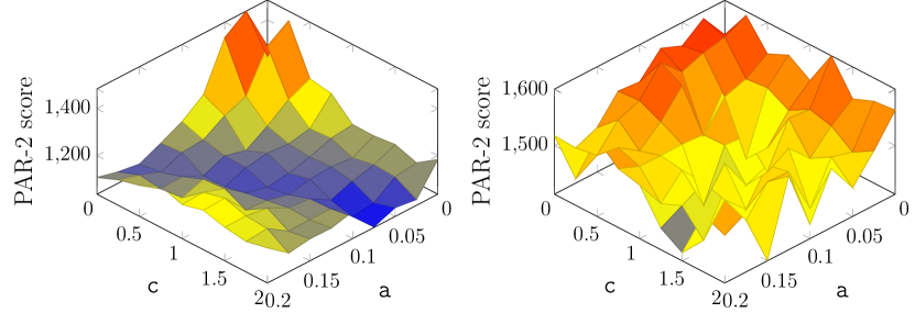
Figure 1: Parameter searches for $\texttt{a}\in[0,0.2]$ in steps of 0.05 and $\texttt{c}\in[0,2]$ in steps of 0.25 on the SATComp (left plot) and COMB (right plot) instances. A lower PAR-2 score is better. There is not a datum for $(\texttt{a},\texttt{c})=(0,0)$ since no weight would be transferred.

The plots in Figure 1 show that values of a and c close to 0 degrade performance, likely due to the need for many weight-transfer rounds to escape local minima. The beneficial effect of higher values of a and c is more pronounced in the parameter search on the SATComp instances (the left plot). Since the best-performing settings have nonzero a and c values, we infer that both parameters are needed for improved performance.

5.2 How Much Weight Should be Given Away Initially?

On lines 16-19 of Algorithm 1, ddfw takes c_> weight away from the selected clause $C_{s}$ if $C_{s}$ is heavy and c₌ weight otherwise. The linear rule introduced above can similarly be extended to four parameters: $\texttt{a}_{>}$, $\texttt{a}_{=}$, $\texttt{c}_{>}$, and $\texttt{c}_{=}$.

In the original ddfw paper, c_> (= 2) is greater than c₌ (= 1), meaning that heavy clauses give away more weight than clauses with the initial weight in local minima. The intuition behind this is simple: clauses with more weight should give away more weight. For the extended linear rule, one could adopt a similar strategy by setting a_> greater than a₌ and c_> greater than $\texttt{c}_{=}$.

However, one effect of our proposed linear rule is that once clauses give or receive weight, they almost never again have exactly $w_{0}$ weight. As a result, the parameters a₌ and c₌ control how much weight a clause gives away initially. Since the maximum-weight neighbors of falsified clauses tend to be heavy as the search proceeds, the effect of a₌ and $\texttt{c}_{=}$ diminishes over time, but they remain important at the start of the search and for determining how much weight the algorithm has available to assign to harder-to-satisfy clauses. The findings in a workshop paper [8] by two co-authors of this paper indicate that ddfw achieves a better performance when clauses initially give more weight. These findings suggest setting c₌ greater than c_> and a₌ greater than $\texttt{a}_{>}$. In Section 6, we evaluate ddfw on the extended linear rule and investigate whether clauses should initially give away more or less weight.

5.3 The cspt Parameter

On lines 14-15 of Algorithm 1, ddfw sometimes discards the maximum-weight satisfied neighboring clause $C_{s}$ and instead selects a random satisfied clause. The cspt parameter controls how often the weighted coin flip on line 14 succeeds. Though these two lines may appear to be minor, a small-scale experiment revealed that the cspt parameter is performance-critical. We ran our implementation of the original ddfw algorithm on the COMB set with an 18,000 second timeout. When we set cspt to 0, meaning that falsified clauses received weight solely from satisfied neighbors, it solved a single instance; when we set cspt to 0.01 (the value in the original ddfw algorithm), it solved 21 instances.

Among the eight families in COMB, the $\mathtt{wap}$ family was the most sensitive to the change of cspt value from 0 (solved 0) to 0.01 (solved 6 out of 9). We isolated these nine instances and ran a parameter search on them for $\texttt{cspt}{}\in[0.01,1]$ in steps of 0.01, for a total of 900 runs. We used an 18,000 second timeout per run. The PAR-2 scores are reported in Figure 2.

In Figure 2, we observe that cspt values near 0 and above 0.2 cause an increase in the PAR-2 score. These results indicate that ddfw is sensitive to the cspt value and that the cspt value should be set higher than its original value of 0.01, but not too high, which could potentially degrade the performance of the solver. We use these observations to readjust the cspt parameter in our empirical evaluation presented in Section 6.

Figure 2: The impact of cspt values on the performance of ddfw on the $\mathtt{wap}$ instances.

5.4 A Weighted-random Variable Selection Method

On line 8 of Algorithm 1, ddfw flips a weight-reducing variable that most reduces the amount of falsified weight. Such a greedy approach may prevent ddfw from exploring other, potentially better areas of the search space. Inspired by probsat, which makes greedy moves only some of the time, we introduce a new randomized method that flips a weight-reducing variable according to the following probability distribution:

$$\mathbb{P}(\text{Flipping {wrv}{} }v)=\frac{\Delta W(v)}{\sum_{v\in\texttt{wrv}}\Delta W(v)},$$

where $\Delta W(v)$ is the reduction in falsified weight if $v$ is flipped.

6 Empirical Evaluation

In this section, we present our empirical findings. Since we evaluated several different solvers, we refer to the solvers by the following names: the ubcsat version of ddfw is ubc-ddfw, the version of yalsat that implements probsat is yal-prob, and our implementation of ddfw on top of yalsat is yal-lin. In all of our experiments, we use the default random seed present in each solver, and we set the initial clause weight $w_{0}{}=8$, as in the original ddfw paper.

In our experiments with yal-lin, we varied the configuration of the solver according to our proposed modifications. We use the identifying string W-cC-P to refer to a configuration for yal-lin, where $\texttt{W}\in\{\texttt{fw}{},\texttt{lw}{}\}$ is the weight transfer method (fw stands for “fixed weight,” lw for “linear weight”), $\texttt{C}\in\{0.01,0.1\}$ is the cspt value, and $\texttt{P}\in\{\texttt{grdy}{},\texttt{wrnd}{}\}$ is the variable selection method (grdy stands for the original “greedy” method, and wrnd stands for our proposed “weighted random” method). For example, the string fw-c.01-grdy describes the original ddfw algorithm, with $\texttt{c}_{>}=2$ and $\texttt{c}_{=}=1$.

6.1 Evaluation Without Restarts

We evaluate how yal-lin performs without restarts, meaning that ddfw runs until timeout without starting from a fresh random assignment. To disable restarts, we set MAXTRIES to 1 and MAXFLIPS to an unlimited number of flips. For the COMB and SATComp benchmark sets, we set a timeout of 18,000 and 5,000 seconds, respectively.

We first checked that our solver yal-lin (with configuration fw-c.01-grdy) behaves similarly to the baseline implementation, ubc-ddfw. The solvers performed almost identically on the two benchmark sets: ubc-ddfw solved 22 of the COMB instances and 80 of the SATComp instances; yal-lin solved 21 and 83, respectively. We attribute the slight difference in solve counts to random noise. These results indicate that we implemented yal-lin correctly.

We next evaluate how yal-lin performs under changes in the cspt value and variable selection method. We run yal-lin with the fixed weight transfer method on both benchmarks with all four combinations of $\texttt{C}\in\{0.01,0.1\}$ and $\texttt{P}\in\{\texttt{grdy}{},\texttt{wrnd}{}\}$. The solve counts and PAR-2 scores are shown in Table 1.

Isolating just the change in variable selection method (scanning across rows in Table 1), we see that the weighted-random method outperforms the greedy method for each benchmark and cspt value. There is improvement both in the solve count (ranging from an additional 1 to 5 solves) and in the PAR-2 score. While the improvements may be random noise, the results indicate that injecting some randomness into how variables are flipped may lead to better performance.

Isolating the change in cspt value (scanning down columns in Table 1), we see that the higher cspt value of 0.1 outperforms the cspt value of 0.01. Improvements range from 1 additional solve to 16 additional solves. We note that the improvements when increasing the cspt value are more pronounced than when changing the variable selection method, which gives further evidence that the cspt value is performance-critical. In Section 7, we present a possible explanation for why the cspt parameter is so important.

Table 1: Solve counts and PAR-2 scores for different configurations of yal-lin. The configurations vary the cspt value and the variable selection method, with the weight transfer method being fw. The best configuration for each benchmark is bolded.

	COMB				SATComp
cspt	grdy		wrnd		grdy		wrnd
value	#solved	PAR-2	#solved	PAR-2	#solved	PAR-2	#solved	PAR-2
0.01	21	25393	24	23871	83	9339	87	9312
0.1	24	23137	25	22538	98	9223	103	9188

The linear weight transfer rule. As we noted in Section 5.2, the linear weight transfer rule can be extended to include four parameters: two multiplicative and two additive. We tested yal-lin on three particular settings of these four parameters, which we call lw-itl (linear weight initial transfer low), lw-ith (linear weight initial transfer high), and lw-ite (linear weight initial transfer equal).

• lw-itl takes a low initial transfer from clauses in local minima by setting a₌ < a_> and c₌ < c_> .

• lw-ith takes a high initial transfer from clauses in local minima by setting a₌ > a_> and c₌ > c_> .

• lw-ite does not distinguish clauses by weight, and sets the two pairs of parameters equal.

In the left plot of Figure 1, a values for the top 10% of the settings (by PAR-2 scores) are in the range [0.05, 0.1]. Hence, we use 0.05 and 0.1 as the values for a_> and a₌ in lw-itl and lw-ith. We keep the values for c_> and c₌ at 2 and 1, following the original ddfw algorithm. For lw-ite, we take the average of the two pairs of values, with $\texttt{a}_{>}=\texttt{a}_{=}=0.075$ and $\texttt{c}_{>}=\texttt{c}_{=}=1.75$. Table 2 shows the parameter values for the three configurations that we tested.

Table 2: Parameter values for three versions of linearwt

linearwt versions	a>	a=	c>	c=
lw-itl	0.1	0.05	2	1
lw-ite	0.075	0.075	1.75	1.75
lw-ith	0.05	0.1	1	2

We compare our three new configurations against the original one across the two variable selection methods. We set cspt = 0.1, as our prior experiment showed it to be better than 0.01. Table 3 summarizes the results.

Table 3: Solve counts and PAR-2 scores for different configurations of yal-lin. The configurations vary the linear weight transfer method while keeping the cspt value fixed at 0.1. The best configuration for each benchmark is bolded.

Weight Transfer Method	COMB				SATComp
	grdy		wrnd		grdy		wrnd
	#solved	PAR-2	#solved	PAR-2	#solved	PAR-2	#solved	PAR-2
fixedwt	24	23871	25	22538	98	9223	103	9188
lw-itl	26	22256	27	21769	98	9237	104	9189
lw-ite	28	21233	27	22228	111	9129	113	9114
lw-ith	26	22142	28	21338	115	9082	118	9055

Scanning down the columns of Table 3, we see that all three linear weight configurations perform at least as well as the fixed weight version, regardless of variable selection method. The improvements on the COMB benchmark are modest, with at most 4 additional solved instances. The improvements on the SATComp benchmark are more substantial, with a maximum of 17 additional solved instances.

Overall, the best-performing linear weight configuration was lw-ith, which transfers the more weight from clauses with the initial weight. These results support prior findings that more weight should be freed up to the falsified clauses in local minima. The best-performing variable selection method continues to be the weighted random method wrnd.

Figure 3: Performance profiles of yal-lin (fw-c.01-grdy) and nine modifications for COMB (left) and SATComp (right).

Analysis of solve count over runtime. In addition to solve counts and PAR-2 scores for the three linear weight configurations, we report solve counts as a function of solving time. The data for ten experimental settings of yal-lin on the two benchmarks are shown in Figure 3. Note that the original ddfw setting is represented by the setting fw-c.01-grdy, and is our baseline.

For the COMB benchmark (Figure 3, left plot), all nine other settings (our modifications) outperform the baseline in terms of solving speed and number of solved instances. The best settings are lw-ith-c.1-wrnd and lw-ite-c.1-grdy, which perform on par with each other and solve 28 instances by timeout. For the SATComp benchmark (Figure 3, right plot), the dominance of the setting lw-ith-c.1-wrnd is more pronounced. For about the first 1,000 seconds, this setting performs similar to lw-ith-c.1-grdy. After that, however, it begins to perform the best of all the settings, and it ends up solving the most instances by timeout, at 118. The baseline setting fw-c.01-grdy ends up solving 83 instances at timeout, which is 35 less than lw-ith-c.1-wrnd.

These two plots clearly show that our modifications substantially improve the original ddfw algorithm.

Figure 4: Solve time comparisons between base yal-prob, and 10 yal-lin settings for COMB and SATComp, where restarts are enabled

6.2 Evaluation With Restarts

Many SLS algorithms restart their search with a random assignment after a fixed number of flips. By default, yalsat also performs restarts. However, at each restart, yalsat dynamically sets a new restart interval as $r=100,000x$ for some integer $x\geq 1$, which is initialized to 1, and updated after each restart as follows: if $x$ is power of 2, then $x$ is set to 1, otherwise to $2*x$. The way yalsat initializes its assignment at restart also differs from many SLS algorithms. On some restarts, yalsat uses the best cached assignment. For all others, it restarts with a fresh random assignment. In this way, it attempts to balance exploitation and exploration.

We also evaluated yal-lin with yalsat-style restarts. On a restart, the adjusted clause weights are kept. The hope is that the adjusted weights help the solver descend the search landscape faster.

We compare yal-prob against ten experimental settings of yal-lin with restarts enabled. The best solver in this evaluation is yal-lin with the setting lw-ith-c.1-grdy on the COMB benchmark and the setting lw-ith-c.1-wrnd on the SATComp benchmark, which solve 11 and 49 more instances than yal-prob, respectively. Figure 4 shows solve counts against solving time, and it confirms that all the yal-lin settings solve instances substantially faster than yal-prob.

6.3 Solving Hard Instances

Closing wap-07a-40. The $\mathtt{wap}$ family from the COMB benchmark contains three open instances: wap-07a-40, wap-03a-40 and wap-4a-40. We attempted to solve these three instances using the parallel version of yal-lin with the ten yal-lin settings (without restarts) used in Section 6.1 in the cluster node with 128 cores and 18,000 seconds of timeout. All of our settings except fw-c.01-grdy (the baseline) solve the wap-07a-40 instance. The best setting for this experiment was lw-itl-c.1-wrnd, which solves wap-07a-40 in just 1168.64 seconds. However, we note that lstech_maple (LMpl) [30], the winner of the SAT track of the SAT Competition 2021, also solves wap-07a-40, in 2,103.12 seconds, almost twice the time required by our best configuration lw-itl-c.1-wrnd for solving this instance. Thus, for solving this open instance, our best setting compares well with the state-of-the-art solver for solving satisfiable instances.

With restarts, the setting lw-itl-c.1-wrnd, the best setting for this experiment, were not able to solve any of these three instances.

New lower bounds for van der Waerden/Green numbers. The van der Waerden theorem [29] is a theorem about the existence of monochromatic arithmetic progressions among a set of numbers. It states the following: there exists a smallest number $n=W(k;t_{1},\dots,t_{i},\dots,t_{k})$ such that any coloring of the integers $\{1,2,\dots,n\}$ with $k$ colors contains a progression of length $t_{i}$ of color $i$ for some $i$. In recent work, Ben Green showed that these numbers grow much faster than conjectured and that their growth can be observed in experiments [10]. We therefore call the CNF formulas to determine these numbers Green instances.

Ahmed et al. studied 20 van der Waerden numbers $W(2;3,t)$ for two colors, with the first color having arithmetic progression of length 3 and the second of length $19\leq t\leq 39$, and conjectured that their values for $t\leq 30$ were optimal, including $W(2;3,29)=868$ and $W(2,3,30)=903$ [2]. By using yal-lin, we were able to refute these two conjectures by solving the formulas Green-29-868-SAT and Green-30-903-SAT in the COMB set. Solving these instances yields two new bounds: $W(2;3,29)\geq 869$ and $W(2;3,30)\geq 904$.

To solve these two instances, we ran our various yal-lin configurations (without restarts) using yalsat’s parallel mode, along with a number of other local search algorithms from ubcsat, in the same cluster we used to solve wap-07a-40. Among these solvers, only our solver could solve the two instances. lw-itl-c.1-wrnd solved both Green-29-868-SAT and Green-30-903-SAT, in 942.60 and 6534.56 seconds, respectively. The settings lw-ith-c.1-wrnd and lw-ite-c.1-wrnd also solved Green-29-868-SAT in 1374.74 and 1260.16 seconds, respectively, but neither could solve Green-30-903-SAT within a timeout of 18,000 seconds. The CDCL solver LMpl, which solves wap-07a-40, could not solve any instances from the Green family within a timeout of 18,000 seconds.

With restarts lw-itl-c.1-wrnd, the best setting for this experiment only solves Green-29-868-SAT in 2782.81 seconds within a timeout of 18,000 seconds.

7 Discussion and Future Work

In this paper, we proposed three modifications to the DLS SAT-solving algorithm ddfw. We then implemented ddfw on top of the SLS solver yalsat to create the solver yal-lin, and we tested this solver on a pair of challenging benchmark sets. Our experimental results showed that our modifications led to substantial improvement over the baseline ddfw algorithm. The results show that future users of yal-lin should, by default, use the configuration lw-ith-c.1-wrnd.

While each modification led to improved performance, the improvements due to each modification were not equal. The performance boost due to switching to the weighted-random variable selection method was the weakest, as it resulted in the fewest additional solves. However, our results indicate that making occasional non-optimal flips may help ddfw explore its search space better.

The performance boost due to adjusting the cspt value was more substantial, supporting our initial findings in Section 5.3. One metric that could explain the importance of a higher cspt value is a clause’s degree of satisfaction (DS), which is the fraction of its literals that are satisfied by the current assignment. We noticed in experiments on the COMB benchmark with cspt = 0.01 that clauses neighboring a falsified clause had an average DS value of 0.33, while clauses without a neighboring falsified clause had an average DS value of 0.54. If this trend holds for general yal-lin runs, then it may be advantageous to take weight from the latter clauses more often, since flipping any literal in a falsified clause will not falsify any of the latter clauses. A higher cspt value accomplishes this. However, we did not investigate the relationship between DS and cspt further, and we leave this to future work. Performance also improved with the switch to a linear weight transfer method. The best method, lw-ith, supports the findings from the workshop paper that ddfw should transfer more weight from clauses with the initial weight. Future work can examine whether the heavy-clause distinction is valuable; a weight transfer rule that doesn’t explicitly check if a clause is heavy would simplify the ddfw algorithm.

When restarts are enabled, all ten settings in yal-lin perform better for COMB than when restarts are disabled. This better performance with restarts comes from solving several $\mathtt{MM}$ instances, for which these settings without restarts solve none of them. However, for SATComp, yal-lin performs better when restarts are disabled. Since SATComp comprises of substantially larger number of heterogeneous benchmarks than COMB, these results suggest that the new system performs better when restarts are disabled.

Future work on weight transfer methods can take several other directions. Different transfer functions can be tested, such as those that are a function of the falsified clause’s weight or those based on rational or exponential functions. Alternate definitions for neighboring clauses are also possible. For example, in formulas with large neighborhoods, it may be advantageous to consider clauses neighbors if they share $k>1$ literals, rather than just 1.

Figure 5: Comparison of sideways moves count per 10,000 flips with Search Progression for our baseline (fw-c.01-grdy) and best setting (lw-ith-c.1-wrnd) from yal-lin for an COMB instance sted2_0x0_n219-342

Throughout this paper, we kept the spt parameter set to 0.15. Yet, when clause weights are floating point numbers, it is rare for our solver to make sideways moves. This evident in Figure 5, which compares count of sideways moves per 10,000 flips between our baseline setting (fw-0.01-grdy), and best setting (lw-ith-c.1-wrand) for a randomly chosen SATComp instance sted2_0x0_n219-342 up to 5 millions flips. With fw-0.01-grdy, yal-lin makes some sideways moves, albeit rarely. However, with floating weight transfer in lw-ith-c.1-wrand, the solver makes almost no sideways moves as search progresses. We further investigated the effect of sideways moves on solver performance. We tested the setting lw-ith-c.1-wrnd against a version that did not perform sideways moves on the SATComp benchmark. The version with sideways moves solved 118 instances, while the version without them solved 113. This suggests that sideways moves may add a slight-but-beneficial amount of random noise to the algorithm. Future work can more fully investigate the effect of sideways moves on ddfw. One goal is to eliminate the parameter entirely in order to simplify the algorithm. Alternatively, the algorithm could be modified to occasionally flip variables that increase the falsified weight to help ddfw explore the search space.

Overall, we find that the ddfw algorithm continues to show promise and deserves more research interest. Our solver closed several hard instances that eluded other state-of-the-art solvers, and the space of potential algorithmic improvements remains rich.

Appendix 0.A Experimental Results with a Different Seed

For all our previous experiments, we used the default seed (seed of 0) used in the solvers. We have repeated the experiments reported in Section 6.1 and 6.2 for COMB and SATComp with a seed of 123. Here, we present the results with this changed seed value.

Figure 6 and 7 compare the performance of various configurations of yal-lin against their baselines for this changed seed, without restarts and with restarts, respectively. With the changed seeds, when yal-lin does not perform restarts (Figure 6), all of our configurations performs better than the baseline fw-c.01-grdy, except fw-c.01-wrnd. Similar to the results with seed 0, with the seed of 123, the configurations implementing linearwt dominates over the configurations with fixedwt. When restarts are enabled (Figure 7), with seed 123, the overall performance of our configurations are similar to what they are with seed 0 (Figure 4).

Figure 6: Performance profiles of yal-lin (fw-c.01-grdy) and nine modifications for COMB (left) and SATComp (right) with seed 123

Figure 7: Solve time comparisons between base yal-prob, and 10 yal-lin settings for COMB and SATComp with seed 123, where restarts are enabled

References

- [1] Aaron Stump, Geoff Sutcliffe, C.T.: StarExec. https://www.starexec.org/starexec/public/about.jsp (2013)
- [2] Ahmed, T., Kullmann, O., Snevily, H.S.: On the van der Waerden numbers w(2; 3, t). Discrete Applied Mathematics 174, 27–51 (2014). https://doi.org/10.1016/j.dam.2014.05.007
- [3] Balint, A.: Engineering stochastic local search for the satisfiability problem. Ph.D. thesis, University of Ulm (2014)
- [4] Biere, A., Heule, M., van Maaren, H., Walsh, T.: Handbook of Satisfiability: Volume 185 Frontiers in Artificial Intelligence and Applications. IOS Press, Amsterdam, The Netherlands (2009)
- [5] Biere, A.: YalSAT Yet Another Local Search Solver. http://fmv.jku.at/yalsat/ (2010)
- [6] Cai, S., Luo, C., Su, K.: CCAnr: A configuration checking based local search solver for non-random satisfiability. In: Heule, M., Weaver, S. (eds.) Theory and Applications of Satisfiability Testing – SAT 2015. pp. 1–8. Springer International Publishing, Cham (2015)
- [7] Cai, S., Zhang, X., Fleury, M., Biere, A.: Better Decision Heuristics in CDCL through Local Search and Target Phases. Journal of Artificial Intelligence Research 74, 1515–1563 (2022)
- [8] Codel, C.R., Heule, M.J.: A Study of Divide and Distribute Fixed Weights and its Variants. In: Pragmatics of SAT 2021 (2021)
- [9] Feng, N., Bacchus, F.: Clause size reduction with all-UIP learning. In: Pulina, L., Seidl, M. (eds.) Proceedings of SAT-2020. pp. 28–45 (2020)
- [10] Green, B.: New lower bounds for van der Waerden numbers (2021). https://doi.org/10.48550/ARXIV.2102.01543
- [11] Gupta, A., Ganai, M.K., Wang, C.: SAT-based verification methods and applications in hardware verification. In: Proceedings of SFM 2006. pp. 108–143 (2006)
- [12] Heule, M.J.H., Karahalios, A., van Hoeve, W.: From cliques to colorings and back again. In: Proceedings of CP-2022. pp. 26:1–26:10 (2022)
- [13] Heule, M.J.H., Kauers, M., Seidl, M.: New ways to multiply 3x3-matrices. J. Symb. Comput. 104, 899–916 (2019)
- [14] Hutter, F., Tompkins, D.A.D., Hoos, H.H.: Scaling and probabilistic smoothing: Efficient dynamic local search for SAT. In: Hentenryck, P.V. (ed.) Proceedings of CP 2002. pp. 233–248 (2002)
- [15] Ishtaiwi, A., Thornton, J., Sattar, A., Pham, D.N.: Neighbourhood clause weight redistribution in local search for SAT. In: Proceedings of CP-2005. pp. 772–776. Lecture Notes in Computer Science (2005)
- [16] Johnson, D.J., Trick, M.A.: Cliques, Coloring, and Satisfiability: Second DIMACS Implementation Challenge, Workshop, October 11-13, 1993. American Mathematical Society, USA (1996)
- [17] Kautz, H., Selman, B.: Planning as satisfiability. In: Proceedings of the 10th European Conference on Artificial Intelligence. p. 359–363. ECAI ’92, John Wiley & Sons, Inc., USA (1992)
- [18] Li, C.M., Li, Y.: Satisfying versus falsifying in local search for satisfiability. In: Cimatti, A., Sebastiani, R. (eds.) Theory and Applications of Satisfiability Testing – SAT 2012. pp. 477–478. Springer Berlin Heidelberg, Berlin, Heidelberg (2012)
- [19] Moskewicz, M.W., Madigan, C.F., Zhao, Y., Zhang, L., Malik, S.: Chaff: Engineering an efficient SAT solver. In: Proceedings of DAC 2001. pp. 530–535 (2001)
- [20] Ostrowski, J., Linderoth, J., Rossi, F., Smriglio, S.: Solving large steiner triple covering problems. Operations Research Letters 39(2), 127–131 (2011)
- [21] Schreiber, D., Sanders, P.: Scalable SAT solving in the cloud. In: Li, C.M., Manyà, F. (eds.) Theory and Applications of Satisfiability Testing – SAT 2021. pp. 518–534. Springer International Publishing, Cham (2021)
- [22] Selman, B., Kautz, H.A., Cohen, B.: Local search strategies for satisfiability testing. In: Cliques, Coloring, and Satisfiability, Proceedings of a DIMACS Workshop 1993. pp. 521–532 (1993)
- [23] Selman, B., Levesque, H.J., Mitchell, D.G.: A new method for solving hard satisfiability problems. In: Proceedings of AAAI 1992. pp. 440–446 (1992)
- [24] Silva, J.P.M., Sakallah, K.A.: GRASP: A search algorithm for propositional satisfiability. IEEE Trans. Computers 48(5), 506–521 (1999)
- [25] Soos, M., Nohl, K., Castelluccia, C.: Extending SAT solvers to cryptographic problems. In: Proceedings of SAT 2009. pp. 244–257 (2009)
- [26] Thornton, J., Pham, D.N., Bain, S., Jr., V.F.: Additive versus multiplicative clause weighting for SAT. In: McGuinness, D.L., Ferguson, G. (eds.) Proceedings of AAAI-2004. pp. 191–196 (2004)
- [27] Tompkins, D.: Dynamic Local Search for SAT: Design, Insights and Analysis. Ph.D. thesis, The University of British Columbia (2010)
- [28] Tompkins, D.: UBCSAT. http://ubcsat.dtompkins.com/home (2010)
- [29] van der Waerden, B.L.: Beweis einer baudet’schen vermutung. J. Symb. Comput. 15, 212––216 (1927)
- [30] Xindi Zhang, Shaowei Cai, Z.C.: Improving CDCL via Local Search. In: SAT Competition-2021. pp. 42–43 (2021)