Exact $\mathcal{N}=2^{*}$ Schur line defect correlators

Abstract

We study the Schur line defect correlation functions in $\mathcal{N}=4$ and $\mathcal{N}=2^{*}$ $U(N)$ super Yang-Mills (SYM) theory. We find exact closed-form formulae of the correlation functions of the Wilson line operators in the fundamental, antisymmetric and symmetric representations via the Fermi-gas method in the canonical and grand canonical ensembles. All the Schur line defect correlators are shown to be expressible in terms of multiple series that generalizes the Kronecker theta function. From the large $N$ correlators we obtain generating functions for the spectra of the D5-brane giant and the D3-brane dual giant and find a correspondence between the fluctuation modes and the plane partition diamonds.

1 Introduction and summary

The superconformal indices Romelsberger:2005eg ; Kinney:2005ej of four-dimensional $\mathcal{N}=2$ supersymmetric field theories allow for a specialization, known as the Schur indices Gadde:2011ik ; Gadde:2011uv . They can be viewed as supersymmetric partition functions on $S^{1}\times S^{3}$ that enumerate the BPS local operators annihilated by four supercharges. The Schur indices are identified with the vacuum characters of the associated chiral algebras Beem:2013sza . For a class $\mathcal{S}$ theory they can be viewed as correlation functions of 2d TQFT on a Riemann surface Gadde:2011ik ; Gadde:2009kb and the closed-form expressions have been explored Pan:2021mrw ; Beem:2021zvt . The Schur indices can be decorated by adding the BPS line defects wrapping the $S^{1}$ and sitting at a point along a great circle in the $S^{3}$ Dimofte:2011py ; Gang:2012yr ; Drukker:2015spa ; Cordova:2016uwk ; Neitzke:2017cxz ; Gaiotto:2020vqj . They can count the BPS local operators sitting at the endpoints of the supersymmetric line defects Cordova:2016uwk , which we call the Schur line defect correlation functions.

In this paper we study the Schur line defect correlation functions of $\mathcal{N}=2^{*}$ $U(N)$ super Yang-Mills (SYM) theory that is obtained by adding the mass term for the adjoint hypermultiplet in the $\mathcal{N}=4$ vector multiplet. They involve the fugacity associated to the adjoint mass parameter related to the R-symmetry so that they can be also understood as the flavored Schur line defect correlation functions of $\mathcal{N}=4$ $U(N)$ SYM theory. The Schur index and line defect correlators of $\mathcal{N}=4$ $U(N)$ SYM theory admit a systematic analysis based on the Fermi-gas formalism Bourdier:2015wda ; Bourdier:2015sga ; Drukker:2015spa ; Gaiotto:2020vqj ; Hatsuda:2022xdv . They can be identified with canonical partition functions of quantum free Fermi-gas consisting of $N$ particles on a circle. We derive an exact closed-form formula of the line defect correlators via the Fermi-gas method. They can be expressed in terms of multiple series which generalizes the Kronecker theta function zbMATH02706826 ; MR1723749 ; MR1106744 ; MR2796409 . We refer to it as multiple Kronecker theta series. It can be expanded with respect to the twisted Weierstrass functions Dong:1997ea ; Mason:2008zzb . From the Fermi-gas approach we further examine the grand canonical ensemble of the Schur line correlation functions. The grand canonical line defect correlation functions are shown to be expressed in terms of the generating functions of the multiple Kronecker theta series as well as the multiple Kronecker theta series themselves. They obey differential equations which lead to recursion relations of the canonical correlation functions. From our exact formulae, we also study the large $N$ limits of the Schur line defect correlation functions of $\mathcal{N}=4$ $U(N)$ SYM theory. They should encode the spectra of the excitations of the holographic dual $AdS_{2}$ geometry proposed in Maldacena:1998im ; Rey:1998ik ; Drukker:2005kx ; Yamaguchi:2006tq ; Gomis:2006sb ; Rodriguez-Gomez:2006fmx ; Hartnoll:2006hr ; Gomis:2006im ; Yamaguchi:2007ps . We conjecture the exact forms for the large $N$ limit of the 2-point functions of the charged Wilson line operators and those in the rank-$m$ antisymmetric and symmetric representations. We find that the 2-point function of the Wilson line operators in the rank-$m$ symmetric and antisymmetric representation for $\mathcal{N}=4$ $U(N)$ SYM theory coincides with the generating function for the Schmidt type partitions, known as the plane partition diamonds MR1868964 ; MR4370530 as $N\rightarrow\infty$ and $m\rightarrow\infty$. This leads to a correspondence between the fluctuation modes of the holographic dual D5-brane wrapping $AdS_{2}\times S^{4}$, D5-brane giant or the D3-brane wrapping $AdS_{2}\times S^{2}$, D3-brane dual giant and the plane partition diamonds.

1.1 Structure

The organization of the paper is as follows. In section 2 we start with the description of the Schur line defect correlation functions as matrix integrals including symmetric functions in the integrands. We summarize several useful formulae and properties of symmetric functions. We argue that in the half-BPS limit the flavored Schur index of $\mathcal{N}=4$ $U(N)$ SYM theory reduces to the measure of the Hall-Littlewood functions. In this limit, the closed-form formula of the Schur line defect correlators can be obtained in terms of Kostka-Foulkes polynomials. In section 3 we study the Fermi-gas formulation of the Schur line defect correlation functions of $\mathcal{N}=2^{*}$ $U(N)$ SYM theory. We show that the Schur line defect correlators can be expressed in terms of the multiple Kronecker theta series which generalizes the Kronecker theta function and that they can be also expressed in terms of the twisted Weierstrass functions. In section 4 we analyze the grand canonical ensemble of the Schur line defect correlation functions. We find the exact closed-form expressions of the grand canonical Schur line defect correlation functions and the differential equations which lead to the recursion relations of the canonical correlators. In section 5 we investigate the large $N$ limit of the Schur line defect correlation functions. We discuss the holographic dual and combinatorial aspects of the large $N$ correlators. In Appendix A we summarize the notations and definitions of the functions in this paper. In Appendix B examples of the multiple Kronecker theta series and its relation to the twisted Weierstrass function are shown. In Appendix C we present spectral zeta functions with higher orders.

1.2 Open questions

There remain several interesting future works which we do not pursue in this paper. We expect that they can be addressed by using the closed formulae which we present in this work.

• The elliptic version of the Cauchy determinant formula plays a central role in the Fermi-gas analysis of the Schur indices and the Schur line defect correlators. In fact, there are some sort of generalizations of the Frobenius determinant formula MR2304342 ; MR3984000 . Also it would be intriguing to generalize our analysis to the cases with other gauge groups as well as other $\mathcal{N}=2$ supersymmetric gauge theories.

• Upon S-duality of $\mathcal{N}=4$ SYM theory the Wilson line operators map to the ’t Hooft line and dyonic line operators. It would be nice to check S-duality of line operators by reproducing our analytic expressions from the dual descriptions by using difference operators MR1354144 or/and the monopole bubbling indices Ito:2011ea ; Mekareeya:2013ija ; Brennan:2018yuj ; Brennan:2018rcn ; Hayashi:2020ofu .

• While $\mathcal{N}=2^{*}$ SYM theory is not conformal, its holographically dual supergravity background has been investigated Pilch:2000ue ; Buchel:2000cn ; Chen-Lin:2015xlh . It would be interesting to examine the ratio of the index to the large $N$ index which can lead to a giant graviton expansion Gaiotto:2021xce .

• $\mathcal{N}=2^{*}$ SYM theory possesses a rich phase structure Russo:2013qaa ; Zarembo:2014ooa . The correspondence between the Schur line defect correlators and the canonical partition functions of the quantum free Fermi-gas allows for various techniques of the Wigner method in quantum statistical mechanics. We hope to report the detailed analysis of the phase structure.

• The half-indices Dimofte:2011py ; Gang:2012yr ; Cordova:2016uwk ; Gaiotto:2019jvo ; Okazaki:2019ony and quarter-indices Gaiotto:2019jvo ; Okazaki:2019bok of $\mathcal{N}=4$ SYM theory can be also decorated by the line defects. It would be interesting to explore their exact formulae and examine their analytic properties.

• The twisted Weierstrass function Dong:1997ea ; Mason:2008zzb which appears in the expression of the Schur index and line defect correlation functions generates the quasi-Jacobi forms MR2796409 . It would be interesting to study the modular properties of the Schur line defect correlators and their physical implications of the BPS spectra.

• While the unflavored Schur indices are equivalent to the vacuum characters of the associated vertex operator algebras (VOAs) Beem:2013sza , the unflavored Schur line correlation functions can be expressed as a linear combination of characters of certain modules for the VOAs Cordova:2016uwk . We hope to investigate the connection to the VOA characters including the $\mathcal{N}=2$ $\widehat{\Gamma}(SU(N))$ SCFTs DelZotto:2015rca ; Xie:2016evu ; Buican:2016arp ; Closset:2020scj ; Closset:2020afy whose Schur line defect correlators are derived from our formulae by specializing the fugacity.

• Interestingly, the multiple Kronecker theta series which we introduce has a close relationship to the multiple $q$-zeta values ($q$-MVZs) schlesinger2001some ; MR2069738 ; MR2111222 ; MR1992130 ; MR2341851 ; MR2322731 ; MR2843304 ; MR3141529 ; okounkov2014hilbert ; MR3338962 ; MR3473421 ; MR3522085 ; milas2022generalized and $q$-multiple polylogarithms ($q$-MPLs) schlesinger2001some ; MR2341851 ; MR3687119 , which can enjoy $q$-shuffle relations. Since the algebra of the line operators in our setup of $\mathcal{N}=2^{*}$ SYM theory would coincide with the spherical DAHA MR3018956 (also see MR2133033 ; Cirafici:2020qlf ; Gaiotto:2020vqj ; Gukov:2022gei ) as the non-commutative deformation of the coordinate ring of the Coulomb branch Gaiotto:2010be ; Drukker:2009id ; Alday:2009fs ; Gomis:2011pf , it would be interesting to address it by presenting more general $q,t$-shuffle relations. More detailed investigation would be an interesting future work.

• The grand canonical line defect correlation functions are conjectured to enjoy a hidden symmetry Gaiotto:2020vqj . It takes a similar form as the triality symmetry of the grand canonical correlation function of the Coulomb branch operators in the 3d $\mathcal{N}=4$ $U(N)$ ADHM theory on $S^{3}$ Gaiotto:2020vqj ; Hatsuda:2021oxa . It would be intriguing to show the hidden symmetry analytically by further analyzing our exact formulae.

2 Line defect Schur correlators

2.1 Wilson line operators

A Wilson line operator is a non-local operator which is defined as a trace ${\mathrm{Tr}}_{\mathcal{R}}U$ in a representation $\mathcal{R}$ of a gauge or flavor group of the path-ordered exponential (i.e. holonomy matrix) $U$ for a given curve $L$. Let us consider a four-dimensional $\mathcal{N}=4$ $U(N)$ SYM theory on $S^{1}\times S^{3}$. We introduce the half-BPS Wilson line operators which wrap the $S^{1}$ and localize at points in the $S^{3}$. The supersymmetry can be preserved when the line operators sit along a great circle in the $S^{3}$ Cordova:2016uwk . Upon a decompactification of the $S^{1}$ and a conformal map, they map to rays emanating from the origin in $\mathbb{R}^{4}$ (see Figure 1). When the two line operators are inserted at the north and its anti-counterpart at the south poles on the $S^{3}$, they map to the straight line in $\mathbb{R}^{4}$. The origin can preserve two supercharges and support local operators sitting at a junction of multiple rays.

This setup can decorate the Schur index Gadde:2011ik ; Gadde:2011uv which can be regarded as a certain supersymmetric partition function of four-dimensional $\mathcal{N}\geq 2$ theories on $S^{1}\times S^{3}$. In the presence of the BPS line operators localized along a great circle in the $S^{3}$ it is interpreted as a correlation function of the line operators. We refer to it as the Schur line defect correlators. The Schur line defect correlators are topological in that they do not depend on the distance between the inserted line operators. While without any insertion of the line operators the Schur index counts the BPS local operators annihilated by four supercharges, in the presence of a collection of the BPS line operators along a great circle in the $S^{3}$, the Schur line defect correlators would count the BPS local operators living at the junction of the rays annihilated by two supercharges. For the Schur indices and Schur line defect correlators of $\mathcal{N}=4$ SYM theory, one can introduce a fugacity $t$ associated with the difference of the Cartan generators of the $SU(2)_{C}$ and $SU(2)_{H}$ subgroups of the R-symmetry group $SU(4)_{R}$. We call them the flavored Schur indices and flavored Schur line defect correlators. They reduce to the unflavored ones by setting $t$ to unity. Alternatively, introducing the fugacity $\xi$ $=$ $q^{-1/2}t^{2}$ $=$ $e^{2\pi i\zeta}$ this is interpreted as the Schur index of $\mathcal{N}=2^{*}$ SYM theory whose mass parameter of the $\mathcal{N}=2$ adjoint hypermultiplet is $\zeta$.

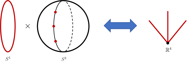
Figure 1: The line operators wrapping $S^{1}$ and inserted along a great circle in $S^{3}$ (left). The rays emanating from the origin in $\mathbb{R}^{4}$ (right). Since they map to one another under the conformal map, the Schur line defect correlators will count the BPS local operators living at a junction of lines.

2.2 Line defect Schur correlators

For $\mathcal{N}=4$ $U(N)$ SYM theory the flavored Schur correlation function of the $k$ half-BPS Wilson line operators $W_{\mathcal{R}_{j}}$, $j=1,\cdots,k$ transforming as the representation $\mathcal{R}_{j}$ under the gauge group $U(N)$ can be evaluated from a matrix integral Gang:2012yr

$$\langle W_{\mathcal{R}_{1}}\cdots W_{\mathcal{R}_{k}}\rangle^{U(N)}(t;q)$$

$$=\frac{1}{N!}\frac{(q;q)_{\infty}^{2N}}{(q^{\frac{1}{2}}t^{\pm 2};q)_{\infty}^{N}}\oint\prod_{i=1}^{N}\frac{d\sigma_{i}}{2\pi i\sigma_{i}}\frac{\prod_{i\neq j}\left(\frac{\sigma_{i}}{\sigma_{j}};q\right)_{\infty}\left(q\frac{\sigma_{i}}{\sigma_{j}};q\right)_{\infty}}{\prod_{i\neq j}\left(q^{\frac{1}{2}}t^{2}\frac{\sigma_{i}}{\sigma_{j}};q\right)_{\infty}\left(q^{\frac{1}{2}}t^{-2}\frac{\sigma_{i}}{\sigma_{j}};q\right)_{\infty}}\prod_{j=1}^{k}\chi_{\mathcal{R}_{j}}(\sigma),$$ (1)

where the integration contour is chosen as a unit torus $\mathbb{T}^{N}$. It is a formal Taylor series in $q^{1/2}$ and its coefficients are Laurent polynomial in $t$ with integer coefficients. Here $\chi_{\mathcal{R}_{j}}(\sigma)$ is a character of the representation $\mathcal{R}_{j}$. Physically, it corresponds to the classical value of the BPS Wilson line operator whose holonomy matrix is specified by gauge fields along the $S^{1}$. We have used a shorthand notation $(q^{\frac{1}{2}}t^{\pm 2};q)_{\infty}=(q^{\frac{1}{2}}t^{2};q)_{\infty}(q^{\frac{1}{2}}t^{-2};q)_{\infty}$. The correlation function (2.2) is obviously invariant under the transformation

$$t \rightarrow t^{-1},$$ (2)

under which two $SU(2)$ subgroups of the $SU(4)$ R-symmetry are swapped. In the absence of the line operators, the flavored Schur line defect correlator (2.2) reduces the flavored Schur index $\mathcal{I}^{U(N)}$. The exact closed-form of the flavored Schur index is explored in Hatsuda:2022xdv .

2.3 Symmetric functions

The characters of the representations under the gauge group appearing in the matrix integral (2.2) is presented as certain symmetric functions in gauge fugacities $\sigma_{i}$.

The Wilson line operator $W_{n}$ with charge $n\in\mathbb{Z}$ in $U(N)$ SYM theory is specified by the character given by the $n$-th power sum symmetric function in $N$ variables

$$p_{n}(\sigma) =\sum_{i=1}^{N}\sigma_{i}^{n}.$$ (3)

The generating function for the Wilson line operators $W_{n}$ with charge $n$ is

$$P(s;\sigma) =\sum_{n=1}^{\infty}p_{n}(\sigma)s^{n}=\sum_{i=1}^{N}\frac{s}{1-s\sigma_{i}}=s\frac{\partial}{\partial s}\log\frac{1}{\prod_{i=1}^{N}(1-s\sigma_{i})}.$$ (4)

The Wilson line operator $W_{(1^{k})}$ in the rank-$k$ antisymmetric representation is described by the character given by the $k$-th elementary symmetric function

$$e_{k}(\sigma) =\sum_{1\leq i_{1}<i_{2}<\cdots<i_{k}\leq N}\sigma_{i_{1}}\sigma_{i_{2}}\cdots\sigma_{i_{k}}.$$ (5)

The generating function for the Wilson line operators $W_{(1^{k})}$ in the antisymmetric representation reads

$$E(s;\sigma) =\sum_{k=0}^{\infty}e_{k}(\sigma)s^{k}=\prod_{i=1}^{N}(1+s\sigma_{i}).$$ (6)

The elementary symmetric function can be expressed as a specialization of the Schur function $s_{\lambda}(\sigma)$

$$e_{k}(\sigma) =s_{(1^{k})}(\sigma).$$ (7)

The Wilson line operator $W_{(k)}$ in the rank-$k$ symmetric representation for $U(N)$ SYM theory is characterized by the complete homogeneous symmetric polynomial of degree $k$ in $N$ variables

$$h_{k}(\sigma) =\sum_{1\leq i_{1}\leq i_{2}\leq\cdots\leq i_{k}\leq N}\sigma_{i_{1}}\sigma_{i_{2}}\cdots\sigma_{i_{k}}.$$ (8)

The generating function for the Wilson line operators $W_{(k)}$ in the symmetric representation is

$$H(s;\sigma) =\sum_{k=0}^{\infty}h_{k}(\sigma)s^{k}=\prod_{i=1}^{N}\frac{1}{1-s\sigma_{i}}.$$ (9)

The complete homogeneous symmetric function can be expressed as a specialization of the Schur function $s_{\lambda}(\sigma)$

$$h_{k}(\sigma) =s_{(k)}(\sigma).$$ (10)

2.3.1 Newton’s identities

Newton’s identities state that

$$ke_{k}(\sigma) =\sum_{i=1}^{k}(-1)^{i-1}e_{k-i}(\sigma)p_{i}(\sigma).$$ (11)

It implies that

$$e_{k}(\sigma) =\sum_{\lambda}(-1)^{k-r}\prod_{i=1}^{r}\frac{1}{\lambda_{i}^{m_{i}}(m_{i}!)}p_{\lambda_{i}}(\sigma)^{m_{i}},$$ (12)

where the sum is taken over all possible partitions $\lambda$ of $k=\sum_{i=1}^{r}\lambda_{i}m_{i}$ with $\lambda_{1}>\lambda_{2}>\cdots>\lambda_{r}$. Similarly, it follows that

$$kh_{k}(\sigma) =\sum_{i=1}^{k}h_{k-i}(\sigma)p_{i}(\sigma).$$ (13)

Hence we have

$$h_{k}(\sigma) =\sum_{\lambda}\prod_{i=1}^{r}\frac{1}{\lambda_{i}^{m_{i}}(m_{i}!)}p_{\lambda_{i}}(\sigma)^{m_{i}}.$$ (14)

As each of families $\{p_{k}(\sigma)\}$, $\{e_{k}(\sigma)\}$ and $\{h_{k}(\sigma)\}$ generates the ring of symmetric polynomials as a polynomial ring. According to the relations (12) and (14), the correlation functions of the Wilson line operators in the rank-$k$ antisymmetric and symmetric representations can be expressed as linear combinations of those of the Wilson lines with fixed charges $n\leq k$.

For example, let us consider the 2-point function of the Wilson line operators in the conjugate representations $\mathcal{R}$ and $\overline{\mathcal{R}}$

$$\langle W_{\mathcal{R}}W_{\overline{\mathcal{R}}}\rangle^{U(N)}$$

$$=\frac{1}{N!}\frac{(q;q)_{\infty}^{2N}}{(q^{\frac{1}{2}}t^{\pm 2};q)_{\infty}^{N}}\oint\prod_{i=1}^{N}\frac{d\sigma_{i}}{2\pi i\sigma_{i}}\frac{\prod_{i\neq j}\left(\frac{\sigma_{i}}{\sigma_{j}};q\right)_{\infty}\left(q\frac{\sigma_{i}}{\sigma_{j}};q\right)_{\infty}}{\prod_{i\neq j}\left(q^{\frac{1}{2}}t^{2}\frac{\sigma_{i}}{\sigma_{j}};q\right)_{\infty}\left(q^{\frac{1}{2}}t^{-2}\frac{\sigma_{i}}{\sigma_{j}};q\right)_{\infty}}\chi_{\mathcal{R}}(\sigma)\chi_{\overline{\mathcal{R}}}(\sigma),$$ (15)

where $\chi_{\overline{\mathcal{R}}}(\sigma)$ $=$ $\chi_{\mathcal{R}}(\sigma^{-1})$. According to the relations (12) and (14) we have

$$\langle W_{(1^{2})}W_{\overline{(1^{2})}}\rangle^{U(N)}$$

$$=\frac{1}{4}\Bigl{[}\langle W_{1}W_{1}W_{-1}W_{-1}\rangle^{U(N)}-2\langle W_{1}W_{1}W_{-2}\rangle^{U(N)}+\langle W_{2}W_{-2}\rangle^{U(N)}\Bigr{]},$$ (16)

$$\langle W_{(2)}W_{\overline{(2)}}\rangle^{U(N)}$$

$$=\frac{1}{4}\Bigl{[}\langle W_{1}W_{1}W_{-1}W_{-1}\rangle^{U(N)}+2\langle W_{1}W_{1}W_{-2}\rangle^{U(N)}+\langle W_{2}W_{-2}\rangle^{U(N)}\Bigr{]}$$ (17)

and

$$\langle W_{(1^{3})}W_{\overline{(1^{3})}}\rangle^{U(N)}$$

$$=\frac{1}{36}\Biggl{[}\langle W_{1}W_{1}W_{1}W_{-1}W_{-1}W_{-1}\rangle^{U(N)}-6\langle W_{1}W_{1}W_{1}W_{-1}W_{-2}\rangle^{U(N)}+4\langle W_{1}W_{1}W_{1}W_{-3}\rangle^{U(N)}$$

$$+9\langle W_{1}W_{2}W_{-1}W_{-2}\rangle^{U(N)}-12\langle W_{1}W_{1}W_{2}W_{-3}\rangle^{U(N)}+\langle W_{3}W_{-3}\rangle^{U(N)}\Biggr{]},$$ (18)

$$\langle W_{(3)}W_{\overline{(3)}}\rangle^{U(N)}$$

$$=\frac{1}{36}\Biggl{[}\langle W_{1}W_{1}W_{1}W_{-1}W_{-1}W_{-1}\rangle^{U(N)}+6\langle W_{1}W_{1}W_{1}W_{-1}W_{-2}\rangle^{U(N)}+4\langle W_{1}W_{1}W_{1}W_{-3}\rangle^{U(N)}$$

$$+9\langle W_{1}W_{2}W_{-1}W_{-2}\rangle^{U(N)}+12\langle W_{1}W_{1}W_{2}W_{-3}\rangle^{U(N)}+\langle W_{3}W_{-3}\rangle^{U(N)}\Biggr{]}.$$ (19)

2.3.2 Irreducible power sum symmetric functions

Let $\lambda=(\lambda_{1},\lambda_{2},\cdots,\lambda_{r})$ be a partition of weight $|\lambda|$ and $I=\{1,2,\cdots,k-1\}$ a set of integers. Given the partition $\lambda$ and the set $I$ we consider a decomposition $I=\bigoplus_{i=1}^{r}I_{i}$ with the conditions $I_{i}\cap I_{j}=\emptyset$ and $|I_{i}|=\lambda_{i}$. We then recursively define irreducible elements of products of $k$ power sum symmetric functions $p_{n_{1}},\cdots,p_{n_{k-1}},p_{-n_{1}-\cdots-n_{k-1}}$ by

$$\mathfrak{p}_{\{n_{1},\cdots,n_{k-1},-n_{1}-\cdots-n_{k-1}\}}$$

$$:=p_{n_{1}}p_{n_{2}}\cdots p_{n_{k-1}}p_{-n_{1}-n_{2}-\cdots-n_{k-1}}$$

$$-\sum_{j=1}^{k-1}\sum_{\begin{smallmatrix}\lambda=(\lambda_{1},\cdots,\lambda_{r})\\ |\lambda|=j,\\ r\leq k-2\\ \end{smallmatrix}}\sum_{\{I_{1},\cdots,I_{r}\}}\mathfrak{p}_{\left\{\sum_{i^{(1)}\in I_{1}}n_{i^{(1)}},\cdots\sum_{i^{(r)}\in I_{r}}n_{i^{(r)}},-\sum_{\alpha=1}^{r}\sum_{i^{(\alpha)}\in I_{\alpha}}n_{i^{(\alpha)}}\right\}}.$$ (20)

Here the sum $\sum_{\{I_{1},\cdots,I_{r}\}}$ is taken over all the possible combinations of subsets of integers. For example, we have

$$\mathfrak{p}_{\{n_{1},-n_{1}\}}=p_{n_{1}}p_{-n_{1}},$$ (21)

$$\mathfrak{p}_{\{n_{1},n_{2},-n_{1}-n_{2}\}}=p_{n_{1}}p_{n_{2}}p_{-n_{1}-n_{2}}-\mathfrak{p}_{\{n_{1},-n_{1}\}}-\mathfrak{p}_{\{n_{2},-n_{2}\}}-\mathfrak{p}_{\{n_{1}+n_{2},-n_{1}-n_{2}\}},$$ (22)

$$\mathfrak{p}_{\{n_{1},n_{2},n_{3},-n_{1}-n_{2}-n_{3}\}}=p_{n_{1}}p_{n_{2}}p_{n_{3}}p_{-n_{1}-n_{2}-n_{3}}-\mathfrak{p}_{\{n_{1},-n_{1}\}}-\mathfrak{p}_{\{n_{2},-n_{2}\}}-\mathfrak{p}_{\{n_{3},-n_{3}\}}$$

$$-\mathfrak{p}_{\{n_{1}+n_{2},-n_{1}-n_{2}\}}-\mathfrak{p}_{\{n_{1}+n_{3},-n_{1}-n_{3}\}}-\mathfrak{p}_{\{n_{2}+n_{3},-n_{2}-n_{3}\}}-\mathfrak{p}_{\{n_{1}+n_{2}+n_{3},-n_{1}-n_{2}-n_{3}\}}$$

$$-\mathfrak{p}_{\{n_{1},n_{2},-n_{1}-n_{2}\}}-\mathfrak{p}_{\{n_{1},n_{3},-n_{1}-n_{3}\}}-\mathfrak{p}_{\{n_{2},n_{3},-n_{2}-n_{3}\}}$$

$$-\mathfrak{p}_{\{n_{1},n_{2}+n_{3},-n_{1}-n_{2}-n_{3}\}}-\mathfrak{p}_{\{n_{2},n_{1}+n_{3},-n_{1}-n_{2}-n_{3}\}}-\mathfrak{p}_{\{n_{3},n_{1}+n_{2},-n_{1}-n_{2}-n_{3}\}}.$$ (23)

For $k>N$ the products of power sum symmetric functions corresponding to the $k$-point functions can be decomposed into a sum of products which have at most $N$ power sum symmetric functions corresponding to the 2-, 3-, $\cdots$, $N$-point functions and a constant term. It follows that

$$p_{n_{1}}p_{n_{2}}\cdots p_{n_{k-1}}p_{-n_{1}-n_{2}-\cdots-n_{k-1}}$$

$$=N\sum_{i=1}^{N}(-1)^{N-i}(N-i)!S(k,N-i+1)$$

$$+\sum_{j=1}^{k-1}\sum_{\begin{smallmatrix}\lambda=(\lambda_{1},\cdots,\lambda_{r})\\ |\lambda|=j,\\ r\leq N-1\ \end{smallmatrix}}\sum_{\{I_{1},\cdots,I_{r}\}}\mathfrak{p}_{\{\sum_{i^{(1)}\in I_{1}}n_{i^{(1)}},\cdots,\sum_{i^{(r)}\in I_{r}}n_{i^{(r)}},-\sum_{\alpha=1}^{r}\sum_{i^{(\alpha)}\in I_{\alpha}}n_{i^{(\alpha)}}\}},$$ (24)

where $S(n,k)$ are the Stirling numbers of the second kind. According to the relation (2.3.2), the $k$-point functions of the Wilson line operators in $U(N)$ SYM theory for $k>N$ can be built up from the $2$-, $3$-, $\cdots$, $N$-point functions.

For example, for $N=2$ the partitions with a single row only contribute in the sum. They are $\lambda=(\lambda_{1})=(j)$ with $1\leq j\leq k-1$ and correspond to the 2-point functions. Hence the $k$-point function of the charged Wilson line operators in $U(2)$ SYM theory can be simply decomposed into a sum of the 2-point functions according to the following relation:

$$p_{n_{1}}p_{n_{2}}\cdots p_{n_{k-1}}p_{-n_{1}-n_{2}-\cdots-n_{k-1}}$$

$$=2(-S(k,2)+S(k,1))+\sum_{j=1}^{k-1}p_{n_{j}}p_{-n_{j}}+\sum_{j_{1}<j_{2}}p_{n_{j_{1}}+n_{j_{2}}}p_{-n_{j_{1}}-n_{j_{2}}}$$

$$+\cdots+\sum_{j_{1}<j_{2}<\cdots<j_{k-2}}p_{n_{j_{1}}+n_{j_{2}}+\cdots+n_{j_{k-2}}}p_{-n_{j_{1}}-n_{j_{2}}-\cdots-n_{j_{k-2}}}$$

$$+p_{n_{j_{1}}+n_{j_{2}}+\cdots+n_{j_{k-1}}}p_{-n_{j_{1}}-n_{j_{2}}-\cdots-n_{j_{k-1}}}.$$ (25)

The $k=3,4$ and $5$-point functions of the charged Wilson line operators read

$$\langle W_{n_{1}}W_{n_{2}}W_{-n_{1}-n_{2}}\rangle^{U(2)}$$

$$=-4\mathcal{I}^{U(2)}+\langle W_{n_{1}}W_{-n_{1}}\rangle^{U(2)}+\langle W_{n_{2}}W_{-n_{2}}\rangle^{U(2)}+\langle W_{n_{1}+n_{2}}W_{-n_{1}-n_{2}}\rangle^{U(2)},$$ (26)

$$\langle W_{n_{1}}W_{n_{2}}W_{n_{3}}W_{-n_{1}-n_{2}-n_{3}}\rangle^{U(2)}=-12\mathcal{I}^{U(2)}+\sum_{i=1}^{3}\langle W_{n_{i}}W_{-n_{i}}\rangle^{U(2)}$$

$$+\sum_{i<j}\langle W_{n_{i}+n_{j}}W_{-n_{i}-n_{j}}\rangle^{U(2)}+\langle W_{n_{1}+n_{2}+n_{3}}W_{-n_{1}-n_{2}-n_{3}}\rangle^{U(2)},$$ (27)

$$\langle W_{n_{1}}W_{n_{2}}W_{n_{3}}W_{n_{4}}W_{-n_{1}-n_{2}-n_{3}-n_{4}}\rangle^{U(2)}=-28\mathcal{I}^{U(2)}+\sum_{i=1}^{4}\langle W_{n_{i}}W_{-n_{i}}\rangle^{U(2)}$$

$$+\sum_{i_{1}<i_{2}}\langle W_{n_{i_{1}}+n_{i_{2}}}W_{-n_{i_{1}}-n_{i_{2}}}\rangle^{U(2)}+\sum_{i_{1}<i_{2}<i_{3}}\langle W_{n_{i_{1}}+n_{i_{2}}+n_{i_{3}}}W_{-n_{i_{1}}-n_{i_{2}}-n_{i_{3}}}\rangle^{U(2)}$$

$$+\langle W_{n_{i_{1}}+n_{i_{2}}+n_{i_{3}}+n_{i_{4}}}W_{-n_{i_{1}}-n_{i_{2}}-n_{i_{3}}-n_{i_{4}}}\rangle^{U(2)}.$$ (28)

For $N=3$ the sum is taken over the two types of partitions with $r=1$ and $r=2$, which are $\lambda$ $=$ $(\lambda_{1})$ and $(\lambda_{1},\lambda_{2})$ corresponding to the 2- and 3-point functions respectively. The $k$-point function can be written as a sum of the 2- and 3-point functions by using the following relation:

$$p_{n_{1}}p_{n_{2}}\cdots p_{n_{k-1}}p_{-n_{1}-n_{2}-\cdots-n_{k-1}}$$

$$=3(2S(k,3)-S(k,2)+S(k,1))$$

$$+\sum_{\lambda_{1}=1}^{k-1}\sum_{i_{1}^{(1)}<\cdots<i^{(1)}_{\lambda_{1}}}p_{n_{i_{1}^{(1)}}+n_{i_{2}^{(1)}}+\cdots n_{i_{\lambda_{1}}^{(1)}}}p_{-n_{i_{1}^{(1)}}-n_{i_{2}^{(1)}}-\cdots n_{i_{\lambda_{1}}^{(1)}}}$$

$$+\sum_{j=1}^{k-1}\sum_{\begin{smallmatrix}0<\lambda_{1}\leq\lambda_{2}\\ \lambda_{1}+\lambda_{2}=j\\ \end{smallmatrix}}\sum_{i_{1}^{(1)}<\cdots<i_{\lambda_{1}}^{(1)}}\sum_{i_{1}^{(2)}<\cdots<i_{\lambda_{2}}^{(2)}}\mathfrak{p}_{\{\sum_{a=1}^{\lambda_{1}}n_{i_{a}^{(1)}},\sum_{a=1}^{\lambda_{2}}n_{i_{a}^{(2)}},-\sum_{\alpha=1}^{2}\sum_{a=1}^{\lambda_{\alpha}}n_{i_{a}^{(\alpha)}},\}}.$$ (29)

For $k=4$ one finds that

$$\langle W_{n_{1}}W_{n_{2}}W_{n_{3}}W_{-n_{1}-n_{2}-n_{3}}\rangle^{U(3)}$$

$$=18\mathcal{I}^{U(3)}+\sum_{i=1}^{2}\langle W_{n_{i}}W_{-n_{i}}\rangle^{U(3)}+\sum_{i<j}\langle W_{n_{i}+n_{j}}W_{-n_{i}-n_{j}}\rangle^{U(3)}+\langle W_{n_{1}+n_{2}+n_{3}}W_{-n_{1}-n_{2}-n_{3}}\rangle^{U(3)}$$

$$+\sum_{i<j}\langle\mathfrak{W}_{n_{i}}\mathfrak{W}_{n_{j}}\mathfrak{W}_{-n_{i}-n_{j}}\rangle^{U(3)}+\sum_{i=1}^{3}\sum_{\begin{smallmatrix}j_{1}\neq i,j_{2}\neq i\\ j_{1}<j_{2}\\ \end{smallmatrix}}\langle\mathfrak{W}_{n_{i}}\mathfrak{W}_{n_{j_{1}}+n_{j_{2}}}\mathfrak{W}_{-n_{1}-n_{2}-n_{3}}\rangle^{U(3)},$$ (30)

where

$$\langle\mathfrak{W}_{n_{1}}\mathfrak{W}_{n_{2}}\mathfrak{W}_{-n_{1}-n_{2}}\rangle^{U(N)}$$

$$:=\langle W_{n_{1}}W_{n_{2}}W_{-n_{1}-n_{2}}\rangle^{U(N)}-\sum_{i=1}^{2}\langle W_{n_{i}}W_{-n_{i}}\rangle^{U(N)}-\langle W_{n_{1}+n_{2}}W_{-n_{1}-n_{2}}\rangle^{U(N)}$$ (31)

is the irreducible part of the 3-point function. The numerical coefficient of the $U(3)$ Schur index in (2.3.2) is computed from the relation (2.3.2) as $3(2S(4,3)-S(4,2)+S(4,1))=18$. For $k=5$ we have

$$\langle W_{n_{1}}W_{n_{2}}W_{n_{3}}W_{n_{4}}W_{-n_{1}-n_{2}-n_{3}-n_{4}}\rangle^{U(3)}$$

$$=108\mathcal{I}^{U(3)}+\sum_{i=1}^{4}\langle W_{n_{i}}W_{-n_{i}}\rangle^{U(3)}+\sum_{i_{1}<i_{2}}\langle W_{n_{i_{1}}+n_{i_{2}}}W_{-n_{i_{1}}-n_{i_{2}}}\rangle^{U(3)}$$

$$+\sum_{i_{1}<i_{2}<i_{3}}\langle W_{n_{i_{1}}+n_{i_{2}}+n_{i_{3}}}W_{-n_{i_{1}}-n_{i_{2}}-n_{i_{3}}}\rangle^{U(3)}+\langle W_{n_{i_{1}}+n_{i_{2}}+n_{i_{3}}+n_{i_{4}}}W_{-n_{i_{1}}-n_{i_{2}}-n_{i_{3}}-n_{i_{4}}}\rangle^{U(3)}$$

$$+\sum_{i_{1}<i_{2}}\langle\mathfrak{W}_{n_{i_{1}}}\mathfrak{W}_{n_{i_{2}}}\mathfrak{W}_{-n_{i_{1}}-n_{i_{2}}}\rangle^{U(3)}+\sum_{i=1}^{4}\sum_{\begin{smallmatrix}i_{2}<i_{3}\\ i_{2}\neq i_{1}\\ i_{3}\neq i_{1}\\ \end{smallmatrix}}\langle\mathfrak{W}_{n_{i_{1}}}\mathfrak{W}_{n_{i_{2}}+n_{i_{3}}}\mathfrak{W}_{-n_{i_{1}}-n_{i_{2}}-n_{i_{3}}}\rangle^{U(3)}$$

$$+\sum_{i=1}^{4}\langle\mathfrak{W}_{n_{i}}\mathfrak{W}_{n_{1}+n_{2}+n_{3}+n_{4}-n_{i}}\mathfrak{W}_{-n_{2}-n_{2}-n_{3}-n_{4}}\rangle^{U(3)}$$

$$+\sum_{i_{1}<i_{2}}\langle\mathfrak{W}_{n_{i_{1}}+n_{i_{2}}}\mathfrak{W}_{n_{1}+n_{2}+n_{3}+n_{4}-n_{i_{1}}-n_{i_{2}}}\mathfrak{W}_{-n_{2}-n_{2}-n_{3}-n_{4}}\rangle^{U(3)}.$$ (32)

Again the numerical coefficient of the $U(3)$ Schur index is fixed from (2.3.2) as $3(2S(5,3)-S(5,2)+S(5,1))$ $=$ $108$.

2.4 Half-BPS limits

When we keep $\mathfrak{q}$ $:=$ $q^{1/2}t^{2}$ fixed and take $q$ to zero, the Schur index reduces to the half-BPS index. In this limit the matrix integral (2.2) reduces to

$$\langle W_{\mathcal{R}_{1}}\cdots W_{\mathcal{R}_{k}}\rangle^{U(N)}_{\textrm{$\frac{1}{2}$BPS}}(\mathfrak{q})=\frac{1}{N!}\oint\prod_{i=1}^{N}\frac{d\sigma_{i}}{2\pi i\sigma_{i}}\frac{\prod_{i\neq j}\left(1-\frac{\sigma_{i}}{\sigma_{j}}\right)}{\prod_{i,j}\left(1-\mathfrak{q}\frac{\sigma_{i}}{\sigma_{j}}\right)}\prod_{j=1}^{k}\chi_{\mathcal{R}_{j}}(\sigma).$$ (33)

The resulting integral (33) defines an inner product of the symmetric functions

$$\langle f,g\rangle :=\frac{1}{N!}\oint\prod_{i=1}^{N}\frac{d\sigma_{i}}{2\pi i\sigma_{i}}\frac{\prod_{i\neq j}\left(1-\frac{\sigma_{i}}{\sigma_{j}}\right)}{\prod_{i,j}\left(1-\mathfrak{q}\frac{\sigma_{i}}{\sigma_{j}}\right)}f(\sigma)g(\sigma^{-1}).$$ (34)

It can be viewed as a $q$-deformation of the Hall inner product. With respect to the inner product (34) the Hall-Littlewood functions $P_{\lambda}(\sigma;\mathfrak{q})$ are orthogonal

$$\langle P_{\lambda}(\sigma;\mathfrak{q}),P_{\mu}(\sigma^{-1},\mathfrak{q})\rangle =\frac{1}{v_{\lambda}}\delta_{\lambda\mu},$$ (35)

where

$$v_{\lambda} =\frac{(\mathfrak{q};\mathfrak{q})_{N-l(\lambda)}\prod_{j\geq 1}(\mathfrak{q};\mathfrak{q})_{m_{j}(\lambda)}}{(1-\mathfrak{q})^{N}}$$ (36)

and $m_{i}(\lambda)$ is the multiplicity of the integer $i$ in the partition $\lambda$. In the absence of line defects the matrix integral (33) reduces to the half-BPS index

$$\mathcal{I}_{\textrm{$\frac{1}{2}$BPS}}^{U(N)} =\frac{1}{(\mathfrak{q};\mathfrak{q})_{N}}.$$ (37)

Consider the 2-point function of the Wilson line operators where the characters are given by the Schur functions

$$\langle W_{\lambda}W_{\bar{\mu}}\rangle_{\textrm{$\frac{1}{2}$BPS}}^{U(N)} =\frac{1}{N!}\oint\prod_{i=1}^{N}\frac{d\sigma_{i}}{2\pi i\sigma_{i}}\frac{\prod_{i\neq j}\left(1-\frac{\sigma_{i}}{\sigma_{j}}\right)}{\prod_{i,j}\left(1-\mathfrak{q}\frac{\sigma_{i}}{\sigma_{j}}\right)}s_{\lambda}(\sigma)s_{\mu}(\sigma^{-1}).$$ (38)

Since the Schur functions can be decomposed in terms of the Hall-Littlewood functions

$$s_{\lambda}(\sigma) =\sum_{\nu}K_{\lambda\nu}(\mathfrak{q})P_{\nu}(\sigma;\mathfrak{q}),$$ (39)

where $K_{\lambda\nu}(\mathfrak{q})$ is the Kostka-Foulkes polynomial MR1354144 , the matrix integral can be formally evaluated from (35) as

$$\langle W_{\lambda}W_{\bar{\mu}}\rangle_{\textrm{$\frac{1}{2}$BPS}}^{U(N)} =\sum_{\nu}\frac{K_{\lambda\nu}(\mathfrak{q})K_{\mu\nu}(\mathfrak{q})}{\prod_{n=1}^{N-l(\nu)}(1-\mathfrak{q}^{n})\prod_{j\geq 1}\prod_{n=1}^{m_{j}(\nu)}(1-\mathfrak{q}^{n})}.$$ (40)

3 Fermi-gas formulation

In Hatsuda:2022xdv the closed-form expressions for the Schur index of $\mathcal{N}=2^{*}$ $U(N)$ SYM theory are presented by means of the Fermi-gas method. In this section we extend the analysis to the Schur line defect correlation functions.

We redefine the flavor fugacity by replacing $t$ with $\xi=q^{-1/2}t^{2}=e^{2\pi i\zeta}$ which is associated with the $\mathcal{N}=2^{*}$ deformation due to the mass parameter for the adjoint hypermultiplet. We define a new function

$$\theta(x;q) :=\sum_{n\in\mathbb{Z}}(-1)^{n}x^{n+\frac{1}{2}}q^{\frac{n^{2}+n}{2}}$$

$$=(x^{\frac{1}{2}}-x^{-\frac{1}{2}})\prod_{n=1}^{\infty}(1-q^{n})(1-xq^{n})(1-x^{-1}q^{n}).$$ (41)

Then the matrix integral (2.2) can be rewritten as

$$\langle W_{\mathcal{R}_{1}}\cdots W_{\mathcal{R}_{k}}\rangle^{U(N)}(\xi;q)$$

$$=\frac{(-1)^{N}\xi^{N^{2}/2}}{N!}\oint_{|\sigma_{i}|=1}\prod_{i=1}^{N}\frac{d\sigma_{i}}{2\pi i\sigma_{i}}\frac{\theta^{\prime}(1;q)^{N}\prod_{i<j}\theta(\frac{\sigma_{i}}{\sigma_{j}};q)\theta(\frac{\sigma_{i}}{\sigma_{j}}:q)}{\prod_{i,j}\theta(\frac{\sigma_{i}}{\sigma_{j}}\xi^{-2};q)}\prod_{j=1}^{k}\chi_{\mathcal{R}_{j}}(\sigma).$$ (42)

Corresponding to (2), the integral (3) is invariant under

$$\xi \rightarrow q^{-1}\xi^{-1}.$$ (43)

According to the Frobenius determinant formula Frobenius:1882uber ; MR0335789 ; Mason:2008zzb

$$\frac{(q;q)_{\infty}^{3N}\prod_{i<j}\theta(v_{i}v_{j}^{-1};q)\theta(w_{j}w_{i}^{-1};q)}{\prod_{i,j}\theta(v_{i}w_{j}^{-1};q)} =\frac{\theta(u;q)}{\theta(u\prod_{i}v_{i}w_{i}^{-1};q)}\det_{i,j}F(v_{i}w_{j}^{-1},u;q),$$ (44)

where

$$F(x,y;q) :=\frac{\theta(xy;q)(q;q)_{\infty}^{3}}{\theta(x;q)\theta(y;q)}$$ (45)

is the Kronecker theta function zbMATH02706826 ; MR1723749 ; MR1106744 ; MR2796409 , one can express (3) as

$$\langle W_{\mathcal{R}_{1}}\cdots W_{\mathcal{R}_{k}}\rangle^{U(N)}(\xi;q)$$

$$=\frac{(-1)^{N}\xi^{N^{2}/2}}{N!}\frac{\theta(u;q)}{\theta(u\xi^{-N};q)}\oint_{|\sigma_{i}|=1}\prod_{i=1}^{N}\frac{d\sigma_{i}}{2\pi i\sigma_{i}}\det_{i,j}F\left(\frac{\sigma_{i}}{\sigma_{j}}\xi^{-1},u;q\right)\prod_{j=1}^{k}\chi_{\mathcal{R}_{j}}(\sigma).$$ (46)

In the absence of the characters $\chi_{\mathcal{R}_{j}}$ in the integrand of (2.2) it reduces to the Schur index and the normalized function

$$\mathcal{Z}(N;u;\xi;q) =\frac{1}{N!}\oint_{|\sigma_{i}|=1}\prod_{i=1}^{N}\frac{d\sigma_{i}}{2\pi i\sigma_{i}}\det_{i,j}F\left(\frac{\sigma_{i}}{\sigma_{j}}\xi^{-1},u;q\right)$$ (47)

can be regarded as a partition function of free Fermi-gas with $N$ particles on a circle which is characterized by a one-particle density matrix

$$\rho_{0}(\alpha,\alpha^{\prime};u;\xi;q) =F(e^{2\pi i(\alpha-\alpha^{\prime})}\xi^{-1},u;\xi;q)$$

$$=-\sum_{p\in\mathbb{Z}}\frac{e^{2\pi ip(\alpha-\alpha^{\prime})}\xi^{-p}}{1-uq^{p}},$$ (48)

where $0\leq$ $\alpha$ $=\frac{1}{2\pi i}\log\sigma$ $\leq 1$ is the periodic position operator and $p$ is the discrete momentum operator.

In order to generalize the Fermi-gas method to the Schur line defect correlation functions, we use the idea in Hatsuda:2013yua ; Drukker:2015spa . We consider matrix integrals

$$\mathcal{Z}_{E}^{\{n_{j}\}}(N;\{s_{j}\};u;\xi;q) =\frac{1}{N!}\oint_{|\sigma_{i}|=1}\prod_{i=1}^{N}\frac{d\sigma_{i}}{2\pi i\sigma_{i}}\det_{i,j}F\left(\frac{\sigma_{i}}{\sigma_{j}}\xi^{-1},u;q\right)\prod_{j=1}^{k}E(s_{j};\sigma^{n_{j}})$$ (49)

and

$$\mathcal{Z}_{H}^{\{n_{j}\}}(N;\{s_{j}\};u;\xi;q) =\frac{1}{N!}\oint_{|\sigma_{i}|=1}\prod_{i=1}^{N}\frac{d\sigma_{i}}{2\pi i\sigma_{i}}\det_{i,j}F\left(\frac{\sigma_{i}}{\sigma_{j}}\xi^{-1},u;q\right)\prod_{j=1}^{k}H(s_{j};\sigma^{n_{j}}),$$ (50)

where $E(s_{j};\sigma)$ and $H(s_{j};\sigma)$ are the generating functions (6) and (9) for the characters of the antisymmetric representations and those of the symmetric representations. These matrix integrals play a role of generating functions for the correlation functions of the Wilson line operators. For example, the correlation functions of the Wilson line operators $W_{n_{j}}$ of charges $\{n_{j}\}_{j=1}^{k}$ can be obtained from the coefficient of the term with $\prod_{j=1}^{k}s_{j}$ in either of (49) or (50). Besides, for $k=2$ and $(n_{1},n_{2})=(1,-1)$ one can extract the 2-point functions of the Wilson line operators $W_{(1^{l})}$ (resp. $W_{(l,0)}$) in the rank-$l$ antisymmetric representations (resp. symmetric representations) by reading off the term including $s_{1}^{l}s_{2}^{l}$ in (49) (resp. in (50)).

We observe that the introductions of the products $\prod_{j=1}^{k}$ $\prod_{i=1}^{N}$ $E(s_{j};\sigma^{n_{j}})$ in (49) and $\prod_{j=1}^{k}$ $\prod_{i=1}^{N}$ $H(s_{j};\sigma^{n_{j}})$ in (50) replace the density matrix (3) with

$$\rho_{E}^{(n_{1},n_{2},\cdots,n_{k})}(\{s_{j}\};\alpha,\alpha^{\prime};u,\xi;q) =X_{E}^{(n_{1},n_{2},\cdots,n_{k})}(\{s_{j}\};\alpha)\rho_{0}(\alpha,\alpha^{\prime};u,\xi;q)$$ (51)

and

$$\rho_{H}^{(n_{1},n_{2},\cdots,n_{k})}(\{s_{j}\};\alpha,\alpha^{\prime};u,\xi;q) =X_{H}^{(n_{1},n_{2},\cdots,n_{k})}(\{s_{j}\};\alpha)\rho_{0}(\alpha,\alpha^{\prime};u,\xi;q),$$ (52)

where we have defined position-dependent matrices

$$X_{E}^{(n_{1},n_{2},\cdots,n_{k})}(\{s_{j}\};\alpha) =\prod_{j=1}^{k}E(s_{j};e^{2\pi in_{j}\alpha}).$$ (53)

and

$$X_{H}^{(n_{1},n_{2},\cdots,n_{k})}(\{s_{j}\};\alpha) =\prod_{j=1}^{k}H(s_{j};e^{2\pi in_{j}\alpha}).$$ (54)

In other words, the matrix integrals (49) and (50) are now identified with the canonical partition functions of free Fermi-gas with $N$ particles whose density matrices are given by (51) and (52).

3.1 Spectral zeta functions

3.1.1 Multiple Kronecker theta series

We define a function

$$Q(\{l_{i}\};\{n_{i}\};u;\xi;q) :=\sum_{p\in\mathbb{Z}}\prod_{i=0}^{k}\frac{(-1)^{l_{i}}\xi^{-l_{i}p-l_{i}n_{i}}}{(1-uq^{p+n_{i}})^{l_{i}}},$$ (55)

where $n_{0}=0$. As this function generalizes the Fourier series (3) of the Kronecker theta function by including mult-index obeying certain condition, we call the function (55) multiple Kronecker theta series.

The multiple Kronecker theta series (55) plays a role of elementary blocks of the Schur indices and line defect correlators. If $k=0$ and $l_{0}=l$, the multiple Kronecker theta series (55) becomes the spectral zeta function associated with the density matrix $\rho_{0}$ of the Fermi-gas for the Schur index of $\mathcal{N}=2^{*}$ $U(N)$ SYM theory Hatsuda:2022xdv

$$Z_{l}(u;\xi;q) :=\mathrm{Tr}(\rho_{0}^{l})$$

$$=Q(l;0;u;\xi;q)=\sum_{p\in\mathbb{Z}}\left(\frac{-\xi^{-p}}{1-uq^{p}}\right)^{l}.$$ (56)

We can write the spectral zeta function for $l=1$ as

$$Z_{1}(u;\xi;q) =\frac{(q)_{\infty}^{3}\theta(\xi^{-1}u)}{\theta(\xi^{-1})\theta(u)}=P_{1}\left[\begin{matrix}\xi\\ 1\\ \end{matrix}\right](\nu,\tau)$$ (57)

and

$$Z_{l}(u;\xi;q) =\frac{u^{-(l-1)}}{(l-1)!}\sum_{k=1}^{l-1}k!|s(l-1,k)|P_{k+1}\left[\begin{matrix}q^{l-1}\xi^{l}\\ 1\\ \end{matrix}\right](\nu,\tau)$$ (58)

for $l\geq 2$ with $u=e^{2\pi i\nu}$ and $q=e^{2\pi i\tau}$. Here $s(n,k)$ are the Stirling numbers of the first kind and

$$P_{k}\left[\begin{matrix}\theta\\ \phi\\ \end{matrix}\right](z,\tau) =\frac{(-1)^{k}}{(k-1)!}{\sum_{n\in\mathbb{Z}}}^{\prime}\frac{(n+\lambda)^{k-1}x^{n+\lambda}}{1-\theta^{-1}q^{n+\lambda}}$$ (59)

is the twisted Weierstrass function Mason:2008zzb where $\sum^{\prime}$ stands for the sum that omits $n=0$ if $(\theta,\phi)=(1,1)$.

In Hatsuda:2022xdv it is shown that the Schur indices of $\mathcal{N}=2^{*}$ $U(N)$ SYM theories can be expressible in terms of the spectral zeta functions (3.1.1).

More generally, the multiple Kronecker theta series (55) can be written in terms of the twisted Weierstrass function by means of the partial expansion into the function (3.1.1). It is convenient to define functions

$$(n)_{q,\xi} :=-\frac{\xi^{-n}}{1-q^{n}}=\frac{q^{-\frac{n}{2}}\xi^{-n}}{q^{\frac{n}{2}}-q^{-\frac{n}{2}}},$$ (60)

$$[n]_{q} :=\frac{1-q^{n}}{1-q}.$$ (61)

The function (60) transforms as

$$(n)_{q,q^{-1}\xi^{-1}} =-(-n)_{q,\xi}$$

$$=q^{n}\xi^{2n}(n)_{q,\xi}$$ (62)

under (43). It follows that

$$[n]_{q} =\frac{(1)_{q,1}}{(n)_{q,1}},$$ (63)

$$(n)_{q,\xi}+(-n)_{q,\xi} =-\frac{(n)_{q,\xi}}{(n)_{q\xi^{2},1}}=-\frac{q^{\frac{n}{2}}\xi^{n}-q^{-\frac{n}{2}}\xi^{-n}}{q^{\frac{n}{2}}-q^{-\frac{n}{2}}},$$ (64)

$$\frac{(n)_{q,\xi}^{2}}{(n)_{q\xi,1}}+\frac{(-n)_{q,\xi}^{2}}{(-n)_{q\xi,1}} =-\frac{(n)_{q,\xi}^{2}}{(n)_{q\xi,1}(n)_{q\xi^{3},1}},$$ (65)

where

$$\frac{1}{(n)_{q\xi^{2},1}} =q^{\frac{n}{2}}\xi^{n}(q^{\frac{n}{2}}\xi^{n}-q^{-\frac{n}{2}}\xi^{-n}).$$ (66)

These relations are useful to describe the correlation functions.

Let $l_{\max}$ be the maximal value of the integers $\{l_{i}\}$, $i=0,\cdots,k$ for the function $Q(\{l_{i}\};\{n_{i}\};u;\xi;q)$. For $k>0$ the function $Q(\{l_{i}\};\{n_{i}\};u;\xi;q)$ can be decomposed into $\sum_{i}l_{i}$ parts, each of which is expressed in terms of the spectral zeta function $Q(l;0;u;\xi;q)=Z_{l}(u;\xi;q)$ with $1\leq l\leq l_{\max}$ and the function (60).

For example, for $k=1$ we have

$$Q(l_{0},l_{1};0,n;u;\xi;q)$$

$$=\sum_{k=0}^{l_{0}-1}\left(\begin{matrix}k+l_{1}-1\\ l_{1}-1\\ \end{matrix}\right)(-1)^{k}q^{kn}\xi^{kn}(n)_{q,\xi}^{k+l_{1}}Q(l_{0}-k;0;\xi^{\frac{l_{0}+l_{1}}{l_{0}-k}};q)$$

$$+\sum_{k=0}^{l_{1}-1}\left(\begin{matrix}k+l_{0}-1\\ k\\ \end{matrix}\right)(-1)^{k}q^{-kn}\xi^{-kn}(-n)_{q,\xi}^{k+l_{0}}Q(l_{1}-k;0;u;\xi^{\frac{l_{0}+l_{1}}{l_{1}-k}};q).$$ (67)

Clearly, it follows that

$$Q(l_{1},l_{0};0,n;u;\xi;q) =Q(l_{0},l_{1};0,-n,u;\xi;q).$$ (68)

Several examples are shown in Appendix B.

For $k=2$ with $l_{0}=l$, $l_{1}=l_{2}=1$ one finds that

$$Q(l,1,1;0,n_{1},n_{2};u;\xi;q)$$

$$=\sum_{m=1}^{l}\sum_{k=0}^{m-1}\sum_{k_{1}+k_{2}=k}\left(\begin{matrix}m\\ k+1\\ \end{matrix}\right)(-1)^{k+m-1}q^{(m-1)(n_{1}+n_{2})-k_{1}n_{1}-k_{2}n_{2}}\xi^{(m-1)(n_{1}+n_{2})}$$

$$\times(n_{1})_{q,\xi}^{m}(n_{2})_{q,\xi}^{m}Q(l-m+1;0;u;\xi^{\frac{l+2}{l-m+1}};q)$$

$$+(-n_{1})_{q,\xi}^{l}(-n_{1}+n_{2})_{q,\xi}Q(1;0;u;\xi^{l+2};q)$$

$$+(-n_{2})_{q,\xi}^{l}(-n_{2}+n_{1})_{q,\xi}Q(1;0;u;\xi^{l+2};q).$$ (69)

We have

$$Q(1,l,1;0,n_{1},n_{2};u;\xi;q) =Q(l,1,1;0,-n_{1},n_{2}-n_{1};u;\xi;q),$$ (70)

$$Q(1,1,l;0,n_{1},n_{2};u;\xi;q) =Q(l,1,1;0,n_{1}-n_{2},-n_{2};u;\xi;q).$$ (71)

Further examples for $k=2$ are found in Appendix B.2.

For general $k$ with $l_{0}=l_{1}=\cdots=l_{k}=1$ the multiple Kronecker theta series (55) can be decomposed as

$$Q(1,\cdots,1;0,n_{1},\cdots,n_{k};u;\xi;q)$$

$$=\Bigl{[}\prod_{i=1}^{k}(n_{i})_{q,\xi}+\sum_{i=1}^{k}\sum_{j\neq i}(-n_{i})_{q,\xi}(-n_{i}+n_{j})_{q,\xi}\Bigr{]}Q(1;0;u;\xi^{k+1};q).$$ (72)

Likewise, the spectral zeta functions for the modified density matrices (51) and (52) can be expressed in terms of the multiple Kronecker theta series (55). Noting that $\sigma=e^{2\pi i\alpha}$ is a translation operator

$$\sigma^{-n}\mathcal{O}(p)\sigma^{n} =e^{-2\pi in\alpha}\mathcal{O}(p)e^{2\pi in\alpha}=\mathcal{O}(p+n),$$ (73)

where $\mathcal{O}(p)$ is some $p$-dependent operator, the spectral zeta functions can be calculated by taking traces of normal ordered operators $(X_{E/H}^{(n_{1},n_{2},\cdots,n_{k})}(\alpha)\rho(p))^{l}$.

We obtain the spectral zeta function associated with the modified density matrix (51) of the form

$$Z_{l}^{E}(n_{1},n_{2},\cdots,n_{k-1})=\mathrm{Tr}\left({\rho_{E}^{(n_{1},n_{2},\cdots,n_{k})}}^{l}\right)$$

$$=Z_{l}(u;\xi;q)+Z_{l;1}^{(k-1)}(\{n_{i}\};u;\xi;q)\prod_{i=1}^{k}s_{i}+\prod_{m\geq 2}Z_{l;m}^{E;(k-1)}(\{n_{i}\};u;\xi;q)\prod_{i=1}^{k}s_{i}^{m},$$ (74)

where $Z_{l}(u;\xi;q)$ $=$ $Q(l;0;u;\xi;q)$ which is independent of the fugacities $\{s_{i}\}$ encodes the Schur index without any insertion of the line operators. It is nothing but the spectral zeta function (3.1.1) for the density matrix $\rho_{0}$. The function $Z_{l;1}^{(k-1)}$ which appears in the terms with $\prod_{i}s_{i}$ captures the $k$-point functions of the charged Wilson line operators. It is given by

$$Z^{(k-1)}_{l;1}(\{n_{i}\};u;\xi;q)=l\sum_{j=1}^{k}\sum_{l_{1}+\cdots l_{j}=l}\sum_{\{N_{J_{i}}\}_{i=1}^{j}}Q\left(\{l_{i}\}_{i=1}^{j};\{N_{J_{i}}\}_{i=1}^{j};u;\xi;q\right),$$ (75)

where

$$N_{J_{i}} =\sum_{a_{*}\in J_{i}}n_{a_{*}}$$ (76)

and each $J_{i}$ is a subset of integers labeling the charged Wilson line operators obeying the condition

$$\emptyset=J_{1}\subset J_{2}\subset\cdots\subset J_{j}\subseteq I=\{1,2,\cdots,k-1\}.$$ (77)

Here $A\subseteq B$ allows the case $A=B$ while $A\subset B$ excludes it. Since $J_{1}$ is empty, $N_{J_{1}}$ is $0$. For example, when $k>5$ the subsets

$$J_{1}=\emptyset,\qquad J_{2}=\{1,2\},\qquad J_{3}=\{1,2,3,4,5\}$$ (78)

are allowed so that we have

$$N_{J_{1}}=0,\qquad N_{J_{2}}=n_{1}+n_{2},\qquad N_{J_{3}}=n_{1}+n_{2}+n_{3}+n_{4}+n_{5}.$$ (79)

The other terms $Z_{l;m}^{E;(k-1)}(\{n_{j}\};u;\xi;q)$ in (3.1.1) encode the 2-point functions of the Wilson line operators transforming in the rank-$m$ antisymmetric representations. The $k$-point function of $\mathcal{N}=2^{*}$ $U(N)$ SYM theory can be constructed from the spectral zeta functions $Z_{l}^{E}(n_{1},\cdots,n_{k-1})$ with $l=1,\cdots,N$.

Similarly, the spectral zeta function specified by the other modified density matrix (52) takes the form

$$Z_{l}^{H}(n_{1},n_{2},\cdots,n_{k-1})=\mathrm{Tr}\left({\rho_{H}^{(n_{1},n_{2},\cdots,n_{k})}}^{l}\right)$$

$$=Z_{l}(u;\xi;q)+Z_{l;1}^{(k-1)}(\{n_{i}\};u;\xi;q)\prod_{i=1}^{k}s_{i}+\prod_{m\geq 2}Z_{l;m}^{H;(k-1)}(\{n_{i}\};u;\xi;q)\prod_{i=1}^{k}s_{i}^{m}.$$ (80)

Again whereas the function $Z_{l;1}^{(k-1)}$ appears as a coefficient of the terms with $\prod_{j}s_{j}$, the terms $Z_{l;m}^{H;(k-1)}(\{n_{j}\};u;\xi;q)$ encode the 2-point functions of the Wilson line operators transforming in the rank-$m$ symmetric representations.

3.1.2 $Z_{l}^{E}$

We show several examples of the spectral zeta functions. For simplicity we abbreviate $Q(\{l_{i}\};\{n_{i}\};u;\xi;q)=Q(\{l_{i}\};\{n_{i}\})$.

For $k=2$ the spectral zeta functions for the modified density matrix (51) are

$$Z_{1}^{E}(n) =(1+s_{1}s_{2})Q(1;0),$$ (81)

$$Z_{2}^{E}(n) =(1+s_{1}^{2}s_{2}^{2})Q(2;0)+2s_{1}s_{2}\left[Q(2;0)+Q(1,1;0,n)\right],$$ (82)

$$Z_{3}^{E}(n) =(1+s_{1}^{3}s_{2}^{3})Q(3;0)$$

$$+3(s_{1}s_{2}+s_{1}^{2}s_{2}^{2})\Bigl{[}Q(3;0)+Q(2,1;0,n)+Q(1,2;0,n)\Bigr{]},$$ (83)

$$Z_{4}^{E}(n) =(1+s_{1}^{4}s_{2}^{4})Q(4;0)$$

$$+4(s_{1}s_{2}+s_{1}^{3}s_{2}^{3})\Bigl{[}Q(4;0)+Q(3,1;0,n)+Q(2,2;0,n)+Q(1,3;0,n)\Bigr{]}$$

$$+s_{1}^{2}s_{2}^{2}\Bigl{[}6Q(4;0)+8Q(3,1;0,n)+10Q(2,2;0,n)$$

$$+8Q(1,3;0,n)+4Q(1,2,1;0,n,2n)\Bigr{]},$$ (84)

$$Z_{5}^{E}(n) =(1+s_{1}^{5}s_{2}^{5})Q(5;0)$$

$$+5(s_{1}s_{2}+s_{1}^{4}s_{2}^{4})\Bigl{[}Q(5;0)+Q(4,1;0,n)+Q(3,2;0,n)$$

$$+Q(2,3;0,n)+Q(1,4;0,n)\Bigr{]}$$

$$+(s_{1}^{2}s_{2}^{2}+s_{1}^{3}s_{2}^{3})\Bigl{[}10Q(5;0)+15Q(4,1;0,n)+20Q(3,2;0,n)+20Q(2,3;0,n)$$

$$+15Q(1,4;0,n)+5Q(2,2,1;0,n,2n)+10Q(1,3,1;0,n,2n)+5Q(1,2,2;0,n,2n)\Bigr{]}.$$ (85)

These spectral zeta functions with $k=2$ are the blocks of the 2-point functions. In particular, we have

$$Z_{l;1}^{(1)}(n) =lQ(l;0)+l\sum_{k=1}^{l-1}Q(l-k,k;0,n).$$ (86)

For $k=3$ we get

$$Z_{1}^{E}(n_{1},n_{2}) =(1+s_{1}s_{2}s_{3})Q(1;0),$$ (87)

$$Z_{2}^{E}(n_{1},n_{2}) =(1+s_{1}^{2}s_{2}^{2}s_{3}^{2})Q(2;0)+2s_{1}s_{2}s_{3}\Bigl{[}Q(2;0)+Q(1,1;0,n_{1})$$

$$+Q(1,1;0,n_{2})+Q(1,1;0,n_{1}+n_{2})\Bigr{]},$$ (88)

$$Z_{3}^{E}(n_{1},n_{2}) =(1+s_{1}^{3}s_{2}^{3}s_{3}^{3})Q(3;0)$$

$$+3(s_{1}s_{2}s_{3}+s_{1}^{2}s_{2}^{2}s_{3}^{2})\Bigl{[}Q(3;0)+\sum_{i=1}^{2}Q(2,1;0,n_{i})+Q(2,1;0,n_{1}+n_{2})$$

$$+\sum_{i=1}^{2}Q(1,2;0,n_{i})+Q(1,2;0,n_{1}+n_{2})+\sum_{i=1}^{2}Q(1,1,1;0,n_{i},n_{1}+n_{2})\Bigr{]}.$$ (89)

These spectral zeta functions are associated to the 3-point functions. The terms which are associated with $s_{1}s_{2}s_{3}$ describe the 3-point functions of the charged Wilson line operators. They are given by

$$Z_{l;1}^{(2)} =lQ(l;0)+l\Bigl{[}\sum_{k=1}^{l-1}\sum_{i=1}^{2}Q(l-k,k;0,n_{i})+Q(l-k,k;0,n_{1}+n_{2})\Bigr{]}$$

$$+l\sum_{\begin{smallmatrix}0<k_{1},k_{2}\\ 2\leq k_{1}+k_{2}\leq l-1\\ \end{smallmatrix}}\sum_{i=1}^{2}Q(l-k_{1}-k_{2},k_{1},k_{2};0,n_{i},n_{1}+n_{2}).$$ (90)

For $k=4$ we find

$$Z_{1}^{E}(n_{1},n_{2},n_{3}) =(1+s_{1}s_{2}s_{3}s_{4})Q(1;0),$$ (91)

$$Z_{2}^{E}(n_{1},n_{2},n_{3}) =(1+s_{1}^{2}s_{2}^{2}s_{3}^{2}s_{4}^{2})Q(2;0)$$

$$+2s_{1}s_{2}s_{3}s_{4}\Bigl{[}Q(2;0)+Q(1,1;0,n_{1})+Q(1,1;0,n_{2})+Q(1,1;0,n_{3})$$

$$+Q(1,1;0,n_{1}+n_{2})+Q(1,1;0,n_{1}+n_{3})+Q(1,1;0,n_{2}+n_{3})$$

$$+Q(1,1;0,n_{1}+n_{2}+n_{3})\Bigr{]}.$$ (92)

$$Z_{3}^{E}(n_{1},n_{2},n_{3}) =(1+s_{1}^{3}s_{2}^{3}s_{3}^{3}s_{4}^{3})Q(3;0)$$

$$+3(s_{1}s_{2}s_{3}s_{4}+s_{1}^{2}s_{2}^{2}s_{3}^{2}s_{4}^{2})\Bigl{[}Q(3;0)+\sum_{i=1}^{3}Q(2,1;0,n_{i})$$

$$+\sum_{i=1}^{3}\sum_{i<j}Q(2,1;0,n_{i}+n_{j})+Q(2,1;0,n_{1}+n_{2}+n_{3})$$

$$+\sum_{i=1}^{3}Q(1,2;0,n_{i})+\sum_{i<j}Q(1,2;0,n_{i}+n_{j})+Q(1,2;0,n_{1}+n_{2}+n_{3})$$

$$+\sum_{i=1}^{3}\sum_{j\neq i}Q(1,1,1;0,n_{i},n_{i}+n_{j})+\sum_{i=1}^{3}Q(1,1,1;0,n_{i},n_{1}+n_{2}+n_{3})$$

$$+\sum_{i<j}Q(1,1,1;0,n_{i}+n_{j},n_{1}+n_{2}+n_{3})\Bigr{]}.$$ (93)

The 4-point functions of the charged Wilson line operators are captured by

$$Z_{l;1}^{(3)} =lQ(l;0)+l\Bigl{[}\sum_{k=1}^{l-1}\Bigl{\{}\sum_{i=1}^{3}Q(l-k,k;0,n_{i})+\sum_{i<j}Q(l-k,k;0,n_{i}+n_{j})\Bigr{\}}\Bigr{]}$$

$$+l\Bigl{[}\sum_{\begin{smallmatrix}0<k_{1},k_{2}\\ 2\leq k_{1}+k_{2}\leq l-1\\ \end{smallmatrix}}\Bigl{\{}\sum_{i=1}^{3}\sum_{j\neq i}Q(l-k_{1}-k_{2};k_{1},k_{2};0,n_{i},n_{i}+n_{j})$$

$$+\sum_{i=1}^{3}Q(l-k_{1}-k_{2};k_{1},k_{2};0,n_{i},n_{1}+n_{2}+n_{3})$$

$$+\sum_{i<j}Q(l-k_{1}-k_{2},k_{1},k_{2};0,n_{i}+n_{j},n_{1}+n_{2}+n_{3})\Bigr{]}$$

$$+l\sum_{\begin{smallmatrix}0<k_{1},k_{2},k_{3}\\ 3\leq k_{1}+k_{2}+k_{3}\leq l-1\\ \end{smallmatrix}}\sum_{i=1}^{3}\sum_{j\neq i}Q(l-k_{1}-k_{2}-k_{3},k_{1},k_{2},k_{3};0,n_{i},n_{i}+n_{j},n_{1}+n_{2}+n_{3}),$$ (94)

which appears in the terms associated with $s_{1}s_{2}s_{3}s_{4}$.

3.1.3 $Z_{l}^{H}$

The 2-point function of the Wilson line operator in the symmetric representation and that in its conjugate representation can be obtained from $Z_{l}^{H}$ with $k=2$. We find

$$Z_{1}^{H}(n) =\sum_{k=0}^{\infty}s_{1}^{k}s_{2}^{k}Q(1;0),$$ (95)

$$Z_{2}^{H}(n) =\sum_{k=0}^{\infty}s_{1}^{k}s_{2}^{k}\left[(k+1)Q(2;0)+\sum_{l=1}^{k}2(k-l+1)Q(1,1;0,ln)\right],$$ (96)

$$Z_{3}^{H}(n) =\sum_{k=0}^{\infty}s_{1}^{k}s_{2}^{k}\Bigl{[}\frac{(k+1)(k+2)}{2}Q(3;0)$$

$$+\sum_{l=1}^{k}\frac{3(k-l+1)(k-l+2)}{2}\{Q(2,1;0,ln)+Q(1,2;0,ln)\}$$

$$+\sum_{l_{1}=2}\sum_{0<l_{2}<l_{1}}3(k-l_{1}+1)(k-l_{1}+2)Q(1,1,1;0,l_{2},l_{1})\Bigr{]}.$$ (97)

See Appendix C for more examples.

3.2 Closed-form formula

Let $\lambda=(\lambda_{1}^{m_{1}}\lambda_{2}^{m_{2}}\cdots\lambda_{r}^{m_{r}})$ be a partition of integer $N$ with $\sum_{i=1}^{r}m_{i}\lambda_{i}=N$ and $\lambda_{1}>\lambda_{2}$ $>\cdots>$ $\lambda_{r}>\lambda_{r+1}=0$. Then we have

$$\mathcal{Z}_{E/H}^{\{n_{j}\}}(N;\{s_{j}\};u;\xi;q) =\sum_{\lambda}(-1)^{N-r}\prod_{i=1}^{r}\frac{1}{\lambda_{i}^{m_{i}}(m_{i}!)}{Z_{\lambda_{i}}^{E/H}(n_{1},\cdots,n_{k-1})}^{m_{i}}.$$ (98)

Now we can obtain the closed-form expressions for the Schur line defect correlation functions. Since the Schur line defect correlation functions are independent of the variable $u$, it is convenient to fix $u$ to some special value.

When we set $u$ to $\xi^{N/2}$, the canonical partition function of the Fermi-gas is identical to the Schur index up to the overall factor $(-1)^{N+1}\xi^{N^{2}/2}$. Besides, this specialization yields the closed-form expressions for the Schur line defect correlators as multiple series which generalize the nested sum of the Schur index obtained in Hatsuda:2022xdv

$$\mathcal{I}^{U(N)} =-\sum_{\begin{smallmatrix}p_{1},\cdots,p_{N}\in\mathbb{Z}\\ p_{1}<\cdots<p_{N}\\ \end{smallmatrix}}\frac{\xi^{\frac{N^{2}}{2}-\sum_{i=1}p_{i}}}{\prod_{i=1}^{N}(1-\xi^{\frac{N}{2}}q^{p_{i}})}.$$ (99)

It is closely related to the multiple $q$-zeta values ($q$-MVZs) schlesinger2001some ; MR2069738 ; MR2111222 ; MR1992130 ; MR2341851 ; MR2322731 ; MR2843304 ; MR3141529 ; okounkov2014hilbert ; MR3338962 ; MR3473421 ; MR3522085 ; milas2022generalized and $q$-multiple polylogarithms ($q$-MPLs) schlesinger2001some ; MR2341851 ; MR3687119 . We leave more detailed investigation of the relation to these functions to future work.

When we choose $u$ as $\xi$, the multiple Kronecker theta series $Q(1;0;u;\xi;q)$ vanishes

$$Q(1;0;u=\xi) =0,$$ (100)

which can lead to the expression with fewer terms. For simplicity, here and in the following we omit the dependence on $\xi$ and $q$ to write $Q(\{l_{i}\};$ $\{n_{i}\};$ $u;$ $\xi;$ $q)$ as $Q(\{l_{i}\};\{n_{i}\};u)$.

Plugging the expression (3.1.1) or (3.1.1) for the spectral zeta function into (98) with $u=\xi^{N/2}$ and reading off the coefficients of the terms with $\prod_{j=1}^{k}s_{j}$, we find that the $k$-point function of the Wilson line operators of charges $\{n_{i}\}_{i=1}^{k}$ is given by

$$\left\langle W_{n_{1}}W_{n_{2}}\cdots W_{n_{k}}\right\rangle^{U(N)}$$

$$=\xi^{N^{2}/2}\sum_{\lambda}(-1)^{r+1}\prod_{i=1}^{r}\frac{1}{\lambda_{i}^{m_{i}}(m_{i})!}$$

$$\times\Biggl{[}\sum_{i=1}^{r}m_{i}\lambda_{i}Q(\lambda_{i};0;\xi^{\frac{N}{2}})^{m_{i}-1}\left\{\sum_{p=1}^{k}\sum_{l_{1}+\cdots l_{p}=\lambda_{i}}\sum_{\{N_{J_{i}}\}_{i=1}^{p}}Q\left(\{l_{i}\}_{i=1}^{p};\{N_{J_{i}}\}_{i=1}^{p};\xi^{\frac{N}{2}}\right)\right\}$$

$$\times\prod_{j\neq i}^{r}Q(\lambda_{j};0;\xi^{\frac{N}{2}})^{m_{j}}\Biggr{]},$$ (101)

where $\sum_{i=1}^{k}n_{i}=0$. The terms for $p=1$ in the third sum yield $N\mathcal{I}^{U(N)}$. Thus we find an exact closed-form expression for the $k$-point function of the charged Wilson line operators in terms of the Kronecker theta series

$$\left\langle W_{n_{1}}W_{n_{2}}\cdots W_{n_{k}}\right\rangle^{U(N)}$$

$$=N\mathcal{I}^{U(N)}+\xi^{N^{2}/2}\sum_{\lambda}(-1)^{r+1}\prod_{i=1}^{r}\frac{1}{\lambda_{i}^{m_{i}}(m_{i})!}$$

$$\times\Biggl{[}\sum_{i=1}^{r}m_{i}\lambda_{i}Q(\lambda_{i};0;\xi^{\frac{N}{2}})^{m_{i}-1}\left\{\sum_{p>1}^{k}\sum_{l_{1}+\cdots l_{p}=\lambda_{i}}\sum_{\{N_{J_{i}}\}_{i=1}^{p}}Q\left(\{l_{i}\}_{i=1}^{p};\{N_{J_{i}}\}_{i=1}^{p};\xi^{\frac{N}{2}}\right)\right\}$$

$$\times\prod_{j\neq i}^{r}Q(\lambda_{j};0;\xi^{\frac{N}{2}})^{m_{j}}\Biggr{]}.$$ (102)

The multiple Kronecker theta series (55) can be decomposed into the spectral zeta functions (3.1.1) which are given by the twisted Weierstrass functions from the relations (57) and (58). This implies that the Schur line defect correlation functions can be expressed in terms of the twisted Weierstrass functions. Since the general expression is quite complicated, we give several examples in the following.

3.3 Charged Wilson line correlators

3.3.1 $U(2)$ 2-point functions

Consider the 2-point functions of the Wilson line operators with charge $+n$ and with $-n$. For $\mathcal{N}=2^{*}$ $U(2)$ SYM theory the 2-point function can be constructed from $Z_{1}^{E/H}(n)$ and $Z_{2}^{E/H}(n)$. It is given by

$$\langle W_{n}W_{-n}\rangle^{U(2)} =-\xi^{2}\left[Q(1;0;\xi)^{2}-Q(2;0;\xi)-Q(1,1;0,n;\xi)\right]$$

$$=\xi^{2}\left[Q(2;0;\xi)+Q(1,1;0,n;\xi)\right],$$ (103)

where we have used $Q(1;0;\xi)=0$. Since the $\mathcal{N}=2^{*}$ $U(2)$ Schur index is given by Hatsuda:2022xdv

$$\mathcal{I}^{U(2)} =\frac{\xi^{2}}{2}Q(2;0;\xi)=\frac{\xi}{2}P_{2}\left[\begin{matrix}q\xi^{2}\\ 1\\ \end{matrix}\right](\zeta,\tau)$$

$$=-\sum_{\begin{smallmatrix}p_{1},p_{2}\in\mathbb{Z}\\ p_{1}<p_{2}\\ \end{smallmatrix}}\frac{\xi^{-p_{1}-p_{2}+2}}{(1-\xi q^{p_{1}})(1-\xi q^{p_{2}})},$$ (104)

we have

$$\langle W_{n}W_{-n}\rangle^{U(2)} =2\mathcal{I}^{U(2)}+\xi^{2}Q(1,1;0,n;\xi)$$

$$=\left(-2\sum_{\begin{smallmatrix}p_{1},p_{2}\in\mathbb{Z}\\ p_{1}<p_{2}\\ \end{smallmatrix}}+\sum_{\begin{smallmatrix}p_{1},p_{2}\in\mathbb{Z}\\ p_{2}=p_{1}+n\\ \end{smallmatrix}}\right)\frac{\xi^{-p_{1}-p_{2}+2}}{(1-\xi q^{p_{1}})(1-\xi q^{p_{2}})}.$$ (105)

When $n$ $=$ $0$, $Q(1,1;0,n)$ reduces to $Q(2;0)$ so that the 2-point function (3.3.1) becomes $4\mathcal{I}^{U(2)}$. From (57) and (B.1) we have

$$\xi^{2}Q(1,1;0,n;u;\xi;q) =\xi^{2}\Bigl{[}(n)_{q,\xi}+(-n)_{q,\xi}\Bigr{]}P_{1}\left[\begin{matrix}\xi^{2}\\ 1\\ \end{matrix}\right](\nu,\tau),$$ (106)

where $u=e^{2\pi i\nu}$. The expression (106) which captures the 2-point function of the charged Wilson line operators is invariant under the transformation (43).

It follows from (3.3.1), (3.3.1) and (106) that the 2-point function (3.3.1) is expressed in terms of the twisted Weierstrass functions

$$\langle W_{n}W_{-n}\rangle^{U(2)} =\xi P_{2}\left[\begin{matrix}q\xi^{2}\\ 1\end{matrix}\right](\zeta,\tau)-\xi^{2}\frac{(n)_{q,\xi}}{(n)_{q\xi^{2},1}}P_{1}\left[\begin{matrix}\xi^{2}\\ 1\\ \end{matrix}\right](\zeta,\tau)$$

$$=\xi P_{2}\left[\begin{matrix}q\xi^{2}\\ 1\end{matrix}\right](\zeta,\tau)-\xi^{2}\frac{q^{\frac{n}{2}}\xi^{n}-q^{-\frac{n}{2}}\xi^{-n}}{q^{\frac{n}{2}}-q^{-\frac{n}{2}}}P_{1}\left[\begin{matrix}\xi^{2}\\ 1\\ \end{matrix}\right](\zeta,\tau).$$ (107)

where $\xi=e^{2\pi i\zeta}$. Here we have used the relation (64).

A simple calculation also leads to another closed-form of the $U(2)$ 2-point function

$$\langle W_{n}W_{-n}\rangle^{U(2)} =\frac{(q;q)_{\infty}^{2}}{(\xi^{-2};q)_{\infty}(q^{2}\xi^{2};q)_{\infty}}\sum_{m\in\mathbb{Z}\setminus\{0,n\}}\frac{q^{\frac{m}{2}}\xi^{m}-q^{-\frac{m}{2}}\xi^{-m}}{q^{\frac{1}{2}}\xi-q^{-\frac{1}{2}}\xi^{-1}}\frac{q^{\frac{m-1}{2}}}{1-q^{m}}.$$ (108)

This can be simply obtained from the Schur index of $\mathcal{N}=2^{*}$ $U(2)$ SYM theory of the form

$$\mathcal{I}^{U(2)} =\frac{(q;q)_{\infty}^{2}}{(\xi^{-2};q)_{\infty}(q^{2}\xi^{2};q)_{\infty}}\sum_{m>0}\frac{q^{\frac{m}{2}}\xi^{m}-q^{-\frac{m}{2}}\xi^{-m}}{q^{\frac{1}{2}}\xi-q^{-\frac{1}{2}}\xi^{-1}}\frac{q^{\frac{m-1}{2}}}{1-q^{m}}$$ (109)

by modifying the domain of integers in the sum. By setting $\xi$ to $q^{-\frac{1}{2}}$ we get the unflavored 2-point function

$$\langle W_{n}W_{-n}\rangle^{U(2)} \xrightarrow{\xi\rightarrow q^{-1/2}}\sum_{m\in\mathbb{Z}\setminus\{0,n\}}\frac{mq^{\frac{m-1}{2}}}{1-q^{m}}$$

$$=2\sum_{m>0}\frac{mq^{\frac{m-1}{2}}}{1-q^{m}}-\frac{nq^{\frac{n-1}{2}}}{1-q^{n}}.$$ (110)

3.3.2 $U(3)$ 2-point functions

The 2-point function for $\mathcal{N}=2^{*}$ $U(3)$ SYM theory can be obtained from the three spectral zeta functions, $Z_{1}^{E/H}(n)$, $Z_{2}^{E/H}(n)$ and $Z_{3}^{E/H}(n)$. We first set $u=\xi^{3/2}$. It is then given by

$$\langle W_{n}W_{-n}\rangle^{U(3)}$$

$$=\frac{\xi^{\frac{9}{2}}}{2}\Bigl{[}Q(1;0;\xi^{\frac{3}{2}})^{3}-3Q(1;0;\xi^{\frac{3}{2}})Q(2;0;\xi^{\frac{3}{2}})+2Q(3;0;\xi^{\frac{3}{2}})$$

$$-2Q(1;0;\xi^{\frac{3}{2}})Q(1,1;0,n;\xi^{\frac{3}{2}})+2Q(2,1;0,n;\xi^{\frac{3}{2}})+2Q(1,2;0,n;\xi^{\frac{3}{2}})\Bigr{]}.$$ (111)

Since the $U(3)$ Schur index is given by Hatsuda:2022xdv

$$\mathcal{I}^{U(3)} =\frac{\xi^{\frac{9}{2}}}{6}\Bigl{[}Q(1;0;\xi^{\frac{3}{2}})^{3}-3Q(1;0;\xi^{\frac{3}{2}})Q(2;0;\xi^{\frac{3}{2}})+2Q(3;0;\xi^{\frac{3}{2}})\Bigr{]}$$

$$=-\sum_{\begin{smallmatrix}p_{1},p_{2},p_{3}\in\mathbb{Z}\\ p_{1}<p_{2}<p_{3}\\ \end{smallmatrix}}\frac{\xi^{-p_{1}-p_{2}-p_{3}+\frac{9}{2}}}{(1-\xi^{\frac{3}{2}}q^{p_{1}})(1-\xi^{\frac{3}{2}}q^{p_{2}})(1-\xi^{\frac{3}{2}}q^{p_{3}})},$$ (112)

we can rewrite the correlation function (3.3.2) as

$$\langle W_{n}W_{-n}\rangle^{U(3)}$$

$$=3\mathcal{I}^{U(3)}+\xi^{\frac{9}{2}}\Bigl{[}-Q(1;0;\xi^{\frac{3}{2}})Q(1,1;0,n;\xi^{\frac{3}{2}})+Q(2,1;0,n;\xi^{\frac{3}{2}})+Q(1,2;0,n;\xi^{\frac{3}{2}})\Bigr{]}$$

$$=\left(-3\sum_{\begin{smallmatrix}p_{1},p_{2},p_{3}\in\mathbb{Z}\\ p_{1}<p_{2}<p_{3}\\ \end{smallmatrix}}+\sum_{\begin{smallmatrix}p_{1},p_{2},p_{3}\in\mathbb{Z}\\ p_{3}=p_{2}+n\\ \end{smallmatrix}}-\sum_{\begin{smallmatrix}p_{1},p_{2},p_{3}\in\mathbb{Z}\\ p_{2}=p_{1},p_{3}=p_{1}+n\\ \end{smallmatrix}}-\sum_{\begin{smallmatrix}p_{1},p_{2},p_{3}\in\mathbb{Z}\\ p_{2}=p_{1}+n,p_{3}=p_{1}+n\\ \end{smallmatrix}}\right)$$

$$\times\frac{\xi^{-p_{1}-p_{2}-p_{3}+\frac{9}{2}}}{(1-\xi^{\frac{3}{2}}q^{p_{1}})(1-\xi^{\frac{3}{2}}q^{p_{2}})(1-\xi^{\frac{3}{2}}q^{p_{3}})}.$$ (113)

The charge dependent term

$$\xi^{\frac{9}{2}}\Bigl{[}-Q(1;0;\xi^{\frac{3}{2}})Q(1,1;0,n;\xi^{\frac{3}{2}})+Q(2,1;0,n;\xi^{\frac{3}{2}})+Q(1,2;0,n;\xi^{\frac{3}{2}})\Bigr{]}$$ (114)

is invariant under the transformation (43).

Setting the fugacity $u$ to $\xi$, we can find another expression with fewer terms. In this case, $Q(1;0;\xi)$ vanishes so that the Schur index can be simply written as Hatsuda:2022xdv

$$\mathcal{I}^{U(3)} =-\frac{\xi^{\frac{9}{2}}}{3}\frac{\theta(\xi)}{\theta(\xi^{-2})}Q(3;0;\xi),$$ (115)

where $\theta(x):=\theta(x;q)$ and the 2-point function is given by

$$\langle W_{n}W_{-n}\rangle^{U(3)} =-\xi^{\frac{9}{2}}\frac{\theta(\xi)}{\theta(\xi^{-2})}\Bigl{[}Q(3;0;\xi)+Q(2,1;0,n;\xi)+Q(1,2;0,n;\xi)\Bigr{]}$$

$$=3\mathcal{I}^{U(3)}-\xi^{\frac{9}{2}}\frac{\theta(\xi)}{\theta(\xi^{-2})}\Bigl{[}Q(2,1;0,n;\xi)+Q(1,2;0,n;\xi)\Bigr{]}.$$ (116)

When $n=0$, both $Q(2,1;0,n;\xi)$ and $Q(1,2;0,n;\xi)$ reduce to $Q(3;0;\xi)$ so that the $U(3)$ 2-point function (3.3.2) becomes $9\mathcal{I}^{U(3)}$.

From (57), (58), (3.3.2) and (B.1) it can be expressed in terms of the twisted Weierstrass functions

$$\langle W_{n}W_{-n}\rangle^{U(3)}$$

$$=\frac{\xi^{\frac{5}{2}}}{2}\frac{\theta(\xi)}{\theta(\xi^{2})}\Biggl{[}P_{2}\left[\begin{matrix}q^{2}\xi^{3}\\ 1\\ \end{matrix}\right](\zeta,\tau)+2P_{3}\left[\begin{matrix}q^{2}\xi^{3}\\ 1\\ \end{matrix}\right](\zeta,\tau)$$

$$-2\xi\frac{(n)_{q,\xi}}{(n)_{q\xi^{2},1}}P_{2}\left[\begin{matrix}q\xi^{3}\\ 1\\ \end{matrix}\right](\zeta,\tau)+2\xi^{2}\frac{(n)_{q,\xi}^{2}}{(n)_{q\xi,1}(n)_{q\xi^{3},1}}P_{1}\left[\begin{matrix}\xi^{3}\\ 1\\ \end{matrix}\right](\zeta,\tau)\Biggr{]}.$$ (117)

3.3.3 $U(4)$ 2-point functions

Next consider the 2-point function for $\mathcal{N}=2^{*}$ $U(4)$ SYM theory. In this case there are four spectral zeta functions which contribute to the correlator. If we set $u$ to $\xi^{2}$, we find

$$\langle W_{n}W_{-n}\rangle^{U(4)} =-\frac{\xi^{8}}{6}\Bigl{[}Q(1;0;\xi^{2})^{4}-6Q(1;0;\xi^{2})^{2}Q(2;0;\xi^{2})$$

$$+3Q(2;0;\xi^{2})^{2}+8Q(1;0;\xi^{2})Q(3;0;\xi^{2})-6Q(4;0;\xi^{2})$$

$$-3Q(1;0;\xi^{2})^{2}Q(1,1;0,n;\xi^{2})+3Q(2;0)Q(1,1;0,n;\xi^{2})$$

$$+6Q(1;0;\xi^{2})Q(2,1;0,n;\xi^{2})+6Q(1;0;\xi^{2})Q(1,2;0,n;\xi^{2})$$

$$-6Q(3,1;0,n;\xi^{2})-6Q(2,2;0,n;\xi^{2})-6Q(1,3;0,n;\xi^{2})\Bigr{]}.$$ (118)

As the $\mathcal{N}=2^{*}$ $U(4)$ Schur index is given by Hatsuda:2022xdv

$$\mathcal{I}^{U(4)} =-\frac{\xi^{8}}{24}\Bigl{[}Q(1;0;\xi^{2})-6Q(1;0;\xi^{2})^{2}Q(2;0;\xi^{2})$$

$$+3Q(2;0;\xi^{2})^{2}+8Q(1;0;\xi^{2})Q(3;0;\xi^{2})-6Q(4;0;\xi^{2})\Bigr{]}$$

$$=-\sum_{\begin{smallmatrix}p_{1},p_{2},p_{3},p_{4}\in\mathbb{Z}\\ p_{1}<p_{2}<p_{3}<p_{4}\\ \end{smallmatrix}}\frac{\xi^{-p_{1}-p_{2}-p_{3}-p_{4}+8}}{(1-\xi^{2}q^{p_{1}})(1-\xi^{2}q^{p_{2}})(1-\xi^{2}q^{p_{3}})(1-\xi^{2}q^{p_{4}})},$$ (119)

it can be expressed as

$$\langle W_{n}W_{-n}\rangle^{U(4)}$$

$$=4\mathcal{I}^{U(4)}-\frac{\xi^{8}}{2}\Bigl{[}-Q(1;0;\xi^{2})^{2}Q(1,1;0,n;\xi^{2})+Q(2;0;\xi^{2})Q(1,1;0,n;\xi^{2})$$

$$+2Q(1;0;\xi^{2})Q(2,1;0,n;\xi^{2})+2Q(1;0;\xi^{2})Q(1,2;0,n;\xi^{2})$$

$$-2Q(3,1;0,n;\xi^{2})-2Q(2,2;0,n;\xi^{2})-2Q(1,3;0,n;\xi^{2})\Bigr{]}$$

$$=\Biggl{(}-4\sum_{\begin{smallmatrix}p_{1},p_{2},p_{3},p_{4}\in\mathbb{Z}\\ p_{1}<p_{2}<p_{3}<p_{4}\\ \end{smallmatrix}}+\frac{1}{2}\sum_{\begin{smallmatrix}p_{1},p_{2},p_{3},p_{4}\in\mathbb{Z}\\ p_{4}=p_{3}+n\\ \end{smallmatrix}}-\frac{1}{2}\sum_{\begin{smallmatrix}p_{1},p_{2},p_{3},p_{4}\in\mathbb{Z}\\ p_{2}=p_{1},p_{4}=p_{3}+n\\ \end{smallmatrix}}-\sum_{\begin{smallmatrix}p_{1},p_{2},p_{3},p_{4}\in\mathbb{Z}\\ p_{3}=p_{2},p_{4}=p_{2}+n\\ \end{smallmatrix}}-\sum_{\begin{smallmatrix}p_{1},p_{2},p_{3},p_{4}\in\mathbb{Z}\\ p_{3}=p_{2}+n,p_{4}=p_{2}+n\\ \end{smallmatrix}}$$

$$+\sum_{\begin{smallmatrix}p_{1},p_{2},p_{3},p_{4}\in\mathbb{Z}\\ p_{2}=p_{1},p_{3}=p_{1},p_{4}=p_{1}+n\\ \end{smallmatrix}}+\sum_{\begin{smallmatrix}p_{1},p_{2},p_{3},p_{4}\in\mathbb{Z}\\ p_{2}=p_{1},p_{3}=p_{1}+n,p_{4}=p_{1}+n\\ \end{smallmatrix}}+\sum_{\begin{smallmatrix}p_{1},p_{2},p_{3},p_{4}\in\mathbb{Z}\\ p_{2}=p_{1}+n,p_{3}=p_{1}+n,p_{4}=p_{1}+n\\ \end{smallmatrix}}\Biggr{)}$$

$$\times\frac{\xi^{-p_{1}-p_{2}-p_{3}-p_{4}+8}}{(1-\xi^{2}q^{p_{1}})(1-\xi^{2}q^{p_{2}})(1-\xi^{2}q^{p_{3}})(1-\xi^{2}q^{p_{4}})}.$$ (120)

Again the charge dependent terms in (3.3.3) are invariant under the transformation (43).

Specializing the fugacity $u$ to $\xi$, we have alternative expression

$$\langle W_{n}W_{-n}\rangle^{U(4)} =4\mathcal{I}^{U(4)}+\frac{\xi^{8}}{2}\frac{\theta(\xi)}{\theta(\xi^{-3})}\Bigl{[}Q(2;0;\xi)Q(1,1;0,n;\xi)$$

$$-2Q(3,1;0,n;\xi)-2Q(2,2;0,n;\xi)-2Q(1,3;0,n;\xi)\Bigr{]}.$$ (121)

From (57), (58), (3.3.3) (3.3.3), (B.1) and (B.1) we can write the correlation function in terms of the twisted Weierstrass function

$$\langle W_{n}W_{-n}\rangle^{U(4)}$$

$$=-\frac{\xi^{5}}{6}\frac{\theta(\xi)}{\theta(\xi^{3})}\Biggl{[}3\xi P_{2}\left[\begin{matrix}q\xi^{2}\\ 1\\ \end{matrix}\right]^{2}(\zeta,\tau)-2P_{2}\left[\begin{matrix}q^{3}\xi^{4}\\ 1\\ \end{matrix}\right](\zeta,\tau)-6P_{3}\left[\begin{matrix}q^{3}\xi^{4}\\ 1\\ \end{matrix}\right](\zeta,\tau)-6P_{4}\left[\begin{matrix}q^{3}\xi^{4}\\ 1\\ \end{matrix}\right](\zeta,\tau)$$

$$-3\xi^{2}\frac{(n)_{q,\xi}}{(n)_{q\xi^{2},1}}P_{2}\left[\begin{matrix}q\xi^{2}\\ 1\\ \end{matrix}\right](\zeta,\tau)P_{1}\left[\begin{matrix}\xi^{2}\\ 1\\ \end{matrix}\right](\zeta,\tau)+3\xi\frac{(n)_{q,\xi}}{(n)_{q\xi^{2},1}}\Bigl{(}P_{2}\left[\begin{matrix}q^{2}\xi^{4}\\ 1\\ \end{matrix}\right](\zeta,\tau)+2P_{3}\left[\begin{matrix}q^{2}\xi^{4}\\ 1\\ \end{matrix}\right](\zeta,\tau)\Bigr{)}$$

$$-6\xi^{2}\frac{(n)_{q,\xi}^{2}}{(n)_{q\xi,1}(n)_{q\xi^{3},1}}P_{2}\left[\begin{matrix}q\xi^{4}\\ 1\\ \end{matrix}\right](\zeta,\tau)+6\xi^{3}\frac{(n)_{q,\xi}^{3}}{(n)_{q\xi^{4},1}(n)_{q\xi,1}^{2}}P_{1}\left[\begin{matrix}\xi^{4}\\ 1\\ \end{matrix}\right](\zeta,\tau)\Biggr{]}.$$ (122)

3.3.4 $U(2)$ 3-point functions

Next consider the 3-point functions of the Wilson line operators which carry charges $n_{1}$, $n_{2}$ and $n_{3}$ obeying the Gauss law condition $n_{1}+n_{2}+n_{3}=0$.

For $\mathcal{N}=2^{*}$ $U(2)$ SYM theory the 3-point function can be obtained from the spectral zeta functions $Z_{1}^{E/H}(n_{1},n_{2})$ and $Z_{2}^{E/H}(n_{1},n_{2})$. With the specialization $u=\xi$, we find

$$\langle W_{n_{1}}W_{n_{2}}W_{-n_{1}-n_{2}}\rangle^{U(2)}$$

$$=-\xi^{2}\Bigl{[}Q(1;0;\xi)^{2}-Q(2;0;\xi)$$

$$-Q(1,1;0,n_{1};\xi)-Q(1,1;0,n_{2};\xi)-Q(1,1;0,n_{1}+n_{2};\xi)\Bigr{]},$$ (123)

where $Q(1;0;\xi)$ $=$ $0$. This is consistent with the relation (2.3.2) and the expression (3.3.1) of the $U(2)$ 2-point function. According to the closed-form expression (3.3.1) of the $U(2)$ Schur index, we can write it as

$$\langle W_{n_{1}}W_{n_{2}}W_{-n_{1}-n_{2}}\rangle^{U(2)}$$

$$=\left(-2\sum_{\begin{smallmatrix}p_{1},p_{2}\in\mathbb{Z}\\ p_{1}<p_{2}\\ \end{smallmatrix}}+\sum_{\begin{smallmatrix}p_{1},p_{2}\in\mathbb{Z}\\ p_{2}=p_{1}+n_{1}\\ \end{smallmatrix}}+\sum_{\begin{smallmatrix}p_{1},p_{2}\in\mathbb{Z}\\ p_{2}=p_{1}+n_{2}\\ \end{smallmatrix}}+\sum_{\begin{smallmatrix}p_{1},p_{2}\in\mathbb{Z}\\ p_{2}=p_{1}+n_{1}+n_{2}\\ \end{smallmatrix}}\right)\frac{\xi^{-p_{1}-p_{2}+2}}{(1-\xi q^{p_{1}})(1-\xi q^{p_{2}})}.$$ (124)

3.3.5 $U(3)$ 3-point functions

Consider the 3-point function for $\mathcal{N}=2^{*}$ $U(3)$ SYM theory. It is produced by three spectral zeta functions $Z_{1}^{E/H}(n_{1},n_{2})$, $Z_{2}^{E/H}(n_{1},n_{2})$ and $Z_{3}^{E/H}(n_{1},n_{2})$. By taking $u=\xi^{\frac{3}{2}}$, we obtain

$$\langle W_{n_{1}}W_{n_{2}}W_{-n_{1}-n_{2}}\rangle^{U(3)}$$

$$=\frac{\xi^{\frac{9}{2}}}{2}\Bigl{[}Q(1;0;\xi^{\frac{3}{2}})^{3}-3Q(1;0;\xi^{\frac{3}{2}})Q(2;0;\xi^{\frac{3}{2}})+2Q(3;0;\xi^{\frac{3}{2}})$$

$$-2Q(1;0;\xi^{\frac{3}{2}})\sum_{i=1}^{2}Q(1,1;0,n_{i};\xi^{\frac{3}{2}})-2Q(1;0;\xi^{\frac{3}{2}})Q(1,1;0,n_{1}+n_{2};\xi^{\frac{3}{2}})$$

$$+2\sum_{i=1}^{2}Q(2,1;0,n_{i};\xi^{\frac{3}{2}})+2Q(2,1;0,n_{1}+n_{2};\xi^{\frac{3}{2}})$$

$$+2\sum_{i=1}^{2}Q(1,2;0,n_{i};\xi^{\frac{3}{2}})+2Q(1,2;0,n_{1}+n_{2};\xi^{\frac{3}{2}})+2\sum_{i=1}^{2}Q(1,1,1;0,n_{i},n_{1}+n_{2};\xi^{\frac{3}{2}})\Bigr{]}.$$ (125)

We can rewrite this as

$$\langle W_{n_{1}}W_{n_{2}}W_{-n_{1}-n_{2}}\rangle^{U(3)}$$

$$=\Biggl{(}-3\sum_{\begin{smallmatrix}p_{1},p_{2},p_{3}\in\mathbb{Z}\\ p_{1}<p_{2}<p_{3}\\ \end{smallmatrix}}+\sum_{i=1}^{2}\sum_{\begin{smallmatrix}p_{1},p_{2},p_{3}\in\mathbb{Z}\\ p_{3}=p_{2}+n_{i}\\ \end{smallmatrix}}+\sum_{\begin{smallmatrix}p_{1},p_{2},p_{3}\in\mathbb{Z}\\ p_{3}=p_{2}+n_{1}+n_{2}\\ \end{smallmatrix}}-\sum_{i=1}^{2}\sum_{\begin{smallmatrix}p_{1},p_{2},p_{3}\in\mathbb{Z}\\ p_{2}=p_{1},p_{3}=p_{1}+n_{i}\\ \end{smallmatrix}}-\sum_{\begin{smallmatrix}p_{1},p_{2},p_{3}\in\mathbb{Z}\\ p_{2}=p_{1},p_{3}=p_{1}+n_{1}+n_{2}\\ \end{smallmatrix}}$$

$$-\sum_{i=1}^{2}\sum_{\begin{smallmatrix}p_{1},p_{2},p_{3}\in\mathbb{Z}\\ p_{2}=p_{1}+n_{i},p_{3}=p_{1}+n_{i}\\ \end{smallmatrix}}-\sum_{\begin{smallmatrix}p_{1},p_{2},p_{3}\in\mathbb{Z}\\ p_{2}=p_{1}+n_{1}+n_{2},p_{3}=p_{1}+n_{1}+n_{2}\\ \end{smallmatrix}}-\sum_{i=1}^{2}\sum_{\begin{smallmatrix}p_{1},p_{2},p_{3}\in\mathbb{Z}\\ p_{2}=p_{1}+n_{i},p_{3}=p_{1}+n_{1}+n_{2}\\ \end{smallmatrix}}\Biggr{)}$$

$$\times\frac{\xi^{-p_{1}-p_{2}-p_{3}+\frac{9}{2}}}{(1-\xi^{\frac{3}{2}}q^{p_{1}})(1-\xi^{\frac{3}{2}}q^{p_{2}})(1-\xi^{\frac{3}{2}}q^{p_{3}})}.$$ (126)

According to the closed-form expression (3.3.2) of the $U(3)$ Schur index, we have

$$\langle W_{n_{1}}W_{n_{2}}W_{-n_{1}-n_{2}}\rangle^{U(3)} =-6\mathcal{I}^{U(3)}+\sum_{i=1}^{2}\langle W_{n_{i}}W_{-n_{i}}\rangle^{U(3)}+\langle W_{n_{1}+n_{2}}W_{-n_{1}-n_{2}}\rangle^{U(3)}$$

$$+\xi^{\frac{9}{2}}\sum_{i=1}^{2}Q(1,1,1;0,n_{i},n_{1}+n_{2};\xi^{\frac{3}{2}}).$$ (127)

Unlike the $U(2)$ case, the 3-point function is not only given by the $U(3)$ Schur index and the $U(3)$ 2-point functions. The remaining term is

$$\xi^{\frac{9}{2}}\sum_{i=1}^{2}Q(1,1,1;0,n_{i},n_{1}+n_{2};\xi^{\frac{3}{2}}).$$ (128)

From (B.2) the term (128) can be rewritten in terms of the twisted Weierstrass function as

$$\xi^{\frac{9}{2}}\sum_{i=1}^{2}Q(1,1,1;0,n_{i},n_{1}+n_{2};\xi^{\frac{3}{2}})$$

$$=\xi^{\frac{9}{2}}\Biggl{[}\sum_{\pm}\sum_{i=1}^{2}(\pm n_{i})_{q,\xi}(\pm n_{1}\pm n_{2})_{q,\xi}+\sum_{i\neq j}(-n_{i})_{q,\xi}(n_{j})_{q,\xi}\Biggr{]}P_{1}\left[\begin{matrix}\xi^{3}\\ 1\\ \end{matrix}\right](\frac{3}{2}\zeta,\tau).$$ (129)

Note that this term is equal to

$$\xi^{\frac{9}{2}}\frac{\theta(\xi)}{\theta(\xi^{2})}\sum_{i=1}^{2}Q(1,1,1;0,n_{i},n_{1}+n_{2};\xi)$$

$$=\xi^{\frac{9}{2}}\Biggl{[}\sum_{\pm}\sum_{i=1}^{2}(\pm n_{i})_{q,\xi}(\pm n_{1}\pm n_{2})_{q,\xi}+\sum_{i\neq j}(-n_{i})_{q,\xi}(n_{j})_{q,\xi}\Biggr{]}P_{1}\left[\begin{matrix}\xi^{3}\\ 1\\ \end{matrix}\right](\zeta,\tau),$$ (130)

which is obtained by setting $u=\xi$ since $P_{1}\left[\begin{smallmatrix}\xi^{3}\\ 1\\ \end{smallmatrix}\right](\frac{3}{2}\zeta,\tau)$ $=$ $\frac{(q)_{\infty}^{3}}{\theta(\xi^{-3})}$ and $P_{1}\left[\begin{smallmatrix}\xi^{3}\\ 1\\ \end{smallmatrix}\right](\zeta,\tau)$ $=$ $\frac{(q)_{\infty}^{3}\theta(\xi^{-2})}{\theta(\xi^{-3})\theta(\xi)}$. Also the term (128) is invariant under the transformation (43).

3.3.6 $U(4)$ 3-point functions

For $\mathcal{N}=2^{*}$ $U(4)$ SYM theory the 3-point function can be built up from the four spectral zeta functions $Z_{1}^{E/H}(n_{1},n_{2})$, $Z_{2}^{E/H}(n_{1},n_{2})$, $Z_{3}^{E/H}(n_{1},n_{2})$ and $Z_{4}^{E/H}(n_{1},n_{2})$. With $u=\xi^{2}$, it is given by

$$\langle W_{n_{1}}W_{n_{2}}W_{-n_{1}-n_{2}}\rangle^{U(4)}=-\frac{\xi^{8}}{6}\Biggl{[}Q(1;0;\xi^{2})^{4}-6Q(1;0;\xi^{2})^{2}Q(2;0;\xi^{2})$$

$$+3Q(2;0;\xi^{2})^{2}+8Q(1;0;\xi^{2})Q(3;0;\xi^{2})-6Q(4;0;\xi^{2})$$

$$-3Q(1;0;\xi^{2})^{2}\sum_{n=n_{1},n_{2},n_{1}+n_{2}}Q(1,1;0,n;\xi^{2})+3Q(2;0;\xi^{2})\sum_{n=n_{1},n_{2},n_{1}+n_{2}}Q(1,1;0,n;\xi^{2})$$

$$+6Q(1;0;\xi^{2})\sum_{n=n_{1},n_{2},n_{1}+n_{2}}Q(2,1;0,n;\xi^{2})+6Q(1;0;\xi^{2})\sum_{n=n_{1},n_{2},n_{1}+n_{2}}Q(1,2;0,n;\xi^{2})$$

$$-6\sum_{n=n_{1},n_{2},n_{1}+n_{2}}(Q(3,1;0,n;\xi^{2})+Q(2,2;0,n;\xi^{2})+Q(1,3;0,n;\xi^{2}))$$

$$+6Q(1;0)\sum_{i=1}^{2}Q(1,1,1;0,n_{i},n_{1}+n_{2};\xi^{2})-6\sum_{i=1}^{2}Q(2,1,1;0,n_{i},n_{1}+n_{2};\xi^{2})$$

$$-6\sum_{i=1}^{2}Q(1,2,1;0,n_{i},n_{1}+n_{2};\xi^{2})-6\sum_{i=1}^{2}Q(1,1,2;0,n_{i},n_{1}+n_{2};\xi^{2})\Biggr{]}.$$ (131)

While the first five lines contain generalized terms appearing in the $U(4)$ 2-point function (3.3.3), the last two lines are particular terms for the $U(4)$ 3-point function. The correlator (3.3.6) also can be written as multiple series

$$\langle W_{n_{1}}W_{n_{2}}W_{-n_{1}-n_{2}}\rangle^{U(4)} =\left({\sum_{p_{1},p_{2},p_{3},p_{4}\in\mathbb{Z}}}^{(1)}+{\sum_{p_{1},p_{2},p_{3},p_{4}\in\mathbb{Z}}}^{(2)}+{\sum_{p_{1},p_{2},p_{3},p_{4}\in\mathbb{Z}}}^{(3)}\right)$$

$$\times\frac{\xi^{-p_{1}-p_{2}-p_{3}-p_{4}+8}}{(1-\xi^{2}q^{p_{1}})(1-\xi^{2}q^{p_{2}})(1-\xi^{2}q^{p_{3}})(1-\xi^{2}q^{p_{4}})},$$ (132)

where

$${\sum_{p_{1},p_{2},p_{3},p_{4}\in\mathbb{Z}}}^{(1)}=-4\sum_{\begin{smallmatrix}p_{1},p_{2},p_{3},p_{4}\in\mathbb{Z}\\ p_{1}<p_{2}<p_{3}<p_{4}\\ \end{smallmatrix}}$$ (133)

is the sum producing a scalar multiple of the $U(4)$ Schur index,

$${\sum_{p_{1},p_{2},p_{3},p_{4}\in\mathbb{Z}}}^{(2)}=\frac{1}{2}\sum_{i=1}^{2}\sum_{\begin{smallmatrix}p_{1},p_{2},p_{3},p_{4}\in\mathbb{Z}\\ p_{4}=p_{3}+n_{i}\\ \end{smallmatrix}}+\frac{1}{2}\sum_{\begin{smallmatrix}p_{1},p_{2},p_{3},p_{4}\in\mathbb{Z}\\ p_{4}=p_{3}+n_{1}+n_{2}\\ \end{smallmatrix}}-\frac{1}{2}\sum_{i=1}^{2}\sum_{\begin{smallmatrix}p_{1},p_{2},p_{3},p_{4}\in\mathbb{Z}\\ p_{2}=p_{1},p_{4}=p_{3}+n_{i}\\ \end{smallmatrix}}-\frac{1}{2}\sum_{\begin{smallmatrix}p_{1},p_{2},p_{3},p_{4}\in\mathbb{Z}\\ p_{2}=p_{1},p_{4}=p_{3}+n_{1}+n_{2}\\ \end{smallmatrix}}$$

$$-\sum_{i=1}^{2}\sum_{\begin{smallmatrix}p_{1},p_{2},p_{3},p_{4}\in\mathbb{Z}\\ p_{3}=p_{2},p_{4}=p_{2}+n_{i}\\ \end{smallmatrix}}-\sum_{\begin{smallmatrix}p_{1},p_{2},p_{3},p_{4}\in\mathbb{Z}\\ p_{3}=p_{2},p_{4}=p_{2}+n_{1}+n_{2}\\ \end{smallmatrix}}-\sum_{i=1}^{2}\sum_{\begin{smallmatrix}p_{1},p_{2},p_{3},p_{4}\in\mathbb{Z}\\ p_{3}=p_{2}+n_{i},p_{4}=p_{2}+n_{i}\\ \end{smallmatrix}}-\sum_{\begin{smallmatrix}p_{1},p_{2},p_{3},p_{4}\in\mathbb{Z}\\ p_{3}=p_{2}+n_{1}+n_{2},p_{4}=p_{2}+n_{1}+n_{2}\\ \end{smallmatrix}}$$

$$+\sum_{i=1}^{2}\sum_{\begin{smallmatrix}p_{1},p_{2},p_{3},p_{4}\in\mathbb{Z}\\ p_{2}=p_{1},p_{3}=p_{1},p_{4}=p_{1}+n_{i}\\ \end{smallmatrix}}+\sum_{\begin{smallmatrix}p_{1},p_{2},p_{3},p_{4}\in\mathbb{Z}\\ p_{2}=p_{1},p_{3}=p_{1},p_{4}=p_{1}+n_{1}+n_{2}\\ \end{smallmatrix}}$$

$$+\sum_{i=1}^{2}\sum_{\begin{smallmatrix}p_{1},p_{2},p_{3},p_{4}\in\mathbb{Z}\\ p_{2}=p_{1},p_{3}=p_{1}+n_{i},p_{4}=p_{1}+n_{i}\\ \end{smallmatrix}}+\sum_{\begin{smallmatrix}p_{1},p_{2},p_{3},p_{4}\in\mathbb{Z}\\ p_{2}=p_{1},p_{3}=p_{1}+n_{1}+n_{2},p_{4}=p_{1}+n_{1}+n_{2}\\ \end{smallmatrix}}$$

$$+\sum_{i=1}^{2}\sum_{\begin{smallmatrix}p_{1},p_{2},p_{3},p_{4}\in\mathbb{Z}\\ p_{2}=p_{1}+n_{i},p_{3}=p_{1}+n_{i},p_{4}=p_{1}+n_{i}\\ \end{smallmatrix}}+\sum_{\begin{smallmatrix}p_{1},p_{2},p_{3},p_{4}\in\mathbb{Z}\\ p_{2}=p_{1}+n_{1}+n_{2},p_{3}=p_{1}+n_{1}+n_{2},p_{4}=p_{1}+n_{1}+n_{2}\\ \end{smallmatrix}}$$ (134)

is the sum appearing in the $U(4)$ 2-point function and

$${\sum_{p_{1},p_{2},p_{3},p_{4}\in\mathbb{Z}}}^{(3)}=\Biggl{[}-\sum_{i=1}^{2}\sum_{\begin{smallmatrix}p_{1},p_{2},p_{3},p_{4}\in\mathbb{Z}\\ p_{3}=p_{2}+n_{i},p_{4}=p_{2}+n_{1}+n_{2}\\ \end{smallmatrix}}+\sum_{i=1}^{2}\Bigl{(}\sum_{\begin{smallmatrix}p_{1},p_{2},p_{3},p_{4}\in\mathbb{Z}\\ p_{2}=p_{1},p_{3}=p_{1}+n_{i},p_{4}=p_{1}+n_{1}+n_{2}\\ \end{smallmatrix}}$$

$$+\sum_{\begin{smallmatrix}p_{1},p_{2},p_{3},p_{4}\in\mathbb{Z}\\ p_{2}=p_{1}+n_{i},p_{3}=p_{1}+n_{i},p_{4}=p_{1}+n_{1}+n_{2}\\ \end{smallmatrix}}+\sum_{\begin{smallmatrix}p_{1},p_{2},p_{3},p_{4}\in\mathbb{Z}\\ p_{2}=p_{1}+n_{i},p_{3}=p_{1}+n_{1}+n_{2},p_{4}=p_{1}+n_{1}+n_{2}\\ \end{smallmatrix}}\Bigr{)}\Biggr{]}$$ (135)

is the sum characterizing the $U(4)$ 3-point function.

The expression (3.3.6) is reducible in that it contains the terms as a scalar multiple of the $U(4)$ Schur index and that of the $U(4)$ 2-point function. We find that

$$\langle W_{n_{1}}W_{n_{2}}W_{-n_{1}-n_{2}}\rangle^{U(4)}$$

$$=-8\mathcal{I}^{U(4)}+\sum_{i=1}^{2}\langle W_{n_{i}}W_{-n_{i}}\rangle^{U(4)}+\langle W_{n_{1}+n_{2}}W_{-n_{1}-n_{2}}\rangle^{U(4)}$$

$$+\xi^{8}\sum_{i=1}^{2}\Bigl{[}-Q(1;0;\xi^{2})Q(1,1,1;0,n_{i},n_{1}+n_{2};\xi^{2})+Q(2,1,1;0,n_{i},n_{1}+n_{2};\xi^{2})$$

$$+Q(1,2,1;0,n_{i},n_{1}+n_{2};\xi^{2})+Q(1,1,2;0,n_{i},n_{1}+n_{2};\xi^{2})\Bigr{]}.$$ (136)

By setting $u=\xi$, we get

$$\langle W_{n_{1}}W_{n_{2}}W_{-n_{1}-n_{2}}\rangle^{U(4)}$$

$$=-8\mathcal{I}^{U(4)}+\sum_{i=1}^{2}\langle W_{n_{i}}W_{-n_{i}}\rangle^{U(4)}+\langle W_{n_{1}+n_{2}}W_{-n_{1}-n_{2}}\rangle^{U(4)}$$

$$+\xi^{8}\frac{\theta(\xi)}{\theta(\xi^{3})}\sum_{i=1}^{2}\Bigl{[}Q(2,1,1;0,n_{i},n_{1}+n_{2};\xi)+Q(1,2,1;0,n_{i},n_{1}+n_{2};\xi)$$

$$+Q(1,1,2;0,n_{i},n_{1}+n_{2};\xi)\Bigr{]}.$$ (137)

To express the 3-point function (3.3.6) in terms of the twisted Weierstrass function, it suffices to rewrite the irreducible part as

$$\xi^{8}\frac{\theta(\xi)}{\theta(\xi^{3})}\sum_{i=1}^{2}\Bigl{[}Q(2,1,1;0,n_{i},n_{1}+n_{2};\xi)+Q(1,2,1;0,n_{i},n_{1}+n_{2};\xi)$$

$$+Q(1,1,2;0,n_{i},n_{1}+n_{2};\xi)\Bigr{]}$$

$$=\Bigl{[}\sum_{\pm}\sum_{i=1}^{2}(\pm n_{i})_{q,\xi}(\pm n_{1}\pm n_{2})_{q,\xi}+\sum_{i\neq j}(-n_{i})_{q,\xi}(n_{j})_{q,\xi}\Bigr{]}P_{2}\left[\begin{matrix}q\xi^{4}\\ 1\\ \end{matrix}\right](\zeta,\tau)$$

$$+\Bigl{[}\sum_{\pm}\sum_{i=1}^{2}(\pm n_{i})_{q,\xi}(\pm n_{1}\pm n_{2})_{q,\xi}\Bigl{\{}-(q\xi)^{\pm n_{i}\pm(n_{1}+n_{2})}c_{1,\pm}^{(3)}(\pm n_{i})_{q,\xi}(\pm n_{1}\pm n_{2})_{q,\xi}$$

$$+(\pm n_{i})_{q,\xi}+(\pm n_{1}\pm n_{2})_{q,\xi}\Bigr{\}}+\sum_{i\neq j}(-n_{i})_{q,\xi}(n_{j})_{q,\xi}\Bigl{\{}-(q\xi)^{-n_{i}+n_{j}}c_{2}^{(3)}(-n_{i})_{q,\xi}(n_{j})_{q,\xi}$$

$$+(-n_{i})_{q,\xi}+(n_{j})_{q,\xi}\Bigr{\}}\Bigr{]}P_{1}\left[\begin{matrix}\xi^{4}\\ 1\\ \end{matrix}\right](\zeta,\tau),$$ (138)

where

$$c_{1,\pm}^{(3)} =(2-q^{\mp n_{i}}-q^{\mp n_{1}\mp n_{2}}),\qquad c_{2}^{(3)}=(2-q^{n_{i}}-q^{-n_{i}}).$$ (139)

3.3.7 $U(2)$ 4-point functions

The 4-point function of the Wilson line operators of charges $n_{1}$, $n_{2}$, $n_{3}$ and $n_{4}$ is allowed when the condition $n_{1}+n_{2}+n_{3}+n_{4}=0$ holds. So we write $n_{4}=-n_{1}-n_{2}-n_{3}$.

The 4-point function of the charged Wilson line operators for $\mathcal{N}=2^{*}$ $U(2)$ SYM theory can be obtained from the two spectral zeta functions $Z_{1}^{E/H}(n_{1},n_{2},n_{3})$ and $Z_{2}^{E/H}(n_{1},n_{2},n_{3})$. With $u=\xi$ it is given by

$$\langle W_{n_{1}}W_{n_{2}}W_{n_{3}}W_{-n_{1}-n_{2}-n_{3}}\rangle^{U(2)}=-\xi^{2}\Bigl{[}Q(1;0;\xi)^{2}-Q(2;0;\xi)$$

$$-\sum_{i=1}^{3}Q(1,1;0,n_{i};\xi)-\sum_{i<j}Q(1,1;0,n_{i}+n_{j};\xi)-Q(1,1;0,n_{1}+n_{2}+n_{3};\xi)\Bigr{]}$$

$$=\xi^{2}\Bigl{[}Q(2;0;\xi)+\sum_{i=1}^{3}Q(1,1;0,n_{i};\xi)+\sum_{i<j}Q(1,1;0,n_{i}+n_{j};\xi)$$

$$+Q(1,1;0,n_{1}+n_{2}+n_{3};\xi)\Bigr{]}.$$ (140)

This is consistent with the relation (2.3.2) where it is expressible in terms of the $U(2)$ Schur index and the 2-point functions. We can also write it as

$$\langle W_{n_{1}}W_{n_{2}}W_{n_{3}}W_{-n_{1}-n_{2}-n_{3}}\rangle^{U(2)}$$

$$=\Biggl{(}-2\sum_{\begin{smallmatrix}p_{1},p_{2}\in\mathbb{Z}\\ p_{1}<p_{2}\\ \end{smallmatrix}}+\sum_{i=1}^{2}\sum_{\begin{smallmatrix}p_{1},p_{2}\in\mathbb{Z}\\ p_{2}=p_{1}+n_{i}\\ \end{smallmatrix}}+\sum_{i>j}\sum_{\begin{smallmatrix}p_{1},p_{2}\in\mathbb{Z}\\ p_{2}=p_{1}+n_{i}+n_{j}\\ \end{smallmatrix}}+\sum_{\begin{smallmatrix}p_{1},p_{2}\in\mathbb{Z}\\ p_{2}=p_{1}+n_{1}+n_{2}+n_{3}\\ \end{smallmatrix}}\Biggr{)}$$

$$\times\frac{\xi^{-p_{1}-p_{2}+2}}{(1-\xi q^{p_{1}})(1-\xi q^{p_{2}})},$$ (141)

where the first sum leads to $2\mathcal{I}^{U(2)}$ and the others produce the $U(2)$ 2-point functions.

3.3.8 $U(3)$ 4-point functions

For $\mathcal{N}=2^{*}$ $U(3)$ SYM theory, the 4-point function is given by the three spectral zeta functions $Z_{1}^{E/H}(n_{1},n_{2},n_{3})$, $Z_{2}^{E/H}(n_{1},n_{2},n_{3})$ and $Z_{3}^{E/H}(n_{1},n_{2},n_{3})$. Setting $u=\xi^{\frac{3}{2}}$, we get the 4-point function for $\mathcal{N}=2^{*}$ $U(3)$ SYM

$$\langle W_{n_{1}}W_{n_{2}}W_{n_{3}}W_{-n_{1}-n_{2}-n_{3}}\rangle^{U(3)}$$

$$=\frac{\xi^{\frac{9}{2}}}{2}\Bigl{[}Q(1;0;\xi^{\frac{3}{2}})^{3}-3Q(1;0;\xi^{\frac{3}{2}})Q(2;0;\xi^{\frac{3}{2}})+2Q(3;0;\xi^{\frac{3}{2}})$$

$$-2Q(1;0;\xi^{\frac{3}{2}})\sum_{i=1}^{3}Q(1,1;0,n_{i};\xi^{\frac{3}{2}})-2Q(1;0;\xi^{\frac{3}{2}})\sum_{i<j}Q(1,1;0,n_{i}+n_{j};\xi^{\frac{3}{2}})$$

$$-2Q(1;0;\xi^{\frac{3}{2}})Q(1,1;0,n_{1}+n_{2}+n_{3};\xi^{\frac{3}{2}})+2\sum_{i=1}^{3}Q(2,1;0,n_{i};\xi^{\frac{3}{2}})+2\sum_{i<j}Q(2,1;0,n_{i}+n_{j};\xi^{\frac{3}{2}})$$

$$+2Q(2,1;0,n_{1}+n_{2}+n_{3};\xi^{\frac{3}{2}})+2\sum_{i=1}^{3}Q(1,2;0,n_{i};\xi^{\frac{3}{2}})+2\sum_{i<j}Q(1,2;0,n_{i}+n_{j};\xi^{\frac{3}{2}})$$

$$+2Q(1,2;0,n_{1}+n_{2}+n_{3};\xi^{\frac{3}{2}})+2\sum_{i=1}^{3}\sum_{j\neq i}Q(1,1,1;0,n_{i},n_{i}+n_{j};\xi^{\frac{3}{2}})$$

$$+2\sum_{i=1}^{3}Q(1,1,1;0,n_{i},n_{1}+n_{2}+n_{3};\xi^{\frac{3}{2}})+2\sum_{i<j}Q(1,1,1;0,n_{i}+n_{j},n_{1}+n_{2}+n_{3};\xi^{\frac{3}{2}})\Bigr{]}.$$ (142)

This can be rewritten in terms of the $U(3)$ Schur index, the 2- and 3-point functions as (2.3.2). It is given by the multiple series

$$\langle W_{n_{1}}W_{n_{2}}W_{n_{3}}W_{-n_{1}-n_{2}-n_{3}}\rangle^{U(3)}$$

$$=\left({\sum_{p_{1},p_{2},p_{3}\in\mathbb{Z}}}^{(1)}+{\sum_{p_{1},p_{2},p_{3}\in\mathbb{Z}}}^{(2)}+{\sum_{p_{1},p_{2},p_{3}\in\mathbb{Z}}}^{(3)}\right)\frac{\xi^{-p_{1}-p_{2}-p_{3}+\frac{9}{2}}}{(1-\xi^{\frac{3}{2}}q^{p_{1}})(1-\xi^{\frac{3}{2}}q^{p_{2}})(1-\xi^{\frac{3}{2}}q^{p_{3}})},$$ (143)

where the first sum

$${\sum_{p_{1},p_{2},p_{3}\in\mathbb{Z}}}^{(1)} =-3\sum_{\begin{smallmatrix}p_{1},p_{2},p_{3}\in\mathbb{Z}\\ p_{1}<p_{2}<p_{3}\\ \end{smallmatrix}}$$ (144)

generates a scalar multiple of the $U(3)$ Schur index, the second

$${\sum_{p_{1},p_{2},p_{3}\in\mathbb{Z}}}^{(2)}=\Biggl{(}\sum_{i=1}^{3}\sum_{\begin{smallmatrix}p_{1},p_{2},p_{3}\in\mathbb{Z}\\ p_{3}=p_{2}=n_{i}\\ \end{smallmatrix}}+\sum_{i<j}\sum_{\begin{smallmatrix}p_{1},p_{2},p_{3}\in\mathbb{Z}\\ p_{3}=p_{2}+n_{i}+n_{j}\\ \end{smallmatrix}}+\sum_{\begin{smallmatrix}p_{1},p_{2},p_{3}\in\mathbb{Z}\\ p_{3}=p_{2}+n_{1}+n_{2}+n_{3}\\ \end{smallmatrix}}$$

$$-\sum_{i=1}^{3}\sum_{\begin{smallmatrix}p_{1},p_{2},p_{3}\in\mathbb{Z}\\ p_{2}=p_{1},p_{3}=p_{1}+n_{i}\\ \end{smallmatrix}}-\sum_{i<j}\sum_{\begin{smallmatrix}p_{1},p_{2},p_{3}\in\mathbb{Z}\\ p_{2}=p_{1},p_{3}=p_{1}+n_{i}+n_{j}\\ \end{smallmatrix}}-\sum_{\begin{smallmatrix}p_{1},p_{2},p_{3}\in\mathbb{Z}\\ p_{2}=p_{1},p_{3}=p_{1}+n_{1}+n_{2}+n_{3}\\ \end{smallmatrix}}$$

$$-\sum_{i=1}^{3}\sum_{\begin{smallmatrix}p_{1},p_{2},p_{3}\in\mathbb{Z}\\ p_{2}=p_{1}+n_{i},p_{3}=p_{1}+n_{i}\\ \end{smallmatrix}}-\sum_{i<j}\sum_{\begin{smallmatrix}p_{1},p_{2},p_{3}\in\mathbb{Z}\\ p_{2}=p_{1}+n_{i}+n_{j},p_{3}=p_{1}+n_{i}+n_{j}\\ \end{smallmatrix}}-\sum_{\begin{smallmatrix}p_{1},p_{2},p_{3}\in\mathbb{Z}\\ p_{2}=p_{1}+n_{1}+n_{2}+n_{3},p_{3}=p_{1}+n_{1}+n_{2}+n_{3}\\ \end{smallmatrix}}\Biggr{)}$$ (145)

yields the $U(3)$ 2-point functions and the third

$${\sum_{p_{1},p_{2},p_{3}\in\mathbb{Z}}}^{(3)} =\sum_{i=1}^{3}\sum_{j\neq i}\sum_{\begin{smallmatrix}p_{1},p_{2},p_{3}\in\mathbb{Z}\\ p_{2}=p_{1}+n_{i},p_{3}=p_{1}+n_{i}+n_{j}\\ \end{smallmatrix}}+\sum_{i<j}\sum_{\begin{smallmatrix}p_{1},p_{2},p_{3}\in\mathbb{Z}\\ p_{2}=p_{1}+n_{i},p_{3}=p_{1}+n_{1}+n_{2}+n_{3}\\ \end{smallmatrix}}$$

$$+\sum_{i<j}\sum_{\begin{smallmatrix}p_{1},p_{2},p_{3}\in\mathbb{Z}\\ p_{2}=p_{1}+n_{i}+n_{j},p_{3}=p_{1}+n_{1}+n_{2}+n_{3}\\ \end{smallmatrix}}$$ (146)

gives rise to the $U(3)$ 3-point functions.

3.3.9 $U(4)$ 4-point functions

Similarly, the closed-form expression for the 4-point function for $\mathcal{N}=2^{*}$ $U(4)$ can be found by collecting the four spectral zeta functions. When we set $u$ to $\xi^{2}$,

$$\langle W_{n_{1}}W_{n_{2}}W_{n_{3}}W_{-n_{1}-n_{2}-n_{3}}\rangle^{U(4)}$$

$$=24\mathcal{I}^{U(4)}+\sum_{i=1}^{3}\langle W_{n_{i}}W_{-n_{i}}\rangle^{U(4)}+\sum_{i<j}\langle W_{n_{i}+n_{j}}W_{-n_{i}-n_{j}}\rangle^{U(4)}+\langle W_{n_{1}+n_{2}+n_{3}}W_{-n_{1}-n_{2}-n_{3}}\rangle^{U(4)}$$

$$+\sum_{i<j}\langle\mathfrak{W}_{n_{i}}\mathfrak{W}_{n_{j}}\mathfrak{W}_{-n_{i}-n_{j}}\rangle^{U(4)}+\sum_{i=1}^{3}\sum_{\begin{smallmatrix}j_{1}\neq i,j_{2}\neq i\\ j_{1}<j_{2}\\ \end{smallmatrix}}\langle\mathfrak{W}_{n_{i}}\mathfrak{W}_{n_{j_{1}}+n_{j_{2}}}\mathfrak{W}_{-n_{1}-n_{2}-n_{3}}\rangle^{U(4)}$$

$$+\xi^{8}\sum_{i=1}^{3}\sum_{j\neq i}Q(1,1,1,1;0,n_{i},n_{i}+n_{j},n_{1}+n_{2}+n_{3};\xi^{2}),$$ (147)

where the irreducible parts of the 3-point functions are defined by (2.3.2). The irreducible part of the $U(4)$ 4-point function

$$\xi^{8}\sum_{i=1}^{3}\sum_{j\neq i}Q(1,1,1,1;0,n_{i},n_{i}+n_{j},n_{1}+n_{2}+n_{3};\xi^{2})$$

$$=\sum_{\begin{smallmatrix}p_{1},p_{2},p_{3},p_{4}\in\mathbb{Z}\\ p_{2}=p_{1}+n_{i},p_{3}=p_{1}+n_{i}+n_{j},\\ p_{4}=p_{1}+n_{1}+n_{2}+n_{3}\\ \end{smallmatrix}}\frac{\xi^{-p_{1}-p_{2}-p_{3}-p_{4}+8}}{(1-\xi^{2}q^{p_{1}})(1-\xi^{2}q^{p_{2}})(1-\xi^{2}q^{p_{3}})(1-\xi^{2}q^{p_{4}})},$$ (148)

which is given by the multiple Kronecker theta series can be written as

$$\sum_{i=1}^{3}\sum_{j\neq i}\Biggl{[}-\frac{(n_{i})_{q,\xi}(n_{i}+n_{j})_{q,\xi}(n_{1}+n_{2}+n_{3})_{q,\xi}}{(2n_{i}+n_{j}+n_{1}+n_{2}+n_{3})_{q\xi^{2},1}}$$

$$+(q\xi^{2})^{n_{i}}\frac{(n_{i})_{q,\xi}(n_{j})_{q,\xi}(n_{1}+n_{2}+n_{3}-n_{i})_{q,\xi}}{(n_{1}+n_{2}+n_{3}-2n_{i}+n_{j})_{q\xi^{2},1}}\Biggr{]}P_{1}\left[\begin{matrix}\xi^{4}\\ 1\\ \end{matrix}\right](2\zeta,\tau)$$ (149)

in terms of the twisted Weierstrass function.

3.4 Antisymmetric Wilson line correlators

While the correlation functions of the Wilson line operators in the antisymmetric and symmetric representations are given by those of the charged Wilson line operators by using Newton’s identities, we can also obtain them from the spectral zeta functions. From the generating function (49) the 2-point functions of the Wilson line operators in the rank-$m$ antisymmetric representation and in its conjugate representation can be also obtained by reading off the coefficients of the terms with $s_{1}^{m}s_{2}^{m}$.

For $\mathcal{N}=2^{*}$ $U(1)$ and $U(2)$ SYM theory there is no non-trivial 2-point functions of the Wilson line operators in the antisymmetric representation. We have

$$\langle W_{(1^{2})}W_{\overline{(1^{2})}}\rangle^{U(2)} =\mathcal{I}^{U(2)}.$$ (150)

and

$$\langle W_{(1^{2})}W_{\overline{(1^{2})}}\rangle^{U(3)} =\langle W_{1}W_{-1}\rangle^{U(3)}.$$ (151)

3.4.1 $U(4)$ 2-point function

The non-trivial 2-point function of the Wilson line operators in the rank-$2$ antisymmetric representation appears for $\mathcal{N}=2^{*}$ $U(4)$ SYM. Substituting the spectral zeta functions $Z_{1}^{E}(n)$, $Z_{2}^{E}(n)$, $Z_{3}^{E}(n)$ and $Z_{4}^{E}(n)$ into (98), reading off the coefficients of the terms with $s_{1}^{2}s_{2}^{2}$ and setting $u$ to $\xi^{2}$, we obtain

$$\langle W_{(1^{2})}W_{\overline{(1^{2})}}\rangle^{U(4)}=\frac{-\xi^{8}}{4}\Bigl{[}Q(1;0;\xi^{2})^{4}-6Q(1;0;\xi^{2})^{2}Q(2;0;\xi^{2})$$

$$+3Q(2;0;\xi^{2})^{2}+8Q(1;0;\xi^{2})Q(3;0;\xi^{2})-6Q(4;0;\xi^{2})$$

$$-4Q(1;0;\xi^{2})^{2}Q(1,1;0,1;\xi^{2})+4Q(2;0;\xi^{2})Q(1,1;0,1;\xi^{2})+2Q(1,1;0,1;\xi^{2})^{2}$$

$$+8Q(1;0;\xi^{2})Q(2,1;0,1;\xi^{2})+8Q(1;0;\xi^{2})Q(1,2;0,1;\xi^{2})$$

$$-8Q(1,3;0,1;\xi^{2})-8Q(3,1;0,1;\xi^{2})-10Q(2,2;0,1;\xi^{2})-4Q(1,2,1;0,1,2;\xi^{2})\Bigr{]}.$$ (152)

The expression (3.4.1) contains the $U(4)$ Schur index and the $U(4)$ 2-point function of the Wilson line operators in the fundamental representation. It can be rewritten as

$$\langle W_{(1^{2})}W_{\overline{(1^{2})}}\rangle^{U(4)}=-2\mathcal{I}^{U(4)}+2\langle W_{1}W_{-1}\rangle^{U(4)}$$

$$-\frac{\xi^{8}}{2}\Bigl{[}-Q(2,2;0,1;\xi^{2})-2Q(1,2,1;0,1,2;\xi^{2})\Bigr{]},$$ (153)

where we have eliminated the term involving $Q(1,1;0,1;\xi^{2})$ as it vanishes for $u=\xi^{2}$.

We eventually get

$$\langle W_{(1^{2})}W_{\overline{(1^{2})}}\rangle^{U(4)}=-2\mathcal{I}^{U(4)}+2\langle W_{1}W_{-1}\rangle^{U(4)}$$

$$+\frac{\xi^{8}}{2}\Biggl{[}\xi^{-2}\frac{(1)_{q,\xi}^{2}}{(1)_{q\xi^{2},1}^{2}}P_{2}\left[\begin{matrix}q\xi^{4}\\ 1\\ \end{matrix}\right](2\zeta,\tau)+2\Bigl{\{}q\xi\frac{(1)_{q,\xi}^{3}}{(1)_{q\xi^{4},1}}+q(1)_{q,1}^{2}-\frac{(1)_{q,\xi}^{2}(2)_{q,\xi}}{(4)_{q\xi^{2},1}}\Bigr{\}}P_{1}\left[\begin{matrix}\xi^{4}\\ 1\\ \end{matrix}\right](2\zeta,\tau)\Biggr{]}.$$ (154)

Equivalently,

$$\langle W_{(1^{2})}W_{\overline{(1^{2})}}\rangle^{U(4)}=-2\mathcal{I}^{U(4)}+2\langle W_{1}W_{-1}\rangle^{U(4)}$$

$$+\frac{\xi^{4}}{2}\Biggl{[}\frac{(1-q\xi^{2})^{2}}{(1-q)^{2}}P_{2}\left[\begin{matrix}q\xi^{4}\\ 1\\ \end{matrix}\right](2\zeta,\tau)-2\frac{(1-q^{2}\xi^{2})(1-q\xi^{2})(1-q\xi^{4})}{(1-q)^{3}(1+q)}P_{1}\left[\begin{matrix}\xi^{4}\\ 1\\ \end{matrix}\right](2\zeta,\tau)\Biggr{]}.$$ (155)

Note that this can be also obtained from the relation (2.3.1) and the previous results for the 2-, 3- and 4-point functions. Under S-duality the $U(4)$ Wilson line operator in the rank-$2$ antisymmetric representation is expected to map to the $U(4)$ ’t Hooft line operator $T_{B}$ of magnetic charge $B=(1^{2},0,0)$. So the expression (3.4.1) or (3.4.1) should also be equal to the dual 2-point function Gang:2012yr

$$\langle T_{(1^{2},0,0)}T_{\overline{(1^{2},0,0)}}\rangle^{U(4)}(\xi;q)$$

$$=\frac{1}{2\cdot 2}\frac{(q)_{\infty}^{8}}{(\xi^{-1};q)_{\infty}^{4}(q\xi;q)_{\infty}^{4}}\oint\prod_{i=1}^{4}\frac{d\sigma_{i}}{2\pi i\sigma_{i}}\frac{(\sigma_{1}^{\pm}\sigma_{2}^{\mp};q)_{\infty}(q\sigma_{1}^{\pm}\sigma_{2}^{\mp};q)_{\infty}}{(q\xi\sigma_{1}^{\pm}\sigma_{2}^{\mp})_{\infty}(\xi^{-1}\sigma_{1}^{\pm}\sigma_{2}^{\mp})_{\infty}}$$

$$\times\frac{(\sigma_{3}^{\pm}\sigma_{4}^{\mp};q)_{\infty}(q\sigma_{3}^{\pm}\sigma_{4}^{\mp};q)_{\infty}}{(q\xi\sigma_{3}^{\pm}\sigma_{4}^{\mp})_{\infty}(\xi^{-1}\sigma_{3}^{\pm}\sigma_{4}^{\mp})_{\infty}}\prod_{i=1}^{2}\prod_{j=3}^{4}\frac{(q^{\frac{1}{2}}\sigma_{i}^{\pm}\sigma_{j}^{\mp};q)_{\infty}(q^{\frac{3}{2}}\sigma_{i}^{\pm}\sigma_{j}^{\mp};q)_{\infty}}{(q^{\frac{3}{2}}\xi\sigma_{i}^{\pm}\sigma_{j}^{\mp})_{\infty}(q^{\frac{1}{2}}\xi^{-1}\sigma_{i}^{\pm}\sigma_{j}^{\mp})_{\infty}}.$$ (156)

While we have checked that they coincide by expanding the two expressions, it would be interesting to analytically prove the equality.

3.4.2 $U(5)$ 2-point function

For $\mathcal{N}=2^{*}$ $U(5)$ SYM the 2-point function of the Wilson line operators in the rank-$2$ representation and its conjugate representation can be obtained from the five spectral zeta functions (81)-(3.1.2). With $u=\xi^{\frac{5}{2}}$ we get

$$\langle W_{(1^{2})}W_{\overline{(1^{2})}}\rangle^{U(5)}$$

$$=-5\mathcal{I}^{U(5)}+3\langle W_{1}W_{-1}\rangle^{U(5)}+\frac{\xi^{\frac{5}{2}}}{2}\Biggl{[}Q(1;0;\xi^{\frac{5}{2}})Q(1,1;0,1;\xi^{\frac{5}{2}})^{2}$$

$$-2Q(1,1;0,1;\xi^{\frac{5}{2}})Q(1,2;0,1;\xi^{\frac{5}{2}})-2Q(1;0;\xi^{\frac{5}{2}})Q(1,2,1;0,1,2;\xi^{\frac{5}{2}})$$

$$+2Q(1,2,2;0,1,2;\xi^{\frac{5}{2}})+4Q(1,3,1;0,1,2;\xi^{\frac{5}{2}})$$

$$-2Q(1,1;0,1;\xi^{\frac{5}{2}})Q(2,1;0,1;\xi^{\frac{5}{2}})-Q(1,0;\xi^{\frac{5}{2}})Q(2,2;0,1;\xi^{\frac{5}{2}})$$

$$+2Q(2,2,1;0,1,2;\xi^{\frac{5}{2}})+2Q(2,3;0,1;\xi^{\frac{5}{2}})+2Q(3,2;0,1;\xi^{\frac{5}{2}})\Biggr{]},$$ (157)

where

$$\mathcal{I}^{U(5)}=\frac{\xi^{\frac{25}{2}}}{12}\Biggl{[}Q(1;0;\xi^{\frac{5}{2}})^{5}-10Q(1;0;\xi^{\frac{5}{2}})^{3}Q(2;0;\xi^{\frac{5}{2}})$$

$$+15Q(1;0;\xi^{\frac{5}{2}})Q(2;0;\xi^{\frac{5}{2}})^{2}+20Q(1;0;\xi^{\frac{5}{2}})^{2}Q(3;0;\xi^{\frac{5}{2}})$$

$$-20Q(2;0;\xi^{\frac{5}{2}})Q(3;0;\xi^{\frac{5}{2}})-30Q(1;0;\xi^{\frac{5}{2}})Q(4;0;\xi^{\frac{5}{2}})+24Q(5;0;\xi^{\frac{5}{2}})\Biggr{]}$$ (158)

is the $U(5)$ Schur index and

$$\langle W_{1}W_{-1}\rangle^{U(5)}=5\mathcal{I}^{U(5)}+\frac{\xi^{\frac{5}{2}}}{2}\Biggl{[}-Q(1;0;\xi^{\frac{5}{2}})^{3}Q(1,1;0,1;\xi^{\frac{5}{2}})+3Q(1;0;\xi^{\frac{5}{2}})^{2}Q(1,2;0,1;\xi^{\frac{5}{2}})$$

$$-6Q(1;0;\xi^{\frac{5}{2}})Q(1,3;0,1;\xi^{\frac{5}{2}})+4Q(1,3,1;0,1,2;\xi^{\frac{5}{2}})+6Q(1,4;0,1;\xi^{\frac{5}{2}})$$

$$+3Q(1;0;\xi^{\frac{5}{2}})Q(1,1;0,1;\xi^{\frac{5}{2}})Q(2;0;\xi^{\frac{5}{2}})-3Q(1,2;0,1;\xi^{\frac{5}{2}})Q(2;0;\xi^{\frac{5}{2}})$$

$$+3Q(1;0;\xi^{\frac{5}{2}})^{2}Q(2,1;0,1;\xi^{\frac{5}{2}})\Biggr{]}$$ (159)

is the $U(5)$ 2-point function of the fundamental Wilson line operators.

3.5 Symmetric Wilson line correlators

One can also find the 2-point functions of the Wilson line operators in the rank-$m$ symmetric representation and its conjugate representation by extracting the coefficients associated with the terms of $s_{1}^{m}s_{2}^{m}$ from the generating function (50). As opposed to the antisymmetric Wilson line operators, the rank $m$ of the representation can be larger than the rank $N$ of the gauge group.

3.5.1 $U(2)$ 2-point function

For $\mathcal{N}=2^{*}$ $U(2)$ SYM theory we set $u=\xi$. Substituting the spectral zeta functions $Z_{1}^{H}(n)$ and $Z_{2}^{H}(n)$ into (98), we obtain from the coefficients of the terms with $s_{1}^{m}s_{2}^{m}$ the 2-point function of the $U(2)$ 2-point function of the Wilson line operators in the rank-$m$ symmetric representation

$$\langle W_{(m)}W_{\overline{(m)}}\rangle^{U(2)}$$

$$=\frac{\xi^{2}}{2}\Bigl{[}(m+1)Q(2;0;\xi)+\sum_{m_{1}=1}^{m}2(m-m_{1}+1)Q(1,1;0,m_{1};\xi)\Bigr{]}.$$ (160)

This can be rewritten as

$$\langle W_{(m)}W_{\overline{(m)}}\rangle^{U(2)}$$

$$=(m+1)\mathcal{I}^{U(2)}-\xi^{2}\sum_{m_{1}=1}^{m}(m-m_{1}+1)\frac{q^{\frac{m_{1}}{2}}\xi^{m_{1}}-q^{-\frac{m_{1}}{2}}\xi^{-m_{1}}}{q^{\frac{m_{1}}{2}}-q^{-\frac{m_{1}}{2}}}P_{1}\left[\begin{matrix}\xi^{2}\\ 1\\ \end{matrix}\right](\zeta,\tau).$$ (161)

It follows from the relation of symmetric functions that

$$\langle W_{(m)}W_{\overline{(m)}}\rangle^{U(2)}$$

$$=(1-m^{2})\mathcal{I}^{U(2)}+\sum_{m_{1}=1}^{m}(m-m_{1}+1)\langle W_{m_{1}}W_{-m_{1}}\rangle^{U(2)}.$$ (162)

This is consistent with the formula (106) for the $U(2)$ 2-point function of the charged Wilson line operators.

When we take the unflavored limit $\xi\rightarrow q^{-1/2}$, the 2-point function (3.5.1) in the large $m$ limit coincides with

$$\langle W_{(m=\infty)}W_{\overline{(m=\infty)}}\rangle^{U(2)} =\sum_{n>0}\frac{n^{2}q^{\frac{n-1}{2}}}{1-q^{n}}$$

$$=1+4q^{1/2}+10q+16q^{3/2}+26q^{2}+40q^{5/2}+50q^{3}$$

$$+64q^{7/2}+91q^{4}+104q^{9/2}+122q^{5}+\cdots,$$ (163)

which is the generating function for the sum of squares of divisors $d$ of $n$ for which $n/d$ is odd.

3.5.2 $U(3)$ 2-point function

Next consider the 2-point function of the rank-$m$ symmetric Wilson line operators for $\mathcal{N}=2^{*}$ $U(3)$ SYM theory. It can be constructed from the three spectral zeta functions $Z_{1}^{H}(n)$, $Z_{2}^{H}(n)$ and $Z_{3}^{H}(n)$. If we set $u$ to $\xi^{\frac{3}{2}}$, we obtain

$$\langle W_{(m)}W_{\overline{(m)}}\rangle^{U(3)}$$

$$=\frac{\xi^{\frac{9}{2}}}{6}\Bigl{[}\frac{(m+1)(m+2)}{2}\Bigl{(}Q(1;0;\xi^{\frac{3}{2}})^{3}-3Q(1;0;\xi^{\frac{3}{2}})Q(2;0;\xi^{\frac{3}{2}})+2Q(3;0;\xi^{\frac{3}{2}})\Bigr{)}$$

$$+\sum_{m_{1}=1}^{m}3(m-m_{1}+1)(m-m_{1}+2)$$

$$\times\{-Q(1;0;\xi^{\frac{3}{2}})Q(1,1;0,m_{1};\xi^{\frac{3}{2}})+Q(2,1;0,m_{1};\xi^{\frac{3}{2}})+Q(1,2;0,m_{1};\xi^{\frac{3}{2}})\}$$

$$+\sum_{m_{1}=2}^{m}\sum_{0<m_{2}<m_{1}}6(m-m_{1}+1)(m-m_{1}+2)Q(1,1,1;0,m_{2},m_{1};\xi^{\frac{3}{2}})\Bigr{]}.$$ (164)

This can be expressed as

$$\langle W_{(m)}W_{\overline{(m)}}\rangle^{U(3)}$$

$$=-\left(\begin{matrix}m+2\\ 2\\ \end{matrix}\right)\left(\begin{matrix}m+1\\ 1\\ \end{matrix}\right)\mathcal{I}^{U(3)}+\frac{1}{2}\sum_{m_{1}=1}^{m}(m-m_{1}+1)(m-m_{1}+2)\langle W_{m_{1}}W_{-m_{1}}\rangle^{U(3)}$$

$$+\xi^{\frac{9}{2}}\sum_{m_{1}=2}^{m}\sum_{0<m_{2}<m_{1}}(m-m_{1}+1)(m-m_{1}+2)Q(1,1,1;0,m_{2},m_{1};\xi^{\frac{3}{2}}).$$ (165)

4 Grand canonical correlators

We consider the Wilson line correlation functions in the grand canonical ensemble. We define the normalized grand canonical Schur correlation function of the Wilson line operators by

$$\langle\mathcal{W}_{\mathcal{R}_{1}}\cdots\mathcal{W}_{\mathcal{R}_{k}}\rangle^{\mathrm{GC}}(u;\mu;\xi;q)$$

$$:=\frac{1}{\Xi(u;\mu;\xi;q)}\sum_{N=1}^{\infty}(-1)^{N}\xi^{-N^{2}/2}\frac{\theta(u\xi^{-N};q)}{\theta(u;q)}\langle W_{\mathcal{R}_{1}}\cdots W_{\mathcal{R}_{k}}\rangle^{U(N)}(\xi;q)\mu^{N}$$

$$=\frac{1}{\Xi(u;\mu;\xi;q)}\sum_{N=1}^{\infty}\left[\oint_{|\sigma_{i}|=1}\prod_{i=1}^{N}\frac{d\sigma_{i}}{2\pi i\sigma_{i}}\det_{i,j}F\left(\frac{\sigma_{i}}{\sigma_{j}}\xi^{-1},u;q\right)\prod_{j=1}^{k}\chi_{\mathcal{R}_{j}}(\sigma)\right]\mu^{N},$$ (166)

where

$$\Xi(\mu;u;\xi;q) =\sum_{N=0}^{\infty}\mathcal{Z}(N;u;\xi;q)\mu^{N}$$

$$=\prod_{p\in\mathbb{Z}}\frac{1-uq^{p}-\mu\xi^{-p}}{1-uq^{p}}$$ (167)

is the grand canonical partition function of the Fermi-gas.

The grand canonical correlation function (4) and the partition function (4) are invariant under the following transformation:

$$\xi \rightarrow q^{-1}\xi^{-1},$$

$$u \rightarrow u^{-1},$$

$$\mu \rightarrow-u^{-1}\mu,$$ (168)

which extends the transformation (43). This transformation turns out to be useful to deform the expressions of the grand canonical correlators.

For the modified density matrix (51) or (52), we introduce a function

$$\mathcal{G}_{E/H}^{(n_{1},n_{2},\cdots,n_{k})}(\mu;\{s_{j}\};u;\xi;q) =\frac{\det(1+\mu\rho_{E/H}^{(n_{1},n_{2},\cdots,n_{k})})}{\det(1+\mu\rho_{0})},$$ (169)

where the functions

$$\Xi_{E/H}^{(n_{1},\cdots,n_{k})} :=\det(1+\mu\rho_{E/H}^{(n_{1},\cdots,n_{k})})=\sum_{N=1}^{\infty}\mathcal{Z}_{E/H}^{\{n_{j}\}}\mu^{N}$$ (170)

appearing in the numerator are the grand canonical partition functions which applies to the grand canonical ensembles of the Fermi-gas systems whose canonical partition functions are given by (49) and (50). Analogous to (49) and (50), the function (169) can be regarded as a generating function for the normalized grand canonical correlation functions (4) by reading off the coefficients of the terms with equal powers of $s_{j}$ with $j=1,\cdots,k$.

We can write (169) as

$$\mathcal{G}_{E/H}^{(n_{1},n_{2},\cdots,n_{k})}(\mu;\{s_{j}\};u;\xi;q) =\det(1+\mathcal{X}_{E/H}^{(n_{1},n_{2},\cdots,n_{k})}\varrho(p))$$

$$=\exp\left[\sum_{m=1}^{\infty}\frac{(-1)^{m+1}}{m}\mathrm{Tr}(\mathcal{X}_{E/H}^{(n_{1},n_{2},\cdots,n_{k})}(\sigma)\varrho(p))^{m}\right],$$ (171)

where

$$\mathcal{X}_{E}^{(n_{1},n_{2},\cdots,n_{k})}(\sigma) =\prod_{j=1}^{k}(1+s_{j}\sigma^{n_{j}})-1$$ (172)

and

$$\mathcal{X}_{H}^{(n_{1},n_{2},\cdots,n_{k})}(\sigma) =\prod_{j=1}^{k}\frac{1}{1-s_{j}\sigma^{n_{j}}}-1$$ (173)

are the position-dependent operators and

$$\varrho(p) =\frac{\mu\rho_{0}}{1+\mu\rho_{0}}=\frac{-\mu\xi^{-p}}{1-uq^{p}-\mu\xi^{-p}}$$ (174)

is the momentum-dependent operator. Then a further analysis follow exactly the same line as the discussion in section 3.1. The normalized grand canonical correlation functions can be obtained by expanding (4) and evaluating the normal ordered operators $(\mathcal{X}_{E/H}^{(n_{1},n_{2},\cdots,n_{k})}(\sigma)\varrho(p))$ and their traces.

4.1 Generating functions for multiple Kronecker theta series

Again it is useful to observe the relation (73) and to define a function

$$R(\{n_{i}\};\mu;u;\xi;q) :=\sum_{p\in\mathbb{Z}}\frac{(-\mu)^{k}\xi^{-kp-\sum_{i=1}^{k}n_{i}}}{\prod_{i=1}^{k}(1-uq^{p+n_{i}}-\mu\xi^{-p-n_{i}})}$$ (175)

in the calculation of the traces of the normal ordered operators. Under (4) the function (175) transforms as

$$R(\{n_{i}\};-u^{-1}\mu;u^{-1};q^{-1}\xi^{-1};q) =R(\{-n_{i}\};\mu;u;\xi;q).$$ (176)

As we will see, the functions (175) show up in the exact expression of the normalized grand canonical correlators as building blocks since they are generating functions for the multiple Kronecker theta series (55)

$$R(n_{1},\cdots,n_{k};\mu;u;\xi;q)$$

$$=(-1)^{k}\sum_{m_{1}\geq 1}\cdots\sum_{m_{k}\geq 1}Q(m_{1},\cdots,m_{k};n_{1},\cdots,n_{k};u;\xi;q)(-\mu)^{m_{1}+\cdots+m_{k}}.$$ (177)

The simplest example is

$$R(0;\mu;u;\xi;q) =\sum_{p\in\mathbb{Z}}\frac{-\mu\xi^{-p}}{1-uq^{p}-\mu\xi^{-p}}.$$ (178)

The function (178) is invariant under the transformation (4). It is a generating function for the spectral zeta function $Z_{l}(u;\xi;q)$ or $Q(l;0;u;\xi;q)$ given by (3.1.1)

$$R(0;\mu;u;\xi;q) =-\sum_{l=1}^{\infty}Z_{l}(u;\xi;q)(-\mu)^{l}$$

$$=-\sum_{l=1}^{\infty}Q(l;0;u;\xi;q)(-\mu)^{l}.$$ (179)

4.2 Closed-form formula

The normalized grand canonical correlation functions of the Wilson line operators of fixed charges can be obtained from either $\mathcal{G}_{E}^{(n_{1},\cdots,n_{k})}$ or $\mathcal{G}_{H}^{(n_{1},\cdots,n_{k})}$ by finding the coefficients of the term with $\prod_{j}s_{j}$.

4.2.1 2-point functions

In terms of the function (175) we can express the traces of the normal ordered operators $(\mathcal{X}_{E}^{(n,-n)}\varrho)^{m}$. It is convenient to abbreviate (175) as $R(\{n_{i}\})$ $=$ $R(\{n_{i}\};\mu;u;\xi;q)$. We have

$$\mathrm{Tr}(\mathcal{X}_{E}^{(n,-n)}\varrho) =s_{1}s_{2}R(0),$$ (180)

$$\mathrm{Tr}(\mathcal{X}_{E}^{(n,-n)}\varrho)^{2} =2s_{1}s_{2}R(0,n)+s_{1}^{2}s_{2}^{2}R(0,0),$$ (181)

$$\mathrm{Tr}(\mathcal{X}_{E}^{(n,-n)}\varrho)^{3} =3s_{1}^{2}s_{2}^{2}\Bigl{(}R(0,0,n)+R(0,n,n)\Bigr{)}+s_{1}^{3}s_{2}^{3}R(0,0,0),$$ (182)

$$\mathrm{Tr}(\mathcal{X}_{E}^{(n,-n)}\varrho)^{4} =2s_{1}^{2}s_{2}^{2}\Bigl{(}R(0,0,n,n)+2R(0,n,n,2n)\Bigr{)}$$

$$+4s_{1}^{3}s_{2}^{3}\Bigl{(}R(0,0,0,n)+R(0,0,n,n)+R(0,n,n,n)\Bigr{)}$$

$$+s_{1}^{4}s_{2}^{4}R(0,0,0,0),$$ (183)

$$\mathrm{Tr}(\mathcal{X}_{E}^{(n,-n)}\varrho)^{5} =5s_{1}^{3}s_{2}^{3}\Bigl{(}R(0,0,0,n,n)+R(0,0,n,n,n)+R(0,0,n,n,2n)$$

$$+2R(0,n,n,n,2n)+R(0,n,n,2n,2n)\Bigr{)}$$

$$+5s_{1}^{4}s_{2}^{4}\Bigl{(}R(0,0,0,0,n)+R(0,0,0,n,n)$$

$$+R(0,0,n,n,n)+R(0,n,n,n,n)\Bigr{)}$$

$$+s_{1}^{5}s_{2}^{5}R(0,0,0,0,0),$$ (184)

$$\mathrm{Tr}(\mathcal{X}_{E}^{(n,-n)}\varrho)^{6} =2s_{1}^{3}s_{2}^{3}\Bigl{(}R(0,0,0,n,n,n)+3R(0,0,n,n,n,2n)$$

$$+3R(0,n,n,n,2n,2n)+3R(0,n,n,2n,2n,3n)\Bigr{)}$$

$$+3s_{1}^{4}s_{2}^{4}\Bigl{(}3R(0,0,0,0,n,n)+4R(0,0,0,n,n,n)$$

$$+3R(0,0,n,n,n,n)+2R(0,0,0,n,n,2n)$$

$$+4R(0,0,n,n,n,2n)+6R(0,n,n,n,n,2n)$$

$$+2R(0,0,n,n,2n,2n)+4R(0,n,n,n,2n,2n)$$

$$+2R(0,n,n,2n,2n,2n)\Bigr{)}$$

$$+6s_{1}^{5}s_{2}^{5}\Bigl{(}R(0,0,0,0,0,n)+R(0,0,0,0,n,n)$$

$$+R(0,0,0,n,n,n)+R(0,0,n,n,n,n)+R(0,n,n,n,n,n)\Bigr{)}.$$ (185)

The normalized grand canonical 2-point function of the Wilson line operators of charges $\pm n$ is obtained from the terms with $s_{1}s_{2}$. These terms only appear from (180) and (181). Plugging them into (4), we obtain the normalized grand canonical 2-point function of the Wilson line operators of charges $\pm n$

$$\langle\mathcal{W}_{n}\mathcal{W}_{-n}\rangle^{\mathrm{GC}} =R(0)-R(0,n)$$

$$=-\sum_{p\in\mathbb{Z}}\Biggl{[}\frac{\mu\xi^{-p}}{1-uq^{p}-\mu\xi^{-p}}+\frac{\mu^{2}\xi^{-2p-n}}{(1-uq^{p}-\mu\xi^{-p})(1-uq^{p+n}-\mu\xi^{-p-n})}\Biggr{]}$$

$$=-\sum_{p\in\mathbb{Z}}\frac{\mu\xi^{-p}(1-uq^{p+n})}{(1-uq^{p}-\mu\xi^{-p})(1-uq^{p+n}-\mu\xi^{-p-n})}.$$ (186)

From (4.1) it can be also expressed as

$$\langle\mathcal{W}_{n}\mathcal{W}_{-n}\rangle^{\mathrm{GC}}$$

$$=-\sum_{m\geq 1}Q(m;0)(-\mu)^{m}-\sum_{m_{1},m_{2}\geq 1}Q(m_{1},m_{2};0,n)(-\mu)^{m_{1}+m_{2}}.$$ (187)

By multiplying the normalized grand canonical 2-point function (4.2.1) by the grand canonical partition function $\Xi(\mu;u;\xi;q)$ and expanding (4.2.1) in powers of $\mu$, we can rederive the previous exact expressions of the canonical 2-point functions of the charged Wilson line operators.

By using the transformation (4), the grand canonical 2-point function (4.2.1) can be also written as

$$\langle\mathcal{W}_{n}\mathcal{W}_{-n}\rangle^{\mathrm{GC}} =-\sum_{p\in\mathbb{Z}}\frac{\mu\xi^{-p}(1-uq^{p-n})}{(1-uq^{p}-\mu\xi^{-p})(1-uq^{p-n}-\mu\xi^{-p+n})}$$

$$=-\sum_{p\in\mathbb{Z}}\frac{\mu\xi^{-p-n}(1-uq^{p})}{(1-uq^{p}-\mu\xi^{-p})(1-uq^{p+n}-\mu\xi^{-p-n})},$$ (188)

where in the second line we have shifted the integer $p$ $\rightarrow$ $p+n$. Multiplying (4.2.1) by $\xi^{-n}$ and subtracting it by (4.2.1), we find

$$\langle\mathcal{W}_{n}\mathcal{W}_{-n}\rangle^{\mathrm{GC}} =-\frac{1-q^{n}}{1-\xi^{-n}}\sum_{p\in\mathbb{Z}}\frac{u\mu q^{p}\xi^{-p-n}}{(1-uq^{p}-\mu\xi^{p})(1-uq^{p+n}-\mu\xi^{-p-n})}.$$ (189)

4.2.2 3-point functions

While there are two relevant traces for the normalized grand canonical 2-point function of the charged Wilson line operators, there are three relevant traces for the 3-point functions. They are given by

$$\mathrm{Tr}(\mathcal{X}_{E}^{(n_{1},n_{2},-n_{1}-n_{2})}\varrho) =s_{1}s_{2}s_{3}R(0),$$ (190)

$$\mathrm{Tr}(\mathcal{X}_{E}^{(n_{1},n_{2},-n_{1}-n_{2})}\varrho)^{2} =2s_{1}s_{2}s_{3}\Bigl{(}R(0,n_{1},n_{1}+n_{2})+R(0,n_{2},n_{1}+n_{2})\Bigr{)}+s_{1}^{2}s_{2}^{2}s_{3}^{2}R(0,0),$$ (191)

$$\mathrm{Tr}(\mathcal{X}_{E}^{(n_{1},n_{2},-n_{1}-n_{2})}\varrho)^{3} =3s_{1}s_{2}s_{3}\Bigl{(}R(0,n_{1},n_{1}+n_{2})+R(0,n_{2},n_{1}+n_{2})\Bigr{)}$$

$$+3s_{1}^{2}s_{2}^{2}s_{3}^{2}\Bigl{(}R(0,0,n_{1})+R(0,n_{1},n_{1})+R(0,0,n_{2})+R(0,n_{2},n_{2})$$

$$+R(0,0,n_{1}+n_{2})+R(0,n_{1}+n_{2},n_{1}+n_{2})$$

$$+R(0,n_{1},n_{1}+n_{2})+R(0,n_{2},n_{1}+n_{2})\Bigr{)}+s_{1}^{3}s_{2}^{3}s_{3}^{3}R(0,0,0).$$ (192)

Substituting (190)-(4.2.2) into (4) and extracting the terms with $s_{1}s_{2}s_{3}$, we can get the normalized grand canonical 3-point function of the Wilson line operators with charges $n_{1}$, $n_{2}$ and $-n_{1}-n_{2}$.

We find

$$\langle\mathcal{W}_{n_{1}}\mathcal{W}_{n_{2}}\mathcal{W}_{-n_{1}-n_{2}}\rangle^{\mathrm{GC}}$$

$$=R(0)-R(0,n_{1})-R(0,n_{2})-R(0,n_{1}+n_{2})$$

$$+R(0,n_{1},n_{1}+n_{2})+R(0,n_{2},n_{1}+n_{2}).$$

$$=-\sum_{p\in\mathbb{Z}}\left[\frac{\mu\xi^{-p}}{1-uq^{p}-\mu\xi^{-p}}+\sum_{i=1}^{3}\frac{\mu^{2}\xi^{-2p-n_{i}}}{(1-uq^{p}-\mu\xi^{-p})(1-uq^{p+n_{i}}-\mu\xi^{-p-n_{i}})}\right.$$

$$\left.+\sum_{i=1}^{2}\frac{\mu^{3}\xi^{-3p-n_{i}-n_{1}-n_{2}}}{(1-uq^{p}-\mu\xi^{-p})(1-uq^{p+n_{i}}-\mu\xi^{-p-n_{i}})(1-uq^{p+n_{1}+n_{2}}-\mu\xi^{-p-n_{1}-n_{2}})}\right],$$ (193)

where $n_{3}=-n_{1}-n_{2}$. In terms of the multiple Kronecker theta series (55) it is given by

$$\langle\mathcal{W}_{n_{1}}\mathcal{W}_{n_{2}}\mathcal{W}_{-n_{1}-n_{2}}\rangle^{\mathrm{GC}}$$

$$=-\sum_{m\geq 1}Q(m;0)(-\mu)^{m}-\sum_{m_{1},m_{2}\geq 0}\Bigl{[}\sum_{i=1}^{2}Q(m_{1},m_{2};0,n_{i})+Q(m_{1},m_{2};0,n_{1}+n_{2})\Bigr{]}(-\mu)^{m_{1}+m_{2}}$$

$$-\sum_{m_{1},m_{2},m_{3}\geq 0}\sum_{i=1}^{2}Q(m_{1},m_{2},m_{3};0,n_{i},n_{1}+n_{2})(-\mu)^{m_{1}+m_{2}+m_{3}}.$$ (194)

All the canonical 3-point functions of the charged Wilson line operators can be obtained by multiplying the normalized grand canonical 3-point function (4.2.2) by the grand canonical partition function (4) and expanding (4.2.2) in powers of $\mu$.

From (4.2.2) we get

$$\langle\mathcal{W}_{n_{1}}\mathcal{W}_{n_{2}}\mathcal{W}_{-n_{1}-n_{2}}\rangle^{\mathrm{GC}}$$

$$=-\sum_{p\in\mathbb{Z}}\frac{\mu\xi^{-p}(1-uq^{p+n_{1}+n_{2}})\Bigl{[}(1-uq^{p+n_{1}})(1-uq^{p+n_{2}})-\mu^{2}\xi^{-2p-n_{1}-n2}\Bigr{]}}{(1-uq^{p}-\mu\xi^{-p})\prod_{i=1}^{2}(1-uq^{p+n_{i}}-\mu\xi^{-p-n_{i}})(1-uq^{p+n_{1}+n_{2}}-\mu\xi^{-p-n_{1}-n_{2}})}.$$ (195)

Using the transformation (4), it can be written as

$$\langle\mathcal{W}_{n_{1}}\mathcal{W}_{n_{2}}\mathcal{W}_{-n_{1}-n_{2}}\rangle^{\mathrm{GC}}$$

$$=-\sum_{p\in\mathbb{Z}}\frac{\mu\xi^{-p-n_{1}-n_{2}}(1-uq^{p})\Bigl{[}(1-uq^{p+n_{1}})(1-uq^{p+n_{2}})-\mu^{2}\xi^{-2p-n_{1}-n2}\Bigr{]}}{(1-uq^{p}-\mu\xi^{-p})\prod_{i=1}^{2}(1-uq^{p+n_{i}}-\mu\xi^{-p-n_{i}})(1-uq^{p+n_{1}+n_{2}}-\mu\xi^{-p-n_{1}-n_{2}})}.$$ (196)

Multiplying (4.2.2) by $\xi^{-n_{1}-n_{2}}$ and subtracting it by (4.2.2), we get

$$\langle\mathcal{W}_{n_{1}}\mathcal{W}_{n_{2}}\mathcal{W}_{-n_{1}-n_{2}}\rangle^{\mathrm{GC}}=\mu u\frac{(q^{n_{1}+n_{2}}-1)}{(\xi^{-n_{1}-n_{2}}-1)}$$

$$\times\sum_{p\in\mathbb{Z}}\frac{q^{p+n_{1}+n_{2}}\xi^{-p-n_{1}-n_{2}}\Bigl{[}(1-uq^{p+n_{1}})(1-uq^{p+n_{2}})-\mu^{2}\xi^{-2p-n_{1}-n2}\Bigr{]}}{(1-uq^{p}-\mu\xi^{-p})\prod_{i=1}^{2}(1-uq^{p+n_{i}}-\mu\xi^{-p-n_{i}})(1-uq^{p+n_{1}+n_{2}}-\mu\xi^{-p-n_{1}-n_{2}})}.$$ (197)

4.2.3 4-point functions

There are four traces which encode the normalized grand canonical 4-point function of the charged Wilson line operators. Since only the terms with $s_{1}s_{2}s_{3}s_{4}$ are required to find the exact expression of these correlation functions, we only show them for simplicity. We get

$$\mathrm{Tr}(\mathcal{X}_{E}^{(n_{1},n_{2},n_{3},-n_{1}-n_{2}-n_{3})}\varrho)\Bigl{|}_{s_{1}s_{2}s_{3}s_{4}} =s_{1}s_{2}s_{3}s_{4}R(0),$$ (198)

$$\mathrm{Tr}(\mathcal{X}_{E}^{(n_{1},n_{2},n_{3},-n_{1}-n_{2}-n_{3})}\varrho)^{2}\Bigl{|}_{s_{1}s_{2}s_{3}s_{4}} =2s_{1}s_{2}s_{3}s_{4}\Bigl{(}R(0,n_{1})+R(0,n_{2})+R(0,n_{3})$$

$$+R(0,n_{1}+n_{2})+R(0,n_{1}+n_{3})$$

$$+R(0,n_{2}+n_{3})+R(0,n_{1}+n_{2}+n_{3})\Bigr{)},$$ (199)

$$\mathrm{Tr}(\mathcal{X}_{E}^{(n_{1},n_{2},n_{3},-n_{1}-n_{2}-n_{3})}\varrho)^{3}\Bigl{|}_{s_{1}s_{2}s_{3}s_{4}} =3s_{1}s_{2}s_{3}s_{4}\Bigl{(}R(0,n_{1},n_{1}+n_{2})+R(0,n_{1},n_{1}+n_{3})$$

$$+R(0,n_{2},n_{1}+n_{2})+R(0,n_{2},n_{2}+n_{3})$$

$$+R(0,n_{3},n_{1}+n_{3})+R(0,n_{3},n_{2}+n_{3})$$

$$+R(0,n_{1},n_{1}+n_{2}+n_{3})+R(0,n_{2},n_{1}+n_{2}+n_{3})$$

$$+R(0,n_{3},n_{1}+n_{2}+n_{3})+R(0,n_{1}+n_{2},n_{1}+n_{2}+n_{3})$$

$$+R(0,n_{1}+n_{3},n_{1}+n_{2}+n_{3})$$

$$+R(0,n_{2}+n_{3},n_{1}+n_{2}+n_{3})\Bigr{)},$$ (200)

$$\mathrm{Tr}(\mathcal{X}_{E}^{(n_{1},n_{2},n_{3},-n_{1}-n_{2}-n_{3})}\varrho)^{4}\Bigl{|}_{s_{1}s_{2}s_{3}s_{4}} =4s_{1}s_{2}s_{3}s_{4}\Bigl{(}R(0,n_{1},n_{1}+n_{2},n_{1}+n_{2}+n_{3})$$

$$+R(0,n_{1},n_{1}+n_{3},n_{1}+n_{2}+n_{3})$$

$$+R(0,n_{2},n_{1}+n_{2},n_{1}+n_{2}+n_{3})$$

$$+R(0,n_{2},n_{2}+n_{3},n_{1}+n_{2}+n_{3})$$

$$+R(0,n_{3},n_{1}+n_{3},n_{1}+n_{2}+n_{3})$$

$$+R(0,n_{3},n_{2}+n_{3},n_{1}+n_{2}+n_{3})\Bigr{)}.$$ (201)

Plugging these traces into (4) and reading the terms with $s_{1}s_{2}s_{3}s_{4}$, one can find the normalized grand canonical 4-point function of the charged Wilson line operators. It is given by

$$\langle\mathcal{W}_{n_{1}}\mathcal{W}_{n_{2}}\mathcal{W}_{n_{3}}\mathcal{W}_{-n_{1}-n_{2}-n_{3}}\rangle^{\mathrm{GC}}$$

$$=R(0)-\sum_{i=1}^{3}R(0,n_{i})-\sum_{i<j}R(0,n_{i}+n_{j})-R(0,n_{1}+n_{2}+n_{3})$$

$$+\sum_{i=1}^{3}\sum_{j\neq i}R(0,n_{i},n_{i}+n_{j})+\sum_{i=1}^{3}R(0,n_{i},n_{1}+n_{2}+n_{3})$$

$$+\sum_{i<j}R(0,n_{i}+n_{j},n_{1}+n_{2}+n_{3})-\sum_{i=1}^{3}\sum_{j\neq i}R(0,n_{i},n_{i}+n_{j},n_{1}+n_{2}+n_{3}).$$ (202)

In terms of the multiple Kronecker theta series (55) we can also write it as

$$\langle\mathcal{W}_{n_{1}}\mathcal{W}_{n_{2}}\mathcal{W}_{n_{3}}\mathcal{W}_{-n_{1}-n_{2}-n_{3}}\rangle^{\mathrm{GC}}$$

$$=\sum_{m\geq 0}A_{1}(-\mu)^{m}+\sum_{m_{1},m_{2}\geq 0}A_{2}(-\mu)^{m_{1}+m_{2}}$$

$$=+\sum_{m_{1},m_{2},m_{3}\geq 0}A_{3}(-\mu)^{m_{1}+m_{2}+m_{3}}+\sum_{m_{1},m_{2},m_{3},m_{4}\geq 0}A_{4}(-\mu)^{m_{1}+m_{2}+m_{3}+m_{4}},$$ (203)

where

$$A_{1} =Q(m;0),$$ (204)

$$A_{2} =\sum_{i=1}^{3}Q(m_{1},m_{2};0,n_{i})+\sum_{i\neq j}Q(m_{1},m_{2};0,n_{i}+n_{j})+Q(m_{1},m_{2};0,n_{1}+n_{2}+n_{3}),$$ (205)

$$A_{3} =\sum_{i=1}^{3}\sum_{j\neq i}Q(m_{1},m_{2},m_{3};0,n_{i},n_{i}+n_{j})+\sum_{i=1}^{3}Q(m_{1},m_{2},m_{3};0,n_{i},n_{1}+n_{2}+n_{3})$$

$$+\sum_{i<j}Q(m_{1},m_{2},m_{3};0,n_{i}+n_{j},n_{1}+n_{2}+n_{3}),$$ (206)

$$A_{4} =\sum_{i=1}^{3}\sum_{j\neq i}Q(m_{1},m_{2},m_{3},m_{4};0,n_{i},n_{i}+n_{j},n_{1}+n_{2}+n_{3}).$$ (207)

4.2.4 $k$-point functions

It is now straightforward to find the exact expression for the general normalized grand canonical $k$-point functions of the charged Wilson line operators by calculating the relevant traces of the normal ordered operators. We have

$$\langle\mathcal{W}_{n_{1}}\mathcal{W}_{n_{2}}\cdots\mathcal{W}_{n_{k-1}}\mathcal{W}_{-n_{1}-\cdots-n_{k-1}}\rangle^{\mathrm{GC}}$$

$$=R(0)+\sum_{j=1}^{k-1}\sum_{\begin{smallmatrix}\lambda=(\lambda_{1},\cdots,\lambda_{r})\\ |\lambda|=j\\ \end{smallmatrix}}\sum_{\{I_{1},\cdots,I_{r}\}}(-1)^{r}R\left(0,\bigoplus_{i^{(1)}\in I_{1}}n_{i^{(1)}},\bigoplus_{i^{(2)}\in I_{1},I_{2}}n_{i^{(2)}},\cdots,\bigoplus_{i^{(r)}\in I_{1},\cdots,I_{r}}n_{i^{(r)}}\right).$$ (208)

Again we have used the notation of the set $\{I_{1},\cdots,I_{r}\}$ of integers with cardinality $|I_{i}|=|\lambda_{i}|$ for a given partition $\lambda$ $=$ $(\lambda_{1},\lambda_{2},\cdots,\lambda_{r})$.

4.2.5 Antisymmetric representations

The normalized grand canonical 2-point function of the Wilson line operators transforming in the rank-$2$ antisymmetric representation and its conjugate are associated to the terms with $s_{1}^{2}s_{2}^{2}$ in (4). They are contained in the traces of $(\mathcal{X}_{E}^{(n,-n)}\varrho)^{l}$ with $l=1,2,3,4$, which are given by (180)-(4.2.1). Inserting them into (4) and setting $n=1$, we find

$$\langle\mathcal{W}_{(1,1)}\mathcal{W}_{\overline{(1,1)}}\rangle^{\mathrm{GC}}$$

$$=-\frac{1}{2}R(0,0)+R(0,0,1)+R(0,1,1)-\frac{1}{2}R(0,0,1,1)-R(0,1,1,2)$$

$$+\frac{1}{2}(R(0)-R(0,1))^{2}.$$ (209)

For the grand canonical 2-point function of the Wilson line operators transforming in the rank-$3$ antisymmetric representation, one needs the traces of $(\mathcal{X}_{E}^{(n,-n)}\varrho)^{l}$ with $l=1,\cdots,6$, which are given by (180)-(4.2.1). We get

$$\langle\mathcal{W}_{(1,1,1)}\mathcal{W}_{\overline{(1,1,1)}}\rangle^{\mathrm{GC}}$$

$$=-\frac{1}{3}R(0,0,0,1,1,1)+\frac{1}{3}R(0,0,0)+R(0,0,0,1,1)+R(0,0,1,1,1)$$

$$-R(0,0,1,1)-R(0,0,0,1)-R(0,1,1,1)-R(0,0,1,1,1,2)-R(0,1,1,1,2,2)$$

$$+R(0,0,1,1,2)+R(0,1,1,2,2)+2R(0,1,1,1,2)-R(0,1,1,2,2,3)$$

$$+\left(R(0)-R(0,1)\right)\left(-\frac{1}{2}R(0,0)+R(0,0,1)+R(0,1,1)\right)+\frac{1}{6}\left(R(0)-R(0,1)\right)^{3}.$$ (210)

4.2.6 Symmetric representations

The normalized grand canonical correlation functions of the Wilson line operators transforming in the symmetric representation are described by the matrix (173). The traces of the normal ordered operators read

$$\mathrm{Tr}(\mathcal{X}_{H}^{(n,-n)}\varrho) =\sum_{k=1}^{\infty}s_{1}^{k}s_{2}^{k}R(0),$$ (211)

$$\mathrm{Tr}(\mathcal{X}_{H}^{(n,-n)}\varrho)^{2} =\sum_{k=1}^{\infty}s_{1}^{k}s_{2}^{k}\Bigl{[}(k-1)R(0,0)+\sum_{l=1}^{k}2(k-l+1)R(0,ln)\Bigr{]},$$ (212)

$$\mathrm{Tr}(\mathcal{X}_{H}^{(n,-n)}\varrho)^{3} =\sum_{k=1}^{\infty}s_{1}^{k}s_{2}^{k}\Bigl{[}\frac{(k-1)(k-2)}{2}R(0,0,0)$$

$$+\sum_{l=1}^{k-1}\frac{3(k-l)(k-l+1)}{2}\left(R(0,0,ln)+R(0,ln,ln)\right)$$

$$+\sum_{l_{1}=1}^{k-1}\sum_{l_{2}=1}^{l_{1}-1}3(k-l_{1})(k-l_{1}+1)R(0,l_{2}n,l_{1}n)\Bigr{]}.$$ (213)

The normalized grand canonical 2-point function of the Wilson line operators in the rank-$2$ symmetric representation is given by

$$\langle\mathcal{W}_{(2)}\mathcal{W}_{\overline{(2)}}\rangle^{\mathrm{GC}}$$

$$=R(0)-\frac{1}{2}R(0,0)-2R(0,1)-R(0,2)$$

$$+R(0,0,1)+R(0,1,1)+2R(0,1,2)-\frac{1}{2}R(0,0,1,1)-R(0,1,1,2)$$

$$+\frac{1}{2}(R(0)-R(0,1))^{2}.$$ (214)

4.3 Recursion formula

We observe that the grand canonical partition function (169) obeys a differential equation

$$\frac{\partial}{\partial\mu}\Xi(\mu;u;\xi;q) =R(0;\mu;u;\xi;q)\Xi(\mu;u;\xi;q).$$ (215)

Recalling that $R(0;\mu;u;\xi;q)$ is the generating function for the spectral zeta function $Z_{l}(u;\xi;q)$, we obtain a recursion relation

$$\mathcal{Z}(N) =\frac{1}{N}\sum_{l=1}^{N}(-1)^{l+1}Z_{l}\mathcal{Z}(N-l).$$ (216)

For example,

$$\mathcal{Z}(1) =Z_{1},$$ (217)

$$\mathcal{Z}(2) =\frac{1}{2}(Z_{1}\mathcal{Z}(1)-Z_{2}),$$ (218)

$$\mathcal{Z}(3) =\frac{1}{3}(Z_{1}\mathcal{Z}(2)-Z_{2}\mathcal{Z}(1)+Z_{3}),$$ (219)

$$\mathcal{Z}(4) =\frac{1}{4}(Z_{1}\mathcal{Z}(3)-Z_{2}\mathcal{Z}(2)+Z_{3}\mathcal{Z}(1)-Z_{4}).$$ (220)

Also we have the differential equation (215) for the Schur line defect correlation functions. It follows that

$$\frac{\partial}{\partial\mu}\Xi_{E/H}^{(n_{1},\cdots,n_{k})} =\left[-\sum_{l=1}^{\infty}Z_{l}^{E/H}(n_{1},\cdots,n_{k})(-\mu)^{l}\right]\Xi_{E/H}^{(n_{1},\cdots,n_{k})}.$$ (221)

This leads to a recursion relation for the canonical partition function of the line defect correlation function

$$\mathcal{Z}_{E/H}(N)^{\{n_{j}\}} =\frac{1}{N}\sum_{l=1}^{N}(-1)^{l+1}Z_{l}^{E/H}\mathcal{Z}_{E/H}(N-l)^{\{n_{j}\}}.$$ (222)

5 Large $N$ correlators

In this section we study the large $N$ limits of the Schur line defect correlators in $\mathcal{N}=4$ $U(N)$ SYM theory. They are interesting in the context of the AdS/CFT correspondence Maldacena:1997re as they should capture the spectrum of the fundamental string and the excitations around the D-brane configuration in string theory. The Wilson loop operator in the fundamental representation for $\mathcal{N}=4$ $U(N)$ SYM theory is proposed to be dual to a fundamental string Maldacena:1998im ; Rey:1998ik (also see Drukker:1999zq ; Erickson:2000af ; Drukker:2000rr ; Yamaguchi:2006te ). It was argued in Drukker:2005kx that the Wilson loop operators in higher-dimensional representations would be dual to certain D-brane configurations, as the D-branes can be viewed as the effective description of multi-string configurations. For the antisymmetric (resp. symmetric) representations they are conjecturally dual to the configuration with D5-branes Yamaguchi:2006tq ; Gomis:2006sb ; Rodriguez-Gomez:2006fmx ; Hartnoll:2006hr (resp. D3-branes Drukker:2005kx ; Gomis:2006sb ; Gomis:2006im ; Rodriguez-Gomez:2006fmx ; Yamaguchi:2007ps ).

5.1 Closed-form formula

5.1.1 Charged Wilson lines

For the flavored 2-point function of the Wilson line operators of charges $n$ and $-n$ we find that the large $N$ limit is simply given by

$$\langle W_{n}W_{-n}\rangle^{U(\infty)} =-n\frac{(n)_{q^{\frac{1}{2}}t^{2},1}(n)_{q^{\frac{1}{2}}t^{-2},1}}{(n)_{q,1}}\mathcal{I}^{U(\infty)}$$

$$=\frac{n(1-q^{n})}{(1-q^{\frac{n}{2}}t^{2n})(1-q^{\frac{n}{2}}t^{-2n})}\mathcal{I}^{U(\infty)}.$$ (223)

where $\mathcal{I}^{U(\infty)}$ is the large $N$ limit of the Schur index of $\mathcal{N}=4$ $U(N)$ SYM theory Kinney:2005ej

$$\mathcal{I}^{U(\infty)} =\prod_{n=1}^{\infty}\frac{1-q^{n}}{(1-q^{\frac{n}{2}}t^{2n})(1-q^{\frac{n}{2}}t^{-2n})}.$$ (224)

We do not have a direct derivation of this expression, but have checked it for various $n$ by using our exact closed-form expression.

In particular, the flavored 2-point function of the Wilson line operators of unit charge, i.e. transforming as the fundamental representation for $\mathcal{N}=4$ $U(N)$ SYM theory in the large $N$ limit is

$$\langle W_{1}W_{-1}\rangle^{U(\infty)} =\frac{1-q}{(1-q^{\frac{1}{2}}t^{2})(1-q^{\frac{1}{2}}t^{-2})}\mathcal{I}^{U(\infty)}.$$ (225)

The expression (225) can be also found in Gang:2012yr . The half-BPS Wilson loop in the fundamental representation in $\mathcal{N}=4$ $U(N)$ SYM theory is holographically dual to a fundamental string wrapping $AdS_{2}$ in $AdS_{5}$. The large $N$ index (225) counts the fluctuation modes of the fundamental string wrapping $AdS_{2}$ in $AdS_{5}$ Faraggi:2011bb .

More generally, we find that all the large $N$ odd-point functions vanish

$$\langle W_{n_{1}}\cdots W_{n_{2k+1}}\rangle^{U(\infty)} =0$$ (226)

and that the most even-point functions also vanish except for the following form:

$$\frac{1}{\mathcal{I}^{U(\infty)}}\langle(W_{n_{1}}W_{-n_{1}})^{m_{1}}\cdots(W_{n_{k}}W_{-n_{k}})^{m_{k}}\rangle^{U(\infty)}$$

$$=m_{1}!\biggl{(}\frac{\langle W_{n_{1}}W_{-n_{1}}\rangle^{U(\infty)}}{\mathcal{I}^{U(\infty)}}\biggr{)}^{m_{1}}\cdots m_{k}!\biggl{(}\frac{\langle W_{n_{k}}W_{-n_{k}}\rangle^{U(\infty)}}{\mathcal{I}^{U(\infty)}}\biggr{)}^{m_{k}},$$ (227)

where $0<n_{1}<n_{2}<\cdots<n_{k}$.

It is also intriguing to study the large charge limit as the holographic dual of the large representations have been also investigated e.g. in Yamaguchi:2006te ; Lunin:2006xr ; DHoker:2007mci ; Okuda:2008px ; Gomis:2008qa . For example, when $n\rightarrow\infty$ while keeping $N$ finite, we find that

$$\langle W_{\infty}W_{-\infty}\rangle^{U(N)} =N\mathcal{I}^{U(N)}.$$ (228)

5.1.2 Antisymmetric Wilson lines

For the large $N$ correlation function of the Wilson line operators in the rank-$m$ antisymmetric representation in $\mathcal{N}=4$ $U(N)$ SYM theory, we start with Newton’s identity (12). Combining our observations (226) and (5.1.1), the antisymmetric correlation function at large $N$ behaves as

$$\langle W_{(1^{m})}W_{\overline{(1^{m})}}\rangle^{U(\infty)} =\sum_{\begin{smallmatrix}\lambda\\ |\lambda|=m\\ \end{smallmatrix}}\sum_{\begin{smallmatrix}\lambda^{\prime}\\ |\lambda^{\prime}|=m\\ \end{smallmatrix}}\biggl{\langle}\prod_{i=1}^{r}\prod_{j=1}^{r^{\prime}}\frac{(-1)^{r+r^{\prime}}}{\lambda_{i}^{m_{i}}{\lambda^{\prime}}_{j}^{m_{j}}(m_{i}!)(m_{j}^{\prime}!)}W_{\lambda_{i}}^{m_{i}}W_{-\lambda_{j}^{\prime}}^{m_{j}^{\prime}}\biggr{\rangle}^{U(\infty)}$$ (229)

$$=\sum_{\begin{smallmatrix}\lambda\\ |\lambda|=m\\ \end{smallmatrix}}\prod_{i=1}^{r}\frac{1}{\lambda_{i}^{2m_{i}}m_{i}!}\biggl{(}\frac{\langle W_{\lambda_{i}}W_{-\lambda_{i}}\rangle^{U(\infty)}}{\mathcal{I}^{U(\infty)}}\biggr{)}^{m_{i}}\mathcal{I}^{U(\infty)},$$ (230)

where $\lambda$ is a partition of $m$ with $m=\sum_{i=1}^{r}\lambda_{i}m_{i}$, $\lambda_{1}>\lambda_{2}>\cdots>\lambda_{r}$ and $\lambda^{\prime}$ is that with $m=\sum_{j=1}^{r^{\prime}}\lambda^{\prime}_{j}m_{j}^{\prime}$, $\lambda_{1}^{\prime}>\lambda_{2}^{\prime}>\cdots>\lambda_{r}^{\prime}$ . Using (5.1.1), we finally obtain the closed-form expression

$$\langle W_{(1^{m})}W_{\overline{(1^{m})}}\rangle^{U(\infty)} =\sum_{\begin{smallmatrix}\lambda\\ |\lambda|=m\\ \end{smallmatrix}}\prod_{i=1}^{r}\frac{1}{\lambda_{i}^{m_{i}}(m_{i}!)}\Biggl{(}\frac{(1-q^{\lambda_{i}})}{(1-q^{\frac{\lambda_{i}}{2}}t^{2\lambda_{i}})(1-q^{\frac{\lambda_{i}}{2}}t^{-2\lambda_{i}})}\Biggr{)}^{m_{i}}\mathcal{I}^{U(\infty)}.$$ (231)

For example, we have

$$\langle W_{(1^{2})}W_{\overline{(1^{2})}}\rangle^{U(\infty)}$$

$$=\frac{1}{2}\Biggl{[}\underbrace{\left(\frac{1-q}{(1-q^{\frac{1}{2}}t^{2})(1-q^{\frac{1}{2}}t^{-2})}\right)^{2}}_{\tiny\yng(1,1)}+\underbrace{\frac{1-q^{2}}{(1-qt^{4})(1-qt^{-4})}}_{\tiny\yng(2)}\Biggr{]}\mathcal{I}^{U(\infty)},$$ (232)

$$\langle W_{(1^{3})}W_{\overline{(1^{3})}}\rangle^{U(\infty)}$$

$$=\frac{1}{6}\Biggl{[}\underbrace{\left(\frac{1-q}{(1-q^{\frac{1}{2}}t^{2})(1-q^{\frac{1}{2}}t^{-2})}\right)^{3}}_{\tiny\yng(1,1,1)}+\underbrace{3\frac{1-q^{2}}{(1-qt^{4})(1-qt^{-4})}\frac{1-q}{(1-q^{\frac{1}{2}}t^{2})(1-q^{\frac{1}{2}}t^{-2})}}_{\tiny\yng(2,1)}$$

$$\underbrace{+2\frac{1-q^{3}}{(1-q^{\frac{3}{2}}t^{6})(1-q^{\frac{3}{2}}t^{-6})}}_{\tiny\yng(3)}\Biggr{]}\mathcal{I}^{U(\infty)},$$ (233)

$$\langle W_{(1^{4})}W_{\overline{(1^{4})}}\rangle^{U(\infty)}$$

$$=\frac{1}{24}\Biggl{[}\underbrace{\left(\frac{1-q}{(1-q^{\frac{1}{2}}t^{2})(1-q^{\frac{1}{2}}t^{-2})}\right)^{4}}_{\tiny\yng(1,1,1,1)}+\underbrace{6\frac{1-q^{2}}{(1-qt^{4})(1-qt^{-4})}\left(\frac{1-q}{(1-q^{\frac{1}{2}}t^{2})(1-q^{\frac{1}{2}}t^{-2})}\right)^{2}}_{\tiny\yng(2,1,1)}$$

$$+\underbrace{3\left(\frac{1-q^{2}}{(1-qt^{4})(1-qt^{-4})}\right)^{2}}_{\tiny\yng(2,2)}+\underbrace{8\frac{1-q^{3}}{(1-q^{\frac{3}{2}}t^{6})(1-q^{\frac{3}{2}}t^{-6})}\frac{1-q}{(1-q^{\frac{1}{2}}t^{2})(1-q^{\frac{1}{2}}t^{-2})}}_{\tiny\yng(3,1)}$$

$$\underbrace{+6\frac{1-q^{4}}{(1-q^{2}t^{8})(1-q^{2}t^{-8})}}_{\tiny\yng(4)}\Biggr{]}\mathcal{I}^{U(\infty)}.$$ (234)

Also we find that it can be expressed as

$$\langle W_{(1^{m})}W_{\overline{(1^{m})}}\rangle^{U(\infty)}$$

$$=\Biggl{[}\sum_{n=0}^{m}\frac{1}{(q^{\frac{1}{2}}t^{2};q^{\frac{1}{2}}t^{2})_{n}(q^{\frac{1}{2}}t^{-2};q^{\frac{1}{2}}t^{-2})_{m-n}}-\sum_{n=0}^{m-1}\frac{1}{(q^{\frac{1}{2}}t^{2};q^{\frac{1}{2}}t^{2})_{n}(q^{\frac{1}{2}}t^{-2};q^{\frac{1}{2}}t^{-2})_{m-n-1}}\Biggr{]}\mathcal{I}^{U(\infty)}.$$ (235)

The half-BPS Wilson loop in the rank-$m$ antisymmetric representation in $\mathcal{N}=4$ $U(N)$ SYM theory is holographically dual to a D5-brane with $AdS_{2}\times S^{4}$ geometry and $m$ fundamental strings, D5-brane giant Yamaguchi:2006tq . The number $m$ of fundamental strings cannot be greater than $N$, the amount of electric flux. The large $N$ indices should compute the spectra of the fluctuation modes of the D5-brane giant Faraggi:2011ge .

When the representation of the Wilson line operators is very large, they will be appropriately described by a D5-brane with fluxes. We also find that the large $m$ limit of the flavored 2-point function (5.1.2) agrees with

$$\langle W_{(1^{m=\infty})}W_{\overline{(1^{m=\infty})}}\rangle^{U(\infty)} =\prod_{n=1}^{\infty}\frac{1-q^{n}}{(1-q^{\frac{n}{2}}t^{2n})^{2}(1-q^{\frac{n}{2}}t^{-2n})^{2}}.$$ (236)

In fact, the expression (236) can be also found in Gang:2012yr and shown to agree with the holographic calculation in Faraggi:2011ge .

5.1.3 Symmetric Wilson lines

We also find that the large $N$ limit of the flavored 2-point function of the Wilson line operators in the rank-$m$ symmetric representation for $\mathcal{N}=4$ $U(N)$ SYM theory is that in the rank-$m$ antisymmetric representation:

$$\langle W_{(m)}W_{\overline{(m)}}\rangle^{U(\infty)}=\langle W_{(1^{m})}W_{\overline{(1^{m})}}\rangle^{U(\infty)}.$$ (237)

This follows from the vanishing theorem (226) and Newton’s identities (12) and (14).

The half-BPS Wilson loop in the rank-$m$ symmetric representation in $\mathcal{N}=4$ $U(N)$ SYM theory is holographically dual to a D3-brane with the geometry $AdS_{2}\times S^{2}$ and $m$ fundamental strings, D3-brane dual giant Drukker:2005kx ; Gomis:2006sb . Unlike the D5-brane giant, there is no upper bound on the fundamental string charge $m$ for the D3-brane dual giant.

As the large $N$ correlators of the symmetric Wilson line operators coincide with those of the antisymmetric Wilson line operators, the spectra of the fluctuation modes of the D3-brane dual giant will match with that for the D5-brane giant. This would demonstrate the large $N$ duality between a particle outside the droplet corresponding to the D5-brane giant and a hole inside the droplet corresponding to the D3-brane dual giant Okuyama:2006jc . The large $N$ (anti)symmetric 2-point functions (237) admit a graphical notation for contracted tensors. For rank-$m$ 2-point function, we consider a tensor product of $m$ copies of $\langle W_{1}W_{-1}\rangle^{U(\infty)}$ and take a trace of it by closing the $m$ in-arrows and $m$ out-arrows. We identify the trace of $n$ products with the normalized large $N$ 2-point function of the charged Wilson line operators $\langle W_{n}^{\infty}W_{-n}^{\infty}\rangle$ $=$ $\frac{1}{n}\langle W_{n}W_{-n}\rangle^{U(\infty)}$. There exist $m!$ contractions. The large $N$ rank-$m$ (anti)symmetric 2-point function is obtained by summing over all possible permutations. We illustrate examples in Figure 2 for $m=2$ and Figure 3 for $m=3$.

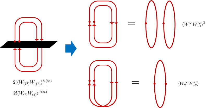
Figure 2: The graphical representation of the large $N$ rank-$2$ (anti)symmetric 2-point function. There is a unique way for each of contractions.

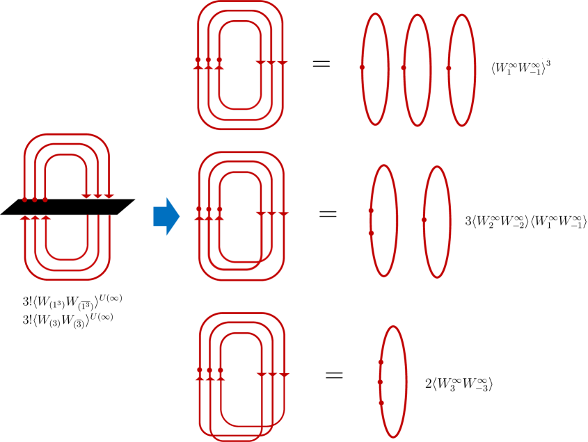
Figure 3: The graphical representation of the large $N$ rank-$3$ (anti)symmetric 2-point function. While for the top diagram there is a unique contraction, there are three for the middle and two for the bottom. These combinatorial factors determine the coefficients in (5.1.2).

We leave it future work to examine the fluctuation modes on the D3-brane dual giant in detail and compare them with those from the gravity side as studied in Faraggi:2011bb .

Using the conjectures (231) and (237), the generating function for the large $N$ limit of the 2-point functions of the Wilson line operators in the rank-$m$ (anti)symmetric representation is given by

$$\sum_{m=0}^{\infty}(s_{1}s_{2})^{m}\frac{\langle W_{(m)}W_{\overline{(m)}}\rangle^{U(\infty)}}{\mathcal{I}^{U(\infty)}} =\sum_{m=0}^{\infty}(s_{1}s_{2})^{m}\frac{\langle W_{(1^{m})}W_{\overline{(1^{m})}}\rangle^{U(\infty)}}{\mathcal{I}^{U(\infty)}}$$ (238)

$$=\exp\Biggl{[}\sum_{n=1}^{\infty}\frac{(s_{1}s_{2})^{n}}{n}\frac{1-q^{n}}{(1-q^{n/2}t^{2n})(1-q^{n/2}t^{-2n})}\Biggr{]}$$ (239)

$$=\frac{1-s_{1}s_{2}}{(s_{1}s_{2};q^{\frac{1}{2}}t^{2})_{\infty}(s_{1}s_{2};q^{\frac{1}{2}}t^{-2})_{\infty}}.$$ (240)

In the unflavored limit $t\to 1$, our result precisely reduces to the previous result in Drukker:2015spa .

5.2 Plane partition diamonds

The large $N$ limit of the unflavored Schur index of $\mathcal{N}=4$ $U(N)$ and $SU(N)$ SYM theory are identified with a generating function for the overpartition MR2034322 and the 3-colored partitions MR1634067 . Here we discuss the combinatorial interpretation of the Schur line defect correlator.

When the flavored fugacity $t$ is turned off, the 2-point function (236) can be written as

$$\langle W_{(m=\infty)}W_{\overline{(m=\infty)}}\rangle^{U(\infty)}(t=1;q)=\prod_{n=1}^{\infty}\frac{1-q^{n}}{(1-q^{\frac{n}{2}})^{4}}=\frac{(-q^{\frac{1}{2}};q^{\frac{1}{2}})_{\infty}}{(q^{\frac{1}{2}};q^{\frac{1}{2}})_{\infty}^{3}}.$$ (241)

This admits an expansion

$$\langle W_{(m=\infty)}W_{\overline{(m=\infty)}}\rangle^{U(\infty)}(t=1;q)=\sum_{n=0}d(n)q^{\frac{n}{2}}$$

$$=1+4q^{1/2}+13q+36q^{3/2}+90q^{2}+208q^{5/2}+455q^{3}+948q^{7/2}+1901q^{4}+\cdots.$$ (242)

The coefficient $d(n)$ is identified with the number of the Schmidt type partitions referred to as the plane partition diamonds of $n$ MR1868964 ; MR4370530 , that is the partitions of $n=a_{1}+a_{4}+a_{7}+\cdots$ whose parts $a_{i}$ lie on the graph which is made up of chains of rhombi in such a way that the set $(a_{3i-2},a_{3i-1},a_{3i},a_{3i+1})$ corresponds to the four vertices of the $i$-th rhombus with the conditions

$$a_{3i-2}\geq a_{3i-1}\geq a_{3i+1},\qquad a_{3i-2}\geq a_{3i}\geq a_{3i+1}.$$ (243)

For example, $d(1)$ counts the $4$ plane partition diamonds $\{a_{1}=1\}$, $\{a_{1}=1,a_{2}=1\}$, $\{a_{1}=1,a_{3}=1\}$ and $\{a_{1}=1,a_{2}=1,a_{3}=1\}$ and $d(2)$ counts the $13$ plane partition diamonds $\{a_{1}=1,a_{2}=1,a_{3}=1,a_{4}=1\}$, $\{a_{1}=1,a_{2}=1,a_{3}=1,a_{4}=1,a_{5}=1\}$, $\{a_{1}=1,a_{2}=1,a_{3}=1,a_{4}=1,a_{6}=1\}$, $\{a_{1}=1,a_{2}=1,a_{3}=1,a_{4}=1,a_{5}=1,a_{6}=1\}$, $\{a_{1}=2\}$, $\{a_{1}=2,a_{2}=2\}$, $\{a_{1}=2,a_{3}=2\}$, $\{a_{1}=2,a_{2}=2,a_{3}=2\}$, $\{a_{1}=2,a_{2}=1\}$, $\{a_{1}=2,a_{3}=1\}$, $\{a_{1}=2,a_{2}=1,a_{3}=1\}$ $\{a_{1}=2,a_{2}=2,a_{3}=1\}$ and $\{a_{1}=2,a_{2}=1,a_{3}=2\}$.

Let us study the degeneracy of the excitation modes of the D3-branes wrapping the $AdS_{2}\times S^{2}$ (or equivalently the D5-branes wrapping the $AdS_{2}\times S^{4}$). The growth of the number $d(n)$ of operators with large scaling dimension can be studied from the infinite product (241). Making use of the Meinardus Theorem MR62781 , we get the asymptotic growth

$$d(n)\sim\frac{7}{96n^{3/2}}\exp\left[\frac{7^{1/2}}{3^{1/2}}\pi n^{1/2}\right].$$ (244)

The exact numbers $d(n)$ and the values $d_{\textrm{asymp}}(n)$ obtained from the formula (244) are listed as follows:

$$\begin{array}[]{c|c|c}n&d(n)&d_{\textrm{asymp}}(n)\\ \hline\cr 10&6955&8982.37\\ 100&4.66051\times 10^{16}&5.05848\times 10^{16}\\ 1000&1.80784\times 10^{60}&1.85552\times 10^{60}\\ 5000&4.77308\times 10^{140}&4.82904\times 10^{140}\\ 10000&1.86714\times 10^{201}&1.88260\times 10^{201}\\ \end{array}$$ (251)

It should be compared with the asymptotic growth of the number of the states in the absence of the line operators, which is equal to the number of the overpartitions is given by Hatsuda:2022xdv

$$\overline{p}(n)\sim\frac{1}{8n}\left(1-\frac{1}{\pi n^{1/2}}\right)\exp\left[\pi n^{1/2}\right].$$ (252)

It would be interesting to elucidate the combinatorial aspects of the enumeration of the operators in the large $N$ limit and their asymptotic behaviors from the holographically dual supergravity.

Acknowledgements

The authors would like to thank Kimyeong Lee, Hai Lin and Masatoshi Noumi for useful discussions and comments. The work of Y.H. is supported in part by JSPS KAKENHI Grant No. 18K03657 and 22K03641. The work of T.O. is supported by the Startup Funding no. 4007012317 of the Southeast University.

Appendix A Definitions and notations

A.1 $q$-shifted factorial

We have used the following notation of $q$-shifted factorial:

$$(a;q)_{0} :=1,\qquad(a;q)_{n}:=\prod_{k=0}^{n-1}(1-aq^{k}),\qquad(q;q)_{n}:=\prod_{k=1}^{n}(1-q^{k}),\quad\quad n\geq 1,$$

$$(a;q)_{\infty} :=\prod_{k=0}^{\infty}(1-aq^{k}),\qquad(q;q)_{\infty}:=\prod_{k=1}^{\infty}(1-q^{k}),$$

$$(a^{\pm};q)_{\infty} :=(a;q)_{\infty}(a^{-1};q)_{\infty},$$ (253)

where $a$ and $q$ are complex variables.

A.2 Twisted Weierstrass functions

We define the twisted Weierstrass function by

$$P_{1}\left[\begin{matrix}\theta\\ \phi\\ \end{matrix}\right](z,\tau) =-{\sum_{n\in\mathbb{Z}}}^{\prime}\frac{x^{n+\lambda}}{1-\theta^{-1}q^{n+\lambda}},$$ (254)

and

$$P_{k}\left[\begin{matrix}\theta\\ \phi\\ \end{matrix}\right](z,\tau) =\frac{(-1)^{k}}{(k-1)!}\frac{1}{(2\pi i)^{k-1}}\frac{\partial^{k-1}}{\partial z^{k-1}}P_{1}\left[\begin{matrix}\theta\\ \phi\\ \end{matrix}\right](z,\tau)$$

$$=\frac{(-1)^{k}}{(k-1)!}{\sum_{n\in\mathbb{Z}}}^{\prime}\frac{(n+\lambda)^{k-1}x^{n+\lambda}}{1-\theta^{-1}q^{n+\lambda}},$$ (255)

where $\phi=e^{2\pi i\lambda}$.

Appendix B Multiple Kronecker theta series

The multiple Kronecker theta series (55) plays a role of elementary blocks of the Schur index and the Schur line defect correlators. They can be written in terms of the twisted Weierstrass functions. In this appendix, we show several examples.

B.1 $Q(l_{0},l_{1};n_{0},n_{1})$

In general the multiple Kronecker theta series (55) for $k=1$ is expandable from the equation (3.1.1). They show up in the closed-form expression of the Schur line defect 2-point functions.

The simplest example is $l_{0}=l_{1}=1$. We have

$$Q(1,1;0,n;u;\xi;q) =\sum_{p\in\mathbb{Z}}\frac{\xi^{-2p-n}}{(1-uq^{p})(1-uq^{p+n})}$$

$$=\frac{1}{1-q^{n}}\sum_{p\in\mathbb{Z}}\left(\frac{\xi^{-2p-n}}{(1-uq^{p})}-\frac{q^{n}\xi^{-2p-n}}{1-uq^{p+n}}\right)$$

$$=\Bigl{[}(n)_{q,\xi}+(-n)_{q,\xi}\Bigr{]}Q(1;0;u;\xi^{2};q)$$

$$=\Bigl{[}(n)_{q,\xi}+(-n)_{q,\xi}\Bigr{]}P_{1}\left[\begin{matrix}\xi^{2}\\ 1\\ \end{matrix}\right](\nu,\tau),$$ (256)

where we have assumed that $n$ is non-zero integer.

When $l_{0}=2$, $l_{1}=1$ and $n\neq 0$ we have

$$Q(2,1;0,n;u;\xi;q)$$

$$=-\frac{\xi^{-n}}{1-q^{n}}\sum_{p\in\mathbb{Z}}\frac{\xi^{-3p}}{(1-uq^{p})^{2}}+\frac{q^{n}\xi^{-n}}{(1-q^{n})^{2}}\sum_{p\in\mathbb{Z}}\frac{\xi^{-3p}}{1-uq^{p}}-\frac{q^{2n}\xi^{-n}}{(1-q^{n})^{2}}\sum_{p\in\mathbb{Z}}\frac{\xi^{-3p}}{1-uq^{p+n}}$$

$$=(n)_{q,\xi}Q(2;0;u;\xi^{\frac{3}{2}};q)+(1-q^{-n}\xi^{-3n})(-n)_{q,\xi}^{2}Q(1;0;u;\xi^{3};q),$$ (257)

$$Q(1,2;0,n;u;\xi;q)$$

$$=-\frac{\xi^{-2n}}{(1-q^{n})^{2}}\sum_{p\in\mathbb{Z}}\frac{\xi^{-3p}}{1-uq^{p}}+\frac{q^{n}\xi^{-2n}}{1-q^{n}}\sum_{p\in\mathbb{Z}}\frac{\xi^{-3p}}{(1-uq^{p+n})^{2}}+\frac{q^{n}\xi^{-2n}}{(1-q^{n})^{2}}\sum_{p\in\mathbb{Z}}\frac{\xi^{-3p}}{1-uq^{p+n}}$$

$$=(-n)_{q,\xi}Q(2;0;u;\xi^{\frac{3}{2}};q)+(1-q^{n}\xi^{3n})(n)_{q,\xi}^{2}Q(1;0;u;\xi^{3};q).$$ (258)

It follows that

$$Q(2,1;0,n;u;\xi;q)+Q(1;2;0,n;u;\xi;q)$$

$$=\frac{1}{u}\Bigl{[}(n)_{q,\xi}+(-n)_{q,\xi}\Bigr{]}P_{2}\left[\begin{matrix}q\xi^{3}\\ 1\\ \end{matrix}\right](\nu,\tau)-\Biggl{[}\frac{(n)_{q,\xi}^{2}}{(n)_{q\xi,1}}+\frac{(-n)_{q,\xi}^{2}}{(-n)_{q\xi,1}}\Biggr{]}P_{1}\left[\begin{matrix}\xi^{3}\\ 1\\ \end{matrix}\right](\nu,\tau).$$ (259)

For $l_{0}+l_{1}=3$ there are three types. When $n\neq 0$, we have

$$Q(3,1;0,n;u;\xi;q)$$

$$=(n)_{q,\xi}Q(3;0;u;\xi^{\frac{4}{3}};q)-q^{-n}\xi^{-3n}(-n)_{q,\xi}^{2}Q(2;0;u;\xi^{2};q)$$

$$+(1-q^{-n}\xi^{-4n})(-n)_{q,\xi}^{3}Q(1;0;u;\xi^{4};q)$$

$$=(n)_{q,\xi}Q(3,0;u;\xi^{\frac{4}{3}};q)-q^{n}\xi^{n}(n)_{q,\xi}^{2}Q(2;0;u;\xi^{2};q)-q^{2n}\xi^{2n}\frac{(n)_{q,\xi}^{3}}{(n)_{q\xi^{4},1}}Q(1;0;u;\xi^{4};q),$$ (260)

$$Q(2,2;0,n;u;\xi;q)$$

$$=\Bigl{[}(n)_{q,\xi}^{2}+(-n)_{q,\xi}^{2}\Bigr{]}Q(2;0;u;\xi^{2};q)-2q^{-n}\xi^{-n}(1-q^{-n}\xi^{-4n})(-n)_{q,\xi}^{3}Q(1;0;u;\xi^{4};q)$$

$$=\Bigl{[}(n)_{q,\xi}^{2}+(-n)_{q,\xi}^{2}\Bigr{]}Q(2;0;u;\xi^{2};q)-2\Bigl{[}q^{n}\xi^{n}(n)_{q,\xi}^{3}+q^{-n}\xi^{-n}(-n)_{q,\xi}^{3}\Bigr{]}Q(1;0;u;\xi^{4};q),$$ (261)

$$Q(1;3;0,n;u;\xi;q)$$

$$=(-n)_{q,\xi}Q(3;0;u;\xi^{\frac{4}{3}};q)-q^{n}\xi^{3n}(n)_{q,\xi}^{2}Q(2;0;u;\xi^{2};q)$$

$$+\Bigl{[}(n)_{q,\xi}^{2}+(-n)_{q,\xi}^{2}\Bigr{]}Q(2;0;u;\xi^{2};q)\left(1-q^{n}\xi^{4n}\right)(n)_{q,\xi}^{3}Q(1;0;u;\xi^{4};q)$$

$$=(-n)_{q,\xi}Q(3,0;u;\xi^{\frac{4}{3}};q)-q^{-n}\xi^{-n}(-n)_{q,\xi}^{2}Q(2;0;u;\xi^{2};q)-q^{-2n}\xi^{-2n}\frac{(-n)_{q,\xi}^{3}}{(-n)_{q\xi^{4},1}}Q(1;0;u;\xi^{4};q).$$ (262)

In terms of the twisted Weierstrass function they can be written as

$$Q(3,1;0,n;u;\xi;q)+Q(1,3;0,n;u;\xi;q)$$

$$=\frac{(n)_{q,\xi}+(-n)_{q,\xi}}{2u^{2}}\Bigl{(}P_{2}\left[\begin{matrix}q^{2}\xi^{3}\\ 1\\ \end{matrix}\right](\nu,\tau)+2P_{3}\left[\begin{matrix}q^{2}\xi^{3}\\ 1\\ \end{matrix}\right](\nu,\tau)\Bigr{)}$$

$$-\frac{q^{n}\xi^{n}(n)_{q,\xi}^{2}+q^{-n}\xi^{-n}(-n)_{q,\xi}^{2}}{u}P_{2}\left[\begin{matrix}q\xi^{4}\\ 1\\ \end{matrix}\right](\nu,\tau)-\Bigl{(}\frac{q^{2n}\xi^{2n}(n)_{q,\xi}^{3}}{(n)_{q\xi^{4},1}}+\frac{q^{-2n}\xi^{-2n}(-n)_{q,\xi}^{3}}{(-n)_{q\xi^{4},1}}\Bigr{)}P_{1}\left[\begin{matrix}\xi^{4}\\ 1\\ \end{matrix}\right](\nu,\tau),$$ (263)

$$Q(2,2;0,n;u;\xi;q)$$

$$=\frac{(n)_{q,\xi}^{2}+(-n)_{q,\xi}^{2}}{u}P_{2}\left[\begin{matrix}q\xi^{4}\\ 1\\ \end{matrix}\right](\nu,\tau)+2q^{n}\xi^{n}\frac{(n)_{q,\xi}^{3}}{(n)_{q\xi^{4},1}}P_{1}\left[\begin{matrix}\xi^{4}\\ 1\\ \end{matrix}\right](\nu,\tau).$$ (264)

B.2 $Q(l_{0},l_{1},l_{2};0,n_{0},n_{1},n_{2})$

We present several examples of the multiple Kronecker theta series (55) for $k=2$. They appear in the Schur line defect 3-point functions of the charged Wilson line operators. We assume that $n_{1}$ and $n_{2}$ are non-zero integers.

For $l_{0}=l_{1}=l_{2}=1$ the function (55) is given by

$$Q(1,1,1;0,n_{1},n_{2};u;\xi;q)$$

$$=\Bigl{[}(n_{1})_{q,\xi}(n_{2})_{q,\xi}+(-n_{1})_{q,\xi}(-n_{1}+n_{2})_{q,\xi}+(-n_{2})_{q,\xi}(-n_{2}+n_{1})_{q,\xi}\Bigr{]}Q(1;0;u;\xi^{3};q)$$

$$=\Bigl{[}(n_{1})_{q,\xi}(n_{2})_{q,\xi}+(-n_{1})_{q,\xi}(-n_{1}+n_{2})_{q,\xi}+(-n_{2})_{q,\xi}(-n_{2}+n_{1})_{q,\xi}\Bigr{]}P_{1}\left[\begin{matrix}\xi^{2}\\ 1\\ \end{matrix}\right](\nu,\tau).$$ (265)

When $l_{0}=2$, $l_{1}=l_{2}=1$ we have the expansion

$$Q(2,1,1;0,n_{1},n_{2};u;\xi;q)$$

$$=(n_{1})_{q,\xi}(n_{2})_{q,\xi}Q(2;0;u;\xi^{2};q)$$

$$-q^{-(n_{1}+n_{2})}\xi^{-3(n_{1}+n_{2})}(-q^{-n_{1}}-q^{-n_{2}}+2)(-n_{1})_{q,\xi}^{2}(-n_{2})_{q,\xi}^{2}Q(1;0;u;\xi^{4};q)$$

$$+(-n_{1})_{q,\xi}^{2}(-n_{1}+n_{2})_{q,\xi}Q(1;0;u;\xi^{4};q)$$

$$+(-n_{2})_{q,\xi}^{2}(-n_{2}+n_{1})_{q,\xi}Q(1;0;u;\xi^{4};q).$$ (266)

This leads to

$$Q(2,1,1;0,n_{1},n_{2};u;\xi;q)$$

$$=(n_{1})_{q,\xi}(n_{2})_{q,\xi}\frac{1}{u}P_{2}\left[\begin{matrix}q\xi^{4}\\ 1\\ \end{matrix}\right](\nu,\tau)+\Bigl{[}-q^{n_{1}+n_{2}}\xi^{n_{1}+n_{2}}(2-q^{-n_{1}}-q^{-n_{2}})(n_{1})_{q,\xi}^{2}(n_{2})_{q,\xi}^{2}$$

$$+(-n_{1})_{q,\xi}^{2}(-n_{1}+n_{2})_{q,\xi}+(-n_{2})_{q,\xi}^{2}(-n_{2}+n_{1})_{q,\xi}\Bigr{]}P_{1}\left[\begin{matrix}\xi^{4}\\ 1\\ \end{matrix}\right](\nu,\tau).$$ (267)

For $l_{0}=3$, $l_{1}=l_{2}=1$

$$Q(3,1,1;0,n_{1},n_{2};u;\xi;q)$$

$$=(n_{1})_{q,\xi}(n_{2})_{q,\xi}Q(3;0;u;\xi^{\frac{5}{3}};q)$$

$$-q^{-(n_{1}+n_{2})}\xi^{-3(n_{1}+n_{2})}(-q^{-n_{1}}-q^{-n_{2}}+2)(-n_{1})_{q,\xi}^{2}(-n_{2})_{q,\xi}^{2}Q(2;0;u;\xi^{\frac{5}{2}};q)$$

$$+q^{-(n_{1}+n_{2})}\xi^{-4(n_{1}+n_{2})}(-3q^{-n_{1}}-3q^{-n_{2}}+q^{-2n_{1}}+q^{-2n_{2}}+q^{-n_{1}-n_{2}}+3)(-n_{1})^{3}(-n_{2})^{3}Q(1;0;u;\xi^{5})$$

$$+(-n_{1})_{q,\xi}^{3}(-n_{1}+n_{2})_{q,\xi}Q(1;0;u;\xi^{5})$$

$$+(-n_{2})_{q,\xi}^{3}(-n_{2}+n_{1})_{q,\xi}Q(1;0;u;\xi^{5}).$$ (268)

For $l_{0}=4$, $l_{1}=l_{2}=1$

$$Q(4,1,1;0,n_{1},n_{2};u;\xi;q)$$

$$=(n_{1})_{q,\xi}(n_{2})_{q,\xi}Q(4;0;u;\xi^{\frac{3}{2}};q)$$

$$-q^{-(n_{1}+n_{2})}\xi^{-3(n_{1}+n_{2})}(-q^{-n_{1}}-q^{-n_{2}}+2)(-n_{1})_{q,\xi}^{2}(-n_{2})_{q,\xi}^{2}Q(3;0;u;\xi^{2};q)$$

$$+q^{-(n_{1}+n_{2})}\xi^{-4(n_{1}+n_{2})}(-3q^{-n_{1}}-3q^{-n_{2}}+q^{-2n_{1}}+q^{-2n_{2}}+q^{-n_{1}-n_{2}}+3)(-n_{1})^{3}(-n_{2})^{3}Q(2;0;u;\xi^{3})$$

$$-q^{-(n_{1}+n_{2})}\xi^{-5(n_{1}+n_{2})}(-6q^{-n_{1}}-6q^{-n_{2}}+4q^{-2n_{1}}+4q^{-2n_{2}}+4q^{-n_{1}-n_{2}}$$

$$-q^{-3n_{1}}-q^{-3n_{2}}-q^{-2n_{1}-n_{2}}-q^{-2n_{1}-n_{2}}+4)(-n_{1})_{q,\xi}^{4}(-n_{2})_{q,\xi}^{4}Q(1;0;u;\xi^{6};q)$$

$$+(-n_{1})_{q,\xi}^{4}(-n_{1}+n_{2})_{q,\xi}Q(1;0;u;\xi^{6})$$

$$+(-n_{2})_{q,\xi}^{4}(-n_{2}+n_{1})_{q,\xi}Q(1;0;u;\xi^{6}).$$ (269)

For $l_{0}=2$, $l_{1}=2$, $l_{2}=1$

$$Q(2,2,1;0,n_{1},n_{2};u;\xi;q)$$

$$=(n_{1})_{q,\xi}^{2}(n_{2})_{q,\xi}Q(2;0;u;\xi^{\frac{5}{2}};q)$$

$$-q^{-(2n_{1}+n_{2})}\xi^{-3(n_{1}+n_{2})-2n_{1}}(q^{-n_{1}}+2q^{-n_{2}}-3)(-n_{1})_{q,\xi}^{3}(-n_{2})_{q,\xi}^{2}Q(1;0;u;\xi^{3};q)$$

$$+(-n_{1})_{q,\xi}^{2}(-n_{1}+n_{2})_{q,\xi}Q(2;0;u;\xi^{\frac{5}{2}};q)$$

$$+q^{n_{2}-n_{1}}\xi^{n_{2}-2n_{1}}(-3q^{-n_{1}}+2q^{-2n_{1}}+1)(-n_{1})_{q,\xi}^{3}(-n_{1}+n_{2})_{q,\xi}^{2}Q(1;0;u;\xi^{5})$$

$$+(-n_{2})^{2}(-n_{2}+n_{1})^{2}Q(1;0;u;\xi^{5};q).$$ (270)

For $l_{0}=3$, $l_{1}=2$, $l_{2}=1$

$$Q(3,2,1;0,n_{1},n_{2};u;\xi;q)$$

$$=(n_{1})_{q,\xi}^{2}(n_{2})_{q,\xi}Q(3;0;u;\xi^{2};q)$$

$$-q^{-(2n_{1}+n_{2})}\xi^{-3(n_{1}+n_{2})-2n_{1}}(q^{-n_{1}}+2q^{-n_{2}}-3)(-n_{1})_{q,\xi}^{3}(-n_{2})_{q,\xi}^{2}Q(2;0;u;\xi^{3};q)$$

$$-q^{-(2n_{1}+n_{2})}\xi^{-4(n_{1}+n_{2})-2n_{1}}(-4q^{-n_{1}}-8q^{-n_{2}}+q^{-2n_{1}}+3q^{-2n_{2}}+2q^{-n_{1}-n_{2}}+6)$$

$$\times(-n_{1})_{q,\xi}^{4}(-n_{2})_{q,\xi}^{3}Q(1;0;u;\xi^{3};q)$$

$$+(-n_{1})_{q,\xi}^{3}(-n_{1}+n_{2})_{q,\xi}Q(2;0;u;\xi^{3};q)$$

$$+q^{n_{2}-n_{1}}\xi^{2n_{2}-3(n_{1}+n_{2})}(-4q^{-n_{1}}+3q^{-n_{2}}+1)(-n_{1})_{q,\xi}^{4}(-n_{1}+n_{2})_{q,\xi}^{2}Q(1;0;u;\xi^{6};q)$$

$$+(-n_{2})^{3}(-n_{2}+n_{1})^{2}Q(1;0;u;\xi^{6};q).$$ (271)

For $l_{0}=4$, $l_{1}=2$, $l_{2}=1$

$$Q(4,2,1;0,n_{1},n_{2};u;\xi;q)$$

$$=(n_{1})_{q,\xi}^{2}(n_{2})_{q,\xi}Q(4;0;u;\xi^{\frac{7}{4}};q)$$

$$-q^{-(2n_{1}+n_{2})}\xi^{-3(n_{1}+n_{2})-2n_{1}}(q^{-n_{1}}+2q^{-n_{2}}-3)(-n_{1})_{q,\xi}^{3}(-n_{2})_{q,\xi}^{2}Q(3;0;u;\xi^{\frac{7}{3}};q)$$

$$-q^{-(2n_{1}+n_{2})}\xi^{-4(n_{1}+n_{2})-2n_{1}}(-4q^{-n_{1}}-8q^{-n_{2}}+q^{-2n_{1}}+3q^{-2n_{2}}+2q^{-n_{1}-n_{2}}+6)$$

$$\times(-n_{1})_{q,\xi}^{4}(-n_{2})_{q,\xi}^{3}Q(2;0;u;\xi^{\frac{7}{2}};q)$$

$$-q^{-(2n_{1}+n_{2})}\xi^{-5(n_{1}+n_{2})-2n_{1}}(10q^{-n_{1}}+20q^{-n_{2}}-5q^{-2n_{1}}-15q^{-2n_{2}}-10q^{-n_{1}-n_{2}}$$

$$+q^{-3n_{1}}+4q^{-3n_{2}}+3q^{-n_{1}-2n_{2}}+2q^{-2n_{1}-n_{2}}-10)(-n_{1})_{q,\xi}^{5}(-n_{2})^{4}Q(1;0;u;\xi^{7};q)$$

$$+(-n_{1})_{q,\xi}^{4}(-n_{1}+n_{2})_{q,\xi}Q(2;0;u;\xi^{\frac{7}{2}};q)$$

$$+q^{n_{2}-n_{1}}\xi^{n_{2}-2n_{1}}(-5q^{-n_{1}}+4q^{-n_{2}}+1)(-n_{1})_{q,\xi}^{5}(-n_{1}+n_{2})_{q,\xi}^{2}Q(1;0;u;\xi^{7};q)$$

$$+(-n_{2})_{q,\xi}^{4}(-n_{2}+n_{1})_{q,\xi}^{2}Q(1;0;u;\xi^{7};q).$$ (272)

For $l_{0}=2$, $l_{1}=2$, $l_{2}=1$

$$Q(2,2,2;0,n_{1},n_{2};u;\xi;q)$$

$$=(n_{1})_{q,\xi}^{2}(n_{2})_{q,\xi}^{2}Q(2;0;u;\xi^{3};q)$$

$$+2q^{-(2n_{1}+2n_{2})}\xi^{-5(n_{1}+n_{2})}(q^{-n_{1}}+q^{-n_{2}}-2)(-n_{1})_{q,\xi}^{3}(-n_{2})_{q,\xi}^{3}Q(1;0;u;\xi^{2};q)$$

$$+(-n_{1})_{q,\xi}^{2}(-n_{2})_{q,\xi}^{2}Q(2;0;u;\xi^{3};q)$$

$$+2q^{n_{2}-n_{1}}\xi^{n_{2}-2n_{1}}(-2q^{-n_{1}}+q^{-n_{2}}+1)(-n_{1})_{q,\xi}^{3}(-n_{2})_{q,\xi}^{3}Q(1;0;u;\xi^{6};q)$$

$$+(-n_{1})_{q,\xi}^{2}(-n_{2})_{q,\xi}^{2}Q(2;0;u;\xi^{3};q)$$

$$+2q^{n_{1}-n_{2}}\xi^{n_{1}-2n_{2}}(-2q^{-n_{2}}+q^{-n_{1}}+1)(-n_{1})_{q,\xi}^{3}(-n_{2})_{q,\xi}^{3}Q(1;0;u;\xi^{6};q).$$ (273)

B.3 $Q(1,1,\cdots,1;\{n_{i}\})$

The multiple Kronecker theta series with $l_{0}=l_{1}=\cdots=l_{k}=1$ appears in the $U(k+1)$ $(k+1)$-point function of the charged Wilson line operators. It can be expanded in terms of the Kronecker theta function (57) by the relation (3.1.1).

For example,

$$Q(1,1;0,n;u;\xi;q) =\left[(n)_{q,\xi}+(-n)_{q,\xi}\right]Q(1;0;u;\xi^{2};q),$$ (274)

$$Q(1,1,1;0,n_{1},n_{2};u;\xi;q) =\Bigl{[}(n_{1})_{q,\xi}(n_{2})_{q,\xi}+(-n_{1})_{q,\xi}(-n_{1}+n_{2})_{q,\xi}$$

$$+(-n_{2})_{q,\xi}(-n_{2}+n_{1})_{q,\xi}\Bigr{]}Q(1;0;u;\xi^{3};q),$$ (275)

$$Q(1,1,1,1;0,n_{1},n_{2},n_{3};u;\xi;q) =\Bigl{[}(n_{1})_{q,\xi}(n_{2})_{q,\xi}(n_{3})_{q,\xi}$$

$$+(-n_{1})_{q,\xi}(-n_{1}+n_{2})_{q,\xi}(-n_{1}+n_{3})_{q,\xi}$$

$$+(-n_{2})_{q,\xi}(-n_{2}+n_{1})_{q,\xi}(-n_{2}+n_{3})_{q,\xi}$$

$$+(-n_{3})_{q,\xi}(-n_{3}+n_{1})_{q,\xi}(-n_{3}+n_{2})_{q,\xi}\Bigr{]}$$

$$\times Q(1;0;u;\xi^{4};q).$$ (276)

Appendix C Spectral zeta functions

C.1 $Z_{l}^{E}$

The 2-point functions of the Wilson line operators transforming in the antisymmetric representation for $\mathcal{N}=2^{*}$ $U(N)$ SYM theory are captured by the spectral zeta functions $Z_{l}^{E}(n)$, $l\leq N$. For $l=6$ we have

$$Z_{6}^{E} =(1+s_{1}^{6}s_{2}^{6})Q(6;0)+6(s_{1}s_{2}+s_{1}^{5}s_{2}^{5})\Bigl{[}Q(6;0)+Q(5,1;0,n)+Q(4,2;0,n)$$

$$+Q(3,3;0,n)+Q(2,4;0,n)+Q(1,5;0,n)\Bigr{]}+(s_{1}^{2}s_{2}^{2}+s_{1}^{4}s_{2}^{4})\Bigl{[}15Q(6;0)+24Q(5,1;0,n)$$

$$+33Q(4,2;0,n)+36Q(3,3;0,n)+22Q(2,4;0,n)+24Q(1,5;0,n)+6Q(3,2,1;0,n,2n)$$

$$+12Q(2,3,1;0,n,2n)+18Q(1,4,1;0,n,2n)+6Q(2,2,2;0,n,2n)+12Q(1,3,2;0,n,2n)$$

$$+6Q(1,2,3;0,n,2n)\Bigr{]}+s_{1}^{3}s_{2}^{3}\Bigl{[}20Q(6;0)+36Q(5,1;0,n)+54Q(4,2;0,n)$$

$$+62Q(3,3;0,n)+54Q(2,4;0,n)+36Q(1,5;0,n)+12Q(3,2,1;0,n,2n)$$

$$+30Q(2,3,1;0,n,2n)+36Q(1,4,1;0,n,2n)+12Q(2,2,2;0,n,2n)$$

$$+30Q(1,3,2;0,n,2n)+12Q(1,2,3;0,n,2n)+6Q(1,2,2,1;0,n,2n,3n)\Bigr{]}.$$ (277)

C.2 $Z_{l}^{H}$

For the 2-point functions of the Wilson line operators transforming in the rank-$k$ symmetric representation for $\mathcal{N}=2^{*}$ $U(N)$ SYM theory, we need the terms with $s_{1}^{k}s_{2}^{k}$ in the spectral zeta functions $Z_{l}^{H}(n)$, $l\leq N$.

For $l\geq 4$ and $k=0,1,2$ we have

$$Z_{4}^{H} =Q(4;0)+4s_{1}s_{2}\Bigl{[}Q(4;0)+Q(3,1;0,n)+Q(2,2;0,n)+Q(1,3;0,n)\Bigr{]}$$

$$+s_{1}^{2}s_{2}^{2}\Bigl{[}10Q(4;0)+16Q(3,1;0,n)+18Q(2,2;0,n)+16Q(1,3;0,n)$$

$$+4Q(3,1;0,2n)+4Q(2,2;0,2n)+4Q(3,1;0,2n)$$

$$+12(1,2,1;0,n,2n)+8(2,1,1;0,n,2n)+8(1,1,2;0,n,2n)\Bigr{]},$$ (278)

$$Z_{5}^{H} =Q(5;0)+5s_{1}s_{2}\Bigl{[}Q(5;0)+Q(4,1;0,n)+Q(3,2;0,n)$$

$$+Q(2,3;0,n)+Q(1,4;0,n)\Bigr{]}+s_{1}^{2}s_{2}^{2}\Bigl{[}15Q(5;0)+25Q(4,1;0,n)+30Q(3,2;0,n)$$

$$+30Q(2,3;0,n)+25Q(1,4;0,n)+5Q(4,1;0,n)+5Q(3,2;0,n)$$

$$+5Q(2,3;0,n)+5Q(1,4;0,n)+15Q(2,2,1;0,n,2n)+15Q(1,2,2;0,n,2n)$$

$$+10Q(2,1,2;0,n,2n)+20Q(1,3,1;0,n,2n)+10Q(3,1,1;0,n,2n)$$

$$+10Q(1,1,3;0,n,2n)\Bigr{]},$$ (279)

$$Z_{6}^{H} =Q(6;0)+6s_{1}s_{2}\Bigl{[}Q(6;0)+Q(5,1;0,n)+Q(4,2;0,n)+Q(3,3;0,n)$$

$$+Q(2,4;0,n)+Q(1,5;0,n)\Bigr{]}+s_{1}^{2}s_{2}^{2}\Bigl{[}21Q(6;0)+36Q(5,1;0,n)+45Q(4,2;0,n)$$

$$+48Q(3,3;0,n)+45Q(2,4;0,1)+36Q(1,5;0,n)+6Q(5,1;0,2n)$$

$$+6Q(4,2;0,2n)+6Q(3,3;0,2n)+6Q(2,4;0,2n)+6Q(1,5;0,2n)$$

$$+24Q(1,3,2;0,n,2n)+24Q(2,3,1;0,n,2n)+18Q(3,2,1;0,n,2n)$$

$$+18Q(1,2,3;0,n,2n)+12Q(3,1,2;0,n,2n)+12Q(2,1,3;0,n,2n)$$

$$+30Q(1,4,1;0,n,2n)+12Q(4,1,1;0,n,2n)+12Q(1,1,4;0,n,2n)$$

$$+18Q(2,2,2;0,n,2n)\Bigr{]}.$$ (280)

References

- (1) C. Romelsberger, “Counting chiral primaries in N = 1, d=4 superconformal field theories,” Nucl. Phys. B747 (2006) 329–353, arXiv:hep-th/0510060 [hep-th].
- (2) J. Kinney, J. M. Maldacena, S. Minwalla, and S. Raju, “An Index for 4 dimensional super conformal theories,” Commun. Math. Phys. 275 (2007) 209–254, arXiv:hep-th/0510251 [hep-th].
- (3) A. Gadde, L. Rastelli, S. S. Razamat, and W. Yan, “The 4d Superconformal Index from q-deformed 2d Yang-Mills,” Phys. Rev. Lett. 106 (2011) 241602, arXiv:1104.3850 [hep-th].
- (4) A. Gadde, L. Rastelli, S. S. Razamat, and W. Yan, “Gauge Theories and Macdonald Polynomials,” Commun. Math. Phys. 319 (2013) 147–193, arXiv:1110.3740 [hep-th].
- (5) C. Beem, M. Lemos, P. Liendo, W. Peelaers, L. Rastelli, and B. C. van Rees, “Infinite Chiral Symmetry in Four Dimensions,” Commun. Math. Phys. 336 no. 3, (2015) 1359–1433, arXiv:1312.5344 [hep-th].
- (6) A. Gadde, E. Pomoni, L. Rastelli, and S. S. Razamat, “S-duality and 2d Topological QFT,” JHEP 03 (2010) 032, arXiv:0910.2225 [hep-th].
- (7) Y. Pan and W. Peelaers, “Exact Schur index in closed form,” Phys. Rev. D 106 no. 4, (2022) 045017, arXiv:2112.09705 [hep-th].
- (8) C. Beem, S. S. Razamat, and P. Singh, “Schur indices of class S and quasimodular forms,” Phys. Rev. D 105 no. 8, (2022) 085009, arXiv:2112.10715 [hep-th].
- (9) T. Dimofte, D. Gaiotto, and S. Gukov, “3-Manifolds and 3d Indices,” Adv. Theor. Math. Phys. 17 no. 5, (2013) 975–1076, arXiv:1112.5179 [hep-th].
- (10) D. Gang, E. Koh, and K. Lee, “Line Operator Index on ,” JHEP 05 (2012) 007, arXiv:1201.5539 [hep-th].
- (11) N. Drukker, “The Schur index with Polyakov loops,” JHEP 12 (2015) 012, arXiv:1510.02480 [hep-th].
- (12) C. Cordova, D. Gaiotto, and S.-H. Shao, “Infrared Computations of Defect Schur Indices,” JHEP 11 (2016) 106, arXiv:1606.08429 [hep-th].
- (13) A. Neitzke and F. Yan, “Line defect Schur indices, Verlinde algebras and fixed points,” JHEP 11 (2017) 035, arXiv:1708.05323 [hep-th].
- (14) D. Gaiotto and J. Abajian, “Twisted M2 brane holography and sphere correlation functions,” arXiv:2004.13810 [hep-th].
- (15) Y. Pan and W. Peelaers, “Schur correlation functions on ,” JHEP 07 (2019) 013, arXiv:1903.03623 [hep-th].
- (16) M. Dedushenko and M. Fluder, “Chiral Algebra, Localization, Modularity, Surface defects, And All That,” J. Math. Phys. 61 no. 9, (2020) 092302, arXiv:1904.02704 [hep-th].
- (17) Y. Wang and Y. Pan, “Schur correlation functions from -deformed Yang-Mills theory,” Phys. Rev. D 103 no. 10, (2021) 106017, arXiv:2008.07126 [hep-th].
- (18) A. Buchel, J. G. Russo, and K. Zarembo, “Rigorous Test of Non-conformal Holography: Wilson Loops in N=2* Theory,” JHEP 03 (2013) 062, arXiv:1301.1597 [hep-th].
- (19) N. Bobev, H. Elvang, D. Z. Freedman, and S. S. Pufu, “Holography for on ,” JHEP 07 (2014) 001, arXiv:1311.1508 [hep-th].
- (20) X. Chen-Lin, J. Gordon, and K. Zarembo, “ super-Yang-Mills theory at strong coupling,” JHEP 11 (2014) 057, arXiv:1408.6040 [hep-th].
- (21) K. Zarembo, “Strong-Coupling Phases of Planar Super-Yang-Mills Theory,” Theor. Math. Phys. 181 no. 3, (2014) 1522–1530, arXiv:1410.6114 [hep-th].
- (22) X. Chen-Lin and K. Zarembo, “Higher Rank Wilson Loops in Super-Yang-Mills Theory,” JHEP 03 (2015) 147, arXiv:1502.01942 [hep-th].
- (23) X. Chen-Lin, A. Dekel, and K. Zarembo, “Holographic Wilson loops in symmetric representations in super-Yang-Mills theory,” JHEP 02 (2016) 109, arXiv:1512.06420 [hep-th].
- (24) X. Chen-Lin, D. Medina-Rincon, and K. Zarembo, “Quantum String Test of Nonconformal Holography,” JHEP 04 (2017) 095, arXiv:1702.07954 [hep-th].
- (25) J. T. Liu, L. A. Pando Zayas, and S. Zhou, “Comments on higher rank Wilson loops in ,” JHEP 01 (2018) 047, arXiv:1708.06288 [hep-th].
- (26) J. Bourdier, N. Drukker, and J. Felix, “The exact Schur index of SYM,” JHEP 11 (2015) 210, arXiv:1507.08659 [hep-th].
- (27) J. Bourdier, N. Drukker, and J. Felix, “The Schur index from free fermions,” JHEP 01 (2016) 167, arXiv:1510.07041 [hep-th].
- (28) Y. Hatsuda and T. Okazaki, “ = 2∗ Schur indices,” JHEP 01 (2023) 029, arXiv:2208.01426 [hep-th].
- (29) Kronecker, “On the theory of the elliptic functions.” Berl. Monatsber. 1881 (1881) 1165–1172.
- (30) A. Weil, Elliptic functions according to Eisenstein and Kronecker. Classics in Mathematics. Springer-Verlag, Berlin, 1999. Reprint of the 1976 original.
- (31) D. Zagier, “Periods of modular forms and Jacobi theta functions,” Invent. Math. 104 no. 3, (1991) 449–465. https://doi.org/10.1007/BF01245085.
- (32) A. Libgober, “Elliptic genera, real algebraic varieties and quasi-Jacobi forms,” in Topology of stratified spaces, vol. 58 of Math. Sci. Res. Inst. Publ., pp. 95–120. Cambridge Univ. Press, Cambridge, 2011.
- (33) C.-y. Dong, H.-s. Li, and G. Mason, “Modular invariance of trace functions in orbifold theory,” Commun. Math. Phys. 214 (2000) 1–56, arXiv:q-alg/9703016.
- (34) G. Mason, M. P. Tuite, and A. Zuevsky, “Torus n-point functions for R-graded vertex operator superalgebras and continuous fermion orbifolds,” Commun. Math. Phys. 283 (2008) 305–342, arXiv:0708.0640 [math.QA].
- (35) J. M. Maldacena, “Wilson loops in large N field theories,” Phys. Rev. Lett. 80 (1998) 4859–4862, arXiv:hep-th/9803002.
- (36) S.-J. Rey and J.-T. Yee, “Macroscopic strings as heavy quarks in large N gauge theory and anti-de Sitter supergravity,” Eur. Phys. J. C 22 (2001) 379–394, arXiv:hep-th/9803001.
- (37) N. Drukker and B. Fiol, “All-genus calculation of Wilson loops using D-branes,” JHEP 02 (2005) 010, arXiv:hep-th/0501109.
- (38) S. Yamaguchi, “Wilson loops of anti-symmetric representation and D5-branes,” JHEP 05 (2006) 037, arXiv:hep-th/0603208.
- (39) J. Gomis and F. Passerini, “Holographic Wilson Loops,” JHEP 08 (2006) 074, arXiv:hep-th/0604007.
- (40) D. Rodriguez-Gomez, “Computing Wilson lines with dielectric branes,” Nucl. Phys. B 752 (2006) 316–326, arXiv:hep-th/0604031.
- (41) S. A. Hartnoll and S. P. Kumar, “Multiply wound Polyakov loops at strong coupling,” Phys. Rev. D 74 (2006) 026001, arXiv:hep-th/0603190.
- (42) J. Gomis and F. Passerini, “Wilson Loops as D3-Branes,” JHEP 01 (2007) 097, arXiv:hep-th/0612022 [hep-th].
- (43) S. Yamaguchi, “Semi-classical open string corrections and symmetric Wilson loops,” JHEP 06 (2007) 073, arXiv:hep-th/0701052.
- (44) G. E. Andrews, P. Paule, and A. Riese, “MacMahon’s partition analysis. VIII. Plane partition diamonds,” vol. 27, pp. 231–242. 2001. https://doi.org/10.1006/aama.2001.0733. Special issue in honor of Dominique Foata’s 65th birthday (Philadelphia, PA, 2000).
- (45) G. E. Andrews and P. Paule, “MacMahon’s partition analysis XIII: Schmidt type partitions and modular forms,” J. Number Theory 234 (2022) 95–119. https://doi.org/10.1016/j.jnt.2021.09.008.
- (46) H. Rosengren, “Sums of triangular numbers from the Frobenius determinant,” Adv. Math. 208 no. 2, (2007) 935–961. https://doi.org/10.1016/j.aim.2006.04.006.
- (47) M. Ito and M. Noumi, “A determinant formula associated with the elliptic hypergeometric integrals of type ,” J. Math. Phys. 60 no. 7, (2019) 071705, 31. https://doi.org/10.1063/1.5094116.
- (48) I. G. Macdonald, Symmetric functions and Hall polynomials. Oxford Mathematical Monographs. The Clarendon Press, Oxford University Press, New York, second ed., 1995. With contributions by A. Zelevinsky, Oxford Science Publications.
- (49) Y. Ito, T. Okuda, and M. Taki, “Line operators on and quantization of the Hitchin moduli space,” JHEP 04 (2012) 010, arXiv:1111.4221 [hep-th]. [Erratum: JHEP 03, 085 (2016)].
- (50) N. Mekareeya and D. Rodriguez-Gomez, “5d gauge theories on orbifolds and 4d ‘t Hooft line indices,” JHEP 11 (2013) 157, arXiv:1309.1213 [hep-th].
- (51) T. D. Brennan, A. Dey, and G. W. Moore, “On ’t Hooft defects, monopole bubbling and supersymmetric quantum mechanics,” JHEP 09 (2018) 014, arXiv:1801.01986 [hep-th].
- (52) T. D. Brennan, A. Dey, and G. W. Moore, “’t Hooft defects and wall crossing in SQM,” JHEP 10 (2019) 173, arXiv:1810.07191 [hep-th].
- (53) H. Hayashi, T. Okuda, and Y. Yoshida, “ABCD of ’t Hooft operators,” JHEP 04 (2021) 241, arXiv:2012.12275 [hep-th].
- (54) K. Pilch and N. P. Warner, “N=2 supersymmetric RG flows and the IIB dilaton,” Nucl. Phys. B 594 (2001) 209–228, arXiv:hep-th/0004063.
- (55) A. Buchel, A. W. Peet, and J. Polchinski, “Gauge dual and noncommutative extension of an N=2 supergravity solution,” Phys. Rev. D 63 (2001) 044009, arXiv:hep-th/0008076.
- (56) D. Gaiotto and J. H. Lee, “The Giant Graviton Expansion,” arXiv:2109.02545 [hep-th].
- (57) J. G. Russo and K. Zarembo, “Evidence for Large-N Phase Transitions in N=2* Theory,” JHEP 04 (2013) 065, arXiv:1302.6968 [hep-th].
- (58) D. Gaiotto and T. Okazaki, “Dualities of Corner Configurations and Supersymmetric Indices,” JHEP 11 (2019) 056, arXiv:1902.05175 [hep-th].
- (59) T. Okazaki, “Mirror symmetry of 3D gauge theories and supersymmetric indices,” Phys. Rev. D100 no. 6, (2019) 066031, arXiv:1905.04608 [hep-th].
- (60) T. Okazaki, “Abelian dualities of boundary conditions,” JHEP 08 (2019) 170, arXiv:1905.07425 [hep-th].
- (61) M. Del Zotto, C. Vafa, and D. Xie, “Geometric engineering, mirror symmetry and ,” JHEP 11 (2015) 123, arXiv:1504.08348 [hep-th].
- (62) D. Xie, W. Yan, and S.-T. Yau, “Chiral algebra of the Argyres-Douglas theory from M5 branes,” Phys. Rev. D 103 no. 6, (2021) 065003, arXiv:1604.02155 [hep-th].
- (63) M. Buican and T. Nishinaka, “Conformal Manifolds in Four Dimensions and Chiral Algebras,” J. Phys. A 49 no. 46, (2016) 465401, arXiv:1603.00887 [hep-th].
- (64) C. Closset, S. Schafer-Nameki, and Y.-N. Wang, “Coulomb and Higgs Branches from Canonical Singularities: Part 0,” JHEP 02 (2021) 003, arXiv:2007.15600 [hep-th].
- (65) C. Closset, S. Giacomelli, S. Schafer-Nameki, and Y.-N. Wang, “5d and 4d SCFTs: Canonical Singularities, Trinions and S-Dualities,” JHEP 05 (2021) 274, arXiv:2012.12827 [hep-th].
- (66) K.-G. Schlesinger, “Some remarks on q-deformed multiple polylogarithms,” arXiv:math/0111022.
- (67) M. Kaneko, N. Kurokawa, and M. Wakayama, “A variation of Euler’s approach to values of the Riemann zeta function,” Kyushu J. Math. 57 no. 1, (2003) 175–192. https://doi.org/10.2206/kyushujm.57.175.
- (68) D. M. Bradley, “Multiple -zeta values,” J. Algebra 283 no. 2, (2005) 752–798. https://doi.org/10.1016/j.jalgebra.2004.09.017.
- (69) V. V. Zudilin, “Algebraic relations for multiple zeta values,” Uspekhi Mat. Nauk 58 no. 1(349), (2003) 3–32. https://doi.org/10.1070/RM2003v058n01ABEH000592.
- (70) J. Zhao, “Multiple -zeta functions and multiple -polylogarithms,” Ramanujan J. 14 no. 2, (2007) 189–221. https://doi.org/10.1007/s11139-007-9025-9.
- (71) Y. Ohno and J.-I. Okuda, “On the sum formula for the -analogue of non-strict multiple zeta values,” Proc. Amer. Math. Soc. 135 no. 10, (2007) 3029–3037. https://doi.org/10.1090/S0002-9939-07-08994-0.
- (72) Y. Ohno, J.-i. Okuda, and W. Zudilin, “Cyclic -MZSV sum,” J. Number Theory 132 no. 1, (2012) 144–155. https://doi.org/10.1016/j.jnt.2011.08.001.
- (73) Y. Takeyama, “The algebra of a -analogue of multiple harmonic series,” SIGMA Symmetry Integrability Geom. Methods Appl. 9 (2013) Paper 061, 15. https://doi.org/10.3842/SIGMA.2013.061.
- (74) A. Okounkov, “Hilbert schemes and multiple q-zeta values,” 1404.3873.
- (75) J. Castillo-Medina, K. Ebrahimi-Fard, and D. Manchon, “Unfolding the double shuffle structure of -multiple zeta values,” Bull. Aust. Math. Soc. 91 no. 3, (2015) 368–388. https://doi.org/10.1017/S0004972715000167.
- (76) J. Singer, “On Bradley’s -MZVs and a generalized Euler decomposition formula,” J. Algebra 454 (2016) 92–122. https://doi.org/10.1016/j.jalgebra.2016.01.006.
- (77) H. Bachmann and U. Kühn, “The algebra of generating functions for multiple divisor sums and applications to multiple zeta values,” Ramanujan J. 40 no. 3, (2016) 605–648. https://doi.org/10.1007/s11139-015-9707-7.
- (78) A. Milas, “Generalized multiple q-zeta values and characters of vertex algebras,” 2203.15642.
- (79) K. Ebrahimi-Fard, D. Manchon, and J. Singer, “The Hopf algebra of (-)multiple polylogarithms with non-positive arguments,” Int. Math. Res. Not. IMRN no. 16, (2017) 4882–4922. https://doi.org/10.1093/imrn/rnw128.
- (80) O. Schiffmann and E. Vasserot, “The elliptic Hall algebra and the -theory of the Hilbert scheme of ,” Duke Math. J. 162 no. 2, (2013) 279–366. https://doi.org/10.1215/00127094-1961849.
- (81) I. Cherednik, Double affine Hecke algebras, vol. 319 of London Mathematical Society Lecture Note Series. Cambridge University Press, Cambridge, 2005. https://doi.org/10.1017/CBO9780511546501.
- (82) M. Cirafici, “A note on discrete dynamical systems in theories of class ,” JHEP 05 (2021) 224, arXiv:2011.12887 [hep-th].
- (83) S. Gukov, P. Koroteev, S. Nawata, D. Pei, and I. Saberi, “Branes and DAHA Representations,” arXiv:2206.03565 [hep-th].
- (84) D. Gaiotto, G. W. Moore, and A. Neitzke, “Framed BPS States,” Adv. Theor. Math. Phys. 17 no. 2, (2013) 241–397, arXiv:1006.0146 [hep-th].
- (85) N. Drukker, J. Gomis, T. Okuda, and J. Teschner, “Gauge Theory Loop Operators and Liouville Theory,” JHEP 02 (2010) 057, arXiv:0909.1105 [hep-th].
- (86) L. F. Alday, D. Gaiotto, S. Gukov, Y. Tachikawa, and H. Verlinde, “Loop and surface operators in N=2 gauge theory and Liouville modular geometry,” JHEP 01 (2010) 113, arXiv:0909.0945 [hep-th].
- (87) J. Gomis, T. Okuda, and V. Pestun, “Exact Results for ’t Hooft Loops in Gauge Theories on ,” JHEP 05 (2012) 141, arXiv:1105.2568 [hep-th].
- (88) Y. Hatsuda and T. Okazaki, “Fermi-gas correlators of ADHM theory and triality symmetry,” SciPost Phys. 12 (2022) 005, arXiv:2107.01924 [hep-th].
- (89) G. Frobenius, “Über die elliptischen Funktionen zweiter,” Art, J. Reine Angew. Math 93 (1882) 53–68.
- (90) J. D. Fay, Theta functions on Riemann surfaces. Lecture Notes in Mathematics, Vol. 352. Springer-Verlag, Berlin-New York, 1973.
- (91) Y. Hatsuda, M. Honda, S. Moriyama, and K. Okuyama, “ABJM Wilson Loops in Arbitrary Representations,” JHEP 10 (2013) 168, arXiv:1306.4297 [hep-th].
- (92) J. M. Maldacena, “The Large N limit of superconformal field theories and supergravity,” Adv.Theor.Math.Phys. 2 (1998) 231–252, arXiv:hep-th/9711200 [hep-th].
- (93) N. Drukker, D. J. Gross, and H. Ooguri, “Wilson loops and minimal surfaces,” Phys. Rev. D 60 (1999) 125006, arXiv:hep-th/9904191.
- (94) J. K. Erickson, G. W. Semenoff, and K. Zarembo, “Wilson loops in N=4 supersymmetric Yang-Mills theory,” Nucl. Phys. B 582 (2000) 155–175, arXiv:hep-th/0003055.
- (95) N. Drukker and D. J. Gross, “An Exact prediction of N=4 SUSYM theory for string theory,” J. Math. Phys. 42 (2001) 2896–2914, arXiv:hep-th/0010274.
- (96) S. Yamaguchi, “Bubbling geometries for half BPS Wilson lines,” Int. J. Mod. Phys. A 22 (2007) 1353–1374, arXiv:hep-th/0601089.
- (97) A. Faraggi and L. A. Pando Zayas, “The Spectrum of Excitations of Holographic Wilson Loops,” JHEP 05 (2011) 018, arXiv:1101.5145 [hep-th].
- (98) O. Lunin, “On gravitational description of Wilson lines,” JHEP 06 (2006) 026, arXiv:hep-th/0604133.
- (99) E. D’Hoker, J. Estes, and M. Gutperle, “Gravity duals of half-BPS Wilson loops,” JHEP 06 (2007) 063, arXiv:0705.1004 [hep-th].
- (100) T. Okuda and D. Trancanelli, “Spectral curves, emergent geometry, and bubbling solutions for Wilson loops,” JHEP 09 (2008) 050, arXiv:0806.4191 [hep-th].
- (101) J. Gomis, S. Matsuura, T. Okuda, and D. Trancanelli, “Wilson loop correlators at strong coupling: From matrices to bubbling geometries,” JHEP 08 (2008) 068, arXiv:0807.3330 [hep-th].
- (102) A. Faraggi, W. Mueck, and L. A. Pando Zayas, “One-loop Effective Action of the Holographic Antisymmetric Wilson Loop,” Phys. Rev. D 85 (2012) 106015, arXiv:1112.5028 [hep-th].
- (103) K. Okuyama and G. W. Semenoff, “Wilson loops in N=4 SYM and fermion droplets,” JHEP 06 (2006) 057, arXiv:hep-th/0604209.
- (104) S. Corteel and J. Lovejoy, “Overpartitions,” Trans. Amer. Math. Soc. 356 no. 4, (2004) 1623–1635. https://doi.org/10.1090/S0002-9947-03-03328-2.
- (105) G. E. Andrews, The theory of partitions. Cambridge Mathematical Library. Cambridge University Press, Cambridge, 1998. Reprint of the 1976 original.
- (106) G. Meinardus, “Asymptotische Aussagen über Partitionen,” Math. Z. 59 (1954) 388–398. https://doi.org/10.1007/BF01180268.