Quantum Approximate Optimization via Learning-based Adaptive Optimization

Abstract

Combinatorial optimization problems are ubiquitous and computationally hard to solve in general. Quantum computing is envisioned as a powerful tool offering potential computational advantages for solving some of these problems. Quantum approximate optimization algorithm (QAOA), one of the most representative quantum-classical hybrid algorithms, is designed to solve certain combinatorial optimization problems by transforming a discrete optimization problem into a classical optimization problem over a continuous circuit parameter domain. QAOA objective landscape over the parameter variables is notorious for pervasive local minima and barren plateaus, and its viability in training significantly relies on the efficacy of the classical optimization algorithm. To enhance the performance of QAOA, we design double adaptive-region Bayesian optimization (DARBO), an adaptive classical optimizer for QAOA. Our numerical results demonstrate that the algorithm greatly outperforms conventional gradient-based and gradient-free optimizers in terms of speed, accuracy, and stability. We also address the issues of measurement efficiency and the suppression of quantum noise by conducting the full optimization loop on a superconducting quantum processor as a proof of concept. This work helps to unlock the full power of QAOA and paves the way toward achieving quantum advantage in practical classical tasks.

I Introduction

Combinatorial optimization, which involves identifying an optimal solution from a finite set of candidates, has a wide range of applications across various fields, such as logistics, finance, physics, and machine learning. However, the problem in many typical scenarios is NP-hard since the set of feasible solutions is discrete and expands exponentially with the growing problem size without any structure that seems to admit polynomial-time algorithms. As a representative NP-hard problem, MAX-CUT aims to find a bi-partition of the input graph’s vertices, such that the number of edges (or total edge weights) between the two subsets reaches the maximum. Classical approaches such as greedy algorithms and AI methods by graph neural networks, despite remarkable attempts and progresses [1, 2, 3], are generally inefficient to address combinatorial optimization problems such as MAX-CUT due to their NP-hard nature. In the recent two decades, quantum computing approaches have emerged as a new toolbox for tackling these difficult but crucial problems, including quantum annealing [4, 5, 6, 7, 8] and quantum approximate optimization algorithm (QAOA) [9, 10, 11, 12, 13], from both theoretical and experimental perspectives. In this article, we focus on the latter paradigm, which is fully compatible with the universal gate-based quantum circuit model and is considered to be one of the most promising algorithms in the noisy intermediate-scale quantum (NISQ) era for potential quantum advantages.

In the QAOA paradigm, the exponential solution space is encoded in the Hilbert space of the output wavefunction of a parameterized quantum circuit. By this, the classical optimization problems in the discrete domain are relaxed to a continuous domain composed of circuit variational parameters via QAOA as a proxy. However, the classical optimization over the continuous circuit parameter domain is still challenging (the worst case is NP-hard [14]) since the energy landscape of the QAOA ansatz is filled with local minima and a large amount of independent optimization processes is required to identify a near-optimal solution [15, 10]. In addition, barren plateaus can also emerge in the QAOA landscape with increasing qubit number or circuit depth [16, 17, 18, 19]. To overcome these optimization difficulties, various learning-based [20, 21, 22, 23, 24, 25, 26, 27, 28] or heuristic-based approaches [10, 29, 30, 31, 32, 33] have previously been explored. These methods either rely on optimization data previously obtained or require a huge number of circuit evaluation budgets in total by progressively searching solutions of QAOA with different depths. A universally efficient and effective optimization approach suitable for real quantum processors without prior knowledge remains elusive.

In this work, we design a novel gradient-free classical optimizer dubbed Double Adaptive-Region Bayesian Optimization (DARBO), which exploits and explores the QAOA landscape with a Gaussian process (GP) surrogate model and iteratively suggests the most possible optimized parameter set restricted by two auto-adaptive regions, i.e., an adaptive trust region and an adaptive search region. The performance of DARBO for QAOA and ultimately for combinatorial optimization problems in terms of speed, stability, and accuracy is superior to existing methods. Furthermore, DARBO is robust against measurement shot noise and quantum noise. We demonstrated its effectiveness in extensive numerical simulations as well as a proof of concept demonstration of the quantum-classical optimization pipeline, where QAOA is implemented and evaluated on a real superconducting quantum processor using five qubits with integrated quantum error mitigation (QEM) techniques.

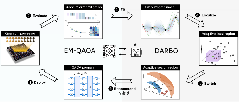
Figure 1: The proof-of-concept workflow for error mitigated QAOA on the superconducting quantum processor with DARBO. We compile and deploy the 5-qubit QAOA program for given objective functions on a 20-qubit real superconducting quantum processor and evaluate the objective value with quantum error mitigation methods. DARBO treats the EM-QAOA as a black-box, and optimizes the circuit parameters by fitting the surrogate model with constraints. The constraints are provided by the two adaptive regions, which are responsible for surrogate model building and acquisition function sampling, respectively.

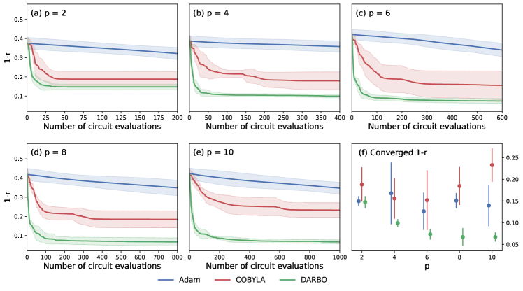
Figure 2: QAOA optimization for MAX-CUT problem on $n=16$ w3R graphs (exact simulations). (a)-(e) The optimization trajectories from different optimizers (Adam, COBYLA, and DARBO) are plotted versus the number of circuit evaluations. Results on different circuit depths from $p=2$ to $p=10$ are reported, respectively. (f) The final converged approximation gap $1-r$ after sufficient numbers of optimization iterations. For each circuit evaluation, we query the exact expectation of the objective function via numerical simulation. Each line is averaged over five w3R graph instances, where the shaded range shows the standard deviation of the results across different graph instances. For each graph instance, the best optimization result among the 20 independent optimization trials is reported. The error bar in (f) shows the standard deviation across different graph instances.

II QAOA framework with DARBO

MAX-CUT problem and a large family of combinatorial optimization problems can be embedded into a more general formalism as quadratic unconstrained binary optimization (QUBO) [34], where the objective function $C(\bf{z})$ to optimize is in the form as follows in terms of binary-valued variables $\bf{z}$:

$${C(\mathbf{z})=\sum_{ij}w_{ij}z_{i}z_{j},}$$ (1)

where $w_{ij}$ can be regarded as the edge weights defined on a given graph.

The QAOA framework is designed as a quantum-enhanced method to solve these QUBO problems. The quantum circuit ansatz for QAOA consists of the repetitive applications of two parameterized unitary operators. We denote the number of repetitions as $p$, and the number of qubits (binary freedoms in QUBO) as $n$. The quantum program ansatz is constructed as

$$|\psi(\mathbf{\gamma},\mathbf{\beta})\rangle=U(\mathbf{\gamma},\mathbf{\beta})|0^{n}\rangle=$$

$$\prod_{k=1}^{p}\left(e^{-i\beta_{k}\sum_{i}^{n}X_{i}}e^{-i\gamma_{k}\sum_{ij}w_{ij}Z_{i}Z_{j}}\right)\prod_{i}^{n}H_{i}|0^{n}\rangle,$$ (2)

where $X$ and $Z$ are Pauli matrice on each site and $H$ are Hadamard gate. The trainable parameters $\bf{\gamma}$ and $\bf{\beta}$ both consist $p$ real-valued components, and the outer classical training loop adjusts these parameters so that the objective $C(\gamma,\beta)=\langle\psi(\gamma,\beta)|\sum_{ij}w_{ij}Z_{i}Z_{j}|\psi(\gamma,\beta)\rangle$ is minimized. Therefore, by utilizing the QAOA framework, the optimization over discrete binary $\bf{z}$ variables is reduced to the optimization over continuous variables of $\beta$ and $\gamma$.

However, the continuous optimization problem still faces lots of pressing challenges. In the QAOA framework, gradient descent optimizers commonly utilized in the deep learning community do not work well. The common ansatze consisting of a large number of parameters can enjoy the benefits of over-parameterization and their global minima are easier to locate [35, 36]. However, QAOA ansatz has a small number of parameters and thus a large number of local minima, which often destroys the effort of conventional optimizers to identify the global minimum. Besides, barren plateaus that render the gradient variance vanishing exponentially can occur similarly as the generic cases in variational quantum algorithms. More importantly, gradient evaluations on real quantum chips are too noisy and costly to use for a classical optimizer.

Bayesian optimization (BO) is a class of black-box and gradient-free classical optimization approaches that can effectively optimize expensive black-box functions and tolerate stochastic noise in function evaluations. The method typically creates a surrogate for the unknown objective, and quantifies and manages the uncertainty using a Bayesian learning framework [37, 38]. Although conventional BO has become a highly competitive technique for solving optimizing problems with a small number of parameters, it usually does not scale well to problems with high dimensions [37, 38, 39, 40]. Aside from the plentiful local minima in the exponentially large search space, another challenge with BO is that the surrogate function fitting with very few samples can hardly be globally accurate.

To overcome the above issues and enable efficient QAOA executions on real quantum chips, we propose DARBO as a powerful classical optimizer for QAOA. The schematic quantum-classical hybrid workflow for DARBO-enabled QAOA is shown in Fig. 1. The advantages of DARBO are both from its Bayesian optimization nature and the two adaptive regions utilized in the algorithm. The idea of including an adaptive trust region is directly borrowed from TuRBO [38] and is inspired by a class of trust region methods from stochastic optimization [41]. These methods utilize a simple surrogate model inside a trust region centered on the current best solution. For instance, COBYLA [42] method used as a baseline in this work models the objective function locally with a linear model. As a deterministic approach, COBYLA is not good at handling noisy observations. By integrating with GP surrogate models within an adaptive trust region, DARBO inherits the robustness to noise and rigorous reasoning about uncertainties that global BO enjoys as well as the benefits that local surrogate model enables. In addition, the introduction of an adaptive search region makes DARBO more robust to different initial guesses by moving queries in some iterations to a more restricted region. The search efficiency increases when the search space is reduced by the adaptive search region, giving DARBO a higher chance of finding the global minimum rather than local minima.

In this study, the end-to-end performance of QAOA with DARBO is evaluated and benchmarked on the basis of analytical exact simulation, numerical simulation with measurement shot noise, and quantum hardware experiments (with both measurement shot noise and quantum noise). Overall, DARBO outperforms other common optimizers by a large margin in terms of 1) efficiency: the number of circuit evaluations to reach a given accuracy is the least, 2) stability: the fluctuation of the converged objective value across different initializations and graph instances is the least, 3) accuracy: the final converged approximation ratio is the best, and 4) noise robustness: the performance advantage is getting larger when noise presents, which is unavoidably the case on quantum processors.

III Results

We use approximation ratio $r$ as a metric to measure the end-to-end performance of QAOA. In MAX-CUT problem, $r$ is defined as the ratio of obtained cut value derived from the objective expectation over the exact max cut value ($r=1$ indicates a perfect solution for the problem), and $1-r$ is the (relative) approximation gap. Throughout this work, we investigate the MAX-CUT problem on the w3R graph which is a family of regular weighted graphs whose vertices all have degrees of three.

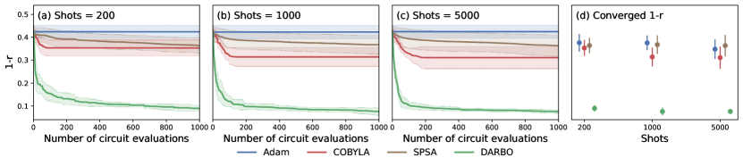
Figure 3: QAOA optimization for MAX-CUT problem on $n=16$ w3R graph with $p=10$ (simulation with measurement shot noise). (a)-(c) The optimization trajectories from different optimizers (Adam, COBYLA, SPSA, and DARBO) in terms of the number of circuit evaluations. Results on different shots number from $\text{shots}=200$ to $\text{shots}=5000$ are reported, respectively. (f) The final converged approximation ratio $1-r$ after sufficient numbers of optimization iterations. For each circuit evaluation, we collect the number of shot measurements to further reconstruct the loss expectation value. Each line is averaged over five w3R graph instances where the shaded range shows the standard deviation of the results across different graph instances. For each graph instance, the best optimization result from 20 independent optimization trials is kept. The error bar in (d) shows the standard deviation across different graph instances.

Analytically exact simulation

We firstly report the results on optimization trajectories and final converged objective values for analytically exact quantum simulation, which computes the objective function by directly evaluating the expectations from the wavefunction. Fig. 2 shows the results for a collection of different optimizers, including Adam [43], COBYLA [42], and DARBO. (For benchmark with more choices of common optimizers, see the Supplemental Material.) The results are collected from five different $n=16$ w3R graph instances, and for each graph and each optimization method, the best record over $20$ independent optimization trials is reported. The results show the superior efficiency of DARBO over other common optimizers. For all different $p$ values, the approximation gaps $1-r$ of Adam and COBYLA are $1.02\sim 2.08$ times and $1.28\sim 3.47$ times larger than those of DARBO, respectively. In addition to the efficiency and accuracy, the DARBO performance is also more stable in terms of different problem graph instances. We also report the results for fidelity in the Supplemental Material, which essentially gives the probability of obtaining the exact solution state from measuring the QAOA circuit.

It is worth noting that stability is of great importance for optimizing over the QAOA parameter landscape, as the great number of local minima requires generically exponential independent optimization trials to reach a global minimum [10]. As a result, with the increasing depth $p$ of QAOA, the optimization problem becomes harder, and we see that Adam and COBYLA do not even exhibit a monotonic growth of the accuracy as $p$ increases, despite the fact that the cut size given by the optimal $|\psi(\gamma,\beta)\rangle$ (over the choice of $2p$ parameters $(\gamma,\beta)$) is clearly non-decreasing with $p$. The reason of the performance drop is due to a lack of training stability and the sensitivity on initial parameter choices for conventional local optimization methods. DARBO, on the contrary, does give better results with large depth $p$. In other words, one important optimization advantage brought by DARBO is its capability of finding the near optimal parameters with a small number of independent optimization trials, which are not enough to locate the global optimal parameters for conventional optimizers. Some advanced optimization methods such as FOURIER heuristics reported in [10] can be good at locating global minimum but depend on progressive optimization on lower-depth QAOA, leading to a much larger total amount of required circuit evaluations.

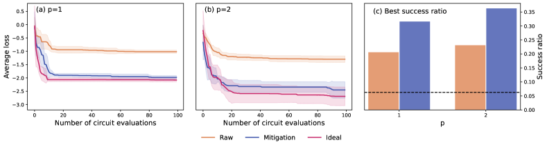
Figure 4: Quantum optimization of a five-variable QUBO problem on real quantum hardware with $\text{shots}=10000$. (a)-(b) show results from $p=1$ and $p=2$ QAOA, respectively. The line is the average optimization trajectory of five independent optimization trials, while the shaded area represents the standard deviation across five independent optimization trials. Averaged loss refers to the expectation value of the problem QUBO Hamiltonian. Raw: at each step, we obtain the loss expectation directly from measurement results on the real quantum processor. Mitigation: at each step, we obtain the loss expectation from measurement results integrated with QEM techniques. Ideal: at each step, we obtain the loss from numerical simulation. (c) The success ratio when we run inference on the trained QAOA program, i.e., the probability that we can obtain a correct bitstring answer for the problem on real quantum hardware. The dashed line is the random guess baseline with a probability of $1/16$. We report the best success ratio of the five optimization trials.

Numerical simulation with finite measurement shots

With the introduction of noise, DARBO shows more advantageous results compared to other optimizers, including Adam [43], COBYLA [42] and SPSA [44]. In Fig. 3, we show the optimization results of QAOA on five different $n=16$ w3R graph instances with $p=10$ with different measurement shots at each iteration, and for each graph and each optimization method, the best record over $20$ independent optimization processes is reported. For results on QAOA of different $p$, see the Supplemental Material. Since QAOA for MAX-CUT has a commutable objective function, the budgets of the measurement shots are all taken on the computational basis. It is natural that with more measurement shots, better accuracy could be achieved for the objective evaluation. Taking $m$ as the given number of measurement shots, we evaluate the final QUBO objective by reconstructing from measurement bitstrings represented by binary valued $z_{ij}=\pm 1$ where $i\leq m$ runs over different shots and $j\leq n$ runs over different qubits. The objective value $C$ is estimated as

$$C=\frac{1}{m}\sum_{i=1}^{m}\sum_{j=1}^{n}\sum_{k=1}^{n}w_{jk}z_{ij}z_{ik}.$$ (3)

This value is a random variable with a Gaussian distribution whose mean value is determined by the analytical expectation value of the objective function, and the standard deviation is controlled by the number of total shots $m$ with $\frac{1}{\sqrt{m}}$ scaling.

For DARBO, we can reach a satisfying optimized objective value with a small number of circuit evaluations, e.g., $200$ measurement shots at each round are more than enough. The optimization efficiency gets further improved with an increased number of measurement shots. In Fig. 3, the approximation gaps $1-r$ of Adam, COBYLA, and SPSA are $4.20\sim 4.59$, $3.95\sim 4.10$, and $4.07\sim 4.79$ times larger than those of DARBO, respectively. Besides, the solution quality from DARBO across different problem instances is impressively stable. The efficiency, accuracy, and stability of DARBO are all much better than those of other optimizers evaluated in our experiments. In addition, the performance gap between DARBO and other optimizers is getting larger compared to the infinite measurement shots (analytical exact) case, which reflects the noise robustness and adaptiveness of our proposed optimizer.

As a gradient-free optimization approach, Bayesian optimization has the advantages of robustness to noise and rigorous reasoning about uncertainty. Naïve BO methods have already been utilized to optimize variational quantum algorithms [45, 46, 47, 48], but they often suffer from the low efficiency. Benefiting from the adaptive trust region and local Gaussian process (GP) surrogate model, DARBO has better potential to optimize noisy problems [38]. Instead of directly using the currently best-observed solution $x^{*}$, we use the observation with the smallest posterior mean under the surrogate model, and therefore the noise affecting $x^{*}$ has limited effects on the optimization. DARBO is specifically suitable for optimization with shot noises induced by statistical uncertainty of finite measurement shots, since its GP surrogate model assumes that the observations are Gaussian-distributed random variables [49] which is consistent with the case for measurement results with finite shot noises.

Experiments on superconducting quantum hardware

Finally, we run QAOA equipped with DARBO on real quantum hardware to demonstrate its performance. Quantum error, in addition to shot noise, has a huge impact on optimization performance on real quantum hardware. It has been studied that quantum noises would in general flatten the objective function landscape and induce barren plateaus in variational quantum algorithms [50]. Here we investigate the effect of quantum noise on the performance of DARBO for QAOA, and at the same time analyze how the common error mitigation strategies [51, 52, 53, 54] can help in the DARBO process and achieve better end-to-end results.

The target problem is to optimize a five-variable QUBO (see the Supplemental Material for the problem definition in detail). The experimental results are shown in Fig. 4. We carry out the optimization on 1) raw objective value directly evaluated from measurement results on real hardware, 2) mitigation objective value evaluated from measurement results on real hardware with integrated quantum error mitigation techniques including layout benchmarking, readout error mitigation, and zero-noise extrapolation, see Method for more details, and 3) numerical exact value without quantum noise as a comparison. The optimization results are shown in terms of objective optimization history and success ratio from sampling the final QAOA circuit. Although the expectation value is conveniently taken as the objective value for the optimization process, the success ratio is another important representative metric to straightforwardly evaluate the final performance of QAOA for the QUBO objective since the true objective value can be directly reconstructed by the bitstring measured.

We noticed that DARBO conducted even on raw measurements can improve the cut estimation from the initial value, although it is not good enough compared to the ideal one due to the large influence of quantum noise. The optimization results combined with QEM are much better than the raw evaluations, both in terms of objective evaluation and success ratio from sampling the final QAOA circuit. Moreover, the performance gap between optimization on the mitigation value from experiments and that on the ideal value from numerics becomes larger for larger $p$, which is consistent with the fact that deeper circuits bring larger quantum noise. Still, we show that a deeper QAOA with $p=2$ gives a better approximation of the QUBO objective than a shallow QAOA with $p=1$, achieving a better trade-off between expressiveness and the accumulated noise.

The raw data collected directly from real quantum hardware contain both quantum noises and measure shot noises, which are essentially the bias and variances from the perspective of machine learning. In this EM-QAOA + DARBO framework, QEM helps to reduce the effects of bias on the hardware (gate noises, readout noises, decoherence noises and so on) by mitigating these errors, and DARBO avoids the negative influence of variances from repetitive measurements (shot noises). Therefore, these two key components together make the proposed framework a powerful optimization protocol for combinatorial optimization problems.

IV Discussion

With a better exploration of the QAOA landscape, the optimization routine based on Bayesian optimization shows weak initial parameter dependence and a better probability of escaping the local minimum. Although, in this work, the dimension of the parameter spaces is still relatively low, an interesting future direction is to generalize similar BO methods from the QAOA setup to other variational quantum algorithms, which has a larger number of parameters. Recently, several advanced BO variants have been proposed to increase the optimization efficiency and robustness in high-dimensional problems [55, 40, 56] and in problems with noisy observations [39, 57, 58, 59]. These approaches show superior optimization performances in challenging benchmarks with large parameter sizes and the presence of noises. For instance, an advanced BO approach could efficiently optimize a higher dimensional problem ($D=385$) [55], and accurately find the best experimental settings for the real-world problems in chemistry [60], material sciences [61], and biology [62]. These cases are potentially relevant for optimization in variational quantum eigensolver, quantum machine learning, and quantum architecture search scenarios.

We also note that the double-adaptive region idea in BO is a general framework. The detail settings in the DARBO approach could be designed differently for different optimization problems. As a future direction, DARBO algorithm could be extended to include more than two adaptive search regions, and the ranges of these regions themselves could also be adapted during the optimizations.

To successfully scale the QAOA program on real quantum hardware with meaningful accuracy, more pruning and compiling techniques for QAOA deployment, as well as more error mitigation techniques, can be utilized in future works. For example, by differentiable quantum architecture search-based compiling [63], we can greatly reduce the number of two-qubit quantum gates required with even better approximation performance. There is also QAOA tailored error mitigation algorithm [64] that trades qubit space for accuracy.

In summary, we proposed an optimizer - DARBO suitable for exploring the variational quantum algorithm landscapes and applied it to the QAOA framework for solving combinatorial problems. The end-to-end performance for combinatorial problems is greatly improved in both numerical simulation and experiments on quantum processors. These promising results imply a potential quantum advantage in the future when scaling up the QAOA on quantum hardware, and give a constructive and generic method to better exploit this advantage.

V Methods

Double adaptive-region Bayesian optimization

In this work, the QAOA problem is formulated as a maximization problem with an objective function of $-\mathcal{L}$ with $D$ total number of parameters to be optimized:

$$\text{max}_{x\in\mathcal{X}}-\mathcal{L}(\gamma,\beta),$$ (4)

Generally, initialized with one randomly selected point from [0,1]^D, a Bayesian optimization (BO) algorithm optimizes a hidden objective function $y=y(x)$ over a search space $\mathcal{X}$ by sequentially requesting $y(x)$ on points $x\in\mathcal{X}$, usually with a single point in each iteration [37, 65]. At each iteration $i$, a Bayesian statistical surrogate model $s$ regressing the objective function is constructed using all currently available data $(x_{1},y_{1}),\ldots,(x_{i-1},y_{i-1})$. The next point $x_{i}$ to be observed is determined by optimizing a chosen acquisition function, which balances exploitation and exploration and quantifies the utility associated with sampling each $x\in\mathcal{X}$. This newly requested data $(x_{i},y_{i})$ is then updated into the available dataset. This BO procedure continues until the predetermined maximum number of iterations (1000 in this work) is reached or the convergence criteria are satisfied. The general BO approach is available in the ODBO package [62].

• Gaussian process surrogate model

In this study, we use the Gaussian process (GP) [66] as the surrogate model [40, 56]. With a given set of available observations $(\mathbf{X},\mathbf{y})$, GP provides a prediction for each point $x^{\prime}$ as a Gaussian distributed $y^{\prime}\sim\mathcal{N}(\mu(x^{\prime}),\sigma^{2}(x^{\prime}))$. The predictive mean $\mu(x^{\prime})$ and the corresponding uncertainty $\sigma(x^{\prime})$ are expressed as:

$$\mu(x^{\prime}) =k(x^{\prime},\mathbf{X})^{T}\mathbf{K}^{-1}\mathbf{y}$$ (5)

$$\sigma^{2}(x^{\prime}) =k(x^{\prime},x^{\prime})-k(x^{\prime},\mathbf{X})^{T}\mathbf{K}^{-1}k(x^{\prime},\mathbf{X}),$$ (6)

where $k$ is a Matérn5/2 kernel function (Eq. 7) with a parameter set $\theta=\{\sigma_{v},l\}$ to be optimized, and $\mathbf{K}=k(\mathbf{X},\mathbf{X})+\sigma_{n}^{2}\mathbf{I}$ with a white noise term $\sigma_{n}$ [66]. In this study, the variance parameter $\sigma_{v}$ and isotropic lengthscales $l$ constructed by automatic relevance determination in the kernel $k$ are optimized by Adam [43] implemented in GPyTorch [67].

$$k(x,x^{\prime})=\sigma_{v}^{2}(1+\sqrt{5}r+\frac{5}{3}r^{2})\text{exp}(-\sqrt{5}r),$$ (7)

where $r=\|x-x^{\prime}\|_{2}/l$.

The DARBO algorithm is inspired by one of the most efficient BO algorithms, trust region Bayesian optimization algorithm (TuRBO) [38], which performs global optimization by conducting BO locally to avoid exploring highly uncertain regions in the search space. TuRBO was developed to mainly resolve the issues of high-dimensionality and heterogeneity of the problem and has been demonstrated to obtain remarkable accuracy on a range of datasets [38]. We have applied TuRBO to QAOA problem and identified its performance advantages. DARBO inherits the advantages of TuRBO with an additional abstraction of the adaptive search region; therefore, it further enhances the optimization efficiency of QAOA problems.

• Adaptive trust region

In DARBO, instead of directly querying the next best point for the quantum circuit, we first determine the two adaptive regions, starting from the adaptive trust region. At optimization iteration $i$, the adaptive trust region (TR) is a hyper-rectangle centered with the $i$-th base side length $L_{\text{min}}\leq L_{i}\leq L_{\text{max}}$ at the current best solution $x^{*}$ [38]. In our case, the minimum allowed length $L_{\text{min}}$ = 2^-10, and the maximum allowed length $L_{\text{max}}$ = 3.2. To obtain a robust and accurate surrogate for more efficient acquisitions, the GP surrogate model is regressed locally within the trust region, s.t. points far away from the current best solution cannot affect the regression quality. If the most recent queried point is better than the current best solution, we count the query in this iteration as a “success”. Otherwise, we count it as a “failure”. To guarantee that it is small enough to ensure the accuracy of the local surrogate model and big enough to include the actual best solution, the TR (trust region) length $L_{i}$ is automatically updated with the proceeding of BO cycles as follows:

$$L_{0} =1.6,$$ (8)

$$L_{i} =\begin{cases}\text{min}(L_{\text{max}},2L_{i-1}),&\text{if }t_{s}\geq\tau_{s}\\ L_{i-1}/2,&\text{if }t_{f}\geq\tau_{f}\end{cases}\ \ (i\geq 1)$$ (9)

where $\tau_{s}$ and $\tau_{f}$ are the threshold hyperparameters for the number of the maximum consecutive successes and that of the maximum consecutive failures, respectively, and $t_{s}$ and $t_{f}$ are the actual numbers of consecutive successes and failures in the current BO procedure. We set $\tau_{s}=3$ and $\tau_{f}=10$ in this study. If $L_{i}$ reaches the minimum allowed $L_{\text{min}}$ before the end of the execution, we rescale $L_{i}$ as $L_{i}=L_{i}\times 16$. The introduction of TR could not only enjoy the traditional benefits of robustness to noisy observations and rigorous uncertainty estimations in BO, but also allow for heterogeneous modeling of the objective function without suffering from over-exploration.

• Adaptive search region

We also maintain a second adaptive region, the adaptive search region, with the proceeding of the optimization. The region is automatically determined by the switch counter $c_{s}$, which counts the consecutive searching failure number in the current search region. Once $c_{s}$ reaches the maximum allowed consecutive failure hyperparameter $\kappa_{s}$ = 4, the adaptive search region switches to the other predetermined searching region. This also indicates that exploitation within this current region might be currently exhausted. The adaptive search regions serve as constraints for the parameters $x$. Only the points in the current searching region will be considered as possible candidates to be queried, and the switch counter allows BO search with different constraints. Inspired by the conclusion from [10] that the parameter space can be reduced in given graph ensembles the two adaptive search regions are determined as $A=$[$-\pi/2$, $\pi/2$]^D (the restricted search space) and $B=$[$-\pi$, $\pi$]^D (the full search space) in our study.

Note that the two adaptive regions take different roles in the DARBO algorithm. The adaptive trust region provides a more precise surrogate model around the best solution by limiting the training points to be fitted in GP, while the adaptive search region constrains the candidate parameter sets temporarily by switching between the restricted search space and the full search space. In this work, to search more efficiently, we further restrict the acquisition function to select new candidate points that lie in the overlap between the TR and the adaptive search region, as in the default implementation of the ODBO package [62]. For the cases where there is no overlap between the adaptive trust region and the adaptive search region, we reset the trust region to be equal to the current adaptive search region.

• Upper confidence bound acquisition function

In order to query the next best point, acquisition functions that balance exploitation and exploration using the posterior distributions from GP (Eq. (5) and (6)) are required. The point with the highest acquisition value is the candidate point to be queried from the quantum circuit. In this study, we only evaluate the points within the adaptive search region using upper confidence bound (UCB) [68] acquisition function in Eq. 10.

$$\alpha_{UCB}(x)=\mu(x)+\beta\sigma(x),$$ (10)

where $\beta=0.2$ is a predefined hyperparameter to control the degree of exploration, and $\mu$ and $\sigma$ are the predictive mean and uncertainty from local GP modeled with points in the adaptive trust region.

Quantum Error Mitigation

Besides the quantum algorithm, another key to operating experiments on quantum devices is the investigation and mitigation of quantum errors. We utilize a number of error mitigation methods in order to obtain desirable results for our QAOA program.

• Layout benchmarking

The qubit quality and the single- and two-qubit gate fidelity vary across different quantum devices and vary over time. Device error can be initially attenuated by selecting qubits with better quality and links that host two-qubit gates with a lower error rate. These metrics can be benchmarked and collected by calibration experiments, including $T1/T2$ characterization and randomized benchmarking. In particular, we chose two-qubit gates that are directly connected on hardware to avoid additional swap manipulations introduced in quantum compiling.

In order to further determine the circuit structures, especially the applying order of those two-qubit couplings (all two-qubit couplings commute with each other in QAOA for QUBO objectives), we run multiple reference circuits by permuting those two-qubit gates under the same set of parameters and identify the optimal circuit structure that shows the highest fidelity with the ideal state. These trial experiments provide valuable insights on the circuit structures with overall low noise effects that balance the influence of crosstalk and circuit depth. The key tradeoff in layout benchmark is that: on the one hand, for compact two-qubit gate layout, the overall circuit depth is short, while there are more two-qubit gates applied at the same time which may induce larger cross-talk effect. On the other hand, the two-qubit layout can be placed in a rather sparse fashion, which has less cross-talk effects but takes longer physical evolution time. Therefore, we can explore different two-qubit layouts to minimize the overall noise effect. In our implementation, we use brute-force search. For systems with larger sizes, greedy search or more advanced reinforcement learning methods can be explored for better scalability, which is an interesting future direction.

• Readout error mitigation

The imperfect measurement operation on a quantum circuit can result in readout errors that bias the original quantum state to certain bit strings. The readout error on the device used in the experiments is around $10^{-1}$. We mitigate the readout error by several steps: 1) learn how the readout is biased by measuring states that produce fixed bitstring outputs, 2) encode all deviations in a confusion matrix, and 3) invert the confusion matrix and apply it to raw counts of bitstrings to correct the measurement bias. The size of the confusion matrix is $2^{n}$ where $n$ is the number of measured qubits. For the error learning process, we tried both “local learning” and “global learning” modes. The “local learning” process characterizes the readout bias on each single qubit independently (involving $2$ calibration circuits in the minimal case), while the “global learning” process models the readout bias of the Hilbert space expanded on all the qubits (involving $2^{n}$ calibration circuits) by capturing the readout correlation between qubits. We find that the “local learning” is good enough in our experiments as the readout correlation is negligible on the device we used.

• Zero-noise extrapolation

Zero-noise extrapolation (ZNE) is one of the most widely used error mitigation methods that can be applied without detailed knowledge of the underlying noise model and exhibits significant improvement in the results evaluated on quantum devices. The main idea of ZNE is to obtain expectation values at several different error rates and extrapolate to the zero noise limit according to those noisy expectation values. Suppose that two-qubit gates contribute the most of the errors, we conduct experiments on different error rates $[1,3,5]$ by locally folding those two-qubit gates $[U,UU^{\dagger}U,UU^{\dagger}UU^{\dagger}U]$ to avoid circuit depth that challenges the coherence time. As for the experiments in the main text, for $p=1$ ($p=2$), we adopt linear (quadratic polynomial) extrapolation to estimate the mitigated results. All the expectation values used in ZNE are firstly mitigated by readout error mitigation.

All the numerical simulations and quantum hardware experiments including error mitigation in this work are implemented and managed using TensorCircuit [69]—a high-performance and full-featured quantum software framework for the NISQ era.

Data availability

All graphs and results presented in this study are shared on a github repository (https://github.com/sherrylixuecheng/EMQAOA-DARBO). The additional figures for more results are shown in the Supplementary Material and the full statistics of the optimized losses and $r$ values are included in a separate data file.

Code availability

The EMQAOA-DARBO framework is available on github (https://github.com/sherrylixuecheng/EMQAOA-DARBO) with example jupyter notebooks and all the presented results. The example and infrastructure codes to perform QAOA evaluations and DARBO optimizations are also available on TensorCircuit (https://github.com/tencent-quantum-lab/tensorcircuit) [69], and ODBO (https://github.com/tencent-quantum-lab/ODBO) [62].

SUPPLEMENTARY MATERIALS

VI Optimization settings

For all the optimizers assessed in this study, the initial guess is the same for each trial ID and is prepared by drawing samples from a uniform distribution over [0, 1). All the hyperparameters are first tested on the noiseless MAX-CUT problem on Graph 0 with $p$=2 and maintained for all other results in this work. The optimization settings for the optimizers are listed as follows.

DARBO: The methodology and the hyperparameters have been introduced in the Method section in the main text, and the involved hyperparameters are summarized here again. In this study, we choose the initial trust region length $L_{0}$=1.6 and the maximum allowed length $L_{\text{max}}$ = 3.2. The maximum consecutive success $\tau_{s}$ and maximum consecutive failure $\tau_{f}$ for the adaptive trust region are set to be 3 and 10, respectively. For the adaptive search region, the restricted search space and full search space are $A=$[-$\pi/2$, $\pi/2$]^D and $B=$[-$\pi$, $\pi$]^D, respectively, with a maximum allowed consecutive failure $\kappa_{s}$ is 4. The degree of exploration hyperparameter in the UCB acquisition function is $\beta$=0.2.

Adam [43]: We use the Adam optimizer implemented in TensorFlow [70] with an exponential decay learning scheduler. This scheduler is set with an initial learning rate of 0.01 (init_value=0.01), a transition step of 500 (transition_steps=500), and a decay rate of 0.9 (decay_rate=0.9). The total number of iterations is 1000.

L-BFGS-B [71]: We use the default parameter settings in Scipy package [72] with a maximum number of evaluations of 1000 (maxfun=1000)

Nelder-Mead [73]: We use the default parameter settings in Scipy package [72] with a maximum number of iterations of 1000 (maxiter=1000)

COBYLA [42]: We use the default parameter settings in Scipy package [72] with a maximum number of iterations of 1000 (maxiter=1000) and a tolerance of 0.0001 (tol=0.0001)

SPSA [44]: We use the SPSA approach implemented in the Noisyopt package [74]. We define the optimization bounds on the parameters to be [0, 2$\pi$] (bounds=[0, 2$\pi$]), the scaling parameter for step size to be 0.01 (a=0.01), the scaling parameter for evaluation step to be 0.01 (c=0.01), and the maximum number evaluations of 1000 (niter=500). All other parameters follow the default settings.

Naïve BO [37]: We use the default BO implementations in the BoTorch and ODBO packages with a sequential search strategy (batch size = 1) and a UCB acquisition function with $\beta$=0.2. The kernel used is Matern 5/2 kernel, the same as the ones used in TuRBO and DARBO (Eq.7) as suggested by BoTorch and GPyTorch.

TuRBO [38]: The settings of TuRBO are the same as the DARBO without the second adaptive search region. That is, we use the default implementation in the ODBO package [62] with a sequential search strategy (batch size = 1), an initial trust region of 1.6, and a UCB acquisition function with $\beta$=0.2. The trust region adaption scheme is the same as DARBO introduced in the Method section.

Note that Adam and L-BFGS-B are gradient-based approaches, and we approximate their number of evaluations within an iteration as $4*p+1$, where $p$ is the circuit depth.

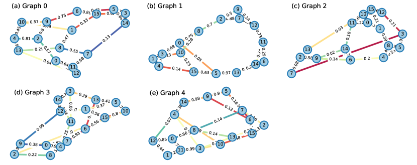
Figure S1: The five $n=16$ w3R graphs used in the MAX-CUT problems. The node ID and the weights are labeled in the corresponding subfigures (a) to (e).

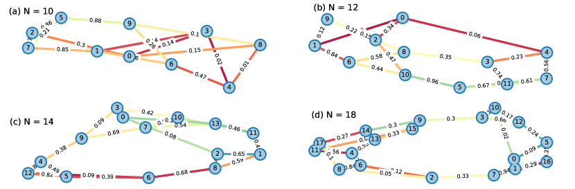
Figure S2: The four w3R graphs with different number of graph sizes (N= 10, 12, 14, 18) used in the MAX-CUT problems. The graph with N=16 is the same one as Fig. S1 (a). The node ID and the weights are labeled in the corresponding subfigures (a) to (d).

VII MAX-CUT problem instances

We test the performance of different optimizers on QAOA of the MAX-CUT problem. All the instances are generated using the random_regular_graph functions in NetworkX package [75]. The codes are also provided in the github repository. The five 16-node weighted graph instances we utilized in the numerical simulations are shown in Fig. S1. The additional four weighted graph instances with different number of nodes are shown in Fig. S2.

VIII Results for more optimizers

We test more choices of different optimizers on Graph 0, to further demonstrate the advantage of DARBO. See Fig. S3 for results with the analytical exact simulation for N = 16 and Fig. S5 for results with finite shot noise. Fig. S4 shows the differences of $r$ and fidelity $f$ between DARBO and other optimizers with different sizes of the graphs. The fidelity of optimized QAOA is defined as the square of the overlap between the exact ground state subspace for MAX-CUT problem (a pair of product state hosting MAX-CUT solution configuration) and the output quantum state of the QAOA circuit. In other words, the fidelity is the probability for measuring QAOA output state to obtain the solution bitstrings with the maximal cut value.

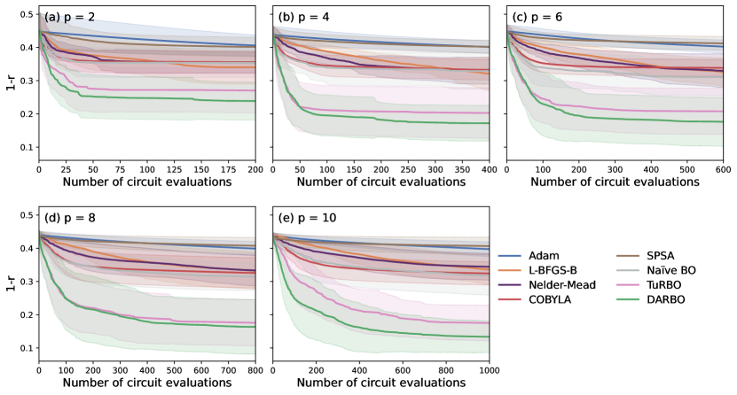
Figure S3: Optimization results for optimizing the MAX-CUT problem in the analytical exact case on Graph 0. The line represents the average $1-r$ across 20 different trials from different initialization parameters, while the shaded area represents the standard deviation across different trials. Each subfigure displays the corresponding results for QAOA of different depths $p$. For each trial, all the optimizers share the same parameter initialization.

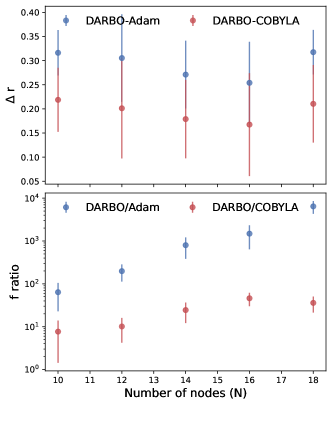
Figure S4: Differences of DARBO, Adam and COBYLA for optimizing the MAX-CUT problem in the analytical exact case on different sizes of the graphs. The average $\Delta r$ and $f$ ratio are computed across 20 different trials from different initialization parameters and plotted as a function of number of nodes ($N$) on the graphs. The error bar is the accumulated standard deviations of two compared optimizers. For each trial, all the optimizers share the same parameter initialization.

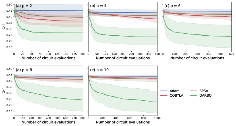
Figure S5: Optimization results for optimizing the MAX-CUT problem on Graph 0 with finite shot noise (shots=200). The line represents the average $1-r$ across 20 different trials from different initialization parameters, while the shaded area represents the standard deviation across different trials. Each subfigure displays the corresponding results for QAOA of different depths $p$. For each trial, all the optimizers share the same parameter initialization.

IX More results on the finite shot noise case

The optimization results in the finite shot noise case are summarized in Fig. S6 for different combinations of shot numbers and the circuit depths.

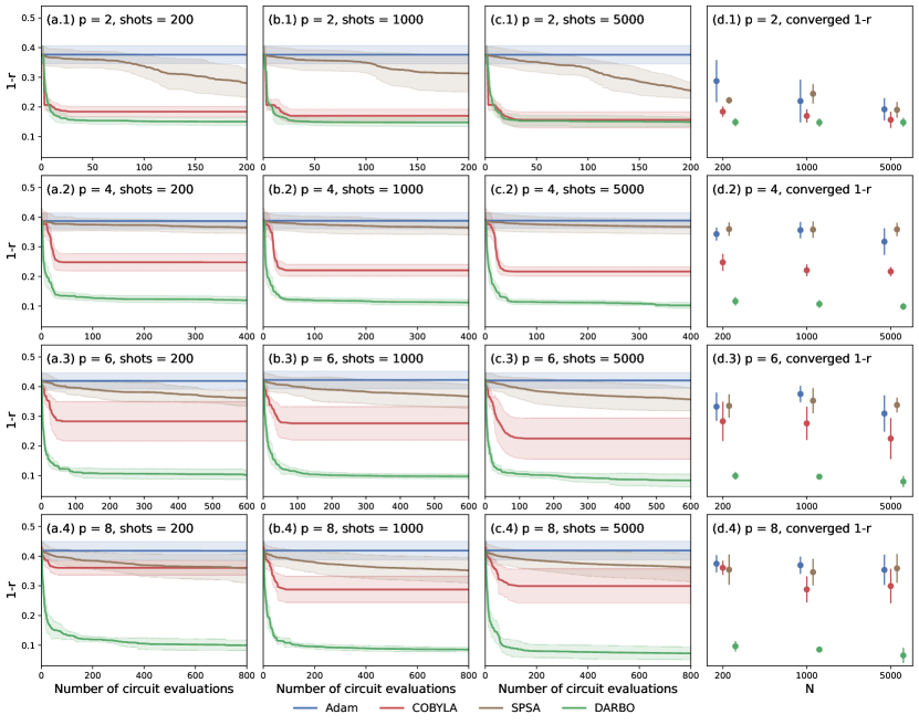
Figure S6: Optimization results over 5 graphs for MAX-CUT problem with shot-noises. The results with different depths ($p=2,4,6,8$) and different numbers of measurement shots (shots=$200,1000,5000$) are shown in the subfigures. The displayed $1-r$ values are the best result from 20 independent optimization trials with different initial guesses, and the shaded area represents the standard deviation across different graph instances. In the subfigures (d.x), the converged $1-r$ values represent the best average 1-r values at the 1000 epochs, where the optimizations are converged.

X Quantum hardware experiments

The superconducting processor we utilized has a $10\times 2$ grid geometry hosting $20$ transmon qubits in total. Typical mean error rates are are $2.4\times 10^{-2}$ for two-qubit gates, $0.2\times 10^{-2}$ for single-qubit gates and $7\times 10^{-2}$ for readout errors. Mean $T_{1}$ and $T_{2}$ time are $23\mu s$ and $5\mu s$, respectively.

The QUBO Hamiltonian used in the real quantum hardware experiments is as follows:

$$C(\mathbf{z})=z_{0}z_{1}-z_{0}z_{2}+z_{0}z_{3}-z_{3}z_{4}.$$ (11)

The underlying graph for this QUBO Hamiltonian is compatible with the geometry of the quantum processor, and thus there is no need to further compile two-qubit gates with extra swap gates which bring more quantum noise otherwise.

In Fig. S7, we show the optimization results when the optimization target is the raw value and the error-mitigated value, respectively. Different from the figure in the main text, we show three values evaluated given the current circuit parameters in the same figure this time. These guidances can help us to have a clear observation of the ultimate optimization performance.

The results not only demonstrate the effectiveness of DARBO as an optimizer for QAOA but also show the enhancement brought by quantum error mitigation. When we run the optimization loop with error-mitigated evaluation, the mitigation results are much closer to the exact results and the fluctuation over different optimization trials is much smaller in the mitigation case.

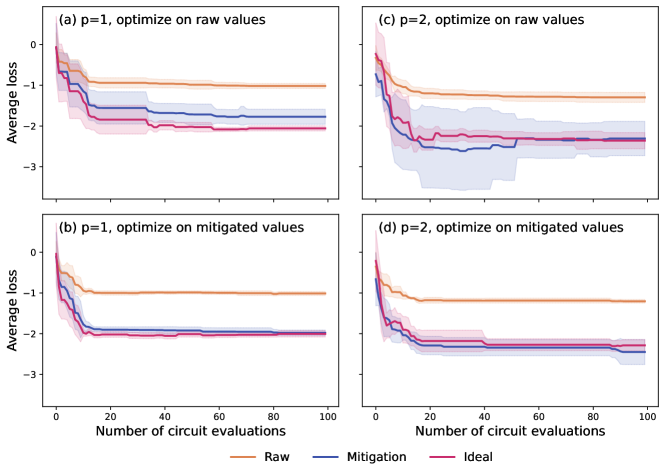
Figure S7: Quantum optimization of a five-variable QUBO problem on real quantum hardware with shots = 10000 for $p$=1 and $2$. The current best parameters at each iteration are determined by optimizing the losses estimated from (a) (c) raw measurements from the quantum processor, and (b) (d) error-mitigated results from the quantum processor. The corresponding raw, mitigation, and ideal losses are evaluated using the current best circuit parameters at each circuit evaluation step. The line is the average optimization trajectory of 5 independent optimization trials while the shaded area represents the standard deviation across these trials.

References

- Schuetz et al. [2022] M. J. Schuetz, J. K. Brubaker, and H. G. Katzgraber, Combinatorial optimization with physics-inspired graph neural networks, Nat. Mach. Intell. 4, 367 (2022).
- Angelini and Ricci-Tersenghi [2022] M. C. Angelini and F. Ricci-Tersenghi, Modern graph neural networks do worse than classical greedy algorithms in solving combinatorial optimization problems like maximum independent set, Nat. Mach. Intell. 5, 29 (2022).
- Boettcher [2023] S. Boettcher, Inability of a graph neural network heuristic to outperform greedy algorithms in solving combinatorial optimization problems, Nat. Mach. Intell. 5, 24 (2023).
- Kadowaki and Nishimori [1998] T. Kadowaki and H. Nishimori, Quantum annealing in the transverse Ising model, Phys. Rev. E. 58, 5355 (1998).
- Farhi et al. [2001] E. Farhi, J. Goldstone, S. Gutmann, J. Lapan, A. Lundgren, and D. Preda, A quantum adiabatic evolution algorithm applied to random instances of an NP-complete problem, Science 292, 472 (2001).
- Johnson et al. [2011] M. W. Johnson, M. H. S. Amin, S. Gildert, T. Lanting, F. Hamze, N. Dickson, R. Harris, A. J. Berkley, J. Johansson, P. Bunyk, E. M. Chapple, C. Enderud, J. P. Hilton, K. Karimi, E. Ladizinsky, N. Ladizinsky, T. Oh, I. Perminov, C. Rich, M. C. Thom, E. Tolkacheva, C. J. S. Truncik, S. Uchaikin, J. Wang, B. Wilson, and G. Rose, Quantum annealing with manufactured spins, Nature 473, 194 (2011).
- Hauke et al. [2020] P. Hauke, H. G. Katzgraber, W. Lechner, H. Nishimori, and W. D. Oliver, Perspectives of quantum annealing: methods and implementations, Rep. Prog. Phys. 83, 054401 (2020).
- Hibat-Allah et al. [2021] M. Hibat-Allah, E. M. Inack, R. Wiersema, R. G. Melko, and J. Carrasquilla, Variational neural annealing, Nat. Mach. Intell. 3, 952 (2021).
- Farhi et al. [2014] E. Farhi, J. Goldstone, and S. Gutmann, A quantum approximate optimization algorithm, Preprint at https://arXiv.org/abs/1411.4028 (2014).
- Zhou et al. [2020] L. Zhou, S.-T. Wang, S. Choi, H. Pichler, and M. D. Lukin, Quantum approximate optimization algorithm: Performance, mechanism, and implementation on near-term devices, Phys. Rev. X. 10, 021067 (2020).
- Harrigan et al. [2021] M. P. Harrigan, K. J. Sung, M. Neeley, K. J. Satzinger, F. Arute, K. Arya, J. Atalaya, J. C. Bardin, R. Barends, S. Boixo, M. Broughton, B. B. Buckley, D. A. Buell, B. Burkett, N. Bushnell, Y. Chen, Z. Chen, Ben Chiaro, R. Collins, W. Courtney, S. Demura, A. Dunsworth, D. Eppens, A. Fowler, B. Foxen, C. Gidney, M. Giustina, R. Graff, S. Habegger, A. Ho, S. Hong, T. Huang, L. B. Ioffe, S. V. Isakov, E. Jeffrey, Z. Jiang, C. Jones, D. Kafri, K. Kechedzhi, J. Kelly, S. Kim, P. V. Klimov, A. N. Korotkov, F. Kostritsa, D. Landhuis, P. Laptev, M. Lindmark, M. Leib, O. Martin, J. M. Martinis, J. R. McClean, M. McEwen, A. Megrant, X. Mi, M. Mohseni, W. Mruczkiewicz, J. Mutus, O. Naaman, C. Neill, F. Neukart, M. Y. Niu, T. E. O’Brien, B. O’Gorman, E. Ostby, A. Petukhov, H. Putterman, C. Quintana, P. Roushan, N. C. Rubin, D. Sank, A. Skolik, V. Smelyanskiy, D. Strain, M. Streif, M. Szalay, A. Vainsencher, T. White, Z. J. Yao, P. Yeh, A. Zalcman, L. Zhou, H. Neven, D. Bacon, E. Lucero, E. Farhi, and R. Babbush, Quantum approximate optimization of non-planar graph problems on a planar superconducting processor, Nat. Phys. 17, 332 (2021).
- Larkin et al. [2022] J. Larkin, M. Jonsson, D. Justice, and G. G. Guerreschi, Evaluation of QAOA based on the approximation ratio of individual samples, Quantum Sci. Technol. 7, 045014 (2022).
- Pelofske et al. [2023] E. Pelofske, A. Bärtschi, and S. Eidenbenz, Quantum annealing vs. QAOA: 127 qubit higher-order Ising problems on NISQ computers, Preprint at https://arXiv.org/abs/2301.00520 (2023).
- Bittel and Kliesch [2021] L. Bittel and M. Kliesch, Training variational quantum algorithms is NP-hard, Phys. Rev. Lett. 127, 120502 (2021).
- Anschuetz [2021] E. R. Anschuetz, Critical points in quantum generative models, Preprint at https://arXiv.org/abs/2109.06957 (2021).
- McClean et al. [2018] J. R. McClean, S. Boixo, V. N. Smelyanskiy, R. Babbush, and H. Neven, Barren plateaus in quantum neural network training landscapes, Nat. Commun. 9, 4812 (2018).
- Ortiz Marrero et al. [2021] C. Ortiz Marrero, M. Kieferová, and N. Wiebe, Entanglement-induced barren plateaus, PRX Quantum 2, 040316 (2021).
- Wang et al. [2021a] S. Wang, E. Fontana, M. Cerezo, K. Sharma, A. Sone, L. Cincio, and P. J. Coles, Noise-induced barren plateaus in variational quantum algorithms, Nat. Commun. 12, 6961 (2021a).
- Arrasmith et al. [2021] A. Arrasmith, M. Cerezo, P. Czarnik, L. Cincio, and P. J. Coles, Effect of barren plateaus on gradient-free optimization, Quantum 5, 558 (2021).
- Verdon et al. [2019] G. Verdon, M. Broughton, J. R. McClean, K. J. Sung, R. Babbush, Z. Jiang, H. Neven, and M. Mohseni, Learning to learn with quantum neural networks via classical neural networks, Preprint at https://arXiv.org/abs/1907.05415 (2019).
- Alam et al. [2020] M. Alam, A. Ash-Saki, and S. Ghosh, Accelerating quantum approximate optimization algorithm using machine learning, in 2020 Design, Automation & Test in Europe Conference & Exhibition (DATE) (IEEE, 2020) pp. 686–689.
- Khairy et al. [2020] S. Khairy, R. Shaydulin, L. Cincio, Y. Alexeev, and P. Balaprakash, Learning to optimize variational quantum circuits to solve combinatorial problems, Proceedings of the AAAI Conference on Artificial Intelligence 34, 2367 (2020).
- Jain et al. [2022] N. Jain, B. Coyle, E. Kashefi, and N. Kumar, Graph neural network initialisation of quantum approximate optimisation, Quantum 6, 861 (2022).
- Shaydulin et al. [2021] R. Shaydulin, K. Marwaha, J. Wurtz, and P. C. Lotshaw, QAOAKit: A toolkit for reproducible study, application, and verification of the QAOA, in 2021 IEEE/ACM Second International Workshop on Quantum Computing Software (QCS), Vol. 50 (IEEE, 2021) pp. 64–71.
- Moussa et al. [2022] C. Moussa, H. Wang, T. Bäck, and V. Dunjko, Unsupervised strategies for identifying optimal parameters in quantum approximate optimization algorithm, EPJ Quantum Technol. 9, 11 (2022).
- Amosy et al. [2022] O. Amosy, T. Danzig, E. Porat, G. Chechik, and A. Makmal, Iterative-Free Quantum Approximate Optimization Algorithm Using Neural Networks, Preprint at https://arXiv.org/abs/2208.09888 (2022).
- Yao et al. [2022] J. Yao, H. Li, M. Bukov, L. Lin, and L. Ying, Monte Carlo Tree Search based Hybrid Optimization of Variational Quantum Circuits, Preprint at https://arXiv.org/abs/2203.16707 (2022).
- Xie et al. [2022] N. Xie, X. Lee, D. Cai, Y. Saito, and N. Asai, Quantum approximate optimization algorithm parameter prediction using a convolutional neural network, Preprint at https://arXiv.org/abs/2211.09513 (2022).
- Tate et al. [2023] R. Tate, M. Farhadi, C. Herold, G. Mohler, and S. Gupta, Bridging classical and quantum with SDP initialized warm-starts for QAOA, ACM Trans. Intell. Syst. Technol. 4, 1 (2023).
- Campos et al. [2021] E. Campos, D. Rabinovich, V. Akshay, and J. Biamonte, Training saturation in layerwise quantum approximate optimization, Phys. Rev. A. 104, L030401 (2021).
- Shaydulin et al. [2022] R. Shaydulin, P. C. Lotshaw, J. Larson, J. Ostrowski, and T. S. Humble, Parameter transfer for quantum approximate optimization of weighted MaxCut, Preprint at https://arXiv.org/abs/2201.11785 (2022).
- Sack et al. [2022] S. H. Sack, R. A. Medina, R. Kueng, and M. Serbyn, Transition states and greedy exploration of the QAOA optimization landscape, Preprint at https://arXiv.org/abs/2209.01159 (2022).
- Mele et al. [2022] A. A. Mele, G. B. Mbeng, G. E. Santoro, M. Collura, and P. Torta, Avoiding barren plateaus via transferability of smooth solutions in a hamiltonian variational ansatz, Physical Review A 106, L060401 (2022).
- Norouzi et al. [2009] M. Norouzi, M. Ranjbar, and G. Mori, Stacks of convolutional restricted boltzmann machines for shift-invariant feature learning, in 2009 IEEE Computer Society Conference on Computer Vision and Pattern Recognition Workshops, CVPR Workshops 2009 (2009) pp. 2735–2742.
- Larocca et al. [2021] M. Larocca, N. Ju, D. Garc’ia-Mart’in, P. J. Coles, and M. Cerezo, Theory of overparametrization in quantum neural networks, Preprint at https://arXiv.org/abs/2109.11676 (2021).
- Kim et al. [2021] J. Kim, J. Kim, and D. Rosa, Universal effectiveness of high-depth circuits in variational eigenproblems, Phys. Rev. Res. 3, 023203 (2021).
- Frazier [2018] P. I. Frazier, A tutorial on Bayesian optimization, Preprint at https://arXiv.org/abs/1807.02811 (2018).
- Eriksson et al. [2019] D. Eriksson, M. Pearce, J. Gardner, R. D. Turner, and M. Poloczek, Scalable global optimization via local Bayesian optimization, in Advances in Neural Information Processing Systems, Vol. 32, edited by H. Wallach, H. Larochelle, A. Beygelzimer, F. d'Alché-Buc, E. Fox, and R. Garnett (Curran Associates, Inc., 2019).
- Letham et al. [2017] B. Letham, B. Karrer, G. Ottoni, and E. Bakshy, Constrained Bayesian optimization with noisy experiments, Preprint at https://arXiv.org/abs/1706.07094 (2017).
- Letham et al. [2020] B. Letham, R. Calandra, A. Rai, and E. Bakshy, Re-examining linear embeddings for high-dimensional Bayesian optimization, in Advances in Neural Information Processing Systems, Vol. 33, edited by H. Larochelle, M. Ranzato, R. Hadsell, M. Balcan, and H. Lin (Curran Associates, Inc., 2020) pp. 1546–1558.
- Yuan [2015] Y.-X. Yuan, Recent advances in trust region algorithms, Math. Program. 151, 249 (2015).
- Powell [1994] M. J. D. Powell, A direct search optimization method that models the objective and constraint functions by linear interpolation, in Advances in Optimization and Numerical Analysis, edited by S. Gomez and J.-P. Hennart (Springer Netherlands, Dordrecht, 1994) pp. 51–67.
- Kingma and Ba [2015] D. P. Kingma and J. Ba, Adam: A method for stochastic optimization, in International Conference on Learning Representations (ICLR), edited by Y. Bengio and Y. LeCun (2015).
- Spall [1998] J. Spall, Implementation of the simultaneous perturbation algorithm for stochastic optimization, IEEE Trans. Aerosp. Electron. Syst. 34, 817 (1998).
- Tibaldi et al. [2022] S. Tibaldi, D. Vodola, E. Tignone, and E. Ercolessi, Bayesian optimization for QAOA, Preprint at https://arXiv.org/abs/2209.03824 (2022).
- Self et al. [2021] C. N. Self, K. E. Khosla, A. W. Smith, F. Sauvage, P. D. Haynes, J. Knolle, F. Mintert, and M. Kim, Variational quantum algorithm with information sharing, Npj Quantum Inf. 7, 116 (2021).
- Tamiya and Yamasaki [2022] S. Tamiya and H. Yamasaki, Stochastic gradient line Bayesian optimization for efficient noise-robust optimization of parameterized quantum circuits, Npj Quantum Inf. 8, 90 (2022).
- Shaffer et al. [2023] R. Shaffer, L. Kocia, and M. Sarovar, Surrogate-based optimization for variational quantum algorithms, Phys. Rev. A 107, 032415 (2023).
- Gelbart et al. [2014] M. A. Gelbart, J. Snoek, and R. P. Adams, Bayesian optimization with unknown constraints, Preprint at https://arXiv.org/abs/1403.5607 (2014).
- Wang et al. [2021b] S. Wang, E. Fontana, M. Cerezo, K. Sharma, A. Sone, L. Cincio, and P. J. Coles, Noise-induced barren plateaus in variational quantum algorithms, Nat. Commun. 12, 6961 (2021b).
- Bravyi et al. [2021] S. Bravyi, S. Sheldon, A. Kandala, D. C. Mckay, and J. M. Gambetta, Mitigating measurement errors in multiqubit experiments, Phys. Rev. A. 103, 042605 (2021).
- Nation et al. [2021] P. D. Nation, H. Kang, N. Sundaresan, and J. M. Gambetta, Scalable mitigation of measurement errors on quantum computers, PRX Quantum 2, 040326 (2021).
- Temme et al. [2017] K. Temme, S. Bravyi, and J. M. Gambetta, Error mitigation for short-depth quantum circuits, Phys. Rev. Lett. 119, 180509 (2017).
- Li and Benjamin [2017] Y. Li and S. C. Benjamin, Efficient variational quantum simulator incorporating active error minimization, Phys. Rev. X. 7, 021050 (2017).
- Eriksson and Jankowiak [2021] D. Eriksson and M. Jankowiak, High-dimensional Bayesian optimization with sparse axis-aligned subspaces, in Uncertainty in Artificial Intelligence (PMLR, 2021) pp. 493–503.
- Nayebi et al. [2019] A. Nayebi, A. Munteanu, and M. Poloczek, A framework for Bayesian optimization in embedded subspaces, in Proceedings of the 36th International Conference on Machine Learning, Proceedings of Machine Learning Research, Vol. 97, edited by K. Chaudhuri and R. Salakhutdinov (PMLR, 2019) pp. 4752–4761.
- Martinez-Cantin et al. [2018] R. Martinez-Cantin, K. Tee, and M. McCourt, Practical Bayesian optimization in the presence of outliers, in International Conference on Artificial Intelligence and Statistics (PMLR, 2018) pp. 1722–1731.
- Fröhlich et al. [2020] L. Fröhlich, E. Klenske, J. Vinogradska, C. Daniel, and M. Zeilinger, Noisy-input entropy search for efficient robust Bayesian optimization, in International Conference on Artificial Intelligence and Statistics (PMLR, 2020) pp. 2262–2272.
- Daulton et al. [2022] S. Daulton, S. Cakmak, M. Balandat, M. A. Osborne, E. Zhou, and E. Bakshy, Robust multi-objective Bayesian optimization under input noise, in International Conference on Machine Learning (PMLR, 2022) pp. 4831–4866.
- Dave et al. [2022] A. Dave, J. Mitchell, S. Burke, H. Lin, J. Whitacre, and V. Viswanathan, Autonomous optimization of non-aqueous li-ion battery electrolytes via robotic experimentation and machine learning coupling, Nat. Commun. 13, 5454 (2022).
- Zhang et al. [2020] Y. Zhang, D. W. Apley, and W. Chen, Bayesian optimization for materials design with mixed quantitative and qualitative variables, Sci. Rep. 10, 1 (2020).
- Cheng et al. [2022] L. Cheng, Z. Yang, B. Liao, C. Hsieh, and S. Zhang, Odbo: Bayesian optimization with search space prescreening for directed protein evolution, Preprint at https://arXiv.org/abs/2205.09548 (2022).
- Zhang et al. [2022] S.-X. Zhang, C.-Y. Hsieh, S. Zhang, and H. Yao, Differentiable quantum architecture search, Quantum Sci. Technol. 7, 045023 (2022).
- Weidinger et al. [2023] A. Weidinger, G. B. Mbeng, and W. Lechner, Error Mitigation for Quantum Approximate Optimization, Preprint at https://arXiv.org/abs/2301.05042 (2023).
- Mockus [2012] J. Mockus, Bayesian approach to global optimization: theory and applications, Vol. 37 (Springer Science & Business Media, 2012).
- Rasmussen and Williams [2006] C. E. Rasmussen and C. K. I. Williams, Gaussian processes for machine learning (MIT Press, Cambridge, MA, 2006).
- Gardner et al. [2018] J. R. Gardner, G. Pleiss, D. Bindel, K. Q. Weinberger, and A. G. Wilson, GPyTorch: Blackbox matrix-matrix gaussian process inference with gpu acceleration, in Advances in Neural Information Processing Systems, edited by S. Bengio, H. Wallach, H. Larochelle, K. Grauman, N. Cesa-Bianchi, and R. Garnett (Curran Associates, Inc., 2018).
- Srinivas et al. [2009] N. Srinivas, A. Krause, S. M. Kakade, and M. Seeger, Gaussian process optimization in the bandit setting: No regret and experimental design, Preprint at https://arXiv.org/abs/0912.3995 (2009).
- Zhang et al. [2023] S.-X. Zhang, J. Allcock, Z.-Q. Wan, S. Liu, J. Sun, H. Yu, X.-H. Yang, J. Qiu, Z. Ye, Y.-Q. Chen, C.-K. Lee, Y.-C. Zheng, S.-K. Jian, H. Yao, C.-Y. Hsieh, and S. Zhang, TensorCircuit: A quantum software framework for the NISQ era, Quantum 7, 912 (2023).
- Abadi et al. [2015] M. Abadi, A. Agarwal, P. Barham, E. Brevdo, Z. Chen, C. Citro, G. S. Corrado, A. Davis, J. Dean, M. Devin, S. Ghemawat, I. Goodfellow, A. Harp, G. Irving, M. Isard, Y. Jia, R. Jozefowicz, L. Kaiser, M. Kudlur, J. Levenberg, D. Mané, R. Monga, S. Moore, D. Murray, C. Olah, M. Schuster, J. Shlens, B. Steiner, I. Sutskever, K. Talwar, P. Tucker, V. Vanhoucke, V. Vasudevan, F. Viégas, O. Vinyals, P. Warden, M. Wattenberg, M. Wicke, Y. Yu, and X. Zheng, TensorFlow: Large-scale machine learning on heterogeneous systems (2015), software available from tensorflow.org.
- Byrd et al. [1995] R. H. Byrd, P. Lu, J. Nocedal, and C. Zhu, A limited memory algorithm for bound constrained optimization, SIAM J. Sci. Comput. 16, 1190 (1995).
- Virtanen et al. [2020] P. Virtanen, R. Gommers, T. E. Oliphant, M. Haberland, T. Reddy, D. Cournapeau, E. Burovski, P. Peterson, W. Weckesser, J. Bright, S. J. van der Walt, M. Brett, J. Wilson, K. J. Millman, N. Mayorov, A. R. J. Nelson, E. Jones, R. Kern, E. Larson, C. J. Carey, İ. Polat, Y. Feng, E. W. Moore, J. VanderPlas, D. Laxalde, J. Perktold, R. Cimrman, I. Henriksen, E. A. Quintero, C. R. Harris, A. M. Archibald, A. H. Ribeiro, F. Pedregosa, P. van Mulbregt, and SciPy 1.0 Contributors, SciPy 1.0: Fundamental Algorithms for Scientific Computing in Python, Nat. Methods 17, 261 (2020).
- Nelder and Mead [1965] J. A. Nelder and R. Mead, A simplex method for function minimization, Comput. J 7, 308 (1965).
- Mayer [2017] A. Mayer, Noisyopt: A Python library for optimizing noisy functions., J. Open Source Softw. 2, 258 (2017).
- Hagberg et al. [2008] A. Hagberg, P. Swart, and D. S Chult, Exploring network structure, dynamics, and function using NetworkX, Tech. Rep. (Los Alamos National Lab.(LANL), Los Alamos, NM (United States), 2008).