Dielectric properties of aqueous electrolytes at the nanoscale

Abstract

Despite the ubiquity of nanoconfined aqueous electrolytes, a theoretical framework that accounts for the nonlinear coupling of water and ion polarization is still missing. We introduce a nonlocal and nonlinear field theory for the nanoscale polarization of ions and water and derive the electrolyte dielectric properties as a function of salt concentration to first order in a loop expansion. Classical molecular dynamics simulations are favorably compared with the calculated dielectric response functions. The theory correctly predicts the dielectric permittivity decrement with rising salt concentration and furthermore shows that salt induces a Debye screening in the longitudinal susceptibility but leaves the short-range water organization remarkably unchanged.

Introduction - The study of nanoconfined electrolytes is exciting both for their ubiquity and for the theoretical challenge they bring [1, 2, 3]. The nanometer scale is the typical confinement size of technological and biological devices, the screening length of low concentrated ionic solutions, as well as the range at which water starts to behave as a discrete molecular medium [4, 5, 6]. The structure of interfacial solutions thus results from a subtle interplay between short-range charge overscreening generated by the solvent [7], ion-ion correlations, water- and ion- surface interactions [8, 9]. The balance between these effects encode many aspects of the double layer structure [10, 11].

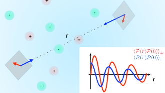
Figure 1: Sketch of the system under study. Water is described as a nonlocal nonlinear continuous dielectric medium and ions as point charges. We evaluate the ionic-strength effect on the water longitudinal $\bm{\mathcal{P}_{\parallel}}$ and transverse $\bm{\mathcal{P}_{\perp}}$ polarization correlations.

The continuous linear description of water used in Poisson-Boltzmann (PB) model cannot capture this complexity. The well-documented decrement of the bulk permittivity of aqueous ionic solutions induced by an increase of the concentration of the salt [12] has been retrieved using nonlinear expansions of a dipolar PB model [13]. But a parameterized nonlocal field theory (FT) for structured solvent to fully describe electrolytes at the nanoscale is missing [14, 15, 16, 17]. For instance, the simple question ”Do electrolytes increase or decrease the range of the longitudinal correlations of water?” is still actively debated [18, 19, 20]. In contrast, the influence of ionic strength on transverse polarization correlations is largely unexplored although it could be of major importance for the interactions between solvated objects [21]. The figure 1 shows an illustration of these questions.

Nonlocal model for water - At the molecular scale, water is a correlated dielectric medium, as illustrated by the wave mode dependence of the correlation tensor of the polarization field $\bm{\mathcal{P}}$ [22, 23]. In Fourier space, the longitudinal susceptibility of water, ${\chi^{\rm w}_{\parallel}(q)=\beta\langle\bm{\mathcal{P}}_{\parallel}(\mathbf{q})\cdot\bm{\mathcal{P}}_{\parallel}(-\mathbf{q})\rangle/\epsilon_{0}}$, - with $\beta$ the inverse temperature, $\epsilon_{0}$ the vacuum permittivity, $\bm{\mathcal{P}}_{\parallel}$ the longitudinal part of the polarization, $\mathbf{q}$ the wave vector - exhibits an overresponse peak around $q$=3Å^-1. This structured response characterizes a charge overscreening at short range, induced by the layering of water molecules organized by the water hydrogen bond network [22]. The transverse susceptibility ${\chi^{\rm w}_{\perp}(q)=\beta\langle\bm{\mathcal{P}}_{\perp}(\mathbf{q})\cdot\bm{\mathcal{P}}_{\perp}(-\mathbf{q})\rangle/\epsilon_{0}}$, with $\bm{\mathcal{P}}_{\perp}$ the transverse part of the polarization - exhibits a Lorentzian decay at low $q$ [23].

Continuum nonlocal electrostatics provides a useful framework to describe correlated fluids [24, 25, 26]. The electrostatic energy of the fluid $\mathcal{U}_{\rm el}$ can be written as a Gaussian functional of $\bm{\mathcal{P}}$,

$$\mathcal{U}_{\rm el}[\bm{\mathcal{P}}]=\frac{1}{2}\int d\mathbf{r}d\mathbf{r}^{\prime}\frac{\nabla\cdot\bm{\mathcal{P}}(\mathbf{r})\nabla\cdot\bm{\mathcal{P}}(\mathbf{r}^{\prime})}{4\pi\epsilon_{0}|\mathbf{r}-\mathbf{r}^{\prime}|}+\mathcal{U}^{\rm G}_{\rm conf}[\bm{\mathcal{P}}].$$ (1)

The first term corresponds to the bare Coulomb interactions between the partial charges $-\nabla\cdot\bm{\mathcal{P}}(\mathbf{r})$ of the fluid. The phenomenological configuration energy $\mathcal{U}^{\rm G}_{\rm conf}[\bm{\mathcal{P}}]$, where the subscript G stands for Gaussian, can be made explicit using a Landau-Ginzburg expansion [27] such as,

$$\mathcal{U}^{\rm G}_{\rm conf}[\bm{\mathcal{P}}] = \frac{1}{2\epsilon_{0}}\int d\mathbf{r}\Big{[}K\bm{\mathcal{P}}(\bm{r})^{2}+\kappa_{l}(\bm{\nabla}\cdot\bm{\mathcal{P}}(\bm{r}))^{2}$$ (2)

$$+ \kappa_{t}(\bm{\nabla}\times\bm{\mathcal{P}}(\bm{r})^{2}+\alpha(\bm{\nabla}(\bm{\nabla}\cdot\bm{\mathcal{P}}(\bm{r})))^{2}\Big{]}\,$$

expanded up to the first spatial derivative for the transverse terms (term in $\kappa_{t}$) and up to the second one for the longitudinal ones (terms in $\kappa_{l}$ and $\alpha$). Eq. (2) has been shown to capture the main features of dielectric properties of water at the nanoscale [28, 6]. The polarization susceptibility $\chi^{\rm w}$, obtained by inversion of Eq. (1), can be decomposed in Fourier space in a longitudinal $\chi_{\parallel}^{\rm w}$ and a transverse $\chi_{\perp}^{\rm w}$ response using isotropy and homogeneity of the system, such that $\chi_{ij}(\mathbf{q})=\chi^{\rm w}_{\parallel}(q)q_{i}q_{j}/q^{2}+\chi^{\rm w}_{\perp}(q)(\delta_{ij}-q_{i}q_{j}/q^{2})$, with $(i,j)=(x,y,z)$. Their expressions follow from Eq. (2) as

$$\chi_{\parallel}^{\rm w}(q)=\frac{1}{1+K+\kappa_{l}q^{2}+\alpha q^{4}},\quad\chi_{\perp}^{\rm w}(q)=\frac{1}{K+\kappa_{t}q^{2}}.$$ (3)

$\chi^{\rm w}_{\parallel}$ is associated with a decay $\lambda_{l}$ and an oscillating $\lambda_{o}$ correlation length and $\chi^{\rm w}_{\perp}$ with a transverse correlation length $\lambda_{t}$ for which explicit expressions are given in S1.1. The bulk permittivity $\epsilon_{w}$ of water is defined as ${\epsilon_{w}=(1-\chi_{\parallel}(0))^{-1}=1+1/K}$ [22]. Figure 2 shows $\chi_{\parallel}^{\rm w}$ and $\chi_{\perp}^{\rm w}$ (blue line) for which Eq. (2) has been parameterized to reproduce MD simulated TIP4p/$\epsilon$ water [29]. Details are provided in S1.1 and the values of the Landau-Ginzburg parameters ($K$, $\kappa_{l}$, $\kappa_{t}$, $\alpha$ ) are given in the caption of Fig. 2.

A term scaling like $\bm{\mathcal{P}}^{4}$, unfavorable to large values of the polarization field, can be added to correct the Gaussian model. The configuration energy [27] thus reads:

$$\mathcal{U}_{\rm conf}[\bm{\mathcal{P}}] = \frac{1}{2\epsilon_{0}}\int d\mathbf{r}\Big{[}\gamma(\bm{\mathcal{P}}(\bm{r})^{2}+P_{0}^{2})^{2}+\kappa_{l}(\bm{\nabla}\cdot\bm{\mathcal{P}}(\bm{r}))^{2}$$ (4)

$$+ \kappa_{t}(\bm{\nabla}\times\bm{\mathcal{P}}(\bm{r}))^{2}+\alpha(\bm{\nabla}(\bm{\nabla}\cdot\bm{\mathcal{P}}(\bm{r})))^{2}\Big{]}$$

and takes into account the saturation of water polarization in the presence of strong fields [30, 31, 32], in addition to nanometric correlations. Such a medium presents a threshold saturation, $P_{0}$, between a linear response ($|\bm{\mathcal{P}}|\ll P_{0}$) and a saturation response ($|\bm{\mathcal{P}}|\gg P_{0}$) regime. We impose $P_{0}=\sqrt{K/2\gamma}$ so that the quadratic local terms in Eq. (2) - $K\bm{\mathcal{P}}^{2}$ - and Eq. (4) - $2\gamma P_{0}^{2}\bm{\mathcal{P}}^{2}$ become equal. Thus, in the low-field regime, the two models are associated with the same nonlocal properties [32] and $\gamma$ remains the only degree of freedom tuning the saturation threshold.

In this letter, we compute the Gibbs free energy and the nonlocal dielectric susceptibility of an aqueous electrolyte for which water is modeled by Eq. (2). We perform MD simulations and compare the Gaussian model to a simulated system. We include saturation effects using Eq. (4) including the one-loop expansion. We determine the effect of the ionic strength on the bulk permittivity, the longitudinal and transverse water correlations. Finally, we identify the essential building blocks to construct a field theory modeling electrolytes at the nanoscale.

Gaussian model for electrolytes - We consider an electrolyte with $N_{+}$ punctual cations of charge $e$ and $N_{-}$ punctual anions of charge $-e$ solvated in water modeled with Eq. (2). The ionic charge density reads $\rho(\mathbf{r})=\Sigma_{i=1}^{N+}e\delta(\mathbf{r}-\mathbf{r}_{i}^{+})-\Sigma_{j=1}^{N-}e\delta(\mathbf{r}-\mathbf{r}_{j}^{-})$. In the canonical ensemble, the partition function of the system can be written as

$$\mathcal{Z}^{\rm G}=\frac{1}{N_{+}!}\frac{1}{N_{-}!}\left[\prod_{i=1}^{N+}\int d\mathbf{r}_{i}^{+}\right]\left[\prod_{j=1}^{N-}\int d\mathbf{r}_{j}^{-}\right]$$

$$\times\int\mathcal{D}[\bm{\mathcal{P}}]e^{-\beta\mathcal{U}^{\rm G}_{\rm conf}[\bm{\mathcal{P}}]}e^{-\frac{\beta}{2}\int d\mathbf{r}d\mathbf{r}^{\prime}\rho_{\rm tot}(\mathbf{r})v(\mathbf{r}-\mathbf{r}^{\prime})\rho_{\rm tot}(\mathbf{r}^{\prime})}\,$$ (5)

with $\rho_{\rm tot}(\mathbf{r})=\rho(\mathbf{r})-\nabla\cdot\bm{\mathcal{P}}(\mathbf{r})$ and $v(\mathbf{r})=1/4\pi\epsilon_{0}|\mathbf{r}|$. $\mathcal{Z}^{\rm G}$ includes the configurational degrees of freedom of the solvent and the Coulomb interactions between free and partial charges. Performing a Hubbard-Stratonivich transformation to get rid of the long-range potential $v$ and switching to the grand canonical ensemble for a more tractable expression, we obtain the grand-canonical ensemble partition function, ${\Xi^{\rm G}=\int\mathcal{D}[\bm{\mathcal{P}}]\,\mathcal{D}[\Psi]e^{-\beta F_{u}^{\rm G}[\bm{{\mathcal{P}}},\Psi]}}$ [13]. The action $F^{\rm G}_{u}[{\bm{\mathcal{P}}},\Psi]$ is a functional of ${\bm{\mathcal{P}}}$ and of the electrostatic potential $\Psi$. Assuming a 1:1 electrolyte and an ionic density $n$, we find:

$$F_{u}^{\rm G}[{\bm{\mathcal{P}}},\Psi] = \mathcal{U}^{\rm G}_{\rm conf}[\bm{\mathcal{P}}]-\int d\mathbf{r}\Big{(}\frac{\epsilon_{0}}{2}(\nabla\Psi)^{2}-\Psi\nabla\cdot\bm{\mathcal{P}}$$ (6)

$$- \frac{2n}{\beta}\cosh(\beta\Psi e)\Big{)}.$$

See S1.2 for a detailed derivation. The free energy $\mathcal{F}^{\rm G}$ of the system follows from $\mathcal{F}^{\rm G}=-k_{B}T\rm{ln}\Xi^{\rm G}$. The associated susceptibility is a 4$\times$4 matrix defined as the inverse of the second functional derivative of $\mathcal{F}^{\rm G}$ as

$$\left(\begin{array}[]{cc}\epsilon_{0}\chi^{\rm G}&\chi^{\rm G}_{P,\psi}\\ \chi^{\rm G}_{\psi,P}&\chi^{\rm G}_{\psi,\psi}/\epsilon_{0}\end{array}\right) ({\mathbf{r}_{1}-\mathbf{r}_{2}})=$$ (12)

$$\left(\begin{array}[]{cc}\frac{\delta^{2}F_{u}^{\rm G}(\bm{P},\Psi)}{\delta\mathcal{P}_{i}(\mathbf{r}_{1})\delta\mathcal{P}_{j}(\mathbf{r}_{2})}&\frac{\delta^{2}F_{u}^{\rm G}(\bm{P},\Psi)}{\delta\mathcal{P}_{i}(\mathbf{r}_{1})\delta\Psi(\mathbf{r}_{1})}\\ \frac{\delta^{2}F_{u}^{\rm G}(\bm{P},\Psi)}{\delta\Psi(\mathbf{r}_{1})\delta\mathcal{P}_{j}(\mathbf{r}_{2})}&\frac{\delta^{2}F_{u}^{\rm G}(\bm{P},\Psi)}{\delta\Psi(\mathbf{r}_{1})\delta\Psi(\mathbf{r}_{2})}\end{array}\right)^{-1}$$

where ($\bm{P},\psi$) are the mean fields minimizing the action $F^{\rm G}_{u}$. They both vanish (See S1.3). As the medium is homogeneous and isotropic, the 2-point susceptibility is a function of the distance ${\mathbf{r}_{1}-\mathbf{r}_{2}}$. We focus here on the polarization susceptibility, which is written in Fourier space as $\chi^{\rm G}_{ij}(q)=\chi^{\rm G}_{\parallel}(q)q_{i}q_{j}/q^{2}+\chi^{\rm G}_{\perp}(q)(\delta_{ij}-q_{i}q_{j}/q^{2})$.

Figure 2: Dielectric susceptibility for electrolytes. (a) Gaussian longitudinal susceptibility $\chi_{\parallel}^{\rm G}$ - Eq. (13) - as a function of $q$ for water and solutions of increasing salt concentration. The arrow indicates the increase of the peak maximum with an increase of the concentration. (b) Transverse susceptibility $\chi_{\perp}^{\rm G}=\chi_{\perp}^{\rm w}$ given by Eq (3) as a function of $q$, which is identical for water and electrolytic solutions. The parameter values of the FT model given in Eq. (2) are $K$= 1/76, $\kappa_{l}$= -0.218 Å^-2, $\alpha$=0.012 Å^-4 and $\kappa_{t}$=0.013 Å^-2.

The longitudinal term reads

$$\chi^{\rm G}_{\parallel}(q)=\frac{\frac{\epsilon_{w}}{\lambda_{D}^{2}}+q^{2}}{\left(\frac{\epsilon_{w}}{\lambda_{D}^{2}}+q^{2}\right)(K+\kappa_{l}q^{2}+\alpha q^{4})+q^{2}},$$ (13)

with the Debye length $\lambda_{D}=\sqrt{\epsilon_{0}\epsilon_{w}/2\beta ne^{2}}$. See S1.4 for details. Fig. (2) a) shows $\chi_{\parallel}^{\rm G}(q)$ for increasing salt concentration $c=n/\mathcal{N}_{a}$, where $\mathcal{N}_{a}$ is the Avogadro number. The Gaussian model predicts an enhancement of the water ordering with an increase of $c$, as indicated by the magnitude increase of the peak at $q$=3 Å^-1. This can be understood as follows. In the nonlocal Gaussian framework, an ion, located in $r=0$ generates the electrostatic potential, $1/4\pi\epsilon_{0}\epsilon_{w}r$, and an extra potential decaying on a range $\lambda_{l}$ and oscillating around zero with a period $\lambda_{o}$ [33]. This oscillating landscape leads to the organization of the charges and to longer-range correlations that increase with the salt concentration until a nonphysical crystallization of the system occurs, corresponding to a divergence of $\chi_{\parallel}^{\rm G}(q)$. See S1.4 for details. In contrast, for a very diluted solution $\lambda_{D}\rightarrow\infty$ (see green line in Fig. 2), the longitudinal susceptibility can be approximated as $\chi_{\parallel}^{\rm G}(q)\approx(\epsilon_{w}/\lambda_{D}^{2}+q^{2})/(K(\epsilon_{w}/\lambda_{D}^{2}+q^{2})+q^{2})+\chi^{\rm w}_{\parallel}(q)$, the sum of the Debye response function for an homogeneous electrolyte and the pure water spectrum. The Debye length $\lambda_{D}$ and the water-water correlation lengths $\lambda_{l}$ and $\lambda_{o}$ do not couple. The Debye contribution dominates for the low $q$ limit and generates a Lorentzian decay as seen in Fig.(2). The transverse susceptibility $\chi^{\rm G}_{\perp}(q)$ is unaffected by the presence of salt and obeys $\chi_{\perp}^{\rm G}(q)$=$\chi_{\perp}^{\rm w}(q)$. Indeed, the coupling between the salt and the solvent occur via the Coulomb interactions and involves only the longitudinal part of the polarization as seen in Eq. (Dielectric properties of aqueous electrolytes at the nanoscale). Finally, we note that the Gaussian model predicts that the dielectric bulk properties of electrolyte solutions $\chi_{\parallel}^{\rm G}(0)=\chi_{\perp}^{\rm G}(0)=1/K$ are independent of the salt concentration.

Comparison with MD simulations - To check the validity of the Gaussian model, we compare its predictions with the dielectric properties of simulated solutions of NaCl in TIP4p/$\epsilon$ water for concentrations $c$ up to 1.5 mol.L^-1 [29, 34]. Simulation details are given in S2. We compute the bulk permittivity and plot $\epsilon(c)$ in Fig. 3 (a). We observe a linear decay, which is not described by the Gaussian model that predicts a constant permittivity. The susceptibilities $\chi_{\perp}^{\rm MD}(q)$ and $\chi_{\parallel}^{\rm MD}(q)$ are shown in Fig 3 (b) and (c) for $c$=0.15 mol.L^-1 - $\lambda_{D}$=7.8 Å-, $c$=0.75 mol.L^-1 - $\lambda_{D}$=3.5 Å-, and $c$=1.5 mol.L^-1 - $\lambda_{D}$=2.5 Å. The blue markers show the response for pure water. We observe a decay of the bulk value $\chi^{\rm MD}_{\perp}(0)$ for an increasing concentration, which is not captured by the Gaussian model. In the longitudinal case, we see a very low coupling between the Debye contribution (Lorentzian decay for $q\leq$2 Å^-1) and the spectrum of water ($q>$2 Å^-1), which remains almost unperturbed. A concentration increase induces a decrease and a flattening of the pseudo resonant peak. The MD results indicate thus an effect of the salt opposite to the Gaussian model predictions that appears at much higher concentration.

A Nonlinear model for the solvent - To get a better agreement between FT and MD simulations, we consider the nonlinear configuration energy $\mathcal{U}_{\rm conf}$ in Eq. (4). We derive the inverse susceptibility of the system to first order in a loop expansion [13]. The grand partition function obeys ${\Xi=\int\mathcal{D}[\bm{\mathcal{P}}]\,\mathcal{D}[\Psi]e^{-\beta F_{u}[\bm{{\mathcal{P}}},\Psi]}}$ with $F_{u}[\bm{\mathcal{P}},\Psi]$ obtained by replacing $\mathcal{U}^{\rm G}_{\rm conf}$ by $\mathcal{U}_{\rm conf}$ in Eq. (6). The mean fields ($\bm{P},\psi$) still vanish, see S1.3. The action $F_{u}$ is expanded up to the second order in $(\bm{\mathcal{P}},\Psi)$ around the mean field solution, $F_{u}[\bm{\mathcal{P}},\Psi]\approx F_{u}[{\bm{P}},\psi]+1/2\int d\mathbf{r}d\mathbf{r}^{\prime}(\delta\bm{P}(\mathbf{r}),\delta\psi(\mathbf{r}))\cdot F_{u}^{(2)}({\bm{P}},\psi)\cdot(\delta\bm{P}(\mathbf{r^{\prime}}),\delta\psi(\mathbf{r}^{\prime}))$, with $F_{u}^{(2)}$ the second functional derivative of $F_{u}$ with respect to $(\bm{\mathcal{P}},\Psi)$ and $\delta\bm{P}=\bm{\mathcal{P}}-{\bm{P}}$, $\delta\psi=\Psi-\psi$. See S1.7 for details. The free energy is then written as $\mathcal{F}\approx F_{u}[{\bm{P}},\psi]+{\rm Tr}{\rm ln}(\beta F_{u}^{(2)}[{\bm{P}},\psi])/\beta$. The inverse susceptibility follows as $\chi^{-1}(\mathbf{r}_{1}-\mathbf{r}_{2})=\chi^{-1,{\rm G}}(\mathbf{r}_{1}-\mathbf{r}_{2})+\chi^{-1,1}(\mathbf{r}_{1}-\mathbf{r}_{2})$, with the one loop correction term $\chi^{-1,1}(\mathbf{r}_{1}-\mathbf{r}_{2})$ defined as:

$$\chi^{-1,1}_{i,j}(\mathbf{r}_{1}-\mathbf{r}_{2})=\frac{1}{2\beta}\frac{\delta^{2}{\rm Tr}\ln\beta F_{u}^{(2)}}{\delta\mathcal{P}_{i}(\mathbf{r}_{1})\delta\mathcal{P}_{j}(\mathbf{r}_{2})}({\bm{P}},\psi).$$ (14)

$\chi^{-1,{\rm G}}$ is the inverse of the Gaussian susceptibility $\chi^{\rm G}$ given in Eq. (13). Performing the field derivatives and calculating the trace in Eq. (14), one obtains

$$\chi_{i,j}^{-1,1}(\mathbf{r}_{1}-\mathbf{r}_{2})=\delta K\delta(\mathbf{r}_{1}-\mathbf{r}_{2})\delta_{ij}\quad{\rm with}$$

$$\delta K = \frac{20\gamma\epsilon_{0}}{3\beta}\left(\chi^{\rm G}_{\parallel}(r_{c})+2\chi^{\rm G}_{\perp}(r_{c})\right).$$ (15)

The first order correction of the susceptibility is purely local and proportional to $\gamma$, which tunes the saturation regime of the model, and depends on the Debye length via $\chi^{\rm G}_{\parallel}$. The cutoff distance $r_{c}$ has been introduced to get rid of the divergence of $\chi^{\rm G}$ in $r=0$. See S1.7 for a detailed derivation and expressions of $\chi^{\rm G}_{i}(r_{c})$, $i=\parallel,\perp$. It can be written in Fourier space as ${\chi_{ij}^{-1,1}(\mathbf{q})=\delta Kq_{i}q_{j}/q^{2}+\delta K(\delta_{ij}-q_{i}q_{j}/q^{2})}$.

The corrected permittivity, $\epsilon=1+1/(K+\delta K)$ depends now on $\lambda_{D}$ and thus on the salt concentration. $\delta K$ is expanded linearly in $c$ as ${\delta K(c)=\delta K_{w}+\delta K_{c}c+\tau(c^{2})}$, where $\delta K_{w}$ is the one-loop expanded correction to $K$ for pure water and $\delta K_{c}c$ is the correction induced by the salt at linear order. Their expressions are derived in S1.8. Setting $\delta K_{w}$ to zero as it is included in the fitted value of $K$, and performing a linear expansion in $c$ of $\epsilon(c)=1+1/(K+\delta K_{c}c)$, we find the permittivity,

$$\epsilon(c) = \epsilon_{w}-\frac{\delta K_{c}}{K^{2}}c,\quad{\rm with}$$ (16)

$$\delta K_{c} = \frac{5\gamma\mathcal{N}_{a}e^{2}(\epsilon_{w}-1)^{2}}{24\pi\epsilon_{w}^{2}}\frac{(4\pi^{2}\lambda_{l}^{2}+\lambda_{o}^{2})(4\pi^{2}\lambda_{l}^{2}+5\lambda_{o}^{2})}{\lambda_{l}\lambda_{o}^{4}}$$

The permittivity decrement is here expressed as a function of the bulk permittivity and the intrinsic longitudinal correlation lengths of the fluid.

Susceptibility kernels for electrolytes - We now compare the polarization susceptibilities obtained from MD simulations and the nonlinear FT models. Figure 3 (a) shows $\epsilon(c)$, Eq. (16), for a value of $\gamma$ adjusted to reproduce the MD data and given in the caption of Fig 3.

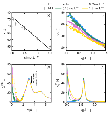
Figure 3: Comparison of FT derived and MD simulated response functions of electrolytes. (a) Bulk permittivity as a function of $c$. The field theory expression is given in Eq. (16) and plotted for $\gamma$=0.08 Å⁴.e^-2, (b) Transverse permittivity - FT expression given in Eq (17), (c) MD simulated longitudinal susceptibility $\chi_{\parallel}^{\rm MD}$, (d) conjectured expression of the longitudinal susceptibility $\chi_{\parallel}^{\rm FT}$ given in Eq. (18). Susceptibilities are plotted as function of $q$ for pure water and electrolytes of increasing concentration.

The one-loop corrected transverse response,

$$\chi^{\rm FT}_{\perp}(q)=\frac{1}{K+\delta K_{c}c+\kappa_{t}q^{2}},$$ (17)

is plotted in Fig. 3 (b) for $c$=0, 0.15, 0.75, 1.5 mol.L^-1 and shows very good agreement with simulations. The one-loop expanded longitudinal susceptibility is obtained by replacing $K$ by ${K+\delta K_{c}c}$ in Eq. (13). Similarly to the Gaussian model, it foresees an enhancement of the longitudinal correlations (See S1.9) and thus fails to reproduce MD data.

Guided by the absence of coupling between the Debye wavelength and the water-water correlation spectrum illustrated by the simulations, we propose an ad hoc longitudinal susceptibility as follows:

$$\chi^{\rm FT}_{\parallel}(q) = \frac{\frac{\epsilon_{w}}{\lambda_{D}^{2}}+q^{2}}{(K+\delta K_{c}c)(\frac{\epsilon_{w}}{\lambda_{D}^{2}}+q^{2})+q^{2}}$$ (18)

$$+ \frac{1}{1+K+\delta K_{c}c+\kappa_{l}q^{2}+\alpha q^{4}}.$$

The first term corresponds to the susceptibility of an homogeneous electrolyte associated with the corrected permittivity $\epsilon(c)$ given in Eq. (16). The second term corresponds to the nonlocal susceptibility of pure water associated with this corrected permittivity. We plot $\chi^{\rm FT}_{\parallel}(q)$ for $c$=0, 0.15, 0.75, 1.5 mol.L^-1 in Fig. 3 (d). It reproduces well MD data as it presents a Lorentzian decay at low $q$ and a flattening of the pseudo-resonant peak at $q$=3 Å^-1 for an increase of the salt concentration.

Discussion - In this work, we have derived analytic expressions for the dielectric response functions of electrolytes at the nanoscale. To do so, we have compared susceptibilities calculated from a FT including nonlocal and nonlinear behavior of water and susceptibilities derived with classical MD simulations. We have thus identified the key effects of the salt on the medium organization. For the longitudinal modes, we highlight two length scales that do not couple to each other: at small wave-modes, $q\leq$2 Å^-1, the medium can be described as homogeneous with a permittivity $\epsilon(c)$ decaying with the salt concentration. This corresponds to long-range interactions for which the Debye screening occurs. At larger $q$, the water longitudinal susceptibility is similar to the one of pure water but associated with a corrected permittivity $\epsilon(c)$. These two decoupled $q$-domains could indicate two ”types” of water molecules that are spatially separated: the one solvating ions polarize in a saturated manner in response to the ionic field, creating an ”electrically dead” solvation shell [13]. Outside of this hydration shell, the molecular water organization remarkably is unaffected by the ions, as recently predicted by machine learning based simulations [20]. We note that local nonlinear models of water also foresee two response regimes (a linear response at low electrostatic excitation and a saturated response at high excitation) with an abrupt switch between the two regimes [35]. Moreover, our work reveals the absence of coupling between salt screening and transverse polarization modes of water. This surprising result could have important consequences on the interactions between objects immersed in electrolytes [36] that were assumed to be screened in any circumstances. This study gives a clear picture of the nature and the range effect of the salt on water organization at the nanoscale for unconfined solutions. This paves the way to develop a field theory describing the properties of nanoconfined electrolytes.

HB thanks H. Orland for fruitful discussions. H.B. acknowledges funding from Humboldt Research Fellowship Program for Experienced Researchers. M.B. acknowledges support by Deutsche Forschungsgemeinschaft, Grant No. CRC 1349, Code No. 387284271, Project No. C04. This work was funded by the Deutsche Forschungsgemeinschaft (DFG, German Research Foundation) in project GRK 2662 - 434130070.

References

- [1] O. Björneholm, M. H. Hansen, A. Hodgson, L-M. Liu, D. T. Limmer, A. Michaelides, P. Pedevilla, J. Rossmeisl, H. Shen, G. Tocci, E. Tyrode, M.-M. Walz, J. Werner, and H. Bluhm. Water at interfaces. Chem. Rev., 116:7698–7726, 2016.
- [2] N. Kavokine, R. R. Netz, and L. Bocquet. Fluids at the nanoscale: From continuum to subcontinuum transport. Annual Review of Fluid Mechanics,, 53:377–410, 2020.
- [3] G. Gonella, E. H. G. Backus, Y. Nagata, J. D. Bonthuis, P. Loche, A. Schlaich, R. R. Netz, A. Künle, I. A. McCrum, M. T. M. Kopper, M. Wolf, B. Winter, G. Meijer, R. Kramer Campen, and M. Bonn. Water at charged interfaces. Nature Reviews Chemistry, 5:466–485, 2021.
- [4] A. Schlaich, E. W. Knapp, and R. R. Netz. Water dielectric effects in planar confinement. Phys. Rev. Lett., 117:048001.
- [5] L. Fumagalli, A. Esfandiar, R. Fabregas, S. Hu, P. Ares, A. Janardanan, Q. Yang, B. Rhada, T. Tanagushi, K. Watanabe, G. Gomila, K. S. Novoselov, and A. K. Geim. Anomalous low dielectric constant of confined water. Science, 360:1339–1342, 2018.
- [6] G. Monet, F. Bresne, A. Kornyshev, and H. Berthoumieux. Nonlocal dielectric response of water in nanoconfinement. Phys. Rev. Lett., 126:216001, 2021.
- [7] S. Chen, Y. Itoh, T. Masuda, S. Shimizu, J. Zhao, J. Ma, S. Nakamura, K. Okuro, H. Noguchi, K. Uosaki, and T. Aida. Subnanoscale hydrophobic modulation of salt bridges in aqueous media. Science, 348:555–559, 2015.
- [8] A. Tuladar, S. Dewan, S. Pezzotti, F. S. Brigiano, F. Creazzo, M.-P. Gaigeot, and E. Borguet. Ions tune interfacial water structure and modulate hydrophobic interactions at silica surfaces. J. Am. Chem. Soc., 142:6991–7000, 2020.
- [9] A. Robert, H. Berthoumieux, and M.-L. Bocquet. Coupled interactions at the ionic graphene/water interface. Phys. Rev. Lett., 157:184801, 2023.
- [10] D. Martin-Jimenez, E. Chacon, P. Tarazona, and R. Garcia. Atomically resolved three-dimensional structures of electrolyte aqueous solutions near a solid surface. Nat. Commun., 7:1–7, 2016.
- [11] S. S. Lee, A. Koishi, I. C. Bourg, and P. Fenter. Ion correlations drive charge overscreening and heterogeneous nucleation at solid–aqueous electrolyte interfaces. Proc. Natl. Acad. Sci. USA, 118(32):e2105154118, 2021.
- [12] J. B. Hasted, D. M. Ritson, and C. H. Collie. Dielectric properties of aqueous ionic solutions. part i and ii. J. Chem. Phys., 16:1–21, 1948.
- [13] A. Levy, D. Andelman, and H. Orland. Dielectric constant of ionic solutions: A field-theory approach. Phys. Rev. Lett., 108:227801, 2012.
- [14] F. Paillusson and R. Blossey. Slits, plates, and poisson-boltzmann theory in a local formulation of nonlocal electrostatics. Phys. Rev. E, 82:052501, 2010.
- [15] D. Ben-Yaakov, D. Andelman, R. Podgornik, and D. Harries. Ion-specific hydration effects: Extending the poisson-boltzmann theory. Current Opinion in Colloid & Interface Science, 16:542–550, 2011.
- [16] R. Blossey and R. Podgornick. Continuum theories of structured dielectrics. EPL, 139:27002, 2022.
- [17] R. Blossey and R. Podgornick. A comprehensive continuum theory of structured liquids. J. Phys. A Math. Theor., 56:025002, 2023.
- [18] A. W. Omta, M. F. Kropman, S. Woutersen, and H. J. Bakker. Negligible effect of ions on the hydrogen-bond structure in liquid water. Science, 301:347–349, 2003.
- [19] Y. Chen, H. I. Okur, N. Gomopoulos, C. Macias-Romero, P. S. Cremer, P. B. Petersen, G. Tocci, D. M. Wilkins, C. Liang, M. Ceriotti, and S. Roke. Electrolytes induce long-range orientational order and free energy changes in the H-bond network of bulk water. Sci. Adv., 2:e1501891, 2016.
- [20] C. Zhang, S. Yue, A. Z. Panagiotopoulos, M. L. Klein, and X. Wu. Dissolving salt is not equivalent to applying pressure on water. Nat. Commun., 13:822, 2022.
- [21] T. Schoeger, B. Spreng, G.-L. Ingold, P. A. Maia Neto, and S. Reynaud. Universal casimir interaction between350 two dielectric spheres in salted water. Phys. Rev. Lett., 128:230602, 2022.
- [22] P. A. Bopp, A. A. Kornyshev, and G. Sutmann. Static Nonlocal Dielectric Function of Liquid Water. Phys. Rev. Lett., 76:1280–1283, 1996.
- [23] P. A. Bopp, A. A. Kornyshev, and G. Sutmann. Frequency and wave-vector dependent dielectic function of water: Collective modes and relaxation spectra. J. Chem. Phys., 109:1940–1958, 1998.
- [24] A. A. Kornyshev. On the non-local electrostatic theory of hydration force. Journal of Electroanalytical Chemistry and Interfacial Electrochemistry, 204(1-2):79–84, June 1986.
- [25] M. V. Basilevsky and D. F. Parsons. Nonlocal continuum solvation model with exponential susceptibility kernels. The Journal of Chemical Physics, 108(21):9107–9113, June 1998.
- [26] A. Hildebrandt, R. Blossey, S. Rjasanow, O. Kohlbacher, and H.-P. Lenhof. Novel formulation of nonlocal electrostatics. Phys. Rev. Lett., 93:108104, 2004.
- [27] A. C. Maggs and R. Everaers. Simulating nanoscale dielectric response. Phys. Rev. Lett., 96:230603, 2006.
- [28] H. Berthoumieux and A. C. Maggs. Fluctuation-induced forces governed by the dielectric properties of water- a contribution to the hydrophobic interaction. J. Chem. Phys., 143:104501, 2015.
- [29] R. Fuentes-Azcatl and J. Alejandre. Non-Polarizable Force Field of Water Based on the Dielectric Constant: TIP4P. J. Phys. Chem. B, 118:1263–1272, 2014.
- [30] H. E. Alper and R. M. Levy. Field strength dependence of dielectric saturation in liquid water. J. Chem. Phys., 94:8401–8403, 1990.
- [31] M. V. Fedorov and A. A. Kornyshev. Unravelling the solvent response to neutral and charged solutes. Molecular Physics, 105:1–16, 2007.
- [32] F. Paillusson and H. Berthoumieux. Dielectric response in the vicinity of an ion: A nonlocal and nonlinear model of the dielectric properties of water. J. Chem. Phys., 150:094507, 2019.
- [33] M. Vatin, A. Porro, N. Sator, J.-F. Dufrêche, and H. Berthoumieux. Electrostatic interactions in water: a nonlocal electrostatic approach. Mol. Phys., 119:e1825849, 2021.
- [34] P. Loche, P. Steinbrunner, S. Friedowitz, R. R. Netz, and D. J. Bonthuis. Transferable Ion Force Fields in Water from a Simultaneous Optimization of Ion Solvation and Ion–Ion Interaction. J. Phys. Chem. B, 125:8581–8587, 2021.
- [35] H. Berthoumieux, G. Monet, and R. Blossey. Dipolar Poisson modeels in a dual view. J. Chem Phys., 155:024112, 2021.
- [36] L. B. Pires, S. B. Ether, B. Spreng, G. R. S. Araújo, R. S. Decca, R. S. Dutra, M. Borges, F. S. S. Rosa, G.-L. Ingold, M. J. B. Moura, S. Frases, B. Pontes, H. M. Nussenzveig, S. Reynaud, N. B. Viana, and P. A. Maia Neto. Probing the screening of the casimir interaction with optical tweezers. Phys. Rev. Research, 3:033037, 2021.