Analyzing Convergence in Quantum Neural Networks:
Deviations from Neural Tangent Kernels

Abstract

A quantum neural network (QNN) is a parameterized mapping efficiently implementable on near-term Noisy Intermediate-Scale Quantum (NISQ) computers. It can be used for supervised learning when combined with classical gradient-based optimizers. Despite the existing empirical and theoretical investigations, the convergence of QNN training is not fully understood. Inspired by the success of the neural tangent kernels (NTKs) in probing into the dynamics of classical neural networks, a recent line of works proposes to study over-parameterized QNNs by examining a quantum version of tangent kernels. In this work, we study the dynamics of QNNs and show that contrary to popular belief it is qualitatively different from that of any kernel regression: due to the unitarity of quantum operations, there is a non-negligible deviation from the tangent kernel regression derived at the random initialization. As a result of the deviation, we prove the at-most sublinear convergence for QNNs with Pauli measurements, which is beyond the explanatory power of any kernel regression dynamics. We then present the actual dynamics of QNNs in the limit of over-parameterization. The new dynamics capture the change of convergence rate during training, and implies that the range of measurements is crucial to the fast QNN convergence.

1 Introduction

Analogous to the classical logic gates, quantum gates are the basic building blocks for quantum computing. A variational quantum circuit (also referred to as an ansatz) is composed of parameterized quantum gates. A quantum neural network (QNN) is nothing but an instantiation of learning with parametric models using variational quantum circuits and quantum measurements: A $p$-parameter $d$-dimensional QNN for a dataset $\{\boldsymbol{\mathbf{x}}_{i},y_{i}\}$ is specified by an encoding $\boldsymbol{\mathbf{x}}_{i}\mapsto\boldsymbol{\mathbf{\rho}}_{i}$ of the feature vectors into quantum states in an underlying $d$-dimensional Hilbert space $\mathcal{H}$, a variational circuit $\boldsymbol{\mathbf{U}}(\boldsymbol{\mathbf{\theta}})$ with real parameters $\boldsymbol{\mathbf{\theta}}\in\mathbb{R}^{p}$, and a quantum measurement $\boldsymbol{\mathbf{M}}_{0}$. The predicted output $\hat{y}_{i}$ is obtained by measuring $\boldsymbol{\mathbf{M}}_{0}$ on the output $\boldsymbol{\mathbf{U}}(\boldsymbol{\mathbf{\theta}})\boldsymbol{\mathbf{\rho}}_{i}\boldsymbol{\mathbf{U}}^{\dagger}(\boldsymbol{\mathbf{\theta}})$. Like deep neural networks, the parameters $\boldsymbol{\mathbf{\theta}}$ in the variational circuits are optimized by gradient-based methods to minimize an objective function that measures the misalignments of the predicted outputs and the ground truth labels.

With the recent development of quantum technology, the near-term Noisy Intermediate-Scale Quantum (NISQ) (Preskill, 2018) computer has become an important platform for demonstrating quantum advantage with practical applications. As a hybrid of classical optimizers and quantum representations, QNNs is a promising candidate for demonstrating such advantage on quantum computers available to us in the near future: quantum machine learning models are proved to have a margin over the classical counterparts in terms of the expressive power due the to the exponentially large Hilbert space of quantum states (Huang et al., 2021; Anschuetz, 2022). On the other hand by delegating the optimization procedures to classical computers, the hybrid method requires significantly less quantum resources, which is crucial for readily available quantum computers with limited coherence time and error correction. There have been proposals of QNNs (Dunjko and Briegel, 2018; Schuld and Killoran, 2019) for classification (Farhi et al., 2020; Romero et al., 2017) and generative learning (Lloyd and Weedbrook, 2018; Zoufal et al., 2019; Chakrabarti et al., 2019).

Despite their potential there are challenges in the practical deployment of QNNs. Most notably, the optimization problem for training QNNs can be highly non-convex. The landscape of QNN training may be swarmed with spurious local minima and saddle points that can trap gradient-based optimization methods (You and Wu, 2021; Anschuetz and Kiani, 2022). QNNs with large dimensions also suffer from a phenomenon called the barren plateau (McClean et al., 2018), where the gradients of the parameters vanish at random intializations, making convergence slow even in a trap-free landscape. These difficulties in training QNNs, together with the challenge of classically simulating QNNs at a decent scale, calls for a theoretical understanding of the convergence of QNNs.

Neural Tangent Kernels

Many of the theoretical difficulties in understanding QNNs have also been encountered in the study of classical deep neural networks: despite the landscape of neural networks being non-convex and susceptible to spurious local minima and saddle points, it has been empirically observed that the training errors decays exponentially in the training time (Livni et al., 2014; Arora et al., 2019) in the highly over-parameterized regime with sufficiently many number of trainable parameters. This phenomenon is theoretically explained by connecting the training dynamics of neural networks to the kernel regression: the kernel regression model generalizes the linear regression by equipping the linear model with non-linear feature maps. Given a training set $\{\boldsymbol{\mathbf{x}}_{j},y_{j}\}_{j=1}^{m}\subset\mathcal{X}\times\mathcal{Y}$ and a non-linear feature map $\phi:\mathcal{X}\rightarrow\mathcal{X}^{\prime}$ mapping the features to a potentially high-dimensional feature space $\mathcal{X}^{\prime}$. The kernel regression solves for the optimal weight $\boldsymbol{\mathbf{w}}$ that minimizes the mean-square loss $\frac{1}{2m}\sum_{j=1}^{m}(\boldsymbol{\mathbf{w}}^{T}\phi(\boldsymbol{\mathbf{x}}_{j})-y_{j})^{2}$. The name of kernel regression stems from the fact that the optimal hypothesis $\boldsymbol{\mathbf{w}}$ depends on the high-dimensional feature vectors $\{\phi(\boldsymbol{\mathbf{x}}_{j})\}_{j=1}^{m}$ through a $m\times m$ kernel matrix $\boldsymbol{\mathbf{K}}$, such that $K_{ij}=\phi(\boldsymbol{\mathbf{x}}_{i})^{T}\phi(\boldsymbol{\mathbf{x}}_{j})$. The kernel regression enjoys a linear convergence (i.e. the mean square loss decaying exponentially over time) when $\boldsymbol{\mathbf{K}}$ is positive definite.

The kernel matrix associated with a neural network is determined by tracking how the predictions for each training sample evolve jointly at random initialization. The study of the neural network convergence then reduces to characterizing the corresponding kernel matrices (the neural tangent kernel, or the NTK). In addition to the convergence results, NTK also serves as a tool for studying other aspect of neural networks including generalization (Canatar et al., 2021; Chen et al., 2020) and stability (Bietti and Mairal, 2019).

The key observation that justifies the study of neural networks with neural tangent kernels, is that the NTK becomes a constant (over time) during training in the limit of infinite layer widths. This has been theoretically established starting with the analysis of wide fully-connected neural networks (Jacot et al., 2018; Arora et al., 2019; Chizat et al., 2019) and later generalized to a variety of architectures (e.g. Allen-Zhu et al. (2019)).

Quantum NTKs

Inspired by the success of NTKs, recent years have witnessed multiple works attempting to associate over-parameterized QNNs to kernel regression. Along the line there are two types of studies. The first category investigates and compares the properties of the “quantum” kernel induced by the quantum encoding of classical features, where $K_{ij}$ associated with the $i$-th and $j$-th feature vectors $\boldsymbol{\mathbf{x}}_{i}$ and $\boldsymbol{\mathbf{x}}_{j}$ equals $\operatorname{tr}(\boldsymbol{\mathbf{\rho_{i}\boldsymbol{\mathbf{\rho}}_{j}}})$ with $\boldsymbol{\mathbf{\rho}}_{i}$ and $\boldsymbol{\mathbf{\rho}}_{j}$ being the quantum state encodings, without referring to the dynamics of training (Schuld and Killoran, 2019; Huang et al., 2021; Liu et al., 2022b). The second category seeks to directly establish the quantum version of NTK for QNNs by examining the evolution of the model predictions at random initialization, which is the recipe for calculating the classical NTK in Arora et al. (2019): Shirai et al. (2021) empirically evaluates the direct training of the quantum NTK instead of the original QNN formulation. On the other hand, by analyzing the time derivative of the quantum NTK at initialization, Liu et al. (2022a) conjectures that in the limit of over-parameterization, the quantum NTK is a constant over time and therefore the dynamics reduces to a kernel regression.

Despite recent efforts, a rigorous answer remains evasive whether the quantum NTK is a constant during training for over-parameterized QNNs. We show that the answer to this question is indeed, surprisingly negative: as a result of the unitarity of quantum circuits, there is a finite change in the conjectured quantum NTK as the training error decreases, even in the the limit of over-parameterization.

Contributions

In this work, we focus on QNNs equipped with the mean square loss, trained using gradient flow, following Arora et al. (2019). In Section 3, we show that, despite the formal resemblance to kernel regression dynamics, the over-parameterized QNN does not follow the dynamics of any kernel regression due to the unitarity: for the widely-considered setting of classifications with Pauli measurements, we show that the objective function at time $t$ decays at most as a polynomial function of $1/t$ (Theorem 3.2). This contradicts the dynamics of any kernel regression with a positive definite kernel, which exhibits convergence with $L(t)\leq L(0)\exp(-ct)$ for some positive constant $c$. We also identify the true asymptotic dynamics of QNN training as regression with a time-varying Gram matrix ${\boldsymbol{\mathbf{K}}_{\mathsf{asym}}}$ (Lemma 4.1), and show rigorously that the real dynamics concentrates to the asymptotic one in the limit $p\rightarrow\infty$ (Theorem 4.2). This reduces the problem of investigating QNN convergence to studying the convergence of the asymptotic dynamics governed by ${\boldsymbol{\mathbf{K}}_{\mathsf{asym}}}$.

We also consider a model of QNNs where the final measurement is post-processed by a linear scaling. In this setting, we provide a complete analysis of the convergence of the asymptotic dynamics in the case of $1$ training sample (Corollary 4.3), and provide further theoretical evidence of convergence in the neighborhood of most global minima when the number of samples $m>1$ (Theorem 4.4). These theoretical evidences are supplemented with an empirical study that demonstrates in generality, the convergence of the asymptotic dynamics when $m\geq 1$. Coupled with our proof of convergence, these form the strongest concrete evidences of the convergence of training for over-parameterized QNNs.

Connections to previous works

Our result extends the existing literature on QNN landscapes (e.g. Anschuetz (2022); Russell et al. (2017)) and looks into the training dynamics, which allows us to characterize the rate of convergence and to show how the range of the measurements affects the convergence to global minima. The dynamics for over-parameterized QNNs proposed by us can be reconciled with the existing calculations of quantum NTK as follows: in the regime of over-parameterization, the QNN dynamics coincides with the quantum NTK dynamics conjectured in Liu et al. (2022a) at random initialization; yet it deviates from quantum NTK dynamics during training, and the deviation does not vanish in the limit of $p\rightarrow\infty$.

2 Preliminaries

Empirical risk minimization (ERM)

A supervised learning problem is specified by a joint distribution $\mathcal{D}$ over the feature space $\mathcal{X}$ and the label space $\mathcal{Y}$, and a family $\mathcal{F}$ of mappings from $\mathcal{X}$ to $\mathcal{Y}$ (i.e. the hypothesis set). The goal is to find an $f\in\mathcal{F}$ that well predicts the label $y$ given the feature $\boldsymbol{\mathbf{x}}$ in expectation, for pairs of $(\boldsymbol{\mathbf{x}},y)\in\mathcal{X}\times\mathcal{Y}$ drawn $i.i.d.$ from the distribution $\mathcal{D}$.

Given a training set $\mathcal{S}=\{\boldsymbol{\mathbf{x}}_{j},y_{j}\}_{j=1}^{m}$ composed of $m$ pairs of features and labels, we search for the optimal $f\in\mathcal{F}$ by the empirical risk minimization (ERM): let $\ell$ be a loss function $\ell:\mathcal{Y}\times\mathcal{Y}\rightarrow\mathbb{R}$, ERM finds an $f\in\mathcal{F}$ that minimizes the average loss: $\min_{f\in\mathcal{F}}\frac{1}{m}\sum_{i=1}^{m}\ell(\hat{y}_{i},y_{i}),\text{ where }\hat{y}_{i}=f(\boldsymbol{\mathbf{x}}_{i})$. We focus on the common choice of the square loss $\ell(\hat{y},y)=\frac{1}{2}(\hat{y}-y)^{2}$.

Classical neural networks

A popular choice of the hypothesis set $\mathcal{F}$ in modern-day machine learning is the classical neural networks. A vanilla version of the $L$-layer feed-forward neural network takes the form $f(x;\boldsymbol{\mathbf{W}}_{1},\cdots,\boldsymbol{\mathbf{W}}_{L})=\boldsymbol{\mathbf{W}}_{L}\sigma(\cdots\boldsymbol{\mathbf{W}}_{2}\sigma(\boldsymbol{\mathbf{W}}_{1}\sigma(x))\cdots)$, where $\sigma(\cdot)$ is a non-linear activation function, and for all $l\in[L]$, $\boldsymbol{\mathbf{W}}_{l}\in\mathbb{R}^{d_{l}\times d_{l-1}}$ is the weights in the $l$-th layer, with $d_{L}=1$ and $d_{0}$ the same as the dimension of the feature space $\mathcal{X}$. It has been shown that, in the limit $\min_{l=1}^{L-1}d_{l}\rightarrow\infty$, the training of neural networks with square loss is close to kernel learning, and therefore enjoys a linear convergence rate (Jacot et al., 2018; Arora et al., 2019; Allen-Zhu et al., 2019; Oymak and Soltanolkotabi, 2020).

Quantum neural networks

Quantum neural networks is a family of parameterized hypothesis set analogous to its classical counterpart. At a high level, it has the layered-structure like a classical neural network. At each layer, a linear transformation acts on the output from the last layer. A quantum neural network is different from its classical counterpart in the following three aspects.

(1) Quantum states as inputs

A $d$-dimensional quantum state is represented by a density matrix $\boldsymbol{\mathbf{\rho}}$, which is a positive semidefinite $d\times d$ Hermitian with trace $1$. A state is said to be pure if $\boldsymbol{\mathbf{\rho}}$ is rank-$1$. Pure states can therefore be equivalently represented by a state vector $\boldsymbol{\mathbf{v}}$ such that $\boldsymbol{\mathbf{\rho}}=\boldsymbol{\mathbf{v}}\boldsymbol{\mathbf{v}}^{\dagger}$. The inputs to QNNs are quantum states. They can either be drawn as samples from a quantum-physical problem or be the encodings of classical feature vectors.

(2) Parameterization

In classical neural networks, each layer is composed of a linear transformation and a non-linear activation, and the matrix associated with the linear transformation can be directly optimized at each entry. In QNNs, the entries of each linear transformation can not be directly manipulated. Instead we update parameters in a variational ansatz to update the linear transformations. More concretely, a general $p$-parameter ansatz $\boldsymbol{\mathbf{U}}(\boldsymbol{\mathbf{\theta}})$ in a $d$-dimensional Hilbert space can be specified by a set of $d\times d$ unitaries $\{\boldsymbol{\mathbf{U}}_{0},\boldsymbol{\mathbf{U}}_{1},\cdots,\boldsymbol{\mathbf{U}}_{p}\}$ and a set of non-zero $d\times d$ Hermitians $\{{\boldsymbol{\mathbf{H}}^{(1)}},{\boldsymbol{\mathbf{H}}^{(2)}},\cdots,{\boldsymbol{\mathbf{H}}^{(p)}}\}$ as

$$\boldsymbol{\mathbf{U}}_{p}\exp(-i\theta_{p}{\boldsymbol{\mathbf{H}}^{(p)}})\boldsymbol{\mathbf{U}}_{p-1}\exp(-i\theta_{p-1}{\boldsymbol{\mathbf{H}}^{(p-1)}})\cdots\exp(-i\theta_{2}{\boldsymbol{\mathbf{H}}^{(2)}})\boldsymbol{\mathbf{U}}_{1}\exp(-i\theta_{1}{\boldsymbol{\mathbf{H}}^{(1)}})\boldsymbol{\mathbf{U}}_{0}.$$ (1)

Without loss of generality, we assume that $\operatorname{tr}({\boldsymbol{\mathbf{H}}^{(l)}})=0$. This is because adding a Hermitian proportional to $\boldsymbol{\mathbf{I}}$ on the generator ${\boldsymbol{\mathbf{H}}^{(l)}}$ does not change the density matrix of the output states. Notice that most $p$-parameter ansatze $\boldsymbol{\mathbf{U}}:\mathbb{R}^{p}\rightarrow\mathbb{C}^{d\times d}$ can be expressed as Equation 1. One exception may be the anastz design with intermediate measurements (e.g. Cong et al. (2019)). In Section 4, we will also consider the periodic anastz:

Definition 1 (Periodic ansatz).

A $d$-dimensional $p$-parameter periodic anasatz $\boldsymbol{\mathbf{U}}(\boldsymbol{\mathbf{\theta}})$ is defined as

$$\boldsymbol{\mathbf{U}}_{p}\exp(-i\theta_{p}\boldsymbol{\mathbf{H}})\cdot\cdots\cdot\boldsymbol{\mathbf{U}}_{1}\exp(-i\theta_{1}\boldsymbol{\mathbf{H}})\boldsymbol{\mathbf{U}}_{0},$$ (2)

where $\boldsymbol{\mathbf{U}}_{l}$ are sampled $i.i.d.$ with respect to the Haar measure over the special unitary group $SU(d)$, and $\boldsymbol{\mathbf{H}}$ is a non-zero trace-$0$ Hermitian.

Up to a unitary transformation, the periodic ansatz is equivalent to an ansatz in Line (1) where $\{{\boldsymbol{\mathbf{H}}^{(l)}}\}_{l=1}^{p}$ sampled as $\boldsymbol{\mathbf{V}}_{l}\boldsymbol{\mathbf{H}}\boldsymbol{\mathbf{V}}_{l}^{\dagger}$ with $\boldsymbol{\mathbf{V}}_{l}$ being haar random $d\times d$ unitary matrices. Similar ansatze have been considered in McClean et al. (2018); Anschuetz (2022); You and Wu (2021); You et al. (2022).

(3) Readout with measurements

Contrary to classical neural networks, the readout from a QNN requires performing quantum measurements. A measurement is specified by a Hermitian $\boldsymbol{\mathbf{M}}$. The outcome of measuring a quantum state $\boldsymbol{\mathbf{\rho}}$ with a measurement $\boldsymbol{\mathbf{M}}$ is $\operatorname{tr}(\boldsymbol{\mathbf{\rho}}\boldsymbol{\mathbf{M}})$, which is a linear function of $\boldsymbol{\mathbf{\rho}}$. A common choice is the Pauli measurement: Pauli matrices are $2\times 2$ Hermitians that are also unitary. The Pauli measurements are tensor products of Pauli matrices, featuring eigenvalues of $\pm 1$.

A common choice is the Pauli measurement: Pauli matrices are $2\times 2$ Hermitians that are also unitary:

$$\sigma_{X}=\begin{bmatrix}0&1\\ 1&0\end{bmatrix},\sigma_{Y}=\begin{bmatrix}0&-{i}\\ {i}&0\end{bmatrix},\sigma_{Z}=\begin{bmatrix}1&0\\ 0&-1\end{bmatrix}.$$

The Pauli measurements are tensor products of Pauli matrices, featuring eigenvalues of $\pm 1$.

ERM of quantum neural network.

We focus on quantum neural networks equipped with the mean-square loss. Solving the ERM for a dataset $\mathcal{S}:=\{(\boldsymbol{\mathbf{\rho}}_{j},y_{j})\}_{j=1}^{m}\subseteq(\mathbb{C}^{d\times d}\times\mathbb{R})^{m}$ involves optimizing the objective function $\min_{\boldsymbol{\mathbf{\theta}}}L(\boldsymbol{\mathbf{\theta}}):=\frac{1}{2m}\sum_{j=1}^{m}\big{(}\hat{y}_{j}(\boldsymbol{\mathbf{\theta}})-y_{j}\big{)}^{2}$, where $\hat{y}_{j}(\boldsymbol{\mathbf{\theta}})=\operatorname{tr}(\boldsymbol{\mathbf{\rho}}_{j}\boldsymbol{\mathbf{U}}^{\dagger}(\boldsymbol{\mathbf{\theta}}){\boldsymbol{\mathbf{M}}_{0}}\boldsymbol{\mathbf{U}}(\boldsymbol{\mathbf{\theta}}))$ for all $j\in[m]$ with ${\boldsymbol{\mathbf{M}}_{0}}$ being the quantum measurement and $\boldsymbol{\mathbf{U}}(\boldsymbol{\mathbf{\theta}})$ being the variational ansatz. Typically, a QNN is trained by optimizing the ERM objective function by gradient descent: at the $t$-th iteration, the parameters are updated as $\boldsymbol{\mathbf{\theta}}(t+1)\leftarrow\boldsymbol{\mathbf{\theta}}(t)-\eta\nabla L(\boldsymbol{\mathbf{\theta}}(t))$, where $\eta$ is the learning rate; for sufficiently small $\eta$, the dynamics of gradient descent reduces to that of the gradient flow: $d\boldsymbol{\mathbf{\theta}}(t)/dt=-\eta\nabla L(\boldsymbol{\mathbf{\theta}}(t))$. Here we focus on the gradient flow setting following Arora et al. (2019).

Rate of convergence

In the optimization literature, the rate of convergence describes how fast an iterative algorithm approaches an (approximate) solution. For a general function $L$ with variables $\boldsymbol{\mathbf{\theta}}$, let $\boldsymbol{\mathbf{\theta}}(t)$ be the solution maintained at the time step $t$ and $\boldsymbol{\mathbf{\theta}}^{\star}$ be the optimal solution. The algorithm is said to be converging exponentially fast or at a linear rate if $L(\boldsymbol{\mathbf{\theta}}(t))-L(\boldsymbol{\mathbf{\theta}}^{\star})\leq\alpha\exp(-ct)$ for some constants $c$ and $\alpha$. In contrast, algorithms with the sub-optimal gap $L(\boldsymbol{\mathbf{\theta}}(t))-L(\boldsymbol{\mathbf{\theta}}^{\star})$ decreasing slower than exponential are said to be converging with a sublinear rate (e.g. $L(\boldsymbol{\mathbf{\theta}}(t))-L(\boldsymbol{\mathbf{\theta}}^{\star})$ decaying with $t$ as a polynomial of $1/t$). We will mainly consider the setting where $L(\boldsymbol{\mathbf{\theta}}^{\star})=0$ (i.e. the realizable case) with continuous time $t$.

Other notations

We use $\left\lVert\mspace{1.0mu}\cdot\mspace{1.0mu}\right\rVert_{\mathsf{op}}$, $\left\lVert\mspace{1.0mu}\cdot\mspace{1.0mu}\right\rVert_{{F}}$ and $\left\lVert\mspace{1.0mu}\cdot\mspace{1.0mu}\right\rVert_{\operatorname{tr}}$ to denote the operator norm (i.e. the largest eigenvalue in terms of the absolute values), Frobenius norm and the trace norm of matrices; we use $\left\lVert\mspace{1.0mu}\cdot\mspace{1.0mu}\right\rVert_{p}$ to denote the $p$-norm of vectors, with the subscript omitted for $p=2$. We use $\operatorname{tr}(\cdot)$ to denote the trace operation.

3 Deviations of QNN Dynamics from NTK

Consider a regression model on an $m$-sample training set: for all $j\in[m]$, let $y_{j}$ and $\hat{y}_{j}$ be the label and the model prediction of the $j$-th sample. The residual vector $\boldsymbol{\mathbf{r}}$ is a $m$-dimensional vector with $r_{j}:=y_{j}-\hat{y}_{j}$. The dynamics of the kernel regression is signatured by the first-order linear dynamics of the residual vectors: let $\boldsymbol{\mathbf{w}}$ be the learned model parameter, and let $\phi(\cdot)$ be the fixed non-linear map. Recall that the kernel regression minimizes $L(\boldsymbol{\mathbf{w}})=\frac{1}{2m}\sum_{j=1}^{m}(\boldsymbol{\mathbf{w}}^{T}\phi(\boldsymbol{\mathbf{x}}_{j})-y_{j})^{2}$ for a training set $\mathcal{S}=\{(\boldsymbol{\mathbf{x}}_{j},y_{j})\}_{j=1}^{m}$, and the gradient with respect to $\boldsymbol{\mathbf{w}}$ is $\frac{1}{m}\sum_{j=1}^{m}(\boldsymbol{\mathbf{w}}^{T}\phi(\boldsymbol{\mathbf{x}}_{j})-y_{j})\phi(\boldsymbol{\mathbf{x}}_{j})=-\frac{1}{m}\sum_{j=1}^{m}r_{j}\phi(\boldsymbol{\mathbf{x}}_{j})$. Under the gradient flow with learning rate $\eta$, the weight $\boldsymbol{\mathbf{w}}$ updates as $\frac{d\boldsymbol{\mathbf{w}}}{dt}=\frac{\eta}{m}\sum_{j=1}^{m}r_{j}\phi(\boldsymbol{\mathbf{x}}_{j})$, and the $i$-th entry of the residual vector updates as $dr_{i}/dt=-\phi(\boldsymbol{\mathbf{x}}_{i})^{T}\frac{d\boldsymbol{\mathbf{w}}}{dt}=-\frac{\eta}{m}\sum_{j=1}^{m}\phi(\boldsymbol{\mathbf{x}}_{i})^{T}\phi(\boldsymbol{\mathbf{x}}_{j})r_{j}$, or more succinctly $d\boldsymbol{\mathbf{r}}/dt=-\frac{\eta}{m}\boldsymbol{\mathbf{K}}\boldsymbol{\mathbf{r}}$ with $\boldsymbol{\mathbf{K}}$ being the kernel/Gram matrix defined as $K_{ij}=\phi(\boldsymbol{\mathbf{x}}_{i})^{T}\phi(\boldsymbol{\mathbf{x}}_{j})$ (see also Arora et al. (2019)). Notice that the kernel matrix $\boldsymbol{\mathbf{K}}$ is a constant of time and is independent of the weight $\boldsymbol{\mathbf{w}}$ or the labels.

Dynamics of residual vectors

We start by characterizing the dynamics of the residual vectors for the general form of $p$-parameter QNNs and highlight the limitation of viewing the over-parameterized QNNs as kernel regressions. Similar to the kernel regression, $\frac{dr_{j}}{dt}=-\frac{d\hat{y}_{j}}{dt}=-\operatorname{tr}(\boldsymbol{\mathbf{\rho}}_{j}\frac{d}{dt}\boldsymbol{\mathbf{U}}^{\dagger}(\boldsymbol{\mathbf{\theta}}(t)){\boldsymbol{\mathbf{M}}_{0}}\boldsymbol{\mathbf{U}}(\boldsymbol{\mathbf{\theta}}(t)))$ in QNNs. We derive the following dynamics of $\boldsymbol{\mathbf{r}}$ by tracking the parameterized measurement $\boldsymbol{\mathbf{M}}(\boldsymbol{\mathbf{\theta}})=\boldsymbol{\mathbf{U}}^{\dagger}(\boldsymbol{\mathbf{\theta}})\boldsymbol{\mathbf{M}}_{0}\boldsymbol{\mathbf{U}}(\boldsymbol{\mathbf{\theta}})$ as a function of time $t$.

Lemma 3.1 (Dynamics of the residual vector).

Consider a QNN instance with an ansatz $\boldsymbol{\mathbf{U}}(\boldsymbol{\mathbf{\theta}})$ defined as in Line (1), a training dataset $\mathcal{S}=\{(\boldsymbol{\mathbf{\rho}}_{j},y_{j})\}_{j=1}^{m}$, and a measurement ${\boldsymbol{\mathbf{M}}_{0}}$. Under the gradient flow for the objective function $L(\boldsymbol{\mathbf{\theta}})=\frac{1}{2m}\sum_{j=1}^{m}\big{(}\operatorname{tr}(\boldsymbol{\mathbf{\rho}}_{j}\boldsymbol{\mathbf{U}}^{\dagger}(\boldsymbol{\mathbf{\theta}}){\boldsymbol{\mathbf{M}}_{0}}\boldsymbol{\mathbf{U}}(\boldsymbol{\mathbf{\theta}}))-y_{j}\big{)}^{2}$ with learning rate $\eta$, the residual vector $\boldsymbol{\mathbf{r}}$ satisfies the differential equation

$$\frac{d\boldsymbol{\mathbf{r}}({\boldsymbol{\mathbf{\theta}}(t)})}{dt}=-\frac{\eta}{m}\boldsymbol{\mathbf{K}}({\boldsymbol{\mathbf{M}}(\boldsymbol{\mathbf{\theta}}(t))})\boldsymbol{\mathbf{r}}({\boldsymbol{\mathbf{\theta}}(t)}),$$ (3)

where $\boldsymbol{\mathbf{K}}$ is a positive semi-definite matrix-valued function of the parameterized measurement. The $(i,j)$-th element of $\boldsymbol{\mathbf{K}}$ is defined as

$$\sum_{l=1}^{p}\big{(}\operatorname{tr}\big{(}{\mathrm{i}}[{\boldsymbol{\mathbf{M}}(\boldsymbol{\mathbf{\theta}}(t))},\boldsymbol{\mathbf{\rho}}_{i}]{\boldsymbol{\mathbf{H}}_{l}}\big{)}\operatorname{tr}\big{(}{\mathrm{i}}[{\boldsymbol{\mathbf{M}}(\boldsymbol{\mathbf{\theta}}(t))},\boldsymbol{\mathbf{\rho}}_{j}]{\boldsymbol{\mathbf{H}}_{l}}\big{)}\big{)}.$$ (4)

Here ${\boldsymbol{\mathbf{H}}_{l}}:=\boldsymbol{\mathbf{U}}_{0}^{\dagger}\boldsymbol{\mathbf{U}}_{1:l-1}^{\dagger}(\boldsymbol{\mathbf{\theta}}){\boldsymbol{\mathbf{H}}^{(l)}}\boldsymbol{\mathbf{U}}_{1:l-1}(\boldsymbol{\mathbf{\theta}})\boldsymbol{\mathbf{U}}_{0}$, is a function of $\boldsymbol{\mathbf{\theta}}$ with $\boldsymbol{\mathbf{U}}_{1:r}(\boldsymbol{\mathbf{\theta}})$ being the shorthand for $\boldsymbol{\mathbf{U}}_{r}\exp(-i\theta_{r}{\boldsymbol{\mathbf{H}}^{(r)}})\cdots\boldsymbol{\mathbf{U}}_{1}\exp(-i\theta_{1}{\boldsymbol{\mathbf{H}}^{(1)}})$.

While Equation (3) takes a similar form to that of the kernel regression, the matrix $\boldsymbol{\mathbf{K}}$ is dependent on the parameterized measurement $\boldsymbol{\mathbf{M}}(\boldsymbol{\mathbf{\theta}})$. This is a consequence of the unitarity: consider an alternative parameterization, where the objective function $\boldsymbol{\mathbf{L}}(\boldsymbol{\mathbf{M}})=\frac{1}{2m}\sum_{j=1}^{m}\big{(}\operatorname{tr}(\boldsymbol{\mathbf{\rho}}_{j}\boldsymbol{\mathbf{M}})-y_{j}\big{)}^{2}$ is optimized over all Hermitian matrices $\boldsymbol{\mathbf{M}}$. It can be easily verified that the corresponding dynamics is exactly the kernel regression with $K_{ij}=\operatorname{tr}(\boldsymbol{\mathbf{\rho}}_{i}\boldsymbol{\mathbf{\rho}}_{j})$.

Due to the unitarity of the evolution of quantum states, the spectrum of eigenvalues of the parameterized measurement $\boldsymbol{\mathbf{M}}(\boldsymbol{\mathbf{\theta}})$ is required to remain the same throughout training. In the proof of Lemma 3.1 (deferred to Section A.1 in the appendix), we see that the derivative of $\boldsymbol{\mathbf{M}}(\boldsymbol{\mathbf{\theta}})$ takes the form of a linear combination of commutators $i[\boldsymbol{\mathbf{A}},\boldsymbol{\mathbf{M}}(\boldsymbol{\mathbf{\theta}})]$ for some Hermitian $\boldsymbol{\mathbf{A}}$. As a result, the traces of the $k$-th matrix powers $\operatorname{tr}(\boldsymbol{\mathbf{M}}^{k}(\boldsymbol{\mathbf{\theta}}))$ are constants of time for any integer $k$, since $d\operatorname{tr}(\boldsymbol{\mathbf{M}}^{k}(\boldsymbol{\mathbf{\theta}}))/dt=k\operatorname{tr}(\boldsymbol{\mathbf{M}}^{k-1}(\boldsymbol{\mathbf{\theta}})d\boldsymbol{\mathbf{M}}(\boldsymbol{\mathbf{\theta}})/dt)=k\operatorname{tr}(\boldsymbol{\mathbf{M}}^{k-1}(\boldsymbol{\mathbf{\theta}})i[\boldsymbol{\mathbf{A}},\boldsymbol{\mathbf{M}}(\boldsymbol{\mathbf{\theta}})])=0$ for any Hermitian $\boldsymbol{\mathbf{A}}$. The spectrum of eigenvalues remains unchanged because the coefficients of the characteristic polynomials of $\boldsymbol{\mathbf{M}}(\boldsymbol{\mathbf{\theta}})$ is completely determined by the traces of matrix powers. On the contrary, the eigenvalues are in general not preserved for $\boldsymbol{\mathbf{M}}$ evolving under the kernel regression.

Another consequence of the unitarity constraint is that a QNN can not make predictions outside the range of the eigenvalues of ${\boldsymbol{\mathbf{M}}_{0}}$, while for the kernel regression with a strictly positive definite kernel, the model can (over-)fit training sets with arbitrary label assignments. Here we further show that the unitarity is pronounced in a typical QNN instance where the predictions are within the range of the measurement.

Sublinear convergence in QNNs

One of the most common choices for designing QNNs is to use a (tensor product of) Pauli matrices as the measurement (see e.g. Farhi et al. (2020); Dunjko and Briegel (2018)). Such a choice features a measurement ${\boldsymbol{\mathbf{M}}_{0}}$ with eigenvalues $\{\pm 1\}$ and trace zero. Here we show that in the setting of supervised learning on pure states with Pauli measurements, the (neural tangent) kernel regression is insufficient to capture the convergence of QNN training. For the kernel regression with a positive definite kernel $\boldsymbol{\mathbf{K}}$, the objective function $L$ can be expressed as $\frac{1}{2m}\sum_{j=1}^{m}(\hat{y}_{j}-y_{j})^{2}=\frac{1}{2m}\boldsymbol{\mathbf{r}}^{T}\boldsymbol{\mathbf{r}}$; under the kernel dynamics of $\frac{d\boldsymbol{\mathbf{r}}}{dt}=-\frac{\eta}{m}\boldsymbol{\mathbf{K}}\boldsymbol{\mathbf{r}}$, it is easy to verify that $\frac{d\ln L}{dt}=-\frac{2\eta}{m}\frac{\boldsymbol{\mathbf{r}}^{T}\boldsymbol{\mathbf{K}}\boldsymbol{\mathbf{r}}}{\boldsymbol{\mathbf{r}}^{T}\boldsymbol{\mathbf{r}}}\leq-\frac{2\eta}{m}\lambda_{\min}(\boldsymbol{\mathbf{K}})$ with $\lambda_{\min}(\boldsymbol{\mathbf{K}})$ being the smallest eigenvalue of $\boldsymbol{\mathbf{K}}$. This indicates that $L$ decays at a linear rate, i.e. $L(T)\leq L(0)\exp(-\frac{2\eta}{m}\lambda_{\min}(\boldsymbol{\mathbf{K}})T)$. In contrast, we show that the rate of convergence of the QNN dynamics must be sublinear, slower than the linear convergence rate predicted by the kernel regression model with a positive definite kernel.

Theorem 3.2 (No faster than sublinear convergence).

Consider a QNN instance with a training set $\mathcal{S}=\{(\boldsymbol{\mathbf{\rho}}_{j},y_{j})\}$ such that $\boldsymbol{\mathbf{\rho}}_{j}$ are pure states and $y_{j}\in\{\pm 1\}$, and a measurement ${\boldsymbol{\mathbf{M}}_{0}}$ with eigenvalues in $\{\pm 1\}$. Under the gradient flow for the objective function $L(\boldsymbol{\mathbf{\theta}})=\frac{1}{2m}\sum_{j=1}^{m}\operatorname{tr}(\boldsymbol{\mathbf{\rho}}_{j}\boldsymbol{\mathbf{M}}(\boldsymbol{\mathbf{\theta}})-y_{j})^{2}$, for any ansatz $\boldsymbol{\mathbf{U}}(\boldsymbol{\mathbf{\theta}})$ defined in Line (1), $L$ converges to $zero$ at most at a sublinear convergence rate. More concretely, for $\boldsymbol{\mathbf{U}}(\boldsymbol{\mathbf{\theta}})$ generated by $\{{\boldsymbol{\mathbf{H}}^{(l)}}\}_{l=1}^{p}$, let $\eta$ be the learning rate and $m$ be the sample size, the objective function at time $t$:

$$L(\boldsymbol{\mathbf{\theta}}(t))\geq 1/(c_{0}+c_{1}t)^{2}.$$ (5)

Here the constant $c_{0}=1/\sqrt{L(\boldsymbol{\mathbf{\theta}}(0))}$ depends on the objective function at initialization, and $c_{1}=12\eta\sum_{l=1}^{p}\left\lVert\mspace{1.0mu}{\boldsymbol{\mathbf{H}}^{(l)}}\mspace{1.0mu}\right\rVert_{\mathsf{op}}^{2}$.

The constant $c_{1}$ in the theorem depends on the number of parameters $p$ through $\sum_{l=1}^{p}\left\lVert\mspace{1.0mu}{\boldsymbol{\mathbf{H}}^{(l)}}\mspace{1.0mu}\right\rVert_{\mathsf{op}}^{2}$ if the operator norm of ${\boldsymbol{\mathbf{H}}^{(l)}}$ is a constant of $p$. We can get rid of the dependency on $p$ by scaling the learning rate $\eta$ or changing the time scale, which does not affect the sublinearity of convergence.

By expressing the objective function $L({\boldsymbol{\mathbf{\theta}}(t)})$ as $\frac{1}{2m}\boldsymbol{\mathbf{r}}({\boldsymbol{\mathbf{\theta}}(t)})^{T}\boldsymbol{\mathbf{r}}({\boldsymbol{\mathbf{\theta}}(t)})$, Lemma 3.1 indicates that the decay of $\frac{dL({\boldsymbol{\mathbf{\theta}}(t)})}{dt}$ is lower-bounded by $\frac{-2\eta}{m}\lambda_{\max}(\boldsymbol{\mathbf{K}}({\boldsymbol{\mathbf{\theta}}(t)}))L({\boldsymbol{\mathbf{\theta}}(t)})$, where $\lambda_{\max}(\cdot)$ is the largest eigenvalue of a Hermitian matrix. The full proof of Theorem 3.2 is deferred to Section A.2, and follows from the fact that when the QNN prediction for an input state $\boldsymbol{\mathbf{\rho}}_{j}$ is close to the ground truth $y_{j}=1$ or $-1$, the diagonal entry $K_{jj}({\boldsymbol{\mathbf{\theta}}(t)})$ vanishes. As a result the largest eigenvalue $\lambda_{\max}(\boldsymbol{\mathbf{K}}({\boldsymbol{\mathbf{\theta}}(t)}))$ also vanishes as the objective function $L({\boldsymbol{\mathbf{\theta}}(t)})$ approaches $0$ (which is the global minima). Notice the sublinearity of convergence is independent of the system dimension $d$, the choices of $\{{\boldsymbol{\mathbf{H}}^{(l)}}\}_{l=1}^{p}$ in $\boldsymbol{\mathbf{U}}(\boldsymbol{\mathbf{\theta}})$ or the number of parameters $p$. This means that the dynamics of QNN training is completely different from kernel regression even in the limit where $d$ and/or $p\rightarrow\infty$.

Experiments: sublinear QNN convergence

To support Theorem 3.2, we simulate the training of QNNs using ${\boldsymbol{\mathbf{M}}_{0}}$ with eigenvalues $\pm 1$. For dimension $d=32$ and $64$, we randomly sample four $d$-dimensional pure states that are orthogonal, with two of samples labeled $+1$ and the other two labeled $-1$. The training curves (plotted under the log scale) in Figure 1 flattens as $L$ approaches $0$, suggesting the rate of convergence $-d\ln L/dt$ vanishes around global minima, which is a signature of the sublinear convergence. Note that the sublinearity of convergence is independent of the number of parameters $p$. For gradient flow or gradient descent with sufficiently small step-size, the scaling of a constant learning rate $\eta$ leads to a scaling of time $t$ and does not fundamentally change the (sub)linearity of the convergence. For the purpose of visual comparison, we scale $\eta$ with $p$ by choosing the learning rate as $10^{-3}/p$. For more details on the experiments, please refer to Section D.

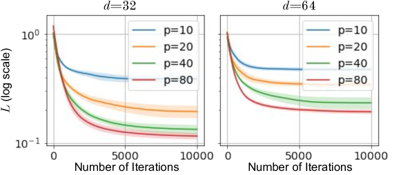
Figure 1: Sublinear convergence of QNN training. For QNNs with Pauli measurements for a classification task, the (log-scaled) training curves flatten as the number of iterations increases, indicating a sublinear convergence. The flattening of training curves remains for increasing numbers of parameters $p=10,20,40,80$. The training curves are averaged over 10 random initialization, and the error bars are the halves of standard deviations.

4 Asymptotic Dynamics of QNNs

As demonstrated in the previous section, the dynamics of the QNN training deviates from the kernel regression for any choices of the number of parameters $p$ and the dimension $d$ in the setting of Pauli measurements for classification. This calls for a new characterization of the QNN dynamics in the regime of over-parameterization. For a concrete definition of over-parameterization, we consider the family of the periodic ansatze in Definition 1, and refer to the limit of $p\rightarrow\infty$ with a fixed generating Hamiltonian $\boldsymbol{\mathbf{H}}$ as the regime of over-parameterization. In this section, we derive the asymptotic dynamics of QNN training when number of parameters $p$ in the periodic ansatze goes to infinity. We start by decomposing the dynamics of the residual ${\boldsymbol{\mathbf{r}}({\boldsymbol{\mathbf{\theta}}(t)})}$ into a term corresponding to the asymptotic dynamics, and a term of perturbation that vanishes as $p\rightarrow\infty$. As mentioned before, in the context of the gradient flow, the choice of $\eta$ is merely a scaling of the time and therefore arbitrary. For a QNN instance with $m$ training samples and a $p$-parameter ansatz generated by a Hermitian $\boldsymbol{\mathbf{H}}$ as defined in Line (2), we choose $\eta$ to be $\frac{m}{p}\frac{d^{2}-1}{\operatorname{tr}(\boldsymbol{\mathbf{H}}^{2})}$ to facilitate the presentation:

Lemma 4.1 (Decomposition of the residual dynamics).

Let $\mathcal{S}$ be a training set with $m$ samples $\{(\boldsymbol{\mathbf{\rho}}_{j},y_{j})\}_{j=1}^{m}$, and let $\boldsymbol{\mathbf{U}}(\boldsymbol{\mathbf{\theta}})$ be a $p$-parameter ansatz generated by a non-zero $\boldsymbol{\mathbf{H}}$ as in Line 2. Consider a QNN instance with a training set $\mathcal{S}$, ansatz $\boldsymbol{\mathbf{U}}(\boldsymbol{\mathbf{\theta}})$ and a measurement ${\boldsymbol{\mathbf{M}}_{0}}$. Under the gradient flow with $\eta=\frac{m}{p}\frac{d^{2}-1}{\operatorname{tr}(\boldsymbol{\mathbf{H}}^{2})}$, the residual vector $\boldsymbol{\mathbf{r}}(t)$ as a function of time $t$ through ${\boldsymbol{\mathbf{\theta}}(t)}$ evolves as

$$\frac{d\boldsymbol{\mathbf{r}}(t)}{dt}=-({\boldsymbol{\mathbf{K}}_{\mathsf{asym}}}(t)+{\boldsymbol{\mathbf{K}}_{\mathsf{pert}}}(t))\boldsymbol{\mathbf{r}}(t)$$ (6)

where both ${\boldsymbol{\mathbf{K}}_{\mathsf{asym}}}$ and ${\boldsymbol{\mathbf{K}}_{\mathsf{pert}}}$ are functions of time through the parameterized measurement ${\boldsymbol{\mathbf{M}}({\boldsymbol{\mathbf{\theta}}(t)})}$, such that

$$({\boldsymbol{\mathbf{K}}_{\mathsf{asym}}}(t))_{ij} :=\operatorname{tr}\big{(}{i}[\boldsymbol{\mathbf{M}}(t),\boldsymbol{\mathbf{\rho}}_{i}]\ {i}[\boldsymbol{\mathbf{M}}(t),\boldsymbol{\mathbf{\rho}}_{j}]\big{)},$$ (7)

$$({\boldsymbol{\mathbf{K}}_{\mathsf{pert}}}(t))_{ij} :=\operatorname{tr}\big{(}{i}[\boldsymbol{\mathbf{M}}(t),\boldsymbol{\mathbf{\rho}}_{i}]\otimes{i}[\boldsymbol{\mathbf{M}}(t),\boldsymbol{\mathbf{\rho}}_{j}]\Delta(t)\big{)}.$$ (8)

Here $\Delta(t)$ is a $d^{2}\times d^{2}$ Hermitian as a function of $t$ through $\boldsymbol{\mathbf{\theta}}(t)$.

Under the random initialization by sampling $\{\boldsymbol{\mathbf{U}}_{l}\}_{l=1}^{p}$ i.i.d. from the haar measure over the special unitary group $SU(d)$, $\Delta(0)$ concentrates at zero as $p$ increases. We further show that $\Delta(t)-\Delta(0)$ has a bounded operator norm decreasing with number of parameters. This allows us to associate the convergence of the over-parameterized QNN with the properties of ${\boldsymbol{\mathbf{K}}_{\mathsf{asym}}}(t)$:

Theorem 4.2 (Linear convergence of QNN with mean-square loss).

Let $\mathcal{S}$ be a training set with $m$ samples $\{(\boldsymbol{\mathbf{\rho}}_{j},y_{j})\}_{j=1}^{m}$, and let $\boldsymbol{\mathbf{U}}(\boldsymbol{\mathbf{\theta}})$ be a $p$-parameter ansatz generated by a non-zero $\boldsymbol{\mathbf{H}}$ as in Line (2). Consider a QNN instance with the training set $\mathcal{S}$, ansatz $\boldsymbol{\mathbf{U}}(\boldsymbol{\mathbf{\theta}})$ and a measurement ${\boldsymbol{\mathbf{M}}_{0}}$, trained by gradient flow with $\eta=\frac{m}{p}\frac{d^{2}-1}{\operatorname{tr}(\boldsymbol{\mathbf{H}}^{2})}$. Then for sufficiently large number of parameters $p$, if the smallest eigenvalue of ${\boldsymbol{\mathbf{K}}_{\mathsf{asym}}}(t)$ is greater than a constant $C_{0}$, then with high probability over the random initialization of the periodic ansatz, the loss function converges to zero at a linear rate

$$L(t)\leq L(0)\exp(-\frac{C_{0}t}{2}).$$ (9)

We defer the proof to Section B.2. Similar to $\boldsymbol{\mathbf{r}}(t)$, the evolution of $\boldsymbol{\mathbf{M}}(t)$ decomposes into an asymptotic term

$$\frac{d}{dt}\boldsymbol{\mathbf{M}}(t)=\sum_{j=1}^{m}r_{j}[\boldsymbol{\mathbf{M}}(t),[\boldsymbol{\mathbf{M}}(t),\boldsymbol{\mathbf{\rho}}_{j}]]$$ (10)

and a perturbative term depending on $\Delta(t)$. Theorem 4.2 allows us to study the behavior of an over-parameterized QNN by simulating/characterizing the asymptotic dynamics of $\boldsymbol{\mathbf{M}}(t)$, which is significantly more accessible.

Application: QNN with one training sample

To demonstrate the proposed asymptotic dynamics as a tool for analyzing over-parameterized QNNs, we study the convergence of the QNN with one training sample $m=1$. To set a separation from the regime of the sublinear convergence, consider the following setting: let ${\boldsymbol{\mathbf{M}}_{0}}$ be a Pauli measurement, for any input state $\boldsymbol{\mathbf{\rho}}$, instead of assigning $\hat{y}=\operatorname{tr}(\boldsymbol{\mathbf{\rho}}\boldsymbol{\mathbf{U}}(\boldsymbol{\mathbf{\theta}})^{\dagger}{\boldsymbol{\mathbf{M}}_{0}}\boldsymbol{\mathbf{U}}(\boldsymbol{\mathbf{\theta}}))$, take $\gamma\operatorname{tr}(\boldsymbol{\mathbf{\rho}}\boldsymbol{\mathbf{U}}(\boldsymbol{\mathbf{\theta}})^{\dagger}{\boldsymbol{\mathbf{M}}_{0}}\boldsymbol{\mathbf{U}}(\boldsymbol{\mathbf{\theta}}))$ as the prediction $\hat{y}$ at $\boldsymbol{\mathbf{\theta}}$ for a scaling factor $\gamma>1.0$. The $\gamma$-scaling of the measurement outcome can be viewed as a classical processing in the context of quantum information, or as an activation function (or a link function) in the context of machine learning, and is equivalent to a QNN with measurement $\gamma{\boldsymbol{\mathbf{M}}_{0}}$. The following corollary implies the convergence of 1-sample QNN for $\gamma>1.0$ under a mild initial condition:

Corollary 4.3.

Let $\boldsymbol{\mathbf{\rho}}$ be a $d$-dimensional pure state, and let $y$ be $\pm 1$. Consider a QNN instance with a Pauli measurement ${\boldsymbol{\mathbf{M}}_{0}}$, an one-sample training set $\mathcal{S}=\{(\boldsymbol{\mathbf{\rho}},y)\}$ and an ansatz $\boldsymbol{\mathbf{U}}(\boldsymbol{\mathbf{\theta}})$ defined in Line (2). Assume the scaling factor $\gamma>1.0$ and $p\rightarrow\infty$ with $\eta=\frac{d^{2}-1}{p\operatorname{tr}(\boldsymbol{\mathbf{H}}^{2})}$. Under the initial condition that the prediction at $t=0$, $\hat{y}(0)$ is less than 1, the objective function converges linearly with

$$L(t)\leq L(0)\exp(-C_{1}t)$$ (11)

with the convergence rate $C_{1}\geq\gamma^{2}-1$.

With a scaling factor $\gamma$ and training set $\{(\boldsymbol{\mathbf{\rho}}_{j},y_{j})\}_{j=1}^{m}$, the objective function, as a function of the parameterized measurement $\boldsymbol{\mathbf{M}}(t)$, reads as: $L(\boldsymbol{\mathbf{M}}(t))=\frac{1}{2m}\sum_{j=1}^{m}(\gamma\operatorname{tr}(\boldsymbol{\mathbf{\rho}}_{j}\boldsymbol{\mathbf{M}}(t))-y_{j})^{2}$. As stated in Theorem 4.2, for sufficiently large number of parameters $p$, the convergence rate of the residual $\boldsymbol{\mathbf{r}}(t)$ is determined by ${\boldsymbol{\mathbf{K}}_{\mathsf{asym}}}(t)$, as the asymptotic dynamics of $\boldsymbol{\mathbf{r}}(t)$ reads as $\frac{d}{dt}\boldsymbol{\mathbf{r}}=-{\boldsymbol{\mathbf{K}}_{\mathsf{asym}}}(\boldsymbol{\mathbf{M}}(t))\boldsymbol{\mathbf{r}}(t)$ with the chosen $\eta$. For $m=1$, the asymptotic matrix ${\boldsymbol{\mathbf{K}}_{\mathsf{asym}}}$ reduces to a scalar $k(t)=-\operatorname{tr}([\gamma\boldsymbol{\mathbf{M}}(t),\boldsymbol{\mathbf{\rho}}]^{2})=2(\gamma^{2}-\hat{y}(t)^{2})$. $\hat{y}(t)$ approaches the label $y$ if $k(t)$ is strictly positive, which is guaranteed for $\hat{y}(t)<\gamma$. Therefore $|\hat{y}(0)|<1$ implies that $|\hat{y}(t)|<1$ and $k(t)\geq 2(\gamma^{2}-1)$ for all $t>0$.

In Figure 2 (top), we plot the training curves of one-sample QNNs with $p=320$ and varying $\gamma=1.2,1.4,2.0,4.0,8.0$ with the same learning rate $\eta=1e-3/p$. As predicted in Corollary 4.3, the rate of convergence increases with the scaling factor $\gamma$. The proof of the corollary additionally implies that $k(t)$ depends on $\hat{y}(t)$: the convergence rate changes over time as the prediction $\hat{y}$ changes. Therefore, despite the linear convergence, the dynamics is different from that of kernel regression, where the kernel remains constant during training in the limit $p\rightarrow\infty$.

In Figure 2 (bottom), we plot the empirical rate of convergence $-\frac{d}{dt}\ln L(t)$ against the rate predicted by $\hat{y}$. Each data point is calculated for QNNs with different $\gamma$ at different time steps by differentiating the logarithms of the training curves. The scatter plot displays an approximately linear dependency, indicating the proposed asymptotic dynamics is capable of predicting how the convergence rate changes during training, which is beyond the explanatory power of the kernel regression model. Note that the slope of the linear relation is not exactly one. This is because we choose a learning rate much smaller than $\eta$ in the corollary statement to simulate the dynamics of gradient flow.

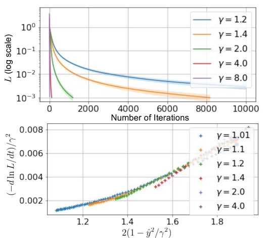
Figure 2: (Top) The training curves of one-sample QNNs with varying $\gamma$. The smallest convergence rate $-d\ln L/dt$ during training (i.e. the slope of the training curves under the log scale) increases with $\gamma$. (Bottom) The convergence rate $-d\ln L/dt|_{t=T}$ as a function of $2(\gamma^{2}-\hat{y}^{2}(T))$ (jointly scaled by $1/\gamma^{2}$ for visualization) are evaluated at different time steps $T$ for different $\gamma$. The approximately linear dependency shows that the proposed dynamics captures the QNN convergence beyond the explanatory power of the kernel regressions.

QNNs with one training sample have been considered before (e.g. Liu et al. (2022a)), where the linear convergence has been shown under the assumption of “frozen QNTK”, namely assuming $\boldsymbol{\mathbf{K}}$, the time derivative of the log residual remains almost constant throughout training. In the corollary above, we provide an end-to-end proof for the one-sample linear convergence without assuming a frozen $\mathbf{K}$. In fact, we observe that in our setting $\mathbf{K}=2(\gamma^{2}-\hat{y}(t))$ changes with $\hat{y}(t)$ (see also Figure 2) and is therefore not frozen.

QNN convergence for $m>1$

To characterize the convergence of QNNs with $m>1$, we seek to empirically study the asymptotic dynamics in Line (10). According to Theorem 4.2, the (linear) rate of convergence is lower-bounded by the smallest eigenvalue of ${\boldsymbol{\mathbf{K}}_{\mathsf{asym}}}(t)$, up to an constant scaling. In Figure 3, we simulate the asymptotic dynamics with various combinations of $(\gamma,d,m)$, and evaluate the smallest eigenvalue of ${\boldsymbol{\mathbf{K}}_{\mathsf{asym}}}(t)$ throughout the dynamics (Figure 3, details deferred to Section D). For sufficiently large dimension $d$, the smallest eigenvalue of ${\boldsymbol{\mathbf{K}}_{\mathsf{asym}}}$ depends on the ratio between the number of samples and the system dimension $m/d$ and is proportional to the square of the scaling factor $\gamma^{2}$.

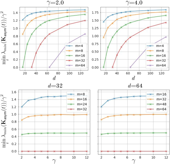
Figure 3: The smallest eigenvalue of ${\boldsymbol{\mathbf{K}}_{\mathsf{asym}}}$ for the asymptotic dynamics with varying system dimension $d$, scaling factor $\gamma$ and number of training samples $m$. For sufficiently large $d$, the smallest eigenvalue depends on the ratio $m/d$ and is proportional to the square of the scaling factor $\gamma^{2}$.

Empirically, we observe that the smallest convergence rates for training QNNs are obtained near the global minima (See Figure 6 in the appendix), suggesting the bottleneck of convergence occurs when $L$ is small.

We now give theoretical evidence that, at most of the global minima, the eigenvalues of ${\boldsymbol{\mathbf{K}}_{\mathsf{asym}}}$ are lower bounded by $2\gamma^{2}(1-1/\gamma^{2}-O(m^{2}/d))$, suggesting a linear convergence in the neighborhood of these minima. To make this notion precise, we define the uniform measure over global minima as follows: consider a set of pure input states $\{\boldsymbol{\mathbf{\rho}}_{j}=\boldsymbol{\mathbf{v}}_{j}\boldsymbol{\mathbf{v}}_{j}^{\dagger}\}_{j=1}^{m}$ that are mutually orthogonal (i.e. $\boldsymbol{\mathbf{v}}_{i}^{\dagger}\boldsymbol{\mathbf{v}}_{j}=0$ if $i\neq j$). For a large dimension $d$, the global minima of the asymptotic dynamics is achieved when the objective function is $0$. Let $\boldsymbol{\mathbf{u}}_{j}(t)$ (resp. $\boldsymbol{\mathbf{w}}_{j}(t)$) denote the components of $\boldsymbol{\mathbf{v}}_{j}$ projected to the positive (resp. negative) subspace of the measurement $\boldsymbol{\mathbf{M}}(t)$ at the global minima. Recall that for a $\gamma$-scaled QNN with a Pauli measurement, the predictions $\hat{y}(t)=\gamma\operatorname{tr}(\rho_{j}\boldsymbol{\mathbf{M}}(t))=\gamma(\boldsymbol{\mathbf{u}}_{j}^{\dagger}(t)\boldsymbol{\mathbf{u}}_{j}(t)-\boldsymbol{\mathbf{w}}_{j}^{\dagger}(t)\boldsymbol{\mathbf{w}}_{j}(t))$. At the global minima, we have $\boldsymbol{\mathbf{u}}_{j}(t)=\frac{1}{2}(1\pm 1/\gamma)\hat{\boldsymbol{\mathbf{u}}}_{j}(t)$ for some unit vector $\hat{\boldsymbol{\mathbf{u}}}_{j}(t)$ for the $j$-th training sample with label $\pm 1$. On the other hand, given a set of unit vectors $\{\hat{\boldsymbol{\mathbf{u}}}_{j}\}_{j=1}^{m}$ in the positive subspace, there is a corresponding set of $\{\boldsymbol{\mathbf{u}}_{j}(t)\}_{j=1}^{m}$ and $\{\boldsymbol{\mathbf{w}}_{j}(t)\}_{j=1}^{m}$ such that $L=0$ for sufficiently large $d$. By uniformly and independently sampling a set of unit vectors $\{\hat{\boldsymbol{\mathbf{u}}}_{j}\}_{j=1}^{m}$ from the $d/2$-dimensional subspace associated with the positive eigenvalues of $\boldsymbol{\mathbf{M}}(t)$, we induce a uniform distribution over all the global minima. The next theorem characterizes ${\boldsymbol{\mathbf{K}}_{\mathsf{asym}}}$ under such an induced uniform distribution over all the global minima:

Theorem 4.4.

Let $\mathcal{S}=\{(\boldsymbol{\mathbf{\rho}}_{j},y_{j})\}_{j=1}^{m}$ be a training set with orthogonal pure states $\{\boldsymbol{\mathbf{\rho}}_{j}\}_{j=1}^{m}$ and equal number of positive and negative labels $y_{j}\in\{\pm 1\}$. Consider the smallest eigenvalue $\lambda_{g}$ of ${\boldsymbol{\mathbf{K}}_{\mathsf{asym}}}$ at the global minima of the asymptotic dynamics of an over-parameterized QNN with the training set $\mathcal{S}$, scaling factor $\gamma$ and system dimension $d$. With probability $\geq 1-\delta$ over the uniform measure over all the global minima

$$\lambda_{g}\geq 2\gamma^{2}(1-\frac{1}{\gamma^{2}}-C_{2}\max\{\frac{m^{2}}{d},\frac{m}{d}\log\frac{2}{\delta}\}),$$ (12)

which is strictly positive for large $\gamma>1$ and $d=\Omega(\mathsf{poly}(m))$. Here $C_{2}$ is a positive constant.

We defer the proof of Theorem 4.4 to Section C in the appendix. A similar notion of a uniform measure over global minima was also used in Canatar et al. (2021). Notice that the uniformness is dependent on the parameterization of the global minima, and the uniform measure over all the global minima is not necessarily the measure induced by random initialization and gradient-based training. Therefore Theorem 4.4 is not a rigorous depiction of the distribution of convergence rate for a randomly-initialized over-parameterized QNN. Yet the prediction of the theorem aligns well with the empirical observations in Figure 3 and suggests that by scaling the QNN measurements, a faster convergence can be achieved: In Figure 4, we simulate $p$-parameter QNNs with dimension $d=32$ and $64$ with a scaling factor $\gamma=4.0$ using the same setup as in Figure 1. The training early stops when the average $L(t)$ over the random seeds is less than $1\times 10^{-2}$. In contrast to Figure 1, the convergence rate $-d\ln L/dt$ does not vanish as $L\rightarrow 0$, suggesting a simple (constant) scaling of the measurement outcome can lead to convergence within much fewer number of iterations.

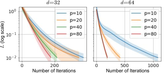
Figure 4: Training curves of QNNs with $\gamma=4.0$ for learning a $4$-sample dataset with labels $\pm 1$. For $p=10,20,40,80$, the rate of convergence is greater than $0$ as $L\rightarrow 0$, and it takes less than $1000$ iterations for $L$ in most of the instances to convergence below $1\times 10^{-2}$. In contrast, in Figure 1, $L>1\times 10^{-1}$ after $10000$ iterations despite the increasing number of parameters.

Another implication of Theorem 4.4 is the deviation of QNN dynamics from any kernel regressions. By straight-forward calculation, the normalized matrix ${\boldsymbol{\mathbf{K}}_{\mathsf{asym}}}(0)/\gamma^{2}$ at the random initialization is independent of the choices of $\gamma$. In contrast, the typical value of $\lambda_{g}/\gamma^{2}$ in Theorem 4.4 is dependent on $\gamma^{2}$, suggesting non-negligible changes in the matrix ${\boldsymbol{\mathbf{K}}_{\mathsf{asym}}}(t)$ governing the dynamics of $\boldsymbol{\mathbf{r}}$ for finite scaling factors $\gamma$. Such phenomenon is empirically verified in Figure 5 in the appendix.

5 Limitations and Outlook

In the setting of $m>1$, the proof of the linear convergence of QNN training (Section 4) relies on the convergence of the asymptotic QNN dynamics as a premise. Given our empirical results, an interesting future direction might be to rigorously characterize the condition for the convergence of the asymptotic dynamics. Also we mainly consider (variants of) two-outcome measurements ${\boldsymbol{\mathbf{M}}_{0}}$ with two eigensubspaces. It might be interesting to look into measurements with more complicated spectrums and see how the shapes of the spectrums affect the rates of convergence.

A QNN for learning a classical dataset is composed of three parts: a classical-to-quantum encoder, a quantum classifier and a readout measurement. Here we have mainly focused on the stage after encoding, i.e. training a QNN classifier to manipulate the density matrices containing classical information that are potentially too costly for a classically-implemented linear model. Our analysis highlights the necessity for measurement design, assuming the design of the quantum classifier mixes to the full $d\times d$ special unitary group. Our result can be combined with existing techniques of classifier designs (i.e. ansatz design) (Ragone et al. (2022); Larocca et al. (2021); Wang et al. (2022); You et al. (2022)) by engineering the invariant subspaces, or be combined with encoder designs explored in (Huang et al., 2021; Du et al., 2022).

Disclaimer

This paper was prepared with synthetic data and for informational purposes by the teams of researchers from the various institutions identified above, including the Global Technology Applied Research Center of JPMorgan Chase & Co. This paper is not a product of the JPMorgan Chase Institute. Neither JPMorgan Chase & Co. nor any of its affiliates make any explicit or implied representation or warranty and none of them accept any liability in connection with this paper, including, but limited to, the completeness, accuracy, reliability of information contained herein and the potential legal, compliance, tax or accounting effects thereof. This document is not intended as investment research or investment advice, or a recommendation, offer or solicitation for the purchase or sale of any security, financial instrument, financial product or service, or to be used in any way for evaluating the merits of participating in any transaction.

Appendix A Proofs for Section 3

A.1 Proof of Lemma 3.1

See 3.1

Proof.

For succinctness, we drop the dependency on ${\boldsymbol{\mathbf{\theta}}(t)}$ when there are no ambiguity. The unitary $\boldsymbol{\mathbf{U}}_{r:p}(\boldsymbol{\mathbf{\theta}})$ depends on $\boldsymbol{\mathbf{\theta}}_{l}$ for $l\geq r$:

$$\frac{\partial\boldsymbol{\mathbf{U}}_{r:p}}{\partial\theta_{l}}=\boldsymbol{\mathbf{U}}_{l:p}(\boldsymbol{\mathbf{\theta}})(-{\mathrm{i}}{\boldsymbol{\mathbf{H}}^{(l)}})\boldsymbol{\mathbf{U}}_{r:l-1}(\boldsymbol{\mathbf{\theta}})=-{\mathrm{i}}\boldsymbol{\mathbf{U}}_{l:p}{\boldsymbol{\mathbf{H}}^{(l)}}\boldsymbol{\mathbf{U}}_{l:p}^{\dagger}\boldsymbol{\mathbf{U}}_{r:p}.$$ (13)

Therefore for all $l\in[p]$

$$\frac{\partial\boldsymbol{\mathbf{M}}(\boldsymbol{\mathbf{\theta}}(t))}{\partial\theta_{l}} =\boldsymbol{\mathbf{U}}_{0}^{\dagger}\left(\frac{\partial\boldsymbol{\mathbf{U}}_{1:p}}{\partial\theta_{l}}\right)^{\dagger}{\boldsymbol{\mathbf{M}}_{0}}\boldsymbol{\mathbf{U}}_{{1:p}}\boldsymbol{\mathbf{U}}_{0}+\boldsymbol{\mathbf{U}}_{0}^{\dagger}\boldsymbol{\mathbf{U}}_{1:p}^{\dagger}{\boldsymbol{\mathbf{M}}_{0}}\frac{\partial\boldsymbol{\mathbf{U}}_{{1:p}}}{\partial\theta_{l}}\boldsymbol{\mathbf{U}}_{0},$$ (14)

$$={\mathrm{i}}(\boldsymbol{\mathbf{U}}_{0}^{\dagger}\boldsymbol{\mathbf{U}}_{1:p}^{\dagger}\boldsymbol{\mathbf{U}}_{l:p}{\boldsymbol{\mathbf{H}}^{(l)}}\boldsymbol{\mathbf{U}}_{l:p}^{\dagger}{\boldsymbol{\mathbf{M}}_{0}}\boldsymbol{\mathbf{U}}_{1:p}\boldsymbol{\mathbf{U}}_{0})-{\mathrm{i}}(\boldsymbol{\mathbf{U}}_{0}^{\dagger}\boldsymbol{\mathbf{U}}_{1:p}^{\dagger}{\boldsymbol{\mathbf{M}}_{0}}\boldsymbol{\mathbf{U}}_{l:p}{\boldsymbol{\mathbf{H}}^{(l)}}\boldsymbol{\mathbf{U}}_{l:p}^{\dagger}\boldsymbol{\mathbf{U}}_{1:p}\boldsymbol{\mathbf{U}}_{0}),$$ (15)

$$={\mathrm{i}}[{\boldsymbol{\mathbf{H}}_{l}},\boldsymbol{\mathbf{M}}(\boldsymbol{\mathbf{\theta}}(t))].$$ (16)

By the chain rule with matrix parameters, we have

$$\frac{\partial L(\boldsymbol{\mathbf{\theta}}(t))}{\partial\theta_{l}}=\operatorname{tr}\big{(}\nabla_{\boldsymbol{\mathbf{M}}}L\frac{\partial\boldsymbol{\mathbf{M}}}{\partial\theta_{l}}\big{)}={\mathrm{i}}\operatorname{tr}(\nabla_{\boldsymbol{\mathbf{M}}}L[{\boldsymbol{\mathbf{H}}_{l}},\boldsymbol{\mathbf{M}}(\boldsymbol{\mathbf{\theta}}(t))]).$$ (17)

Furthermore, due to the gradient flow dynamics,

$$\frac{d{\boldsymbol{\mathbf{M}}(\boldsymbol{\mathbf{\theta}}(t))}}{dt} =\sum_{l=1}^{p}\frac{d\theta_{l}}{dt}\frac{\partial\boldsymbol{\mathbf{M}}(\boldsymbol{\mathbf{\theta}}(t))}{\partial\theta_{l}}=-\eta\sum_{l=1}^{p}\frac{\partial L(\boldsymbol{\mathbf{\theta}}(t))}{\partial\theta_{l}}\frac{\partial\boldsymbol{\mathbf{M}}(\boldsymbol{\mathbf{\theta}}(t))}{\partial\theta_{l}},$$ (18)

$$=\eta\sum_{l=1}^{p}\operatorname{tr}(\nabla_{\boldsymbol{\mathbf{M}}}L[{\boldsymbol{\mathbf{H}}_{l}},\boldsymbol{\mathbf{M}}(\boldsymbol{\mathbf{\theta}}(t))])[{\boldsymbol{\mathbf{H}}_{l}},\boldsymbol{\mathbf{M}}(\boldsymbol{\mathbf{\theta}}(t))].$$ (19)

By plugging in $\nabla_{\boldsymbol{\mathbf{M}}}L=-\frac{1}{m}\sum_{j=1}^{m}r_{j}\boldsymbol{\mathbf{\rho}}_{j}$, we show that the parameterized measurement $\boldsymbol{\mathbf{M}}(\boldsymbol{\mathbf{\theta}})=\boldsymbol{\mathbf{U}}^{\dagger}(\boldsymbol{\mathbf{\theta}}){\boldsymbol{\mathbf{M}}_{0}}\boldsymbol{\mathbf{U}}(\boldsymbol{\mathbf{\theta}})$ follows the dynamics

$$d\boldsymbol{\mathbf{M}}(\boldsymbol{\mathbf{\theta}}(t))/dt=\frac{\eta}{m}\sum_{l=1}^{p}\operatorname{tr}\big{(}\sum_{j=1}^{m}r_{j}\boldsymbol{\mathbf{\rho}}_{j}{\mathrm{i}}[{\boldsymbol{\mathbf{H}}_{l}},\boldsymbol{\mathbf{M}}(\boldsymbol{\mathbf{\theta}}(t))]\big{)}{\mathrm{i}}[{\boldsymbol{\mathbf{H}}_{l}},\boldsymbol{\mathbf{M}}(\boldsymbol{\mathbf{\theta}}(t))].$$ (20)

By definition $r_{i}:=y_{i}-\hat{y}_{i}$, and

$$\frac{dr_{i}}{dt} =-\frac{d\operatorname{tr}(\boldsymbol{\mathbf{\rho}}_{i}\boldsymbol{\mathbf{M}}(\boldsymbol{\mathbf{\theta}}(t)))}{dt}=-\operatorname{tr}\big{(}\boldsymbol{\mathbf{\rho}}_{i}\frac{d{\boldsymbol{\mathbf{M}}(\boldsymbol{\mathbf{\theta}}(t))}}{dt}\big{)}$$ (21)

$$=-\frac{\eta}{m}\sum_{l=1}^{p}\operatorname{tr}\big{(}\sum_{j=1}^{m}r_{j}\boldsymbol{\mathbf{\rho}}_{j}{\mathrm{i}}[{\boldsymbol{\mathbf{H}}_{l}},\boldsymbol{\mathbf{M}}(\boldsymbol{\mathbf{\theta}}(t))]\big{)}\operatorname{tr}\big{(}\boldsymbol{\mathbf{\rho_{i}}}{\mathrm{i}}[{\boldsymbol{\mathbf{H}}_{l}},\boldsymbol{\mathbf{M}}(\boldsymbol{\mathbf{\theta}}(t))]\big{)}$$ (22)

$$=-\frac{\eta}{m}\sum_{j=1}^{m}r_{j}\big{(}\operatorname{tr}\big{(}\boldsymbol{\mathbf{\rho}}_{i}{\mathrm{i}}[{\boldsymbol{\mathbf{H}}_{l}},\boldsymbol{\mathbf{M}}(\boldsymbol{\mathbf{\theta}}(t))]\big{)}\operatorname{tr}\big{(}\boldsymbol{\mathbf{\rho}}_{j}{\mathrm{i}}[{\boldsymbol{\mathbf{H}}_{l}},\boldsymbol{\mathbf{M}}(\boldsymbol{\mathbf{\theta}}(t))]\big{)}\big{)}$$ (23)

$$=-\frac{\eta}{m}\sum_{j=1}^{m}r_{j}\big{(}\operatorname{tr}\big{(}{\mathrm{i}}[{\boldsymbol{\mathbf{M}}(\boldsymbol{\mathbf{\theta}}(t))},\boldsymbol{\mathbf{\rho}}_{i}]{\boldsymbol{\mathbf{H}}_{l}}\big{)}\operatorname{tr}\big{(}{\mathrm{i}}[{\boldsymbol{\mathbf{M}}(\boldsymbol{\mathbf{\theta}}(t))},\boldsymbol{\mathbf{\rho}}_{j}]{\boldsymbol{\mathbf{H}}_{l}}\big{)}\big{)}.$$ (24)

The last equality is due to the cyclicity of the trace operation. Making the identification $K_{ij}({\boldsymbol{\mathbf{M}}(\boldsymbol{\mathbf{\theta}}(t))})=\big{(}\operatorname{tr}\big{(}{\mathrm{i}}[{\boldsymbol{\mathbf{M}}(\boldsymbol{\mathbf{\theta}}(t))},\boldsymbol{\mathbf{\rho}}_{i}]{\boldsymbol{\mathbf{H}}_{l}}\big{)}\operatorname{tr}\big{(}{\mathrm{i}}[{\boldsymbol{\mathbf{M}}(\boldsymbol{\mathbf{\theta}}(t))},\boldsymbol{\mathbf{\rho}}_{j}]{\boldsymbol{\mathbf{H}}_{l}}\big{)}\big{)}$, we have

$$\frac{d{\boldsymbol{\mathbf{r}}({\boldsymbol{\mathbf{\theta}}(t)})}}{dt}=-\frac{\eta}{m}\boldsymbol{\mathbf{K}}({\boldsymbol{\mathbf{M}}({\boldsymbol{\mathbf{\theta}}(t)})}){\boldsymbol{\mathbf{r}}({\boldsymbol{\mathbf{\theta}}(t)})}.$$ (25)

∎

A.2 Proof of Theorem 3.2

Proof.

The mean squared loss function $L({\boldsymbol{\mathbf{\theta}}(t)})$ can be expressed as $\frac{1}{2m}\boldsymbol{\mathbf{r}}({\boldsymbol{\mathbf{\theta}}(t)})^{T}\boldsymbol{\mathbf{r}}({\boldsymbol{\mathbf{\theta}}(t)})$. Using Lemma 3.1, the rate of convergence can be lower-bounded as

$$\frac{1}{{L({\boldsymbol{\mathbf{\theta}}(t)})}}\frac{d{L({\boldsymbol{\mathbf{\theta}}(t)})}}{dt}$$ (26)

$$= \frac{1}{{\boldsymbol{\mathbf{r}}({\boldsymbol{\mathbf{\theta}}(t)})}^{T}{\boldsymbol{\mathbf{r}}({\boldsymbol{\mathbf{\theta}}(t)})}}\frac{d}{dt}{\boldsymbol{\mathbf{r}}({\boldsymbol{\mathbf{\theta}}(t)})}^{T}{\boldsymbol{\mathbf{r}}({\boldsymbol{\mathbf{\theta}}(t)})},$$ (27)

$$= -\frac{2\eta}{m}\cdot\frac{{\boldsymbol{\mathbf{r}}({\boldsymbol{\mathbf{\theta}}(t)})}^{T}\boldsymbol{\mathbf{K}}({\boldsymbol{\mathbf{\theta}}(t)}){\boldsymbol{\mathbf{r}}({\boldsymbol{\mathbf{\theta}}(t)})}}{{\boldsymbol{\mathbf{r}}({\boldsymbol{\mathbf{\theta}}(t)})}^{T}{\boldsymbol{\mathbf{r}}({\boldsymbol{\mathbf{\theta}}(t)})}},$$ (28)

$$\geq -\frac{2\eta}{m}\lambda_{\max}(\boldsymbol{\mathbf{K}}({\boldsymbol{\mathbf{\theta}}(t)})).$$ (29)

The positive semi-definiteness of ${\boldsymbol{\mathbf{K}}({\boldsymbol{\mathbf{\theta}}(t)})}$ suggests that $\lambda_{\max}({\boldsymbol{\mathbf{K}}({\boldsymbol{\mathbf{\theta}}(t)})})\leq\operatorname{tr}({\boldsymbol{\mathbf{K}}({\boldsymbol{\mathbf{\theta}}(t)})})$. We now proceed to bound $\operatorname{tr}({\boldsymbol{\mathbf{K}}({\boldsymbol{\mathbf{\theta}}(t)})})$. Since the eigenvalues of ${\boldsymbol{\mathbf{M}}_{0}}$ and $\boldsymbol{\mathbf{M}}(\boldsymbol{\mathbf{\theta}})$ all lie in $\{\pm 1\}$, $\boldsymbol{\mathbf{M}}({\boldsymbol{\mathbf{\theta}}(t)})$ decomposes into the difference of to projections, $\boldsymbol{\mathbf{\Pi}}_{+}({\boldsymbol{\mathbf{\theta}}(t)})$ and $\boldsymbol{\mathbf{\Pi}}_{-}({\boldsymbol{\mathbf{\theta}}(t)})$, projecting onto the subspaces associated with eigenvalues of $+1$ and $-1$ respectively. When $\hat{y}_{j}$ approaches $y_{j}$, the input state $\boldsymbol{\mathbf{\rho}}_{j}$ lies almost completely in one of the eigen-subspaces, leading to a vanishing commutator ${\mathrm{i}}[{\boldsymbol{\mathbf{M}}({\boldsymbol{\mathbf{\theta}}(t)})},\boldsymbol{\mathbf{\rho}}_{j}]$ such that $K_{jj}({\boldsymbol{\mathbf{\theta}}(t)})$ approaches zero:

Let $\boldsymbol{\mathbf{v}}_{j}$ be the statevector representation of the pure state $\boldsymbol{\mathbf{\rho}}_{j}$, such that $\boldsymbol{\mathbf{\rho}}_{j}=\boldsymbol{\mathbf{v}}_{j}\boldsymbol{\mathbf{v}}_{j}^{\dagger}$. Vector $\boldsymbol{\mathbf{v}}_{j}$ decomposes into the components within the positive and negative eigen-subspaces of ${\boldsymbol{\mathbf{M}}({\boldsymbol{\mathbf{\theta}}(t)})}$: $\boldsymbol{\mathbf{v}}_{j}=\boldsymbol{\mathbf{u}}_{j}({\boldsymbol{\mathbf{\theta}}(t)})+\boldsymbol{\mathbf{w}}_{j}({\boldsymbol{\mathbf{\theta}}(t)})$, where $\boldsymbol{\mathbf{u}}_{j}({\boldsymbol{\mathbf{\theta}}(t)})=\boldsymbol{\mathbf{\Pi}}_{+}({\boldsymbol{\mathbf{\theta}}(t)})\boldsymbol{\mathbf{v}}_{j}$ and $\boldsymbol{\mathbf{w}}_{j}({\boldsymbol{\mathbf{\theta}}(t)})=\boldsymbol{\mathbf{\Pi}}_{-}({\boldsymbol{\mathbf{\theta}}(t)})\boldsymbol{\mathbf{v}}_{j}$. In the following we omit the arguments ${\boldsymbol{\mathbf{\theta}}(t)}$ in $\boldsymbol{\mathbf{u}}_{j}$ and $\boldsymbol{\mathbf{v}}_{j}$ for succinctness, but the time dependence is to be implicitly understood. The commutator between the parameterized measurement and the input state can be written as $[{\boldsymbol{\mathbf{M}}({\boldsymbol{\mathbf{\theta}}(t)})},\boldsymbol{\mathbf{\rho}}_{j}]=2(\boldsymbol{\mathbf{u}}_{j}\boldsymbol{\mathbf{w}}_{j}^{\dagger}-\boldsymbol{\mathbf{w}}_{j}\boldsymbol{\mathbf{u}}_{j}^{\dagger})$. Therefore

$$|\operatorname{tr}({\mathrm{i}}[\boldsymbol{\mathbf{M}},\boldsymbol{\mathbf{\rho}}_{j}]{\boldsymbol{\mathbf{H}}_{l}})|\leq 4\left\lVert\mspace{1.0mu}{\boldsymbol{\mathbf{H}}_{l}}\mspace{1.0mu}\right\rVert_{\mathsf{op}}\left\lVert\mspace{1.0mu}\boldsymbol{\mathbf{u}}_{j}\mspace{1.0mu}\right\rVert\left\lVert\mspace{1.0mu}\boldsymbol{\mathbf{w}}_{j}\mspace{1.0mu}\right\rVert.$$ (30)

Assume without loss of generality that the $j$-th label $y_{j}$ is $+1$. Then $\left\lVert\mspace{1.0mu}\boldsymbol{\mathbf{u}}_{j}\mspace{1.0mu}\right\rVert^{2}+\left\lVert\mspace{1.0mu}\boldsymbol{\mathbf{w}}_{j}\mspace{1.0mu}\right\rVert^{2}=\left\lVert\mspace{1.0mu}\boldsymbol{\mathbf{v}}_{j}\mspace{1.0mu}\right\rVert^{2}=1$ by definition, and $\left\lVert\mspace{1.0mu}\boldsymbol{\mathbf{u}}_{j}\mspace{1.0mu}\right\rVert^{2}-\left\lVert\mspace{1.0mu}\boldsymbol{\mathbf{w}}_{j}\mspace{1.0mu}\right\rVert^{2}=\operatorname{tr}({\boldsymbol{\mathbf{M}}({\boldsymbol{\mathbf{\theta}}(t)})}\boldsymbol{\mathbf{\rho}}_{j})=y_{j}-r_{j}=1-r_{j}$. Then $\left\lVert\mspace{1.0mu}\boldsymbol{\mathbf{w}}_{j}\mspace{1.0mu}\right\rVert^{2}=|r_{j}|/2$, and $\left\lVert\mspace{1.0mu}\boldsymbol{\mathbf{u}}_{j}\mspace{1.0mu}\right\rVert^{2}\left\lVert\mspace{1.0mu}\boldsymbol{\mathbf{w}}_{j}\mspace{1.0mu}\right\rVert^{2}=(1-|r_{j}|/2)|r_{j}|/2$.

Therefore we have,

$$K_{jj}(\boldsymbol{\mathbf{\theta}}(t))= \sum_{l=1}^{p}\operatorname{tr}^{2}({\mathrm{i}}[{\boldsymbol{\mathbf{M}}({\boldsymbol{\mathbf{\theta}}(t)})},\boldsymbol{\mathbf{\rho}}_{j}]\boldsymbol{\mathbf{H}}_{l})$$ (31)

$$\leq 16\sum_{l=1}^{p}\left\lVert\mspace{1.0mu}\boldsymbol{\mathbf{H}}_{l}\mspace{1.0mu}\right\rVert_{\mathsf{op}}^{2}\frac{|r_{j}|}{2}(1-\frac{|r_{j}|}{2})$$ (32)

$$\leq 16\sum_{l=1}^{p}\left\lVert\mspace{1.0mu}\boldsymbol{\mathbf{H}}_{l}\mspace{1.0mu}\right\rVert_{\mathsf{op}}^{2}\frac{|r_{j}|}{2}$$ (33)

As a result

$$\frac{1}{L({\boldsymbol{\mathbf{\theta}}(t)})}\frac{d{L({\boldsymbol{\mathbf{\theta}}(t)})}}{dt}$$ (34)

$$\geq-\frac{2\eta}{m}\operatorname{tr}(\boldsymbol{\mathbf{K}}({\boldsymbol{\mathbf{\theta}}(t)}))\geq-\frac{2\eta}{m}\sum_{i=1}^{m}K_{ii}$$ (35)

$$\geq-\frac{16\eta}{m}\sum_{l=1}^{p}\left\lVert\mspace{1.0mu}\boldsymbol{\mathbf{H}}_{l}\mspace{1.0mu}\right\rVert_{\mathsf{op}}^{2}\sum_{i=1}^{m}|r_{j}|$$ (36)

$$\geq-16\sqrt{2}\eta\sum_{l=1}^{p}\left\lVert\mspace{1.0mu}\boldsymbol{\mathbf{H}}_{l}\mspace{1.0mu}\right\rVert_{\mathsf{op}}^{2}\sqrt{L({\boldsymbol{\mathbf{\theta}}(t)})}$$ (37)

$$=-16\sqrt{2}\eta\sum_{l=1}^{p}\left\lVert\mspace{1.0mu}{\boldsymbol{\mathbf{H}}^{(l)}}\mspace{1.0mu}\right\rVert_{\mathsf{op}}^{2}\sqrt{L({\boldsymbol{\mathbf{\theta}}(t)})}.$$ (38)

Here we use the fact that $\sum_{j=1}^{m}|r_{j}|\leq\sqrt{m}\sqrt{{\boldsymbol{\mathbf{r}}({\boldsymbol{\mathbf{\theta}}(t)})}^{T}{\boldsymbol{\mathbf{r}}({\boldsymbol{\mathbf{\theta}}(t)})}}=\sqrt{2m^{2}{L({\boldsymbol{\mathbf{\theta}}(t)})}}$.

The theorem statement follows directly by integrating the inequality above:

$${L({\boldsymbol{\mathbf{\theta}}(t)})}^{-\frac{3}{2}}d{L({\boldsymbol{\mathbf{\theta}}(t)})}\geq-24\eta\sum_{l=1}^{p}\left\lVert\mspace{1.0mu}{\boldsymbol{\mathbf{H}}^{(l)}}\mspace{1.0mu}\right\rVert_{\mathsf{op}}^{2}dt$$ (39)

$$\implies -2d({L({\boldsymbol{\mathbf{\theta}}(t)})}^{-1/2})\geq-24\eta\sum_{l=1}^{p}\left\lVert\mspace{1.0mu}{\boldsymbol{\mathbf{H}}^{(l)}}\mspace{1.0mu}\right\rVert_{\mathsf{op}}^{2}dt$$ (40)

$$\implies L(\boldsymbol{\mathbf{\theta}}(T))^{-\frac{1}{2}}-L(\boldsymbol{\mathbf{\theta}}(0))^{-\frac{1}{2}}\leq 12\eta\sum_{l=1}^{p}\left\lVert\mspace{1.0mu}{\boldsymbol{\mathbf{H}}^{(l)}}\mspace{1.0mu}\right\rVert_{\mathsf{op}}^{2}T$$ (41)

$$\implies L(\boldsymbol{\mathbf{\theta}}(T))^{-\frac{1}{2}}-c_{0}\leq c_{1}T$$ (42)

∎

Note that the same “at most sublinear convergence” holds for a measurement $\mathbf{M}_{0}$ such that $\mathbf{M}_{0}=\boldsymbol{\Pi}_{+}-\boldsymbol{\Pi}_{-}$ and $\boldsymbol{\Pi}_{+}+\boldsymbol{\Pi}_{-}+\boldsymbol{\Pi}_{0}=\mathbf{I}$ for some non-zero projection $\boldsymbol{\Pi}_{0}$. The proof still holds with the following modification: define $s_{j}:=\|\mathbf{u}_{j}\|^{2}+\|\mathbf{w}_{j}\|^{2}\leq 1$, we have

$$\|\mathbf{u}_{j}\|^{2}\cdot\|\mathbf{w}_{j}\|^{2}$$

$$= (\frac{s_{j}-y_{j}+r_{j}}{2})(\frac{s_{j}+y_{j}-r_{j}}{2})$$

$$= \frac{s_{j}^{2}-(y_{j}-r_{j})^{2}}{4}$$

$$\leq \frac{1-(y_{j}-r_{j})^{2}}{4}$$

$$= \frac{(1-y_{j})^{2}+2y_{j}r_{j}-r^{2}_{j}}{4}$$

$$= \frac{y_{j}r_{j}}{2}-\frac{r^{2}_{j}}{4}\leq\frac{y_{j}r_{j}}{2}$$

$$= \frac{|r_{j}|}{2}$$

The last equality follows from the fact that $r_{j}\geq 0$ (resp. $r_{j}\leq 0$) for $y_{j}=1$ (resp. $y_{j}=-1$).

Appendix B Proofs for the asymptotic dynamics

B.1 Proof of Lemma 4.1

See 4.1 Throughout the proof, we make use of the following notations. Let $\mathcal{H}$ be a $d$-dimensional Hilbert space, and let $\{\boldsymbol{\mathbf{e}}_{a}\}_{a\in[d]}$ be a basis of $\mathcal{H}$. We use $\boldsymbol{\mathbf{I}}_{d\times d}$ denote the identity matrix $\sum_{a\in[d]}\boldsymbol{\mathbf{e}}_{a}\boldsymbol{\mathbf{e}}_{a}^{\dagger}$. We use $\otimes$ for kronecker products on vectors, matrices and Hilbert spaces. For the $d^{2}\times d^{2}$-dimensional product space $\mathcal{H}\otimes\mathcal{H}$, let $\boldsymbol{\mathbf{W}}_{d^{2}\times d^{2}}$ denote the swap matrix $\sum_{a,b\in[d]}\boldsymbol{\mathbf{e}}_{a}\boldsymbol{\mathbf{e}}_{b}^{\dagger}\otimes\boldsymbol{\mathbf{e}}_{b}\boldsymbol{\mathbf{e}}_{a}^{\dagger}$.

We will also make use of the well-known integration formula with respect to the haar measure over $d$-dimensional unitaries (see e.g. Collins and Śniady [2006] for more details).

Proof.

As proven in Lemma 3.1, we track the dynamics of the parameterized measurement $\boldsymbol{\mathbf{M}}(\boldsymbol{\mathbf{\theta}})$:

$$\frac{d\boldsymbol{\mathbf{M}}(\boldsymbol{\mathbf{\theta}})}{dt}= \sum_{l=1}^{p}\frac{d\theta_{l}}{dt}\cdot\frac{\partial\boldsymbol{\mathbf{M}}(\boldsymbol{\mathbf{\theta}})}{\partial\theta_{l}}$$ (43)

$$= \sum_{l=1}^{p}(-\eta)\operatorname{tr}\big{(}{i}[\boldsymbol{\mathbf{H}}_{l},\boldsymbol{\mathbf{M}}(\boldsymbol{\mathbf{\theta}})]\nabla_{\boldsymbol{\mathbf{M}}}L\big{)}{i}[\boldsymbol{\mathbf{H}}_{l},\boldsymbol{\mathbf{M}}(\boldsymbol{\mathbf{\theta}})]$$ (44)

$$= \sum_{l=1}^{p}\eta\operatorname{tr}\big{(}{i}[\nabla_{\boldsymbol{\mathbf{M}}}L,\boldsymbol{\mathbf{M}}(\boldsymbol{\mathbf{\theta}})]\boldsymbol{\mathbf{H}}_{l}\big{)}{i}[\boldsymbol{\mathbf{H}}_{l},\boldsymbol{\mathbf{M}}(\boldsymbol{\mathbf{\theta}})]$$ (45)

$$= \sum_{l=1}^{p}\eta{i}[\operatorname{tr}\big{(}{i}[\nabla_{\boldsymbol{\mathbf{M}}}L,\boldsymbol{\mathbf{M}}(\boldsymbol{\mathbf{\theta}})]\boldsymbol{\mathbf{H}}_{l}\big{)}\boldsymbol{\mathbf{H}}_{l},\boldsymbol{\mathbf{M}}(\boldsymbol{\mathbf{\theta}})]$$ (46)

$$= \sum_{l=1}^{p}\eta{i}[\operatorname{tr}_{1}\big{(}({i}[\nabla_{\boldsymbol{\mathbf{M}}}L,\boldsymbol{\mathbf{M}}(\boldsymbol{\mathbf{\theta}})]\otimes\boldsymbol{\mathbf{I}})(\boldsymbol{\mathbf{H}}_{l}\otimes\boldsymbol{\mathbf{H}}_{l})\big{)},\boldsymbol{\mathbf{M}}(\boldsymbol{\mathbf{\theta}})].$$ (47)

Here $\operatorname{tr}_{{1}}(\cdot)$ is the partial trace: Given the product of two Hilbert spaces $\mathcal{H}_{1}\otimes\mathcal{H}_{2}$, the partial trace on the first Hilbert space is a linear mapping such that

$$\operatorname{tr}_{1}\big{(}\mathbf{A}\otimes\mathbf{B}\big{)}=\operatorname{tr}(\mathbf{A})\mathbf{B}$$

for any Hermitians $\mathbf{A}$ and $\mathbf{B}$ on the spaces $\mathcal{H}_{1}$ and $\mathcal{H}_{2}$. By linearity,

$$\operatorname{tr}_{1}\big{(}\sum_{l}\mathbf{A}_{l}\otimes\mathbf{B}_{l}\big{)}=\sum_{l}\operatorname{tr}(\mathbf{A}_{l})\mathbf{B}_{l}$$

for any Hermitians $\{\mathbf{A}_{l}\}$ and $\{\mathbf{B}_{l}\}$ on the spaces $\mathcal{H}_{1}$ and $\mathcal{H}_{2}$.

Let $Z(\boldsymbol{\mathbf{H}},d)$ denote the ratio $\frac{\operatorname{tr}(\boldsymbol{\mathbf{H}}^{2})}{d^{2}-1}$, the learning rate $\eta$ can be expressed as $\frac{m}{pZ(\boldsymbol{\mathbf{H}},d)}$. Let $\boldsymbol{\mathbf{Y}}(\boldsymbol{\mathbf{\theta}}(t))$ denote the normalized $d^{2}\times d^{2}$-complex matrix $\frac{1}{pZ(\boldsymbol{\mathbf{H}},d)}\sum_{l=1}^{p}\boldsymbol{\mathbf{H}}_{l}\otimes\boldsymbol{\mathbf{H}}_{l}$ for $\boldsymbol{\mathbf{H}}_{l}$ defined in Lemma 3.1 and let $\boldsymbol{\mathbf{Y}}^{\star}$ denote $\boldsymbol{\mathbf{W}}_{d^{2}\times d^{2}}-\frac{1}{d}\boldsymbol{\mathbf{I}}_{d^{2}\times d^{2}}$, the asymptotic version of $\boldsymbol{\mathbf{Y}}$. We can accordingly decompose the dynamics into the asymptotic dynamics and the deviation (perturbation) from the asymptotic dynamics:

$$\frac{d\boldsymbol{\mathbf{M}}(\boldsymbol{\mathbf{\theta}})}{dt}= (\eta pZ(\boldsymbol{\mathbf{H}},d)){i}[\operatorname{tr}_{1}\big{(}({i}[\nabla_{\boldsymbol{\mathbf{M}}}L,\boldsymbol{\mathbf{M}}(\boldsymbol{\mathbf{\theta}})]\otimes\boldsymbol{\mathbf{I}})\boldsymbol{\mathbf{Y}}\big{)},\boldsymbol{\mathbf{M}}(\boldsymbol{\mathbf{\theta}})]$$ (48)

$$= (\eta pZ(\boldsymbol{\mathbf{H}},d)){i}[\operatorname{tr}_{1}\big{(}({i}[\nabla_{\boldsymbol{\mathbf{M}}}L,\boldsymbol{\mathbf{M}}(\boldsymbol{\mathbf{\theta}})]\otimes\boldsymbol{\mathbf{I}})\boldsymbol{\mathbf{Y}}^{\star}\big{)},\boldsymbol{\mathbf{M}}(\boldsymbol{\mathbf{\theta}})]$$ (49)

$$+(\eta pZ(\boldsymbol{\mathbf{H}},d)){i}[\operatorname{tr}_{1}\big{(}({i}[\nabla_{\boldsymbol{\mathbf{M}}}L,\boldsymbol{\mathbf{M}}(\boldsymbol{\mathbf{\theta}})]\otimes\boldsymbol{\mathbf{I}})(\boldsymbol{\mathbf{Y}}(\boldsymbol{\mathbf{\theta}}(t))-\boldsymbol{\mathbf{Y}}^{\star})\big{)},\boldsymbol{\mathbf{M}}(\boldsymbol{\mathbf{\theta}})]$$ (50)

$$= (\eta pZ(\boldsymbol{\mathbf{H}},d)){i}[({i}[\nabla_{\boldsymbol{\mathbf{M}}}L,\boldsymbol{\mathbf{M}}(\boldsymbol{\mathbf{\theta}})],\boldsymbol{\mathbf{M}}(\boldsymbol{\mathbf{\theta}})]$$ (51)

$$+(\eta pZ(\boldsymbol{\mathbf{H}},d)){i}[\operatorname{tr}_{1}\big{(}({i}[\nabla_{\boldsymbol{\mathbf{M}}}L,\boldsymbol{\mathbf{M}}(\boldsymbol{\mathbf{\theta}})]\otimes\boldsymbol{\mathbf{I}})(\boldsymbol{\mathbf{Y}}(\boldsymbol{\mathbf{\theta}}(t))-\boldsymbol{\mathbf{Y}}^{\star})\big{)},\boldsymbol{\mathbf{M}}(\boldsymbol{\mathbf{\theta}})]$$ (52)

$$= -(\eta pZ(\boldsymbol{\mathbf{H}},d))[\boldsymbol{\mathbf{M}}(\boldsymbol{\mathbf{\theta}}),[\boldsymbol{\mathbf{M}}(\boldsymbol{\mathbf{\theta}}),\nabla_{\boldsymbol{\mathbf{M}}}L]]$$ (53)

$$-(\eta pZ(\boldsymbol{\mathbf{H}},d))[\boldsymbol{\mathbf{M}}(\boldsymbol{\mathbf{\theta}}),\operatorname{tr}_{1}\big{(}([\boldsymbol{\mathbf{M}}(\boldsymbol{\mathbf{\theta}}),\nabla_{\boldsymbol{\mathbf{M}}}L]\otimes\boldsymbol{\mathbf{I}})(\boldsymbol{\mathbf{Y}}(\boldsymbol{\mathbf{\theta}}(t))-\boldsymbol{\mathbf{Y}}^{\star})\big{)}]$$ (54)

Plugging in that $\nabla_{\boldsymbol{\mathbf{M}}}L(\boldsymbol{\mathbf{M}}(\boldsymbol{\mathbf{\theta}}))=-\frac{1}{m}\sum_{i=1}^{m}r_{i}\boldsymbol{\mathbf{\rho}}_{i}$ with the residual $r_{i}:=y_{i}-\hat{y}_{i}=\operatorname{tr}(\boldsymbol{\mathbf{M}}(\boldsymbol{\mathbf{\theta}})\rho_{i})-y_{i}$:

$$\frac{d\boldsymbol{\mathbf{M}}(\boldsymbol{\mathbf{\theta}})}{dt}= \sum_{j=1}^{m}r_{j}[\boldsymbol{\mathbf{M}}(\boldsymbol{\mathbf{\theta}}),[\boldsymbol{\mathbf{M}}(\boldsymbol{\mathbf{\theta}}),\boldsymbol{\mathbf{\rho}}_{j}]]$$ (55)

$$+ \sum_{j=1}^{m}r_{j}[\boldsymbol{\mathbf{M}}(\boldsymbol{\mathbf{\theta}}),\operatorname{tr}_{1}\big{(}([\boldsymbol{\mathbf{M}}(\boldsymbol{\mathbf{\theta}}),\boldsymbol{\mathbf{\rho}}_{j}]\otimes\boldsymbol{\mathbf{I}})(\boldsymbol{\mathbf{Y}}(\boldsymbol{\mathbf{\theta}}(t))-\boldsymbol{\mathbf{Y}}^{\star})\big{)}]$$ (56)

Trace after multiplying $\boldsymbol{\mathbf{\rho}}_{i}$ on both sides:

$$\frac{dr_{i}}{dt}=-\operatorname{tr}(\boldsymbol{\mathbf{\rho}}_{i}\frac{d\boldsymbol{\mathbf{M}}(\boldsymbol{\mathbf{\theta}})}{dt})= -\sum_{j=1}^{m}r_{j}\operatorname{tr}\big{(}\boldsymbol{\mathbf{\rho}}_{i}[\boldsymbol{\mathbf{M}}(\boldsymbol{\mathbf{\theta}}),[\boldsymbol{\mathbf{M}}(\boldsymbol{\mathbf{\theta}}),\boldsymbol{\mathbf{\rho}}_{j}]]\big{)}$$ (57)

$$-\sum_{j=1}^{m}r_{j}\operatorname{tr}\big{(}\boldsymbol{\mathbf{\rho}}_{i}[\boldsymbol{\mathbf{M}}(\boldsymbol{\mathbf{\theta}}),\operatorname{tr}_{1}\big{(}([\boldsymbol{\mathbf{M}}(\boldsymbol{\mathbf{\theta}}),\boldsymbol{\mathbf{\rho}}_{j}]\otimes\boldsymbol{\mathbf{I}})(\boldsymbol{\mathbf{Y}}(\boldsymbol{\mathbf{\theta}}(t))-\boldsymbol{\mathbf{Y}}^{\star})\big{)}]\big{)}$$ (58)

The lemma follows directly from rearranging: for the first term,

$$-\sum_{j=1}^{m}r_{j}\operatorname{tr}(\boldsymbol{\mathbf{\rho}}_{i}[\boldsymbol{\mathbf{M}}(\boldsymbol{\mathbf{\theta}}),[\boldsymbol{\mathbf{M}}(\boldsymbol{\mathbf{\theta}}),\boldsymbol{\mathbf{\rho}}_{j}]])$$ (59)

$$= -\sum_{j=1}^{m}r_{j}\operatorname{tr}([\boldsymbol{\mathbf{\rho}}_{i},\boldsymbol{\mathbf{M}}(\boldsymbol{\mathbf{\theta}})][\boldsymbol{\mathbf{M}}(\boldsymbol{\mathbf{\theta}}),\boldsymbol{\mathbf{\rho}}_{j}])$$ (60)

$$= -\sum_{j=1}^{m}r_{j}\operatorname{tr}({i}[\boldsymbol{\mathbf{M}}(\boldsymbol{\mathbf{\theta}}),\boldsymbol{\mathbf{\rho}}_{i}]{i}[\boldsymbol{\mathbf{M}}(\boldsymbol{\mathbf{\theta}}),\boldsymbol{\mathbf{\rho}}_{j}]).$$ (61)

For the second term,

$$-\sum_{j=1}^{m}r_{j}\operatorname{tr}\big{(}\boldsymbol{\mathbf{\rho}}_{i}[\boldsymbol{\mathbf{M}}(\boldsymbol{\mathbf{\theta}}),\operatorname{tr}_{1}\big{(}([\boldsymbol{\mathbf{M}}(\boldsymbol{\mathbf{\theta}}),\boldsymbol{\mathbf{\rho}}_{j}]\otimes\boldsymbol{\mathbf{I}})(\boldsymbol{\mathbf{Y}}(\boldsymbol{\mathbf{\theta}}(t))-\boldsymbol{\mathbf{Y}}^{\star})\big{)}]\big{)}$$ (62)

$$= -\sum_{j=1}^{m}r_{j}\operatorname{tr}\big{(}{i}[\boldsymbol{\mathbf{M}}(\boldsymbol{\mathbf{\theta}}),\boldsymbol{\mathbf{\rho}}_{i}]\operatorname{tr}_{1}\big{(}({i}[\boldsymbol{\mathbf{M}}(\boldsymbol{\mathbf{\theta}}),\boldsymbol{\mathbf{\rho}}_{j}]\otimes\boldsymbol{\mathbf{I}})(\boldsymbol{\mathbf{Y}}(\boldsymbol{\mathbf{\theta}}(t))-\boldsymbol{\mathbf{Y}}^{\star})\big{)}\big{)}$$ (63)

$$= -\sum_{j=1}^{m}r_{j}\operatorname{tr}\big{(}(\boldsymbol{\mathbf{I}}\otimes{i}[\boldsymbol{\mathbf{M}}(\boldsymbol{\mathbf{\theta}}),\boldsymbol{\mathbf{\rho}}_{i}])({i}[\boldsymbol{\mathbf{M}}(\boldsymbol{\mathbf{\theta}}),\boldsymbol{\mathbf{\rho}}_{j}]\otimes\boldsymbol{\mathbf{I}})(\boldsymbol{\mathbf{Y}}(\boldsymbol{\mathbf{\theta}}(t))-\boldsymbol{\mathbf{Y}}^{\star})\big{)}$$ (64)

$$= -\sum_{j=1}^{m}r_{j}\operatorname{tr}\big{(}({i}[\boldsymbol{\mathbf{M}}(\boldsymbol{\mathbf{\theta}}),\boldsymbol{\mathbf{\rho}}_{j}]\otimes{i}[\boldsymbol{\mathbf{M}}(\boldsymbol{\mathbf{\theta}}),\boldsymbol{\mathbf{\rho}}_{i}])(\boldsymbol{\mathbf{Y}}(\boldsymbol{\mathbf{\theta}}(t))-\boldsymbol{\mathbf{Y}}^{\star})\big{)}$$ (65)

$$= -\sum_{j=1}^{m}r_{j}\operatorname{tr}\big{(}({i}[\boldsymbol{\mathbf{M}}(\boldsymbol{\mathbf{\theta}}),\boldsymbol{\mathbf{\rho}}_{i}]\otimes{i}[\boldsymbol{\mathbf{M}}(\boldsymbol{\mathbf{\theta}}),\boldsymbol{\mathbf{\rho}}_{j}])(\boldsymbol{\mathbf{Y}}(\boldsymbol{\mathbf{\theta}}(t))-\boldsymbol{\mathbf{Y}}^{\star})\big{)}$$ (66)

The last equality follows from the fact that $\boldsymbol{\mathbf{Y}}$ and $\boldsymbol{\mathbf{Y}}^{\star}$ are invariant under the swapping of spaces. The lemma follows by identifying the matrix $\Delta(t)$ with $\boldsymbol{\mathbf{Y}}(\boldsymbol{\mathbf{\theta}}(t))-\boldsymbol{\mathbf{Y}}^{\star}$. ∎

B.2 Proof of Theorem 4.2

See 4.2

Proof.

In Lemma 4.1, we decompose the QNN dynamics into the asymptotic term and the perturbation term depending on $\Delta(t)=\boldsymbol{\mathbf{Y}}(\boldsymbol{\mathbf{\theta}}(t))-\boldsymbol{\mathbf{Y}}^{\star}$. We now show that the use of the terms “asymptotic” and “perturbation” are exact, by showing that $\boldsymbol{\mathbf{Y}}(\boldsymbol{\mathbf{\theta}}(t))-\boldsymbol{\mathbf{Y}}^{\star}$ vanishes as $p\rightarrow\infty$. We make use of the characterization of a similarly-defined quantity in You et al. [2022], restated as Lemma B.1 and B.3, such that for sufficiently large $p$, $\left\lVert\mspace{1.0mu}\boldsymbol{\mathbf{Y}}(\boldsymbol{\mathbf{\theta}}(t))-\boldsymbol{\mathbf{Y}}^{\star}\mspace{1.0mu}\right\rVert_{\mathsf{op}}$ vanishes for all $t$ with high probability over the randomness in $\{\boldsymbol{\mathbf{U}}_{l}\}_{l=0}^{p}$. Recall that the perturbation term ${\boldsymbol{\mathbf{K}}_{\mathsf{pert}}}$ is defined as

$$({\boldsymbol{\mathbf{K}}_{\mathsf{pert}}}(t))_{ij} :=\operatorname{tr}\big{(}({i}[\boldsymbol{\mathbf{M}}(\boldsymbol{\mathbf{\theta}}),\boldsymbol{\mathbf{\rho}}_{i}]\otimes{i}[\boldsymbol{\mathbf{M}}(\boldsymbol{\mathbf{\theta}}),\boldsymbol{\mathbf{\rho}}_{j}])(\boldsymbol{\mathbf{Y}}(\boldsymbol{\mathbf{\theta}}(t))-\boldsymbol{\mathbf{Y}}^{\star})\big{)}.$$ (67)

By choosing sufficiently large $p$, we have $\left\lVert\mspace{1.0mu}{\boldsymbol{\mathbf{K}}_{\mathsf{pert}}}(t)\mspace{1.0mu}\right\rVert_{\mathsf{op}}\leq C_{0}/10$ and therefore the loss function converging to zero at a rate $\geq C_{0}/2$. ∎

Lemma B.1 (Concentration at initialization, adapted from Lemma 3.4 in You et al. [2022]).

Over the randomness of ansatz initialization (i.e. for $\{\boldsymbol{\mathbf{U}}_{l}\}_{l=1}^{p}$ sampled $i.i.d.$ with respect to the Haar measure), for any initial $\boldsymbol{\mathbf{\theta}}(0)$, with probability $1-\delta$:

$$\left\lVert\mspace{1.0mu}\boldsymbol{\mathbf{Y}}(\boldsymbol{\mathbf{\theta}}(0))-\boldsymbol{\mathbf{Y}}^{\star}\mspace{1.0mu}\right\rVert_{\mathsf{op}}\leq\frac{1}{\sqrt{p}}\cdot\frac{2\left\lVert\mspace{1.0mu}\boldsymbol{\mathbf{H}}\mspace{1.0mu}\right\rVert_{\mathsf{op}}^{2}}{Z}\sqrt{2\log\frac{d^{2}}{\delta}}.$$ (68)

Proof.

Define

$$\boldsymbol{\mathbf{X}}_{l}:=\frac{1}{Z(\boldsymbol{\mathbf{H}},d)}\big{(}\boldsymbol{\mathbf{U}}_{0:l-1}(\boldsymbol{\mathbf{\theta}}(0))^{\dagger}\boldsymbol{\mathbf{H}}\boldsymbol{\mathbf{U}}^{\dagger}_{0:l-1}(\boldsymbol{\mathbf{\theta}}(0))\big{)}^{\otimes 2}-\boldsymbol{\mathbf{Y}}^{\star}.$$ (69)

By straight-forward calculation (e.g. using results in Collins and Śniady [2006]) we know that $X_{l}$ is centered (i.e $\mathbb{E}[X_{l}]=0$). The set $\{\boldsymbol{\mathbf{X}}_{l}\}$ can be viewed as independent random matrices as the Haar random unitary removes all the correlation. The matrix on the left-hand side can therefore be expressed as the arithmetic average of $p$ independent random matrices. The square of $\boldsymbol{\mathbf{X}}_{l}$ is bounded in operator norm:

$$\left\lVert\mspace{1.0mu}\boldsymbol{\mathbf{X}}_{l}^{2}\mspace{1.0mu}\right\rVert_{\mathsf{op}}=\left\lVert\mspace{1.0mu}\boldsymbol{\mathbf{X}}_{l}\mspace{1.0mu}\right\rVert_{\mathsf{op}}^{2}\leq(\frac{\left\lVert\mspace{1.0mu}\boldsymbol{\mathbf{H}}\mspace{1.0mu}\right\rVert_{\mathsf{op}}^{2}}{Z}+\frac{d+1}{d})^{2}\leq(\frac{2\left\lVert\mspace{1.0mu}\boldsymbol{\mathbf{H}}\mspace{1.0mu}\right\rVert_{\mathsf{op}}^{2}}{Z(\boldsymbol{\mathbf{H}},d)})^{2}$$ (70)

where the second inequality follows from the fact that the ratio $g_{1}=\left\lVert\mspace{1.0mu}\boldsymbol{\mathbf{H}}\mspace{1.0mu}\right\rVert_{\mathsf{op}}^{2}/\operatorname{tr}(\boldsymbol{\mathbf{H}}^{2})$ satisfies that $1\geq g_{1}\geq 1/d$. By Hoeffding’s inequality(Tropp [2012], Thm 1.3), with probability $\geq 1-\delta$,

$$\left\lVert\mspace{1.0mu}\boldsymbol{\mathbf{Y}}(\boldsymbol{\mathbf{\theta}}(0))-\boldsymbol{\mathbf{Y}}^{\star}\mspace{1.0mu}\right\rVert_{\mathsf{op}}\leq\frac{1}{\sqrt{p}}\cdot\frac{2\left\lVert\mspace{1.0mu}\boldsymbol{\mathbf{H}}\mspace{1.0mu}\right\rVert_{\mathsf{op}}^{2}}{Z(\boldsymbol{\mathbf{H}},d)}\sqrt{\log\frac{2d^{2}}{\delta}}.$$ (71)

∎

As we pointed out in the main body, a vanishing perturbation term at initialization is not sufficient to guarantee the term remain perturbative throughout the training. We now show in Lemma B.3 that $\boldsymbol{\mathbf{Y}}(\boldsymbol{\mathbf{\theta}}(t))-\boldsymbol{\mathbf{Y}}^{\star}$ remain small during training by showing $\boldsymbol{\mathbf{Y}}(\boldsymbol{\mathbf{\theta}}(t))-\boldsymbol{\mathbf{Y}}(\boldsymbol{\mathbf{(}}0))$ vanishes in the limit $p\rightarrow\infty$. But before that, we show that, while the QNN predictions changes much during training, the change in the parameters measured in $\ell_{2}$- or $\ell_{\infty}$-norm ($\|\boldsymbol{\mathbf{\theta}}(t)-\boldsymbol{\mathbf{\theta}}(0)\|_{2}$ or $\|\boldsymbol{\mathbf{\theta}}(t)-\boldsymbol{\mathbf{\theta}}(0)\|_{\infty}$) vanishes as $p\rightarrow\infty$ during the training of QNN:

Lemma B.2 (Slow-varying $\theta$ in QNNs).

Suppose that under learning rate $\eta=\frac{m}{pZ(\boldsymbol{\mathbf{H}},d)}$, for all $0\leq t\leq T$, the loss function $L(\boldsymbol{\mathbf{\theta}}(t))\leq L(\boldsymbol{\mathbf{\theta}}(0))\exp(-at)$ for some constant $a$, then for all $0\leq t_{1},t_{2}\leq T$:

$$\|\boldsymbol{\mathbf{\theta}}(t_{2})-\boldsymbol{\mathbf{\theta}}(t_{1})\|_{\infty} \leq\frac{1}{p}\frac{\sqrt{2}m\left\lVert\mspace{1.0mu}\boldsymbol{\mathbf{H}}\mspace{1.0mu}\right\rVert_{{F}}\left\lVert\mspace{1.0mu}\boldsymbol{\mathbf{M}}\mspace{1.0mu}\right\rVert_{{F}}\sqrt{L(\boldsymbol{\mathbf{\theta}}(0))}}{Z}|t_{1}-t_{2}|,$$ (72)

$$\|\boldsymbol{\mathbf{\theta}}(t_{2})-\boldsymbol{\mathbf{\theta}}(t_{1})\|_{2} \leq\frac{1}{\sqrt{p}}\frac{\sqrt{2}m\left\lVert\mspace{1.0mu}\boldsymbol{\mathbf{H}}\mspace{1.0mu}\right\rVert_{{F}}\left\lVert\mspace{1.0mu}\boldsymbol{\mathbf{M}}\mspace{1.0mu}\right\rVert_{{F}}\sqrt{L(\boldsymbol{\mathbf{\theta}}(0))}}{Z}|t_{1}-t_{2}|.$$ (73)

Proof.

We first bound the absolute value of the derivative $\frac{d\theta_{l}}{dt}$:

$$|\frac{d\theta_{l}}{dt}|=\eta|\frac{\partial L}{\partial\theta_{l}}|=\frac{\eta}{2m}|\sum_{i=1}^{m}r_{i}\operatorname{tr}({i}[\boldsymbol{\mathbf{M}}(\boldsymbol{\mathbf{\theta}}),\boldsymbol{\mathbf{H}}_{l}]\boldsymbol{\mathbf{\rho}}_{i})|.$$ (74)

Plugging in $\eta=\frac{m}{pZ}$, we have

$$|\frac{d\theta_{l}}{dt}|=\frac{1}{2pZ}|\sum_{i=1}^{m}r_{i}\operatorname{tr}({i}[\boldsymbol{\mathbf{M}}(\boldsymbol{\mathbf{\theta}}),\boldsymbol{\mathbf{H}}_{l}]\boldsymbol{\mathbf{\rho}}_{i})|=\frac{1}{2pZ}|\langle\boldsymbol{\mathbf{r}},\boldsymbol{\mathbf{a}}\rangle|,$$ (75)

where the vector $\boldsymbol{\mathbf{a}}$ is defined such that $a_{j}=\operatorname{tr}(i[\boldsymbol{\mathbf{M}}(\boldsymbol{\mathbf{\theta}}),\boldsymbol{\mathbf{H}}_{l}]\boldsymbol{\mathbf{\rho}}_{j})$ for $j\in[m]$. The $\ell_{2}$-norm of $\boldsymbol{\mathbf{a}}$

$$\|\boldsymbol{\mathbf{a}}\|_{2}^{2} =\sum_{j=1}^{m}\operatorname{tr}^{2}({i}[\boldsymbol{\mathbf{M}},\boldsymbol{\mathbf{H}}_{l}]\boldsymbol{\mathbf{\rho}}_{j})$$ (76)

$$=\operatorname{tr}\big{(}(i[\boldsymbol{\mathbf{M}},\boldsymbol{\mathbf{H}}_{l}])^{\otimes 2}\sum_{j=1}^{m}\boldsymbol{\mathbf{\rho_{j}}}^{\otimes 2}\big{)}$$ (77)

$$\leq\left\lVert\mspace{1.0mu}(i[\boldsymbol{\mathbf{M}},\boldsymbol{\mathbf{H}}_{l}])^{\otimes 2}\mspace{1.0mu}\right\rVert_{{F}}\left\lVert\mspace{1.0mu}\sum_{j=1}^{m}\boldsymbol{\mathbf{\rho_{j}}}^{\otimes 2}\mspace{1.0mu}\right\rVert_{{F}}$$ (78)

$$\leq\left\lVert\mspace{1.0mu}i[\boldsymbol{\mathbf{M}},\boldsymbol{\mathbf{H}}_{l}]\mspace{1.0mu}\right\rVert_{{F}}^{2}\left\lVert\mspace{1.0mu}\sum_{j=1}^{m}\boldsymbol{\mathbf{\rho_{j}}}^{\otimes 2}\mspace{1.0mu}\right\rVert_{{F}}$$ (79)

$$\leq(2\left\lVert\mspace{1.0mu}\boldsymbol{\mathbf{M}}\mspace{1.0mu}\right\rVert_{{F}}\left\lVert\mspace{1.0mu}\boldsymbol{\mathbf{H}}_{l}\mspace{1.0mu}\right\rVert_{{F}})^{2}\sum_{j=1}^{m}\left\lVert\mspace{1.0mu}\boldsymbol{\mathbf{\rho_{j}}}^{\otimes 2}\mspace{1.0mu}\right\rVert_{{F}}$$ (80)

$$\leq(2\left\lVert\mspace{1.0mu}\boldsymbol{\mathbf{M}}\mspace{1.0mu}\right\rVert_{{F}}\left\lVert\mspace{1.0mu}\boldsymbol{\mathbf{H}}\mspace{1.0mu}\right\rVert_{{F}}\sqrt{m})^{2}.$$ (81)

Therefore we can bound $|\frac{d\theta_{l}}{dt}|$ as

$$|\frac{d\theta_{l}}{dt}| \leq\frac{1}{2pZ}\|\boldsymbol{\mathbf{r}}\|_{2}\|\boldsymbol{\mathbf{a}}\|_{2}$$ (82)

$$\leq\frac{1}{2pZ}\sqrt{2mL(\boldsymbol{\mathbf{\theta}}(t))}\cdot 2\left\lVert\mspace{1.0mu}\boldsymbol{\mathbf{M}}\mspace{1.0mu}\right\rVert_{{F}}\left\lVert\mspace{1.0mu}\boldsymbol{\mathbf{H}}\mspace{1.0mu}\right\rVert_{{F}}\sqrt{m}$$ (83)

$$=\frac{1}{p}\frac{\sqrt{2}m\left\lVert\mspace{1.0mu}\boldsymbol{\mathbf{M}}\mspace{1.0mu}\right\rVert_{{F}}\left\lVert\mspace{1.0mu}\boldsymbol{\mathbf{H}}\mspace{1.0mu}\right\rVert_{{F}}}{Z}\sqrt{L(\boldsymbol{\mathbf{\theta}}(t))}$$ (84)

$$\leq\frac{1}{p}\frac{\sqrt{2}m\left\lVert\mspace{1.0mu}\boldsymbol{\mathbf{M}}\mspace{1.0mu}\right\rVert_{{F}}\left\lVert\mspace{1.0mu}\boldsymbol{\mathbf{H}}\mspace{1.0mu}\right\rVert_{{F}}}{Z}\sqrt{L(\boldsymbol{\mathbf{\theta}}(0))}\exp(-at/2)$$ (85)

Hence for all $l\in[p]$:

$$|\theta_{l}(t_{2})-\theta_{l}(t_{1})| =|\int_{t_{1}}^{t_{2}}dtd\theta_{l}(t)/dt|\leq\int_{t_{1}}^{t_{2}}dt|d\theta_{l}(t)/dt|$$ (86)

$$\leq\int_{t_{1}}^{t_{2}}dt\frac{1}{p}\frac{\sqrt{2}m\left\lVert\mspace{1.0mu}\boldsymbol{\mathbf{M}}\mspace{1.0mu}\right\rVert_{{F}}\left\lVert\mspace{1.0mu}\boldsymbol{\mathbf{H}}\mspace{1.0mu}\right\rVert_{{F}}}{Z}\sqrt{L(\boldsymbol{\mathbf{\theta}}(0))}\exp(-at/2)$$ (87)

$$\leq\frac{2}{a}\cdot\frac{1}{p}\frac{\sqrt{2}m\left\lVert\mspace{1.0mu}\boldsymbol{\mathbf{M}}\mspace{1.0mu}\right\rVert_{{F}}\left\lVert\mspace{1.0mu}\boldsymbol{\mathbf{H}}\mspace{1.0mu}\right\rVert_{{F}}}{Z}\sqrt{L(\boldsymbol{\mathbf{\theta}}(0))}|\exp(-at_{1}/2)-\exp(-at_{2}/2)|$$ (88)

$$\leq\frac{1}{p}\frac{\sqrt{2}m\left\lVert\mspace{1.0mu}\boldsymbol{\mathbf{M}}\mspace{1.0mu}\right\rVert_{{F}}\left\lVert\mspace{1.0mu}\boldsymbol{\mathbf{H}}\mspace{1.0mu}\right\rVert_{{F}}}{Z}\sqrt{L(\boldsymbol{\mathbf{\theta}}(0))}|t_{1}-t_{2}|$$ (89)

The bounds on the $\ell_{2}$- and $\ell_{\infty}$-norm follows from direct computation. ∎

We are now ready to show $\boldsymbol{\mathbf{Y}}(t_{2})-\boldsymbol{\mathbf{Y}}(t_{1})$ vanishes as $p\rightarrow\infty$:

Lemma B.3 (Concentration during training, adapted from Lemma 3.5 in You et al. [2022]).

Suppose that under learning rate $\eta=\frac{m}{pZ(\boldsymbol{\mathbf{H}},d)}$, for all $0\leq t\leq T$, the loss function $L(\boldsymbol{\mathbf{\theta}}(t))$ decreases as $L(\boldsymbol{\mathbf{\theta}}(0))\exp(-at)$ then with probability $\geq 1-\delta$, for all $0\leq t\leq T$: $\left\lVert\mspace{1.0mu}\boldsymbol{\mathbf{Y}}(\boldsymbol{\mathbf{\theta}}(t))-\boldsymbol{\mathbf{Y}}(\boldsymbol{\mathbf{\theta}}(0))\mspace{1.0mu}\right\rVert_{\mathsf{op}}\leq C_{3}\cdot\frac{T}{\sqrt{p}}$, where $C_{3}$ is a constant of $T$ and $p$.

Proof.

To bound the supremum of the matrix-valued random field, we use an adapted version of the Dudley’s inequality:

Claim 1 (Dudley’s inequality for matrix-valued random fields, adapted from Theorem 8.1.6 in High-dimensional probability (Vershynin, 2018).). Let $\boldsymbol{\mathbf{\mathcal{R}}}$ be a metric space equipped with a metric $\mathbf{d}(\cdot,\cdot)$, and $\boldsymbol{\mathbf{X}}:\boldsymbol{\mathbf{\mathcal{R}}}\mapsto\mathbb{R}^{D\times D}$ with subgaussian increments i.e. it satisfies ${\mathbf{Pr}}[\|\boldsymbol{\mathbf{X}}(r_{1})-\boldsymbol{\mathbf{X}}(r_{2})\|_{\mathsf{op}}>t]\leq 2D\exp\left(-\frac{t^{2}}{C_{\sigma}^{2}\mathbf{d}(r_{1},r_{2})^{2}}\right)$. Then with probability at least $1-2D\exp(-u^{2})$ for any subset $\mathcal{S}\subseteq\boldsymbol{\mathbf{\mathcal{R}}}$: $\sup_{(r_{1},r_{2})\in\mathcal{S}}\|\boldsymbol{\mathbf{X}}(r_{1})-\boldsymbol{\mathbf{X}}(r_{2})\|_{\mathsf{op}}\leq C\cdot C_{\sigma}\left[\int_{0}^{\mathrm{diam}(\mathcal{S})}\sqrt{\mathcal{N}(\mathcal{S},\mathbf{d},\epsilon)}\,d\epsilon+u\cdot\mathrm{diam}(\mathcal{S})\right]$ for some constant $C$, where $\mathcal{N}(\mathcal{S},\mathbf{d},\epsilon)$ is the metric entropy defined as the logarithm of the $\epsilon$-covering number of $\mathcal{S}$ using metric $d$.

To make use of Claim 1, we now establish the sub-gaussian increment of $\boldsymbol{\mathbf{Y}}(\boldsymbol{\mathbf{\theta}}(t))$ through the following Claim 2 by applying McDiarmid inequality:

Claim 2 (Sub-gaussianity of $\boldsymbol{\mathbf{Y}}$) ${\mathbf{Pr}}[\left\lVert\mspace{1.0mu}\boldsymbol{\mathbf{Y}}(\boldsymbol{\mathbf{\theta}})-\boldsymbol{\mathbf{Y}}(\boldsymbol{\mathbf{0}})\mspace{1.0mu}\right\rVert_{\mathsf{op}}>t]\leq 2\exp\left(-\frac{-t^{2}Z(\boldsymbol{\mathbf{H}},d)^{2}}{2C_{1}\|\boldsymbol{\mathbf{\theta}}\|_{2}^{2}}\right)$ for some constant $C_{1}$. Then due to the Haar distribution of the unitaries $\{\boldsymbol{\mathbf{U}}_{l}\}_{l=0}^{p}$,

$${\mathbf{Pr}}[\left\lVert\mspace{1.0mu}\boldsymbol{\mathbf{Y}}(\boldsymbol{\mathbf{\theta}}_{2})-\boldsymbol{\mathbf{Y}}(\boldsymbol{\mathbf{\theta}}_{1})\mspace{1.0mu}\right\rVert_{\mathsf{op}}>t]\leq 2\exp\left(-\frac{-t^{2}Z(\boldsymbol{\mathbf{H}},d)^{2}}{2C_{1}\|\boldsymbol{\mathbf{\theta}}_{2}-\boldsymbol{\mathbf{\theta}}_{1}\|_{2}^{2}}\right).$$ (91)

To see that Claim 2 is true, consider an alternative description of $\boldsymbol{\mathbf{Y}}(\boldsymbol{\mathbf{\theta}})$. Recall that $\boldsymbol{\mathbf{Y}}(\boldsymbol{\mathbf{\theta}})$ is defined as $\boldsymbol{\mathbf{Y}}(\boldsymbol{\mathbf{\theta}})=\frac{1}{pZ(\boldsymbol{\mathbf{H}},d)}\sum_{l=1}^{p}\boldsymbol{\mathbf{Y}}_{l}$ with$\boldsymbol{\mathbf{Y}}_{l}(\boldsymbol{\mathbf{\theta}})$ being $\boldsymbol{\mathbf{H}}_{l}^{\otimes 2}$. We consider a re-parameterization of the random variables $\boldsymbol{\mathbf{H}}_{l}(\theta)$ by constructing random variables that are identically distributed, but are functions on a different latent probability space. Defining $\boldsymbol{\mathbf{H}}_{l}$ as $\boldsymbol{\mathbf{U}}_{0}^{\dagger}\cdots\boldsymbol{\mathbf{U}}_{l-1}^{\dagger}\boldsymbol{\mathbf{H}}\boldsymbol{\mathbf{U}}_{l-1}\cdots\boldsymbol{\mathbf{U}}_{0}$, $\boldsymbol{\mathbf{Y}}$ can be rewritten as:

$$\boldsymbol{\mathbf{Y}}(\boldsymbol{\mathbf{\theta}})=\frac{1}{pZ}\sum_{l=1}^{p}\big{(}e^{i\theta_{1}\boldsymbol{\mathbf{H}}_{1}}\cdots e^{i\theta_{l-1}\boldsymbol{\mathbf{H}}_{l-1}}\boldsymbol{\mathbf{H}}_{l}e^{-i\theta_{l-1}\boldsymbol{\mathbf{H}}_{l-1}}\cdots e^{-i\theta_{1}\boldsymbol{\mathbf{H}}_{1}}\big{)}^{\otimes 2}.$$ (92)

By the Haar randomness of $\{\boldsymbol{\mathbf{U}}_{l}\}_{l=1}^{p}$, we can view $\{\boldsymbol{\mathbf{H}}_{l}\}_{l=1}^{p}$ as random Hermitians generated by $\{\boldsymbol{\mathbf{V}}_{l}\boldsymbol{\mathbf{H}}\boldsymbol{\mathbf{V}}^{\dagger}_{l}\}$ for i.i.d. Haar random $\{\boldsymbol{\mathbf{V}}_{l}\}_{l=1}^{p}$. This variable is identically distributed to $\boldsymbol{\mathbf{Y}}$ and $\boldsymbol{\mathbf{Y}}_{l}$ can be defined as each term in the sum.

We will apply the well-known McDiarmid inequality (e.g. Theorem 2.9.1 in High-dimensional probability (Vershynin, 2018)) that can be stated as follows: Consider independent random variables $X_{1},\dots,X_{k}\in\mathcal{X}$. Suppose a random variable $\phi\colon\mathcal{X}^{k}\to\mathbb{R}$ satisfies the condition that for all $1\leq j\leq k$ and for all $x_{1},\dots,x_{j},\dots,x_{k},x^{\prime}_{j}\in\mathcal{X}$,

$$|\phi(x_{1},\dots,x_{j},\dots,x_{k})-\phi(x_{1},\dots,x^{\prime}_{j},\dots,x_{k})|\leq c_{j},$$ (93)

then the tails of the distribution satisfy

$${\mathbf{Pr}}[|\phi(X_{1},\dots,X_{k})-\mathbb{E}\phi|\geq t]\leq\exp\left(\frac{-2t^{2}}{\sum_{i=1}^{k}c_{i}^{2}}\right).$$ (94)

With our earlier re-parameterization we can consider $\boldsymbol{\mathbf{Y}}$ and consequently $\boldsymbol{\mathbf{Y}}_{l}$ as functions of the randomly sampled Hermitian operators $\boldsymbol{\mathbf{H}}_{l}$. Define the variable $\boldsymbol{\mathbf{Y}}^{(k)}$ as that obtained by resampling $\boldsymbol{\mathbf{H}}_{k}$ independently, and $\boldsymbol{\mathbf{Y}}_{l}^{(k)}$ correspondingly. Finally we define

$$\Delta^{(k)}\boldsymbol{\mathbf{Y}}=\left\lVert\mspace{1.0mu}(\boldsymbol{\mathbf{Y}}(\boldsymbol{\mathbf{\theta}})-\boldsymbol{\mathbf{Y}}(0))-(\boldsymbol{\mathbf{Y}}^{(k)}(\boldsymbol{\mathbf{\theta}})-\boldsymbol{\mathbf{Y}}^{(k)}(0))\mspace{1.0mu}\right\rVert_{\mathsf{op}}=\left\lVert\mspace{1.0mu}\boldsymbol{\mathbf{Y}}(\boldsymbol{\mathbf{\theta}})-\boldsymbol{\mathbf{Y}}^{(k)}(\boldsymbol{\mathbf{\theta}})\mspace{1.0mu}\right\rVert_{\mathsf{op}}.$$ (95)

Via the triangle inequality,

$$\Delta^{(k)}\boldsymbol{\mathbf{Y}} =\lVert\boldsymbol{\mathbf{Y}}(\boldsymbol{\mathbf{\theta}})-\boldsymbol{\mathbf{Y}}^{(k)}(\boldsymbol{\mathbf{\theta}})\rVert=\frac{1}{pZ}\lVert\sum_{l\geq k}\boldsymbol{\mathbf{Y}}_{l}(\boldsymbol{\mathbf{\theta}})-\boldsymbol{\mathbf{Y}}_{l}^{(k)}(\boldsymbol{\mathbf{\theta}})\rVert$$ (96)

$$\leq\frac{1}{pZ}\sum_{l\geq k}\lVert\boldsymbol{\mathbf{Y}}_{l}(\boldsymbol{\mathbf{\theta}})-\boldsymbol{\mathbf{Y}}_{l}^{(k)}(\boldsymbol{\mathbf{\theta}})\rVert.$$ (97)

Then by definition,

$$\|\mathbf{Y}_{l}(\mathbf{\theta})-\mathbf{Y}_{l}^{(k)}(\boldsymbol{\theta})\|$$

$$= \|(e^{{i}\theta_{1}\mathbf{H}_{1}}\cdots e^{{i}\theta_{k-1}\mathbf{H}_{k-1}})^{\otimes 2}\big{(}(e^{{i}{\theta}_{k}\mathbf{H}_{k}}\mathbf{K}e^{-{i}{\theta}_{k}\mathbf{H}_{k}})^{\otimes 2}$$

$$- (e^{{i}{\theta}_{k}\mathbf{H}^{\prime}_{k}}\mathbf{K}e^{-{i}{\theta}_{k}\mathbf{H}^{\prime}_{k}})^{\otimes 2}\big{)}(e^{-{i}{\theta}_{k-1}\mathbf{H}_{k-1}}\cdots e^{-{i}{\theta}_{1}\mathbf{H}_{1}})^{\otimes 2}\|$$

$$= \|(e^{{i}{\theta}_{k}\mathbf{H}_{k}}\mathbf{K}e^{-{i}{\theta}_{k}\mathbf{H}_{k}})^{\otimes 2}-(e^{{i}{\theta}_{k}\mathbf{H}^{\prime}_{k}}\mathbf{K}e^{-{i}{\theta}_{k}\mathbf{H}^{\prime}_{k}})^{\otimes 2}\|$$

$$\leq \|(e^{{i}{\theta}_{k}\mathbf{H}_{k}}\mathbf{K}e^{-{i}{\theta}_{k}\mathbf{H}_{k}})^{\otimes 2}-\mathbf{K}^{\otimes 2}\|+\|(e^{{i}{\theta}_{k}\mathbf{H}^{\prime}_{k}}\mathbf{K}e^{-i{\theta}_{k}\mathbf{H}^{\prime}_{k}})^{\otimes 2}-\mathbf{K}^{\otimes 2}\|.$$

where $\mathbf{K}:=e^{{i}{\theta}_{k+1}\mathbf{H}_{k+1}}\cdots e^{{i}{\theta}_{l-1}\mathbf{H}_{l-1}}\mathbf{H}_{l}e^{-{i}{\theta}_{l-1}\mathbf{H}_{l-1}}\cdots e^{-{i}{\theta}_{k+1}\mathbf{H}_{k+1}}$. Let $\mathbf{K}(\phi)$ denote $e^{{i}\phi\mathbf{H}_{k}}\mathbf{K}e^{-{i}\phi\mathbf{H}_{k}}$, we can bound the first term on the righthand side as follows:

$$\|(e^{{i}{\theta}_{k}\mathbf{H}_{k}}\mathbf{K}e^{-{i}{\theta}_{k}\mathbf{H}_{k}})^{\otimes 2}-\mathbf{K}^{\otimes 2}\|$$

$$= \|\mathbf{K}(\theta_{k})^{\otimes 2}-\mathbf{K}(0)^{\otimes 2}\|$$

$$= \|\int_{0}^{\theta_{k}}d\phi\frac{d}{d\phi}(\mathbf{K}(\phi)^{\otimes 2})\|$$

$$\leq \int_{0}^{\theta_{k}}d\phi\|\frac{d}{d\phi}(\mathbf{K}(\phi)^{\otimes 2})\|$$

$$\leq 4|\theta_{k}|\|\mathbf{H}_{k}\|\|\mathbf{K}\|^{2}.$$

The last inequality follows from the fact that

$$\|\frac{d}{d\phi}\mathbf{K}(\phi)^{\otimes 2}\|$$

$$= \|(\exp({i}\phi\mathbf{H}_{k}))^{\otimes 2}\big{(}[-{i}\mathbf{H}_{k},\mathbf{K}]\otimes\mathbf{K}+\mathbf{K}\otimes[-{i}\mathbf{H}_{k},\mathbf{K}]\big{)}(\exp(-{i}\phi\mathbf{H}_{k}))^{\otimes 2}\|$$

$$= \|[-{i}\mathbf{H}_{k},\mathbf{K}]\otimes\mathbf{K}+\mathbf{K}\otimes[-{i}\mathbf{H}_{k},\mathbf{K}]\|$$

$$\leq 4\|\mathbf{H}_{k}\|\|\mathbf{K}\|^{2}.$$

The same reasoning holds for the term with $\mathbf{H}^{\prime}_{k}$. Using the fact that $\|\mathbf{H}_{k}\|=\|\mathbf{H}^{\prime}_{k}\|=\|\mathbf{H}\|$, and we have

$$\|\big{(}\mathbf{Y}_{l}(\boldsymbol{\theta})-\mathbf{Y}_{l}(\boldsymbol{0})\big{)}-\big{(}\mathbf{Y}^{(k)}_{l}(\boldsymbol{\theta})-\mathbf{Y}^{(k)}_{l}(\boldsymbol{0})\big{)}\|\leq 8|{\theta}_{k}|\|\mathbf{H}\|\|{\mathbf{K}\|^{2}=8|\theta}_{k}|\|\mathbf{H}\|^{3}.$$

Claim 2 follows from the direct application of McDiarmid inequality.

By Lemma B.2, $\|\boldsymbol{\mathbf{\theta}}(t_{2})-\boldsymbol{\mathbf{\theta}}(t_{1})\|_{2}\leq\frac{C_{L}}{\sqrt{p}}|t_{2}-t_{1}|$ with $C_{L}$ being a constant with respect to $p$. Plugging this into Claim 2, we see that $\boldsymbol{\mathbf{Y}}$ has sub-gaussian increments if we define the metric $\mathbf{d}(t_{2},t_{1})=\frac{C_{L}}{\sqrt{p}}\cdot|t_{2}-t_{1}|$, thereby satisfying the conditions for Claim 1. Under this metric, the diameter of the interval $[0,T]$ is of order $\frac{T}{\sqrt{p}}$. Applying Claim 1, with $u=\sqrt{\log(2d/\delta)}$ to ensure a failure probability at most $\delta$ we have

$$\sup_{t\in[0,T]}\|\boldsymbol{\mathbf{Y}}(\theta(t))-\boldsymbol{\mathbf{Y}}(\theta(0))\|_{\mathsf{op}}\leq C_{3}\cdot\frac{T}{\sqrt{p}},$$ (98)

where $C_{3}$ is a constant of $p$ and $T$ and depends polynomially on other quantities including $d$ and $\log(1/\delta)$. ∎

Appendix C Proof for Theorem 4.4

In this section, we present the proof for Theorem 4.4 for characterizing the rate of convergence at global minima: See 4.4

We start by presenting a few helper lemma:

C.1 Helper lemma for ${\boldsymbol{\mathbf{K}}_{\mathsf{asym}}}$

Lemma C.1.

Let $\boldsymbol{\mathbf{A}},\boldsymbol{\mathbf{B}}$ be $d\times d$ Hermitians. Let $\left\lVert\mspace{1.0mu}\cdot\mspace{1.0mu}\right\rVert_{\mathsf{op}}$ denote the operator norm of a given Hermitian and let $\circ$ denote the Hadamard product (i.e. the elementwise multiplication) of two matrices, we have

$$\left\lVert\mspace{1.0mu}\boldsymbol{\mathbf{A}}\circ\boldsymbol{\mathbf{B}}\mspace{1.0mu}\right\rVert_{\mathsf{op}}\leq\left\lVert\mspace{1.0mu}\boldsymbol{\mathbf{A}}\mspace{1.0mu}\right\rVert_{\mathsf{op}}\left\lVert\mspace{1.0mu}\boldsymbol{\mathbf{B}}\mspace{1.0mu}\right\rVert_{\mathsf{op}}.$$ (99)

Proof.

For any $d\times d$ Hermitian matrix, let $\lambda_{i}(\cdot)$ denote its $i$-th smallest eigenvalue. The Hadamard product $\boldsymbol{\mathbf{A}}\circ\boldsymbol{\mathbf{B}}$ is a $d\times d$ principal submatrix of the Kronecker product $\boldsymbol{\mathbf{A}}\otimes\boldsymbol{\mathbf{B}}$, and by the Poincaré separation theorem (see e.g. Corollary 4.3.37 in Horn and Johnson [2012]):

$$\lambda_{1}(\boldsymbol{\mathbf{A}}\otimes\boldsymbol{\mathbf{B}})\leq\lambda_{i}(\boldsymbol{\mathbf{A}}\circ\boldsymbol{\mathbf{B}})\leq\lambda_{d^{2}}(\boldsymbol{\mathbf{A}}\otimes\boldsymbol{\mathbf{B}}).$$ (100)

The statement follows from the fact that the eigenvalues of $\boldsymbol{\mathbf{A}}\otimes\boldsymbol{\mathbf{B}}$ take the form of $\lambda_{i}(\boldsymbol{\mathbf{A}})\lambda_{j}(\boldsymbol{\mathbf{B}})$ for $i,j\in[d]$. ∎

Lemma C.2 (${\boldsymbol{\mathbf{K}}_{\mathsf{asym}}}$ for asymptotic dynamics).

Let $\mathcal{S}$ be a $m$-sample training set composed of pure states $\{\boldsymbol{\mathbf{\rho}}_{j}=\boldsymbol{\mathbf{v}}_{j}\boldsymbol{\mathbf{v}}_{j}^{\dagger}\}_{j=1}^{m}$. Let ${\boldsymbol{\mathbf{M}}_{0}}$ be a Pauli-like measurement with eigenvalues $\pm 1$ and trace-$0$. Consider training a QNN with $\mathcal{S}$, measurement ${\boldsymbol{\mathbf{M}}_{0}}$ and a scaling factor of $\gamma$. The positive semidefinite matrix ${\boldsymbol{\mathbf{K}}_{\mathsf{asym}}}$ can be expressed entry-wise as

$$({\boldsymbol{\mathbf{K}}_{\mathsf{asym}}})_{ij}(\boldsymbol{\mathbf{M}}(t))=8\gamma^{2}Re(\boldsymbol{\mathbf{u}}_{j}^{\dagger}(t)\boldsymbol{\mathbf{u}}_{i}(t)\boldsymbol{\mathbf{w}}_{i}^{\dagger}(t)\boldsymbol{\mathbf{w}}_{j}(t)),$$ (101)

where $\boldsymbol{\mathbf{u}}_{i}(t):=\boldsymbol{\mathbf{\Pi}}_{+}(t)\boldsymbol{\mathbf{v}}_{i}$ (resp. $\boldsymbol{\mathbf{w}}_{i}(t):=\boldsymbol{\mathbf{\Pi}}_{-}(t)\boldsymbol{\mathbf{v}}_{i}$) is the projection of $\boldsymbol{\mathbf{v}}_{i}$ into the postive (resp. negative) subspace of $\boldsymbol{\mathbf{M}}(t)=\gamma(\boldsymbol{\mathbf{\Pi}}_{+}(t)-\boldsymbol{\mathbf{\Pi}}_{-}(t))$. Let $\boldsymbol{\mathbf{P}}(t):=(\boldsymbol{\mathbf{u}}_{i}^{\dagger}(t)\boldsymbol{\mathbf{u}}_{j}(t))_{i.j\in[m]}$ and $\boldsymbol{\mathbf{N}}(t):=(\boldsymbol{\mathbf{w}}_{i}^{\dagger}(t)\boldsymbol{\mathbf{w}}_{j}(t))_{i,j\in[m]}$ be the Gram matrices of $\{\boldsymbol{\mathbf{u}}_{i}(t)\}_{i=1}^{m}$ and $\{\boldsymbol{\mathbf{w}}_{i}(t)\}_{i=1}^{m}$, we have:

$$\lambda_{\min}({\boldsymbol{\mathbf{K}}_{\mathsf{asym}}}(t))\geq 8\gamma^{2}\lambda_{\min}(\boldsymbol{\mathbf{P}}(t))\min_{i\in[m]}(\boldsymbol{\mathbf{N}}_{ii}(t))\geq 8\gamma^{2}\lambda_{\min}(\boldsymbol{\mathbf{P}}(t))\lambda_{\min}(\boldsymbol{\mathbf{N}}(t)).$$ (102)

Proof.

For succinctness, we drop the time dependency $t$ when there are no ambiguities. Calculate the expression of $({\boldsymbol{\mathbf{K}}_{\mathsf{asym}}})_{ij}$ for pure states $\boldsymbol{\mathbf{\rho}}_{i}=\boldsymbol{\mathbf{v}}_{i}\boldsymbol{\mathbf{v}}_{i}^{\dagger}$:

$$({\boldsymbol{\mathbf{K}}_{\mathsf{asym}}}(\boldsymbol{\mathbf{M}}(t)))_{ij} =\operatorname{tr}\big{(}{i}[\boldsymbol{\mathbf{M}},\boldsymbol{\mathbf{\rho}}_{i}]\ {i}[\boldsymbol{\mathbf{M}},\boldsymbol{\mathbf{\rho}}_{j}]\big{)}$$ (103)

$$=\operatorname{tr}\big{(}\boldsymbol{\mathbf{M}}^{2}\boldsymbol{\mathbf{\rho}}_{i}\boldsymbol{\mathbf{\rho}}_{j}\big{)}+\operatorname{tr}\big{(}\boldsymbol{\mathbf{M}}^{2}\boldsymbol{\mathbf{\rho}}_{j}\boldsymbol{\mathbf{\rho}}_{i}\big{)}-2\operatorname{tr}\big{(}\boldsymbol{\mathbf{M}}\boldsymbol{\mathbf{\rho}}_{i}\boldsymbol{\mathbf{M}}\boldsymbol{\mathbf{\rho}}_{j}\big{)}$$ (104)

$$=2\gamma^{2}\big{(}\operatorname{tr}(\boldsymbol{\mathbf{\rho}}_{i}\boldsymbol{\mathbf{\rho}}_{j}\big{)}-\operatorname{tr}((\boldsymbol{\mathbf{\Pi}}_{+}-\boldsymbol{\mathbf{\Pi}}_{-})\boldsymbol{\mathbf{\rho}}_{i}(\boldsymbol{\mathbf{\Pi}}_{+}-\boldsymbol{\mathbf{\Pi}}_{-})\boldsymbol{\mathbf{\rho}}_{j})\big{)}$$ (105)

Plugging in $\boldsymbol{\mathbf{\rho}}_{i}=\boldsymbol{\mathbf{v}}_{i}\boldsymbol{\mathbf{v}}_{i}^{\dagger}$, we have:

$$\frac{1}{2\gamma^{2}}({\boldsymbol{\mathbf{K}}_{\mathsf{asym}}}(\boldsymbol{\mathbf{M}}(t)))_{ij} =|\boldsymbol{\mathbf{u}}_{i}^{\dagger}\boldsymbol{\mathbf{u}}_{j}+\boldsymbol{\mathbf{w}}_{i}^{\dagger}\boldsymbol{\mathbf{w}}_{j}|^{2}-|(\boldsymbol{\mathbf{u}}_{i}+\boldsymbol{\mathbf{w}}_{i})^{\dagger}(\boldsymbol{\mathbf{\Pi}}_{+}-\boldsymbol{\mathbf{\Pi}}_{-})(\boldsymbol{\mathbf{u}}_{j}+\boldsymbol{\mathbf{w}}_{j})|^{2}$$ (106)

$$=|\boldsymbol{\mathbf{u}}_{i}^{\dagger}\boldsymbol{\mathbf{u}}_{j}+\boldsymbol{\mathbf{w}}_{i}^{\dagger}\boldsymbol{\mathbf{w}}_{j}|^{2}-|(\boldsymbol{\mathbf{u}}_{i}+\boldsymbol{\mathbf{w}}_{i})^{\dagger}(\boldsymbol{\mathbf{u}}_{j}-\boldsymbol{\mathbf{w}}_{j})|^{2}$$ (107)

$$=|\boldsymbol{\mathbf{u}}_{i}^{\dagger}\boldsymbol{\mathbf{u}}_{j}+\boldsymbol{\mathbf{w}}_{i}^{\dagger}\boldsymbol{\mathbf{w}}_{j}|^{2}-|\boldsymbol{\mathbf{u}}_{i}^{\dagger}\boldsymbol{\mathbf{u}}_{j}-\boldsymbol{\mathbf{w}}_{i}^{\dagger}\boldsymbol{\mathbf{w}}_{j}|^{2}$$ (108)

$$=2\boldsymbol{\mathbf{u}}_{i}^{\dagger}\boldsymbol{\mathbf{u}}_{j}\cdot\boldsymbol{\mathbf{w}}_{j}^{\dagger}\boldsymbol{\mathbf{w}}_{i}+2\boldsymbol{\mathbf{u}}_{j}^{\dagger}\boldsymbol{\mathbf{u}}_{i}\cdot\boldsymbol{\mathbf{w}}_{i}^{\dagger}\boldsymbol{\mathbf{w}}_{j}$$ (109)

$$=4Re(\boldsymbol{\mathbf{u}}_{j}^{\dagger}\boldsymbol{\mathbf{u}}_{i}\boldsymbol{\mathbf{w}}_{i}^{\dagger}\boldsymbol{\mathbf{w}}_{j}),$$ (110)

or $({\boldsymbol{\mathbf{K}}_{\mathsf{asym}}}(\boldsymbol{\mathbf{M}}(t)))_{ij}={8\gamma^{2}}Re(\boldsymbol{\mathbf{u}}_{j}^{\dagger}\boldsymbol{\mathbf{u}}_{i}\boldsymbol{\mathbf{w}}_{i}^{\dagger}\boldsymbol{\mathbf{w}}_{j})$.

Let $\boldsymbol{\mathbf{P}}(t)$ and $\boldsymbol{\mathbf{N}}(t)$ be the Gram matrices for $\{\boldsymbol{\mathbf{u}}_{i}(t)\}_{i=1}^{m}$ and $\{\boldsymbol{\mathbf{w}}_{i}(t)\}_{i=1}^{m}$:

$$(\boldsymbol{\mathbf{P}}(t))_{ij}=\boldsymbol{\mathbf{u}}(t)_{i}^{\dagger}\boldsymbol{\mathbf{u}}(t)_{j},\ (\boldsymbol{\mathbf{N}}(t))_{ij}=\boldsymbol{\mathbf{w}}(t)_{i}^{\dagger}\boldsymbol{\mathbf{w}}(t)_{j},$$ (111)

the matrix ${\boldsymbol{\mathbf{K}}_{\mathsf{asym}}}$ can be expressed as ${\boldsymbol{\mathbf{K}}_{\mathsf{asym}}}=4\gamma^{2}\boldsymbol{\mathbf{P}}\circ\boldsymbol{\mathbf{N}}^{T}+4\gamma^{2}\boldsymbol{\mathbf{P}}^{T}\circ\boldsymbol{\mathbf{N}}$, where $\circ$ denotes the Hadamard product, with $\boldsymbol{\mathbf{P}}$ and $\boldsymbol{\mathbf{N}}$ being positive semidefinite matrices. Following a result of Schur’s (e.g. see Lemma 6.5 in Oymak and Soltanolkotabi [2020]), we estimate the smallest eigenvalue of ${\boldsymbol{\mathbf{K}}_{\mathsf{asym}}}$ as

$$\lambda_{\min}({\boldsymbol{\mathbf{K}}_{\mathsf{asym}}}(\boldsymbol{\mathbf{M}}(\boldsymbol{\mathbf{\theta}})))\geq 8\gamma^{2}\max\big{(}\min_{i\in[m]}(\boldsymbol{\mathbf{N}}_{ii})\lambda_{\min}(\boldsymbol{\mathbf{P}}),\min_{i\in[m]}(\boldsymbol{\mathbf{P}}_{ii})\lambda_{\min}(\boldsymbol{\mathbf{N}})\big{)}.$$ (112)

∎

The second statement in the limit suggests that the ${\boldsymbol{\mathbf{K}}_{\mathsf{asym}}}$ is positive definite unless the subspaces spanned by $\boldsymbol{\mathbf{u}}_{j}$ or $\boldsymbol{\mathbf{w}}_{j}$ are not full rank, though we do not make use of this fact in the proof of Theorem 4.4.

C.2 Proof of Theorem 4.4

Proof.

For each input state $\boldsymbol{\mathbf{\rho}}_{j}=\boldsymbol{\mathbf{v}}_{j}\boldsymbol{\mathbf{v}}_{j}^{\dagger}$, let $\boldsymbol{\mathbf{u}}_{j}$ and $\boldsymbol{\mathbf{w}}_{j}$ denote the projection of $\boldsymbol{\mathbf{v}}_{j}$ onto the positive and negative subspaces of the measurement. Since the measurment is updated throughout the training, $\boldsymbol{\mathbf{u}}_{j}$ and $\boldsymbol{\mathbf{w}}_{j}$ are functions of time. For a QNN with the scaling factor $\gamma$, the QNN prediction for the input state $\boldsymbol{\mathbf{\rho}}_{j}$ at time $t$ is $\hat{y}_{j}=\gamma(\boldsymbol{\mathbf{u}}_{j}^{\dagger}(t)\boldsymbol{\mathbf{u}}_{j}(t)-\boldsymbol{\mathbf{w}}_{j}^{\dagger}(t)\boldsymbol{\mathbf{w}}_{j}(t))$. Additionally by the normalization of quantum states and the orthogonality of the training sample, we have $\boldsymbol{\mathbf{u}}_{j}^{\dagger}(t)\boldsymbol{\mathbf{u}}_{j}(t)+\boldsymbol{\mathbf{w}}_{j}^{\dagger}(t)\boldsymbol{\mathbf{w}}_{j}(t)=\delta_{ij}$, where $\delta_{ij}$ is the Kronecker delta function. Combining these two conditions, we can solve that $\boldsymbol{\mathbf{u}}_{j}^{\dagger}\boldsymbol{\mathbf{u}}_{j}=\frac{1}{2}(1\pm 1/\gamma)$ and $\boldsymbol{\mathbf{v}}_{j}^{\dagger}\boldsymbol{\mathbf{v}}_{j}=\frac{1}{2}(1\mp 1/\gamma)$ for $y_{j}=\pm 1$.

By Lemma C.2, the diagonal entries $({\boldsymbol{\mathbf{K}}_{\mathsf{asym}}})_{jj}=8\gamma^{2}Re(\boldsymbol{\mathbf{u}}_{j}^{\dagger}\boldsymbol{\mathbf{u}}_{j}\boldsymbol{\mathbf{w}}_{j}^{\dagger}\boldsymbol{\mathbf{w}}_{j})=8\gamma^{2}\cdot\frac{1}{2}(1\pm 1/\gamma)\cdot\frac{1}{2}(1\mp 1/\gamma)=2\gamma^{2}(1-1/\gamma^{2})$.

Without loss of generality, assume $y_{1}=y_{2}=\cdots=y_{m/2}=1$ and $y_{m/2+1}=y_{m/2+2}=\cdots y_{m}=-1$. Then $\boldsymbol{\mathbf{u}}_{j}=\sqrt{\frac{1+1/\gamma}{2}}\hat{\boldsymbol{\mathbf{u}}}_{j}$ for $1\leq j\leq m/2$ and $\boldsymbol{\mathbf{u}}_{j}=\sqrt{\frac{1-1/\gamma}{2}}\hat{\boldsymbol{\mathbf{u}}}_{j}$ for $m/2+1\leq j\leq m$. Here $\hat{\boldsymbol{\mathbf{u}}}_{j}$ are unit vectors defined as $\boldsymbol{\mathbf{u}}_{j}/\sqrt{\boldsymbol{\mathbf{u}}_{j}^{\dagger}\boldsymbol{\mathbf{u}}_{j}}$. For the off-diagonal entries, $({\boldsymbol{\mathbf{K}}_{\mathsf{asym}}})_{ij}=8\gamma^{2}Re(\boldsymbol{\mathbf{u}}_{i}^{\dagger}\boldsymbol{\mathbf{u}}_{j}\boldsymbol{\mathbf{w}}_{j}^{\dagger}\boldsymbol{\mathbf{w}}_{i})=8\gamma^{2}Re(\boldsymbol{\mathbf{u}}_{i}^{\dagger}\boldsymbol{\mathbf{u}}_{j}\cdot(-\boldsymbol{\mathbf{u}}_{j}^{\dagger}\boldsymbol{\mathbf{u}}_{i}))=-8\gamma^{2}|\boldsymbol{\mathbf{u}}_{i}^{\dagger}\boldsymbol{\mathbf{u}}_{j}|^{2}$. For the first equality we use the orthogonality among $\{\boldsymbol{\mathbf{v}}_{j}\}_{j=1}^{m}$.

Define $m\times m$ Hermitian $\boldsymbol{\mathbf{G}}$ such that $G_{ij}=\hat{\boldsymbol{\mathbf{u}}}_{i}^{\dagger}\hat{\boldsymbol{\mathbf{u}}}_{j}$ and $\boldsymbol{\mathbf{R}}$ such that $R_{ij}=\frac{1}{2}(1+1/\gamma)$ for $1\leq i,j\leq m/2$, $R_{ij}=\frac{1}{2}(1-1/\gamma)$ for $m/2+1\leq i,j\leq m$, and $R_{ij}=\frac{1}{2}\sqrt{1-1/\gamma^{2}}$ for $1\leq i\leq m/2,m/2+1\leq j\leq m$ or $m/2+1\leq i\leq m,1\leq j\leq m/2$. The off-diagonal entries can be expressed $-8\gamma^{2}R_{ij}G_{ij}G_{ji}$.

Using the notations of $\boldsymbol{\mathbf{R}}$ and $\boldsymbol{\mathbf{G}}$, the matrix ${\boldsymbol{\mathbf{K}}_{\mathsf{asym}}}$ at the global minima can be expressed as

$${\boldsymbol{\mathbf{K}}_{\mathsf{asym}}}=2\gamma^{2}(1-1/\gamma^{2})\boldsymbol{\mathbf{I}}-8\gamma^{2}\boldsymbol{\mathbf{R}}\circ(\boldsymbol{\mathbf{G}}-\boldsymbol{\mathbf{I}})\circ(\boldsymbol{\mathbf{G}}^{T}-\boldsymbol{\mathbf{I}}),$$ (113)

where $\boldsymbol{\mathbf{I}}$ is the $m\times m$ identity matrix.

Eigenvalues of $\mathbf{R}$

Let $\boldsymbol{\mathbf{e}}_{1}$ and $\boldsymbol{\mathbf{e}}_{2}$ denote the unit vectors

$$\boldsymbol{\mathbf{e}}_{1} =\sqrt{\frac{2}{m}}(1,1,\cdots,1,0,0,\cdots,0)^{T}$$ (114)

$$\boldsymbol{\mathbf{e}}_{2} =\sqrt{\frac{2}{m}}(0,0\cdots,0,1,1,\cdots,1)^{T}$$ (115)

that are zero in the first (last) $m/2$ entries. The matrix $\boldsymbol{\mathbf{R}}$ can be written as

$$\frac{m}{2}(\frac{1}{2}(1+1/\gamma)\boldsymbol{\mathbf{e}}_{1}\boldsymbol{\mathbf{e}}_{1}^{\dagger}+\frac{1}{2}(1-1/\gamma)\boldsymbol{\mathbf{e}}_{2}\boldsymbol{\mathbf{e}}_{2}^{\dagger}+\frac{1}{2}\sqrt{1-1/\gamma^{2}}\boldsymbol{\mathbf{e}}_{1}\boldsymbol{\mathbf{e}}_{2}^{\dagger}+\frac{1}{2}\sqrt{1-1/\gamma^{2}}\boldsymbol{\mathbf{e}}_{2}\boldsymbol{\mathbf{e}}_{1}^{\dagger})$$ (116)

and can be shown to have eigenvalues $(\frac{m}{2},0,\cdots,0)$ by straight-forward calculation.

Eigenvalues of $\mathbf{G}$

Over the uniform measure over all the global minima, the direction vectors $\hat{\boldsymbol{\mathbf{u}}}_{i}$ are sampled independently and uniformly from a $d/2$-dimensional (complex) sphere. By the approximate isometric properties (see e.g. Theorem 5.58 in Vershynin [2010]), the gram matrix $\boldsymbol{\mathbf{G}}$ of $\{\hat{\boldsymbol{\mathbf{u}}}_{j}\}_{j=1}^{m}$ is approximately an isometry: with probability $\geq 1-2\exp(-c_{p}t^{2})$

$$\left\lVert\mspace{1.0mu}\boldsymbol{\mathbf{G}}-\boldsymbol{\mathbf{I}}\mspace{1.0mu}\right\rVert_{\mathsf{op}}\leq c_{m}\frac{\max\{\sqrt{m},t\}}{\sqrt{d}}$$ (117)

for constants $c_{p}$ and $c_{m}$.

Applying Lemma C.1 to $\boldsymbol{\mathbf{R}}$, $\boldsymbol{\mathbf{G}}-\boldsymbol{\mathbf{I}}$ and $\boldsymbol{\mathbf{G}}^{T}-\boldsymbol{\mathbf{I}}$, we have that with probability $\geq 1-\delta$, the smallest eigenvalues of ${\boldsymbol{\mathbf{K}}_{\mathsf{asym}}}$ at global minima is greater than or equal to

$$2\gamma^{2}(1-1/\gamma^{2}-C_{2}\max\{\frac{m^{2}}{d},\frac{m\log(2/\delta)}{d}\})$$ (118)

for some constant $C_{2}>0$. ∎

Appendix D Experiments

D.1 Experiment details

Our numerical experiments involve simulating both quantum neural networks and the asymptotic dynamics.

QNN simulation

We simulate the QNN experiments using Pytorch [Paszke et al., 2019] with the periodic ansatze defined in Definition 1. The generating Hamiltonian $\boldsymbol{\mathbf{H}}$ are chosen to be a $d$-dimensional diagonal matrix with $d/2$ $\sqrt{d-d^{-1}}$ and $d/2$ $-\sqrt{d-d^{-1}}$ on the diagonal (normalized such that $\operatorname{tr}(\boldsymbol{\mathbf{H^{2}}})/(d^{2}-1)=1$). Each instance of the experiments is specified by the number of samples $m$, system dimension $d$, number of parameters $p$ and the scaling factor $\gamma$. A $m$-sample dataset is generated by randomly sampled $m$ orthogonal pure states $\{\boldsymbol{\mathbf{v}}_{i}\}_{i=1}^{m}\in\mathbb{C}^{d}$ and randomly assigned half of the samples with label $+1$ and the other half label $-1$ (i.e. $\{y_{i}\}_{i=1}^{m}\subset\{\pm 1\}^{m}$).

The optimizer we use is the standard gradient descent optimizer. To simulate the dynamics of gradient flow, we choose the learning rate to be $0.001/p$ and the maximum number of epochs is set to be $10000$. We run the experiments on Amazon EC2 C5 Instances.

Asymptotic dynamics simulation

Theorem 4.2 allows us to examine the behavior of QNN dynamics when $p\rightarrow\infty$ by studying the asymptotic dynamics:

$$\frac{d\boldsymbol{\mathbf{M}}(t)}{dt}=-\eta\sum_{j=1}^{m}r_{j}[\boldsymbol{\mathbf{M}}(t),[\boldsymbol{\mathbf{M}}(t),\boldsymbol{\mathbf{\rho}}_{j}]],\quad\text{where }\forall j\in[m],r_{j}:=\operatorname{tr}(\boldsymbol{\mathbf{M}}(t)\boldsymbol{\mathbf{\rho}}_{j})-y_{j}.$$ (119)

For a QNN asymptotic dynamics with number of samples $m$, system dimension $d$ and scaling factor $\gamma$, we initialize $\boldsymbol{\mathbf{M}}(0)$ as

$$\gamma\boldsymbol{\mathbf{U}}\begin{bmatrix}+1&0&\cdots&0&0\\ 0&+1&\cdots&0&0\\ \vdots&\vdots&\ddots&\vdots&\vdots\\ 0&0&\cdots&-1&0\\ 0&0&\cdots&0&-1\end{bmatrix}\boldsymbol{\mathbf{U}}^{\dagger}$$ (120)

with $\boldsymbol{\mathbf{U}}$ being a $d\times d$ haar random unitary. Similar to the QNN simulation, the training set is chosen to be $m$ orthogonal pure states with labels randomly sampled from $\{\pm 1\}$. The simulation of the asymptotic dynamics is run on Intel Core i7-7700HQ Processor (2.80Ghz) with 16G memory.

D.2 ${\boldsymbol{\mathbf{K}}_{\mathsf{asym}}}$ as a function of $t$

In Corollary 4.3, we see that the convergence rates for one-sample QNNs change significantly during training. Theorem 4.2 allows us further verify this observation for training sets with $m>1$ by simulating the asymptotic dynamics.

In Figure 5, we plot the relative change of the $\boldsymbol{\mathbf{K}}_{asym}(t)$ defined as

$$(\boldsymbol{\mathbf{K}}_{asym}(t))_{ij}:=\operatorname{tr}\big{(}i[\boldsymbol{\mathbf{M}}(t),\boldsymbol{\mathbf{\rho}}_{i}]i[\boldsymbol{\mathbf{M}}(t),\boldsymbol{\mathbf{\rho}}_{j}]\big{)}.$$ (121)

Each of the data point is averaged over 100 random initialization of $\boldsymbol{\mathbf{M}}(0)$. It is observed that $\boldsymbol{\mathbf{K}}_{asym}(t)$ changes significantly ($\geq 5\%$) for each of the hyperparameters $d$, $m$ and $\gamma$. Therefore we conclude that the deviation from the neural tangent kernel regression is ubiquitous in general for practical settings. Particularly it rules out the existing belief that the $d\rightarrow\infty$ alone can lead to a neural tangent kernel-like behavior in QNNs. Same is observed for over-parameterized QNNs (Figure 6)

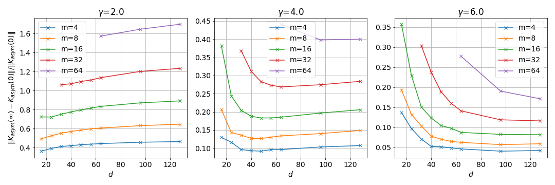
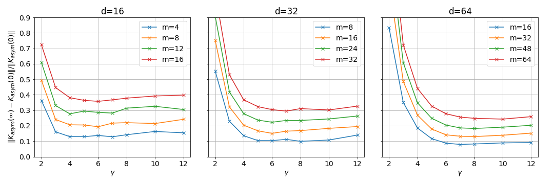
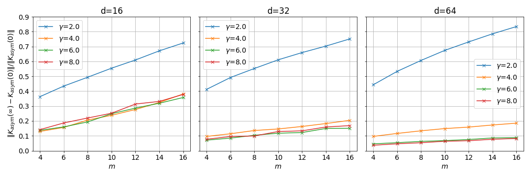
Figure 5: Relative change of ${\boldsymbol{\mathbf{K}}_{\mathsf{asym}}}(t)$ in the QNN asymptotic dynamics for varying system dimension $d$, scaling factor $\gamma$ and number of training samples $m$. $\boldsymbol{\mathbf{K}}_{asym}(t)$ changes significantly ($\geq 5\%$) throughout training.

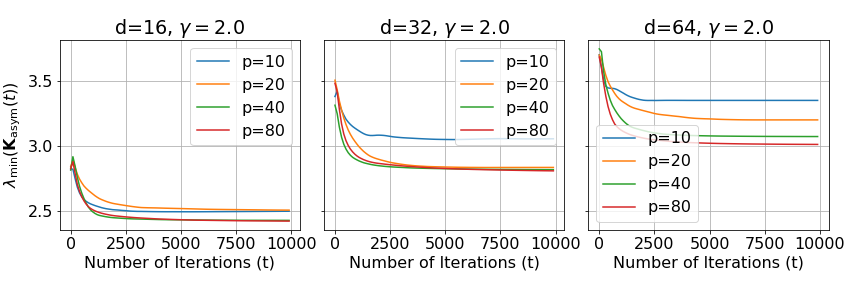
Figure 6: Change of the $\lambda_{\min}({\boldsymbol{\mathbf{K}}_{\mathsf{asym}}}(t))$ during the training in QNNs with $m=4,\gamma=2.0$ and varying $d$.

References

- Allen-Zhu et al. (2019) Z. Allen-Zhu, Y. Li, and Z. Song. A convergence theory for deep learning via over-parameterization. In K. Chaudhuri and R. Salakhutdinov, editors, Proceedings of the 36th International Conference on Machine Learning, volume 97 of Proceedings of Machine Learning Research, pages 242–252. PMLR, 09–15 Jun 2019. URL https://proceedings.mlr.press/v97/allen-zhu19a.html.
- Anschuetz (2022) E. R. Anschuetz. Critical points in quantum generative models. In International Conference on Learning Representations, 2022. URL https://openreview.net/forum?id=2f1z55GVQN.
- Anschuetz and Kiani (2022) E. R. Anschuetz and B. T. Kiani. Quantum variational algorithms are swamped with traps. Nature Communications, 13(1):1–10, 2022.
- Arora et al. (2019) S. Arora, S. S. Du, W. Hu, Z. Li, R. R. Salakhutdinov, and R. Wang. On exact computation with an infinitely wide neural net. In H. Wallach, H. Larochelle, A. Beygelzimer, F. d'Alché-Buc, E. Fox, and R. Garnett, editors, Advances in Neural Information Processing Systems, volume 32. Curran Associates, Inc., 2019. URL https://proceedings.neurips.cc/paper_files/paper/2019/file/dbc4d84bfcfe2284ba11beffb853a8c4-Paper.pdf.
- Bietti and Mairal (2019) A. Bietti and J. Mairal. On the inductive bias of neural tangent kernels. Advances in Neural Information Processing Systems, 32, 2019.
- Canatar et al. (2021) A. Canatar, B. Bordelon, and C. Pehlevan. Spectral bias and task-model alignment explain generalization in kernel regression and infinitely wide neural networks. Nature communications, 12(1):1–12, 2021.
- Chakrabarti et al. (2019) S. Chakrabarti, H. Yiming, T. Li, S. Feizi, and X. Wu. Quantum wasserstein generative adversarial networks. Advances in Neural Information Processing Systems, 32, 2019.
- Chen et al. (2020) Z. Chen, Y. Cao, Q. Gu, and T. Zhang. A generalized neural tangent kernel analysis for two-layer neural networks. Advances in Neural Information Processing Systems, 33:13363–13373, 2020.
- Chizat et al. (2019) L. Chizat, E. Oyallon, and F. Bach. On lazy training in differentiable programming. In Advances in Neural Information Processing Systems, volume 32. Curran Associates, Inc., 2019. URL https://proceedings.neurips.cc/paper/2019/file/ae614c557843b1df326cb29c57225459-Paper.pdf.
- Collins and Śniady (2006) B. Collins and P. Śniady. Integration with respect to the haar measure on unitary, orthogonal and symplectic group. Communications in Mathematical Physics, 264(3):773–795, 2006.
- Cong et al. (2019) I. Cong, S. Choi, and M. D. Lukin. Quantum convolutional neural networks. Nature Physics, 15(12):1273–1278, 2019.
- Du et al. (2022) Y. Du, Y. Yang, D. Tao, and M.-H. Hsieh. Demystify problem-dependent power of quantum neural networks on multi-class classification. arXiv preprint arXiv:2301.01597, 2022.
- Dunjko and Briegel (2018) V. Dunjko and H. J. Briegel. Machine learning and artificial intelligence in the quantum domain: a review of recent progress. Reports on Progress in Physics, 81(7):074001, jun 2018. doi: 10.1088/1361-6633/aab406. URL https://doi.org/10.1088/1361-6633/aab406.
- Farhi et al. (2020) E. Farhi, H. Neven, et al. Classification with quantum neural networks on near term processors. Quantum Review Letters, 1(2 (2020)):10–37686, 2020.
- Horn and Johnson (2012) R. A. Horn and C. R. Johnson. Matrix analysis. Cambridge university press, 2012.
- Huang et al. (2021) H.-Y. Huang, M. Broughton, M. Mohseni, R. Babbush, S. Boixo, H. Neven, and J. R. McClean. Power of data in quantum machine learning. Nature Communications, 12(1), may 2021. doi: 10.1038/s41467-021-22539-9. URL https://doi.org/10.1038%2Fs41467-021-22539-9.
- Jacot et al. (2018) A. Jacot, F. Gabriel, and C. Hongler. Neural tangent kernel: Convergence and generalization in neural networks. Advances in neural information processing systems, 31, 2018.
- Larocca et al. (2021) M. Larocca, N. Ju, D. García-Martín, P. J. Coles, and M. Cerezo. Theory of overparametrization in quantum neural networks. arXiv preprint arXiv:2109.11676, 2021.
- Liu et al. (2022a) J. Liu, K. Najafi, K. Sharma, F. Tacchino, L. Jiang, and A. Mezzacapo. An analytic theory for the dynamics of wide quantum neural networks. arXiv preprint arXiv:2203.16711, 2022a.
- Liu et al. (2022b) J. Liu, F. Tacchino, J. R. Glick, L. Jiang, and A. Mezzacapo. Representation learning via quantum neural tangent kernels. PRX Quantum, 3(3):030323, 2022b.
- Livni et al. (2014) R. Livni, S. Shalev-Shwartz, and O. Shamir. On the computational efficiency of training neural networks. In Z. Ghahramani, M. Welling, C. Cortes, N. Lawrence, and K. Weinberger, editors, Advances in Neural Information Processing Systems, volume 27. Curran Associates, Inc., 2014. URL https://proceedings.neurips.cc/paper/2014/file/3a0772443a0739141292a5429b952fe6-Paper.pdf.
- Lloyd and Weedbrook (2018) S. Lloyd and C. Weedbrook. Quantum generative adversarial learning. Physical Review Letters, 121(4), jul 2018. doi: 10.1103/physrevlett.121.040502. URL https://doi.org/10.1103%2Fphysrevlett.121.040502.
- McClean et al. (2018) J. R. McClean, S. Boixo, V. N. Smelyanskiy, R. Babbush, and H. Neven. Barren plateaus in quantum neural network training landscapes. Nature communications, 9(1):1–6, 2018.
- Oymak and Soltanolkotabi (2020) S. Oymak and M. Soltanolkotabi. Toward moderate overparameterization: Global convergence guarantees for training shallow neural networks. IEEE Journal on Selected Areas in Information Theory, 1(1):84–105, 2020.
- Paszke et al. (2019) A. Paszke, S. Gross, F. Massa, A. Lerer, J. Bradbury, G. Chanan, T. Killeen, Z. Lin, N. Gimelshein, L. Antiga, et al. Pytorch: An imperative style, high-performance deep learning library. Advances in neural information processing systems, 32, 2019.
- Preskill (2018) J. Preskill. Quantum computing in the nisq era and beyond. Quantum, 2:79, 2018.
- Ragone et al. (2022) M. Ragone, P. Braccia, Q. T. Nguyen, L. Schatzki, P. J. Coles, F. Sauvage, M. Larocca, and M. Cerezo. Representation theory for geometric quantum machine learning. arXiv preprint arXiv:2210.07980, 2022.
- Romero et al. (2017) J. Romero, J. P. Olson, and A. Aspuru-Guzik. Quantum autoencoders for efficient compression of quantum data. Quantum Science and Technology, 2(4):045001, aug 2017. doi: 10.1088/2058-9565/aa8072. URL https://doi.org/10.1088/2058-9565/aa8072.
- Russell et al. (2017) B. Russell, H. Rabitz, and R.-B. Wu. Control landscapes are almost always trap free: a geometric assessment. Journal of Physics A: Mathematical and Theoretical, 50(20):205302, apr 2017. doi: 10.1088/1751-8121/aa6b77. URL https://dx.doi.org/10.1088/1751-8121/aa6b77.
- Schuld and Killoran (2019) M. Schuld and N. Killoran. Quantum machine learning in feature hilbert spaces. Physical review letters, 122(4):040504, 2019.
- Shirai et al. (2021) N. Shirai, K. Kubo, K. Mitarai, and K. Fujii. Quantum tangent kernel. arXiv preprint arXiv:2111.02951, 2021.
- Tropp (2012) J. A. Tropp. User-friendly tail bounds for sums of random matrices. Foundations of computational mathematics, 12(4):389–434, 2012.
- Vershynin (2010) R. Vershynin. Introduction to the non-asymptotic analysis of random matrices. arXiv preprint arXiv:1011.3027, 2010.
- Wang et al. (2022) X. Wang, J. Liu, T. Liu, Y. Luo, Y. Du, and D. Tao. Symmetric pruning in quantum neural networks. arXiv preprint arXiv:2208.14057, 2022.
- You and Wu (2021) X. You and X. Wu. Exponentially many local minima in quantum neural networks. In International Conference on Machine Learning, pages 12144–12155. PMLR, 2021.
- You et al. (2022) X. You, S. Chakrabarti, and X. Wu. A convergence theory for over-parameterized variational quantum eigensolvers. arXiv:2205.12481, 2022.
- Zoufal et al. (2019) C. Zoufal, A. Lucchi, and S. Woerner. Quantum generative adversarial networks for learning and loading random distributions. npj Quantum Information, 5(1), nov 2019. doi: 10.1038/s41534-019-0223-2. URL https://doi.org/10.1038%2Fs41534-019-0223-2.