Scale invariance and critical balance in electrostatic drift-kinetic turbulence

Abstract

The equations of electrostatic drift kinetics are observed to possess a symmetry associated with their intrinsic scale invariance. Under the assumptions of spatial periodicity, stationarity, and locality, this symmetry implies a particular scaling of the turbulent heat flux with the system’s parallel size, from which its scaling with the equilibrium temperature gradient can be deduced under some additional assumptions. This macroscopic transport prediction is then confirmed numerically for a reduced model of electron-temperature-gradient-driven turbulence in slab geometry. The system realises this scaling through a turbulent cascade from large to small perpendicular spatial scales. The route of this cascade through wavenumber space (i.e., the relationship between parallel and perpendicular scales in the inertial range) is shown to be determined by a balance between nonlinear-decorrelation and parallel-dissipation timescales. This type of “critically balanced” cascade, which maintains a constant energy flux despite the presence of parallel dissipation throughout the inertial range (as well as order-unity dissipative losses at the outer scale) is expected to be a generic feature of plasma turbulence. The outer scale of the turbulence, on which the turbulent heat flux depends, is determined by the breaking of drift-kinetic scale invariance due to the existence of large-scale parallel inhomogeneity (the parallel system size).

1 Introduction

In many plasmas, energy is injected into the system on some large, system-specific macroscale (the “outer scale”). In order for such a system to reach a steady state, this energy must be dissipated. The usual route to this dissipation in kinetic plasmas is via a turbulent cascade of this energy to fine scales in both position and velocity space, where it is eventually thermalised by collisions (the “inner scale”). Given that there is often a large separation between these inner and outer scales [such as in, e.g., astrophysical systems, where energy is often injected by magnetohydrodynamic (MHD) instabilities], many studies of plasma turbulence are able to consider the dynamics of this turbulent cascade separately from the specific mechanisms of injection, simply assuming that there is some energy arriving from large scales that needs to be processed (see, e.g., Schekochihin et al. 2009 and references therein).

There are, however, a variety of plasma systems for which such a scale separation is not a priori obvious. This is often due to the existence of gradients associated with an equilibrium (whether gravitational or magnetic) that, thermodynamically speaking, provide sources of free energy for unstable, microscale perturbations that can engender a turbulent cascade well below the usual macroscopic outer scale. In fact, the most (linearly) unstable perturbations in such systems often occur at the smallest scales. This is the case in tokamaks, in which the turbulent heat and particle transport is dominated by the (microscale) instabilities driven by the gradients of the plasma pressure between the inner core of the tokamak and its edge. The most important of these instabilities are the ion-temperature gradient (ITG) (see, e.g., Waltz, 1988; Cowley et al., 1991; Kotschenreuther et al., 1995a) and electron-temperature gradient (ETG) ones (see, e.g., Liu, 1971; Lee et al., 1987; Dorland et al., 2000; Jenko et al., 2000). The relationship between the macroscopic scales associated with the plasma equilibrium and the microscopic scales on which turbulent fluctuations grow — and how the interaction between these two scales determines the heat and particle transport properties of the confined plasma — remains a topic of active research and great consequence.

In this paper, we consider electrostatic, drift-kinetic plasma turbulence — applicable to many regimes of tokamak operation — with a particular focus on the connection between its macroscopic transport properties and microscale dynamics. In the presence of constant perpendicular equilibrium gradients, it is observed that the equations of electrostatic drift kinetics possess a symmetry associated with their intrinsic scale invariance, in both the collisionless and collisional limits. We then show that this symmetry implies a particular scaling of the turbulent heat flux with equilibrium-scale quantities, in particular the parallel system size, provided one can assume spatial periodicity, stationarity (that the system has reached a statistical steady state), and locality (that the heat flux is independent of the system’s perpendicular size, as it should be for any valid local model of plasma turbulence, provided its perpendicular size is large enough). This macroscopic transport prediction is then confirmed numerically in the context of an electron-scale, collisional model of electrostatic turbulence driven by the ETG instability in slab geometry. The choice to focus on ETG-driven turbulence was motivated, in part, by the fact that, despite significant recent progress (see, e.g., Ren et al., 2017; Hatch et al., 2019; Parisi et al., 2020; Guttenfelder et al., 2021, 2022; Parisi et al., 2022; Chapman-Oplopoiou et al., 2022; Field et al., 2023), the saturation of such turbulence remains significantly less well-understood than its ITG cousin.

Further consideration of the microscale dynamics of our system of equations reveals that this heat flux scaling is enabled by a critically-balanced, Kolmogorov (1941) style cascade of energy from large to small spatial scales. The (approximately) constant flux of energy is that which survives the parallel dissipation present at the largest scales due, in our model, to thermal conduction. The existence of this parallel dissipation is also shown to play a key role in determining the saturated state of the system, limiting the cascade of free energy in wavenumber space. The outer scale of the turbulence is found to be determined by the breaking of the drift-kinetic scale invariance due to the existence of some large-scale parallel inhomogeneity, viz., the parallel system size, rather than by the smallest scales on which the ETG instability’s growth rate peaks. It is thus the largest scales that are the most important in determining the saturated amplitudes to which the fluctuations grow, and the resultant turbulent transport. This is the first detailed demonstration of a critically balanced cascade in a temperature-gradient-driven plasma system since Barnes et al. (2011) proposed such a cascade for ITG turbulence.

The rest of this paper is organised as follows. In section 2, the scaling of the turbulent heat flux with parallel system size is derived from considerations of the scale invariance of the electrostatic drift-kinetic system of equations. Our model system of fluid equations is introduced in section 3, and the aforementioned heat flux scaling is verified in section 4. The dynamics of the inertial range are considered extensively in section 5, including the free-energy budget (section 5.1), the existence of a constant-flux cascade and dynamical critical balance (section 5.2), the nature of the outer scale (section 5.3), the two-dimensional $(k_{\perp},k_{\parallel})$ spectra (section 5.4), and the perpendicular isotropy in wavenumber space (section 5.5). Lastly, we summarise our results and generic conclusions in section 6, and discuss the limits of their applicability to plasma systems in which finite-Larmor-radius (FLR) or electromagnetic effects are thought to be important.

2 Electrostatic drift-kinetic scale invariance

For systems adequately described by electrostatic drift kinetics, the heat flux through some volume $V$ is given by

$$Q=\sum_{s}Q_{s},\quad Q_{s}=n_{0s}T_{0s}\int\frac{\mathrm{d}^{3}{\boldsymbol{r}}}{V}\>\left({\boldsymbol{v}}_{E}\cdot{\boldsymbol{\nabla}}x\right)\frac{\delta T_{s}}{T_{0s}},$$ (1)

where ${\boldsymbol{\nabla}}x$ is the (radial) direction of the equilibrium gradients, $n_{0s}$ and $T_{0s}$ are the equilibrium density and temperature, respectively, of species $s$, $\delta T_{s}$ is the corresponding temperature perturbation [see eq. 91], and

$${\boldsymbol{v}}_{E}=\frac{c}{B_{0}}{\boldsymbol{b}}_{0}\times{\boldsymbol{\nabla}}\phi,$$ (2)

is the ${\boldsymbol{E}}\times{\boldsymbol{B}}$ drift velocity due to the perturbed electrostatic potential $\phi$, $B_{0}$ and ${\boldsymbol{b}}_{0}$ being the magnitude and direction of the equilibrium magnetic field, respectively. In what follows, $L_{n_{s}}$ and $L_{T_{s}}$ denote the characteristic scale lengths associated with the gradients of the equilibrium density and temperature, respectively, while the equilibrium energy scale of species $s$ is set by its thermal speed $v_{{\rm th}s}=\sqrt{2T_{0s}/m_{s}}$, with $m_{s}$ being the particle mass.

In appendix A, we show that, for constant perpendicular equilibrium gradients, the electrostatic, drift-kinetic system of equations is invariant under a particular one-parameter transformation. Under this transformation, the perturbed temperature and electrostatic potential transform as, for any $\lambda$,

$$\delta\tilde{T}_{s}=\lambda^{2}\delta T_{s}(x/\lambda^{2},y/\lambda^{2},z/\lambda^{2/\alpha},t/\lambda^{2}),\quad\tilde{\phi}=\lambda^{2}\phi(x/\lambda^{2},y/\lambda^{2},z/\lambda^{2/\alpha},t/\lambda^{2}).$$ (3)

Here, $x$, $y$ and $z$ are the radial, binormal and parallel coordinates, respectively, the tildes indicate the transformed fields, and $\alpha=1,2$ in the collisionless and collisional limits, respectively. We have assumed that the collisional limit corresponds to the case where the frequency of the perturbations $\omega$ is comparable to rate of thermal conduction, but much smaller than $\nu_{ss^{\prime}}$, the characteristic collision frequency between species $s$ and $s^{\prime}$, viz., $\omega\sim(k_{\parallel}v_{{\rm th}s})^{2}/\nu_{ss^{\prime}}\ll\nu_{ss^{\prime}}$, as in Braginskii (1965) (where $k_{\parallel}$ is the characteristic wavenumber of the perturbations along the direction of the equilibrium magnetic field). Mathematically, the existence of the symmetry eq. 3 is a consequence of the scale invariance of electrostatic drift kinetics: in the absence of finite-Larmor-radius effects associated with $\rho_{s}$ — the Larmor radius of species $s$, manifest in the gyroaverages and the resultant Bessel functions appearing in gyrokinetics (see, e.g., Abel et al., 2013) — there is no intrinsic perpendicular scale in the system, with nothing to distinguish any perpendicular scale from any other.

Under eq. 3, and noting the presence of the perpendicular derivative in eq. 2, the heat flux eq. 1 transforms as

$$\tilde{Q}_{s}=\lambda^{2}Q_{s}.$$ (4)

Now suppose that our original solutions for $\delta T_{s}$ and $\phi$ were periodic in $x$, $y$ and $z$ with domain sizes $L_{x}$, $L_{y}$, and $L_{\parallel}$, respectively. Then, the transformed solutions $\delta\tilde{T}_{s}$ and $\tilde{\phi}$ are still periodic in $x$, $y$ and $z$, except with domain sizes $\lambda^{2}L_{x}$, $\lambda^{2}L_{y}$, and $\lambda^{2/\alpha}L_{\parallel}$, implying that

$$\tilde{Q}_{s}(\lambda^{2}L_{x},\lambda^{2}L_{y},\lambda^{2/\alpha}L_{\parallel},t/\lambda^{2})=\lambda^{2}Q_{s}(L_{x},L_{y},L_{\parallel},t).$$ (5)

The heat flux will, of course, depend on other parameters of the system, e.g., equilibrium gradients and collisionality. These, however, remain unchanged under the transformation (by construction), and so we did not write them explicitly in eq. 5. In a strongly magnetised (gyrokinetic) plasma, structures generated by the turbulent fluctuations are ordered comparable to the equilibrium scales in the parallel direction ($k_{\parallel}^{-1}\sim L_{\parallel}\sim L_{T_{s}}$), but remain microscopic in the perpendicular direction ($k_{\perp}^{-1}\sim\rho_{s}$). This means that, as the perpendicular domain size $L_{\perp}$ (ordered as $L_{\perp}\sim L_{x}\sim L_{y}\sim\rho_{s}$) is increased, there must come a point at which the turbulence, and the resultant heat flux, become independent of the perpendicular domain size; if this were not the case, then the heat flux would diverge as $L_{\perp}/\rho_{s}\rightarrow\infty$, implying that drift kinetics is not a valid local model of the plasma. We thus assume that the heat flux is independent of the perpendicular domain size, viz., independent of $L_{x}$ and $L_{y}$. We also assume that the heat flux is independent of time, in the sense that it has been able to reach a statistical steady state. Then, given that $\lambda$ can be chosen arbitrarily, eq. 5 directly implies that

$$Q_{s}\propto L_{\parallel}^{\alpha},$$ (6)

where once again $\alpha=1,2$ in the collisionless and collisional limits, respectively. Physically, $L_{\parallel}$ can be thought of either as a measure of a quantity analogous to the connection length $2\pi qR$ in tokamak geometry (where $q$ is the safety factor and $R$ the major radius) or, in the absence of any other gradients, as a proxy for the temperature-gradient scale length. The latter follows from dimensional analysis: without loss of generality,

$$\frac{Q_{s}}{Q_{\text{gB}s}}=\left(\frac{L_{\parallel}}{L_{T_{s}}}\right)^{\alpha}G\left(\nu_{*s},\frac{L_{n_{s}}}{L_{T_{s}}},\frac{R}{L_{T_{s}}},\dots\right),$$ (7)

where $Q_{\text{gB}s}=n_{0s}T_{0s}v_{{\rm th}s}(\rho_{s}/L_{T_{s}})^{2}$ is the “gyro-Bohm” heat flux, $G$ is an unknown function, $\nu_{*s}=(L_{T}/v_{{\rm th}s})\sum_{s^{\prime}}\nu_{ss^{\prime}}$ is the normalised collisionality, and “$\dots$” stands for other equilibrium parameters on which the heat flux can depend, normalised, wherever a scale is required, using the temperature-gradient scale length $L_{T_{s}}$. If the dependence of $G$ on these other parameters can be ignored in eq. 7 — due either to the absence of other gradients in, e.g., slab geometry, or the system being driven far above marginality where such dependences are typically weak — then the scaling of the heat flux with $L_{T_{s}}$ follows directly from its dependence on $L_{\parallel}$.

This is perhaps a surprising result. Under the assumptions that the system is spatially periodic, that it is able to reach a statistical steady state (stationarity), and that the heat flux is independent of the system’s perpendicular size, as it should be for any valid local model of a plasma (spatial locality), the scale invariance of electrostatic drift kinetics enforces the scaling eq. 6, which is a non-trivial prediction about the scaling of the heat flux with equilibrium parameters. The key physics question, then, is how the system organises itself in order to obey this scaling. Namely, it has to find a way to process the free energy injected by the equilibrium gradients at a steady rate (stationarity) and to choose a spatial scale independent of $L_{\perp}$ (locality). In the remainder of this paper, we investigate a particular example of a system that should exhibit this scaling, being derived in an asymptotic limit of electrostatic drift kinetics, and find that a critically balanced, Kolmogorov (1941)-style cascade of energy from large to small spatial scales is the dynamical means by which the formal constraint imposed by eq. 3 is realised.

3 Collisional fluid model

Fluid models are capable of providing remarkable insight about the dynamics of more general physical systems, while retaining the advantage of being (comparatively) simple to handle both numerically and analytically (e.g., Cowley et al., 1991; Newton et al., 2010; Ivanov et al., 2020, 2022). The ITG and ETG instabilities in tokamaks rely on destabilisation mechanisms that are fundamentally fluid (i.e., they are not resonant instabilities) and, even in kinetic regimes, they tend to be described adequately by fluid closures (Hammett & Perkins, 1990; Hammett et al., 1992, 1993; Dorland & Hammett, 1993; Beer & Hammett, 1996; Snyder et al., 1997). Here we consider an electron-scale, collisional ($\nu_{*e}\gg 1$) fluid model of electrostatic turbulence driven by the electron-temperature gradient. Despite its simplicity, we expect that many of the results reported below are qualitatively applicable to more general turbulent plasma systems.

We take the local plasma equilibrium to be that of conventional slab gyrokinetics (see, e.g., Howes et al., 2006). The (homogeneous) equilibrium magnetic field is in the ${\boldsymbol{b}}_{0}=\hat{{\boldsymbol{z}}}$ direction; perturbations to both its direction and magnitude are assumed negligible, consistent with the electrostatic limit. The electric field is then related to the electrostatic potential $\phi$ by ${\boldsymbol{E}}=-{\boldsymbol{\nabla}}\phi$, and has no mean part. The equilibrium profile of the electron temperature $T_{0e}$ varies radially, with the scale length

$$L_{T}^{-1}\equiv L_{T_{e}}^{-1}=-\frac{1}{T_{0e}}\frac{\mathrm{d}T_{0e}}{\mathrm{d}x},$$ (8)

which is assumed to be constant over the domain of the system. The equilibrium gradients of density and ion temperature are assumed to be negligibly small. The omission of an equilibrium density gradient means that our system will be unstable for any finite $L_{T}^{-1}$; the resultant dynamics can thus be considered to apply to a plasma driven strongly above marginality (unlike the cases considered in, e.g., Guttenfelder et al. 2021; Hatch et al. 2022; Chapman-Oplopoiou et al. 2022; Field et al. 2023, where a strong dependence of the heat flux on the equilibrium density gradient was identified).

3.1 Moment equations

With this local equilibrium, we derive, in appendix B, evolution equations for the density ($\delta n_{e}$), parallel velocity ($u_{\parallel e}$), and temperature ($\delta T_{e}$) perturbations of the electrons:

$$\frac{\mathrm{d}}{\mathrm{d}t}\frac{\delta n_{e}}{n_{0e}}+\frac{\partial u_{\parallel e}}{\partial z}=0,$$ (9)

$$\frac{\nu_{ei}}{c_{1}}\frac{u_{\parallel e}}{v_{{\rm th}e}}=-\frac{v_{{\rm th}e}}{2}\frac{\partial}{\partial z}\left[\frac{\delta n_{e}}{n_{0e}}-\varphi+\left(1+\frac{c_{2}}{c_{1}}\right)\frac{\delta T_{e}}{T_{0e}}\right],$$ (10)

$$\frac{\mathrm{d}}{\mathrm{d}t}\frac{\delta T_{e}}{T_{0e}}+\frac{2}{3}\frac{\partial}{\partial z}\frac{\delta q_{e}}{n_{0e}T_{0e}}+\frac{2}{3}\left(1+\frac{c_{2}}{c_{1}}\right)\frac{\partial u_{\parallel e}}{\partial z}=-\frac{\rho_{e}v_{{\rm th}e}}{2L_{T}}\frac{\partial\varphi}{\partial y}.$$ (11)

Let us discuss what these equations represent.

Equation eq. 9 is the familiar continuity equation. It describes the advection of the density perturbation by the ${\boldsymbol{E}}\times{\boldsymbol{B}}$ motion eq. 2 of the electrons:

$$\frac{\mathrm{d}}{\mathrm{d}t}=\frac{\partial}{\partial t}+{\boldsymbol{v}}_{E}\cdot{\boldsymbol{\nabla}}_{\perp}=\frac{\partial}{\partial t}+\frac{\rho_{e}v_{{\rm th}e}}{2}\left\{\varphi,\dots\right\},\quad\varphi=\frac{e\phi}{T_{0e}},$$ (12)

and their compression or rarefaction due to the perturbed electron flow $u_{\parallel e}{\boldsymbol{b}}_{0}$ parallel to the equilibrium magnetic-field direction.

This flow velocity is determined (instantaneously) from a balance between the electron-ion frictional force — proportional to the electron-ion collision frequency $\nu_{ei}$ [see eq. 95] and appearing on the left-hand side of eq. 10 — and the forces on the right-hand side of eq. 10: the parallel pressure gradient, the electrostatic part of the parallel electric field, and the collisional ‘thermal forces’ (Braginskii, 1965; Helander & Sigmar, 2005), proportional to $c_{2}/c_{1}$, that arise due to the velocity dependence of the collision frequency associated with the Landau collision operator [see eq. 78]. The order-unity constants $c_{1}$, $c_{2}$ and $c_{3}$ [the latter appearing in eq. 13] arise from the inversion of said operator, and depend on the magnitude of the ion charge $Z$ [see eq. 129]: e.g., for $Z=1$, $c_{1}\approx 1.94$, $c_{2}\approx 1.39$ and $c_{3}\approx 3.16$, in agreement with Braginskii (1965).

The temperature perturbation in eq. 11 is advected by the local ${\boldsymbol{E}}\times{\boldsymbol{B}}$ flow eq. 2, again according to eq. 12, and is locally increased (or decreased) by compressional heating (or rarefaction cooling) due to $u_{\parallel e}$, as well as by the perturbed parallel collisional heat flux

$$\frac{\delta q_{e}}{n_{0e}T_{0e}}=-c_{3}\frac{v_{{\rm th}e}^{2}}{2\nu_{ei}}\frac{\partial}{\partial z}\frac{\delta T_{e}}{T_{0e}}$$ (13)

caused by the gradient of the temperature perturbation along the equilibrium magnetic field direction. The term on the right-hand side of eq. 11 is the familiar linear drive (advection of the equilibrium temperature profile by the perturbed ${\boldsymbol{E}}\times{\boldsymbol{B}}$ flow) responsible for extracting free energy from the equilibrium temperature gradient $L_{T}^{-1}$, defined in eq. 8.

Finally, the electron-density perturbation is related to the non-dimensionalised potential $\varphi$ via quasineutrality:

$$\frac{\delta n_{e}}{n_{0e}}=-\bar{\tau}^{-1}\varphi,\quad\bar{\tau}=\frac{\tau}{Z},$$ (14)

where $\tau=T_{0i}/T_{0e}$ is the ratio of the ion to electron equilibrium temperatures. This describes an adiabatic ion response at electron scales: at scales much smaller than their Larmor radius $\rho_{i}$, ions can be viewed as motionless rings of charge, and their density response is Boltzmann.

Given eq. 10, eq. 13 and eq. 14, we can contract our system to two evolution equations written entirely in terms of the electrostatic potential and temperature perturbations:

$$\frac{\partial}{\partial t}\bar{\tau}^{-1}\varphi-\frac{c_{1}v_{{\rm th}e}^{2}}{2\nu_{ei}}\frac{\partial^{2}}{\partial z^{2}}\left[\left(1+\frac{1}{\bar{\tau}}\right)\varphi-\left(1+\frac{c_{2}}{c_{1}}\right)\frac{\delta T_{e}}{T_{0e}}\right]=0,$$ (15)

$$\frac{\mathrm{d}}{\mathrm{d}t}\frac{\delta T_{e}}{T_{0e}}+\frac{2}{3}\frac{c_{1}v_{{\rm th}e}^{2}}{2\nu_{ei}}\frac{\partial^{2}}{\partial z^{2}}\left\{\left(1+\frac{1}{\bar{\tau}}\right)\left(1+\frac{c_{2}}{c_{1}}\right)\varphi-\left[\frac{c_{3}}{c_{1}}+\left(1+\frac{c_{2}}{c_{1}}\right)^{2}\right]\frac{\delta T_{e}}{T_{0e}}\right\}$$ (16)

$$\quad\quad\quad=-\frac{\rho_{e}v_{{\rm th}e}}{2L_{T}}\frac{\partial\varphi}{\partial y}.$$

Note that, due to the Boltzmann density response eq. 14, the advection term in eq. 15 has vanished, leaving a purely linear relationship between $\varphi$ and $\delta T_{e}$. The only nonlinearity left in the system is thus the advection of $\delta T_{e}$ by the ${\boldsymbol{E}}\times{\boldsymbol{B}}$ flow in eq. 16. Note that we find finite-amplitude nonlinear saturation in our numerical simulations despite this absence of any nonlinearity in eq. 15; see section 5.5 for further discussion. If finite magnetic drifts (associated with an inhomogeneous equilibrium magnetic field) are included in our model, however, we find that simulations fail to saturate; this is discussed in section 6 and appendix C.

3.2 Scale invariance

Given that eq. 15 and eq. 16 were derived in an asymptotic subsidiary limit of drift kinetics (see section B.3), they are necessarily invariant under the transformation eq. 3 with $\alpha=2$, and must therefore exhibit the scaling eq. 6 of the heat flux with parallel system size — this is confirmed numerically in section 4.2.

Physically, this scale invariance is a consequence of the fact that eq. 15 and eq. 16 are valid within the wavenumber range (see section B.1),

$$\sqrt{\beta_{e}}\ll k_{\parallel}L_{T}\ll 1,\quad\beta_{e}\frac{\lambda_{ei}}{L_{T}}\ll k_{\perp}\rho_{e}\ll\frac{\lambda_{ei}}{L_{T}},$$ (17)

i.e., at perpendicular scales much smaller that those at which electromagnetic effects become important (the “flux-freezing scale”; see Adkins et al., 2022), but much larger than those on which one encounters the effects of electron thermal diffusion due to the finite Larmor motion of the electrons (Hardman et al., 2022; Adkins, 2023) — both of these bring in a special perpendicular scale that would break the drift-kinetic scale invariance. In other words, eq. 15 and eq. 16 describe physics on scales

$$k_{\parallel}L_{T}\sim\sqrt{\sigma},\quad k_{\perp}\rho_{\perp}\sim 1,\quad\rho_{\perp}=\frac{\rho_{e}}{\sigma}\frac{L_{T}}{\lambda_{ei}},$$ (18)

where $\sigma$ is, formally, some arbitrary constant satisfying

$$\beta_{e}\ll\sigma\ll 1.$$ (19)

The fact that it should be arbitrary follows from the fact that there is no special scale within the wavenumber ranges eq. 18. Our normalisation of perpendicular and parallel wavenumbers in eq. 15-eq. 16 will thus also be arbitrary, up to the definition of $\sigma$.

3.3 Collisional slab ETG instability

Let us now summarise briefly the linear stability properties of the system of equations eq. 15-eq. 16. Linearising and Fourier-transforming these equations, one obtains the dispersion relation:

$$\omega^{2} +\left[1+\bar{\tau}+\frac{2}{3}\left(1+\frac{c_{2}}{c_{1}}\right)^{2}+\frac{2}{3}\frac{c_{3}}{c_{1}}\right]i{\omega_{\parallel}}\omega$$

$$\quad\quad\quad\quad-\left[\frac{2}{3}(1+\bar{\tau})\frac{c_{3}}{c_{1}}{\omega_{\parallel}}+\left(1+\frac{c_{2}}{c_{1}}\right)i\omega_{*e}\bar{\tau}\right]{\omega_{\parallel}}=0,$$ (20)

where we have introduced the characteristic parallel and perpendicular frequencies

$${\omega_{\parallel}}=c_{1}\frac{\left(k_{\parallel}v_{{\rm th}e}\right)^{2}}{2\nu_{ei}},\quad\omega_{*e}=\frac{k_{y}\rho_{e}v_{{\rm th}e}}{2L_{T}}.$$ (21)

These are, respectively, the rate of parallel thermal conduction and the drift frequency associated with the electron-temperature gradient. Note that the dispersion relation eq. 20 is quadratic in the frequency $\omega$ because the parallel velocity $u_{\parallel e}$ is determined instantaneously in terms of the other fields, by eq. 10, unlike in collisionless ETG theory (Adkins et al., 2022).

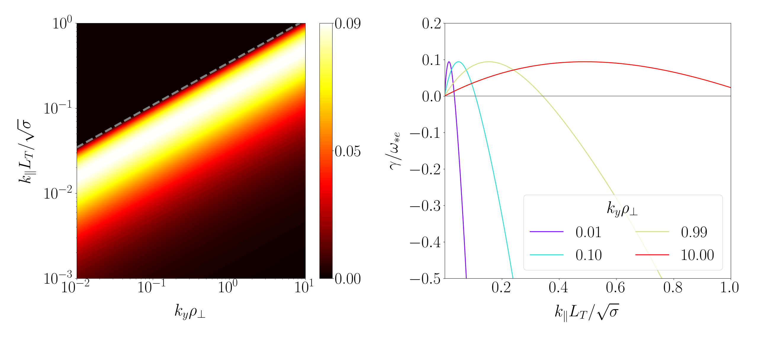
(a) $k_{x}\rho_{\perp}=0$	(b)

Figure 1: The growth rate of the collisional sETG instability: these are solutions to eq. 20 for $\tau=Z=1$, normalised to $\omega_{*e}$. Panel (a) is a contour plot of the positive growth rates ($\mathrm{Im}\>\omega>0)$ in the $(k_{y},k_{\parallel})$ plane; panel (b) shows cuts of the growth rate at constant $k_{y}\rho_{\perp}$, plotted as a function of $k_{\parallel}L_{T}/\sqrt{\sigma}$. The normalisations $\rho_{\perp}$ and $\sigma$ are defined in eq. 18. The stability boundary eq. 25 is indicated by grey dashed line in panel (a).

If we consider the limit of long parallel wavelengths, viz.,

$${\omega_{\parallel}}\ll\omega\ll\omega_{*e},$$ (22)

then the balance of the first and last terms in eq. 20 gives us

$$\omega^{2}=\left(1+\frac{c_{2}}{c_{1}}\right)i{\omega_{\parallel}}\omega_{*e}\bar{\tau}\quad\Rightarrow\quad\omega=\pm\frac{1+i\mathrm{sgn}(k_{y})}{\sqrt{2}}\left(1+\frac{c_{2}}{c_{1}}\right)^{1/2}\left({\omega_{\parallel}}|\omega_{*e}|\bar{\tau}\right)^{1/2}.$$ (23)

We recognise this as the collisional slab ETG (sETG) instability (Adkins et al., 2022), a cousin of the collisionless sETG (Lee et al., 1987).

The minimal set of equations that elucidate this process physically can be obtained from eq. 9-eq. 11 under the ordering eq. 22: using eq. 14 to express the density perturbations in terms of the electrostatic potential, we have:

$$\frac{\partial}{\partial t}\bar{\tau}^{-1}\varphi=\frac{\partial u_{\parallel e}}{\partial z},\quad\frac{\nu_{ei}}{c_{1}}u_{\parallel e}=-\left(1+\frac{c_{2}}{c_{1}}\right)\frac{v_{{\rm th}e}^{2}}{2}\frac{\partial}{\partial z}\frac{\delta T_{e}}{T_{0e}},\quad\frac{\mathrm{d}}{\mathrm{d}t}\frac{\delta T_{e}}{T_{0e}}=-\frac{\rho_{e}v_{{\rm th}e}}{2L_{T}}\frac{\partial\varphi}{\partial y}.$$ (24)

In this limit, the instability works as follows. Suppose that a small perturbation of the electron temperature is created with $k_{y}\neq 0$ and $k_{\parallel}\neq 0$, bringing the plasma from regions with higher $T_{0e}$ to those with lower $T_{0e}$ ($\delta T_{e}>0$), and vice-versa ($\delta T_{e}<0$). This temperature perturbation produces alternating hot and cold regions along the equilibrium magnetic field. The resulting perturbed temperature (and, therefore, pressure) gradients drive electron flows — determined instantaneously by the balance between the pressure gradient and collisional drag — from the hot regions to the cold regions [the second equation in eq. 24], giving rise to increased electron density in the cold regions [the first equation in eq. 24]. By quasineutrality, the electron density perturbation gives rise to an exactly equal ion density perturbation, and that, via the Boltzmann response eq. 14, creates an electric field that produces an ${\boldsymbol{E}}\times{\boldsymbol{B}}$ drift that in turn pushes hotter particles further into the colder region, and vice-versa [the third equation in eq. 24], reinforcing the initial temperature perturbation and thus completing the feedback loop required for the instability.

At short enough parallel wavelengths, the collisional sETG instability is quenched by rapid thermal conduction that leads to the damping of the associated temperature perturbation. To see this, we relax the assumption eq. 22 and consider the exact stability boundary of eq. 20, determined by the requirement that, assuming $\omega$ to be purely real, the real and imaginary parts of eq. 20 must vanish individually. The resultant equations can be straightforwardly combined to yield

$$\left(\frac{{\omega_{\parallel}}}{\omega_{*e}}\right)^{2}=\frac{\displaystyle\frac{3}{2}\left(1+\frac{c_{2}}{c_{1}}\right)^{2}\bar{\tau}^{2}}{\displaystyle(1+\bar{\tau})\frac{c_{3}}{c_{1}}\left[1+\bar{\tau}+\frac{2}{3}\left(1+\frac{c_{2}}{c_{1}}\right)^{2}+\frac{2}{3}\frac{c_{3}}{c_{1}}\right]^{2}}.$$ (25)

This is a curve $k_{y}\propto k_{\parallel}^{2}$ in wavenumber space, plotted as the grey dashed line in fig. 1(a). Above this line, corresponding to the limit ${\omega_{\parallel}}\gg\omega_{*e}$, all modes are purely damped due to rapid thermal conduction, as in fig. 1(b).

At any given $k_{y}$, the maximum growth rate of the collisional sETG is, therefore, reached when

$${\omega_{\parallel}}\sim\omega\sim\omega_{*e},$$ (26)

which is a balance between dissipation (through conduction) and energy injection due to the background temperature gradient. Indeed, maximising the growth rate from eq. 20 with respect to ${\omega_{\parallel}}$, one finds $\gamma_{\text{max}}=C(\tau,Z)\omega_{*e}$, where $C(\tau,Z)$ is a constant formally of order unity, e.g., $C(1,1)\approx 0.094$ [cf. the maximum values in fig. 1(b)]. The increase of the maximum growth rate of the sETG instability with the perpendicular wavenumber, $\omega_{*e}\propto k_{y}$, can only be checked by the effects of the electron perpendicular thermal diffusion due to finite electron Larmor motion, which, as discussed in section 3.2, occurs outside the range of wavenumbers in which eq. 15-eq. 16 are valid [see eq. 18], meaning that the instability grows fastest at the smallest perpendicular scales. The consequences of the intrinsic reliance of the collisional sETG on dissipative physics will be discussed in a nonlinear setting in section 5.1.

4 Numerical verification of scale invariance

4.1 Numerical setup

In what follows, the system eq. 15-eq. 16 is solved numerically in a triply periodic box of size $L_{x}\times L_{y}\times L_{\parallel}$ using a pseudo-spectral algorithm. Numerical integration is done in Fourier space ($N_{x}$, $N_{y}$ and $N_{\parallel}$ are the number of Fourier harmonics in the respective directions) with the nonlinear term calculated in real space using the 2/3 rule for de-aliasing (Orszag, 1971). We integrate the linear terms implicitly in time using the Crank-Nicolson method, while the nonlinear term is integrated explicitly using the Adams-Bashforth three-step method. This integration scheme is similar to the one implemented in the popular gyrokinetic code GS2 (Kotschenreuther et al., 1995b; Dorland et al., 2000).

Perpendicular hyperviscosity is introduced in order to provide an ultraviolet (large-wavenumber) cutoff for the instabilities, achieved by the replacement of the time derivative on the left-hand sides of eq. 15 and eq. 16 with

$$\frac{\partial}{\partial t}+(-1)^{N_{\nu}}\nu_{\perp}\left(\rho_{\perp}{\boldsymbol{\nabla}}_{\perp}\right)^{2{N_{\nu}}},$$ (27)

where $\nu_{\perp}$ is the “hypercollision” frequency and ${N_{\nu}}\geqslant 2$. With this change, our equations now depend only on the following dimensionless parameters: the perpendicular and parallel box sizes $L_{x}/\rho_{\perp}$, $L_{y}/\rho_{\perp}$ and $L_{\parallel}\sqrt{\sigma}/L_{T}$, the hyper-collision frequency $2\sigma(\rho_{\perp}/\rho_{e})^{2}\nu_{\perp}/\nu_{ei}$, and the power of the hyperviscous diffusion operator ${N_{\nu}}$. Convergence scans in $N_{x}$, $N_{y}$, and the perpendicular box size $L_{x}=L_{y}=L_{\perp}$ were carried out on a baseline simulation (see table 1) to ensure that the chosen resolution adequately captured the dynamics, and to verify that $L_{\perp}$ was large enough so that it did not significantly affect the simulation results, as was required for the arguments of section 2.

	$L_{x}/\rho_{\perp}$	$L_{y}/\rho_{\perp}$	$L_{\parallel}\sqrt{\sigma}/L_{T}$	$N_{x}$	$N_{y}$	$N_{\parallel}$	$2\sigma(\rho_{\perp}/\rho_{e})^{2}\nu_{\perp}/\nu_{ei}$	${N_{\nu}}$
Baseline	40	40	20	191	191	31	0.00050	2
Higher-resolution	40	40	20	383	383	63	0.00015	2

Table 1: The parameters used in the “baseline” and “higher-resolution” simulations. Both simulations had $\tau=Z=1$.

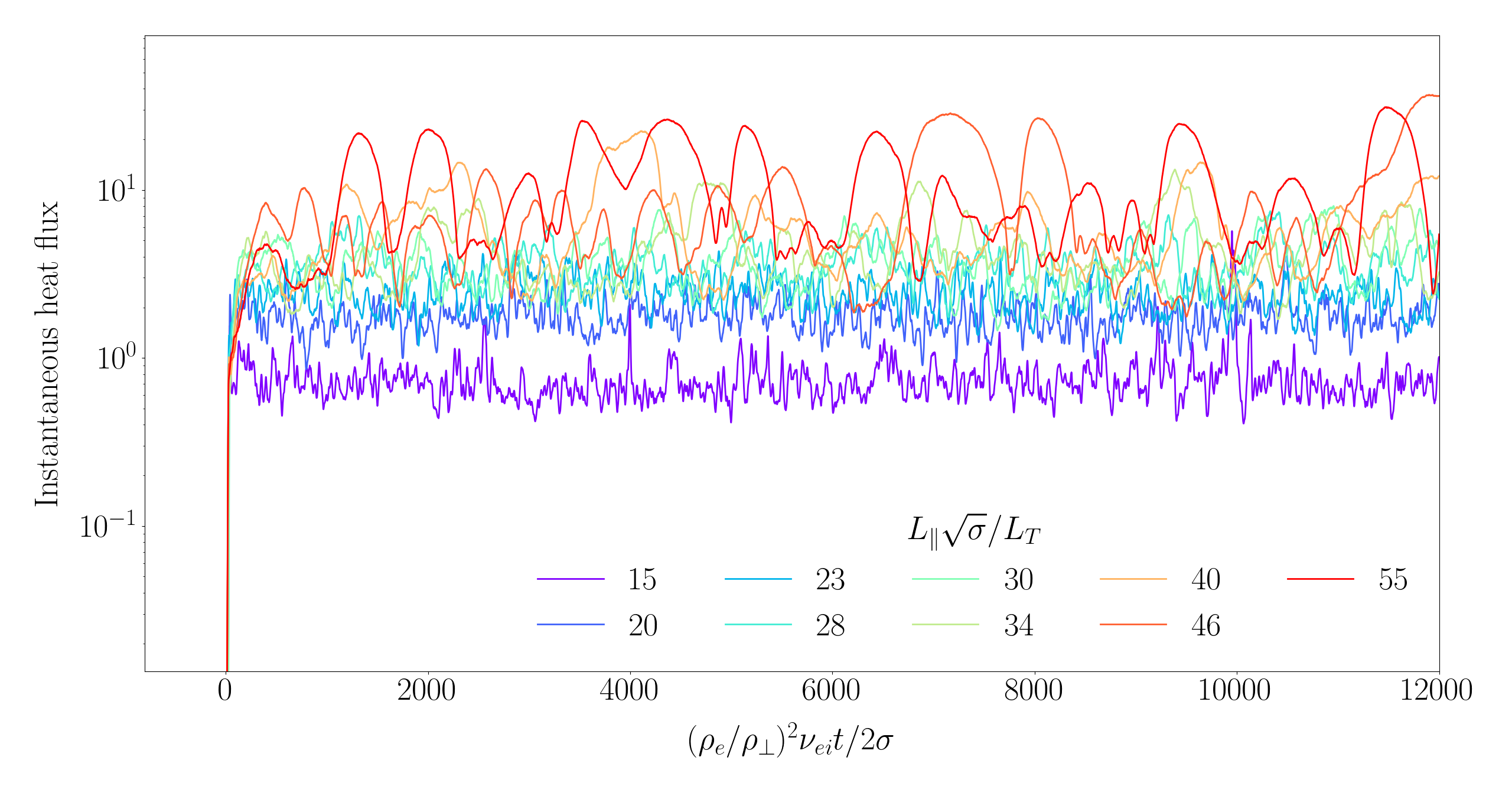
Figure 2: Time traces of the instantaneous heat flux from simulations in which $L_{\parallel}\sqrt{\sigma}/L_{T}$ was varied from 15 to 55, normalised to $(\rho_{\perp}/\rho_{e})Q_{\text{gB}e}$.

We have also found that our results do not depend on the specific details of the hyperviscosity, viz., on the values of $\nu_{\perp}$ and ${N_{\nu}}$. It can be viewed as a numerical tool that allows us to capture the dynamics of the system within a finite simulation domain and resolution, and is not intended to model a specific physical process. Ultimately, eq. 27 is a stand-in for the physical sinks of energy that exist at higher perpendicular wavenumbers. The fact that our results end up being independent of hyperviscosity is, however, significant. The addition of eq. 27 breaks the scale invariance associated with the transformation eq. 3, similarly to the way in which FLR effects would break the drift-kinetic scale invariance in the context of gyrokinetics, a point that we shall revisit in section 6. One could thus question the inevitability of obtaining the scaling of the heat flux eq. 6 in our system of equations with the modification eq. 27. Furthermore, the fact that the growth rate of the sETG instability peaks at a perpendicular scale determined by the hyperviscosity — since eq. 15 and eq. 16 contain no intrinsic perpendicular wavenumber cutoff — may also be a cause for concern, as the most unstable perpendicular scale is often thought to play a central role in determining turbulent transport. Both of these concerns can be dispelled by the realisation that the arguments of section 2 did not rely on the details of the state of the system at small perpendicular scales; indeed, the behaviour of the heat flux is determined by the parallel system size $L_{\parallel}$, which is manifestly an equilibrium-scale quantity. In section 5.2, we will show that this is a consequence of the fact that the outer scale is central in (dynamically) determining the transport and that this outer scale turns out to be independent of hyperviscosity.

4.2 Scan in $L_{\parallel}/L_{T}$

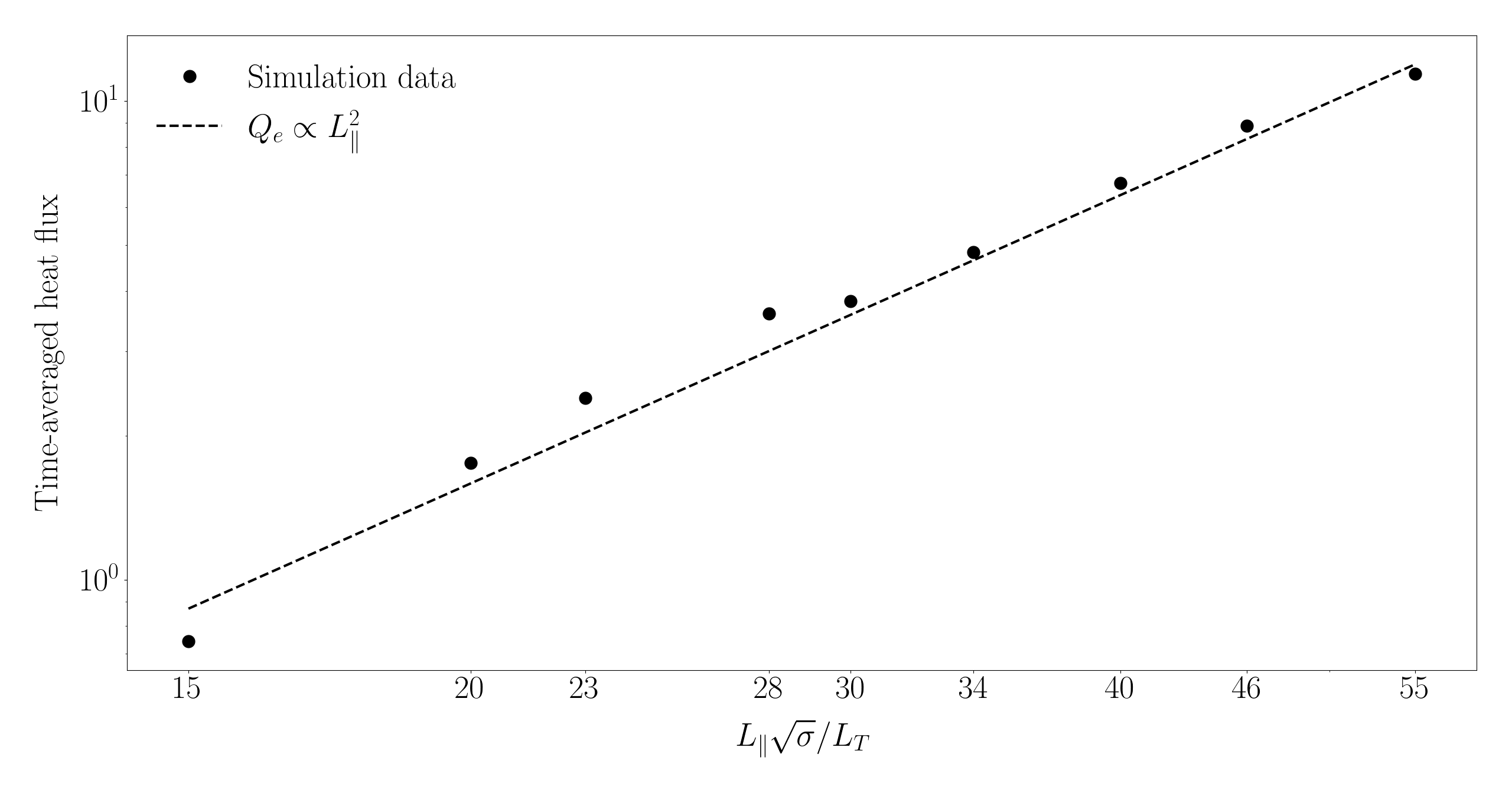
Figure 3: The scaling of the turbulent heat flux with $L_{\parallel}/L_{T}$, normalised to $(\rho_{\perp}/\rho_{e})Q_{\text{gB}e}$ and plotted against logarithmic axes. The points are the simulation data, while the theoretical prediction [see eq. 6] is shown by the dashed black line. A logarithmic fit to the data gives the slope of $2.02$.

In order to test the dependence of the turbulent heat flux on $L_{\parallel}$ predicted by eq. 6, we performed a series of simulations in which $L_{\parallel}\sqrt{\sigma}/L_{T}$ was varied between 15 and 55 at fixed parallel resolution (viz., fixed ratio of $L_{\parallel}\sqrt{\sigma}/L_{T}$ to $N_{\parallel}$), while keeping all other parameters the same as in the baseline simulation (see table 1). Each simulation was run to long enough times for it to reach saturation and stay in a statistically stationary state for a while, as can be seen from the time traces of the instantaneous heat fluxes plotted in fig. 2. That such a stationary state exists confirms one of the assumptions necessary for eq. 6, the other assumption, also confirmed numerically, being that this state is independent of $L_{x}$ and $L_{y}$.

In fig. 3, we plot the time average of the turbulent heat flux — as defined in eq. 1 for $s=e$, and normalised to $(\rho_{\perp}/\rho_{e})Q_{\text{gB}e}$, where $Q_{\text{gB}e}=n_{0e}T_{0e}v_{{\rm th}e}(\rho_{e}/L_{T})^{2}$ is the (electron) “gyro-Bohm” flux. It is clear that the simulation data agrees extremely well with the theoretical scaling eq. 6. This agreement, however, should not be a cause for complacency: though these results suggest that eq. 6 correctly predicts the transport, we would like to understand how the system manages this, i.e., how it contrives to satisfy the assumptions underpinning the prediction eq. 6. To explain this, we shall consider the dynamics in the inertial range. This is the subject of the following section.

5 Inertial-range dynamics

To ensure that we had sufficient numerical resolution to resolve adequately the dynamics of the inertial range, we conducted a “higher-resolution” simulation (see table 1), on which we shall now focus. Due to the computational demands introduced by the higher resolution, this simulation was run only up to 5000 $(\rho_{e}/\rho_{\perp})^{2}\nu_{ei}t/2\sigma$; this was sufficient to ensure that the heat flux had converged to a well-defined average value (see fig. 4).

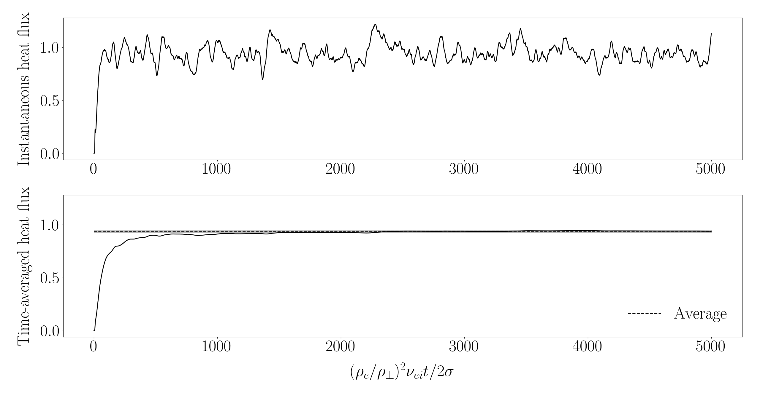
Figure 4: Turbulent heat flux in the higher-resolution simulation (see table 1), normalised to $(\rho_{\perp}/\rho_{e})Q_{\text{gB}e}$. The upper and lower panels show, respectively, the instantaneous and (rolling) time-averaged heat fluxes in solid black. The dashed horizontal line in the lower panel is the average value — as calculated over the entire time interval — while the transparent grey region around this value shows the error bar associated with the mean, calculated by means of a moving window average. The time-averaged heat flux converges to within the final error bar by $(\rho_{e}/\rho_{\perp})^{2}\nu_{ei}t/2\sigma\sim 2000$.

5.1 Free-energy budget

Magnetised plasma systems containing small perturbations around a Maxwellian equilibrium nonlinearly conserve free energy, which is a quadratic norm of the magnetic perturbations and the perturbations of the distribution functions of both ions and electrons away from the Maxwellian (see, e.g., Abel et al., 2013). In the system of equations that we are considering, the (normalised) free energy reduces to the form

$$\frac{W}{n_{0e}T_{0e}}=\int\frac{\mathrm{d}^{3}{\boldsymbol{r}}}{V}\left[\frac{1}{2\bar{\tau}}\left(1+\frac{1}{\bar{\tau}}\right)\varphi^{2}+\frac{3}{4}\frac{\delta T_{e}^{2}}{T_{0e}^{2}}\right].$$ (28)

The free energy is a nonlinear invariant, i.e., it is conserved by nonlinear interactions, but can be injected into the system by equilibrium gradients and is dissipated by collisions. It is straightforward to show from eq. 15 and eq. 16 [with the hyperviscosity eq. 27 appended] that the free-energy budget is

$$\frac{1}{n_{0e}T_{0e}}\frac{\mathrm{d}W}{\mathrm{d}t}=\varepsilon-D_{\parallel}-D_{\perp},$$ (29)

where

$$\varepsilon=\frac{1}{L_{T}}\int\frac{\mathrm{d}^{3}{\boldsymbol{r}}}{V}\>\frac{3}{2}\frac{\delta T_{e}}{T_{0e}}v_{Ex},\quad v_{Ex}=-\frac{\rho_{e}v_{{\rm th}e}}{2}\frac{\partial\varphi}{\partial y},$$ (30)

is the energy-injection rate from the equilibrium temperature gradient, and

$$D_{\parallel} =\frac{c_{1}v_{{\rm th}e}^{2}}{2\nu_{ei}}\int\frac{\mathrm{d}^{3}{\boldsymbol{r}}}{V}\left\{\left[\left(1+\frac{1}{\bar{\tau}}\right)\frac{\partial\varphi}{\partial z}-\left(1+\frac{c_{2}}{c_{1}}\right)\frac{\partial}{\partial z}\frac{\delta T_{e}}{T_{0e}}\right]^{2}+\frac{c_{3}}{c_{1}}\left(\frac{\partial}{\partial z}\frac{\delta T_{e}}{T_{0e}}\right)^{2}\right\},$$ (31)

$$D_{\perp} =\nu_{\perp}\int\frac{\mathrm{d}^{3}{\boldsymbol{r}}}{V}\left[\left(\rho_{\perp}^{{N_{\nu}}}{\boldsymbol{\nabla}}_{\perp}^{{N_{\nu}}}\varphi\right)^{2}+\frac{3}{2}\left(\rho_{\perp}^{{N_{\nu}}}{\boldsymbol{\nabla}}_{\perp}^{{N_{\nu}}}\frac{\delta T_{e}}{T_{0e}}\right)^{2}\right],$$ (32)

are the dissipation rates due to (parallel) thermal conduction and (perpendicular) hyperviscosity, respectively. The corresponding 1D perpendicular wavenumber spectrum of the energy injection is

$$\varepsilon_{{\boldsymbol{k}}}(k_{\perp})=2\pi k_{\perp}\int_{-\infty}^{\infty}\mathrm{d}k_{\parallel}\>\frac{3}{2}\mathrm{Re}\left<i\omega_{*e}\varphi_{{\boldsymbol{k}}}^{*}\frac{{\delta T_{e}}_{{\boldsymbol{k}}}}{T_{0e}}\right>,$$ (33)

while those of the parallel and perpendicular dissipation are

$${D_{\parallel}}_{{\boldsymbol{k}}}(k_{\perp}) =2\pi k_{\perp}\int_{-\infty}^{\infty}\mathrm{d}k_{\parallel}\left<\omega_{\parallel}\left[c_{1}\left|\left(1+\frac{1}{\bar{\tau}}\right)\varphi_{{\boldsymbol{k}}}-\left(1+\frac{c_{2}}{c_{1}}\right)\frac{{\delta T_{e}}_{{\boldsymbol{k}}}}{T_{0e}}\right|^{2}+c_{3}\left|\frac{{\delta T_{e}}_{{\boldsymbol{k}}}}{T_{0e}}\right|^{2}\right]\right>,$$ (34)

$${D_{\perp}}_{{\boldsymbol{k}}}(k_{\perp}) =2\pi k_{\perp}\int_{-\infty}^{\infty}\mathrm{d}k_{\parallel}\left<(k_{\perp}\rho_{\perp})^{2{N_{\nu}}}\nu_{\perp}\left(\left|\varphi_{{\boldsymbol{k}}}\right|^{2}+\frac{3}{2}\left|\frac{{\delta T_{e}}_{{\boldsymbol{k}}}}{T_{0e}}\right|^{2}\right)\right>.$$ (35)

In eq. 33, the asterisk denotes complex conjugation, and the angle brackets an ensemble average. Note that when analysing the output of simulations, we consider ensemble averages to be equal to time averages over a period following saturation and the establishment of a statistical steady state [e.g., after $(\rho_{e}/\rho_{\perp})^{2}\nu_{ei}t/2\sigma\sim 2000$ in fig. 2].

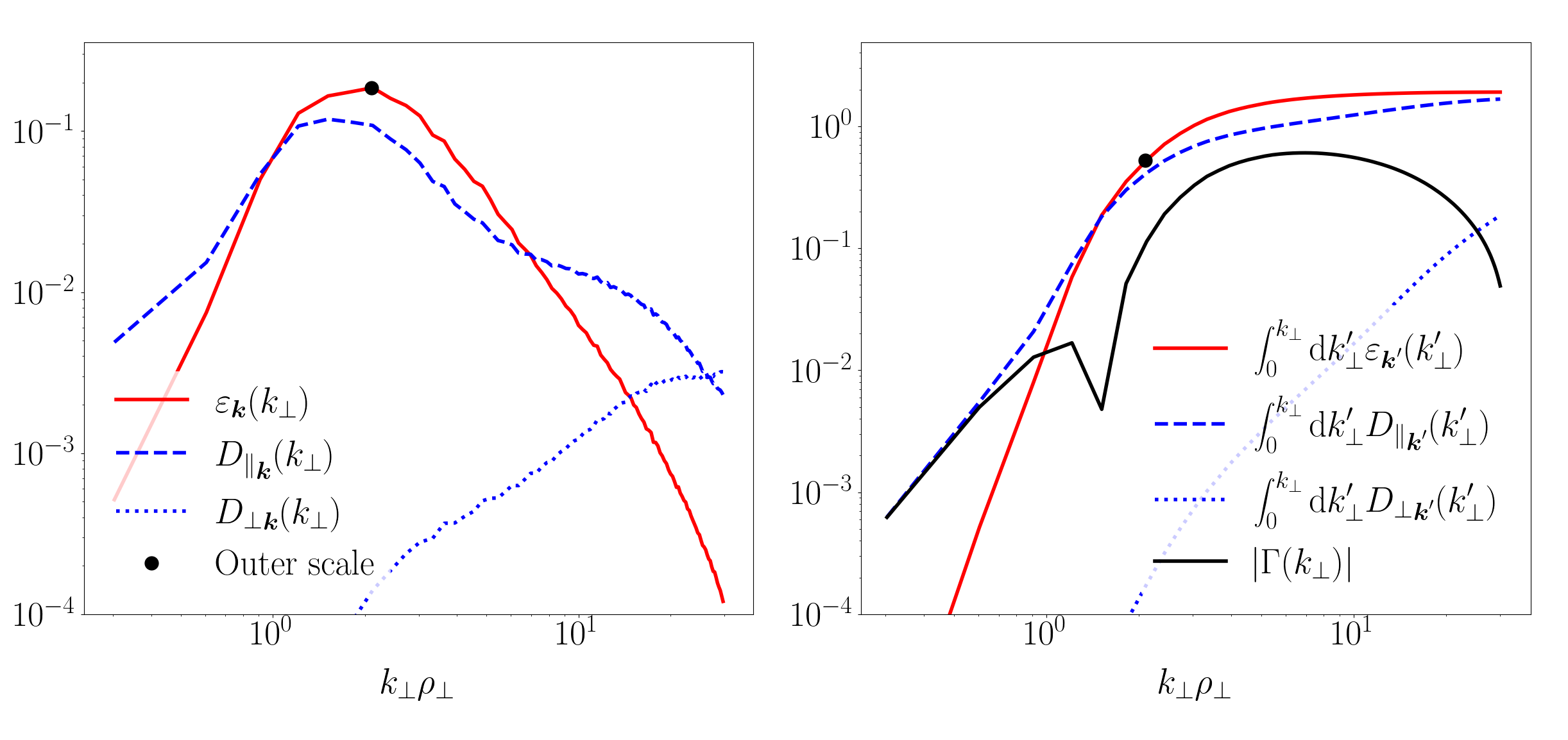
(a)	(b)

Figure 5: (a) 1D perpendicular spectra of the energy injection eq. 33 (solid red), parallel dissipation eq. 34 (dashed blue) and perpendicular dissipation eq. 35 (dotted blue), normalised to $(\rho_{e}/L_{T})^{2}\nu_{ei}/2$. The location of the outer scale is shown by the black dot. The rate of parallel dissipation is significant at the largest scales, while perpendicular dissipation takes over at the smallest scales. (b) The cumulative perpendicular wavenumber integrals of the quantities plotted in (a), as well as the nonlinear energy flux eq. 36 (solid black line). The latter is approximately constant in the inertial range, displaying only an order-unity variation, due to the finite simulation domain.

Plotting the injection and dissipation spectra eq. 33-eq. 35 in fig. 5(a) allows us to make a series of important observations. The first, and unsurprising, one is that the perpendicular dissipation due to hyperviscosity is dominant only at the very smallest scales, where ${D_{\perp}}_{{\boldsymbol{k}}}$ peaks. This confirms the assertion made in section 4.1 that it can be viewed as a sink of energy that exists at higher perpendicular wavenumbers and has no significant effect on the dynamics. The outer scale — at which energy is primarily injected into the turbulence and which we define as corresponding to the perpendicular wavenumber where the maximum of eq. 33 is achieved — appears to be independent of hyperviscosity, being localised on much larger scales, where ${D_{\perp}}_{{\boldsymbol{k}}}$ is negligible. The arguments of section 3.2 leading to the heat-flux scaling eq. 6 relied on the scale invariance of the drift-kinetic system, which, as we have discussed previously, is broken by the introduction of hypervisocisty. The fact that the energy injection is both independent of hypervisocisty and localised at the largest scales supports the prediction of eq. 6 that the heat flux should be determined by the inviscid dynamics at scales where scale-invariant drift kinetics is valid.

Considering scales that are larger than the injection scale, it is clear from fig. 5 that the parallel dissipation ${D_{\parallel}}_{{\boldsymbol{k}}}$ is dominant there, peaking on scales comparable to the outer scale. This is because the existence of the collisional sETG instability depends intrinsically on the presence of thermal conduction (see section 3.3), which is a dissipative effect. Indeed, the maximum growth rate eq. 26 occurs where the rates of thermal conduction and energy injection are comparable, ${\omega_{\parallel}}\sim\omega_{*e}$. Thus, in order to inject energy, the system has to dissipate a finite fraction of it. The energy that survives this dissipation then cascades to small scales through a constant-flux inertial range. This can be seen in fig. 5(b), where we plot the cumulative perpendicular wavenumber integrals of eq. 33, eq. 34, and eq. 35, as well as the nonlinear energy flux, which can be inferred from the difference between injection and dissipation:

$$\Gamma(k_{\perp})=\int_{0}^{k_{\perp}}\mathrm{d}k_{\perp}^{\prime}\>\left[\varepsilon_{{\boldsymbol{k}}^{\prime}}(k_{\perp}^{\prime})-{D_{\parallel}}_{{\boldsymbol{k}}^{\prime}}(k_{\perp}^{\prime})-{D_{\perp}}_{{\boldsymbol{k}}^{\prime}}(k_{\perp}^{\prime})\right].$$ (36)

Both the injection and parallel-dissipation rates reach an approximate plateau at scales smaller than the outer scale and are much larger than the nonlinear energy flux, which is approximately constant in the inertial range, displaying an order-unity variation due to the finite width of the latter in our numerical simulations. The remainder of section 5 is devoted to characterising the dynamics in the inertial range in order to explain how the system organises itself to maintain a constant-flux cascade to small scales despite the presence of significant (parallel) dissipation.

5.2 Constant flux and critical balance in the inertial range

The results of the previous section suggest that our fully developed electrostatic turbulence organises itself into a state wherein there is a local cascade of the free energy eq. 28 that carries the injected power from the outer scale, through an inertial range, to the (perpendicular) dissipation scale. This injected power is the (order-unity) fraction of $\varepsilon$ that survives the parallel dissipation at larger scales, viz., $\varepsilon-D_{\parallel}$, which, for brevity, we shall call $\varepsilon$ in the scaling arguments that follow.

The only nonlinearity in our equations is the advection of the temperature fluctuations by the fluctuating ${\boldsymbol{E}}\times{\boldsymbol{B}}$ flows in eq. 16. Therefore, we take the nonlinear cascade time to be the nonlinear ${\boldsymbol{E}}\times{\boldsymbol{B}}$ advection time:

$$t_{\text{nl}}^{-1}\sim k_{\perp}v_{E}\sim\rho_{e}v_{{\rm th}e}k_{\perp}^{2}\bar{\varphi}\sim\Omega_{e}(k_{\perp}\rho_{e})^{2}\bar{\varphi}.$$ (37)

Here and in what follows, $\bar{\varphi}$ refers to the characteristic amplitude of the electrostatic potential at the scale $k_{\perp}^{-1}$. Formally, $\bar{\varphi}$ can be defined by

$$\bar{\varphi}^{2}=\int_{k_{\perp}}^{\infty}\mathrm{d}k_{\perp}^{\prime}\>E_{\perp}^{\varphi}(k_{\perp}^{\prime}),\quad E_{\perp}^{\varphi}(k_{\perp})\equiv\int_{-\infty}^{\infty}\mathrm{d}k_{\parallel}\>2\pi k_{\perp}\left<|\varphi_{{\boldsymbol{k}}}|^{2}\right>,$$ (38)

where $E_{\perp}^{\varphi}(k_{\perp})$ is the 1D perpendicular spectrum of $\varphi$, $\varphi_{{\boldsymbol{k}}}$ is the spatial Fourier transform of the potential, and the angle brackets denote an ensemble average. The corresponding quantities for the temperature perturbations, $\delta\bar{T}_{e}$, $E_{\perp}^{T}(k_{\perp})$, and ${\delta T_{e}}_{{\boldsymbol{k}}}$, are defined analogously.

Assuming that any possible anisotropy in the perpendicular plane can be neglected (an assumption that will be verified in section 5.5), a Kolmogorov-style constant-flux argument leads to a scaling of the amplitudes in the inertial range:

$$t_{\text{nl}}^{-1}\frac{\delta\bar{T}_{e}^{2}}{T_{0e}^{2}}\sim\varepsilon=\text{const}\quad\Rightarrow\quad\bar{\varphi}\frac{\delta\bar{T}_{e}^{2}}{T_{0e}^{2}}\sim\frac{\varepsilon}{\Omega_{e}}(k_{\perp}\rho_{e})^{-2}.$$ (39)

We are using the $\delta T_{e}/T_{0e}$ part of the free energy eq. 28 because, as we noted earlier, in eq. 15-eq. 16, $\delta T_{e}/T_{0e}$ is the only field that is advected nonlinearly whereas $\varphi$ is ‘sourced’ by the temperature perturbations through the second term on the left-hand side of eq. 15.

To estimate the size of the electrostatic potential, we therefore balance the two terms in eq. 15, yielding

$$\bar{\varphi}\sim\frac{{\omega_{\parallel}}}{\omega}\frac{\bar{\delta T_{e}}}{T_{0e}},$$ (40)

which should hold at every scale. This implies that the potential and temperature perturbations will be comparable in magnitude and have the same wavenumber scaling throughout the inertial range if we posit, scale by scale, that

$$t_{\text{nl}}^{-1}\sim\omega\sim{\omega_{\parallel}}.$$ (41)

This is the conjecture of critical balance, whereby the characteristic time associated with parallel dynamics along the field lines is assumed comparable to the nonlinear advection rate $t_{\text{nl}}^{-1}$ at each perpendicular scale $k_{\perp}^{-1}$, as in Barnes et al. (2011) and Adkins et al. (2022). The original rationale for this conjecture comes from the causality argument proposed in the context of MHD turbulence (Goldreich & Sridhar, 1995; Boldyrev, 2005; Schekochihin, 2022): two points along a field line can only remain correlated with one another if information can propagate between them faster than they are decorrelated by the (perpendicular) nonlinearity; in MHD, this information is carried by Alfvén waves (similarly, it can be carried by other waves in different plasma and hydro-dynamical systems: see Cho & Lazarian 2004; Nazarenko & Schekochihin 2011; Adkins et al. 2022). In our system, the parallel dynamics are dissipative, with the relevant timescale being set by the parallel conduction rate ${\omega_{\parallel}}$. Since there is no mechanism to preserve the parallel coherence of structures created by perpendicular mechanisms (via injection due to the sETG instability, or nonlinear cascade), one expects them to break up in the parallel direction to as fine scales as the system will allow, i.e., structures for which ${\omega_{\parallel}}\ll t_{\text{nl}}^{-1}$ should be immediately decorrelated by the nonlinearity and broken up into shorter pieces in the parallel direction. The limiting factor for this parallel refinement is that if structures reach parallel scales such that ${\omega_{\parallel}}\gg t_{\text{nl}}^{-1}$, they are wiped out by heat conduction. As a result, the “dissipation ridge” (the line of critical balance) ${\omega_{\parallel}}\sim t_{\text{nl}}^{-1}$ will form a natural locus for turbulent structures. This is a version of critical balance that is appropriate for a system where parallel dissipation is present everywhere [which may also be true for collisionless plasmas, where ${\omega_{\parallel}}$ is instead the Landau (1946) damping rate]. In section 5.1, we saw that the actual amount of parallel dissipation that happens in the inertial range is small — free energy chooses to stay just shy of the dissipation region (${\omega_{\parallel}}>t_{\text{nl}}^{-1}$) and instead cascade, at an approximately constant rate, along the dissipation ridge (${\omega_{\parallel}}\sim t_{\text{nl}}^{-1}$).

Combining eq. 39, eq. 40 and eq. 41, we find the following scaling of the amplitudes in the inertial range

$$\bar{\varphi}\sim\frac{\bar{\delta T_{e}}}{T_{0e}}\sim\left(\frac{\varepsilon}{\Omega_{e}}\right)^{1/3}(k_{\perp}\rho_{e})^{-2/3}.$$ (42)

Then, recalling eq. 38, the 1D perpendicular energy spectra in the inertial range are:

$$E_{\perp}^{\varphi}(k_{\perp})\sim E_{\perp}^{T}(k_{\perp})\sim\frac{\bar{\varphi}^{2}}{k_{\perp}}\propto k_{\perp}^{-7/3}.$$ (43)

Using eq. 37 and eq. 42, the critical balance eq. 41 translates into the following relationship between parallel and perpendicular scales in the inertial range:

$$k_{\parallel}\lambda_{ei}\sim\frac{\Omega_{e}^{1/3}\varepsilon^{1/6}}{\nu_{ei}^{1/2}}(k_{\perp}\rho_{e})^{2/3}.$$ (44)

If we define the 1D parallel spectrum

$$E_{\parallel}^{\varphi}(k_{\parallel})\equiv\int_{0}^{\infty}\mathrm{d}k_{\perp}\>2\pi k_{\perp}\left<|\varphi_{{\boldsymbol{k}}}|^{2}\right>,$$ (45)

and the corresponding temperature spectrum $E_{\parallel}^{T}(k_{\parallel})$ analogously, eq. 44 and eq. 42 imply the following inertial-range scaling of amplitudes with parallel wavenumbers:

$$\bar{\varphi}\propto k_{\parallel}^{-1}\quad\Rightarrow\quad E_{\parallel}^{\varphi}(k_{\parallel})\sim E_{\parallel}^{T}(k_{\parallel})\sim\frac{\bar{\varphi}^{2}}{k_{\parallel}}\propto k_{\parallel}^{-3}.$$ (46)

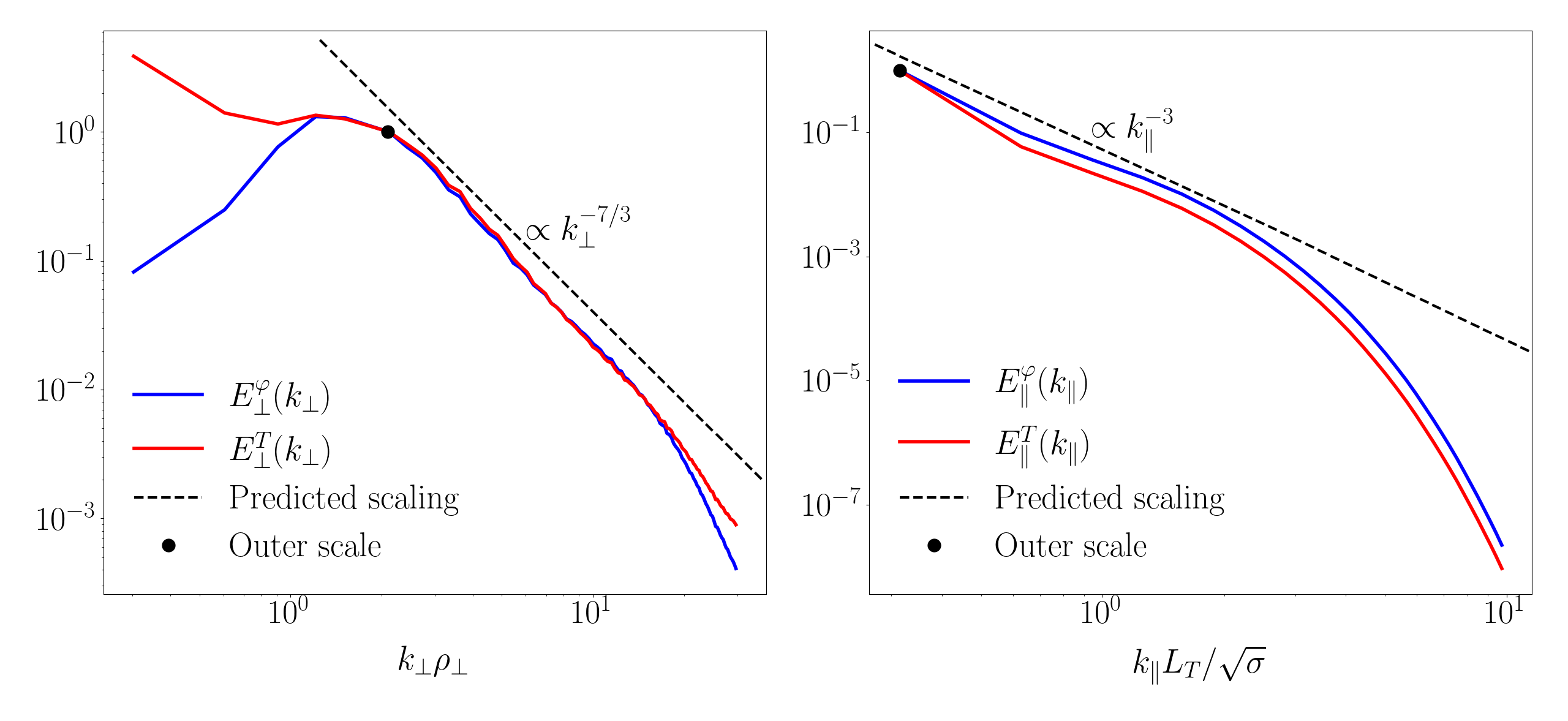
(a)	(b)

Figure 6: The 1D (a) perpendicular eq. 38 and (b) parallel eq. 45 spectra, normalised to their value at the outer scale. The spectra of the electrostatic potential are plotted in blue, those of the temperature perturbations are in red. The predicted inertial-range scalings eq. 43 and eq. 46 are shown by the dashed black lines. The location of the outer scale (see section 5.3) is indicated by the black dot. In (a), this is calculated from the maximum of eq. 33, while in (b), it is calculated from the maximum of the 1D parallel spectrum of the energy injection, defined analogously to eq. 33.

These simple scaling arguments are vindicated by simulation data. The 1D spectra eq. 38 and eq. 45 for both $\varphi$ and $\delta T_{e}$ are plotted in fig. 6. They follow quite well the predicted scalings eq. 43 and eq. 46, respectively, below the outer scale and up to the wavenumbers at which the spectra begin to steepen due to perpendicular dissipation.

We shall return to these inertial-range scalings in section 5.4, where we will study the full 2D spectra of the turbulence and provide further support for the argument that the cascade follows the dissipation ridge (the line of critical balance), but first let us demonstrate how the simple scaling theory developed above allows one to recover — now on physically motivated dynamical grounds — the scaling of the heat flux eq. 6 that was previously inferred from a formal scaling symmetry of our equations.

5.3 Outer scale and scaling of heat flux

From eq. 26, we know that, for a given $k_{y}$, the most unstable collisional sETG modes satisfy

$${\omega_{\parallel}}\sim\omega_{*e}\sim k_{y}\rho_{e}\frac{v_{{\rm th}e}}{L_{T}},$$ (47)

and thus grow at a rate $\sim\omega_{*e}\propto k_{y}$. This means that the linear instability will be overwhelmed by nonlinear interactions in the inertial range, because their characteristic rate increases more quickly with perpendicular wavenumber: from eq. 37 and eq. 42,

$$t_{\text{nl}}^{-1}\sim\Omega_{e}\left(\frac{\varepsilon}{\Omega_{e}}\right)^{1/3}(k_{\perp}\rho_{e})^{4/3}.$$ (48)

The outer scale is then the scale at which these two rates are comparable: balancing eq. 48 and eq. 47, we get

$$\Omega_{e}(k_{\perp}^{o}\rho_{e})^{2}\bar{\varphi}^{o}\sim\omega_{\parallel}^{o}\sim\omega_{*e}\quad\Rightarrow\quad\bar{\varphi}^{o}\sim(k_{\perp}^{o}L_{T})^{-1},\quad k_{y}^{o}\rho_{e}\sim(k_{\parallel}^{o})^{2}L_{T}\lambda_{ei},$$ (49)

where the superscript ‘$o$’ refers to outer-scale quantities. Thus, we have two relationships between $k_{\perp}^{o}$, $\bar{\varphi}^{o}$ and $k_{\parallel}^{o}$, but in order to determine the outer-scale quantities uniquely, we need a third constraint. Given that our system eq. 15-eq. 16 is scale invariant, there is no special (microscopic) perpendicular scale that can be used to fix $k_{y}^{o}$. Then, assuming that the heat flux is independent of the perpendicular system size, the only remaining physically meaningful length scale that can set the outer scale is the parallel system size $L_{\parallel}$. The same should be true for more general systems described by electrostatic drift kinetics, as the scaling eq. 6 would suggest and as we shall discuss shortly.

Assuming, then, that the outer scale is indeed set by the parallel system size, we find from eq. 49:

$$k_{\parallel}^{o}L_{\parallel}\sim 1\quad\Rightarrow\quad\left(\frac{L_{T}}{\rho_{\perp}}\right)\bar{\varphi}^{o}\sim\left(k_{\perp}^{o}\rho_{\perp}\right)^{-1},\quad k_{\perp}^{o}\rho_{\perp}\sim\left(\frac{L_{T}}{L_{\parallel}\sqrt{\sigma}}\right)^{2},$$ (50)

where $\rho_{\perp}$ and $\sigma$ are defined in eq. 18, and the magnitude of $\sigma$ only matters for the purposes of normalising amplitudes and wavenumbers in plots. Figure 7 shows that these theoretical predictions agree very well with the data from the scan in $L_{\parallel}/L_{T}$ that was presented in section 4.2.

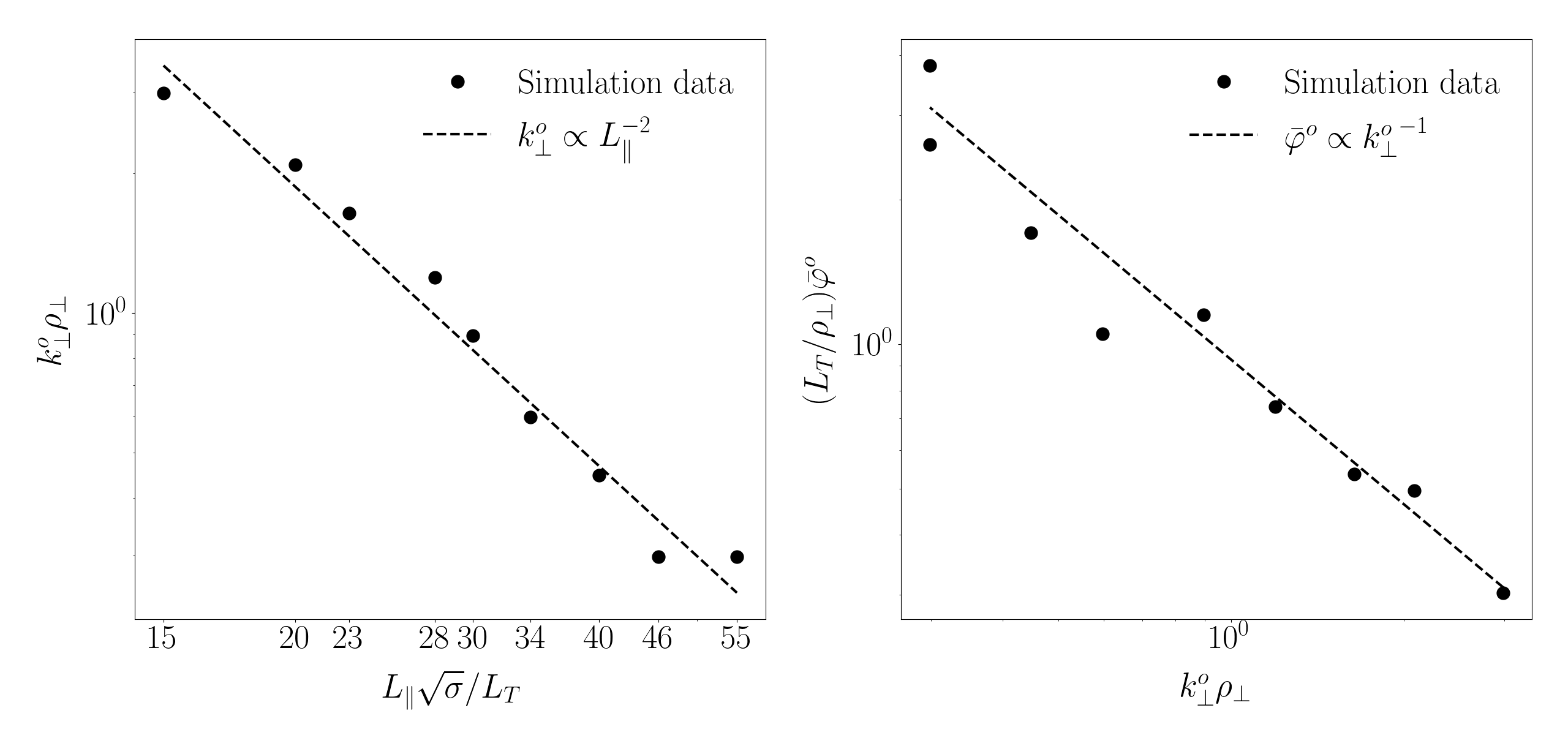
(a)	(b)

Figure 7: (a) The scaling of the perpendicular outer scale $k_{\perp}^{o}$ [defined as the peak wavenumber of the energy injection eq. 33] with $L_{\parallel}/L_{T}$. (b) The scaling of the amplitude of the electrostatic potential $\bar{\varphi}^{o}$ [defined as the amplitude of $\varphi$ at $k_{\perp}=k_{\perp}^{o}$, via eq. 38] with the perpendicular outer scale. The black points are the simulation data, while the theoretical predictions eq. 50 are shown by the black dashed lines. A logarithmic fit to the data gives the slopes of -1.99 and -0.95 in (a) and (b), respectively.

Let us now estimate the energy flux that is injected by the collisional sETG instability at the outer scale eq. 50: using its definition eq. 30, and ignoring any possibility of a non-order-unity contribution from phase factors, we have, from eq. 40, eq. 49 and eq. 50,

$$\varepsilon\sim\omega_{*e}^{o}\bar{\varphi}^{o}\frac{\delta\bar{T}_{e}^{o}}{T_{0e}}\sim\frac{v_{{\rm th}e}\rho_{e}^{2}}{L_{T}^{3}}(k_{\perp}^{o}\rho_{e})^{-1}\sim\frac{v_{{\rm th}e}\rho_{e}^{2}L_{\parallel}^{2}}{\lambda_{ei}L_{T}^{4}}.$$ (51)

Recalling eq. 1, the combination of eq. 51 and eq. 49 yields the following expression for the turbulent heat flux:

$$Q_{e}\sim n_{0e}T_{0e}\varepsilon L_{T}\sim Q_{\text{gB}e}\frac{L_{T}}{\lambda_{ei}}\left(\frac{L_{\parallel}}{L_{T}}\right)^{2}\propto\frac{L_{\parallel}^{2}}{L_{T}^{3}},$$ (52)

where once again $Q_{\text{gB}e}=n_{0e}T_{0e}v_{{\rm th}e}(\rho_{e}/L_{T})^{2}$ is the “gyro-Bohm” flux. Unsurprisingly, this reproduces the scaling with $L_{\parallel}$ given by eq. 6 for $\alpha=2$ [cf., also, eq. 7 for $G=L_{T}/\lambda_{ei}$]. Note that, apart from the inevitable dimensional factors, the $L_{\parallel}$ scaling determines (the nontrivial part of) the dependence of the turbulent heat flux on the temperature gradient, as we anticipated following eq. 6. The fact that our equations eq. 15 and eq. 16 are invariant under the same transformation as drift kinetics eq. 3 means that obtaining this scaling was, in a sense, a foregone conclusion. That being said, in arriving at eq. 52 via this alternative route, we have been able to elucidate the dynamical origin of this scaling, viz., that it is consistent with a critically balanced, constant-flux nonlinear cascade of free energy to small perpendicular scales. This conclusion is not exclusive to the collisional model considered in this paper. Starting from eq. 37, one can construct an entirely analogous theory for the turbulence driven by the collisionless sETG instability, obtaining a result equivalent to eq. 52, which reproduces the scaling eq. 6, this time for $\alpha=1$ (see Adkins et al., 2022).

Let us discuss the significance of our finding that the outer scale is fixed by the assumption that $k_{\parallel}^{o}L_{\parallel}\sim 1$. Such a choice goes back to the work by Barnes et al. (2011), who conjectured, and numerically verified, that the outer scale of electrostatic, gyrokinetic ITG turbulence in tokamak geometry was set by the connection length $L_{\parallel}\sim qR$. While in their case, like ours, this was the only scale that could be reasonably viewed as the characteristic system size (the spatial inhomogeneity of the magnetic equilibrium), there was also another, seemingly more physically intuitive, justification available for its role in determining the large-scale cutoff for the ITG turbulence: one could assume that any turbulent structures correlated on parallel scales longer than the connection length would be damped in the stable (“good-curvature”) region on the inboard side of the tokamak. Thus, one could believe that the operative reason for the significance of $L_{\parallel}\sim qR$ was the presence of large-scale dissipation, rather than, as we have now concluded, just the breaking of scale invariance — in our case, by the finiteness of a periodic box in the parallel direction. A practical implication of this conclusion for more realistic systems appears to be that any long-scale parallel inhomogeneity should be sufficient to set $k_{\parallel}^{o}$, without the need for it to be tied to an energy sink — this could matter for the analysis of turbulence in, e.g., edge plasmas (Parisi et al., 2020, 2022) or in stellarators (Roberg-Clark et al., 2022), where magnetic fields have parallel structure on scales shorter than the connection length.

5.4 Two-dimensional spectra

To provide a more detailed description of the critically balanced cascade (and to provide more evidence that it is indeed a critically balanced cascade), it is interesting to consider the 2D spectra:

$$E^{\varphi}_{2\text{D}}(k_{\perp},k_{\parallel}) =2\pi k_{\perp}\left<|\varphi_{{\boldsymbol{k}}}|^{2}\right>,$$ (53)

$$E^{T}_{2\text{D}}(k_{\perp},k_{\parallel}) =2\pi k_{\perp}\left<|{\delta T_{e}}_{{\boldsymbol{k}}}/T_{0e}|^{2}\right>.$$ (54)

Unlike in section 5.2, we can no longer assume that $E^{\varphi}_{2\text{D}}\sim E^{T}_{2\text{D}}$; this was true only for the “integrated” 1D spectra dominated by the wavenumbers where the critical-balance conjecture eq. 41 was assumed satisfied, and the two fields thus had the same scaling eq. 40 for $\omega\sim\omega_{\parallel}$. With this in mind, we will first consider the spectrum of the temperature perturbations, from which the spectrum of the potential perturbations can then be inferred via eq. 40.

We consider two wavenumber regions, above and below the “critical-balance line” eq. 44:

$$E_{2\text{D}}^{T}(k_{\perp},k_{\parallel})\sim\left\{\begin{array}[]{ll}\displaystyle k_{\parallel}^{-a}k_{\perp}^{b},&\displaystyle k_{\parallel}\gtrsim k_{\perp}^{2/3},\\[11.38109pt] \displaystyle k_{\perp}^{-c}k_{\parallel}^{d},&\displaystyle k_{\parallel}\lesssim k_{\perp}^{2/3},\end{array}\right.$$ (57)

where $a$, $b$, $c$, and $d$ are positive constants to be determined. Here, and in what follows, whenever our expressions appear to be dimensionally incorrect, this is because we have implicitly chosen to normalise our wavenumbers to the outer scale $k_{\parallel}/k_{\parallel}^{o}\rightarrow k_{\parallel}$, $k_{\perp}/k_{\perp}^{o}\rightarrow k_{\perp}$ so as to reduce notational clutter. To determine the scaling exponents, we follow the general scheme, which, for MHD turbulence, was laid out by Schekochihin (2022) (see his appendix C).

Evidently, the scalings in the two regions in eq. 57 must match along the boundary $k_{\parallel}\sim k_{\perp}^{2/3}$, giving

$$a+d=\frac{3}{2}(b+c).$$ (58)

If $a>1$ and $d>-1$, $k_{\parallel}\sim k_{\perp}^{2/3}$ will be the energy-containing parallel wavenumber at a given $k_{\perp}$. The 1D perpendicular spectrum is, therefore,

$$E_{\perp}^{T}(k_{\perp})=\int\mathrm{d}k_{\parallel}\>E_{2\text{D}}^{T}(k_{\perp},k_{\parallel})\sim\int_{0}^{k_{\perp}^{2/3}}\mathrm{d}k_{\parallel}\>k_{\perp}^{-c}k_{\parallel}^{d}\sim k_{\perp}^{-c+2(1+d)/3}.$$ (59)

This must match the scaling eq. 43 of the 1D perpendicular spectrum derived from the constant-flux conjecture, implying that

$$c=\frac{2}{3}(1+d)+\frac{7}{3}.$$ (60)

Two further constraints follow from imposing boundary conditions as $k_{\parallel}$ or $k_{\perp}\rightarrow 0$ at constant $k_{\perp}$ or $k_{\parallel}$, respectively. The scaling of the spectrum as $k_{\perp}\rightarrow 0$ (in the region $k_{\parallel}\gg k_{\perp}^{2/3}$) can be determined purely kinematically: the low-$k_{\perp}$ asymptotic behaviour of a homogenous 2D-isotropic field must be $k_{\perp}^{3}$, implying that

$$b=3.$$ (61)

This is a fairly standard result (see, e.g., appendix A of Schekochihin et al., 2016). Finally, the scaling as $k_{\parallel}\rightarrow 0$ (in the region $k_{\parallel}\ll k_{\perp}^{2/3}$) follows from causality. Indeed, in section 5.2, we argued that fluctuations become decorrelated for $\omega_{\parallel}\lesssim t_{\text{nl}}^{-1}$ because they cannot communicate across parallel distances $\sim k_{\parallel}^{-1}$, but such $k_{\parallel}$ are also too small for the fluctuations to be erased by thermal conduction. Therefore, the parallel spectrum at $k_{\parallel}\ll k_{\perp}^{2/3}$ must be the spectrum of a 1D white noise:

$$d=0.$$ (62)

Combining eq. 61 and eq. 62 with eq. 58 and eq. 60, we find

$$a=9,\quad c=3.$$ (63)

This gives us the following scalings for the 2D spectrum of the temperature perturbations:

$$E_{2\text{D}}^{T}(k_{\perp},k_{\parallel})\sim\left\{\begin{array}[]{ll}\displaystyle k_{\parallel}^{-9}k_{\perp}^{3},&\displaystyle k_{\parallel}\gtrsim k_{\perp}^{2/3},\\[11.38109pt] \displaystyle k_{\perp}^{-3}k_{\parallel}^{0},&\displaystyle k_{\parallel}\lesssim k_{\perp}^{2/3}.\end{array}\right.$$ (66)

Turning now to the 2D spectrum of the potential perturbations, analogously to eq. 57, the conditions eq. 58 and eq. 60 are unmodified — the spectrum must still be continuous along $k_{\parallel}\sim k_{\perp}^{2/3}$, and match the scaling of the 1D perpendicular spectrum that follows from the constant-flux conjecture, which is the same for both the potential and temperature perturbations. Similarly, the scaling of the spectrum as $k_{\perp}\rightarrow 0$ (in the region $k_{\parallel}\gtrsim k_{\perp}^{2/3}$) will once again be $k_{\perp}^{3}$ by the same kinematic argument, implying eq. 61. From eq. 58 and eq. 60, we again have $a=9$. However, the causality argument that led to the white-noise scaling eq. 62 at $k_{\parallel}\lesssim k_{\perp}^{2/3}$ now no longer holds, because $\varphi$ is not directly decorrelated by the nonlinearity. Instead, it inherits its scaling from $\delta T_{e}/T_{0e}$ via the balance eq. 40, viz.,

$$E_{2\text{D}}^{\varphi}\sim\frac{\omega_{\parallel}^{2}}{\omega^{2}}E_{2\text{D}}^{T}\sim\frac{k_{\parallel}^{4}k_{\perp}^{-3}}{\omega^{2}},$$ (67)

where we have used $\omega_{\parallel}\propto k_{\parallel}^{2}$ and the second expression in eq. 66. Now, in the region $k_{\parallel}\lesssim k_{\perp}^{2/3}$, we expect thermal conductivity in the temperature equation to be subdominant to the nonlinear rate, and so estimating $\omega\sim t_{\text{nl}}^{-1}\propto k_{\perp}^{4/3}$ in eq. 67, we find that

$$d=4,\quad c=\frac{17}{3}.$$ (68)

This gives us the following scalings of the 2D spectrum of the potential fluctuations:

$$E_{2\text{D}}^{\varphi}(k_{\perp},k_{\parallel})\sim\left\{\begin{array}[]{ll}\displaystyle k_{\parallel}^{-9}k_{\perp}^{3},&\displaystyle k_{\parallel}\gtrsim k_{\perp}^{2/3},\\[11.38109pt] \displaystyle k_{\perp}^{-17/3}k_{\parallel}^{4},&\displaystyle k_{\parallel}\lesssim k_{\perp}^{2/3}.\end{array}\right.$$ (71)

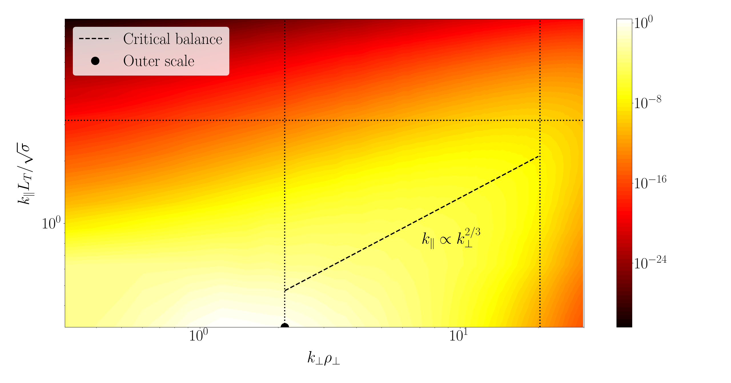
Figure 8: A contour plot of the logarithm of the 2D spectrum eq. 54 of the temperature perturbations in the $(k_{\perp},k_{\parallel})$ plane, normalised to its value at the outer scale. The line of critical balance is shown as the dashed black line, while the outer scale is shown by the black dot. The horizontal dotted line shows the upper bound on the parallel-wavenumber cuts plotted in the right panels of fig. 9. Similarly, the vertical dotted lines show the lower and upper bounds on the perpendicular-wavenumber cuts plotted in the right panels of fig. 10.

The full 2D spectrum of the temperature perturbations is plotted in fig. 8. The organisation of the system about the critical-balance line is manifest here. Cuts of the 2D spectra eq. 53 and eq. 54 at constant $k_{\parallel}$ and $k_{\perp}$ are shown in figures 9 and 10, respectively, for both potential and temperature perturbations, showing good agreement with the theoretical scalings eq. 66 and eq. 71. The white-noise spectra at $k_{\parallel}\lesssim k_{\perp}^{2/3}$, in particular, are another confirmation of the causal nature of the critical balance.

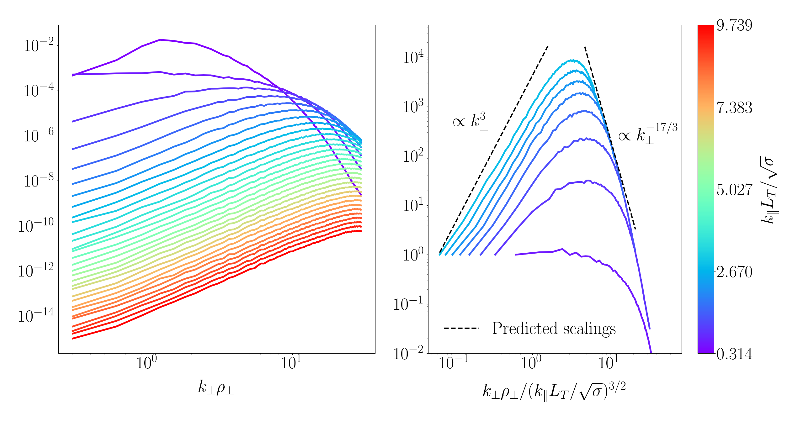
(a) $E_{2\text{D}}^{\varphi}(k_{\perp},k_{\parallel}=\text{const})$

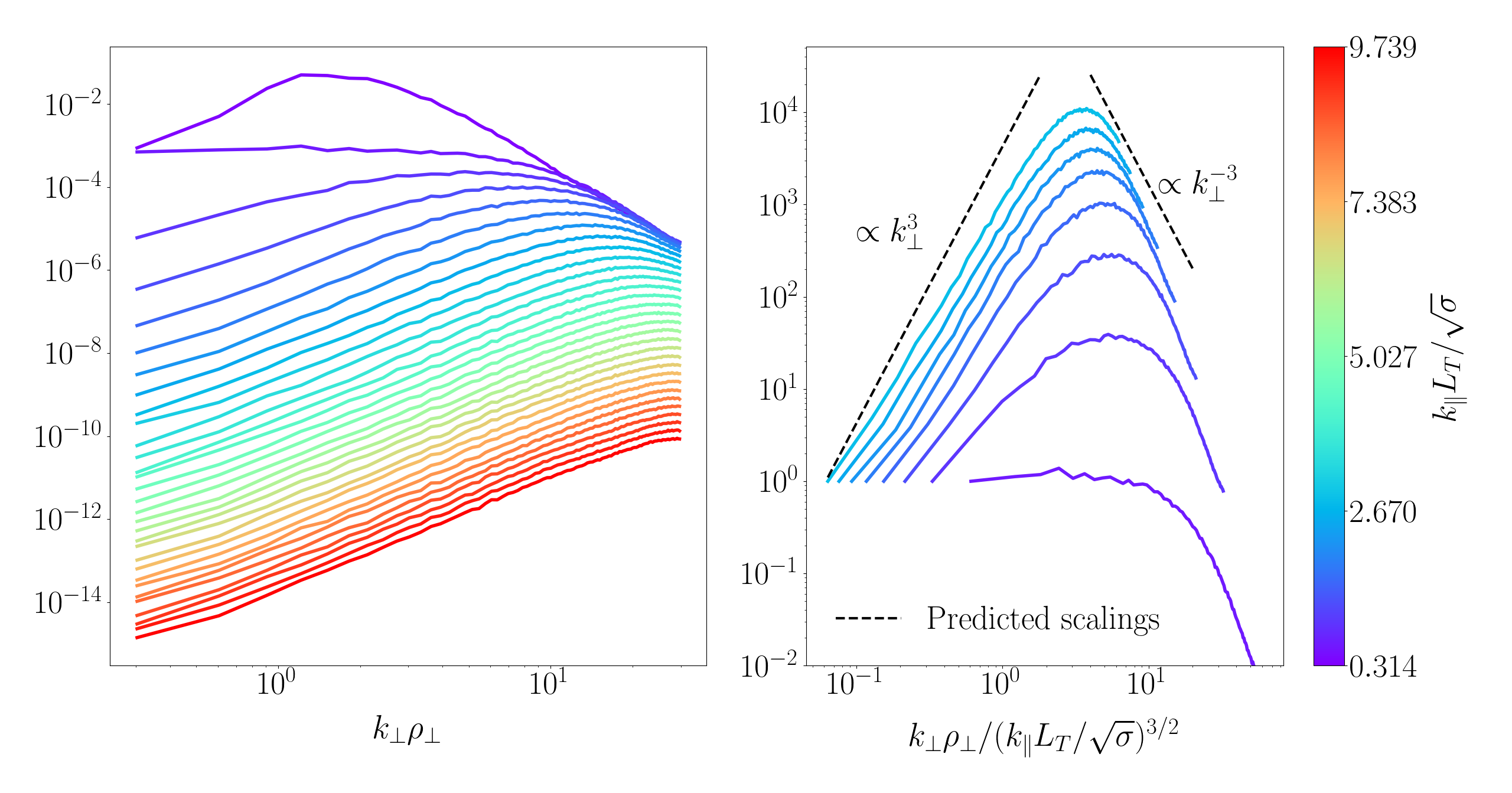
(b) $E_{2\text{D}}^{T}(k_{\perp},k_{\parallel}=\text{const})$

Figure 9: Cuts of the 2D spectra of (a) the electrostatic potential and (b) the temperature perturbations at constant $k_{\parallel}$, normalised to $(\rho_{\perp}/L_{T})^{2}$. The colours indicate the value of $k_{\parallel}L_{T}/\sqrt{\sigma}$ for a given cut. The left panels show the entire spectrum plotted as a function of $k_{\perp}\rho_{\perp}$. The right panels show selected cuts for $k_{\parallel}L_{T}$ within the inertial range, with $k_{\perp}$ rescaled according to the critical-balance relation eq. 44. The black dashed lines show the theoretical scalings eq. 71 and eq. 66 in panels (a) and (b), respectively. The spectra show reasonable agreement with theory at both small and large perpendicular scales, despite the effects of hyperviscosity being present at the smallest scales.

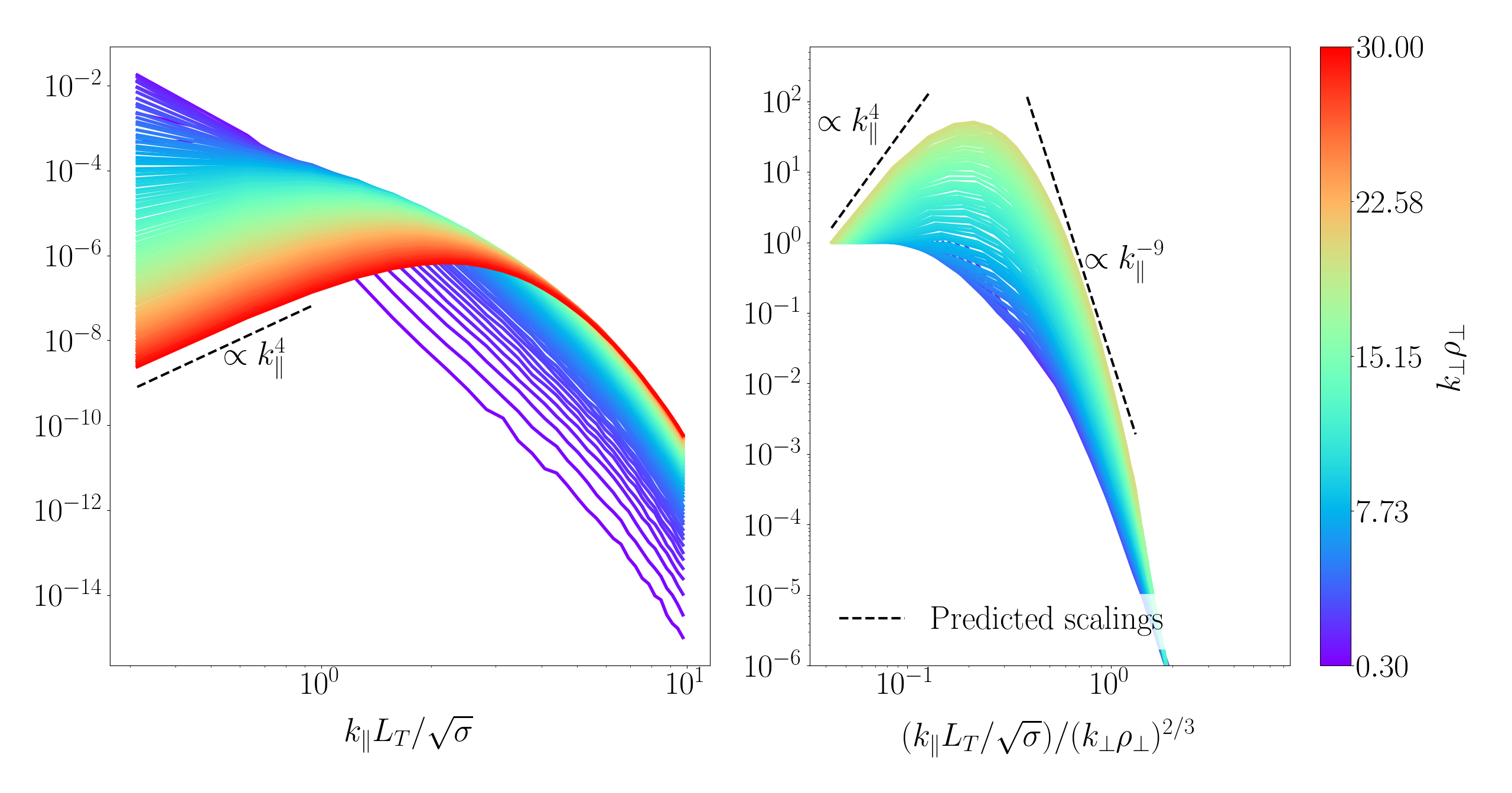
(a) $E_{2\text{D}}^{\varphi}(k_{\perp}=\text{const},k_{\parallel})$

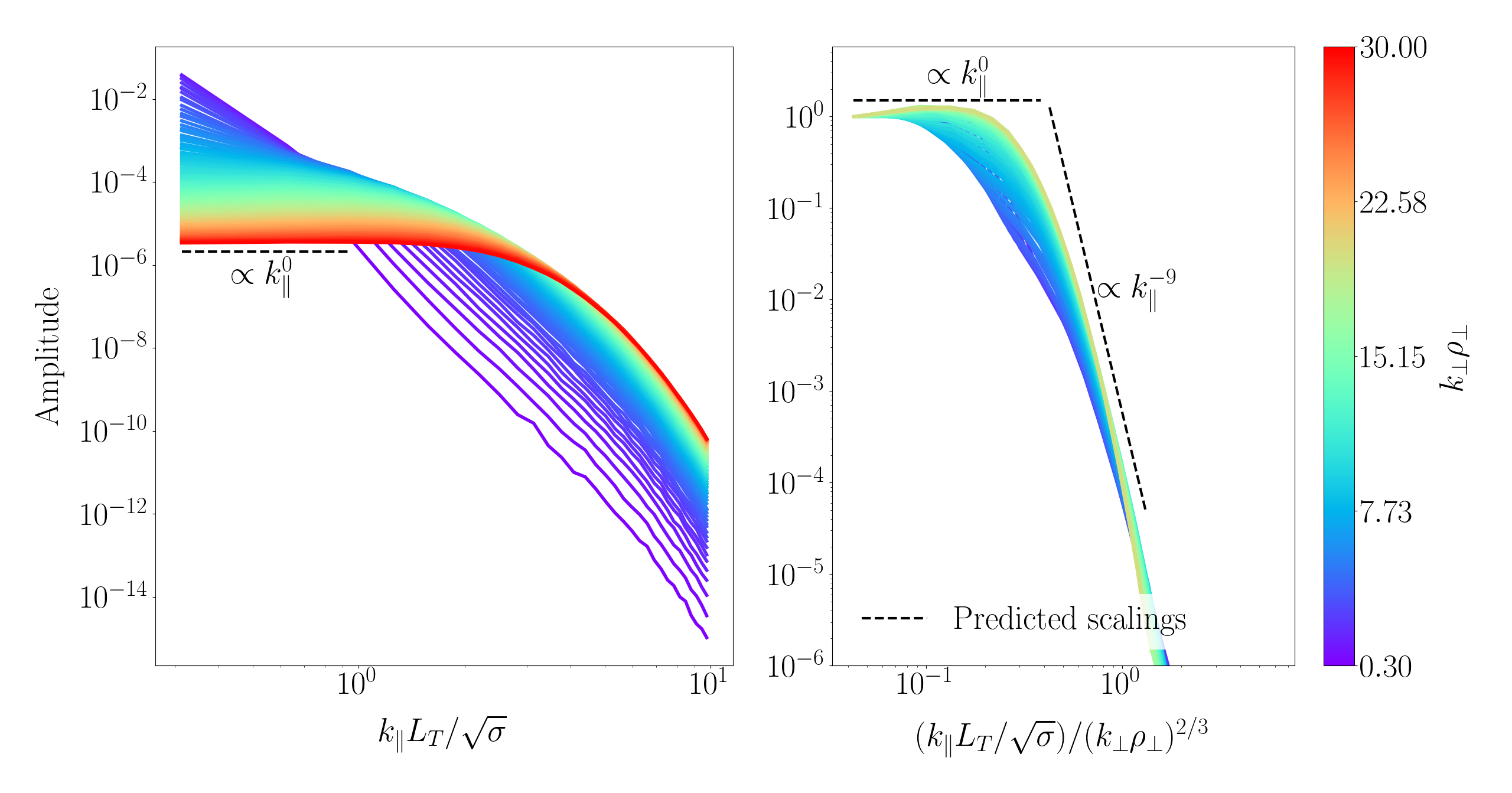
(b) $E_{2\text{D}}^{T}(k_{\perp}=\text{const},k_{\parallel})$

Figure 10: Cuts of the 2D spectra of (a) the electrostatic potential and (b) the temperature perturbations at constant $k_{\perp}$, normalised to $(\rho_{\perp}/L_{T})^{2}$. The colours indicate the value of $k_{\perp}\rho_{\perp}$ for a given cut. The left panels show the entire spectrum plotted as a function of $k_{\parallel}L_{T}$. The right panels show selected cuts of the spectrum for $k_{\perp}\rho_{\perp}$ within the inertial range, with $k_{\parallel}$ rescaled according to the critical-balance relation eq. 44. The black dashed lines show the theoretical scalings eq. 71 and eq. 66 in panels (a) and (b), respectively. There is very good agreement with theory, especially at $k_{\parallel}\lesssim k_{\perp}^{2/3}$, where the scalings extend well beyond the inertial range to higher $k_{\perp}\rho_{\perp}$, as can be seen from the left panels — this is because the causality argument is not sensitive to the precise details of the decorrelation physics.

The extraordinarily steep parallel-wavenumber scaling of the 2D spectra eq. 66 and eq. 71 in the region $k_{\parallel}\gtrsim k_{\perp}^{2/3}$ can also be viewed as further evidence for the version of critical balance proposed following eq. 41. In terms of timescales, this wavenumber constraint corresponds to $\omega_{\parallel}\gtrsim t_{\text{nl}}^{-1}$, and thus to a region of dominant thermal conduction that attempts to erase parallel structure created by the turbulence. The $k_{\parallel}$ scaling in this region proves to be so steep that the free-energy sink due to parallel dissipation is ineffective: the free energy cannot be nonlinearly transferred into this region in an efficient way, and instead cascades towards higher perpendicular wavenumbers along the critical-balance line, eventually encountering perpendicular dissipation, introduced, in our model, through hyperviscosity. Parallel dissipation thus acts not as a sink for the cascade, but instead creates the aforementioned “dissipation ridge”, constraining the cascade of energy in wavenumber space to be along the critical-balance line $k_{\parallel}\sim k_{\perp}^{2/3}$.

One could dismiss this feature as being a peculiarity of our collisional model, given that the dissipative nature of collisional sETG instability eq. 23 is hard-wired into it by construction. However, this picture might not be entirely dissimilar from what is observed in more generic systems of plasma turbulence: e.g., Hatch et al. (2011) observed an overlap of the spatial scales of energy injection and dissipation in electrostatic, ion-scale toroidal gyrokinetic simulations, as did Told et al. (2015) in the context of Alfvénic turbulence. The same behaviour could also be relevant in the context of kinetic ETG-driven turbulence. The growth rate of the collisionless sETG instability is limited by the parallel streaming rate ${\omega_{\parallel}}\sim k_{\parallel}v_{{\rm th}e}$ (see, e.g., Adkins et al., 2022), which is also the rate of Landau damping; viewed in the context of the current discussion, this suggests, perhaps, that Landau damping could play a dissipative role similar to that of the thermal conduction in determining the way in which the system organises itself in order to support a constant-flux cascade of energy to small scales. Then, the rates of either parallel streaming or thermal conduction appearing in the critical balance ${\omega_{\parallel}}\sim\omega\sim t_{\text{nl}}^{-1}$ can also be interpreted as being there because they are the rates of parallel dissipation, rather than of the parallel propagation of information, limiting any further refinement of the parallel scale of the turbulent structures.

5.5 Perpendicular isotropy

Throughout sections 5.2 to 5.4, our theoretical deductions were carried out under the assumption that $k_{x}\sim k_{y}\sim k_{\perp}$. This assumption of perpendicular isotropy is not obviously true and must be tested. Indeed, the maximum sETG growth rate eq. 26 is at $k_{x}=0$, and so the outer-scale energy injection is predominantly into the so-called ‘streamers’: highly anisotropic ($k_{x}\ll k_{y}$) structures that can be identified in real space by their alternating pattern of horizontal bands stretched along the radial ($x$) direction (Cowley et al., 1991). In the context of ITG-driven turbulence, it is often assumed (and usually confirmed numerically) that these streamers are broken apart by zonal flows (see Barnes et al. 2011 and references therein), restoring isotropy at the outer scale; isotropy in the inertial range is then assumed as well. In ETG-driven turbulence, however, the role of zonal flows is less obvious (see, e.g., Dorland et al., 2000; Jenko et al., 2000; Colyer et al., 2017), and the existence of an isotropic state far from guaranteed — indeed, the real-space snapshots shown in fig. 11 suggest that the system is in fact dominated by streamer-like structures on the largest scales, and there is little zonal-flow activity. Qualitatively, this is quite similar to what ETG turbulence has been reported to look like in gyrokinetic simulations (Joiner et al., 2006; Candy et al., 2007; Roach et al., 2009; Guttenfelder & Candy, 2011).

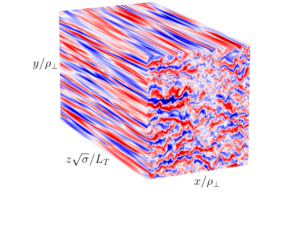
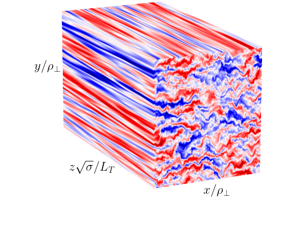
(a) $(L_{T}/\rho_{\perp})\varphi$	(b) $(L_{T}/\rho_{\perp})\delta T_{e}/T_{0e}$

Figure 11: Real-space snapshots of (a) the electrostatic potential and (b) the temperature perturbations from the higher-resolution simulation at $(\rho_{e}/\rho_{\perp})^{2}\nu_{ei}t/2\sigma=3000$ (see table 1). The coordinate axes are as shown, while the red and blue colours correspond to regions of positive and negative fluctuation amplitudes. The turbulence does not appear to be isotropic on the large scales that are visible in these plots (streamers are manifest), but turns out to be isotropic in the inertial range (see fig. 12).

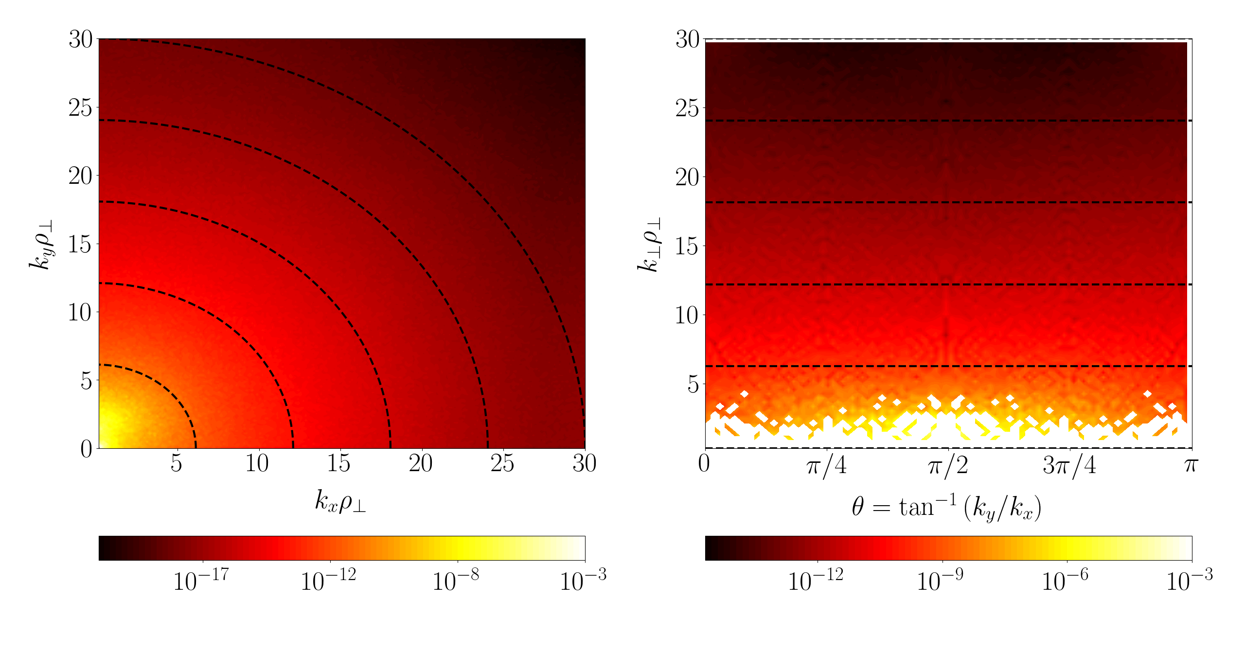
(a) $\log E^{T}(k_{x},k_{y})$	(b) $\log E^{T}(k_{\perp},\theta)$

Figure 12: Contour plots of the two-dimensional spectra of the temperature perturbations, normalised to $(\rho_{\perp}/L_{T})^{2}$: (a) in Cartesian coordinates, with the radial and poloidal wavenumbers plotted on the horizontal and vertical axes, respectively; contours of constant $E^{T}(k_{x},k_{y})$ eq. 72 (black dashed lines) are approximately circular away from the origin, where injection is localised and the presence of streamers is manifested by the spectral power being shifted towards $k_{y}>k_{x}$; (b) in polar coordinates, with $\theta=\tan^{-1}(k_{y}/k_{x})$ and $k_{\perp}\rho_{\perp}$ plotted on the horizontal and vertical axes, respectively; contours of constant $E^{T}(k_{\perp},\theta)$ eq. 73 (black dashed lines) are approximately horizontal far away from $k_{\perp}\rho_{\perp}\lesssim 1$, where injection is localised.

To assess how isotropic the saturated state is, in particular in the inertial range, we plot the two-dimensional spectra

$$E^{T}(k_{x},k_{y}) =\int_{-\infty}^{\infty}\mathrm{d}k_{\parallel}\left<|{\delta T_{e}}_{{\boldsymbol{k}}}/T_{0e}|^{2}\right>,$$ (72)

$$E^{T}(k_{\perp},\theta) =k_{\perp}\int_{-\infty}^{\infty}\mathrm{d}k_{\parallel}\left<|{\delta T_{e}}_{{\boldsymbol{k}}}/T_{0e}|^{2}\right>$$ (73)

in fig. 12. Here and in what follows, $\theta=\tan^{-1}(k_{y}/k_{x})$ is the polar angle in the perpendicular wavenumber plane. In both Cartesian and polar representations, we see that the spectrum is approximately isotropic with respect to the perpendicular wavevectors: at scales sufficiently smaller than the outer scale (viz., in the inertial range) contours of constant $E^{T}$ are either circles, in the case of eq. 72, or horizontal lines, in the case of eq. 73. The spectra of the potential perturbations, defined analogously to eq. 72 and eq. 73, display a similar isotropy. Thus, despite the fact that the largest scales are anisotropic due to the existence of streamers and the lack of vigorous zonal flows to break them apart, isotropy is restored in the inertial range.

The observed lack of zonal-flow activity is linked to the fact that there is nothing on electron scales to give zonal flows privileged status. This makes ETG turbulence quite unlike its ITG cousin on ion scales, where one encounters the modified adiabatic electron response (see, e.g., Hammett et al., 1993; Abel & Cowley, 2013):

$$\frac{\delta n_{i}}{n_{0i}}=\frac{\delta n_{e}}{n_{0e}}=\varphi^{\prime},$$ (74)

where $\varphi^{\prime}$ is the non-zonal component of the (non-dimensionalised) electrostatic potential. Indeed, eq. 74 has been found to be crucial for capturing essential zonal-flow physics (Rogers et al., 2000; Ivanov et al., 2020, 2022). Physically, this can be explained by the fact that eq. 74 reserves a special status for zonal flows, in that it allows there to be non-trivial nonlinear interactions between the zonal flows and $\varphi^{\prime}$ through the electrostatic ${\boldsymbol{E}}\times{\boldsymbol{B}}$ nonlinearity contained in the convective derivative eq. 12 of the density perturbation. However, as we discussed in section 5.2, the adiabatic ion response eq. 14 causes the nonlinearity in the electron continuity equation eq. 15 to vanish identically. Crucially, this means that the system lacks any nonlinearity capable of generating two-dimensional secondary instabilities that are responsible for the generation of zonal flows and destruction of streamer structures (Hasegawa & Mima, 1978; Hasegawa & Wakatani, 1983; Terry & Horton, 1983; Diamond et al., 2005; Ivanov et al., 2020; Zhu et al., 2020). A further consequence of this is that the model system eq. 15-eq. 16 proves to be incapable of generating zonal flows even on longer timescales than those over which the observed isotropisation occurs, unlike what was observed in, e.g., Colyer et al. (2017) and Tirkas et al. (2023).

6 Summary and discussion

We have considered the transport properties of electrostatic, drift-kinetic plasma turbulence, with a particular focus on the connection between its macroscopic transport properties and microscale (inertial-range) dynamics. In the presence of constant perpendicular equilibrium gradients, it has been observed that the equations of electrostatic drift kinetics possess a symmetry associated with their intrinsic scale invariance, in both the collisionless and collisional limits. Under the assumptions of spatial periodicity, stationarity and locality, this symmetry has been shown to imply a particular scaling eq. 6 of the heat flux $Q_{s}$ with the parallel system size $L_{\parallel}$, viz., $Q_{s}\propto L_{\parallel}$ (or $\propto L_{\parallel}^{2}$, in the collisional limit), with the dependence on the equilibrium temperature gradient following from dimensional analysis (in the absence of other equilibrium gradients). This macroscopic transport prediction was then confirmed numerically in an electron-scale, collisional fluid model of electrostatic turbulence driven by the electron-temperature gradient. A critically balanced, constant-flux cascade of energy from some large, outer scale — at which energy is effectively injected by the (collisional) slab ETG instability — to small scales was then shown to be the microscale dynamics consistent with these macroscopic transport properties. This is one of only two extant numerical demonstrations of the existence of such a state in gradient-driven turbulence of this kind — the other being Barnes et al. (2011), for gyrokinetic ITG turbulence.

Two key observations can be made from our results: (i) the effects of dissipation associated with parallel thermal conduction play a key role in determining the saturated state of the turbulence, limiting the cascade of free energy in parallel wavenumbers by clamping it to the “dissipation ridge”, or line of “critical-balance”, in wavenumber space (Landau damping could play an analogous role in the collisionless limit); (ii) the outer scale of the turbulence is determined by the breaking of drift-kinetic scale invariance due to the existence of some long-scale parallel inhomogeneity — in our case, this was the finite size of our periodic box. In more realistic plasma systems like the tokamak, this could be the connection length $L_{\parallel}\sim qR$, or some shorter scale associated with inhomogeneities in the equilibrium magnetic field, such as in the tokamak edge or in stellarators.

These results demonstrate that the details of the (parallel) plasma equilibrium play a central role in determining the microscopic outer scale for the turbulence, and thus the saturated amplitudes to which turbulent fluctuations will grow, which in turn determine the observed macroscopic transport properties. The fact that turbulence in gradient-driven systems appears to behave similarly to those in which energy is injected by explicitly large-scale processes is encouraging from the perspective of theory, as it suggests that existing insights into, and experience of, the latter can be applied to the former, significantly less well-studied case.

Though the implications of drift-kinetic scale invariance were investigated here in a reduced model of ETG-driven turbulence, they nevertheless have implications for more realistic plasma systems due to strong constraints placed on the system by the resultant symmetry of the governing equations. Indeed, it must be stressed that while the physical regimes covered by the reduced model are limited in scope — lacking dynamics associated with, e.g., gradients of the plasma density or equilibrium magnetic field, kinetic effects, etc. — the scaling eq. 6 of the heat flux suffers from no such limitations since it follows directly from the scale invariance of the electrostatic drift-kinetic system of equations. The existence of this scaling, however, is predicated on the adoption of the drift-kinetic limit. Restoring FLR effects by reverting to the (electrostatic) gyrokinetic equation will evidently break the scale invariance, as the scales $k_{\perp}\sim\rho_{s}^{-1}$ will now appear explicitly in the equations through the Bessel functions (see, e.g., Abel et al., 2013). Apart from some interesting exceptions (Parisi et al., 2020, 2022), the general effect of these Bessel functions is to provide a cutoff for instabilities at large perpendicular wavenumbers, restricting the region of instability on the ultraviolet side and providing a sink of energy (dissipation) beyond the wavenumbers where the sETG growth rate peaks. The constant-flux arguments of section 5 assumed that there was sufficient separation between the outer scale and these dissipation regions in order to allow an inertial range to develop at the intermediate scales. Should such a separation exist, the system will effectively be drift-kinetic in the inertial range and, crucially, at the outer scale, where our results will continue to apply, despite the system being fully gyrokinetic. In other words, even if drift-kinetic scale invariance is broken at small scales, the assumption behind eq. 6 is that the transport is set by the outer scale, which is in the drift-kinetic limit, and the relevant breaking of scale-invariance is done by $L_{\parallel}$. This is indeed what we observed in section 5: despite the breaking of scale invariance at small perpendicular scales due to the introduction of hyperviscosity, our simulation results still confirmed the scaling eq. 6 as the well-defined outer scale was still set by $L_{\parallel}$. We acknowledge, however, that the scale separation required for such a state is far from guaranteed: non-zero magnetic shear, for example, can create long-wavelength modes with binormal wavenumbers $k_{y}\rho_{i}\sim 1$ but narrow radial structures near mode-rational surfaces on the scale $k_{x}\rho_{e}\sim 1$ (Hardman et al., 2022, 2023; Parisi et al., 2022). Whether our results are robust to the effects of significant magnetic shear and other forms of equilibrium shaping that can amplify the importance of FLR — and thus undermine the possible separation between FLR effects and a putative outer scale — is a subject for future work.

A key assumption behind the scaling eq. 6 is that the heat flux is able to reach a (statistical) steady state. The existence of such a state, however, is less assured than one might think: indeed, it has been known for some time that nonlinear saturation can fail to occur in simulations of electron-scale, gradient-driven turbulence due to the persistence of large-scale streamer structures in the absence of flow shear or a non-adiabatic ion response (Joiner et al., 2006; Candy et al., 2007; Roach et al., 2009; Guttenfelder & Candy, 2011). In our simple fluid model, we too find that introducing magnetic drifts associated with an inhomogeneous equilibrium magnetic field is sufficient to reproduce this behaviour. In such simulations, the curvature-mediated ETG instability (Horton et al., 1988; Adkins et al., 2022), absent in a straight magnetic field, gives rise to nonlinearly robust, large-scale streamer structures that cause unbounded growth of the heat flux with time. Further details of these simulations can be found in appendix C. This behaviour is consistent with the view that the adiabatic ion response eq. 14 is insufficient to saturate ETG-scale turbulence in the presence of finite magnetic-field gradients (Hammett et al., 1993). It must be stressed that this lack of saturation does not break the drift-kinetic scale invariance eq. 3, which is valid for any constant perpendicular equilibrium gradients, including those of the equilibrium magnetic field — it merely demonstrates that the steady state required to deduce eq. 6 from eq. 3 may not always be achievable in the regime of interest. Indeed, if we had been able to find a case of turbulence driven by the curvature-mediated ETG instability that saturated, we would have expected the scaling eq. 6 for the corresponding heat flux (although not necessarily the same detailed inertial-range structure as for the sETG turbulence that we studied above), but in any event, no such saturated cases have so far presented themselves.

Another limiting assumption of our work was the electrostatic nature of the turbulence. The existence of finite electromagnetic perturbations also formally breaks the (electrostatic) drift-kinetic symmetry observed in section 2 (this is manifest on inspection of the equations of electromagnetic gyrokinetics). However, this does not necessarily imply that the heat-flux scaling eq. 6 can never be realised in systems with finite beta. Indeed, we argued above that this scaling would still hold in the presence of FLR effects if the outer scale of the turbulence remained within the drift-kinetic limit, despite scale invariance being formally broken at the smallest spatial scales. A similar argument is applicable here. If the outer scale lies at scales sufficiently smaller than those on which electromagnetic effects are important (the ‘flux-freezing scale’, determined by the electron inertia in the collisionless limit, or resistivity in the collisional one; see Adkins et al., 2022), then the scaling eq. 6 will continue to hold as, once again, the assumption behind it is that the transport is set by the outer scale located in the electrostatic, drift-kinetic limit, and the relevant breaking of scale invariance is done by $L_{\parallel}$, rather than the flux-freezing scale. For example, Chapman-Oplopoiou et al. (2022) performed nonlinear, electromagnetic simulations of JET-ILW pedestals for $k_{\perp}\rho_{i}\gtrsim 1$, and observed the same scaling of the heat flux with $L_{T}$ as eq. 7 at gradients sufficiently far above the linear threshold. However, if the outer scale lies on scales larger than the flux-freezing scale, i.e., if the turbulence is truly electromagnetic, then the constraints imposed by the scale invariance of electrostatic drift kinetics is lifted. Given that such regimes will likely be realised within tokamak-relevant reactor scenarios (see, e.g., Shimomura et al., 2001; Sips, 2005; Patel et al., 2021) due to higher experimental values of the plasma beta (the ratio of the thermal to magnetic pressures), a central focus of ongoing research is the extent to which any of the general physical conclusions of this paper carry over into truly electromagnetic systems of tokamak turbulence.

Funding

This work was supported by the Engineering and Physical Sciences Research Council (EPSRC) [EP/R034737/1]. TA was previously supported by a UK EPSRC studentship. His work was carried out within the framework of the EUROfusion Consortium and has received funding from the Euratom research and training programmes 2014–2018 and 2019–2020 under Grant Agreement No. 633053, and from the UKRI Energy Programme (EP/T012250/1). The views and opinions expressed herein do not necessarily reflect those of the European Commission. The work of AAS was also supported in part by a grant from STFC (ST/W000903/1) and by the Simons Foundation via a Simons Investigator award.

Declaration of interests

The authors report no conflicts of interest.

Appendix A Derivation of scale invariance

In this appendix, we demonstrate explicitly that electrostatic drift kinetics remains invariant under the transformation eq. 3, which leads to the heat-flux scaling eq. 6.

We take as our starting point the electrostatic drift-kinetic system, in which the perturbed distribution function for species $s$ consists of a Boltzmann and gyrokinetic parts

$$\delta\!f_{s}({\boldsymbol{r}},{\boldsymbol{v}},t)=-\frac{q_{s}\phi}{T_{0s}}f_{0s}({\boldsymbol{r}},{\boldsymbol{v}})+h_{s}({\boldsymbol{r}},{\boldsymbol{v}},t),$$ (75)

and $h_{s}$ evolves according to

$$\frac{\partial}{\partial t}\left(h_{s}-\frac{q_{s}\phi}{T_{0s}}f_{0s}\right)+\left(v_{\parallel}{\boldsymbol{b}}_{0}+{\boldsymbol{v}}_{ds}\right)\cdot{\boldsymbol{\nabla}}h_{s}+\frac{c}{B_{0}}{\boldsymbol{b}}_{0}\cdot\left[{\boldsymbol{\nabla}}\phi\times{\boldsymbol{\nabla}}\left(h_{s}+f_{0s}\right)\right]=\sum_{s^{\prime}}C_{ss^{\prime}}^{(l)}[h_{s}].$$ (76)

Here, and in what follows, $f_{0s}$ is the Maxwellian equilibrium distribution of species $s$ with density $n_{0s}$ and temperature $T_{0s}$, and $\phi$ is the perturbed electrostatic potential. The magnetic-drift velocity arising from the inhomogeneities in the equilibrium magnetic field is given by

$${\boldsymbol{v}}_{ds}=\frac{{\boldsymbol{b}}_{0}}{\Omega_{s}}\times\left(v_{\parallel}^{2}{\boldsymbol{b}}_{0}\cdot\gradient{\boldsymbol{b}}_{0}+\frac{1}{2}v_{\perp}^{2}\gradient\log B_{0}\right),$$ (77)

where ${\boldsymbol{b}}_{0}={\boldsymbol{B}}_{0}/B_{0}$ is the direction of the equilibrium magnetic field, $B_{0}=|{\boldsymbol{B}}_{0}|$ is its magnitude, and $\Omega_{s}=q_{s}B_{0}/m_{s}c$, $q_{s}$ and $m_{s}$ are the Larmor frequency, charge and mass of species $s$, respectively. The collision term on the right-hand side of eq. 76 is the linearised Landau collision operator

$$C_{ss^{\prime}}^{(l)}\left[h_{s}\right]=\frac{\gamma_{ss^{\prime}}}{m_{s}}{\boldsymbol{\nabla}}_{v}\cdot\int\mathrm{d}^{3}{\boldsymbol{v}}^{\prime}\> f_{0s}(v)f_{0s^{\prime}}(v^{\prime})({\boldsymbol{\nabla}}_{w}{\boldsymbol{\nabla}}_{w}w)$$ (78)

$$\cdot\left[\frac{1}{m_{s}}{\boldsymbol{\nabla}}_{v}\frac{h_{s}({\boldsymbol{v}})}{f_{0s}(v)}-\frac{1}{m_{s^{\prime}}}{\boldsymbol{\nabla}}_{v^{\prime}}\frac{h_{s^{\prime}}({\boldsymbol{v}}^{\prime})}{f_{0s^{\prime}}(v^{\prime})}\right],$$

where $w=|{\boldsymbol{w}}|$, ${\boldsymbol{w}}={\boldsymbol{v}}-{\boldsymbol{v}}^{\prime}$, $\gamma_{ss^{\prime}}=2\pi q_{s}^{2}q_{s^{\prime}}^{2}\log\Lambda$, and all velocity derivatives are evaluated at constant position ${\boldsymbol{r}}$. Finally, eq. 76 is closed by quasineutrality:

$$0=\sum_{s}q_{s}\delta n_{s} =\sum_{s}q_{s}\left[-\frac{q_{s}\phi}{T_{0s}}n_{0s}+\int\mathrm{d}^{3}{\boldsymbol{v}}h_{s}\right].$$ (79)

In what follows, it will be useful to decompose $h_{s}$ into parts that are even and odd in the parallel velocity $v_{\parallel}$, viz.,

$$h_{s}^{\text{even}}({\boldsymbol{r}},v_{\parallel},v_{\perp},t) =\frac{1}{2}\left[h_{s}({\boldsymbol{r}},v_{\parallel},v_{\perp},t)+h_{s}({\boldsymbol{r}},-v_{\parallel},v_{\perp},t)\right],$$ (80)

$$h_{s}^{\text{odd}}({\boldsymbol{r}},v_{\parallel},v_{\perp},t) =\frac{1}{2}\left[h_{s}({\boldsymbol{r}},v_{\parallel},v_{\perp},t)-h_{s}({\boldsymbol{r}},-v_{\parallel},v_{\perp},t)\right].$$ (81)

It follows straightforwardly from eq. 76 and eq. 78 that $h_{s}^{\text{even}}$ and $h_{s}^{\text{odd}}$ satisfy, respectively,

$$\frac{\partial}{\partial t}\left(h_{s}^{\text{even}}-\frac{q_{s}\phi}{T_{0s}}f_{0s}\right)+v_{\parallel}{\boldsymbol{b}}_{0}\cdot{\boldsymbol{\nabla}}h_{s}^{\text{odd}}+{\boldsymbol{v}}_{ds}\cdot{\boldsymbol{\nabla}}h_{s}^{\text{even}}$$ (82)

$$\quad\quad+\frac{c}{B_{0}}{\boldsymbol{b}}_{0}\cdot\left[{\boldsymbol{\nabla}}\phi\times{\boldsymbol{\nabla}}h_{s}^{\text{even}}\right]+\frac{c}{B_{0}}{\boldsymbol{b}}_{0}\cdot\left[{\boldsymbol{\nabla}}\phi\times{\boldsymbol{\nabla}}f_{0s}\right]=\sum_{s^{\prime}}C_{ss^{\prime}}^{(\ell)}\left[h_{s}^{\text{even}}\right],$$

$$\frac{\partial h_{s}^{\text{odd}}}{\partial t}+v_{\parallel}{\boldsymbol{b}}_{0}\cdot{\boldsymbol{\nabla}}h_{s}^{\text{even}}+{\boldsymbol{v}}_{ds}\cdot{\boldsymbol{\nabla}}h_{s}^{\text{odd}}+\frac{c}{B_{0}}{\boldsymbol{b}}_{0}\cdot\left[{\boldsymbol{\nabla}}\phi\times{\boldsymbol{\nabla}}h_{s}^{\text{odd}}\right]=\sum_{s^{\prime}}C_{ss^{\prime}}^{(\ell)}\left[h_{s}^{\text{odd}}\right].$$ (83)

The quasineutrality condition eq. 79 becomes

$$0=\sum_{s}q_{s}\left[-\frac{q_{s}\phi}{T_{0s}}n_{0s}+\int\mathrm{d}^{3}{\boldsymbol{v}}\>h_{s}^{\text{even}}\right].$$ (84)

Note that in eq. 82 and eq. 83, we have assumed that the (radial) gradient of the equilibrium distribution function ${\boldsymbol{\nabla}}f_{0s}$ is an even function of $v_{\parallel}$ — this is only the case in systems without any equilibrium flows.

We now wish to consider transformations of the system of equations eq. 82-eq. 84 that can be made whilst preserving the size of perpendicular equilibrium gradients. It is obvious from considering, e.g., the magnetic-drift velocity eq. 77 that any rescaling of the velocity variables $v_{\parallel}$ and $v_{\perp}$ — at fixed equilibrium magnetic-field strength — would require a compensatory rescaling of ${\boldsymbol{\nabla}}\log B_{0}$ and $|{\boldsymbol{b}}_{0}\cdot{\boldsymbol{\nabla}}{\boldsymbol{b}}_{0}|$ in order to preserve the magnitude and direction of ${\boldsymbol{v}}_{ds}$. Therefore, we will henceforth restrict ourselves to transformations involving only the spatial and time coordinates. In a similar vein to Connor & Taylor (1977), we consider the following one-parameter transformation:

$$\tilde{h}_{s}^{\text{even}} =\lambda^{a_{\mathrm{e}}}\>h_{s}^{\text{even}}(x/\lambda^{a_{\perp}},y/\lambda^{a_{\perp}},z/\lambda^{a_{\parallel}},t/\lambda^{a_{t}}),$$ (85)

$$\tilde{h}_{s}^{\text{odd}} =\lambda^{a_{\mathrm{o}}}\>h_{s}^{\text{odd}}(x/\lambda^{a_{\perp}},y/\lambda^{a_{\perp}},z/\lambda^{a_{\parallel}},t/\lambda^{a_{t}}),$$ (86)

$$\tilde{\phi} =\lambda^{a_{\mathrm{e}}}\>\phi(x/\lambda^{a_{\perp}},y/\lambda^{a_{\perp}},z/\lambda^{a_{\parallel}},t/\lambda^{a_{t}}),$$ (87)

where $x$, $y$ and $z$ are the radial, binormal and parallel (to the magnetic field) coordinates, respectively, the tildes indicate the transformed distribution functions and fields, and $a_{i}$ are real constants parametrising the transformation. Quasineutrality eq. 84 implies that the amplitudes of the ‘even’ fields must be rescaled in the same way, as in eq. 85 and eq. 87, while the rescaling of the amplitude of $h_{s}^{\text{odd}}$ remains unconstrained. The spatial and time coordinates can then be rescaled independently, with the caveat that the radial and binormal coordinates should be rescaled in the same way in order not to rule out perpendicular isotropy. The rescaling eq. 85-eq. 87 is the most general one-parameter transformation of electrostatic drift kinetics that can be made while allowing (although not requiring) the spatial isotropy of structures in the perpendicular plane.

The constants $a_{i}$ can be fixed by demanding that the transformation leave eq. 82 and eq. 83 invariant. In the collisionless limit, the collision operator can be neglected and it is easy to show that $a_{\mathrm{e}}=a_{\mathrm{o}}=a_{\perp}=a_{\parallel}=a_{t}$ is the only choice that fulfils this condition. The collisional limit is somewhat more subtle. As we have done throughout this paper, we order $\omega\sim(k_{\parallel}v_{{\rm th}e})^{2}/\nu_{ss^{\prime}}\ll\nu_{ss^{\prime}}$ and $\omega h_{s}^{\text{even}}\sim k_{\parallel}v_{{\rm th}s}h_{s}^{\text{odd}}$. In the resultant collisional expansion, the collision operator is forced to vanish at leading order (see section B.3.1), and can only survive at higher order due to the presence of finite-Larmor-radius effects (see section B.3.3), which are neglected within the drift-kinetic approximation. At first order, one obtains, from eq. 83, a balance between the parallel streaming of $h_{s}^{\text{even}}$ and the collision operator acting on $h_{s}^{\text{odd}}$ (see section B.3.2). At second order, one evolves $h_{s}^{\text{even}}$ via eq. 82 with the collision operator neglected (see section B.3.3). One can then show that $a_{\mathrm{e}}=2a_{\mathrm{o}}=a_{\perp}=2a_{\parallel}=a_{t}$ is the only choice of parameters that leaves the drift-kinetic equations invariant. Any constraints on $a_{i}$ inferred from eq. 85-eq. 84 in this way are only valid to second order within the collisional expansion, and not to any higher orders. However, given that the solvability conditions eq. 116 and eq. 127 guarantee that a closed system can be obtained solely from these two orders, this is not a problematic limitation.

Thus, it follows from the above discussion that electrostatic drift kinetics is invariant under the transformation

$$\tilde{h}_{s}^{\text{even}} =\lambda^{2}\>h_{s}^{\text{even}}(x/\lambda^{2},y/\lambda^{2},z/\lambda^{2/\alpha},t/\lambda^{2}),$$ (88)

$$\tilde{h}_{s}^{\text{odd}} =\lambda^{2/\alpha}\>h_{s}^{\text{odd}}(x/\lambda^{2},y/\lambda^{2},z/\lambda^{2/\alpha},t/\lambda^{2}),$$ (89)

$$\tilde{\phi} =\lambda^{2}\>\phi(x/\lambda^{2},y/\lambda^{2},z/\lambda^{2/\alpha},t/\lambda^{2}),$$ (90)

where we have chosen $a_{\mathrm{e}}=2$ without loss of generality, and $\alpha=1,2$ in the collisionless and collisional limits, respectively. The transformation of the odd and even parts of the distribution function $h_{s}$ is inherited by its moments that are odd and even in $v_{\parallel}$; e.g., the temperature perturbation, being a velocity moment that is even in $v_{\parallel}$, viz.,

$$\frac{\delta T_{s}}{T_{0s}}=\frac{2}{3n_{0s}}\int\mathrm{d}^{3}{\boldsymbol{v}}\left(\frac{m_{s}v^{2}}{2T_{0s}}-\frac{3}{2}\right)h_{s}^{\text{even}},$$ (91)

will transform according to eq. 88. This, when combined with the transformation eq. 90 of the electrostatic potential $\phi$ gives exactly eq. 3, which is the starting point for the deductions presented in the main text.

Appendix B Derivation of collisional fluid model

This appendix details a self-contained derivation of the electron-fluid equations eq. 9-eq. 11. An alternative route to these via a subsidiary expansion of a more general system of (electromagnetic) equations can be found in Adkins (2023) (see also appendix G of Adkins et al., 2022). In what follows, section B.1 describes and physically motivates our electron-scale, collisional ordering, which is then implemented to derive equations describing our ion and electron dynamics in appendices B.2 and B.3, respectively. Although the magnetic geometry adopted throughout the majority of this paper is that of a conventional slab (see section 3), we shall here consider the more general case in which the equilibrium (mean) magnetic field ${\boldsymbol{B}}_{0}$ is assumed to have the scale length and radius of curvature

$$L_{B}^{-1}=-\frac{1}{B_{0}}\frac{\mathrm{d}B_{0}}{\mathrm{d}x},\quad R^{-1}=\left|{\boldsymbol{b}}_{0}\cdot{\boldsymbol{\nabla}}{\boldsymbol{b}}_{0}\right|,$$ (92)

assumed constant across the domain. Doing so will allow us to capture the effects of the magnetic drifts on our plasma while retaining most of the simplicity associated with conventional slab gyrokinetics (Howes et al., 2006; Newton et al., 2010; Ivanov et al., 2020, 2022; Adkins et al., 2022). Note that for a low-beta plasma, $R=L_{B}$.

B.1 Collisional, electron-scale ordering

In our model, we would like to be able to capture, at a minimum, the physics associated with drift waves, perpendicular advection by both magnetic drifts and ${\boldsymbol{E}}\times{\boldsymbol{B}}$ flows, and parallel heat conduction. Therefore, we postulate an asymptotic ordering in which the frequencies $\omega$ of the perturbations in the plasma are comparable to the characteristic frequencies associated with these phenomena, viz.,

$$\nu_{ee}\sim\nu_{ei}\gg\omega\sim\omega_{*s}\sim\omega_{ds}k_{\perp}v_{E}\sim\kappa k_{\parallel}^{2},$$ (93)

where

$$\omega_{*s}=\frac{k_{y}\rho_{s}v_{{\rm th}s}}{2L_{T_{s}}},\quad\omega_{ds}=\frac{k_{y}\rho_{s}v_{{\rm th}s}}{2L_{B}}$$ (94)

are the drift and magnetic-drift frequencies, respectively, ${\boldsymbol{v}}_{E}=c{\boldsymbol{E}}\times{\boldsymbol{B}}/B^{2}$ is the ${\boldsymbol{E}}\times{\boldsymbol{B}}$ drift velocity ($c$ is the speed of light), $\kappa\sim v_{{\rm th}e}^{2}/\nu_{ei}$ is the electron thermal diffusivity, and

$$\nu_{ei}=\frac{4\sqrt{2\pi}}{3}\frac{e^{4}n_{0e}\log\Lambda}{m_{e}^{1/2}T_{0e}^{3/2}},\quad\nu_{ee}=\frac{\nu_{ei}}{Z}$$ (95)

are the electron-ion and electron-electron collision frequencies, respectively, $\log\Lambda$ being the Coulomb logarithm (Braginskii, 1965; Helander & Sigmar, 2005).

The ordering of the parallel conduction rate with respect to the drift frequency gives us a constraint relating parallel and perpendicular wavenumbers:

$$\kappa k_{\parallel}^{2}\sim\omega_{*s}\sim\omega_{ds}\sim k_{\perp}\rho_{e}\frac{v_{{\rm th}e}}{L}\quad\Rightarrow\quad(k_{\parallel}L)^{2}\sim\frac{L}{\lambda_{ei}}k_{\perp}\rho_{e},$$ (96)

where $\lambda_{ei}=v_{{\rm th}e}/\nu_{ei}$ is the electron-ion mean free path and $L$ is some (perpendicular) equilibrium length scale, $L\sim L_{T_{s}}\sim L_{B}\sim R$. The ordering of the parallel conduction rate with respect to the ${\boldsymbol{E}}\times{\boldsymbol{B}}$ drifts determines the size of perpendicular flows within our system:

$$\kappa k_{\parallel}^{2}\sim k_{\perp}v_{E}\quad\Rightarrow\quad\frac{v_{E}}{v_{{\rm th}e}}\sim\frac{k_{\parallel}}{k_{\perp}}k_{\parallel}\lambda_{ei}\sim\frac{\rho_{e}}{L}\equiv\epsilon,$$ (97)

where $\epsilon=\rho_{e}/L$ is the gyrokinetic small parameter (see, e.g., Abel et al., 2013), mandating small-amplitude, anisotropic perturbations. The frequency of these perturbations is small compared to the Larmor frequencies of both the electrons and ions:

$$\frac{\omega}{\Omega_{e}}\sim\frac{k_{\perp}v_{E}}{\Omega_{e}}\sim k_{\perp}\rho_{e}\epsilon,\quad\frac{\omega}{\Omega_{i}}=\frac{m_{i}}{Zm_{e}}\frac{\omega}{\Omega_{e}}\sim k_{\perp}\rho_{e}\epsilon\frac{m_{i}}{m_{e}}.$$ (98)

The ordering eq. 97 of $v_{E}$ relative to the electron thermal velocity allows us to order the amplitude of the perturbed scalar potential $\phi$:

$$\frac{v_{E}}{v_{{\rm th}e}}\sim\frac{c}{B_{0}}\frac{k_{\perp}\phi}{v_{{\rm th}e}}\sim k_{\perp}\rho_{e}\frac{e\phi}{T_{0e}}\quad\Rightarrow\quad\frac{e\phi}{T_{0e}}\sim\frac{\epsilon}{k_{\perp}\rho_{e}}.$$ (99)

The density perturbations $\delta n_{s}$ are ordered anticipating a Boltzmann density response and the temperature perturbations $\delta T_{s}$ are assumed comparable to them:

$$\frac{\delta T_{e}}{T_{0e}}\sim\frac{\delta T_{i}}{T_{0i}}\sim\frac{\delta n_{i}}{n_{0i}}=\frac{\delta n_{e}}{n_{0e}}\sim\frac{e\phi}{T_{0e}}\sim\frac{\epsilon}{k_{\perp}\rho_{e}}.$$ (100)

Finally, for the ordering of perpendicular magnetic-field perturbations, we demand that the effects of Lorentz tension (equivalently, of parallel compressions) must always be large enough to have an effect on the electron density perturbation, viz. [cf. eq. 9],

$$\frac{\mathrm{d}}{\mathrm{d}t}\frac{\delta n_{e}}{n_{0e}}\sim{\boldsymbol{\nabla}}_{\parallel}u_{\parallel e}\sim\frac{c}{4\pi en_{0e}}{\boldsymbol{\nabla}}_{\parallel}\left[{\boldsymbol{b}}_{0}\cdot\left({\boldsymbol{\nabla}}_{\perp}\times\delta\!{\boldsymbol{B}}_{\perp}\right)\right]\quad\Rightarrow\quad\frac{\delta\!{\boldsymbol{B}}_{\perp}}{B_{0}}\sim\beta_{e}\frac{k_{\parallel}\lambda_{ei}}{k_{\perp}\rho_{e}}\frac{e\phi}{T_{0e}},$$ (101)

where $\beta_{e}=8\pi n_{0e}T_{0e}/B_{0}^{2}$ the electron plasma beta. The (compressive) parallel magnetic-field perturbations are ordered anticipating pressure balance:

$$\frac{\delta\!B_{\parallel}}{B_{0}}=\frac{4\pi}{B_{0}^{2}}\delta\left(\frac{B^{2}}{8\pi}\right)\sim\frac{4\pi}{B_{0}^{2}}\delta(n_{s}T_{s})\sim\beta_{e}\frac{\delta T_{e}}{T_{0e}}\sim\frac{\epsilon\beta_{e}}{k_{\perp}\rho_{e}}.$$ (102)

The orderings eq. 96-eq. 102 still allow for a choice of ordering for perpendicular wavenumbers $k_{\perp}$ with respect to the electron and ion Larmor radii. Given that we would like to obtain a set of electrostatic equations that exhibit the scale invariance discussed in section 2, we consider wavenumbers

$$\beta_{e}\frac{\lambda_{ei}}{L}\ll k_{\perp}\rho_{e}\ll\frac{\lambda_{ei}}{L},$$ (103)

for which the physical motivation is discussed in section 3.2. In terms of time scales, eq. 103 is equivalent to demanding that

$$(k_{\perp}\rho_{e})^{2}\nu_{ee}\ll\omega\sim\omega_{*s}\sim k_{\perp}v_{E}\sim\kappa k_{\parallel}^{2}\ll(k_{\perp}d_{e})^{2}\nu_{ei},$$ (104)

where $d_{e}=\rho_{e}/\sqrt{\beta_{e}}$ is the electron inertial scale. We shall formalise eq. 103 by demanding that $k_{\perp}\rho_{e}\sim\sigma\lambda_{ei}/L$, where $\sigma$ is a placeholder constant satisfying $\beta_{e}\ll\sigma\ll 1$. In other words, $k_{\perp}\rho_{\perp}\sim 1$, where $\rho_{\perp}=\rho_{e}L/\lambda_{ei}\sigma$, an “intermediate” spatial scale [cf. eq. 18].

To summarise, eq. 96-eq. 103 imply the following ordering of frequencies:

$$\frac{\omega}{\Omega_{e}}\sim\sigma\frac{\lambda_{ei}}{L}\epsilon,\quad\frac{\omega}{\Omega_{i}}\sim\frac{m_{i}}{m_{e}}\sigma\frac{\lambda_{ei}}{L}\epsilon,$$ (105)

length scales:

$$k_{\perp}\rho_{i}\sim\sigma\frac{\lambda_{ei}}{L}\sqrt{\frac{m_{i}}{m_{e}}},\quad k_{\perp}\rho_{e}\sim\sigma\frac{\lambda_{ei}}{L},\quad k_{\parallel}L\sim\sqrt{\sigma},\quad\frac{k_{\parallel}}{k_{\perp}}\sim\frac{L}{\sqrt{\sigma}\lambda_{ei}}\epsilon,$$ (106)

and amplitudes:

$$\frac{e\phi}{T_{0e}}\sim\frac{\delta n_{e}}{n_{0e}}\sim\frac{\delta n_{i}}{n_{0i}}\sim\frac{\delta T_{e}}{T_{0e}}\sim\frac{\delta T_{i}}{T_{0i}}\sim\frac{L}{\sigma\lambda_{ei}}\epsilon,\quad\frac{\delta\!{\boldsymbol{B}}_{\perp}}{B_{0}}\sim\frac{\beta_{e}}{\sqrt{\sigma}}\frac{e\phi}{T_{0e}},\quad\frac{\delta\!B_{\parallel}}{B_{0}}\sim\beta_{e}\frac{e\phi}{T_{0e}}.$$ (107)

All relevant quantities are thus naturally ordered with respect to some combination of $m_{e}/m_{i}$, $\sigma$, $\lambda_{ei}/L$, and the gyrokinetic small parameter $\epsilon=\rho_{e}/L$. The above ordering of frequencies, length scales and amplitudes with respect to $\epsilon$ is the standard gyrokinetic ordering (see, e.g., Abel et al., 2013). We choose to treat the ordering in $\lambda_{ei}/L$ — the fact that this should be formally small following straightforwardly from, e.g., $\nu_{ei}\gg\omega_{*s}$ — as subsidiary to both the orderings in $\epsilon$ and in the mass ratio [see the first expression in eq. 106], meaning that the formal hierarchy of our expansions is

$$\epsilon\ll\sqrt{\frac{m_{e}}{m_{i}}}\ll\sigma\frac{\lambda_{ei}}{L}\ll 1,$$ (108)

with all other dimensionless parameters treated as finite.

B.2 Ion kinetics

Given that the ordering of perpendicular wavenumbers eq. 106 implies that $k_{\perp}\rho_{i}\gg 1$ under the expansion in the mass ratio, the ion distribution function $h_{i}$ will satisfy the gyrokinetic equation (see, e.g., Abel et al., 2013), rather than the drift-kinetic one eq. 76. It is straightforward to show [by, e.g., expanding the Bessel functions therein for $k_{\perp}\rho_{i}\gg 1$] that, to leading order in the mass-ratio expansion, the gyrokinetic equation is solved by

$$h_{i}=0.$$ (109)

The contributions to quasineutrality eq. 79 arising from the next-order solution will be of the size

$$\frac{\left<h_{i}\right>_{{\boldsymbol{r}}}}{f_{0i}}\sim\left<\left<\varphi\right>_{{\boldsymbol{R}}_{i}}\right>_{{\boldsymbol{r}}}\sim\frac{\varphi}{k_{\perp}\rho_{i}},$$ (110)

which can be safely neglected. Thus, the ion dynamics do not enter anywhere into our equations, which is the approximation of ‘adiabatic ions’. Given that no further reference will be made to the ion temperature gradient $L_{T_{i}}$, we henceforth denote the electron temperature gradient $L_{T_{e}}=L_{T}$.

B.3 Electron fluid equations

We now proceed with our derivation of the electron fluid equations. It will turn out that the ordering eq. 106 of perpendicular length scales means that no finite-Larmor-radius (FLR) effects need be retained within our equations — these can only enter at second order within our expansion, but they are negligible even at this order (see section B.3.3). Furthermore, the ordering of the perpendicular and parallel magnetic field perturbations eq. 107 implies that both $\delta\!{\boldsymbol{B}}_{\perp}$ and $\delta\!B_{\parallel}$ can be neglected at all orders in our expansion. We thus adopt the drift-kinetic equation eq. 76 for $s=e$ as the starting point, expanding our distribution function $h_{e}$ in $\sigma\lambda_{ei}/L\ll 1$ as

$$h_{e}=\sum_{n=0}^{\infty}h_{e}^{(n)},\quad h_{e}^{(n)}\sim\left(\sigma\frac{\lambda_{ei}}{L}\right)^{n}\frac{e\phi}{T_{0e}}f_{0e}.$$ (111)

B.3.1 Zeroth order: perturbed Maxwellian

Given the ordering of timescales eq. 93, the collision operator on the right-hand side of eq. 76 is dominant to leading order:

$$C_{ee}^{(l)}\left[h_{e}^{(0)}\right]+\mathcal{L}_{ei}\left[h_{e}^{(0)}\right]=0,$$ (112)

where $C_{ee}^{(l)}$ is given by eq. 78 for $s=s^{\prime}=e$, and

$$\mathcal{L}_{ei}\left[h_{e}\right]=\frac{\gamma_{ei}n_{0e}}{m_{e}^{2}}{\boldsymbol{\nabla}}_{v}\left[f_{0e}\cdot\left({\boldsymbol{\nabla}}_{v}{\boldsymbol{\nabla}}_{v}v\right)\cdot{\boldsymbol{\nabla}}_{v}\frac{h_{e}}{f_{0e}}\right]$$ (113)

is the pitch-angle scattering (Lorentz) collision operator, valid to leading order in the mass ratio. We multiply eq. 112 by $h_{e}^{(0)}/f_{0e}$ and integrate over the entire phase space, yielding

$$\int\frac{\mathrm{d}^{3}{\boldsymbol{r}}}{V}\int\mathrm{d}^{3}{\boldsymbol{v}}\>\frac{h_{e}^{(0)}}{f_{0e}}C_{ee}^{(l)}\left[h_{e}^{(0)}\right]+\int\frac{\mathrm{d}^{3}{\boldsymbol{r}}}{V}\int\mathrm{d}^{3}{\boldsymbol{v}}\>\frac{h_{e}^{(0)}}{f_{0e}}\mathcal{L}_{ei}\left[h_{e}^{(0)}\right]=0.$$ (114)

Both terms in eq. 114 are negative definite and must vanish individually, meaning that the solution is constrained to be a perturbed Maxwellian with no mean flow (Helander & Sigmar, 2005), viz.,

$$h_{e}^{(0)}=\left[\frac{\delta n_{e}}{n_{0e}}-\varphi+\frac{\delta T_{e}}{T_{0e}}\left(\frac{v^{2}}{v_{{\rm th}s}^{2}}-\frac{3}{2}\right)\right]f_{0e},$$ (115)

where $\varphi=e\phi/T_{0e}$, and we have imposed the solvability conditions

$$\int\mathrm{d}^{3}{\boldsymbol{v}}\>h_{e}^{(n)}=\int\mathrm{d}^{3}{\boldsymbol{v}}\>v^{2}h_{e}^{(n)}=0,\quad n\geqslant 1,$$ (116)

in order to determine uniquely the density $\delta n_{e}$ and temperature $\delta T_{e}$ moments in eq. 115. Note that, in general, the Lorentz collision operator constrains the electron distribution function to be isotropic in the frame moving with the parallel ion velocity. However, the parallel ion velocity is zero to all orders within our expansion in $\sigma\lambda_{ei}/L$ [given the adiabatic ion solution eq. 109], meaning that the electron distribution function will have no parallel velocity moment to leading order.

We are now in a position to simplify the quasineutrality constraint eq. 79. Using the solutions eq. 109 and eq. 115, it straightforwardly becomes eq. 14.

B.3.2 First order: parallel flows

The parallel flows are determined self-consistently from the leading-order perturbations at the next order in our expansion, viz., $h_{e}^{(1)}$ is determined by the solution of the Spitzer-Härm problem (Spitzer & Härm, 1953; Braginskii, 1965; Helander & Sigmar, 2005):

$$v_{\parallel}\frac{\partial}{\partial z}\left[\left(\frac{\delta n_{e}}{n_{0e}}-\varphi+\frac{\delta T_{e}}{T_{0e}}\right)+\left(\frac{v^{2}}{v_{{\rm th}e}^{2}}-\frac{5}{2}\right)\frac{\delta T_{e}}{T_{0e}}\right]f_{0e}=C_{ee}^{(l)}\left[h_{e}^{(1)}\right]+\mathcal{L}_{ei}\left[h_{e}^{(1)}\right].$$ (117)

This can be inverted for $h_{e}^{(1)}$ by means of a standard variational method. We define the functional:

$$\Sigma[h_{e}]= -\left<h_{e},C_{ee}^{(l)}\left[h_{e}\right]\right>-\left<h_{e},\mathcal{L}_{ei}\left[h_{e}\right]\right>$$

$$+2\left<h_{e},v_{\parallel}\frac{\partial}{\partial z}\left[\left(\frac{\delta n_{e}}{n_{0e}}-\varphi+\frac{\delta T_{e}}{T_{0e}}\right)+\left(\frac{v^{2}}{v_{{\rm th}e}^{2}}-\frac{5}{2}\right)\frac{\delta T_{e}}{T_{0e}}\right]f_{0e}\right>,$$ (118)

where $\left<\dots,\dots\right>$ denotes an inner product in velocity space weighted by the inverse of the electron (Maxwellian) equilibrium $f_{0e}$. Then, considering small variations $h_{e}=h_{\text{min}}+\delta h$ and using the self-adjointness of the linearised collision operator, it is straightforward to show that the functional $\Sigma[h_{e}]$ has a minimum at $h_{\text{min}}=h_{e}^{(1)}$, for any variation $\delta h$ (see, e.g., Helander & Sigmar, 2005). Given that the spherical harmonics are eigenfunctions of the linearised collision operator, we choose to expand our distribution function in terms of spherical coordinates in velocity space $(x,\alpha,\beta)$, with $x=v^{2}/v_{{\rm th}e}^{2}$, as

$$h_{e}^{(1)}=\sum_{p=0}^{\infty}a_{p}L_{p}^{(3/2)}(x)v_{\parallel}f_{0e}(v)=\sum_{p=0}^{\infty}a_{p}L_{p}^{(3/2)}(x)v\cos\alpha f_{0e}(v),$$ (119)

where $L_{p}^{(3/2)}(x)$ are the generalised Laguerre polynomials and $a_{p}$ coefficients to be determined. Using this in eq. 118, one obtains

$$\Sigma\left[h_{e}^{(1)}\right]=n_{0e}v_{{\rm th}e}^{2} \left[\sum_{p=0}^{\infty}\sum_{q=0}^{\infty}\frac{a_{p}a_{q}}{2}\left(\nu_{ee}K_{pq}^{ee}+\nu_{ei}K_{pq}^{ei}\right)\right.$$ (120)

$$\quad\quad\quad\quad\quad\quad\left.+a_{0}\frac{\partial}{\partial z}\left(\frac{\delta n_{e}}{n_{0e}}-\varphi+\frac{\delta T_{e}}{T_{0e}}\right)-\frac{5}{2}a_{1}\frac{\partial}{\partial z}\frac{\delta T_{e}}{T_{0e}}\right],$$

where

$$K_{pq}^{ee} =-\frac{2}{n_{e}\nu_{ee}}\left<x^{1/2}L_{p}^{(3/2)}(x)f_{0e}(v)\cos\alpha,C_{ee}^{(l)}\left[x^{1/2}L_{q}^{(3/2)}(x)f_{0e}(v)\cos\alpha\right]\right>,$$ (121)

$$K_{pq}^{ei} =-\frac{2}{n_{e}\nu_{ei}}\left<x^{1/2}L_{p}^{(3/2)}(x)f_{0e}(v)\cos\alpha,\mathcal{L}_{ei}\left[x^{1/2}L_{q}^{(3/2)}(x)f_{0e}(v)\cos\alpha\right]\right>$$ (122)

are the coefficients calculated in, e.g., Hardman et al. (2022) (and references therein). Truncating eq. 119 at $p=3$, and demanding that the functional eq. 120 be stationary with respect to variations in the coefficients $a_{p}$, we find that

$$h_{e}^{(1)}=\left[a_{0}+a_{1}L_{1}^{(3/2)}(x)+a_{2}L_{2}^{(3/2)}(x)\right]v_{\parallel}f_{0e},$$ (123)

where the coefficients are given by

$$\nu_{ei}a_{0} =-\frac{\frac{217}{64}+\frac{151}{8\sqrt{2}Z}+\frac{9}{2Z^{2}}}{1+\frac{61}{8\sqrt{2}Z}+\frac{9}{2Z^{2}}}\frac{\partial}{\partial z}\left(\frac{\delta n_{e}}{n_{0e}}-\varphi+\frac{\delta T_{e}}{T_{0e}}\right)-\frac{\frac{5}{2}\left(\frac{33}{16}+\frac{45}{8\sqrt{2}Z}\right)}{1+\frac{61}{8\sqrt{2}Z}+\frac{9}{2Z^{2}}}\frac{\partial}{\partial z}\frac{\delta T_{e}}{T_{0e}},$$ (124)

$$\nu_{ei}a_{1} =\frac{\frac{33}{16}+\frac{45}{8\sqrt{2}Z}}{1+\frac{61}{8\sqrt{2}Z}+\frac{9}{2Z^{2}}}\frac{\partial}{\partial z}\left(\frac{\delta n_{e}}{n_{0e}}-\varphi+\frac{\delta T_{e}}{T_{0e}}\right)+\frac{\frac{5}{2}\left(\frac{13}{4}+\frac{45}{8\sqrt{2}Z}\right)}{1+\frac{61}{8\sqrt{2}Z}+\frac{9}{2Z^{2}}}\frac{\partial}{\partial z}\frac{\delta T_{e}}{T_{0e}},$$ (125)

$$\nu_{ei}a_{2} =-\frac{\frac{3}{8}-\frac{3}{2\sqrt{2}Z}}{1+\frac{61}{8\sqrt{2}Z}+\frac{9}{2Z^{2}}}\frac{\partial}{\partial z}\left(\frac{\delta n_{e}}{n_{0e}}-\varphi+\frac{\delta T_{e}}{T_{0e}}\right)-\frac{\frac{5}{2}\left(\frac{3}{2}+\frac{3}{2\sqrt{2}Z}\right)}{1+\frac{61}{8\sqrt{2}Z}+\frac{9}{2Z^{2}}}\frac{\partial}{\partial z}\frac{\delta T_{e}}{T_{0e}},$$ (126)

which can easily be shown to satisfy the Onsager (1931) relations.

The solution eq. 123 allows us to determine, subject to the solvability condition

$$\int\mathrm{d}^{3}{\boldsymbol{v}}\>v_{\parallel}h_{e}^{(n)}=0,\quad n\geqslant 2,$$ (127)

the parallel electron flow:

$$u_{\parallel e}=\frac{1}{n_{0e}}\int\mathrm{d}^{3}{\boldsymbol{v}}\>v_{\parallel}h_{e}^{(1)}.$$ (128)

Using eq. 123 for $h_{e}^{(1)}$ in eq. 128 and defining the (ion-charge-dependent) coefficients [cf., for $Z=1$, (C16) and (C17) in Hardman et al. (2022)]

$$c_{1}=\frac{\frac{217}{64}+\frac{151}{8\sqrt{2}Z}+\frac{9}{2Z^{2}}}{1+\frac{61}{8\sqrt{2}Z}+\frac{9}{2Z^{2}}},\>\>\>\>c_{2}=\frac{\frac{5}{2}\left(\frac{33}{16}+\frac{45}{8\sqrt{2}Z}\right)}{1+\frac{61}{8\sqrt{2}Z}+\frac{9}{2Z^{2}}},\>\>\>\>c_{3}=\frac{\frac{25}{4}\left(\frac{13}{4}+\frac{45}{8\sqrt{2}Z}\right)}{1+\frac{61}{8\sqrt{2}Z}+\frac{9}{2Z^{2}}}-\frac{c_{2}^{2}}{c_{1}},$$ (129)

we obtain eq. 10.

B.3.3 Second order: density and temperature evolution

At second order, the electron drift-kinetic equation

$$\frac{\mathrm{d}}{\mathrm{d}t}\left(h_{e}^{(0)}+\varphi f_{0e}\right)+v_{\parallel}\frac{\partial h_{e}^{(1)}}{\partial z}+{\boldsymbol{v}}_{de}\cdot{\boldsymbol{\nabla}}_{\perp}h_{e}^{(0)}+\frac{\rho_{e}v_{{\rm th}e}}{2L_{T}}\frac{\partial\varphi}{\partial y}\left(\frac{v^{2}}{v_{{\rm th}e}^{2}}-\frac{3}{2}\right)f_{0e}$$

$$=C^{(l)}_{ee}\left[h_{e}^{(2)}\right]+\mathcal{L}_{ei}\left[h_{e}^{(2)}\right],$$ (130)

describes the evolution of the density and temperature perturbations in eq. 115. When taking the density and temperature moments of eq. 130, the contributions from the collision operator on the right-hand side vanish, as the electron-electron and Lorentz collision operators conserve particle number and energy to this order in our expansion. An observant reader may have noticed, however, that in starting our expansion from the drift-kinetic equation eq. 76, we ruled out the possibility of retaining higher-order collisional terms due to FLR motions of the electrons. Indeed, if we had instead considered the gyrokinetic equation (see, e.g., Abel et al., 2013) and expanded the oscillatory exponential factors $e^{\pm i{\boldsymbol{k}}\cdot{\boldsymbol{\rho}}_{e}}$ arising from the presence of the gyroaverages of the collision operator on its right-hand side, we would have obtained terms of the form $\sim\nu_{ee}\rho_{e}^{2}{\boldsymbol{\nabla}}_{\perp}^{2}h_{e}^{(0)}$ at order $(k_{\perp}\rho_{e})^{2}$. These represent electron thermal diffusion (cf. Newton et al., 2010; Ivanov et al., 2020; Hardman et al., 2022). Recalling the ordering of timescales eq. 104, however, it is clear that these terms are negligible in comparison to those on the left-hand side of eq. 130 — this justifies post factum the choice to perform our expansion starting from the drift-kinetic equation eq. 76, rather than from the gyrokinetic one.

Thus, taking the density moment of eq. 130, employing the identity [see eq. 77 and eq. 92]

$${\boldsymbol{v}}_{de}\cdot{\boldsymbol{\nabla}}_{\perp}h_{e}^{(0)}=\frac{\rho_{e}v_{{\rm th}e}}{2}\left(\frac{2}{R}\frac{v_{\parallel}^{2}}{v_{{\rm th}s}^{2}}+\frac{1}{L_{B}}\frac{v_{\perp}^{2}}{v_{{\rm th}s}^{2}}\right)\frac{\partial h_{e}^{(0)}}{\partial y},$$ (131)

and making use of the fact that $R=L_{B}$ for a low-beta plasma, we find:

$$\frac{\mathrm{d}}{\mathrm{d}t}\frac{\delta n_{e}}{n_{0e}}+\frac{\partial u_{\parallel e}}{\partial z}+\frac{\rho_{e}v_{{\rm th}e}}{L_{B}}\frac{\partial}{\partial y}\left(\frac{\delta n_{e}}{n_{0e}}-\varphi+\frac{\delta T_{e}}{T_{0e}}\right)=0.$$ (132)

For the temperature moment, we first note that, from eq. 123,

$$\frac{1}{n_{0e}}\int\mathrm{d}^{3}{\boldsymbol{v}}\>v_{\parallel}\left(\frac{v^{2}}{v_{{\rm th}e}^{2}}-\frac{3}{2}\right)h_{e}^{(1)}=\left(1+\frac{c_{2}}{c_{1}}\right)u_{\parallel e}+\frac{\delta q_{e}}{n_{0e}T_{0e}},$$ (133)

where $\delta q_{e}$ is defined in eq. 13. Therefore, taking the temperature moment of eq. 130 and dividing throughout by $3/2$ yields

$$\frac{\mathrm{d}}{\mathrm{d}t}\frac{\delta T_{e}}{T_{0e}}+\frac{2}{3}\frac{\partial}{\partial z}\frac{\delta q_{e}}{n_{0e}T_{0e}}+\frac{2}{3}\left(1+\frac{c_{2}}{c_{1}}\right)\frac{\partial u_{\parallel e}}{\partial z}+\frac{2}{3}\frac{\rho_{e}v_{{\rm th}e}}{L_{B}}\frac{\partial}{\partial y}\left(\frac{\delta n_{e}}{n_{0e}}-\varphi+\frac{7}{2}\frac{\delta T_{e}}{T_{0e}}\right)$$

$$=-\frac{\rho_{e}v_{{\rm th}e}}{2L_{T}}\frac{\partial\varphi}{\partial y}.$$ (134)

Neglecting the magnetic drifts, one straightforwardly obtains eq. 9 and eq. 11 from eq. 132 and eq. 134, respectively.

Appendix C Case with finite magnetic-field gradients

This appendix details the behaviour of our model system in the presence of magnetic drifts associated with an inhomogeneous equilibrium magnetic field. Assuming its scale length $L_{B}$ [see eq. 92] to be constant across the domain, our evolution equations for the electrostatic potential and temperature perturbations are now [see eq. 132 and eq. 134]:

$$\frac{\partial}{\partial t}\bar{\tau}^{-1}\varphi-\frac{c_{1}v_{{\rm th}e}^{2}}{2\nu_{ei}}\frac{\partial^{2}}{\partial z^{2}}\left[\left(1+\frac{1}{\bar{\tau}}\right)\varphi-\left(1+\frac{c_{2}}{c_{1}}\right)\frac{\delta T_{e}}{T_{0e}}\right]$$ (135)

$$\quad\quad\quad\>\>+\frac{\rho_{e}v_{{\rm th}e}}{L_{B}}\frac{\partial}{\partial y}\left[\left(1+\frac{1}{\bar{\tau}}\right)\varphi-\frac{\delta T_{e}}{T_{0e}}\right]=0,$$

$$\frac{\mathrm{d}}{\mathrm{d}t}\frac{\delta T_{e}}{T_{0e}}+\frac{2}{3}\frac{c_{1}v_{{\rm th}e}^{2}}{2\nu_{ei}}\frac{\partial^{2}}{\partial z^{2}}\left\{\left(1+\frac{1}{\bar{\tau}}\right)\left(1+\frac{c_{2}}{c_{1}}\right)\varphi-\left[\frac{c_{3}}{c_{1}}+\left(1+\frac{c_{2}}{c_{1}}\right)^{2}\right]\frac{\delta T_{e}}{T_{0e}}\right\}$$ (136)

$$\quad\quad\quad-\frac{2}{3}\frac{\rho_{e}v_{{\rm th}e}}{L_{B}}\frac{\partial}{\partial y}\left[\left(1+\frac{1}{\bar{\tau}}\right)\varphi-\frac{7}{2}\frac{\delta T_{e}}{T_{0e}}\right]=-\frac{\rho_{e}v_{{\rm th}e}}{2L_{T}}\frac{\partial\varphi}{\partial y}.$$

The reduction of these equations to eq. 15-eq. 16 occurs for very steep electron-temperature gradients, in the limit $L_{B}/L_{T}\rightarrow\infty$.

The presence of the magnetic-drift terms in eq. 135-eq. 136 introduces another instability into the system, the curvature-mediated ETG (cETG) instability (Horton et al., 1988; Adkins et al., 2022), which can, and generally does, modify its turbulent-transport properties. In particular, the turbulence theory of section 5 assumed that the sETG instability was the dominant source of energy injection; this is only the case at sufficiently large $L_{B}/L_{T}$, meaning that we would expect departures from the behaviour observed in section 5 to be most significant for $L_{B}/L_{T}$ of order unity. A series of simulations were conducted in which $L_{B}/L_{T}$ was varied, with all other parameters being kept the same as in the baseline simulation (see table 1); the heat flux from these simulations is plotted in fig. 13. It is readily apparent that the introduction of finite magnetic-field gradients leads to a failure of saturation for all simulations where $L_{B}/L_{T}$ is above the linear critical gradient for the cETG instability:

$$\frac{L_{B}}{L_{T}}>\frac{1}{2}\left(\bar{\tau}+\frac{40}{9}\frac{1}{\bar{\tau}^{2}}\right),$$ (137)

a threshold that can be derived straightforwardly from eq. 135 and eq. 136 in the two-dimensional limit. This lack of saturation appears to persist irrespective of changes in box size, aspect ratio, and resolution in any (or all) of the coordinate directions.

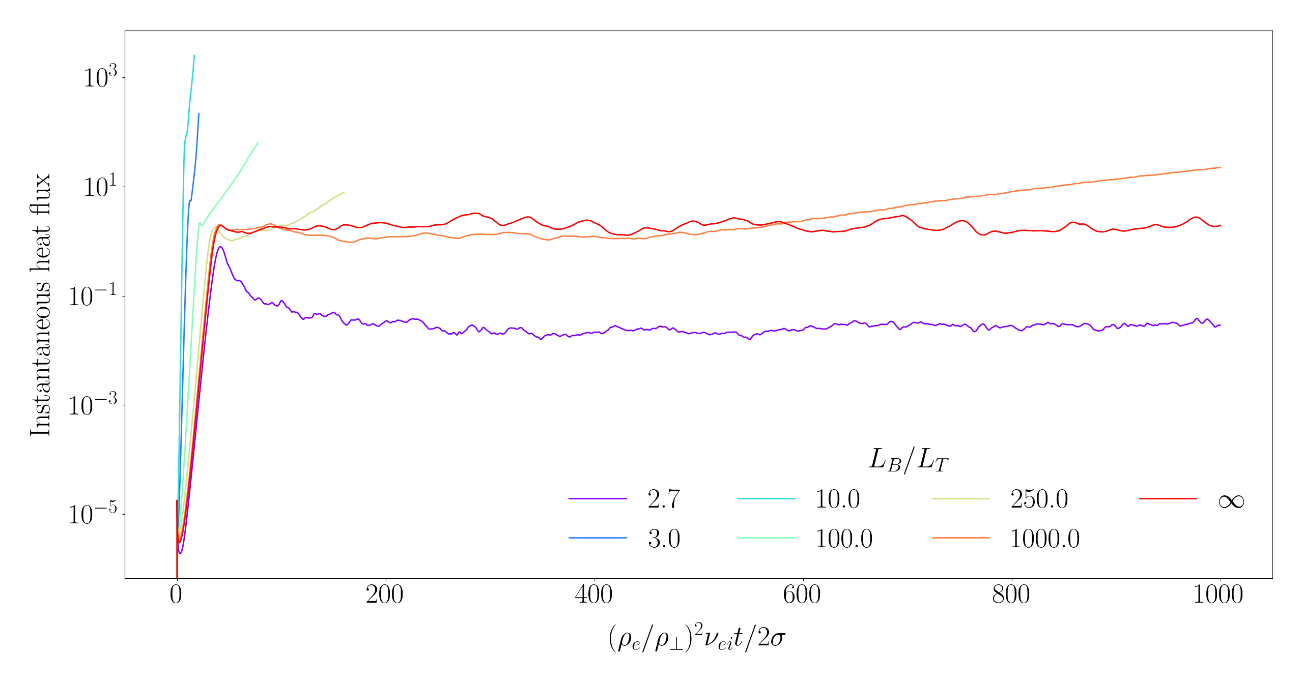
Figure 13: Time traces of the instantaneous heat flux from simulations with finite $L_{B}/L_{T}$, with the limit of $L_{B}/L_{T}\rightarrow\infty$ shown for comparison. All parameters are the same as the baseline simulation (see table 1), and the heat flux is normalised to $(\rho_{\perp}/\rho_{e})Q_{\text{gB}e}$. The heat flux grows without bound in all simulations with (finite) $L_{B}/L_{T}$ above the linear critical gradient eq. 137 ($\approx 2.72$ for $\bar{\tau}=1$), with the rate of divergence decreasing as $L_{B}/L_{T}$ is increased.

As discussed in section 5.5, the adiabatic ion response eq. 14 causes the nonlinearity in the electron-scale continuity equation eq. 15 to vanish identically, a property that is shared by eq. 135, meaning that the system lacks any nonlinearity capable of generating two-dimensional secondary instabilities that are responsible for the generation of zonal flows and destruction of streamer structures (see references in section 5.5). Indeed, the lack of saturation in the case of our ETG simulations appears to be due to the inability of the system to break apart the streamers created by the cETG instability; the existence of such streamers causes the heat flux to diverge as they ‘short circuit’ the heat transport across the radial domain. Even if the simulation initially appears to saturate after the linear phase, it eventually forms these large-scale streamers, which appear to be immune to all types of nonlinear shearing, as seen clearly in the real-space snapshots of cETG turbulence shown in figures 15 and 15.

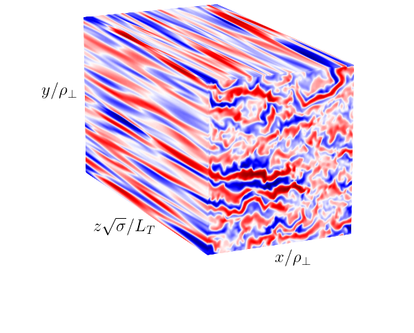
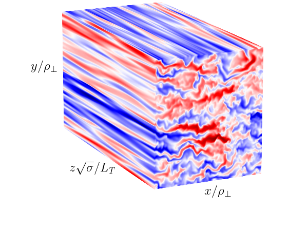
(a) $(L_{T}/\rho_{\perp})\varphi$	(b) $(L_{T}/\rho_{\perp})\delta T_{e}/T_{0e}$

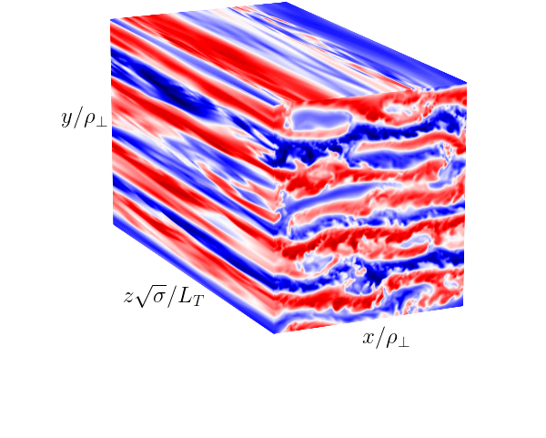
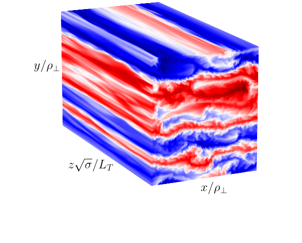
Figure 14: Real-space snapshots of the (a) electrostatic potential and (b) temperature perturbations from the simulation with $L_{B}/L_{T}=1000$ from fig. 13, taken at $(\rho_{e}/\rho_{\perp})^{2}\nu_{ei}t/2\sigma=200$. The coordinate axes are as shown, while the red and blue colours correspond to regions of positive and negative fluctuation amplitude. At these early times, the turbulence appears similar to that of saturated sETG turbulence for $L_{B}/L_{T}\rightarrow\infty$ (cf. fig. 11), despite the eventual lack of saturation (see fig. 15).

(a) $(L_{T}/\rho_{\perp})\varphi$	(b) $(L_{T}/\rho_{\perp})\delta T_{e}/T_{0e}$

Figure 15: The same as fig. 15, except taken at $(\rho_{e}/\rho_{\perp})^{2}\nu_{ei}t/2\sigma=1000$. The unbounded growth of the heat flux is associated with the formation of large-scale, approximately two-dimensional streamer structures that appear to be immune to all types of nonlinear shearing.

This perhaps confirms the view of Hammett et al. (1993) that the adiabatic ion response eq. 14 is insufficient to saturate ETG-scale turbulence in the presence of finite magnetic-field gradients, and one may have to resort to more inclusive closures for the ions. One such closure including scales comparable to the ion-Larmor radius is (see, e.g., Adkins et al., 2022)

$$\frac{\delta n_{e}}{n_{0e}}=-\bar{\tau}^{-1}\varphi+\frac{1}{n_{0i}}\int\mathrm{d}^{3}{\boldsymbol{v}}\>\left<g_{i}\right>_{{\boldsymbol{r}}},$$ (138)

where $\bar{\tau}^{-1}$ is now an operator defined as follows:

$$-\bar{\tau}^{-1}\varphi=-\frac{Z}{\tau}(1-\hat{\Gamma}_{0})\varphi\approx\left\{\begin{array}[]{cc}\displaystyle\frac{Z}{2\tau}\rho_{i}^{2}{\boldsymbol{\nabla}}_{\perp}^{2}\varphi,&\displaystyle k_{\perp}\rho_{i}\ll 1,\\[11.38109pt] \displaystyle-\frac{Z}{\tau}\varphi,&\displaystyle k_{\perp}\rho_{i}\gg 1,\end{array}\right.$$ (141)

and the operator $\hat{\Gamma}_{0}$ can be expressed in Fourier space in terms of the modified Bessel function of the first kind: $\Gamma_{0}=I_{0}(\alpha_{i})e^{-\alpha_{i}}$, where $\alpha_{i}=(k_{\perp}\rho_{i})^{2}/2$. The presence of the non-adiabatic ion distribution function $g_{i}$ in eq. 138, however, means that one would have also to include a self-consistent treatment of ions in order to make use of this closure ($g_{i}=0$ is not a solution to the ion gyrokinetic equation in the presence of finite magnetic drifts). Should this, or other similar closures, allow for saturation, this would imply that one must always appeal to (elements of) ion-scale physics for saturation of electrostatic cETG-driven turbulence. The extent to which such considerations are practically relevant, however, depends on whether or not the system being considered contains any electromagnetic physics, and thus on the value of the (electron) plasma beta $\beta_{e}$. Indeed, for $\beta_{e}\gtrsim m_{e}/m_{i}$, the “flux-freezing scale” $d_{e}=\rho_{e}/\sqrt{\beta_{e}}$ is encountered before (i.e., is smaller than) the ion Larmor radius $\rho_{i}$ when moving towards larger perpendicular scales. Provided that the wavenumber interval between $d_{e}$ and $\rho_{i}$ is sufficiently wide to allow for the presence of electron-scale, electromagnetic instabilities, the mechanisms of saturation in such a system could be vastly different than in the electrostatic regime. This is a subject of ongoing research.

References

- Abel & Cowley (2013) Abel, I. G. & Cowley, S. C. 2013 Multiscale gyrokinetics for rotating tokamak plasmas: II. Reduced models for electron dynamics. New J. Phys. 15, 023041.
- Abel et al. (2013) Abel, I. G., Plunk, G. G., Wang, E., Barnes, M., Cowley, S. C., Dorland, W. & Schekochihin, A. A. 2013 Multiscale gyrokinetics for rotating tokamak plasmas: fluctuations, transport and energy flows. Rep. Prog. Phys. 76, 116201.
- Adkins et al. (2022) Adkins, T., Schekochihin, A. A., Ivanov, P. G. & Roach, C. M. 2022 Electromagnetic instabilities and plasma turbulence driven by electron-temperature gradient. J. Plasma Phys. 88, 905880410.
- Adkins (2023) Adkins, T. G. 2023 Electromagnetic instabilities and plasma turbulence driven by the electron-temperature gradient. PhD thesis, University of Oxford (URL: https://ora.ox.ac.uk/objects/uuid:337d61a1-7997-435c-975e-4928cc3902ea).
- Adkins & Schekochihin (2018) Adkins, T. G. & Schekochihin, A. A. 2018 A solvable model of Vlasov-kinetic plasma turbulence in Fourier-Hermite phase space. J. Plasma Phys. 84, 905840107.
- Barnes et al. (2011) Barnes, M., Parra, F. I. & Schekochihin, A. A. 2011 Critically balanced ion temperature gradient turbulence in fusion plasmas. Phys. Rev. Lett. 107, 115003.
- Beer & Hammett (1996) Beer, M. A. & Hammett, G. W. 1996 Toroidal gyrofluid equations for simulations of tokamak turbulence. Phys. Plasmas 3, 4046.
- Boldyrev (2005) Boldyrev, S. 2005 On the spectrum of magnetohydrodynamic turbulence. Astrophys. J. 626, L37.
- Braginskii (1965) Braginskii, S. I. 1965 Transport processes in a plasma. Rev. Plasma Phys. 1, 205.
- Candy et al. (2007) Candy, J., Waltz, R. E., Fahey, M. R. & Holland, C. 2007 The effect of ion-scale dynamics on electron-temperature-gradient turbulence. Plasma Phys. Control. Fusion 49, 1209.
- Chapman-Oplopoiou et al. (2022) Chapman-Oplopoiou, B., Hatch, D. R., Field, A. R., Frassinetti, L., Hillesheim, J., Horvath, L., Maggi, C. F., Parisi, J., Roach, C. M., Saarelma, S. & Walker, J. 2022 The role of ETG modes in JET–ILW pedestals with varying levels of power and fuelling. Nucl. Fusion 62, 086028.
- Cho & Lazarian (2004) Cho, J. & Lazarian, A. 2004 The anisotropy of electron magnetohydrodynamic turbulence. Astrophys. J. 615, L41.
- Colyer et al. (2017) Colyer, G. J., Schekochihin, A. A., Parra, F. I., Roach, C. M., Barnes, M. A., Ghim, Y.-c. & Dorland, W. 2017 Collisionality scaling of the electron heat flux in ETG turbulence. Plasma Phys. Control. Fusion 59, 055002.
- Connor & Taylor (1977) Connor, J. W. & Taylor, J. B. 1977 Scaling laws for plasma confinement. Nucl. Fusion 17, 1047.
- Cowley et al. (1991) Cowley, S. C., Kulsrud, R. M. & Sudan, R. 1991 Considerations of ion-temperature-gradient-driven turbulence. Phys. Fluids B 3, 2767.
- Diamond et al. (2005) Diamond, P. H., Itoh, S.-I., Itoh, K. & Hahm, T. S. 2005 Zonal flows in plasma—a review. Plasma Phys. Control. Fusion 47, 35.
- Dorland & Hammett (1993) Dorland, W. & Hammett, G. W. 1993 Gyrofluid turbulence models with kinetic effects. Phys. Fluids B 5, 812.
- Dorland et al. (2000) Dorland, W., Jenko, F., Kotschenreuther, M. & Rogers, B. N. 2000 Electron temperature gradient turbulence. Phys. Rev. Lett. 85, 5579.
- Field et al. (2023) Field, A., Chapman-Oplopoiou, B., Connor, J., Frassinetti, L., Hatch, D., Roach, C., Saarelma, S. & JET contributors 2023 Comparing pedestal structure in JET-ILW H-mode plasmas with a model for stiff ETG turbulent heat transport. Philos. Trans. R. Soc. London A 381, 20210228.
- Goldreich & Sridhar (1995) Goldreich, P. & Sridhar, S. 1995 Toward a theory of interstellar turbulence. 2: Strong Alfvénic turbulence. Astrophys. J. 438, 763.
- Guttenfelder et al. (2022) Guttenfelder, W., Battaglia, D. J., Belova, E., Bertelli, N., Boyer, M. D., Chang, C. S. & et al. 2022 NSTX-U theory, modeling and analysis results. Nucl. Fusion 62, 042023.
- Guttenfelder & Candy (2011) Guttenfelder, W. & Candy, J. 2011 Resolving electron scale turbulence in spherical tokamaks with flow shear. Phys. Plasmas 18, 022506.
- Guttenfelder et al. (2021) Guttenfelder, W., Groebner, R. J., Canik, J. M., Grierson, B. A., Belli, E. A. & Candy, J. 2021 Testing predictions of electron scale turbulent pedestal transport in two DIII-D ELMy H-modes. Nucl. Fusion 61, 056005.
- Hammett et al. (1993) Hammett, G. W., Beer, M. A., Dorland, W., Cowley, S. C. & Smith, S. A. 1993 Developments in the gyrofluid approach to tokamak turbulence simulations. Plasma Phys. Control. Fusion 35, 973.
- Hammett et al. (1992) Hammett, G. W., Dorland, W. & Perkins, F. W. 1992 Fluid models of phase mixing, Landau damping, and nonlinear gyrokinetic dynamics. Phys. Fluids B 4, 2052.
- Hammett & Perkins (1990) Hammett, G. W. & Perkins, F. W. 1990 Fluid moment models for Landau damping with application to the ion-temperature-gradient instability. Phys. Rev. Lett. 64, 3019.
- Hardman et al. (2022) Hardman, M. R., Parra, F. I., Chong, C., Adkins, T., Anastopoulos-Tzanis, M. C., Barnes, M., Dickinson, D., Parisi, J. F. & Wilson, H. R. 2022 Extended electron tails in electrostatic microinstabilities and the nonadiabatic response of passing electrons. Plasma Phys. Control. Fusion 64, 055004.
- Hardman et al. (2023) Hardman, M. R., Parra, F. I., Patel, B. S., Roach, C. M., Ruiz Ruiz, J., Barnes, M., Dickinson, D., Dorland, W., Parisi, J. F., St-Onge, D. & Wilson, H. 2023 New stability parameter to describe low- electromagnetic microinstabilities driven by passing electrons in axisymmetric toroidal geometry. Plasma Phys. Control. Fusion 65, 045011.
- Hasegawa & Mima (1978) Hasegawa, A. & Mima, K. 1978 Pseudo-three-dimensional turbulence in magnetized nonuniform plasma. Phys. Fluids 21, 87.
- Hasegawa & Wakatani (1983) Hasegawa, A. & Wakatani, M 1983 Plasma Edge Turbulence. Phys. Rev. Lett. 50, 682.
- Hatch et al. (2019) Hatch, D. R., Kotschenreuther, M., Mahajan, S. M., Merlo, G., Field, A. R., Giroud, C., Hillesheim, J. C., Maggi, C. F., Perez von Thun, C., Roach, C. M., Saarelma, S. & Contributors, JET 2019 Direct gyrokinetic comparison of pedestal transport in JET with carbon and ITER-like walls. Nucl. Fusion 59, 086056.
- Hatch et al. (2022) Hatch, D. R., Michoski, C., Kuang, D., Chapman-Oplopoiou, B., Curie, M., Halfmoon, M., Hassan, E., Kotschenreuther, M., Mahajan, S. M., Merlo, G., Pueschel, M. J., Walker, J. & Stephens, C. D. 2022 Reduced models for ETG transport in the tokamak pedestal. Phys. Plasmas 29, 062501.
- Hatch et al. (2011) Hatch, D. R., Terry, P. W., Jenko, F., Merz, F. & Nevins, W. M. 2011 Saturation of gyrokinetic turbulence through damped eigenmodes. Phys. Rev. Lett. 106, 115003.
- Helander & Sigmar (2005) Helander, P. & Sigmar, D. J. 2005 Collisional Transport in Magnetized Plasmas. Cambridge: Cambridge University Press.
- Horton et al. (1988) Horton, W., Hong, B. G. & Tang, W. M. 1988 Toroidal electron temperature gradient driven drift modes. Phys. Fluids 31, 2971.
- Hosking & Schekochihin (2022) Hosking, D. N. & Schekochihin, A. A. 2022 Emergence of long-range correlations and thermal spectra in forced turbulence. arXiv e-prints 2202.00462.
- Howes et al. (2006) Howes, G. G., Cowley, S. C., Dorland, W., Hammett, G. W., Quataert, E. & Schekochihin, A. A. 2006 Astrophysical gyrokinetics: basic equations and linear theory. Astrophys. J. 651, 590.
- Ivanov et al. (2022) Ivanov, P. G., Schekochihin, A. A. & Dorland, W. 2022 Dimits transition in three-dimensional ion-temperature-gradient turbulence. J. Plasma Phys. 88, 905880506.
- Ivanov et al. (2020) Ivanov, P. G., Schekochihin, A. A., Dorland, W., Field, A. R. & Parra, F. I. 2020 Zonally dominated dynamics and Dimits threshold in curvature-driven ITG turbulence. J. Plasma Phys. 86, 855860502.
- Jenko et al. (2000) Jenko, F., Dorland, W., Kotschenreuther, M. & Rogers, B. N. 2000 Electron temperature gradient driven turbulence. Phys. Plasmas 7, 1904.
- Joiner et al. (2006) Joiner, N., Applegate, D., Cowley, S. C., Dorland, W. & Roach, C. M. 2006 Electron temperature gradient driven transport in a MAST H-mode plasma. Plasma Phys. Control. Fusion 48, 685.
- Kolmogorov (1941) Kolmogorov, A. N. 1941 Local structure of turbulence in incompressible viscous fluid at very large Reynolds numbers. Dokl. Acad. Nauk SSSR 30, 299.
- Kotschenreuther et al. (1995a) Kotschenreuther, M., Dorland, W., Beer, M. A. & Hammett, G. W. 1995a Quantitative predictions of tokamak energy confinement from first-principles simulations with kinetic effects. Phys. Plasmas 2, 2381.
- Kotschenreuther et al. (1995b) Kotschenreuther, M., Rewoldt, G. & Tang, W. M. 1995b Comparison of initial value and eigenvalue codes for kinetic toroidal plasma instabilities. Comp. Phys. Comms. 88, 128.
- Landau (1946) Landau, L. 1946 On the vibrations of the electronic plasma. Zh. Eksp. Teor. Fiz. 16, 574.
- Lee et al. (1987) Lee, Y. C., Dong, J. Q., Guzdar, P. N. & Liu, C. S. 1987 Collisionless electron temperature gradient instability. The Physics of Fluids 30, 1331.
- Liu (1971) Liu, C. S. 1971 Instabilities in a magnetoplasma with skin current. Phys. Rev. Lett. 27, 1637.
- Nazarenko & Schekochihin (2011) Nazarenko, S. V. & Schekochihin, A. A. 2011 Critical balance in magnetohydrodynamic, rotating and stratified turbulence: towards a universal scaling conjecture. J. Fluid Mech. 677, 134.
- Newton et al. (2010) Newton, S. L., Cowley, S. C. & Loureiro, N. F. 2010 Understanding the effect of sheared flow on microinstabilities. Plasma Phys. Control. Fusion 52, 125001.
- Onsager (1931) Onsager, L. 1931 Reciprocal relations in irreversible processes. I. Phys. Rev. 37, 405.
- Orszag (1971) Orszag, SA 1971 On the elimination of aliasing in finite-difference schemes by filtering high-wavenumber components. J. Atmos. Sci. 28, 1074.
- Parisi et al. (2020) Parisi, J. F., Parra, F. I., Roach, C. M., Giroud, C., Dorland, W., Hatch, D. R., Barnes, M., Hillesheim, J. C., Aiba, N., Ball, J., Ivanov, P. G. & contributors, JET 2020 Toroidal and slab ETG instability dominance in the linear spectrum of JET-ILW pedestals. Nucl. Fusion 60, 126045.
- Parisi et al. (2022) Parisi, J. F., Parra, F. I., Roach, C. M., Hardman, M. R., Schekochihin, A. A., Abel, I. G., Aiba, N., Ball, J., Barnes, M., Chapman-Oplopoiou, B., Dickinson, D., Dorland, W., Giroud, C., Hatch, D. R., Hillesheim, J. C., Ruiz Ruiz, J., Saarelma, S., St-Onge, D. & Contributors, JET 2022 Three-dimensional inhomogeneity of electron-temperature-gradient turbulence in the edge of tokamak plasmas. Nucl. Fusion 62, 086045.
- Patel et al. (2021) Patel, B. S., Dickinson, D., Roach, C. M. & Wilson, H. R. 2021 Linear gyrokinetic stability of a high non-inductive spherical tokamak. Nucl. Fusion 62, 016009.
- Ren et al. (2017) Ren, Y., Belova, E., Gorelenkov, N., Guttenfelder, W., Kaye, S. M., Mazzucato, E., Peterson, J. L., Smith, D. R., Stutman, D., Tritz, K., Wang, W. X., Yuh, H., Bell, R. E., Domier, C. W. & LeBlanc, B. P. 2017 Recent progress in understanding electron thermal transport in NSTX. Nucl. Fusion 57, 072002.
- Roach et al. (2009) Roach, C. M., Abel, I. G., Akers, R. J., Arter, W., Barnes, M., Camenen, Y., Casson, F. J., Colyer, G., Connor, J. W., Cowley, S. C., Dickinson, D., Dorland, W., Field, A. R., Guttenfelder, W., Hammett, G. W., Hastie, R. J., Highcock, E., Loureiro, N. F., Peeters, A. G., Reshko, M., Saarelma, S., Schekochihin, A. A., Valovic, M. & Wilson, H. R. 2009 Gyrokinetic simulations of spherical tokamaks. Plasma Phys. Control. Fusion 51, 124020.
- Roberg-Clark et al. (2022) Roberg-Clark, G. T., Plunk, G. G. & Xanthopoulos, P. 2022 Coarse-grained gyrokinetics for the critical ion temperature gradient in stellarators. Phys. Rev. Res. 4, L032028.
- Rogers et al. (2000) Rogers, B. N., Dorland, W. & Kotschenreuther, M. 2000 Generation and stability of zonal flows in ion-temperature-gradient mode turbulence. Phys. Rev. Lett. 85, 5336.
- Schekochihin (2022) Schekochihin, A. A. 2022 MHD turbulence: a biased review. J. Plasma Phys. 88, 155880501.
- Schekochihin et al. (2009) Schekochihin, A. A., Cowley, S. C., Dorland, W., Hammett, G. W., Howes, G. G., Quataert, E. & Tatsuno, T. 2009 Astrophysical gyrokinetics: kinetic and fluid turbulent cascades in magnetized weakly collisional plasmas. Astrophys. J. Suppl. 182, 310.
- Schekochihin et al. (2016) Schekochihin, A. A., Parker, J. T., Highcock, E. G., Dellar, P. J., Dorland, W. & Hammett, G. W. 2016 Phase mixing versus nonlinear advection in drift-kinetic plasma turbulence. J. Plasma Phys. 82, 905820212.
- Shimomura et al. (2001) Shimomura, Y., Murakami, Y., Polevoi, A. R., Barabaschi, P., Mukhovatov, V. & Shimada, M. 2001 ITER: opportunity of burning plasma studies. Plasma Phys. Control. Fusion 43, 385.
- Sips (2005) Sips, A. C. C. 2005 Advanced scenarios for ITER operation. Plasma Phys. Control. Fusion 47, A19.
- Snyder et al. (1997) Snyder, P. B., Hammett, G. W. & Dorland, W. 1997 Landau fluid models of collisionless magnetohydrodynamics. Phys. Plasmas 4, 3974.
- Spitzer & Härm (1953) Spitzer, L. & Härm, R. 1953 Transport phenomena in a completely ionized gas. Phys. Rev. 89, 977.
- Terry & Horton (1983) Terry, P. W. & Horton, W. 1983 Drift wave turbulence in a low-order space. Phys. Fluids 26, 106.
- Tirkas et al. (2023) Tirkas, S., Chen, H. an Merlo, G., Jenko, F. & Parker, P. 2023 Zonal flow excitation in electron-scale tokamak turbulence. Nucl. Fusion 63, 026015.
- Told et al. (2015) Told, D., Jenko, F., TenBarge, J. M., Howes, G. G. & Hammett, G. W. 2015 Multiscale nature of the dissipation range in gyrokinetic simulations of Alfvénic turbulence. Phys. Rev. Lett. 115, 025003.
- Waltz (1988) Waltz, R. E. 1988 Three-dimensional global numerical simulation of ion temperature gradient mode turbulence. Phys. Fluids 31, 1962.
- Zhu et al. (2020) Zhu, H., Zhou, Y. & Dodin, I. Y. 2020 Theory of the tertiary instability and the dimits shift within a scalar model. J. Plasma Phys. 86, 905860405.