Mapping dynamical systems with distributed time delays to sets of ordinary differential equations

Abstract

Real-world dynamical systems with retardation effects are described in general not by a single, precisely defined time delay, but by a range of delay times. An exact mapping onto a set of $N+1$ ordinary differential equations exists when the respective delay distribution is given in terms of a gamma distribution with discrete exponents. The number of auxiliary variables one needs to introduce, $N$, is inversely proportional to the variance of the delay distribution. The case of a single delay is therefore recovered when $N\to\infty$. Using this approach, denoted here the ‘kernel series framework’, we examine systematically how the bifurcation phase diagram of the Mackey-Glass system changes under the influence of distributed delays. We find that local properties, f.i. the locus of a Hopf bifurcation, are robust against the introduction of broadened memory kernels. Period-doubling transitions and the onset of chaos, which involve non-local properties of the flow, are found in contrast to be more sensitive to distributed delays. In general, the observed effects are found to scale as $1/N$. Furthermore, we consider time-delayed systems exhibiting chaotic diffusion, which is present in particular for sinusoidal flows. We find that chaotic diffusion is substantially more pronounced for distributed delays. Our results indicate in consequence that modeling approaches of real-world processes should take the effects of distributed delay times into account.

^∗ Corresponding author.

1 Introduction

On a fundamental level, all known laws of nature are strictly markovian. An example is the Schrödinger equation, $\hbar\dot{\psi}(\mathbf{x},t)=H\psi(\mathbf{x},t)$, which describes a complex-valued dynamical system for which the time evolution is fully determined by the current state of the system, the wavefunction $\psi(\mathbf{x},t)$. There is no memory. In contrast, delayed effects often emerge in the context of macroscopic processes. The study of effective models containing time delays is hence an important subject [1].

The vast majority of studies dedicated to time delayed systems assume that the delay $T$ is accurately defined [2, 3], with $T$ being either constant or functionally dependent on time, e.g. containing a periodic modulation [4]. Strictly speaking, time delays are however never precisely defined. Consider a dynamical variable $x(t)$ whose time evolution is influenced by past states, say by $x(t-T)$. For this to be possible, the past trajectory must be stored, either explicitly or implicitly, via suitable physical, chemical, or biophysical processes. Memory formation takes however time, which implies that only a washed-out version of the past will be available. Mathematically, the system is hence described not by a fixed time delay, but by distributed time delays.

The broadening of the memory kernel may be disregarded when it is small, which is achievable in particular for technical systems [5]. For natural systems [6], distributed time delays are however prominent. This is well known for epidemic spreading, which can be modeled on a realistic level only with distributed delays [7, 8]. The underlying reason is that biological processes, like incubation and recovery times, are intrinsically variable. A corresponding observation holds for the interaction between tumors and the immune systems [9], or for the delayed responses intrinsic to predator-prey models [10].

It is well-known that dynamical systems with distributed time delays can be mapped onto sets of ordinary differential equations (ODEs) using the so-called “linear chain trick” (see, e.g., [11, 12, 13, 14]). The resulting ODE system takes a particular simple form when the distribution of the delays is described by a gamma distribution with integer exponents. This method, which we denote here the “kernel series framework”, allows for the systematic study of delay differential equations (DDEs) with distributed delays and the influence of broadened memory kernels. It is closely related to previous work in the context of integro-differential equations [15], non-reducible distributed delays [16] and threshold delay systems [17].

For the case of a DDE with discrete time delays, the kernel series framework provides an approximation scheme via a set of $N\!+\!1$ ODEs. This approximation is systematic in the sense that the original DDE is recovered in the limit $N\!\to\!\infty$, with the differences scaling as $1/N$. The kernel series framework allows hence to study delay systems with publicly available scientific software libraries, which contain solvers typically only for sets of ordinary differential equations, but not for delay systems.

The method is reviewed in section 2, where we show that a finite order $N$ of the kernel series corresponds to a delay distribution with a relative width $1/\sqrt{N}$. Subsequently, in section 3, we study analytically and numerically first the delay-induced Hopf bifurcation and then the properties of a prototypical delay dynamical system, the Mackey-Glass system. Comparing the original DDE with the corresponding kernel series framework, we find distinct differences between the local and the global regime. For a good description of the Hopf bifurcation, which depends on local properties of the flow, only a modest number of auxiliary variables is needed, which implies that local bifurcations are robust with respect to washed-out memory kernels.

Period-doubling transitions and delay-induced chaos are phenomena that depend on non-local properties of the flow. In this regime, the global regime, in part substantial differences between DDEs with a single time delay and systems with distributed delays are observed. Even for larger $N$, of the order of a few hundred, both the respective bifurcation points and the topology of the resulting attractors may differ noticeably. This result has important consequences for applications. Globally stabilized dynamical states observed for delay systems in the limiting case of precisely defined time delays may not be present in the corresponding real-world systems characterized by distributed time delays.

In section 4, we discuss the extension of the kernel series framework to general time-delay distributions. Afterwards, in section 5, we consider an application to a system exhibiting diffusive chaotic dynamics, finding that chaotic diffusion is substantially enhanced for distributed delays.

2 Kernel series framework

The dynamics of a dynamical system with time delays depends on its history $h(t)$, as defined by

$$\dot{x}(t)=F\left(t,x(t),h(t)\right)\,,$$ (1)

where $x(t)$ is the primary dynamical variable and $F$ a given function. For a DDE with a single time delay $T$ one has $h(t)=x(t-T)$. In general, the memory $h(t)$ is given by a superposition of past states $x(t-\tau)$,

$$h(t)=\int_{0}^{\infty}x(t-\tau)K(\tau)\,\mathrm{d}\tau,\qquad\quad\int_{0}^{\infty}K(\tau)\,\mathrm{d}\tau=1\,,$$ (2)

where $K(\tau)\geq 0$ is the time delay kernel. A single time delay of size $T$ is present for $K(\tau)=\delta(\tau-T)$.

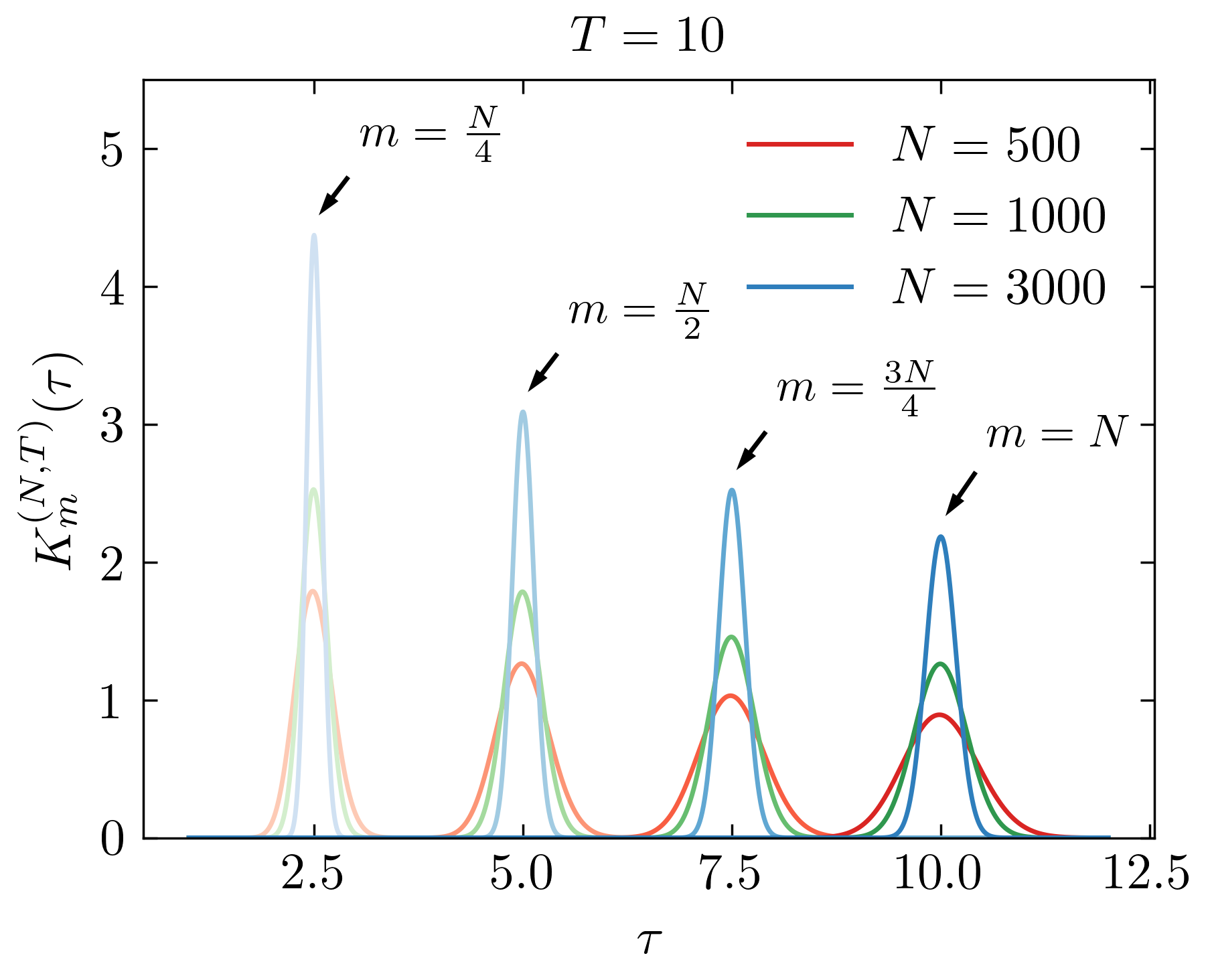
Figure 1: Time delay kernels. The probability densities of $K^{(N,T)}_{m}(\tau)$, as defined by (3), for $T=10$, together with $N=500$ (red lines), $N=1000$ (green lines) and $N=3000$ (blue lines). The four peaks observable for each $N$ correspond respectively to $m/N=1.0,\,0.75,\,0.5,\,0.25$ (progressively shaded lines correspond to distinct $m/N$). The width of the peaks scale as $1/\sqrt{m}$, see (4). The kernels converge to the Dirac delta distributions $\delta(\tau-mT/N)$ in the limit $N\to\infty$.

We concentrate mostly on time delay kernels based on the probability density of the gamma distribution. Later on, in section 4, the general case will be treated. For a given number $N>0$, the order of the framework, we define $N$ kernels

$$K^{(N,T)}_{m}(\tau)=\frac{N^{m}}{(m-1)!\,T^{m}}\,\left[\tau^{m-1}\mathrm{e}^{-N\tau/T}\right],\qquad\quad m=1,\dots,N\,,$$ (3)

which correspond to a set of $N$ normalized gamma distributions. Mean and variance are

$$\mu=\frac{mT}{N},\qquad\quad\sigma^{2}=\frac{mT^{2}}{N^{2}},\qquad\quad\frac{\sigma}{\mu}=\frac{1}{\sqrt{m}}\,,$$ (4)

which implies that

$$\lim_{N\to\infty}K_{N}^{(N,T)}(t)=\delta(t-T)\,.$$ (5)

An illustration of the kernel series is given in figure  1. One observes that the densities converge to a $\delta$-function for $N\to\infty$ when the ratio $m/N$ is kept fixed, in agreement with (4). For a given memory $h(t)$, distributed by a gamma-shaped delay kernel $K(\tau)\propto\tau^{x}\mathrm{e}^{y}$, the corresponding mean time delay $T$ and order $N$ are easily retrieved from the inverse relations

$$T=\frac{x+1}{y},\qquad\quad N=x+1\,.$$

2.1 Equivalence to sets of ordinary differential equations

There are many representations of the Dirac $\delta$-functions commonly used. What makes (3) especially interesting is that the individual kernels can be evaluated by a simple additional ordinary differential equation, which is the essence of the linear chain trick [12, 13, 14, 18]. For this purpose auxiliary variables $x_{m}$ are introduced via

$$x_{m}(t)=\int_{0}^{\infty}x(t-\tau)K_{m}^{(N,T)}(\tau)\,\mathrm{d}\tau,\qquad\quad m=1,\dots,N\,.$$ (6)

At face value, it may seem that one needs to store the full history of $x(t)$ for the evaluation of the convolutions defining the $x_{m}$. This is however not the case. The reason is that the $x_{m}(t)$ form a closed set of recursive differential equations [11, 14, 18],

$$\dot{x}_{m}(t)=\frac{x_{m-1}(t)-x_{m}(t)}{T_{N}},\qquad\quad x_{0}(t)=x(t),\qquad\quad T_{N}=\frac{T}{N}\,,$$ (7)

which holds for $m=1,\,\dots,\,N$. For a derivation one uses

$$\dot{x}_{m}(t) = \int_{0}^{\infty}K_{m}^{(N,T)}(\tau)\frac{\mathrm{d}}{\mathrm{d}t}x_{0}(t-\tau)\,\mathrm{d}\tau$$

$$= -\int_{0}^{\infty}K_{m}^{(N,T)}(\tau)\frac{\mathrm{d}}{\mathrm{d}\tau}x_{0}(t-\tau)\,\mathrm{d}\tau\,$$

with an integration by parts of the last expression leading directly to (7) (see e.g. [14] for a more rigorous proof). Including $x_{0}(t)=x(t)$, one has then a dynamical system defined by $N\!+\!1$ variables $x_{m}(t)$ ($m=0,\dots,N$).

2.2 Kernel series dynamics

The core object of interest is the $(N\!+\!1)$-dimensional dynamical system

$$\cases{\dot{x}_{0}(t)=F\left(t,x_{0}(t),x_{N}(t)\right),\qquad\quad x_{0}(t)=x(t),\\ \dot{x}_{m}(t)=\frac{x_{m-1}(t)-x_{m}(t)}{T_{N}},\qquad\quad m=1,\dots,N\,,}$$ (9)

where $T_{N}=T/N$. It can be viewed from two distinct perspectives. First, that the set of $N\!+\!1$ equations defined by (9) constitutes an exact mapping of a DDE with distributed time delays to a set of ordinary differential equations. This mapping holds when the respective time delay kernel is given by a gamma distribution with an integer exponent. We will show in section 4 that all delay distributions can be mapped to sets of ODEs when the number of auxiliary variables is correspondingly increased. For the most general case, a diverging number of memories $x_{m}(t)$ may however be necessary. Secondly, one can interpret (9) as an approximation,

$$x(t-T)\approx x_{N}(t)\,,$$ (10)

to the delay system defined by (1) when $h(t)=x(t-T)$. In this case the approximation becomes exact in the limit $N\!\to\!\infty$, see (5). For numerical investigations, one can use (9) as a proxy for the original DDE, with the advantage being that standard ODE solvers can be used. In the following we examine in detail what happens when the width of delay distributions is increased or decreased, with distributions of zero width corresponding to the case of a single delay.

2.3 Generalized state history / phase space collapse

The trajectories of a delay system with a single delay $T$ are defined in the space of the state history [19],

$$X(t)=\{x(t^{\prime})\mid t^{\prime}\in[t-T,t)\}\,,$$ (11)

which is formally infinite-dimensional. Consistently, an initial function $\phi\colon[-T,0)\to\mathbb{R}$ is needed for the dynamics defined by (1) when $h(t)=x(t-T)$. Interestingly, one can regard the set of dynamical variables $x_{m}(t)$ defining the kernel series framework, (9), as a generalized state history. The dynamical history is however not sampled at specific points in time, as it would be the case for a discretized version of the standard state history. Instead, suitably weighted superpositions of the past trajectory are taken.

The discretized version of the classical state history (11) can be used to formulate a basic approximation to a DDE in terms of discretized Euler updatings [19]. In contrast to the ODE system (9), Euler updating schemes do however not incorporate a systematic relation to distributed delay times. The result, that the kernel series framework is an exact representation of DDEs with gamma-distributed delay distributions with integer exponents, raises an interesting question. In general, delay systems come with a formally infinite-dimensional state space, which does however collapse, as a corollary of above observation, for specific delay distributions. An interesting point regards the condition for this phase space collapse, namely if it could occur also for other types of delay distributions. We leave these questions for further investigations.

3 Results

We examined extensively the differences showing up between the kernel series framework and the respective original delay equation. We find that lower-order bifurcation transitions agree well already for modest $N$, which is however not the case for chaotic attractors. In particular, we find that chaos tends to disappear when distributions of delays are considered, even when the width of delays is comparatively small.

For the presentation of the results we distinguish between a local and a global regime, noting that the stability of a fixpoint is determined by the local properties of the flow, with the properties of chaotic attractors being determined by non-local, viz global properties of the flow [20]. The same holds for period-doubling transitions.

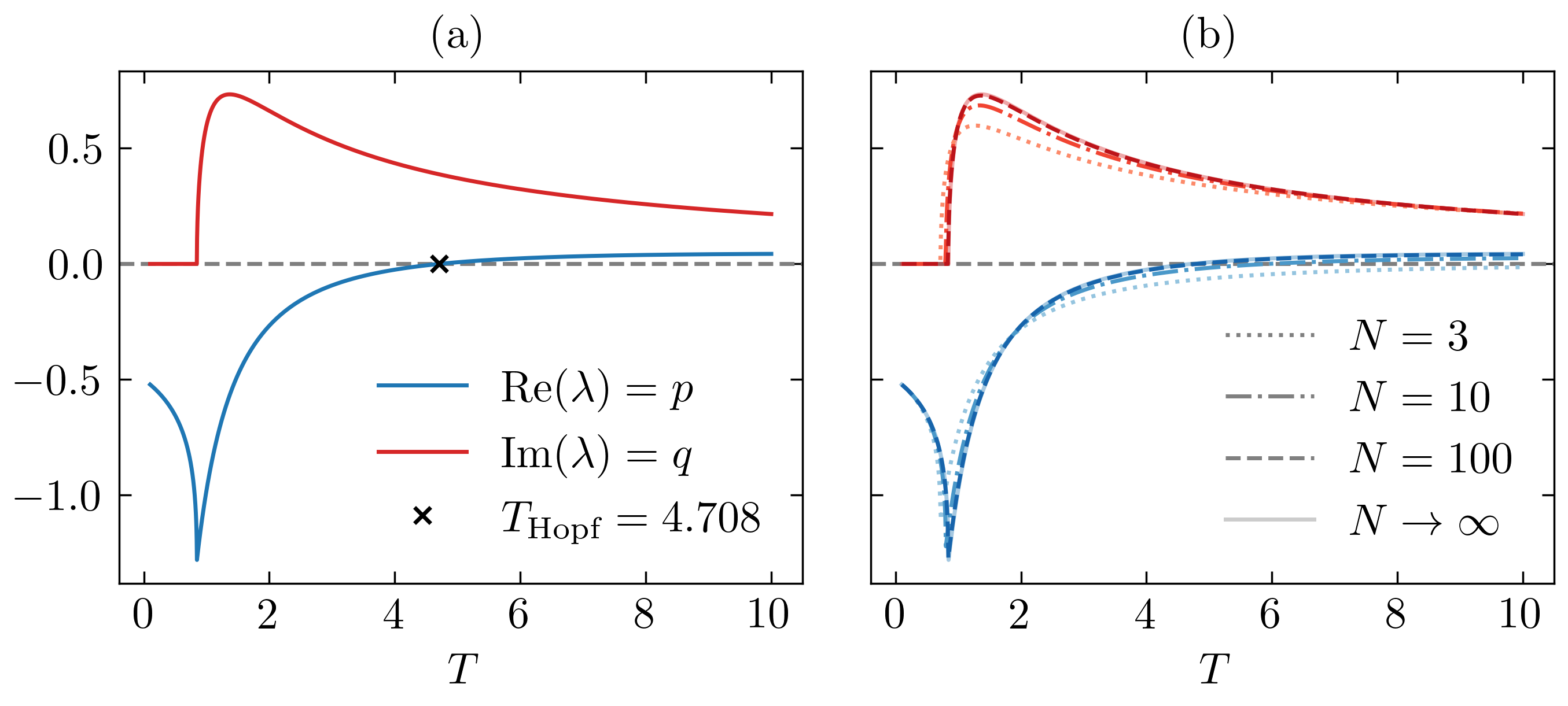
Figure 2: Hopf bifurcation. (a) As a function of the time delay $T$, the real and imaginary part of the numerical solution of (13) for $\lambda=p+\mathrm{i}q$, where the parameters of the linear delay system (12) are $a=0.4$ and $b=0.1$. A Hopf bifurcation occurs at $T_{\mathrm{Hopf}}$ when $\lambda$ crosses the imaginary axis, i.e. when $\mathrm{Re}(\lambda)=p=0$. (b) The exponent $\lambda$ obtained from solving the analytic expression (16) for the kernel series framework compared to the solution shown in (a) obtained for the linear delay system (12) which is found in the kernel series framework by taking the limit $N\to\infty$. Shown are results for $N=3,\,10,\,100$.

3.1 Local regime: Hopf bifurcation

As a first example we study the generic delay system

$$\dot{x}(t)=-c-bx(t)-ax(t-T)\,,$$ (12)

which emerges when expanding (1) with $h(t)=x(t-T)$ around a given fixpoint. It is amenable to an analytic solution [20]. To simplify discussions, we choose $c=0$, which moves the fixpoint of the system to $x^{*}=x(t)=x(t-T)=0$.

The fixpoint $x^{*}$ is stable for $b,\,a>0$ when the time delay $T$ is small. The ansatz $x(t)=C\exp(\lambda t)$ leads to

$$0=\lambda+b+a\mathrm{e}^{-\lambda T}\,.$$ (13)

A Hopf bifurcation occurs at a critical time delay $T_{\mathrm{Hopf}}$ when the real part of $\lambda=p+\mathrm{i}q$ vanishes, viz when $\lambda$ crosses the imaginary axis. One finds

$$b=-a\cos(qT_{\mathrm{Hopf}}),\quad q=a\sin(qT_{\mathrm{Hopf}}),\quad T_{\mathrm{Hopf}}=\frac{\arccos{(-b/a)}}{\sqrt{a^{2}-b^{2}}}.$$ (14)

A numerical solution of (13) is presented in figure 2. We use $a=0.4$ and $b=0.1$, which is consistent with the values of the linearized Mackey-Glass system, as discussed in section 3.2. The Hopf bifurcation point is then $T_{\mathrm{Hopf}}=4.708$.

The kernel series framework (9) for the linear delay system (12) leads to a linear system of $N+1$ coupled ordinary differential equations. The fixpoint, which corresponds to $x_{m}=0$ for $m=0,\dots,N$, has the Jacobian

$$\mathbf{J}=\frac{1}{T_{N}}\left(\matrix{-bT_{N}&&&-aT_{N}\cr 1&-1&&\cr&\ddots&\ddots&\cr&&1&-1}\right)\,,\qquad\quad T_{N}=\frac{T}{N}\,.$$ (15)

The $N+1$ eigenvalues are retrieved from the roots of the characteristic polynomial $P_{N}(\lambda)$, which can be extracted analytically,

$$P_{N}(\lambda)=(b+\lambda)(1+T_{N}\lambda)^{N}+a\,.$$ (16)

As expected, the expression (13) for a single time delay $T$ is recovered in the limit $N\to\infty$ when using $\exp(x)=\lim_{k\to\infty}(1+x/k)^{k}$ together with $T_{N}=T/N$.

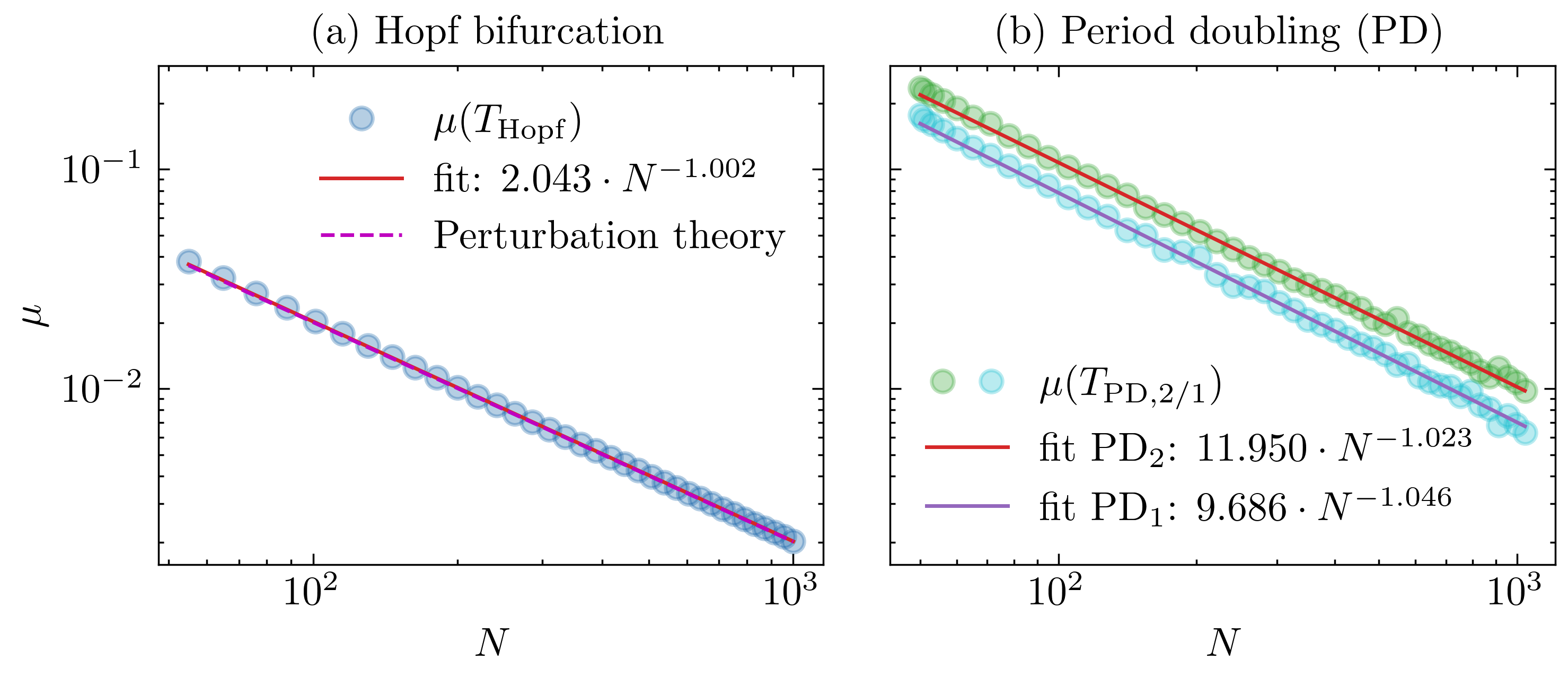
Figure 3: Relative differences. Logarithmic representation of the relative differences between the Hopf bifurcation point and the first and second period doubling bifurcation points obtained within kernel series frameworks of order $N$, (9), and the value found by solving the delay system obtained correspondingly in the limit $N\!\to\!\infty$. (a) For $a=0.4$ and $b=0.1$, the relative deviation $\mu=\mu(T_{\mathrm{Hopf}})$ of the Hopf bifurcation point, as defined by (17). One observes excellent agreement between a linear fit (red line) and the analytic $1/N$ expansion (dashed magenta line), as given by (27), which we derive in the Appendix. (b) The relative deviation $\mu=\mu(T_{\mathrm{PD}})$ of the first (PD₁, blue circles) and second (PD₂, green circles) period doubling transitions, together with linear fits (purple/red lines). For a given order $N$, the relative deviation is generally lowest for the Hopf bifurcation, and lower for the first period doubling than for the second.

The dynamics of the system, and in particular its stability, is dictated by the maximal eigenvalue of the Jacobian $\lambda_{\mathrm{max}}$. In figure 2 we included results for $\lambda_{\mathrm{max}}$ obtained by solving (16) numerically for various orders $N$ of the kernel series framework. The resulting maximal eigenvalues converge quickly towards the ones found for the original system as $N$ increases, as shown in figure 2.

To further quantify the differences between distributed and single time delays we evaluated the relative deviation of the $N$th order result for the Hopf bifurcation point, $T^{(N)}_{\mathrm{Hopf}}$, from the value found for a single time delay (14) using

$$\mu(T_{\mathrm{Hopf}})=\frac{\left|T_{\mathrm{Hopf}}-T^{(N)}_{\mathrm{Hopf}}\right|}{T_{\mathrm{Hopf}}},\qquad\quad T_{\mathrm{Hopf}}=\lim_{N\to\infty}T^{(N)}_{\mathrm{Hopf}}$$ (17)

The numerical results, as well as a power-law fit to the data, are shown in figure 3 (a). We further compare to the analytical prediction attained via perturbation theory, as presented in the Appendix. Asymptotically, the relative deviation $\mu(T_{\mathrm{Hopf}})$ scales as $1/N$, inversely with the order of the kernel series. Quantitatively an agreement of 5% is achieved by $N\approx 39$, and 1% for $N\approx 225$.

Here we also treat the notable case of exponentially distributed delays that emerge for $N=1$. The corresponding characteristic polynomial only has solutions for negative real part of the eigenvalue and thus no Hopf transition is observed. This implies that for all $T$ the dynamics are governed by the stable fixpoint.

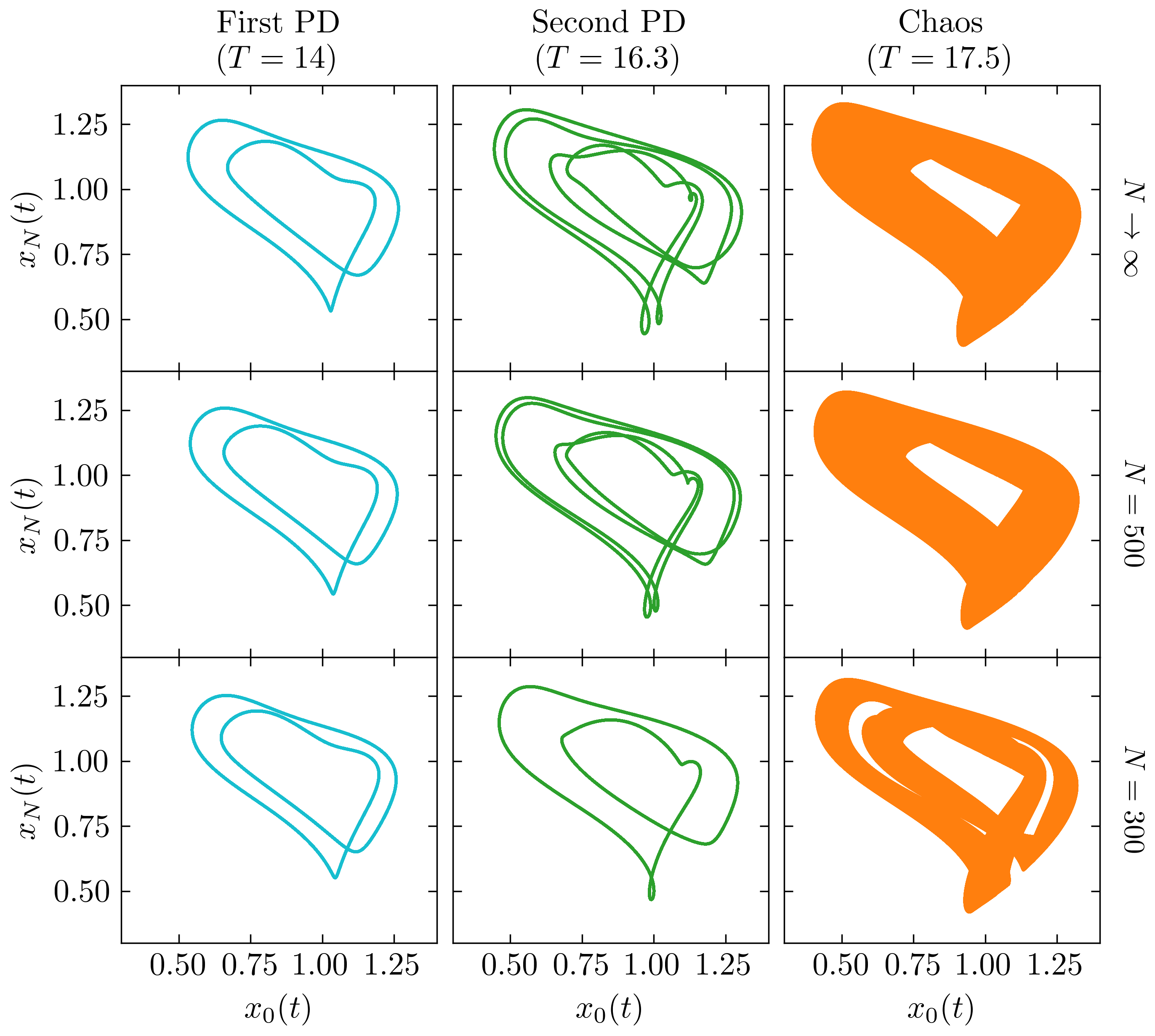
Figure 4: Mackey-Glass system. The stroboscopic projection $(x_{0}(t),x_{N}(t))$ of attractors of the Mackey-Glass system (18), where $x_{0}(t)\to x(t)$ and $x_{N}\to x(t-T)$ for $N\to\infty$. Shown are numerical solutions of the original delay differential equation (top row), and the respective $N$th-order kernel framework, namely for $N=500$ and $N=300$ (middle and bottom row). The average time delay $T$ is chosen such that the original system is beyond the first period doubling (PD, left column), the second PD (middle column), or in the chaotic regime (right column). Substantial differences can be seen between the system with a single time delay (top row) and distributed delays when $N$ is not overly large (bottom row).

3.2 Global regime

For the study of the influence of distributed time delays in the global regime, we consider a prototypical time delay system with chaotic attractors, the Mackey-Glass system,

$$\dot{x}(t)=\frac{\alpha x(t-T)}{1+\left(x(t-T)\right)^{\gamma}}-\beta x(t),\quad\qquad\alpha,\beta,\gamma,T>0\,,$$ (18)

originally introduced to model the production of blood cells [21]. In the following, we set the parameters to the standard values $\alpha=0.2$, $\beta=0.1$, together with $\gamma=10$ [1, 19]. This choice of parameters ensures that the trivial fixpoint $x_{1}^{*}=0$ is unstable for all time delays, while the fixpoint $x_{2}^{*}=(\alpha/\beta-1)^{1/\gamma}=1$ looses stability via a Hopf bifurcation when increasing the delay. In the following we examine to which extent the sequence of bifurcations occurring in (18) changes when the relative width $\sigma/\mu=1/\sqrt{N}$, see (4), of the delay distribution becomes positive. For an overview of state-of-the-art studies of the Mackey-Glass see f.i. [1, 19].

For small time delays, the dynamics are governed by the stable fixpoint $x_{2}^{*}$. Linearizing (18) around $x_{2}^{*}$ and inserting an exponential ansatz yields (13) with $b=0.1$ and $a=0.4$, the parameter values used in section 3.1. A supercritical Hopf bifurcation, destabilizing the fixpoint in favor of a stable limit cycle occurs at $T_{\mathrm{Hopf}}\approx 4.708$, as determined by (14). When further increasing the time delay, the system undergoes a series of period doubling bifurcations (the first two at $T_{\mathrm{PD},1}\approx 13.39$ and $T_{\mathrm{PD},2}\approx 15.95$) and finally, for $T_{\mathrm{Chaos}}\approx 16.5$, a transition to a chaotic regime. We further note that the Mackey-Glass system is strictly dissipative, in the sense that the divergence of the flow is always negative. This holds also for the kernel series framework, viz for distributed time delays, independently of the order $N$.

In figure 4 the stroboscopic projection, plotting $x_{N}(t)\approx x(t-T)$ as a function of $x_{0}(t)=x(t)$, is used to illustrate the topology of the attractors found for three different values of the average time delay, respectively for $T_{\mathrm{PD},1}<T\!=\!14.0<T_{\mathrm{PD},2}$ and $T_{\mathrm{PD},2}<T\!=\!16.3<T_{\mathrm{PD},3}$, as well as for $T=17.5$, which is a bit beyond the onset of chaos. Shown are the attractors obtained by solving (18) directly, denoted as $N\!\to\!\infty$, together with the attractors obtained from the corresponding kernel series framework (9), both for $N=300$ and $500$.

It is clear from figure 4, that the topology of attractors may change once distributions of time delays with positive coefficient of variation are allowed. For example, for $T=16.3$, the resulting limit cycle is doubled only once for $N=300$, but twice for $N=500$ and above. Substantial differences show up in addition for the chaotic attractors stabilizing for $T=17.5$ when the order $N$ is changed. For $N=500$, the stroboscopic projection of the chaotic attractor shown figure 4, seems to be similar, on first sight, to the $N\to\infty$ limit. However, we did not attempt to make a more precise comparison, f.i. in terms of the respective fractal dimensions, which we leave for future studies.

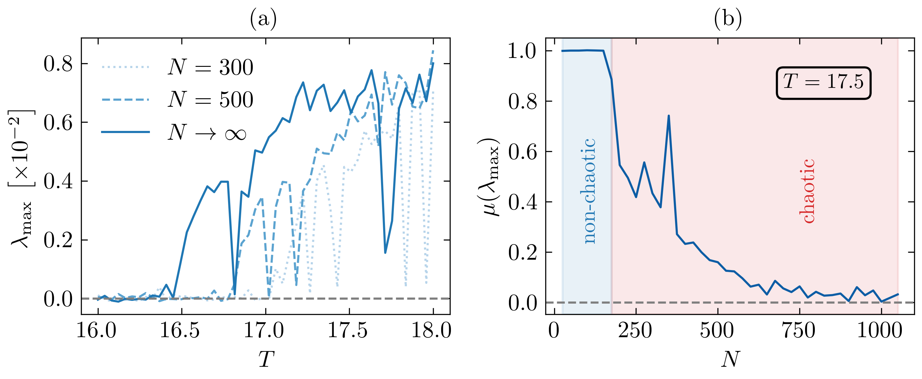
Figure 5: Lyapunov exponents. The maximal Lyapunov exponent $\lambda_{\mathrm{max}}$ of the Mackey-Glass system, see (18). (a) As a function of the average time delay $T$, the Lyapunov exponents obtained from the kernel series framework (9) for different orders, $N=300$ and $N=500$, with $N=\infty$ corresponding to the case of a single delay. (b) For $T=17.5$, the relative deviation of the maximal Lyapunov exponent, obtained respectively for the given $N$ and for $N\to\infty$. For small $N$ (blue shading) the system has not yet entered the chaotic regime (red shading).

In order to quantify the differences between the kernel series framework and the solution of (18), we consider in figure 3 (b) the locus of the bifurcation points of the first and second period doubling, $T_{\mathrm{PD}}$. Shown are the relative differences $\mu$, as defined by (17), between the results obtained numerically for finite $N$ and $N\to\infty$. One finds $1/N$ scaling, in analogy to the behavior observed for the primary Hopf bifurcation, as presented in figure 3 (a). Quantitatively, $\mu=\mu(T_{\mathrm{PD}})$ drops below 5% for the first period doubling when $N>154$, and below 1% for $N>716$ kernels. For larger time delays, larger number of kernels are required – for the second period doubling transition, $\mu$ drops below 5% and 1% respectively for $N>212$ and $N>1020$.

Beyond a cascade of period doubling bifurcations, the Mackey-Glass system enters a chaotic regime. The most common measure for deterministic chaos in dynamical systems is the emergence of one or more positive Lyapunov exponents [20]. The dynamics is dominated by the maximal Lyapunov exponent $\lambda_{\mathrm{max}}$, which quantifies the average spreading of two initially close-by trajectories. Systems with more than one positive Lyapunov exponent are usually called hyperchaotic [24]. In the Mackey-Glass system, we observe a transition to chaos for time delays $T>T_{\mathrm{Chaos}}\approx 16.5$. At this point, the maximal Lyapunov exponent becomes positive, as shown in figure 5 (a). Further on, for $T\gtrsim 27$, the Mackey-Glass system shows hyperchaotic dynamics.

In figure 5 (a) the maximal Lyapunov exponent of the Mackey-Glass system is compared to the maximal Lyapunov exponents of the corresponding kernel series frameworks. The point where the transition to chaos occurs decreases in general with increasing $N$. For $N=500$, we find chaotic behavior for $T\gtrsim 16.8$. In figure 5 (b), the relative deviation of the maximal Lyapunov exponent of the kernel series framework with respect to $N\to\infty$ is plotted over $N$. Systems with $N\lesssim 200$ have not yet transitioned to the chaotic regime at $T=17.5$, which is associated with a kernel width of $\sigma\gtrsim 1.3$. Thus, we note that chaos may break down in the kernel series framework if the kernel width exceeds a threshold value. In this sense, chaos is not robust in the kernel series framework. The peak observed around $N\approx 300$ is caused by a non-chaotic window within the chaotic regime.

3.3 Zero-One test for chaos

The evolution of the cross-correlation of two initially close-by trajectories can be used to classify the long-term dynamical behavior [25]. On defines with $C_{12}(t)$,

$$C_{12}(t)=\frac{\big{\langle}(x_{1}(t)-\bar{x})(x_{2}(t)-\bar{x})\big{\rangle}}{s^{2}}\equiv 1-\frac{D_{12}(t)}{2s^{2}},$$ (19)

the cross-correlation of two trajectories $x_{1}(t)$ and $x_{2}(t)$, where $\bar{x}$ is the center of gravity of the attractor and $s$ the standard deviation. An average $\langle\cdot\rangle$ over initial positions $x_{1}(0)$ and $x_{2}(0)$ is performed, such that the initial distance $\delta=\parallel\!x_{1}(0)-x_{2}(0)\!\parallel$ is kept constant, with $\parallel\!\cdot\!\parallel$ denoting the distance between the respective initial functions. The last term in (19) connects $C_{12}(t)$ with the quadratic distance between the two trajectories, $D_{12}(t)=\langle(x_{1}(t)-x_{2}(t))^{2}\rangle$.

The long-term behavior of chaotic and non-chaotic dynamics differ qualitatively with respect to $C_{12}$ and $D_{12}$, which can be used hence as a One-Zero test for chaos. For the four basic types of attractors one has [25]:

• Fixpoint: A fixpoint attracting both trajectories leads to $D_{12}\to 0$ independently of the initial distance $\delta$.

• Limit Cycle: On average, two trajectories ending up in the same limit cycle have a finite distance that scales with the initial distance. For a limit cycle one has hence $D_{12}\propto\delta$.

• Chaotic Attractor: Independently of the initial distance, trajectories become fully decorrelated on a chaotic attractor. This implies that $D_{12}\propto s^{2}$ for any $\delta>0$.

• Partially Predictable Chaos: In this case the initial exponential divergence is limited by topological constraints, with the final chaotic state being reached only via a subsequent diffusive process, which can be very slow. One has $D_{12}<s^{2}$ for an extended period.

All four states are found in the Mackey-Glass system [25, 19]. In figure 6 the cross-correlation is shown for an average delay $T=17.5$. For large $N$, full decorrelation, viz a decrease of the cross-correlation to essentially zero, occurs within the timescale of the initial exponential decorrelation, which is the hallmark of classical turbulent chaos. Decorrelation is a bit slower for $N=300$, which indicates that the kernel series framework is close to a partially predictable chaotic state in this regime.

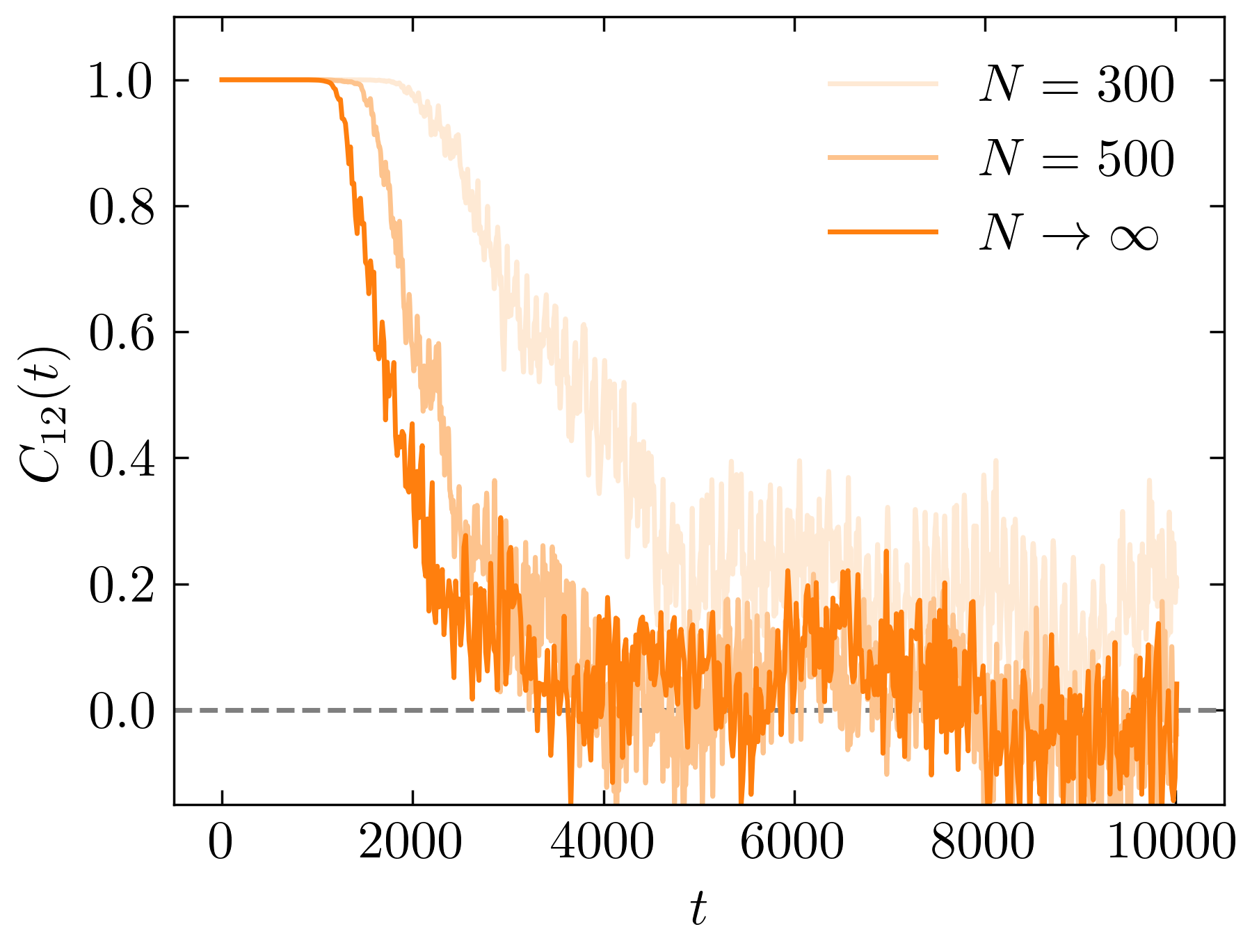
Figure 6: Cross-correlation. As a function of time $t$, the cross-correlation $C_{12}(t)$ of two initially close-by trajectories, as defined by (19). The plots are averages over 100 pairs of initial functions with distances $\delta=10^{-6}$. The average time delay is $T=17.5$, for which the Mackey-Glass system (18) shows normal turbulent chaos. Shown are the results of the kernel series framework (9) for $N=300,500$, together with the cross-correlation of the Mackey-Glass system with a single time delay, denoted by $N\to\infty$.

4 Generic delay distributions

So far we developed the theory for kernel series frameworks that are associated with a delay system containing a single delay $T$. Here we generalized our framework to systems characterized from the start by a pre-determined distribution of time delays.

As a first step we consider systems containing a finite number $M$ of discrete time delays $T_{j}$. Generically, distinct time delays could serve specific functional roles, like in a logistic equation with mixed delays, $\dot{x}(t)=x(t-T_{1})[1-x(t-T_{2})]$. Alternatively, as considered here, the history $h(t)$ entering (1) is assumed to contain $M$ terms with relative weights $\kappa_{j}\geq 0$,

$$h(t)=\sum_{j}\kappa_{j}x(t-T_{j}),\qquad\quad\sum_{j}\kappa_{j}=1\,.$$ (20)

For every time delay $T_{j}$ one constructs a kernel series of length $N_{j}$

$$\left\{K_{i}^{(N_{j},T_{j})}(t)\right\}_{i=1,\dots,N_{j}},\qquad\quad j=1,\dots,M\,,$$ (21)

as defined by (3). In addition, one introduces $\sum_{j}N_{j}$ corresponding auxiliary variables obeying suitably generalized versions of (7).

For a general distribution of time delays, the history is given by

$$h(t)=\int_{0}^{\infty}\kappa(\tau)x(t-\tau)\,\mathrm{d}\tau,\qquad\quad\int_{0}^{\infty}\kappa(\tau)\,\mathrm{d}\tau=1\,,$$ (22)

which generalizes (20). Next one uses the fact that exponential shapelets $\{\psi_{i}(t;\beta)\}_{i\in\mathbb{N}}$ constitute an orthogonal basis on the positive real axis [26]. The delay kernel can hence be expanded in shapelets, as

$$\kappa(t)=\sum_{i}c_{i}\psi_{i}(t;\beta),\qquad\quad c_{i}=\int_{0}^{\infty}\psi_{i}(t;\beta)\kappa(t)\,\mathrm{d}t\,,$$ (23)

where the scale parameter $\beta$ can be used for optimization purposes, e.g. to minimize the number of non-zero expansion coefficients $c_{j}$. Given that exponential shapelets are superpositions of the elementary kernels introduced in (3), one can convert (23) into a kernel series framework, albeit at the cost of a possibly diverging number of auxiliary variables.

5 Chaotic diffusion

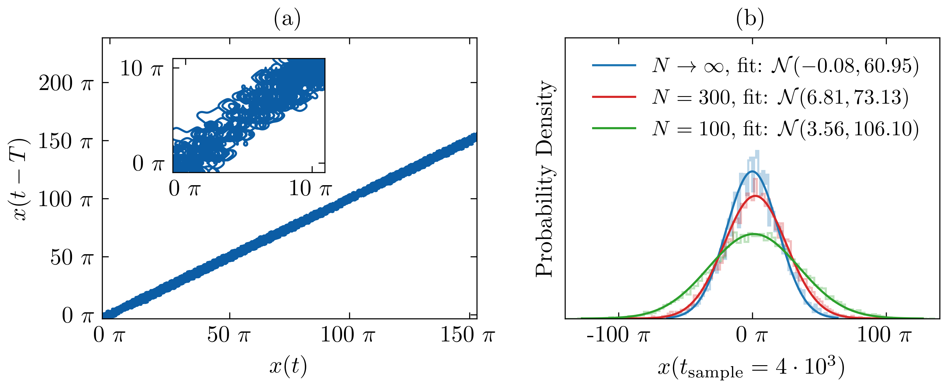
Figure 7: Chaotic diffusion. In (a), for a time delay $T=20$, the stroboscopic projection of the chaotic attractor of (24). The inset shows how the trajectory moves along the band of previously disconnected limit cycles. The trajectory spans the entire real axis, $-\infty<x(t)<\infty$. (b) The probability density for the distance from the origin, also for $T=20$, when sampling at $t_{\mathrm{sample}}=4\cdot 10^{3}$. The three data sets shown correspond to a direct integration of (24) (blue curve) and to the behavior obtained when using the kernel series framework, with orders $N=100,300$ (green and red curve, respectively). A total of $10^{4}$ initial conditions close to the origin have been considered. The data is fitted to a Gaussian $\mathcal{N}(\mu,\sigma)$ with mean $\mu$ and standard deviation $\sigma$, as given in the legend. Chaotic diffusion is more prominent for smaller orders $N$.

So far we investigated the Mackey-Glass system within the kernel series framework. Next we turn towards a time-delayed system exhibiting chaotic diffusion. The flow,

$$\dot{x}(t)=\sin\left(x(t-T)\right)\,,$$ (24)

is given by a time-delayed sinusoidal function. Possible additional parameters, like an overall prefactor, can be eliminated by rescaling $x$ and $t$. The properties of (24) have been studied in detail in [27]. The fixpoints $x^{*}=k\pi$, with $k\in\mathbb{N}$, loose stability in a Hopf bifurcation which gives rise to a stable limit cycle when increasing the time delay $T$. When further increasing the time delay, the period of the limit cycle doubles, with the system transitioning afterwards to a chaotic regime via an attractor-merging crisis. These features are reproduced when using the kernel series framework, with the accuracy increasing as a function of $N$.

Linearizing (24) yields (12) with $a=1$ and $b=c=0$. Therefore, the discussion is qualitatively the same as for the Mackey-Glass system, as given in section 3.1. Again, the relative differences between the loci of the bifurcation points in the time delayed system compared to its representation in the kernel series framework scales as $1/N$, as we did demonstrate previously for the Mackey-Glass system.

In [27] it is noted that (24) shows chaotic diffusion, which implies that the statistics of the trajectory is given in the chaotic regime by 1D Brownian diffusion. This means that the position $x(t_{\mathrm{sample}})$ is normal-distributed when evolving the system up to a sampling time $t_{\mathrm{sample}}\gg 1$ for a number of random initial conditions near the origin. One finds $\mu\to 0$ for the mean [27]. Typical for diffusive behavior is a linearly increasing variance, $\sigma^{2}\sim t_{\mathrm{sample}}$, a behavior that is possible because the chaotic state of (24) forms a band of trajectories from the previously disconnected chain of limit cycles obtained via $2\pi$-shifts [27]. As an illustration, the chaotic attractor of (24) is presented in figure 7 (a) for a time delay of $T=20$. The trajectory spans the entire real axis, $-\infty<x(t)<\infty$ [27].

In figure 7 (b) we numerically evaluate the distribution of $x(t_{\mathrm{sample}})$ for different orders $N=100,300$ of the kernel series framework and compare to the case where (24) is integrated directly ($N\to\infty$), using a sampling time of $t_{\mathrm{sample}}=4\cdot 10^{3}$, $10^{4}$ initial conditions and considering a time delay $T=20$. We find that for different orders $N$ the data is fitted accurately by a Gaussian distribution. The mean remains close to zero for all cases considered. The standard deviation, which is directly related to the diffusion constant, is however strongly dependent on the order $N$, growing in size when lowering $N$. It would be interesting to investigate the scaling of the standard deviation with $1/N$, viz as a function of the variance of the distribution of time delays, which is however computationally demanding. We leave this aspect for future work. In any case our results show that chaotic diffusion is substantially more pronounced when the distribution of time delays has a positive width.

6 Discussion

There are several reasons why distributed time delays are important: Firstly, on a fundamental level, because memory formation takes time, as pointed out in the introduction. Secondly, because natural processes, like the dynamics of blood cells described by the Mackey-Glass system [21], are often intrinsically noisy. For memories of aggregate quantities, like the concentration of cells, biological variability translates into a corresponding distribution function. A similar argument can be made for socio-economic and climate models with delays [28, 29], for which delayed feedback is transmitted in general via a cascade of intermediate processes.

Here we systematically investigated the effects broadened memory kernels have on the dynamics of time delayed systems by replacing discrete delays with distributed delays. It is known (e.g. [14, 18]) that a specific type of delay distributions, gamma distributions with integer exponents, can be mapped exactly onto a set of $N+1$ ordinary differential equations. We here denoted this procedure the ‘kernel series framework’. Gamma distributions take the form of broadened $\delta$-functions, as illustrated in figure 1, which allows to recover the case of a single time delay $T$ as the limiting case $N\to\infty$. The kernel series framework is hence well suited for the systematic study of the influence of distributed time delays on the dynamical phase diagram. Alternatively one may use the kernel series framework as an approximation to a given delay differential equation. From a computational point of view one has to weigh the perks of the kernel series framework against the necessity to solve a much higher dimensional system of differential equations. The complexity of differential equation integration usually scales linearly as $\mathcal{O}(n)$, where $n$ denotes the size of the system [30]. If the required order in the kernel series framework is high, integration may be computationally demanding.

In this paper, we studied numerically the influence of time delay distributions for the Mackey-Glass system as well as a simple time delayed system with sinusoidal nonlinearity. Good agreement is observed in the local regime for the stability of fixed points, for which we prove analytically that corrections scale as $1/N$. We also find that higher-order phenomena, such as period doubling transitions, the occurrence of chaotic dynamics and chaotic diffusion, are substantially more sensitive to the introduction of distributed delays. It may hence be difficult to compare the predictions of dynamical systems with precisely defined time delays with observations, in particular when distributed time delays play an important role in the respective real-world applications.

7 Appendix

7.1 Hopf bifurcation in perturbation theory

An analytical estimate the Hopf bifurcation point occurring within a kernel series framework of order $N$, as defined by (9), may be attained through perturbation theory. In section 3.1 we showed that the characteristic polynomial $P_{N}(\lambda)$ approaches (13) as $(1+x/k)^{k}$ for $k\to\infty$. The relation

$$\left(1+\frac{x}{k}\right)^{k}=\mathrm{e}^{x}\left(1-\frac{x^{2}}{2k}\right)$$ (25)

holds in leading order $1/k$, which is seen by taking the derivative of both sides and comparing in leading order. Inserting (25) into the characteristic polynomial (16), we obtain

$$P_{N}(\lambda)=\lambda+b+a\mathrm{e}^{-\lambda T}-\varepsilon\left[(b+\lambda)\frac{T^{2}\lambda^{2}}{2}\right]=:P_{\infty}(\lambda)+C(\lambda,\varepsilon)=0\,,$$

where $\varepsilon=1/N$ and $C(\lambda,\varepsilon)$ denotes a perturbation of (13), the characteristic equation $P_{\infty}(\lambda)$ of the system containing only a single delay. At the Hopf bifurcation point $T_{\mathrm{Hopf}}$, the real part of $\lambda$ vanishes. Thus, we make the following ansatz at the Hopf bifurcation point for $q:=\mathrm{Im}(\lambda)$ and $T_{\mathrm{Hopf}}$ in terms of $\varepsilon$:

$$q=\sum_{i=0}^{\infty}c_{i}\varepsilon^{i},\qquad T_{\mathrm{Hopf}}=\sum_{i=0}^{\infty}k_{i}\varepsilon^{i}.$$ (26)

In zeroth order the solution (14) found for the DDE is reproduced. In first order we attain

$$k_{1}=\frac{\arccos^{2}(-b/a)\left(b\sqrt{a^{2}-b^{2}}+a^{2}\arccos(-b/a)\right)}{2(a^{2}-b^{2})^{3/2}}\,.$$

For our usual values $a=0.4$ and $b=0.1$ we thus find in first order perturbation theory

$$T_{\mathrm{Hopf}}\simeq 4.708+9.458\cdot\varepsilon,\qquad\quad\varepsilon=\frac{1}{N}\,.$$ (27)

j

Data availability statement

All data that support the findings of this study are included within the article (and any supplementary files).

ORCID ID

C. Gros https://orcid.org/0000-0002-2126-0843
D. H. Nevermann https://orcid.org/0000-0002-4607-5142

References

References

- [1] M Lakshmanan and D V Senthilkumar. Dynamics of nonlinear time-delay systems. Springer Science & Business Media, 2011.
- [2] J Richard. Time-delay systems: an overview of some recent advances and open problems. automatica, 39(10):1667–1694, 2003.
- [3] A Otto, W Just, and G Radons. Nonlinear dynamics of delay systems: an overview. Philosophical Transactions of the Royal Society A, 377(2153):20180389, 2019.
- [4] D Müller, A Otto, and G Radons. Laminar chaos. Physical Review Letters, 120(8):084102, 2018.
- [5] T Erneux, J Javaloyes, M Wolfrum, and S Yanchuk. Introduction to focus issue: Time-delay dynamics, 2017.
- [6] K L Cooke and Z Grossman. Discrete delay, distributed delay and stability switches. Journal of mathematical analysis and applications, 86(2):592–627, 1982.
- [7] E Beretta, T Hara, W Ma, Y Takeuchi, et al. Global asymptotic stability of an sir epidemic model with distributed time delay. Nonlinear analysis, theory, methods & applications, 47(6):4107–4115, 2001.
- [8] C C McCluskey. Complete global stability for an sir epidemic model with delay—distributed or discrete. Nonlinear Analysis: Real World Applications, 11(1):55–59, 2010.
- [9] M Sardar, S Biswas, and S Khajanchi. The impact of distributed time delay in a tumor-immune interaction system. Chaos, Solitons & Fractals, 142:110483, 2021.
- [10] C Xu and Y Shao. Bifurcations in a predator-prey model with discrete and distributed time delay. Nonlinear Dynamics, 67(3):2207–2223, 2012.
- [11] T Gedeon and G Hines. Upper semicontinuity of morse sets of a discretization of a delay-differential equation. Journal of Differential Equations, 151(1):36–78, 1999.
- [12] P Hurtado and C Richards. A procedure for deriving new ode models: Using the generalized linear chain trick to incorporate phase-type distributed delay and dwell time assumptions. Mathematics in Applied Sciences and Engineering, 1(4):412–424, 2020.
- [13] W T Mocek, R Rudnicki, and E O Voit. Approximation of delays in biochemical systems. Mathematical Biosciences, 198(2):190–216, 2005.
- [14] P J Hurtado and A S Kirosingh. Generalizations of the ‘linear chain trick’: incorporating more flexible dwell time distributions into mean field ode models. Journal of mathematical biology, 79(5):1831–1883, 2019.
- [15] R N Valani. Lorenz-like systems emerging from an integro-differential trajectory equation of a one-dimensional wave–particle entity. Chaos: An Interdisciplinary Journal of Nonlinear Science, 32(2):023129, 2022.
- [16] N MacDonald. Stability boundaries for nonreducible distributed delays. Mathematical biosciences, 83(1):49–59, 1987.
- [17] H L Smith. Threshold delay differential equations are equivalent to standard fdes. In International Conference on Differential Equations (Equadiff-91), World Scientific, River Edge, NJ, pages 899–904, 1993.
- [18] T Cassidy. Distributed delay differential equation representations of cyclic differential equations. SIAM Journal on Applied Mathematics, 81(4):1742–1766, 2021.
- [19] H Wernecke, B Sándor, and C Gros. Chaos in time delay systems, an educational review. Physics Reports, 824:1–40, 2019.
- [20] C Gros. Complex and adaptive dynamical systems, a Primer. Springer, 2015.
- [21] M C Mackey and L Glass. Oscillation and chaos in physiological control systems. Science, 197(4300):287–289, 1977.
- [22] Gerrit A. Efficiently and easily integrating differential equations with JiTCODE, JiTCDDE, and JiTCSDE. Chaos, 28(4):043116, 2018.
- [23] L F Shampine, S Thompson, and J Kierzenka. Solving delay differential equations with dde23. URL http://www. runet. edu/~ thompson/webddes/tutorial. pdf, 2000.
- [24] O E Rossler. An equation for hyperchaos. Physics Letters A, 71(2-3):155–157, 1979.
- [25] H Wernecke, B Sándor, and C Gros. How to test for partially predictable chaos. Scientific reports, 7(1):1–12, 2017.
- [26] J Bergé, R Massey, Q Baghi, and P Touboul. Exponential shapelets: basis functions for data analysis of isolated features. Monthly Notices of the Royal Astronomical Society, 486(1):544–559, 2019.
- [27] J C Sprott. A simple chaotic delay differential equation. Physics Letters A, 366(4-5):397–402, 2007.
- [28] A Keane, B Krauskopf, and C M Postlethwaite. Climate models with delay differential equations. Chaos: An Interdisciplinary Journal of Nonlinear Science, 27(11):114309, 2017.
- [29] M Sportelli and L De Cesare. A goodwin type cyclical growth model with two-time delays. Structural Change and Economic Dynamics, 61:95–102, 2022.
- [30] G Ansmann. Efficiently and easily integrating differential equations with jitcode, jitcdde, and jitcsde. Chaos: An interdisciplinary journal of nonlinear science, 28(4):043116, 2018.