$\Delta$-Patching: A Framework for Rapid Adaptation of Pre-trained Convolutional Networks without Base Performance Loss

Abstract

Models pre-trained on large-scale datasets are often fine-tuned to support newer tasks and datasets that arrive over time. This process necessitates storing copies of the model over time for each task that the pre-trained model is fine-tuned to. Building on top of recent model patching work, we propose $\Delta$-Patching for fine-tuning neural network models in an efficient manner, without the need to store model copies. We propose a simple and lightweight method called $\Delta$-Networks to achieve this objective. Our comprehensive experiments across setting and architecture variants show that $\Delta$-Networks outperform earlier model patching work while only requiring a fraction of parameters to be trained. We also show that this approach can be used for other problem settings such as transfer learning and zero-shot domain adaptation, as well as other tasks such as detection and segmentation.

1 Introduction

The proliferation of pre-trained models, especially in the domain of vision tasks, has been remarkable [1]. These models, trained on extensive datasets, possess features that are universally beneficial across a wide array of tasks. Over the years, a significant use of such pre-trained models has been in a fine-tuning or transfer learning context, where the model weights are partially or fully modified while maximizing performance on a target task. While effective, this strategy tends to specialize the model’s features, often at the expense of its original capabilities, causing a decline in performance on the original task for which the model was initially trained. Recently, there have been efforts to “patch” pre-trained models towards improved performance on different target tasks with minimal loss of performance on the original task [19]. Model patching [19] draws parallels with software patching in software engineering and aligns with the growing trend of treating machine learning models as open-source software [34, 19].

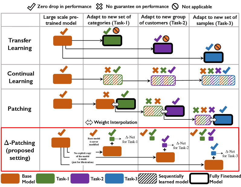
Figure 1: Comparison of $\Delta$-Patching with relevant learning with limited data paradigms. $\Delta$-Patching ensures there is zero-drop in performance on the base task and $\Delta$-Networks (proposed approach to perform $\Delta$-Patching) use significantly less trainable parameters as compared to existing approaches

In this work, we propose $\Delta$-Patching a novel framework engineered for the swift adaptation of large-scale pre-trained models to new tasks without degrading accuracy on existing tasks. The impetus for $\Delta$-Patching arises from practical needs observed in various industries. Consider, for example, an e-commerce platform equipped with a large-scale apparel classification model. As fashion trends evolve or seasons change, the model pre-trained on a comprehensive dataset encompassing a multitude of apparel categories, must adapt to evolving fashion trends and seasonal variations without losing its proficiency in recognizing existing categories. In the medical realm, a healthcare system employing a pre-trained model for medical image diagnosis might need to detect a newly identified condition from MRI scans, without diminishing its diagnostic accuracy for established conditions like tumors. Contrasting with traditional Incremental/Continual Learning (IL) methods, which risk ”catastrophic forgetting” due to continual modification of the base model, $\Delta$-Patching adopts a different philosophy. It capitalizes on the same large-scale pre-trained model for all tasks, ensuring the preservation of its intrinsic knowledge. While IL methods grapple with balancing new task adaptation and old task performance retention, $\Delta$-Patching bypasses this dilemma. It promises rapid and adaptable integration of new tasks while safeguarding the original capabilities of the pre-trained model. This positions $\Delta$-Patching as a compelling strategy, especially when rapid, flexible adaptation to new tasks, without compromising existing capabilities, is paramount.

As an embodiment to achieve $\Delta$-Patching, we introduce $\Delta$-Networks. While not entirely novel, $\Delta$-Networks excel in terms of efficiency and ease of adaptability, making it a highly effective solution for $\Delta$-Patching. $\Delta$-Networks is a hypernetwork [13] with a twist: it incorporates input-conditioned skip connections for adaptive and efficient patching, all while not modifying a single weight of the original model. While sharing the overarching goal of model adaptability with existing work [19], our approach distinguishes itself in several key aspects. First, while [19] focuses on patching open-vocabulary models like CLIP [33], we focus on general-purpose CNNs, which are ubiquitously used and fine-tuned across various domains. Unlike PAINT [19] that necessitate dual model copies for interpolation [19], $\Delta$-Networks introduces input-conditioned skip connections for patching, leaving the original model weights untouched. The essence of our approach, symbolized by the $\Delta$ in $\Delta$-patching and $\Delta$-networks, lies in the minimal input-conditioned skip connections added. This design facilitates memory-efficient model patching, adaptable to varying memory and computational constraints. Crucially, $\Delta$-Networks is fully differentiable, eliminating the need for model interpolations or empirically determined weight coefficients. Figure 1 illustrates the proposed setting and its difference from earlier work. Table 9 presents a feature-wise comparison of the setting when compared to similar settings in related work. While $\Delta$-Networks are primarily engineered for $\Delta$-Patching, they support a wide range of tasks, like object detection, segmentation and can also be used to improve zero-shot domain adaption, transfer learning. The simplicity of our method is its strength. In fact, $\Delta$-Networks achieve new state-of-the-art for transfer learning by improving the performance of an existing transfer learning method. Our key contributions can be summarized as follows:

• Introduction of $\Delta$-Patching, a new model patching strategy that enables rapid adaptation of pre-trained models to new tasks without sacrificing original performance, implemented through $\Delta$-Networks.

• Development of an end-to-end differentiable method that allows patching at varying levels based on computational constraints.

• Extensive evaluation of our methodology across multiple datasets and tasks, demonstrating superior performance with fewer trainable parameters, and setting a new state-of-the-art in transfer learning.

2 $\Delta$-Networks for Efficient Model Patching

Consider a model $\mathcal{M_{S}}$ trained for a base task $\mathcal{T_{S}}$ using samples from a dataset $\mathcal{D_{S}}$. Our primary goal is to patch $\mathcal{M_{S}}$ for performing well on a new task $\mathcal{T_{P}}$ with samples from $\mathcal{D_{P}}$ without any performance degradation on $\mathcal{T_{S}}$. Importantly, we operate under the practical constraints that neither the samples $\mathcal{D_{S}}$ nor any samples generated using $\mathcal{M_{S}}$ are accessible during this process. Let the features learned using $\mathcal{D_{S}}$ for the base/supporting task $\mathcal{T_{S}}$ be denoted as $\mathcal{F_{S}}$. $\mathcal{F_{S}}^{k}$ then denotes a layer (or a block of layers) (for e.g. with convolutional, max-pooling operations and activation functions in a traditional CNN). $\mathcal{F_{S}}$, the final representation learned with samples from $\mathcal{D_{S}}$ can be viewed as a composition of features learned at each layer, and can be written as below for a given input sample $\mathbf{x}_{s}$ from the dataset $\mathcal{D_{S}}$.

$$\mathcal{F_{S}}=\mathcal{F_{S}}^{k}(\mathcal{F_{S}}^{k-1}(\dots(\mathcal{F_{S}}^{1}(\mathbf{x_{s}}))))\vspace{-2pt}$$ (1)

The final model $\mathcal{M_{S}}$ is formed by passing the features $\mathcal{F_{S}}$ into a classification layer/network, denoted using $\phi_{S}$ which typically is a fully-connected layer with neurons equal to the number of classes in $\mathcal{D_{S}}$:

$$\mathcal{M_{S}}=\mathcal{F_{S}}\circ\phi_{S}\vspace{-4pt}$$ (2)

When a new patching task $\mathcal{T_{P}}$ arrives with a corresponding dataset $\mathcal{D_{P}}$, the number of classes in the patching task is generally different from that of the original task. So, adding a new classification layer, $\phi_{P}$ is most often inevitable. Directly modifying $\mathcal{F_{S}}$ to perform better on $\mathcal{T_{P}}$ affects the performance on $\mathcal{T_{S}}$, which defeats our primary goal. We hence introduce an architectural modification to $\mathcal{M_{S}}$ in such a way that it helps address the new task while not affecting the performance on the original task.

As mentioned previously, $\mathcal{F}^{k}$ denotes a sub-block of layers inside $\mathcal{M_{S}}$. Most modern-day architectures stack sub-blocks to build blocks which are again stacked together to build larger architectures. In a general-purpose CNN architecture such as ResNet [15], $\mathcal{F}^{k}$ is a residual block with one skip connection (we refer to this as a sub-block). The output representation for any $\mathcal{F}^{j}$ which represents a sub-block of layers with one skip connection can be denoted as follows:

$$\mathcal{F}^{j}=\mathcal{F}^{j}(\mathcal{F}^{j-1}(\dots(\mathcal{F}^{1}(\mathbf{x})));\mathbf{W}_{j})+\underbrace{{{\color[rgb]{1,0,0}\mathcal{F}^{j-1}(\mathbf{x};{S_{w}})}}}_{\text{Skip connection}}\vspace{-4pt}$$ (3)

where $\mathbf{W_{j}}$ denotes the weights corresponding to the $j^{\text{th}}$ sub-block and the highlighted term in Eqn 3 refers to the representation learned by the previous sub-block, mapped using a weight matrix ${S_{w}}$. In a standard residual network, this highlighted component is obtained by setting ${S_{w}}=I$, where $I$ is the identity matrix. Generalizing the notion of skip connections using ${S_{w}}$ is a key component of the proposed $\Delta$-Networks methodology.

While most architectures as well as earlier transfer learning/patching literature focus on updating $\mathbf{W}_{j}$, we instead turn our focus to the above generalization of skip connections to leverage the features learned on the base/original task. Firstly, we consider all possible skip connections between each sub-block in a block as possible routes for a given input. (Note that we do not introduce skip connections inside layers of a sub-block to keep the overhead minimal.) Figure 2 shows an illustration.

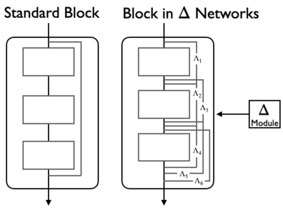
Figure 2: Illustration of a block in $\Delta$-Networks

One could view this as similar to a sparse variant of DenseNets, however with a difference – each connection has a learnable weight matrix ${S_{w}}$ in our case, as described later in this section. The output of a block in Eqn 3 can hence be written as:

$$\mathcal{F}^{j}=\mathcal{F}^{j}(\mathcal{F}^{j-1}(\dots(\mathcal{F}^{1}(\mathbf{x})));\mathbf{W}_{j})+{{\color[rgb]{1,0,0}\sum_{i=1}^{j-1}\mathcal{F}^{i}(\mathbf{x};{S_{w}})}}\vspace{-4pt}$$ (4)

where ${S_{w}}$ is learnable and specifies how two sub-blocks interact. Since this modification does not involve any changes to existing model weights, off-the-shelf pre-trained models can be easily leveraged. Besides, not making any changes to the base model ensures that the performance on the base task is retained without any drop (by simply dropping the added skip connections). Through this generalization, our objective can be viewed as developing a mechanism that allows us to control interactions among pre-trained features at various granularities (for e.g, early vs late layers) so that it enables effective patching for new tasks.

The $\Delta$-module. When learning ${S_{w}}$s for skip connections on top of a pre-trained model for a target task, the same weights that are optimal for one input might be sub-optimal for another input, even from the same dataset or class label. Keeping this in mind, we propose the use of a $\Delta$-module which is a separate, small and lightweight network parameterized by weights $\theta$ that learns the weights of the additional skip connections independent of the base model. Thus, for a given input $\mathbf{x}$, the added skip connections are weighted in an input-conditioned manner using a $\Delta$-module. Following Eqn 4, the output of a sub-block $\mathcal{F}_{j}$ is now changed as follows when a $\Delta$-module (denoted using $\Delta$ below) is introduced:

$${\color[rgb]{1,0,0}\Lambda_{i}=\Delta(\mathbf{x};\theta)}\vspace{-9pt}$$

$$\mathcal{F}^{j}(\textbf{x})=\mathcal{F}^{j}(\mathcal{F}^{j-1}(\dots(\mathcal{F}^{1}(\mathbf{x})));\mathbf{W}_{j})+{\sum_{i=1}^{j-1}\mathcal{F}^{i}(\mathbf{x};{\color[rgb]{1,0,0}\Lambda_{i}})}\vspace{-3pt}$$

Intuitively, we first pass the input to the $\Delta$-module to obtain weighting coefficients $\Lambda_{\{1,\dots(j-1)\}}$ for each of the new skip connections in our $\Delta$-network. Since the $\Delta$-module is a parametrized neural network and therefore fully differentiable, it can be trained directly on the new task loss via gradient descent. Unlike standard skip connections with $\Lambda_{i}=I$, adaptive skip connections have input-conditioned weights on them instead. Since the skip connections are introduced after training, our model can be directly used with existing models that are pre-trained for a different task. (For models that already have skip connections – for example, DenseNets, the $\Lambda_{i}$s for those pre-existing skip connections are defaulted to the identity matrix when addressing the base task.) An end-to-end summary of our approach is provided in Algorithm 1.

Inputs and Initialization:

• Model trained on supporting task $\mathcal{M_{S}}=\mathcal{F_{S}}\circ\phi_{S}$, $\mathcal{F_{S}}\rightarrow\mathcal{F_{S}}^{1\dots k}$ with $k$ blocks;

• Randomly initialized classification head $\phi_{P}$, and $\Delta$-Networks, $\Delta^{1\dots k}$

• Samples from patching task $\mathbf{x_{d}}^{m=1\dots n}\in\mathcal{D_{P}}$ in $n$ batches, Loss function used for the task $\mathcal{L}$

• Add $\phi_{T}$ to $\mathcal{F_{S}}$; Introduce all possible skip connections ($p$) in each sub-block of $\mathcal{F_{S}}^{1\dots k}$

Training:

for num_epochs do

       for $\mathbf{x_{d}}^{m=1\dots n}$ do

             for $j=1\dots k$ do

                   $\Lambda_{1\dots p}=\Delta^{j}(\mathbf{x_{d}^{m}};\theta_{j})$

                   ${\displaystyle\mathcal{F_{S}}^{j}=\mathcal{F_{S}}^{j}(\mathbf{x_{d}^{m}};\mathbf{W_{j}})+\sum_{i=1}^{j-1}\mathcal{F_{S}}^{i}(\mathbf{x_{d}^{m}};\Lambda_{i})}$

                  

             end for

            $\mathcal{M_{P}}=(\mathcal{F_{S}},\Delta^{1\dots k})\circ\phi_{T}$

             Calculate $\mathcal{L}$

             Update $\Delta^{k}$, $\phi_{T}$

            

       end for

      

end for

Output: $\mathcal{F_{S}}\circ\phi_{T}\rightarrow$ model patched for task $\mathcal{T_{P}}$

Algorithm 1 $\Delta$-Networks for Model Patching

Conditioning skip connections using an external fully-differentiable network helps finetune the model easily on a new patching task. When new tasks arrive in a sequence, we introduce a new $\Delta$-module and a classification layer for each task. These $\Delta$-modules are intended to be lightweight (2-layer feedforward networks in our implementation), and hence can be stored easily for each task arriving over time. As each task has its own classifier and $\Delta$-Networks, there is no loss of performance on any of the preceding tasks and the model can support as many tasks as required.

Adapting to Memory/Compute Requirements. When using Algorithm 1, the memory and compute requirements can be controlled using the number of $\Delta$-modules used for a task under consideration. When there are memory/compute constraints, one can choose to use a small $\Delta$-module for learning the weights of skip connections of a few blocks alone. $\Delta$ hence becomes a unit quantum of additional overhead, lending the name $\Delta$-Networks to this approach. With more memory, a set of $\Delta$-modules can be used to learn different skip connections on the base model. The proposed algorithm thus allows customizing $\Delta$-Patching in a memory-sensitive manner. Increasing the number of $\Delta$-modules increases the number of trainable parameters, and hence results in performance gain in general. We provide some design choices and thumb rules of connecting $\Delta$-module to subsets of skip connections in the following section

Implementation and Design Details. Any neural network model developed by stacking sub-blocks of layers can be segregated into a set of blocks, denoted as $\mathcal{F}^{j}$ earlier in this section, with each block containing varying number of sub-blocks. For example, ResNet architectures are often divided into four blocks. If a block contains $k$ sub-blocks, we introduce a total $k(k+1)/2$ skip connections in the block, which is controlled by one $\Delta$-module. One can use additional $\Delta$-modules to weight skip connections in other blocks. We denote $\Delta$-Networks $(n)$ to denote a $\Delta$-network with $n$ $\Delta$-modules. Considering that we only need to learn the weights of the skip connections (and not all parameters of the network), each of our $\Delta$-module consists of a simple two-layer CNN with ReLU activations, normalization layers, and a fully-connected layer to determine the weights for skip connections. The output of a $\Delta$-module is constrained between $[0,1]$ using a sigmoid activation. Whenever skip connections are present in the architecture, there is a problem of increase in variance [52] (we formally show this in the Appendix). With $\Delta$-Networks, when all possible skip connections are introduced, the variance increases rapidly since we add features from all preceding blocks. We address this issue using one BN layer in each $\Delta$-module in our implementation.

3 Experiments and Results

In this section, we aim to provide a holistic evaluation of $\Delta$-Networks, contextualizing its performance against both established and alternative baselines. We first compare $\Delta$-Networks with other relevant methods adapted for the patching setting, and then proceed to a detailed empirical analysis against PAINT[19], the established baseline for model patching.

Beyond patching, we also explore the applicability of $\Delta$-Networks to a range of other tasks, such as object detection and segmentation. Additionally, we examine its performance in specialized settings like zero-shot domain adaptation and transfer learning. To delve deeper into the underlying factors contributing to the success of $\Delta$-Networks, we conclude this section with an ablation analysis.

Experimental Setup: For all the experiments, we leverage CNN models pre-trained on ImageNet, sourced from the official PyTorch [30] and PyTorch Image Models [49] libraries. To ensure a fair comparison, we employ the official code repository of PAINT[19] and apply their method to all models under consideration in our study. In all experiments, both for $\Delta$-Networks and PAINT, we append a fully connected (FC) layer to the model architecture for the new task, consistent with the approach in PAINT. Since PAINT mandates fine-tuning of the entire set of pre-trained weights, we adhere to a 50-epoch fine-tuning regimen for all comparative experiments, utilizing the same data splits and procedures as described in PAINT, to maintain fairness in evaluation. For the experiments where we compare with adapted baselines, we follow the data splits and use the code provided in their official code repositories[35, 36, 27]. Our primary performance metric is the harmonic mean of top-1 accuracies for both pre-trained and fine-tuned tasks, except in the case of sequential patching where we use the mean. Detailed top-1 accuracy scores for individual tasks are available in the appendix for a comprehensive understanding. When deploying $\Delta$-Networks, we introduce one, two, or four $\Delta$-modules. A single $\Delta$-module is added to the last block of the base architecture, complete with corresponding skip connections. For configurations with two or four $\Delta$-modules, they are distributed across the last two or all four blocks of the network, respectively. Each $\Delta$-module incrementally increases the number of trainable parameters, offering a lens through which to study the scalability of $\Delta$-Networks with respect to parameter size and hardware constraints.

3.1 Evaluation of $\Delta$-Networks for Patching

	Flowers	Aircraft	UCF101	GTSRB	DTD	SVHN	CIFAR-100	OmniGlot	Daimler Ped
PAINT	12.73	4.94	21.33	21.36	8.54	62.49	9.27	9.22	18.58
Parallel Adapters [35]	71.46	52.01	73.21	83.20	55.68	81.30	75.52	77.59	83.15
Series Adapters [36]	59.10	46.65	70.67	83.20	39.97	81.34	70.40	77.94	83.11
BatchNormAdapt [27]	71.52	52.52	73.23	83.00	53.20	81.28	75.70	78.07	83.07
$\Delta$-Networks (4)	75.16	58.44	75.52	83.21	56.06	81.52	75.12	78.40	83.16

Table 1: $\Delta$-Networks excels in 8/9 datasets. Comparative Analysis vs. Adapted Methods in $\Delta$-Patching context. Harmonic Mean of Top-1 Accuracies reported.

Architecture	Method	# Parameters	STL10	RESISC45	GTSRB	Flowers	Cars	Aircraft
ResNet-18	PAINT	11.2M	55.41	24.38	18.39	12.70	2.01	3.51
	$\Delta$-Networks (1)	0.4M	79.55	74.48	70.22	75.65	46.78	46.56
	$\Delta$-Networks (2)	0.6M	79.66	76.08	76.20	75.91	51.29	50.48
	$\Delta$-Networks (4)	0.6M	79.57	76.42	78.94	75.65	76.23	52.67
ResNet-34	PAINT	21.8M	62.64	21.91	19.87	16.16	4.39	2.94
	$\Delta$-Networks (1)	0.4M	83.41	78.02	70.83	78.31	47.31	45.74
	$\Delta$-Networks (2)	0.6M	83.59	80.18	78.11	79.04	55.24	51.39
	$\Delta$-Networks (4)	0.6M	83.60	80.70	82.36	78.82	57.33	54.82
ResNet-50	PAINT	23.5M	86.30	48.04	28.11	56.97	12.54	7.33
	$\Delta$-Networks (1)	7.1M	87.53	84.02	77.79	82.64	59.31	55.81
	$\Delta$-Networks (2)	8.9M	87.41	84.93	84.09	82.74	65.96	62.14
	$\Delta$-Networks (4)	9.3M	87.40	85.03	85.67	80.34	67.11	61.48
ConvNeXT-Tiny	PAINT	27.8M	84.57	34.81	12.36	69.06	6.87	6.18
	$\Delta$-Networks (1)	4.0M	89.69	86.54	82.47	87.49	73.00	69.59
	$\Delta$-Networks (2)	5.0M	89.32	86.97	88.01	84.89	75.44	71.74
	$\Delta$-Networks (4)	5.3M	89.35	87.24	88.96	82.35	76.23	70.81

Table 2: $\Delta$-Networks outperforms PAINT with fewer parameters. Comparison in Single-Task Patching across architectures. Harmonic Mean of Top-1 accuracies reported.

Comparison with Adapted Baselines: To situate $\Delta$-Networks within the broader landscape of model patching, we adapt existing methods such as Parallel and Series Adaptors[35, 36], as well as a recent normalization-based approach[27], to the patching setting. The harmonic mean of Top-1 accuracies serves as our performance metric, as mentioned earlier. As shown in Table 1, $\Delta$-Networks outperforms these adapted methods on 8 out of 9 datasets, thereby establishing its efficacy.

An additional baseline that warrants consideration in the context of patching is fine-tuning based solely on a Fully Connected (FC) layer. This approach serves as a fundamental comparison point, given its widespread use and simplicity. We delve into this comparison in greater detail later in the paper, presenting the results in Table 8.

Evaluating $\Delta$-Networks in various patching scenarios: In alignment with the experimental setup outlined in PAINT [19], we evaluate $\Delta$-Networks across three distinct patching scenarios: (1) Single-Task Patching, where the model is adapted for one new task; (2) Joint Patching, involving adaptation for a pre-defined set of tasks; and (3) Sequential Patching, where the model is adapted for tasks arriving in sequence.

Single-Task Patching: Table 2 presents the outcomes of our experiments in a single-task setting. We explore six diverse datasets and four architectural variations. Additional results for other architectural variants can be found in the Appendix. For rows related to PAINT, we select the model interpolation coefficient that maximizes the harmonic mean metric previously discussed. As evident from the table, $\Delta$-Networks consistently outperforms PAINT by substantial margins while utilizing a significantly lower number of trainable parameters. As we only finetune the fully-connected layer and the small $\Delta$-module, the number of trainable parameters are much fewer compared to full fine-tuning approaches like PAINT. Increasing the number of $\Delta$-modules by introducing them in the first, second and third blocks along with the last block increases the performance even more.

Architecture	Method	Aircraft Flowers STL10	GTSRB Cars Flowers	STL10 Cars GTSRB
ResNet-18	PAINT	22.33	4.35	0.66
	$\Delta$-Networks (1)	66.91	61.41	66.91
	$\Delta$-Networks (2)	69.04	64.71	69.45
	$\Delta$-Networks (4)	71.14	66.64	71.14
ResNet-34	PAINT	13.75	6.75	15.20
	$\Delta$-Networks (1)	70.31	64.51	70.31
	$\Delta$-Networks (2)	82.48	67.81	72.93
	$\Delta$-Networks (4)	75.39	71.32	75.39
ResNet-50	PAINT	55.65	4.70	35.16
	$\Delta$-Networks (1)	76.56	71.96	76.56
	$\Delta$-Networks (2)	80.61	76.94	80.02
	$\Delta$-Networks (4)	81.79	78.75	81.79
ConvNeXt-TINY	PAINT	34.72	1.61	6.70
	$\Delta$-Networks (1)	81.12	77.45	81.02
	$\Delta$-Networks (2)	82.69	80.91	83.29
	$\Delta$-Networks (4)	82.91	82.32	84.33

Table 3: Performance Evaluation of $\Delta$-Networks and PAINT[19] in Joint Patching scenario. Harmonic Mean of Top-1 accuracies is reported.

Joint Patching: In this experimental setting, we have access to all the datasets for the tasks that need to be learned simultaneously. In alignment with [19], we concatenate the training and test sets for all tasks prior to fine-tuning. The newly introduced fully connected layer comprises neurons equal to the total number of classes across all tasks. $\Delta$-modules are trained in a unified manner for all tasks. Table 3 displays the results, which demonstrate that our method consistently outperforms PAINT across all task and architecture variants.

Architecture	Method	Aircraft Flowers STL10	GTSRB Cars Flowers	STL10 Cars GTSRB
ResNet-18	PAINT	20.02	14.28	26.85
	$\Delta$-Networks (1)	70.52	64.95	67.51
	$\Delta$-Networks (2)	71.93	69.89	72.37
	$\Delta$-Networks (4)	72.41	79.03	81.60
ConvNeXT-Tiny	PAINT	19.95	28.68	27.01
	$\Delta$-Networks (1)	83.52	64.72	65.74
	$\Delta$-Networks (2)	82.71	83.45	85.94
	$\Delta$-Networks (4)	81.06	83.04	86.84

Table 4: Performance Evaluation of $\Delta$-Networks and PAINT[19] in Sequential Patching scenario. Mean of Top-1 accuracies is reported.

Sequential Patching: In this experimental configuration, tasks requiring patching are encountered sequentially. For PAINT, in accordance with [19], we commence with a pre-trained model, append a new fully connected (FC) layer, and proceed to fine-tune the backbone along with this new layer for the first task. The optimal interpolation coefficient is determined based on the harmonic mean of top-1 accuracies for both the pre-trained and newly patched tasks. These interpolated weights are then employed for subsequent tasks, and the best interpolation coefficient is recalibrated using the harmonic mean of accuracies across all preceding tasks. During evaluation, the task ID guides the selection of the appropriate FC layer. For $\Delta$-Networks, a new $\Delta$-module is introduced for each incoming task, in tandem with a new FC layer. These $\Delta$-modules are trained alongside the FC layer for each individual task. Table 4 presents the average accuracy of the final patched model across all prior tasks. It’s worth noting that we opt for average accuracy over harmonic mean in this setting due to the simultaneous evaluation of multiple tasks at the conclusion of the experiment. Unlike PAINT, which does not preserve the base model and relies on interpolated models for future tasks, $\Delta$-Networks is designed to maintain consistent performance on previously learned tasks. A more comprehensive analysis of these findings is available in the Appendix.

3.2 $\Delta$-Networks for Other Tasks and Settings

We extend our investigation of $\Delta$-Networks to diverse scenarios, including transfer learning and zero-shot domain adaptation, as well as additional vision tasks like object detection and segmentation. Unlike previous patching efforts, which did not explore these settings, our aim is to demonstrate the versatility of $\Delta$-Networks in adapting pre-trained models across a range of tasks and conditions. While our focus is not on achieving state-of-the-art performance, we do illustrate how the incorporation of $\Delta$-modules enhances the fine-tuning capabilities of existing pre-trained models.

Method	FGVC Aircraft					Stanford Cars
	15%	30%	50%	100%	Avg	15%	30%	50%	100%	Avg
Vanilla Baseline	41.6	57.8	68.7	80.2	62.1	41.1	65.9	78.4	87.8	68.3
+ LWF	44.1	60.6	68.7	82.4	64.0	44.9	67.0	77.6	87.5	69.3
+ BSS	43.6	59.5	69.6	81.2	63.5	43.3	67.6	79.6	88.0	69.6
+ DELTA	44.4	61.9	71.4	82.7	65.1	45.0	68.4	79.6	88.4	70.4
+ Co-Tuning	45.9	61.2	71.3	82.2	65.2	49.0	70.6	81.9	89.1	72.7
+ StochNorm	44.3	60.6	70.1	81.5	64.1	44.4	68.1	79.1	87.9	69.9
+ Bi-Tuning	47.2	64.3	73.7	84.3	67.4	48.3	72.8	83.3	90.2	73.7
+ $\Delta$-Networks (4)	46.9	64.8	74.3	85.3	67.8	48.5	73.8	82.5	90.4	73.8
+ Bi-Tuning + $\Delta$-Networks (4)	47.7	65.1	76.5	87.1	69.1	49.2	73.9	84.3	91.1	74.6

Table 5: $\Delta$-Networks outperforms and enhances existing methods (see Bi-Tuning + $\Delta$-Networks). Performance of $\Delta$-Networks vs. established methods on TL benchmark [20] under varied data availability (e.g., 50% = half training data). $\Delta$-Networks (4) indicates use of four $\Delta$-modules.

Transfer Learning (TL): We study $\Delta$-Networks in a traditional TL setting and compare our methodology with six different transfer learning methods, including state-of-the-art approaches: LWF [24], BSS [5], DELTA [23], StochNorm [21], Co-Tuning [51], and Bi-Tuning [53]. We also compare with a vanilla baseline, where the backbone architecture is fine-tuned end-to-end on the target dataset, and a combination of our method with Bi-Tuning [53]. We use the standard TL benchmark and training protocols provided in  [20], comprising FGVC-Aircraft [26] and Stanford-Cars [22] datasets, with ResNet-50 as the backbone, following [21, 51, 53].To test the effectiveness of our approach in the low-data regime, we train the model at different levels, i.e. on 15%, 30%, 50% and 100% of the training data, for the above experiments. Table  5 presents our results. $\Delta$-Networks outperforms existing approaches on almost all experiments consistently, even with varying amounts of training data in the target domain. Bi-Tuning  [53] uses contrastive learning and leverages both supervised and unsupervised pre-trained representations, which perhaps makes it stronger compared to other baselines. $\Delta$-Networks instead uses a simple strategy to outperform all baselines including Bi-Tuning on most settings. Moreover, adding $\Delta$-Networks to Bi-Tuning helps achieve a new state-of-the-art on a standard TL benchmark [20].

ResNet-18	MNIST $\rightarrow$USPS	USPS $\rightarrow$MNIST	SVHN$\rightarrow$MNIST
Vanilla	49.0	42.81	69.7
+ $\Delta$-Networks (4)	56.5	47.0	75.3
+ Uniform prior [43]	67.2	56.2	71.3
+ Uniform prior + $\Delta$-Networks (4)	71.3	61.0	77.9
ADDA [46]	88.2	89.0	73.4
+ $\Delta$-Networks (4)	90.1	90.7	81.1
+ Uniform Prior	91.6	92.7	79.4
+ Uniform Prior + $\Delta$-Networks (4)	92.4	94.1	83.6
Target only	98.1	99.8	99.8

Table 6: $\Delta$-Networks boosts ZSDA performance. $\Delta$-Networks (4) indicates four $\Delta$-modules used.

Zero-shot Domain Adaptation (ZSDA): In ZSDA, the models are trained on a given source dataset and evaluated on their ability to transfer to a different target dataset that has the same classes but is from a different data distribution. We adopt the experimental framework outlined in [43] to evaluate $\Delta$-Networks using a ResNet-18 architecture. Our comparison includes both the Uniform Prior method [43] and Adversarial Discriminative Domain Adaptation (ADDA) [46]. Additionally, we explore the synergistic effects of combining our approach with these existing methods. The results are presented in Table 6 We continue to observe that by adding $\Delta$-Networks, we can improve the network’s performance on the target dataset significantly. Importantly, the results also show that $\Delta$-Networks can be a general strategy to use along with existing techniques.

Object Detection and Segmentation: The utility of pre-trained ImageNet models extends beyond classification tasks; they serve as foundational backbones for object detection and semantic segmentation. To assess the efficacy of $\Delta$-Networks in these contexts, we integrate it into established architectures for object detection and semantic segmentation. Specifically, we employ the Faster-RCNN model [37] with ResNet-18 and ResNet-34 backbones for object detection, and DeepLab-V3 [4] with a ResNet-50 backbone for semantic segmentation. All experiments are conducted on the PASCAL-VOC dataset [7].

In these experiments, we introduce $\Delta$-Networks into the backbone networks and train only the $\Delta$-modules, keeping the backbone parameters frozen. The results, summarized in Table 7, demonstrate that the inclusion of $\Delta$-Networks leads to performance gains in both object detection and semantic segmentation tasks.

Task	Backbone	mAP/IoU
Object Detection	ResNet-18	59.72
	+ $\Delta$-Networks (4)	61.33
	ResNet-34	64.40
	+ $\Delta$-Networks (4)	67.80
Semantic Segementation	ResNet-50	70.02
	+ $\Delta$-Networks (4)	70.80

Table 7: $\Delta$-Networks enhances performance on complex tasks like detection and segmentation. Results on Faster-RCNN and DeepLab-v3 with various backbones. $\Delta$-Networks (4) indicates four $\Delta$-modules used.

3.3 What makes $\Delta$-Networks work? Analysis and Ablation Studies

We herein study the importance of the components of $\Delta$-Networks– in particular, the use of skip connections, both learnable and input-conditioned, as well as the relevance of batch normalization layers. We consider four variants of ResNets, including additional architectures beyond what we studied so far (for analysis purposes), and train them in multiple settings on two datasets namely, FGVC-Aircraft [26] and Stanford-Cars [22].

Architecture	FGVC Aircraft	Stanford Cars
ResNet-18 + FC (R-18)	59.89	67.63
+ Learnable Skip connections	59.26	51.71
R-18 + All Skips (Learnable)	63.70	59.85
+ BN	70.69	77.63
R-18 + All Skips	55.18	61.43
+ BN	71.12	75.43
+ Random	21.33	26.38
+ $\Delta$-Networks (4)	72.91	77.21
ResNet-34 + FC (R-34)	59.83	68.9
+ Learnable Skip connections	61.48	65.26
R-34 + All Skips (Learnable)	41.52	27.91
+ BN	64.63	79.31
R34 + All Skips	47.34	44.45
+ BN	67.78	66.19
+ Random	9.31	7.16
+ $\Delta$-Networks (4)	75.19	81.51
ResNeXt-50 + FC (RX-50)	61.06	69.39
+ Learnable Skip connections	58.87	69.23
RX-50 + All Skips (Learnable)	47.53	72.49
+ BN	50.85	77.04
RX-50 + All Skips	52.72	50.14
+ BN	72.82	75.56
+ Random	20.94	21.81
+$\Delta$-Networks (4)	78.04	85.25
WideResNet-50 + FC (WRN-50)	55.96	64.89
+ Learnable Skip connections	56.55	64.45
WRN-50 + All Skips (Learnable)	30.92	60.47
+ BN	53.51	76.40
WRN-50 + All Skips	51.28	48.97
+ BN	72.52	75.15
+ Random	14.37	12.05
+ $\Delta$-Networks (4)	76.18	83.08

Table 8: Quantitative ablation analysis of marginal contribution of each component in $\Delta$-Networks. $\Delta$-Networks (4) denotes the use of four $\Delta$-modules

Characteristics $\rightarrow$ Settings $\downarrow$	Adapt off-the-shelf pre-trained models	Maintain performance on base task	Adapt to multiple tasks overtime	End-to-end learning
Meta Learning [16]
Zero/Few-shot Learning [45, 3]
Continual Learning [41, 32]
Transfer Learning [54]
Model Editing/Debugging [44, 38]
Patching [19]
$\Delta$-Patching (proposed method)

Table 9: Comparison of proposed $\Delta$-Patching with other related settings. : Yes, : No, : Yes in certain cases. Similar to [19], we focus on adapting off-the-shelf pre-trained models in this work, unlike zero/few-shot learning or continual learning.

FC fine-tuning as a baseline: A compelling baseline for the patching process is the fine-tuning of just the fully-connected (FC) layer. As elaborated in Section 2, the addition of a new FC layer is an unavoidable step when patching CNNs. Given that FC-based fine-tuning does not necessitate any modifications to the backbone architecture, it serves as an ideal starting point for our ablation studies. This approach allows us to isolate and understand the impact of each component introduced in $\Delta$-Networks. By comparing the performance of $\Delta$-Networks against this baseline, we can more precisely attribute any performance gains to the specific elements of our method.

Role of Skip Connections and Input-Conditioning. In order to study this, we introduce four kinds of skip connections in the standard ResNets. (1) Learnable Skip Connections: We make the already existing skip connections in residual networks soft by introducing a weight parameter, i.e. when adding an input to the output block, instead of using a simple identity mapping, we use a scaled identity mapping (multiply the input using this learnable weight parameter). (2) All Skips: We introduce all possible skip connections inside each ResNet module. (3) All Skips (Learnable): All Skip connections with learnable weights i.e., after all possible skip connections are introduced, we assign a separate weight to all of them and learn the weight using standard backpropagation. (4) Skip Connections in $\Delta$-Networks: When a $\Delta$-module is used, we introduce all possible skip connections and weight those skip connections in an input-conditioned manner i.e., the weight of the skip connection is determined by the $\Delta$-module. In (1) and (3), the skip connections weights are not input-conditioned; once learned on the training set, they stay fixed during inference irrespective of the input. Table 8 shows the results of this study on patching. Evidently, $\Delta$-Networks outperform other strategies in the results. Introducing all possible skip connections without input-conditioning does not help much. While learnable skip connections seems to help marginally, the improvement is low compared to $\Delta$-Networks-based skip connections which are input-conditioned.

Role of Batch Normalization (BN). We explicitly study the role of BN layers since introducing all possible skip connections can result in an increased variance. We introduce a BN layer in our approach to curtail this. Table 8 presents related results; as seen in the table, adding BN layers improves performance in general even for other approaches when skip connections are added, demonstrating their usefulness in approaches that modify or adapt skip connections.

4 Related Work

We categorize the related work into two overarching themes: settings and methods. This organization allows us to delineate the unique aspects of our proposed setting, $\Delta$-Patching, and method, $\Delta$-Networks, in relation to existing paradigms.

Related Settings We provide a comparative analysis of various problem settings, as summarized in Table 9 and Fig 1, to contextualize $\Delta$-Patching

Meta-Learning (ML): ML focuses on training a meta-model that generalizes across tasks [9, 16]. Unlike $\Delta$-Patching, meta-learning does not aim to preserve primary task performance while adapting to new tasks.

Zero-shot/Few-shot learning (ZSL/FSL): These paradigms aim for generalization with limited labeled data for new tasks [45, 3]. $\Delta$-Patching diverges by enabling multi-task fine-tuning without altering the base model.

Continual Learning (CL): CL methods incrementally adapt to new tasks while mitigating catastrophic forgetting [41, 32]. In contrast, $\Delta$-Patching employs a static, large-scale pre-trained model for rapid task adaptation without model modification. The primary objective of $\Delta$-Patching is quick adaptation of a pre-trained model for a given task without modifying the original model, while IL methods incrementally modify a model being performant on all tasks introduced to it.

Transfer Learning (TL): TL methods fine-tune pre-trained models for new tasks [54, 31]. Unlike TL, $\Delta$-Patching explicitly maintains base task performance, allowing for multi-task support with a single model instance.

Model Editing/Debugging: These methods modify models at the sample level to correct or update predictions [44, 6, 28, 40, 39, 38]. $\Delta$-Patching, however, operates at the task or dataset level.

Related Methods. We now shift our focus to methods that share similarities or objectives with our proposed approach $\Delta$-Networks.

Model Patching: Recent works have explored patching pre-trained models for specific objectives [11, 19]. While our work aligns more with the goals of [19], our approach and formulation, as detailed in Sections 1 and 2, are very distinct.

Use of Skip Connections: Skip connections have been a subject of extensive research since their introduction [15]. Variants like DenseNets [17] and SparseNets [25] have explored different configurations of skip connections. Other works like [47] have introduced weighted skip connections for specific applications like super-resolution. However, none of these works leverage skip connections for the purpose of multi-task learning or patching, which is the primary focus of this work.

Input-conditioned architectures: Several methods have been proposed to adapt neural network architectures based on the input [48, 2, 50, 18, 8] with the primary goal of efficient inference. SpotTune [12], for instance, fine-tunes layers in an input-conditioned manner primarily for transfer learning. While $\Delta$-Networks also adapts to each input, it does so uniquely by focusing on input-adaptive skip connections, setting it apart from methods that adapt at the layer or block level. To ensure a fair comparison, we compare our method with the most recent transfer learning works in Table  5.

5 Conclusions and Future Work

In this work, we propose a new setting $\Delta$-Patching, to extend the definition of model patching [19] to general purpose CNNs, and also ensuring the maintenance of performance on a base task. We propose $\Delta$-Networks as a simple and lightweight architectural modification to efficiently implement our model patching variant in this work. $\Delta$-Patching significantly outperforms existing patching methods while only using a fraction of the parameters for training. We also show that the proposed approach can be used for other problem settings such as transfer learning and zero-shot domain adaptation, as well as other vision tasks such as object detection and segmentation. Future directions include extensions to large-scale vision-language models and simultaneous adaptation to multiple tasks while only training a fraction of parameters.

Appendix

In this appendix, we provide additional details which we could not include in the main paper due to space constraints, including some quantitative and qualitative results, as well as corresponding discussion and analysis that provide more insights into the proposed method.

6 Theoretical Analysis of Variance Issues

As mentioned towards the end of Section  2, with $\Delta$-Networks, when all possible skip connections are introduced, the variance increases rapidly since we add features from all preceding blocks. We address this issue using one BN layer in each $\Delta$-module in our implementation. In this section, we discuss the reasons for increase in variance in detail, and prove it formally.

Weight initialization methods like He’s initialization [14] are quite commonly used in all CNN architectures to maintain the variance between input and output of every block or layer. However, when skip connections are present in an architecture, such initialization methods [14] result in increased variance as shown in [52]. To understand this problem better, we look at the output of a given $j$th block, $\mathcal{F}^{j}$, with one skip connection. The output representation is then given by: $\mathcal{F}^{j}=\mathcal{F}^{j}(\mathcal{F}^{j-1}(\mathbf{x}))+\mathcal{F}^{j-1}(\mathbf{x})$. The variance of the output representation can hence be written as:

$$\operatorname{Var}\Big{[}\mathcal{F}^{j}\Big{]} =\operatorname{Var}\Big{[}\mathcal{F}^{j}(\mathcal{F}^{j-1}(\mathbf{x})+\mathcal{F}^{j-1}(\mathbf{x})\Big{]}$$ (5)

$$=\operatorname{Var}\Big{[}\mathcal{F}^{j}(\mathcal{F}^{j-1}(\mathbf{x}))\Big{]}+\operatorname{Var}\Big{[}\mathcal{F}^{j-1}(\mathbf{x}))\Big{]}$$

$$\quad\quad+\operatorname{Cov}\Big{[}\mathcal{F}^{j}(\mathcal{F}^{j-1}(\mathbf{x})),\mathcal{F}^{j-1}(\mathbf{x}))\Big{]}$$

where the first two terms refer to variance of input and output blocks respectively, and the third term denotes the covariance between input and output. While initialization methods maintain the variance between input and output of a block [14], when skip connections are present, the overall variance of the block output is approximately two times the variance of the input.

$$\operatorname{Var}\Big{[}\mathcal{F}^{j}\Big{]}\approx 2\operatorname{Var}\Big{[}\mathcal{F}^{j-1}(\mathbf{x})\Big{]}\vspace{-5pt}$$ (6)

To show this formally, we follow two observations: (1) When Kaiming initialization is used, the output variance of a residual block (without skip connection) is (approximately) equal to the input variance i.e., $\operatorname{Var}(\mathcal{F}^{j-1})(\mathbf{x})\approx\operatorname{Var}(\mathbf{x})$; and (2) The input and output of a residual block are weakly correlated (as also suggested in [42]).

(1) Output Variance $\approx$ Input Variance: With Kaiming initialization, $\operatorname{Var}(\mathcal{F}^{j-1}(\mathbf{x}))\approx\operatorname{Var}(\mathbf{x})$ [14]. Consider the variance at a particular convolutional layer of a neural network, whose output is given by:

$$\mathbf{y}_{l}=\mathrm{W}_{l}\mathbf{x}_{l}+\mathbf{b}_{l}$$ (7)

where $\mathbf{x}$ is a $k^{2}c\times 1$ vector that represents $k\times k$ pixels in $c$ input channels, and $k$ is the spatial filter size. With $n=k^{2}c$ denoting the number of connections of a response, $\mathrm{W}$ is a $d$-by-$n$ matrix, where $d$ is the number of filters and each row of $\mathrm{W}$ represents the weights of a filter. $\mathbf{b}$ is a vector of biases, $\mathbf{y}$ is the response at a pixel of the output map, and $l$ denotes the index of a layer. $\mathbf{x}_{l}=f(\mathbf{y}_{l-1})$ where $f$ is the activation and $c_{l}=d_{l-1}$. As in [14, 10], we assume that initialized elements in $\mathrm{W}_{l}$ are mutually independent and share the same distribution, as well as that $\mathbf{x}_{l}$ are mutually independent and share the same distribution. $\mathbf{x}_{l}$ and $\mathrm{W}_{l}$ are independent of each other. Then:

$$\operatorname{Var}[y_{l}]=n_{l}\operatorname{Var}[w_{l}x_{l}],$$ (8)

where $y_{l}$, $x_{l}$, and $w_{l}$ represent the random variables of each element in $\mathbf{y}_{l}$, $\mathrm{W}_{l}$, and $\mathbf{x}_{l}$ respectively. Since Kaiming initialization forces $w_{l}$ to have a zero mean, the variance of the product of independent variables gives us:

$$\operatorname{Var}[y_{l}]=n_{l}\operatorname{Var}[w_{l}]E[x^{2}_{l}].$$ (9)

Please note that $E[x^{2}_{l}]\neq\operatorname{Var}[x_{l}]$ unless $x_{l}$ has zero mean. For the ReLU activation (which is used in modern-day architectures), $x_{l}=max(0,y_{l-1})$ and thus may not have zero mean. If we let $w_{l-1}$ also have a symmetric distribution around zero and $b_{l-1}=0$, then $y_{l-1}$ has zero mean and has a symmetric distribution around zero. This leads to $E[x^{2}_{l}]=\frac{1}{2}\operatorname{Var}[y_{l-1}]$ when $f$ is ReLU. Combining this with Eqn (9), we obtain:

$$\operatorname{Var}[y_{l}]=\frac{1}{2}n_{l}\operatorname{Var}[w_{l}]\operatorname{Var}[y_{l-1}].$$ (10)

With $L$ layers put together, we have:

$$\operatorname{Var}[y_{L}]=\operatorname{Var}[y_{1}]\left(\prod_{l=2}^{L}\frac{1}{2}n_{l}\operatorname{Var}[w_{l}]\right).$$ (11)

The above equation is key for Kaiming initialization. A good initialization method should avoid reducing or magnifying the magnitudes of input signals significantly. Hence, for the product in Eqn 11 to only grow linearly (say by a scalar factor 1), a sufficient condition is:

$$\frac{1}{2}n_{l}\operatorname{Var}[w_{l}]=1,\quad\forall l.$$ (12)

This leads to a zero-mean Gaussian distribution whose standard deviation (std) is $\sqrt{2/{n_{l}}}$. This is used in Kaiming initialization along with initializing $\mathbf{b}=0$. Because of this careful initialization, the output variance of a residual block without skip connection, $\operatorname{Var}(\mathcal{F}^{j-1}(\mathbf{x}))$ is approximately equal to the input variance with Kaiming initialization, i.e.

$$\operatorname{Var}(\mathcal{F}^{j-1}(\mathbf{x}))\approx\operatorname{Var}(\mathbf{x})$$ (13)

(2) The input and output of the residual block are weakly correlated: Following [42], to evaluate the covariance term $\operatorname{Cov}(\mathcal{F}^{j}(\mathcal{F}^{j-1}(\mathbf{x})),\mathcal{F}^{j-1}(\mathbf{x})))$ in Eqn LABEL:eq:6, we assume that any two coordinates in $\mathbf{x}$ are uncorrelated. With this assumption, one can show that the covariance term is about $O(1/\sqrt{d})$ small. To this end, we consider a single layer: $\mathcal{F(\mathbf{x})}=\mathbf{W}x$, where elements of $\mathbf{W}$ are sampled from a Gaussian as: $w_{ij}\sim\mathcal{N}(0,1/d)$ to match the input/output variance.

$$\operatorname{Cov}\left(\left[\mathbf{x}\right]_{i},\left[\mathcal{F}^{j}\left(\mathbf{x}\right)\right]_{i}\right) =\operatorname{Cov}\left(\left[\mathbf{x}\right]_{i},\sum_{j=1}^{d}w_{ij}\left[\mathbf{x}\right]_{j}\right)$$ (14)

$$=\sum_{j=1}^{d}w_{ij}\operatorname{Cov}\left(\left[\mathbf{x}\right]_{i},\left[\mathbf{x}\right]_{j}\right)$$

$$=w_{ii}\operatorname{Var}\left(\left[\mathbf{x}\right]_{i}\right)$$

The above equation holds since we assume any two coordinates in $\mathbf{x}$ are uncorrelated. From Eqn 14, $\operatorname{Var}(\left[x_{k+1}\right]_{i})\approx(2+w_{ii})\operatorname{Var}(\left[x_{k}\right]_{i})$. Since $w_{ij}\sim\mathcal{N}(0,1/d)$, with probability at least $1-\exp(-d/4)$, $2+w_{ii}>2-1/\sqrt{2}$. In a common ResNet, with $d\geq 32$, the output variance of the residual block increases exponentially with very high probability. If there are multiple layers in the residual block $\mathcal{F}$, ReLU activations would further decrease (at least not increase) the correlation between $\mathbf{x}$ and $\mathcal{F}(\mathbf{x})$. So, the correlations between $\mathbf{x}$ and $\mathcal{F}(\mathbf{x})$ are $O(\sqrt{d})$ small. We request the interested reader to refer to [42] for more details on this analysis.

The above analysis formally shows the problem of increase in variance when skip connections are introduced. This forms the primary motivation for introducing additional batch-normalization layers in $\Delta$-Networks (as discussed towards the end of Section 2).

Architecture	Method	# Parameters	RESISC-45		STL-10		GTSRB		Aircraft		Flowers		Cars
			ImageNet	RESISC-45	ImageNet	STL-10	ImageNet	GTSRB	ImageNet	Aircraft	ImageNet	Flowers	ImageNet	Cars
ResNet-18	PAINT	11.2M	68.87	14.81	68.87	48.35	68.87	10.61	68.87	1.80	68.87	6.99	68.87	1.02
	$\Delta$-Networks (1)	0.4M	68.87	81.10	68.87	94.14	68.87	71.62	68.87	35.16	68.87	83.90	68.87	35.42
ResNet-34	PAINT	21.8M	74.66	12.84	74.66	53.95	74.66	11.46	74.66	1.50	74.66	9.06	74.66	2.26
	$\Delta$-Networks (1)	0.4M	74.66	81.70	74.66	94.49	74.66	67.38	74.66	32.97	74.66	82.34	74.66	34.62
ResNet-50	PAINT	23.5M	80.15	34.30	80.15	93.46	80.15	17.05	80.15	3.84	52.91	61.70	80.15	6.80
	$\Delta$-Networks (1)	7.1M	80.15	88.29	80.15	96.40	80.15	75.57	80.15	42.81	80.15	85.28	80.15	47.07
ResNet-101	PAINT	42.5M	81.87	27.57	74.66	56.79	78.27	10.26	81.87	2.54	64.50	52.90	81.87	5.75
	$\Delta$-Networks (1)	7.1M	81.87	85.13	81.87	97.01	81.87	73.35	81.87	39.18	81.87	83.72	81.87	43.10
ConvNeXt-Tiny	PAINT	27.8M	82.47	22.06	86.78	82.47	82.47	6.68	82.47	3.21	76.69	62.81	82.47	3.58
	$\Delta$-Networks (1)	4.0M	82.47	91.03	82.47	98.29	82.47	82.48	82.47	60.19	82.47	93.15	82.47	65.49
ConvNeXt-Small	PAINT	49.5M	83.30	25.95	83.30	79.71	83.30	14.93	83.30	4.20	76.22	63.23	83.30	4.53
	$\Delta$-Networks (1)	4.0M	83.30	89.11	83.30	98.53	83.30	80.38	83.30	54.40	83.30	91.59	83.30	60.27
ConvNeXt-Base	PAINT	87.6M	84.15	26.52	84.15	75.54	84.15	11.25	84.15	3.39	77.52	80.53	84.15	6.85
	$\Delta$-Networks (1)	7.1M	84.15	89.43	84.15	98.98	84.15	80.52	84.15	53.23	84.15	90.06	84.15	62.53
ConvNeXt-Large	PAINT	196.2M	84.52	22.92	84.52	77.25	84.52	9.89	8.02	61.33	80.99	73.87	84.52	5.77
	$\Delta$-Networks (1)	15.9M	84.52	90.29	84.52	98.99	84.52	79.40	84.52	52.99	84.52	89.80	84.52	62.60

Table 10: Top-1 accuracies of the final patched model on the base task (ImageNet) and the patching task. Harmonic mean of these values are presented in Table 2 of main paper.   denotes the experiments where the accuracy of our proposed method and the baseline (PAINT) are same. $\Delta$-Networks significantly outperform PAINT on the patching task, while maintaining the accuracy on the base task.

7 Ablation Studies for Patching

Owing to space constraints, we could not provide a detailed analysis of the patching experiments in the main paper. We present these results in this section.

7.1 Single-Task Patching

Tables 2, 3, 4 in the main paper presents the harmonic mean of the top-1 accuracies of the final patched model on the patching task and the Base Task. While harmonic mean as discussed in the main paper gives equal importance to performance on all the previously learned tasks and the patching task, Top-1 accuracies on the base and patched tasks provide a holistic view. Table 10 presents top-1 accuracies of the patched model on the base task (ImageNet) and the patching task (dataset for which the model is leveraged for). In most cases, PAINT with $\alpha=0$ has the highest harmonic mean, where $\alpha=0$ corresponds to the model containing only the weights pertaining to the base task i.e., ImageNet pre-trained weights in this setting. As a result, the ImageNet accuracy is good but the accuracy on the patched task is very low as evident in Table 10. $\Delta$-Networks perform significantly better than PAINT on the downstream task while also maintaining the performance on the base task.

7.2 Sequential Patching: Understanding the performance drop in PAINT

In Table 4 of the main paper, we presented results for sequential patching where we report the mean of Top-1 accuracies of the final model on all patching tasks. As PAINT requires choosing an $\alpha$ value empirically, we choose the $\alpha$ value that gives best performance on all the previous tasks (mean based aggregation). To provide better insights into how PAINT performs on all previous tasks with various interpolation coefficient values, we present the top-1 accuracies for all values of $\alpha$ in Table 11. As PAINT does not retain the base model weights or weights learned for each task, there is significant drop in performance on all previously learned tasks.

Method (Base Model)	Alpha (interpolation coefficient)	Aircraft-Flowers-STL				GTSRB-Cars-Flowers				STL-Cars-GTSRB
PAINT (ConvNeXT-Tiny)		ImageNet	Aircraft	Flowers	STL	ImageNet	GTSRB	Cars	Flowers	ImageNet	STL10	Cars	GTSRB
	0.0	0.09	1.26	28.59	18.31	0.11	1.91	71.74	13.03	0.09	11.18	72.96	7.63
	0.1	0.10	0.99	0.33	10.00	0.10	1.98	71.62	15.53	0.07	11.34	23.06	52.37
	0.2	0.10	0.99	0.42	10.00	0.10	1.95	71.41	18.38	0.09	10.60	2.49	89.12
	0.3	0.10	0.99	0.42	10.00	0.10	1.91	71.09	21.74	0.11	10.54	1.09	96.05
	0.4	0.10	0.99	0.42	10.00	0.09	1.77	70.40	26.26	0.13	10.53	0.80	97.34
	0.5	0.10	0.99	0.42	10.00	0.08	1.80	69.95	30.61	0.13	10.74	0.63	97.77
	0.6	0.07	0.99	0.65	10.09	0.09	1.84	68.95	35.71	0.12	10.76	0.53	97.85
	0.7	0.07	1.02	1.09	12.51	0.09	1.94	67.77	40.32	0.13	10.51	0.53	97.85
	0.8	0.08	0.54	1.68	33.81	0.11	1.92	66.57	44.30	0.12	10.36	0.53	97.71
	0.9	0.12	1.05	2.26	65.40	0.11	2.01	65.30	47.78	0.12	10.20	0.52	97.43
	1.0	0.12	1.17	3.55	74.95	0.12	1.94	63.15	49.52	0.12	10.14	0.51	97.26
ConvNeXT-Tiny + $\Delta$-Networks (1)	-	82.47	60.19	93.15	98.29	82.47	82.48	65.49	93.15	82.47	98.29	65.49	82.48
PAINT (ResNet-18)
	0.0	0.07	1.38	13.73	37.08	0.06	5.70	2.54	0.55	0.08	35.25	1.14	6.13
	0.1	0.10	0.99	0.47	10.00	0.09	5.69	4.24	0.55	0.10	10.00	0.45	5.46
	0.2	0.10	1.00	0.50	10.00	0.09	5.73	7.72	0.55	0.10	10.00	0.53	5.46
	0.3	0.10	1.00	0.50	10.00	0.07	5.66	13.98	0.57	0.10	10.00	0.53	5.46
	0.4	0.10	1.00	0.50	10.00	0.07	6.32	23.70	0.85	0.10	10.00	0.44	5.46
	0.5	0.10	1.00	0.50	10.00	0.08	4.62	32.48	1.72	0.10	10.01	0.44	5.46
	0.6	0.11	1.00	0.60	10.03	0.07	3.20	39.25	3.43	0.10	10.00	0.44	2.85
	0.7	0.09	1.01	0.82	11.07	0.09	2.15	41.67	8.51	0.10	10.00	0.44	4.99
	0.8	0.10	0.79	1.06	25.95	0.09	2.28	38.74	18.26	0.14	12.68	0.55	17.81
	0.9	0.12	0.97	1.24	64.39	0.07	2.88	29.39	31.11	0.10	10.46	0.36	94.14
	1.0	0.12	1.02	1.73	77.20	0.06	4.55	13.80	38.69	0.10	8.44	0.47	98.38
ResNet-18 + $\Delta$-Networks (1)	-	68.87	35.16	83.9	94.14	68.87	71.62	35.42	83.9	68.87	94.14	35.42	71.62

Table 11: Sequential Patching on ConvNeXT-Tiny and ResNet-18: Top-1 accuracies of the final model for each value of interpolation coefficient ($\alpha$ used by PAINT) on all previously learned tasks, including the base task. While PAINT has a significant drop in performance on the previous tasks, $\Delta$-Networks have zero-drop in performance on the previously learned tasks.

8 Training $\Delta$-Networks from Scratch

All experiments shown so far deal with pre-trained models. It is also important to understand how $\Delta$-Networks behaves when training the model from scratch. To this end, we train and compare standard models and models with $\Delta$-Networks without any form of pre-training. Results for this experiment are shown in Table 12. $\Delta$-Networks shows consistent improvement even when there is no pre-training involved. Since the fine-grained datasets considered are relatively smaller in size, larger models tend to overfit and perform poorly on test data. $\Delta$-Networks helps in avoiding this overfitting problem when training from scratch with limited data.

Architecture	FGVC-Aircraft	Stanford-Cars
ResNet-18	53.40	53.47
+ $\Delta$-Networks (4)	54.12	55.92
ResNet-34	48.59	43.39
+ $\Delta$-Networks (4)	50.93	54.54

Table 12: Comparison of different architectures when trained from scratch without any pre-training.$\Delta$-Networks can help when training models from scratch on fine-grained datasets.

To test the effectiveness of $\Delta$-Networks on commonly used image classification benchmarks, we run experiments on CIFAR-10, CIFAR-100 and ImageNet datasets. Results are shown in Table 13. $\Delta$-Networks once again shows improvement on these benchmarks with no pre-training (without significant hyperparameter tuning). (For the Imagenet dataset, we show results only with ResNet-18 architecture due to the significant time and computation requirements otherwise.)

Architecture	CIFAR-10	CIFAR-100	ImageNet (Top-5)
ResNet-18	85.21	50.43	85.87
+ $\Delta$-Networks (4)	85.47	52.17	86.16
ResNet-34	81.25	48.05	-
+ $\Delta$-Networks (4)	84.76	51.77	-

Table 13: Comparison of different architectures when trained from scratch without any pre-training on standard image classification datasets.$\Delta$-Networks can help improve performance on common image classification benchmark datasets without pre-training.

9 Visualizations

9.1 Visualizing Learned $\Lambda$ Values

To see if $\Delta$-Networks uses all skip connections, we visualize the weights of these skip connections in Fig 3. We take the average value of weights for all test samples in FGVC-aircraft and Stanford-Dogs datasets. Even without imposing any specific sparsity schemes such as L1-penalty, some of the skip connection weights are zeros, which shows how the $\Delta$-Networks learns to combine features with few skip connections, which is better than finetuning entire architectures for feature reuse.

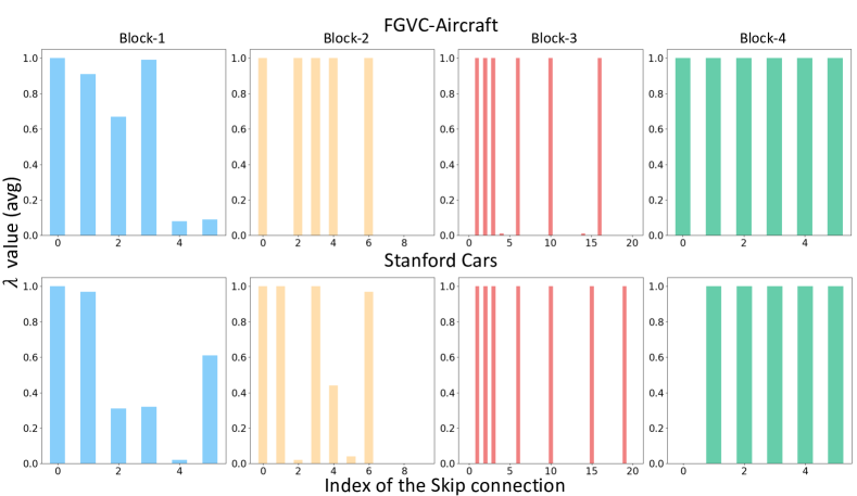
Figure 3: Despite not imposing a specific sparsity scheme, $\Delta$-Networks learns to select input-conditioned skip connections in a task-specific manner and zeros out some skip connections (especially in Blocks 2 and 3). Qualitative visualization of the weights (average) learned by the $\Delta$-Networks for all test samples of FGVC-Aircraft and Stanford Cars datasets, we use ResNeXt-50 as the base network and introduce four $\Delta$-modules in our $\Delta$-Networks, one for each block

9.2 Visualization of Learned Design Principles

We visualize the learned values of $\Lambda$ (weights assigned for the skip connection by the $\Delta$-module) for ResNet-18 on samples from three of the datasets we considered in our experiments.These visualizations are shown in Figures 4, 5, 6. These visualizations provide interesting insights that could be useful for architecture design in general. In particular, we note that: (i) In the initial modules, skip connections from the beginning of the block to the end of the block are sufficient, skip connections across blocks have a very less weight; and (ii) In the last module, all skip connections are required with each of them having a weight of 1. One common trend seen across all datasets is that weights for most skip connections in the last module of the network are always 1 consistently. This can also be observed in Figure 3.

Figure 4: Visualization of $\Lambda$ values on two samples of FGVC-Aircraft dataset [26] for ResNet-18 network

Figure 5: Visualization of $\Lambda$ values on two samples of Flowers-102 dataset [29] for ResNet-18 network

Figure 6: Visualization of $\Lambda$ values on two samples of Stanford-Cars dataset [22] for ResNet-18 network

References

- [1] Pre-trained models for Image Classification, 01 2023. https://huggingface.co/models?pipeline_tag=image-classification&sort=downloads.
- [2] Babak Ehteshami Bejnordi, Tijmen Blankevoort, and Max Welling. Batch-shaping for learning conditional channel gated networks. In International Conference on Learning Representations, 2020.
- [3] Nihar Bendre, Hugo Terashima Marín, and Peyman Najafirad. Learning from few samples: A survey. arXiv preprint arXiv: Arxiv-2007.15484, 2020.
- [4] Liang-Chieh Chen, Yukun Zhu, George Papandreou, Florian Schroff, and Hartwig Adam. Encoder-decoder with atrous separable convolution for semantic image segmentation. In Proceedings of the European Conference on Computer Vision (ECCV), September 2018.
- [5] Xinyang Chen, Sinan Wang, Bo Fu, Mingsheng Long, and Jianmin Wang. Catastrophic forgetting meets negative transfer: Batch spectral shrinkage for safe transfer learning. In H. Wallach, H. Larochelle, A. Beygelzimer, F. d'Alché-Buc, E. Fox, and R. Garnett, editors, Advances in Neural Information Processing Systems, volume 32. Curran Associates, Inc., 2019.
- [6] Nicola De Cao, Wilker Aziz, and Ivan Titov. Editing factual knowledge in language models. In Conference on Empirical Methods in Natural Language Processing (EMNLP), 2021.
- [7] M. Everingham, L. Van Gool, C. K. I. Williams, J. Winn, and A. Zisserman. The PASCAL Visual Object Classes Challenge 2007 (VOC2007) Results. http://www.pascal-network.org/challenges/VOC/voc2007/workshop/index.html.
- [8] Chrisantha Fernando, Dylan Banarse, Charles Blundell, Yori Zwols, David Ha, Andrei A. Rusu, Alexander Pritzel, and Daan Wierstra. PathNet: Evolution Channels Gradient Descent in Super Neural Networks. arXiv e-prints, page arXiv:1701.08734, Jan. 2017.
- [9] Chelsea Finn, Pieter Abbeel, and Sergey Levine. Model-agnostic meta-learning for fast adaptation of deep networks. In Proceedings of the 34th International Conference on Machine Learning, pages 1126–1135, 2017.
- [10] Xavier Glorot and Yoshua Bengio. Understanding the difficulty of training deep feedforward neural networks. In JMLR W&CP: Proceedings of the Thirteenth International Conference on Artificial Intelligence and Statistics (AISTATS 2010), volume 9, pages 249–256, May 2010.
- [11] Karan Goel, Albert Gu, Yixuan Li, and Christopher Re. Model patching: Closing the subgroup performance gap with data augmentation. In International Conference on Learning Representations, 2021.
- [12] Yunhui Guo, Honghui Shi, Abhishek Kumar, Kristen Grauman, Tajana Rosing, and Rogerio Feris. Spottune: Transfer learning through adaptive fine-tuning. In Proceedings of the IEEE/CVF Conference on Computer Vision and Pattern Recognition (CVPR), June 2019.
- [13] David Ha, Andrew M. Dai, and Quoc V. Le. Hypernetworks. In International Conference on Learning Representations, 2017.
- [14] Kaiming He, Xiangyu Zhang, Shaoqing Ren, and Jian Sun. Delving deep into rectifiers: Surpassing human-level performance on imagenet classification. In 2015 IEEE International Conference on Computer Vision (ICCV), pages 1026–1034, 2015.
- [15] Kaiming He, Xiangyu Zhang, Shaoqing Ren, and Jian Sun. Deep residual learning for image recognition. In Proceedings of the IEEE Conference on Computer Vision and Pattern Recognition (CVPR), June 2016.
- [16] Timothy Hospedales, Antreas Antoniou, Paul Micaelli, and Amos Storkey. Meta-learning in neural networks: A survey. IEEE transactions on pattern analysis and machine intelligence, 44(9):5149–5169, 2021.
- [17] Gao Huang, Zhuang Liu, Laurens van der Maaten, and Kilian Q. Weinberger. Densely connected convolutional networks. In Proceedings of the IEEE Conference on Computer Vision and Pattern Recognition (CVPR), July 2017.
- [18] Gao Huang, Yu Sun, Zhuang Liu, Daniel Sedra, and Kilian Q. Weinberger. Deep networks with stochastic depth. In Bastian Leibe, Jiri Matas, Nicu Sebe, and Max Welling, editors, Computer Vision – ECCV 2016, pages 646–661, Cham, 2016. Springer International Publishing.
- [19] Gabriel Ilharco, Mitchell Wortsman, Samir Yitzhak Gadre, Shuran Song, Hannaneh Hajishirzi, Simon Kornblith, Ali Farhadi, and Ludwig Schmidt. Patching open-vocabulary models by interpolating weights. In Advances in Neural Information Processing Systems, 2022.
- [20] Jiang Junguang, Baixu Chen, Fu Bo, and Mingsheng Long. Transfer-learning-library. https://github.com/thuml/Transfer-Learning-Library, 2020.
- [21] Zhi Kou, Kaichao You, Mingsheng Long, and Jianmin Wang. Stochastic normalization. In H. Larochelle, M. Ranzato, R. Hadsell, M. F. Balcan, and H. Lin, editors, Advances in Neural Information Processing Systems, volume 33, pages 16304–16314. Curran Associates, Inc., 2020.
- [22] Jonathan Krause, Michael Stark, Jia Deng, and Li Fei-Fei. 3d object representations for fine-grained categorization. In 4th International IEEE Workshop on 3D Representation and Recognition (3dRR-13), Sydney, Australia, 2013.
- [23] Xingjian Li, Haoyi Xiong, Hanchao Wang, Yuxuan Rao, Liping Liu, and Jun Huan. DELTA: DEEP LEARNING TRANSFER USING FEATURE MAP WITH ATTENTION FOR CONVOLUTIONAL NETWORKS. In International Conference on Learning Representations, 2019.
- [24] Zhizhong Li and Derek Hoiem. Learning without forgetting. In ECCV, 2016.
- [25] Wenqi Liu and Kun Zeng. SparseNet: A Sparse DenseNet for Image Classification. arXiv e-prints, page arXiv:1804.05340, Apr. 2018.
- [26] S. Maji, J. Kannala, E. Rahtu, M. Blaschko, and A. Vedaldi. Fine-grained visual classification of aircraft. Technical report, 2013.
- [27] M Jehanzeb Mirza, Jakub Micorek, Horst Possegger, and Horst Bischof. The norm must go on: dynamic unsupervised domain adaptation by normalization. In CVPR, 2022.
- [28] Eric Mitchell, Charles Lin, Antoine Bosselut, Chelsea Finn, and Christopher D Manning. Fast model editing at scale. In International Conference on Learning Representations (ICLR), 2021.
- [29] M-E. Nilsback and A. Zisserman. Automated flower classification over a large number of classes. In Proceedings of the Indian Conference on Computer Vision, Graphics and Image Processing, Dec 2008.
- [30] Adam Paszke, Sam Gross, Francisco Massa, Adam Lerer, James Bradbury, Gregory Chanan, Trevor Killeen, Zeming Lin, Natalia Gimelshein, Luca Antiga, Alban Desmaison, Andreas Köpf, Edward Yang, Zach DeVito, Martin Raison, Alykhan Tejani, Sasank Chilamkurthy, Benoit Steiner, Lu Fang, Junjie Bai, and Soumith Chintala. Pytorch: An imperative style, high-performance deep learning library. arXiv preprint arXiv: Arxiv-1912.01703, 2019.
- [31] Jo Plested and Tom Gedeon. Deep transfer learning for image classification: a survey. arXiv preprint arXiv: Arxiv-2205.09904, 2022.
- [32] Haoxuan Qu, Hossein Rahmani, Li Xu, Bryan Williams, and Jun Liu. Recent advances of continual learning in computer vision: An overview. arXiv preprint arXiv: Arxiv-2109.11369, 2021.
- [33] Alec Radford, Jong Wook Kim, Chris Hallacy, Aditya Ramesh, Gabriel Goh, Sandhini Agarwal, Girish Sastry, Amanda Askell, Pamela Mishkin, Jack Clark, Gretchen Krueger, and Ilya Sutskever. Learning transferable visual models from natural language supervision. In Marina Meila and Tong Zhang, editors, Proceedings of the 38th International Conference on Machine Learning, volume 139 of Proceedings of Machine Learning Research, pages 8748–8763. PMLR, 18–24 Jul 2021.
- [34] Colin Raffel. A call to build models like we build opensource software, 2021. https://cutt.ly/d8Jbq4J.
- [35] S-A Rebuffi, H. Bilen, and A. Vedaldi. Learning multiple visual domains with residual adapters. In NeurIPS, 2017.
- [36] Sylvestre-Alvise Rebuffi, Hakan Bilen, and Andrea Vedaldi. Efficient parametrization of multi-domain deep neural networks. In CVPR, 2018.
- [37] Shaoqing Ren, Kaiming He, Ross Girshick, and Jian Sun. Faster R-CNN: Towards real-time object detection with region proposal networks. In Advances in Neural Information Processing Systems (NIPS), 2015.
- [38] Marco Tulio Ribeiro and Scott Lundberg. Adaptive testing and debugging of nlp models. In Association for Computational Linguistics (ACL), 2022.
- [39] Marco Tulio Ribeiro, Tongshuang Wu, Carlos Guestrin, and Sameer Singh. Beyond accuracy: Behavioral testing of NLP models with CheckList. In Association for Computational Linguistics (ACL), 2020.
- [40] Shibani Santurkar, Dimitris Tsipras, Mahalaxmi Elango, David Bau, Antonio Torralba, and Aleksander Madry. Editing a classifier by rewriting its prediction rules. In Advances in Neural Information Processing Systems (NeurIPS), 2021.
- [41] Khadija Shaheen, Muhammad Abdullah Hanif, Osman Hasan, and Muhammad Shafique. Continual learning for real-world autonomous systems: Algorithms, challenges and frameworks. Journal of Intelligent & Robotic Systems, 105(1):1–32, 2022.
- [42] Jie Shao, Kai Hu, Changhu Wang, Xiangyang Xue, and Bhiksha Raj. Is normalization indispensable for training deep neural network? In H. Larochelle, M. Ranzato, R. Hadsell, M. F. Balcan, and H. Lin, editors, Advances in Neural Information Processing Systems, volume 33, pages 13434–13444. Curran Associates, Inc., 2020.
- [43] Samarth Sinha, Karsten Roth, Anirudh Goyal, Marzyeh Ghassemi, Zeynep Akata, Hugo Larochelle, and Animesh Garg. Uniform priors for data-efficient learning. In Proceedings of the IEEE/CVF Conference on Computer Vision and Pattern Recognition (CVPR) Workshops, pages 4017–4028, June 2022.
- [44] Anton Sinitsin, Vsevolod Plokhotnyuk, Dmitriy Pyrkin, Sergei Popov, and Artem Babenko. Editable neural networks. In International Conference on Learning Representations (ICLR), 2020.
- [45] Yisheng Song, Ting Wang, Subrota K Mondal, and Jyoti Prakash Sahoo. A comprehensive survey of few-shot learning: Evolution, applications, challenges, and opportunities. arXiv preprint arXiv: Arxiv-2205.06743, 2022.
- [46] Eric Tzeng, Judy Hoffman, Kate Saenko, and Trevor Darrell. Adversarial discriminative domain adaptation. In Proceedings of the IEEE Conference on Computer Vision and Pattern Recognition (CVPR), July 2017.
- [47] Jiachen Wang and Yingyun Yang. Sellf-adaptive weighted skip connections for image super-resolution. In 2020 International Conference on Culture-oriented Science Technology (ICCST), pages 192–197, 2020.
- [48] Xin Wang, Fisher Yu, Zi-Yi Dou, Trevor Darrell, and Joseph E. Gonzalez. Skipnet: Learning dynamic routing in convolutional networks. In Proceedings of the European Conference on Computer Vision (ECCV), September 2018.
- [49] Ross Wightman. Pytorch image models, 2019.
- [50] Zuxuan Wu, Tushar Nagarajan, Abhishek Kumar, Steven Rennie, Larry S Davis, Kristen Grauman, and Rogerio Feris. Blockdrop: Dynamic inference paths in residual networks. In CVPR, 2018.
- [51] Kaichao You, Zhi Kou, Mingsheng Long, and Jianmin Wang. Co-tuning for transfer learning. In H. Larochelle, M. Ranzato, R. Hadsell, M. F. Balcan, and H. Lin, editors, Advances in Neural Information Processing Systems, volume 33, pages 17236–17246. Curran Associates, Inc., 2020.
- [52] Hongyi Zhang, Yann N. Dauphin, and Tengyu Ma. Residual learning without normalization via better initialization. In International Conference on Learning Representations, 2019.
- [53] Jincheng Zhong, Ximei Wang, Zhi Kou, Jianmin Wang, and Mingsheng Long. Bi-tuning of Pre-trained Representations. arXiv e-prints, page arXiv:2011.06182, Nov. 2020.
- [54] Fuzhen Zhuang, Zhiyuan Qi, Keyu Duan, Dongbo Xi, Yongchun Zhu, Hengshu Zhu, Hui Xiong, and Qing He. A comprehensive survey on transfer learning. Proceedings of the IEEE, PP:1–34, 07 2020.