General Tasks and Extension-Based Proofs

Abstract.

The concept of extension-based proofs models the idea of a valency argument which is widely used in distributed computing. Extension-based proofs are limited in power: it has been shown that there is no extension-based proof of the impossibility of a wait-free protocol for $(n,k)$-set agreement among $n>k\geq 2$ processes. A discussion of a restricted type of reduction has shown that there are no extension-based proofs of the impossibility of wait-free protocols for some other distributed computing problems.

We extend the previous result to general reductions that allow multiple instances of tasks. The techniques used in the previous work are designed for certain tasks, such as the $(n,k)$-set agreement task. We give a necessary and sufficient condition for general colorless tasks to have no extension-based proofs of the impossibility of wait-free protocols, and show that different types of extension-based proof are equivalent in power for colorless tasks. Using this necessary and sufficient condition, the result about reductions can be understood from a topological perspective.

1. Introduction

In 1985, Fischer, Lynch, and Paterson (FLP, 85) proved one of the most important results in distributed computing : there is no deterministic wait-free protocol for the consensus task in the asynchronous message passing system. The key idea of their proof is called a valency argument, which proves the existence of an infinite execution that violates the wait-free requirement of the consensus task. Later, it was shown that this impossibility result can be extended to the shared memory model. This fundamental result led to the discovery of a totally new concept of computability power and the establishment of a highly active research area. In 1988, Biran, Moran and Zaks (BMZ, 88) provided a breakthrough result by introducing a graph-theoretic theorem that characterizes the general tasks that can be solved in a message passing model when one failure is allowed. However, this result was quite difficult to generalize to cases with more than one failure.

The $(n,k)$-set agreement task, which is a generalization of the consensus task, first proposed by Chaudhuri (Cha, 93), was independently solved by Borowsky and Gafni (BG93a, ), Herlihy and Shavit (HS, 99), and Saks and Zaharoglou (SZ, 00). In these works, topological techniques were used to study distributed computing. Borowsky and Gafni used a powerful simulation method that allows N-process protocols to be executed by fewer processes in a resilient way. The paper by Saks and Zaharoglou constructed a topological structure that captures processors’ local views of the whole system. The proof presented a relation between $(n,k)$-set agreement and Sperner’s lemma or the Brouwer fixed point theorem. The paper by Herlihy and Shavit introduced a more general formalism based on algebraic topology to discuss the computation in asynchronous distributed systems. They used topological structures, known as simplicial complexes, to model tasks and protocols. In this framework, they proved one of the most important theorems in distributed computing, the asynchronous computability theorem, which is a necessary and sufficient condition for a task to be solvable in shared memory model by a wait-free protocol. The impossibility result of the $(n,k)$-set agreement task was also proved using only combinatorial techniques in (AC, 11; AP, 12).

In (AAE⁺, 19), Alistarh, Aspnes, Ellen, Gelashvili and Zhu pointed out the differences between valency arguments and the combinatorial or topological techniques mentioned above. In those proofs using combinatorial or topological techniques, the existence of a bad execution is presented, but not explicitly constructed. In the original proof of the FLP result, an infinite execution can be obtained by extending an initial execution infinitely often. They generalized this type of proofs as extension-based proofs. An extension-based proof is defined as an interaction between a prover and a protocol that claims to solve a task. Initially, the prover only knows the initial configurations of the protocol. To obtain information about the protocol, the prover proceeds in phases. In each phase, the prover extends the set of configurations that were already reached during the interaction by submitting queries to the protocol. The prover wins if it discovers any safety or liveness violation. For example, the prover will win when it constructs infinite phases in the interaction. If there exists a prover that can win against any protocol that claims to solve a task, we say that this task has an extension-based impossibility proof. The proof of FLP impossibility result is an example of extension-based proofs. But this type of proofs does not appear to be a rather powerful tool. In the same paper, they showed that there are no extension-based proofs for the impossibility of a wait-free protocol for $(n,k)$-set agreement in the non-uniform iterated immediate snapshot (NIIS) model.

Will other tasks also have no extension-based impossibility proofs? One possible way to extend existing results is via reductions. A reduction from task $\mathcal{T}$ to task $\mathcal{S}$ is to use instances of task $\mathcal{S}$ to construct a protocol to solve task $\mathcal{T}$. Reductions from one problem to another have been widely studied to produce some new computability or complexity results from the known ones. A typical application of combinatorial topology in distributed computing is related to the renaming problem (CR, 08). To study the renaming lower bound, reductions among the renaming problem and several other problems, such as the $(n-1)$-set agreement task have been given. In distributed computing, reductions can be used to prove an impossibility result from an existing one. If reductions can be used to transform extension-based impossibility proofs from one task to another, we know that many other basic tasks in distributed computing will have no extension-based impossibility proofs. Brusse and Ellen (BE, 21) gave the first result about reductions: it is possible to transform extension-based impossibility proofs if the reduction is limited to the usage of only one instance, and extension-based proofs are augmented. They introduced augmented extension-based proofs, which generalize extension-based proofs by providing a new type of query. One of our goals is to answer the open question proposed in this paper, i.e. whether that restriction to one instance is unnecessary: If a task $\mathcal{T}$ reduces to a task $\mathcal{S}$ and $\mathcal{T}$ has an augmented extension-based proof of the impossibility of protocols, then $\mathcal{S}$ also has an augmented extension-based proof of the impossibility of protocols.

Since reductions can be used as a tool to generate new results, it is quite natural to try to draw a line between tasks that have extension-based impossibility proofs and those that do not. In Section 5, we prove a necessary and sufficient topological condition for a colorless task to have no extension-based impossibility proofs. The adversarial strategy in (AAE⁺, 19) is revised to accommodate general tasks. Finally, assignment queries are discussed to prove that different types of extension-based proofs are equivalent in power for colorless tasks.

This paper will be organized in this order: Section 2 is about related work. Since we will use the results of (HS, 99), the combinatorial topology and models used in this paper are briefly introduced in Section 3. Section 4 extends previous results on reductions. Section 5 uses more topological tools to study colorless tasks and gives a necessary and sufficient topological condition for a colorless task to have no extension-based proofs. We will also prove the equivalence of the power of different versions of extension-based proofs. Section 6 uses the results of Section 5 to discuss the reductions in a topological way. Finally, Section 7 summarizes our results and presents some potential extensions to our work.

2. Related work

2.1. NIIS model

The immediate snapshot (IS) object was introduced by Borowsky and Gafni in (BG93b, ). An IS object consists of an $(n+1)$ array and supports a single type of operation called a writeread operation, which writes a value to a single shared memory array cell and returns a snapshot of the array immediately following the write. It is the basic building block of the iterated immediate snapshot (IIS) model, first implicitly used by Herlihy and Shavit to prove sufficiency of the asynchronous computability theorem, and used as a new computation model by Borowsky and Gafni (BG, 97). In the execution of an IIS protocol, the sequence of IS objects is bounded and each process will terminate after accessing all IS objects in ascending or- der in the sequence. The IIS model was shown to have computational power equivalent to that of the standard shared memory model by providing an implementation of the IIS model from the shared memory model and vice versa.

Hoest and Shavit (HS, 97) used topological models and methods to analyze the asynchronous complexity of protocols. They introduced a new type of subdivision called the non-uniform chromatic subdivision and the NIIS model, a more flexible variant of iterated immediate snapshot (IIS) model that allows different processes to terminate after accessing different number of IS objects. The NIIS model assumes an unbounded sequence of IS objects. Therefore, each NIIS protocol is determined by a predicate $\tau$ from the local state of a process to a boolean value and a decision map $\delta$ from a terminated local state to output values. In the execution of an NIIS protocol $\mathcal{P}(\tau,\delta)$, each time a process completes a writeread operation, it checks whether it has reached the final state by applying the predicate $\tau$ to its local state variable. If the predicate $\tau$ returns true, the process executes a decide action and terminates. Otherwise, the predicate $\tau$ returns false, it continues to access the next IS object. Unlike the IIS model, the NIIS model permits executions of unbounded length, since it assumes an unbounded number of IS objects. Using the NIIS model, Hoest and Shavit presented the asynchronous complexity theorem showing that the time complexity of any asynchronous protocol is directly proportional to the level of non-uniform chromatic subdivisions necessary to construct a simplicial map from the input complex of a task to its output complex. It is known that the NIIS model is also computationally equivalent to the IIS model, and therefore, the standard shared memory model.

2.2. Extension-based proofs

In (AAE⁺, 19), Alistarh, Aspnes, Ellen, Gelashvili and Zhu formally defined the class of extension-based proofs that generalizes the impossibility proof techniques used in the FLP impossibility result. The proof of impossibility is modeled as an interaction between a prover and a NIIS protocol that claims to solve the task. The protocol is defined by a map $\Delta$ from the process states to the output values or a special value $NULL$. We use this notation $\Delta$ from (AAE⁺, 19), which is just a combination of the predicate and the decision map mentioned above. The prover asks queries to learn information about the protocol, such as the $\Delta$ values of states of processes in some reached configuration, in an effort to find a violation of the task specification, or construct an infinite schedule.

If there exists a prover that can defeat any protocol that claims to solve the task, we say that the task has an extension-based impossibility proof. But if we can define an adversary that can adaptively design a protocol according to the queries made by the prover such that any prover cannot win in the interaction, it is proved that there is no extension-based proof for the impossibility of the task. The main difficulty of research on extension-based proofs is to design an adversarial strategy such that no prover can win. The adaptive protocol constructed by the adversary will be referred to as an adversarial protocol as in (AAE⁺, 19).

As pointed out, extension-based proofs are too powerful for the IIS model, since a prover can perform an exhaustive search to finalize the output values of every reachable configuration. On the contrary, a protocol in the NIIS model can always defer its termination to leave some configurations undecided. In this paper, it will be assumed that each protocol that claims to solve the task is an NIIS protocol. A key observation is that the prover cannot learn all the information about the protocol during the interaction since it is only allowed to make finite queries. The adversary can terminate some configurations with different output values after the end of some phase depending on the schedule chosen by the prover. In (AAE⁺, 19) it is proved that after phase one of the interaction, the adversary can defeat any extension-based prover, since it can now partially specify a protocol for the reachable configurations in the later interaction. Note that not every configuration reached from some initial configuration is included here. This is why the adversarial protocol can exist while the task does not have a wait-free protocol. This observation is essential for understanding extension-based impossibility proofs for a general task, as we shall discuss later.

Three types of extension-based proofs (restricted extension-based proofs, extension-based proofs, augmented extension-based proofs) are defined in (AAE⁺, 19; BE, 21). These definitions share most settings, so we will first introduce the restricted extension-based proof, which is the weakest one. The interaction between the prover and a protocol proceeds in phases. In each phase $\varphi$ the prover starts with a finite schedule $\alpha(\varphi)$ and a set of configurations $\mathcal{A}(\varphi)$ reached from some initial configurations of the task by $\alpha(\varphi)$ which only differ in the input values of processes that are not in the schedule $\alpha$. The set of configurations reached in phase $\varphi$ is denoted by $\mathcal{A}^{{}^{\prime}}(\varphi)$ which is empty at the start of phase $\varphi$. The prover queries the protocol by choosing a configuration $C\in\mathcal{A}(\varphi)\bigcup\mathcal{A}^{{}^{\prime}}(\varphi)$ and a set of processes $P$ that are poised to update the same snapshot object in $C$. The protocol replies with the value of $\Delta$ of each process in $P$ in the resulting configuration $C^{{}^{\prime}}$ and the prover adds the configuration $C^{{}^{\prime}}$ to $\mathcal{A}^{{}^{\prime}}(\varphi)$. A chain of queries is a sequence of queries (finite or infinite) such that if $(C_{i},P_{i})$ and $(C_{i+1},P_{i+1})$ are consecutive queries in the chain, then $C_{i+1}$ is the configuration resulting from scheduling $P_{i}$ from $C_{i}$. The prover is allowed to construct finitely many chains of queries in a phase. If the prover does not find a violation or construct an infinite execution, it must end the phase by committing to an extension of $\alpha(\varphi)$ that will be used as the initial schedule in the next phase. If every process has terminated in all the configurations of $\mathcal{A}(\varphi)$, no extension will be possible, indicating the end of the interaction and failure of the prover. But if the prover manages to construct infinite phases, the prover wins.

Extension-based proofs allow for an additional type of query. The prover performs output queries by choosing a configuration $C\in\mathcal{A}(\varphi)\bigcup\mathcal{A}^{{}^{\prime}}(\varphi)$, a set of active processes $P$ that are poised to access the same snapshot object, and a value $y\in\{0,1,...,k\}$. If there is a $P$-only schedule from $C$ that results in a configuration in which a process in $P$ outputs $y$, the protocol will return the schedule. Otherwise, the protocol returns $NULL$. Augmented extension-based proofs adopt a more general definition called assignment queries. An assignment query consists of a configuration $C\in\mathcal{A}(\varphi)\bigcup\mathcal{A}^{{}^{\prime}}(\varphi)$, a set of processes $P$, and an assignment function $f$ from a subset $Q$ of $P$ to the output values. If there is a $P$-only schedule from $C$ that results in a configuration in which the output value of each process $q$ in $Q$ is $f(q)$, the protocol will return the schedule. Otherwise, the protocol will return $NULL$. It is shown that an output query $(C,P,y)$ can be simulated by a sequence of assignment queries $(C,P,f_{q})$ for each process $q$ in (BE, 21). Therefore, we will discuss only augmented extension-based proofs in subsequent sections.

2.3. Reductions in the IIS model

Herlihy, Kozlov and Rajsbaum (HKR, 13, Chapter 9.4.1) gave a definition of a reduction for tasks in the IIS model. If a task $\mathcal{T}$ reduces to another task $\mathcal{S}$, then there exists a protocol $\mathcal{P}_{0,k}$ that solves the task $\mathcal{T}$ and is equal to the composition

$$\mathcal{P}_{k-1,k}\cdot\mathcal{P}_{k-2,k-1}\cdots\mathcal{P}_{1,2}\cdot\mathcal{P}_{0,1}$$

of a sequence of protocols $\mathcal{P}_{i-1,i},1\leq i\leq k$, each of which is an immediate snapshot protocol or a protocol that solves the task $\mathcal{S}$. Previous work(BE, 21), however, used a restricted version of this definition in which only one instance $\mathcal{P}_{i-1,i}$ of this sequence is a protocol to solve the task $\mathcal{S}$.

In (BG93a, ; MRT, 06; GMRT, 09) it is shown that in a system made up of $n$ processes, $(n-1)$-set agreement, $(n-1)$-leader election, $(n-1)$-test&set and $(2p-\lceil\frac{p}{n-1}\rceil)$-renaming can be mutually transformed and therefore are equivalent. Similarly, there is a reduction from weak symmetry breaking to (2n-2)-set agreement and vice verse (HKR, 13, Chapter 12.2). But there is no reduction from set agreement to weak symmetry breaking (HKR, 13, Chapter 9.4.3). As noted in (BE, 21), there are reductions that require only one instance for these tasks. The restricted version of reductions in their paper is enough to prove the non-existence of extension-based proof for the above tasks. But some reductions use multiple instances, such as the reduction from weak symmetry breaking to $(n-1)$-set agreement which uses two instances of $(n-1)$-set agreement given by (GRH, 06).

3. Models

We give a description of our model, which largely follows that of Herlihy and Shavit(HS, 99) and the book by Herlihy, Kozlov and Rajsbaum(HKR, 13). Readers can refer to this book for more detailed information on distributed computing and topology.

Generally, $(n+1)$ sequential threads of control, called processes, communicate through asynchronous shared memory to solve decision tasks. A protocol is a distributed program to solve a task. A protocol is wait-free if it guarantees that every non-faulty process will terminate in a finite number of steps.

The input vector of a task is a vector of dimensions $(n+1)$ of objects that have the data type $D_{I}$ or a distinguished value $\perp$. The output vector is defined similarly. A vector $\vec{U}$ is called a prefix of vector $\vec{V}$ if for $0\leq i\leq n$, either $\vec{U}[i]=\vec{V}[i]$ or $\vec{U}[i]=\perp$. A set $V$ of vectors is prefix-closed if $\forall\vec{V}\in V$, each prefix of $\vec{V}$ is in $V$. Prefix-closed sets of $(n+1)$-dimensional vectors are used to characterize the legitimate sets of input and output value assignments. The set of input vectors is prefix-closed since any legitimate assignment of input values remains legitimate if fewer processes participate. By the same consideration, the set of output vectors is prefix-closed because any legitimate choice of output values remains legitimate if fewer processes decide. A general task specification is a relation $\Delta\subseteq I\times O$ that maps each input vector $\vec{I}$ to a nonempty subset of matching output vectors $\Delta(\vec{I})$. Therefore, a decision task $(\mathcal{I},\mathcal{O},\Delta)$ is defined as a tuple consisting of a prefix-closed set of input vectors, a prefix-closed set of output vectors, and a task specification $\Delta$ relating these two sets.

Objects, processes, and protocols are modeled as input/output $I/O$ automatons. An $I/O$ automaton is a nondeterministic automaton with a set of possible states, a set of input events, a set of output events, and a state transition relation defining all possible state changes by a given event. An execution of an $I/O$ automaton is an alternating sequence of states and enabled events, starting from some initial state. We adopt the definitions of (HS, 99): An object X is an automaton with input events $CALL\allowbreak(P,v,X,T)$ and output events $RETURN\allowbreak(P,v,X,T)$, where $P$ is a process id, $v$ is a value, $X$ is an object, and $T$ is a type. A process $P$ is an automaton with output events $CALL(P,v,X,T)$, $FINISH(P,v)$ and input events $RETURN(P,v,X,T)$ and $START(P,v)$. An operation is a pair of matching call and return events, that is, having the same type, name, and process id. A protocol $\mathcal{P}=\{{P_{0},...,P_{n};M}\}$ is the automaton composed by identifying in the obvious way the events for processes $P_{0},...,P_{n}$ and the memory $M$. During the execution of a protocol, the state of each process is called its local state. The local states of all processes together with the state of the memory are called the global state of the protocol. A protocol execution is well-formed if every process history has a unique start event, which precedes any call or return events, it alternates matching call and return events, and has at most one finish event.

A process is active at a point in an execution if it does not have a FINISH event. To capture the notion of fail-stop failures, we add to the process automaton a unique FAIL event after which there is no event. An active process is faulty at that point if it has a FAIL event. A protocol solves a task $(\mathcal{I},\mathcal{O},\Delta)$ in an execution if for all input vectors $\vec{I}$ corresponding to some participating processes, the output vector $\vec{O}$ is a prefix of some vector in $\Delta(\vec{I})$.

An (abstract) simplex is the set of all subsets of some finite set. An (abstract) simplicial complex is a finite collection of sets $S$, that is closed under subset: for any set $\sigma\in S$, if $\tau\subseteq\sigma$ , then $\tau\in S$. There is a natural geometric interpretation of an (abstract) simplicial complex which we will use later. A vertex $\vec{v}$ is a point in Euclidean space. A set $\{\vec{v}_{0},.....\vec{v}_{n}\}$ of vertices is affinely independent if and only if the vectors $\{\vec{v}_{1}-\vec{v}_{0},.....\vec{v}_{n}-\vec{v}_{0}\}$ are linearly independent. An n-simplex $S$ spanned by $\{\vec{v}_{0},.....\vec{v}_{n}\}$ is defined to be the set of all points x such that $x=\sum_{i=0}^{n}t_{i}\vec{v}_{i}$ where $\sum_{i=0}^{n}t_{i}=1$ and $t_{i}\geq 0$ for all $i$. Any simplex $T$ spanned by a subset of $\{\vec{v}_{0},.....\vec{v}_{n}\}$ is called a face of $S$. The faces of a simplex $S$ different from S are called the proper faces of $S$. A simplicial complex $\mathcal{K}$ is a collection of simplices closed under containment and intersection. That is, every face of every simplex of $\mathcal{K}$ is also a simplex of $\mathcal{K}$ and the intersection of two simplices of $\mathcal{K}$ is also a simplex of $\mathcal{K}$.

The dimension of a complex $\mathcal{K}$, denoted by dim($\mathcal{K}$), is the highest dimension of its simplices. A simplex $\sigma$ in $\mathcal{K}$ is a facet if it is not a proper face of any other simplex in $\mathcal{K}$. The dimension of $\mathcal{K}$ is the maximum dimension of any of its facets. If $\mathcal{L}$ is a subcollection of simplices in $\mathcal{K}$ that is also closed under containment and intersection, then $\mathcal{L}$ is a complex called a subcomplex of $\mathcal{K}$. A set of simplices of $\mathcal{K}$ of dimension at most $\ell$ is a subcomplex of $\mathcal{K}$, called $\ell{-}skeleton$ of $\mathcal{K}$, denoted by $skel^{\ell}(\mathcal{K})$. For example, elements of $skel^{0}(\mathcal{K})$ are just the vertices of $\mathcal{K}$.

There are two standard constructions that characterize the neighborhood of a vertex or a simplex: the star and the link. The star of a simplex $\sigma\in\mathcal{K}$, denoted as $St(\sigma,\mathcal{K})$ consists of all simplices $\tau$ that contain $\sigma$ and all simplices included in such a simplex $\tau$. The open star of a simplex $\sigma\in\mathcal{K}$, denoted as $St^{\circ}(\sigma,\mathcal{K})$ is the union of interiors of simplices that contain $\sigma$. The link of a simplex $\sigma\in\mathcal{K}$, denoted by $lk(\sigma,\mathcal{K})$, is the subcomplex of $\mathcal{K}$ consisting of all simplices in $St(\sigma,\mathcal{K})$ that do not share common vertices with $\sigma$.

Now, we define a way to join simplices. Let $S$ = $(\vec{s}_{0},\cdots,\vec{s}_{p})$ and $T$ = $(\vec{t}_{0},\cdots,\vec{t}_{q})$ be simplices such that the vertices of the combined set are affinely independent. Then the join of $S$ and $T$, denoted as $S*T$, is the simplex constructed from the set of vertices $(\vec{s}_{0},\cdots,\vec{s}_{p},\vec{t}_{0},\cdots,\vec{t}_{q})$.

Let $\mathcal{K}$ and $\mathcal{L}$ be complexes, possibly of different dimensions. A vertex map $\mu:skel^{0}(\mathcal{K})\rightarrow skel^{0}(\mathcal{L})$ is a map that takes vertices of $\mathcal{K}$ to vertices of $\mathcal{L}$. A vertex map is defined as a simplicial map if it carries each simplex of $\mathcal{K}$ to a simplex of $\mathcal{L}$. A simplicial map $\mu:\mathcal{K}\rightarrow\mathcal{L}$ is non-collapsing if it preserves dimension, that is, for all $S\in\mathcal{K}:dim(\mu(S))=dim(S)$. The most important non-collapsing simplicial map is the coloring of the n-dimensional complex $\mathcal{K}$ that labels the vertices of the complex so that no two neighboring vertices have the same color. A chromatic complex or colored complex $(\mathcal{K},\chi)$ is a complex $\mathcal{K}$ together with a coloring $\chi$. A simplicial map between colored complexes is color-preserving if it maps each vertex to a vertex of the same color.

Another important concept is the subdivision. A complex $\sigma(\mathcal{K})$ is a subdivision of $\mathcal{K}$ if

• Each simplex of $\sigma(\mathcal{K})$ is contained in a simplex of $\mathcal{K}$;

• Each simplex of $\mathcal{K}$ is the union of finitely many $\sigma(\mathcal{K})$.

The carrier of a simplex $S$ in a subdivision $\sigma(\mathcal{K})$, denoted $carrier(S,\allowbreak\mathcal{K})$, is the smallest simplex T of $\mathcal{K}$ such that $S$ is contained in $T$. A chromatic complex $(\sigma(\mathcal{K}),\chi_{\sigma(\mathcal{K})})$ is a chromatic subdivision of $(\mathcal{K},\chi_{\mathcal{K}})$ if $\sigma(\mathcal{K})$ is a subdivision of $\mathcal{K}$ and for all $S\in\sigma(\mathcal{K})$, $\chi_{\sigma(\mathcal{K})}(S)$ $\subseteq$ $\chi_{\mathcal{K}}(carrier(S,\mathcal{K}))$. The standard chromatic subdivision is the most important type of chromatic subdivision that we will use. Let $(\mathcal{K},\chi_{\mathcal{K}})$ be a chromatic simplicial complex. Its standard chromatic subdivision $Ch(\mathcal{K})$ is the simplicial complex of which the vertices have the form $(i,\sigma_{i})$, where $i\in[n]$, $\sigma_{i}$ is a non-empty face of $\sigma$, and $i\in\chi_{\mathcal{K}}(\sigma_{i})$. A $(k+1)$-tuple $(\sigma_{0},\cdots,\sigma_{k})$ is a simplex of $Ch(K)$ if and only if

• The tuple can be indexed so that $\sigma_{0}\subseteq\cdots\subseteq\sigma_{k}$;

• For $0\leq i,j\leq n$, if $i\in\chi_{\mathcal{K}}(\sigma_{j})$, then $\sigma_{i}\subseteq\sigma_{j}$.

and to make the subdivision chromatic, we define the coloring $\chi_{Ch(K)}$ as $\chi_{Ch(K)}(i,\sigma)=i$.

Earlier we define a decision task in terms of prefix-closed sets of input and output vectors. This set of all possible input or output vectors can be represented by a simplicial complex, called an input complex or an output complex, since by definition a simplicial complex is closed under containment. Each vertex $s$ of a simplex $S$ is labeled with a process id and a value which are denoted by $ids(s)$ and $vals(s)$, respectively. Given two simplicial complexes $\mathcal{K}$ and $\mathcal{L}$, a carrier map $\Phi$ from $\mathcal{K}$ to $\mathcal{L}$ takes each simplex $\sigma\in\mathcal{K}$ to a subcomplex $\Phi(\sigma)$ of $\mathcal{L}$ such that for all $\sigma,\tau\in\mathcal{K}$ such that $\sigma\subseteq\tau$, we have $\Phi(\sigma)\subseteq\Phi(\tau)$. The topological task specification corresponding to the task specification $\Delta$ is defined as a carrier map that carries each simplex of the input complex to a subcomplex of the output complex. We represent a decision task by a tuple $(\mathcal{I},\mathcal{O},\Phi)$ consisting of an input complex $\mathcal{I}$, an output complex $\mathcal{O}$, and a carrier map $\Phi$.

Like tasks, protocols can be defined in terms of combinatorial topology. A protocol is a triple $(\mathcal{I},\mathcal{P},\Xi)$ where $\mathcal{I}$ is the input complex, $\mathcal{P}$ is the protocol complex, and $\Xi$ is a carrier map called the execution map. A protocol $(\mathcal{I},\mathcal{P},\Xi)$ solves a task $(\mathcal{I},\mathcal{O},\Delta)$ if there is a simplicial map $\delta:\mathcal{P}\rightarrow\mathcal{O}$ such that $\delta*\Xi$ is carried by $\Delta$. Two protocols for the same set of processes can be composed: If we have two protocols $(\mathcal{I},\mathcal{P},\Xi)$ and $(\mathcal{I}^{{}^{\prime}},\mathcal{P}^{{}^{\prime}},\Xi^{{}^{\prime}})$ where $\mathcal{P}\subseteq\mathcal{I}^{{}^{\prime}}$, their composition is the protocol $(\mathcal{I},\mathcal{P}^{{}^{\prime\prime}},\Xi^{{}^{\prime\prime}})$, where $\Xi^{{}^{\prime\prime}}$ is the composition of $\Xi$ and $\Xi^{{}^{\prime}}$ and ${P}^{{}^{\prime\prime}}=\Xi^{{}^{\prime\prime}}(\mathcal{I})$. Similar compositions can be applied to two tasks or a protocol and a task.

In this paper, we are particularly interested in a subset of tasks called colorless tasks. It does not matter which process is assigned which input or which process chooses which output, only which sets of input values were assigned and which sets of output values were chosen. An input assignment for a set of processes $\Pi$ is a set of pairs $\{(P_{j},v_{j})|P_{j}\in\Pi,v_{j}\in V^{in}\}$, where each process $P_{j}\in\Pi$ appears exactly once, but the input values $v_{j}$ need not be distinct. A colorless input assignment is defined by an input assignment by discarding the process names. A colorless output assignment is defined by analogy with (colorless) input assignments. A colorless task is characterized by a set of colorless input assignments $I$, a set of colorless output assignments $O$, and a relation $\Delta$ that specifies, for each input assignment, which output assignments can be chosen. Colorless tasks are a central family of tasks in distributed computing. The consensus task, the set agreement task, and the approximate agreement task are examples of colorless tasks.

Herlihy and Shavit(HS, 99) proved the asynchronous computability theorem, a necessary and sufficient condition for a task to be solvable in the shared memory model.

Theorem 3.1 (Asynchronous computability theorem).

A decision task $(\mathcal{I},\mathcal{O},\Delta)$ has a wait-free protocol in the read-write memory model if and only if there exists a chromatic subdivision $\sigma$ of $\mathcal{I}$ and a color-preserving simplicial map $\mu:\sigma(\mathcal{I})\rightarrow\mathcal{O}$ such that for each simplex S in $\sigma(\mathcal{I})$, $\mu(S)\in\Delta(carrier(S,\mathcal{I}))$.

The asynchronous computability theorem transforms distributed computability problems into problems concerning static topological properties of topological spaces and is thus considered an important theorem in distributed computing.

In the proof of the asynchronous computability theorem, an important topological property is studied, called m-connectivity. Informally, a topological space is $m$-connected if it has no ”holes” in dimension $m$ and below. For example, a 0-connected complex is usually called connected if each pair of vertices is linked by a path. A 1-connected complex is usually called simply connected: Any closed path can be continuously deformed to a point. It is proved in (HKR, 13, Chapter 10.4) that for every wait-free IIS protocol and every input simplex $S^{m}$, the complex $\Xi(S^{m})$ is $m$-connected by applying the nerve graph and the nerve lemma. A set of simplicial complexes $\{\mathcal{K}_{i}|i\in I\}$ is called a cover for a simplicial complex $\mathcal{K}$ if $K=\cup_{i\in I}\mathcal{K}_{i}$. The nerve graph $\mathcal{N}(\mathcal{K}_{i}|i\in I)$ is defined as the simplicial complex whose vertices are the components $\mathcal{K}_{i}$. A set $\mathcal{J}$ of components $\{\mathcal{K}_{j}|j\in\mathcal{J}\}$ forms a simplex when the intersection $\cap_{j\in\mathcal{J}}\mathcal{K}_{j}$ is not empty. To compute the connectivity of a simplicial complex, we break it down into a cover, compute the connectivity of each component, and deduce the connectivity of the original complex from the connectivity of the components. ”Gluing” the components back together is formalized by the nerve lemma.

Lemma 3.2 (Nerve lemma).

Let $\{\mathcal{K}_{i}|i\in I\}$ be a cover for a simplicial complex $\mathcal{K}$. For any index set $\mathcal{J}\subseteq\mathcal{I}$, define $\mathcal{K}_{\mathcal{J}}=\cap_{j\in\mathcal{J}}\mathcal{K}_{j}$. Assume that for all $\mathcal{J}\subseteq\mathcal{I}$, $\mathcal{K}_{\mathcal{J}}$ is $(k-|\mathcal{J}|+1)$-connected or empty, then $\mathcal{K}$ is $k$-connected if and only if the nerve complex $\mathcal{N}(\mathcal{K}_{i}|i\in I)$ is $k$-connected.

We will analyze the detailed structure of the protocol complex and hence need some notations to simplify the statements. The notations from (HKR, 13, Chapter 10.2) will be adopted in later sections:

• Let $C\uparrow U$ denote the configuration obtained from $C$ by having the processes in $U$ simultaneously perform writeread operations in the next IS object.

• Let $\Xi(C)$ denote the complex of executions that can be reached starting from $C$, called the reachable complex from $C$.

• Let $(\Xi\downarrow U)(C)$ denote the complex of executions where, starting from C, the processes in $U$ halt without taking any further steps while the remaining processes complete the protocol.

For each configuration $C$, the reachable complexes $\{\Xi(C\uparrow U)|U\subseteq\Pi\}$, where $\Pi$ is the set of active processes in configuration $C$, cover $\Xi(C)$. This nerve complex has been shown to be a cone with an apex $\Xi(C\uparrow\Pi)$, and therefore n-connected. The nerve lemma implies that the protocol complex for an input simplex is also n-connected by induction on the dimension of the input simplex.

4. Reductions

In this section, we extend the proof in (BE, 21) to more general cases. We will use the notation in Section 2.3 to present reductions, although the tasks are now NIIS tasks rather than IIS tasks. Let $(\mathcal{R}_{1},\mathcal{R}_{2},....\mathcal{R}_{l},\mathcal{R}_{l+1})$ be a reduction from a task $\mathcal{T}$ to a task $\mathcal{S}$. Suppose that $\mathcal{P}_{T}$ is an augmented extension-based prover that can win against any protocol that claims to solve $\mathcal{T}$. Our goal is to construct an augmented extension-based prover $\mathcal{P}_{S}$ for the task $\mathcal{S}$ that can also win against any protocol that claims to solve $S$.

4.1. Composing NIIS protocols

The composition of NIIS protocols is much more complicated than the composition of IIS protocols, as processes can terminate after different rounds during the execution of some NIIS protocol. Processes accessing the same IS object in the composed protocol may be running different NIIS protocols. Let $A_{1}$ and $A_{2}$ be NIIS protocols such that each output from $A_{1}$ is a valid input for $A_{2}$. In (BE, 21), Brusse and Ellen provided an implementation of the composed protocol $A_{2}\cdot A_{1}$ using estimate vectors introduced by Borowsky and Gafni (BG, 97). An estimate vector is a potential output of a writeread operation of the snapshot object in the simulation of $A_{2}$. Each process locally maintains an infinite sequence of estimate vectors and updates its estimate vectors in the execution of the composed protocol $A_{2}\cdot A_{1}$. After a process has finished simulating $A_{1}$, it modifies its first estimate vector to include its output of $A_{1}$ for the simulation of $A_{2}$ and then tries to finalize it. To finalize its $k$-th estimate vector, for any $k\leq 1$, the process repeatedly performs a writeread operation on the next snapshot object in the composed protocol (to contain its first l estimate vectors), until the response from the scan satisfies certain conditions. When a process finalizes its $k$-th estimate vector, this vector will be used as the output of the writeread operation of the $k$-th IS object in the simulation of $A_{2}$. Note that it may take many rounds of the composed protocol for a process to finalize its current estimate vector, i.e. to take a step in the simulated execution. Based on the return values of its $k$-th estimate vector, the process may terminate its simulation of $A_{2}$ or modify its $(k+1)$-st estimate vector to include its new state in the simulation of A and continue to finalize its $(k+1)$-th estimate vector. A formal description is given in (BE, 21). An important property is that the composed protocol is wait-free if both $A_{1}$ and $A_{2}$ are wait-free.

Given an initial configuration $C_{1}$ of $A_{2}\cdot A_{1}$, their protocol simulates a schedule of $A_{1}$ from $C_{1}$, followed by a schedule of $A_{2}$, where outputs of the first schedule serve as inputs to the second schedule. Let $\alpha$ be a schedule of $A_{2}\cdot A_{1}$ from $C_{1}$. The restriction of $\alpha$ to $A_{1}$ is defined as the schedule $\alpha_{1}$ obtained from $\alpha$ by removing all the occurrences of each process after it has finished simulating $A_{1}$. Each process $p_{i}$ finishes its simulation of $A_{1}$ with output $y_{i}$ during the schedule $\alpha$ of $A_{2}\cdot A_{1}$ from $C_{1}$ if and only if $p_{i}$ terminates with output $y_{i}$ during the schedule $\alpha_{1}$ of $A_{1}$ from $C_{1}$.

Let $P$ be the set of processes that complete their simulation of $A_{1}$ during $\alpha$ from $C_{1}$ and, for each $p_{i}\in P$, let $y_{i}$ be its simulated output from $A_{1}$. Let $C_{2}$ be any initial configuration of $A_{2}$ in which each process $p_{i}\in P$ has input $y_{i}$. The estimate vectors finalized by processes correspond to the responses of writeread operations in some $P$-only schedule $\alpha_{2}$ of $A_{2}$ from $C_{2}$. Each process $p_{i}$ finishes its simulation of $A_{2}$ with output $z_{i}$ during the schedule $\alpha$ of $A_{2}\cdot A_{1}$ from $C_{1}$ if and only if $p_{i}$ terminates with output $z_{i}$ during the schedule $\alpha_{2}$ of $A_{2}$ from $C_{2}$. The restriction of $\alpha$ to $A_{2}$ is defined as the schedule $\alpha_{2}$. Note that the restriction to $A_{2}$ cannot be obtained from $\alpha$ by removing some occurrences similar to the restriction to $A_{1}$.

The composition of multiple NIIS protocols $A_{m}\cdots A_{2}\cdot A_{1}$ can be derived from the composition of two NIIS protocols. Each process will locally maintain $(m-1)$ infinite sequences of estimate vectors. Once a process finishes the simulation of $A_{i}$, for any $i\leq 1$, it will use the output value $z$ of $A_{i}$ as the initial value to start the simulation of $A_{i+1}$ (or terminate and output the value $z$ when $i=m$). Let $\alpha$ be a schedule of $A_{m}\cdots A_{2}\cdot A_{1}$ from some initial configuration $C_{1}$. The restriction of $\alpha$ to $A_{j},1\leq j\leq m$, denoted by $\alpha_{j}$, can be defined such that each process $p_{i}$ finishes the simulation of $A_{j}$ with output $z_{i}$ during schedule $\alpha$ of $A_{m}\cdots A_{2}\cdot A_{1}$ from $C_{1}$ if and only if $p_{i}$ terminates with output $z_{i}$ during schedule $\alpha_{j}$ of $A_{j}$ from some initial configuration $C_{j}$ of $A_{j}$ whose input values are the simulated outputs from $A_{j-1}$.

4.2. Reductions and extension-based proofs

As in the original proof, we can assume that tasks $\mathcal{R}_{1},\cdots,\mathcal{R}_{l},\allowbreak\mathcal{R}_{l+1}$ are all solvable in the IIS model, since the two models are equivalent in computability power. We denote these IIS protocols by $(B_{1},....B_{l},\allowbreak B_{l+1})$. The prover $\mathcal{P}_{S}$ knows everything about these protocols, such as the state of each process in any reachable configuration and how many rounds each protocol $B_{i}$ takes to terminate. If $A$ is some NIIS protocol that claims to solve the task $\mathcal{S}$, the composed protocol $(B_{l+1}\cdot A_{l}\cdot B_{l}\cdot A_{l-1}\cdots A_{1}\cdot B_{1})$ should solve $\mathcal{T}$ where each $A_{i}$ is the same protocol $A$. Note that each $A_{i}$ is an NIIS protocol and cannot be seen as an IIS protocol since extension-based proofs are too powerful for the IIS model. We will use estimate vectors to compose these protocols as described in Section 4.1.

The prover $\mathcal{P}_{S}$ will create $l$ instances of protocol $A$ and interact with each of them separately. Note that in the standard definition, an extension-based prover interacts with only one protocol. Here $\mathcal{P}_{S}$ is allowed to interact with multiple instances of $A$ and wins if it can win in the interaction with some instance. $\mathcal{P}_{S}$ will simulate an interaction between $\mathcal{P}_{T}$ and the composed protocol $(B_{l+1}\cdot A_{l}\cdot B_{l}\cdot A_{l-1}\cdots A_{1}\cdot B_{1})$. If the prover $\mathcal{P}_{T}$ submits a query in the simulation, the prover $\mathcal{P}_{S}$ will reinterpret this query as queries for some instances of protocol $A$ and will use the responses of the protocol instances and its knowledge about protocols $(B_{1},....B_{l},B_{l+1})$ to generate a response to the original query. To avoid confusion, we want to remind the readers that the composed protocol of NIIS protocols discussed in Section 4.1 is obtained by simulating the NIIS protocols sequentially. In this paragraph, we are talking about a simulated interaction between a prover and the composed protocol. Readers will have to distinguish them when we talk about simulation in subsequent discussions.

Let $\gamma$ be a schedule of the composed protocol $(B_{l+1}\cdot A_{l}\cdot B_{l}\cdot A_{l-1}\cdots A_{1}\cdot B_{1})$ from some initial configuration $C_{1}$. The restriction of $\gamma$ to a protocol $B_{i}$ or $A_{i}$ is defined using the general definition of restrictions in Section 4.1. An initial configuration $D_{i}$ of $A_{i}$ is defined as compatible with some configuration $C_{i}\gamma_{1i}$ of $B_{i}$ if the output value of every process that is terminated in $C_{i}\gamma_{1i}$ is the input value of the same process in $D_{i}$. An initial configuration $C_{i+1}$ of $B_{i+1}$ is defined as compatible with some configuration $D_{i}\gamma^{{}^{\prime}}_{i}$ of $A_{i}$ in the same way.

In the simulated interaction of $\mathcal{P}_{T}$, $\mathcal{P}_{S}$ maintains the following invariant: Suppose that $\mathcal{P}_{T}$ has reached the configuration $C=C_{1}\gamma$ of the composed protocol $(B_{l+1}\cdot A_{l}\cdot B_{l}\cdot A_{l-1}\cdots A_{1}\cdot B_{1})$. Let $\gamma_{1i}$ be the restriction of $\gamma$ to $B_{i}$, and let $\gamma_{i}^{{}^{\prime}}$ be the restriction of $\gamma$ to $A_{i}$. For each $1\leq i\leq l$, $\mathcal{P}_{S}$ has reached configuration $D_{i}\gamma_{i}^{{}^{\prime}}$ in interaction with the $i$-th $A$ instance, for some initial configuration $D_{i}$ of protocol $A$ compatible with $C_{i}\gamma_{1i}$, where $C_{i}$ is some initial configuration of $B_{i}$. And $C_{i+1}$ is compatible with $D_{i}\gamma_{i}^{{}^{\prime}}$. This invariant is a multiple instance generalization of the invariant in (BE, 21). Let $\psi$ denote the current phase of the simulated interaction and let $\phi_{i}$ denote the current phase of the $i$-th $A$ instance for each $1\leq i\leq l$. Similarly, for each interaction instance, the prover $\mathcal{P}_{T}$ maintains a finite schedule $\alpha_{i}(\phi_{i})$ for each phase $\phi_{i}$, which is the restriction of $\alpha(\psi)$ to $A_{i}$.

At the beginning of the simulation, the interaction between $\mathcal{P}_{T}$ and the composed protocol starts with an empty schedule and has reached the initial configurations of the composed protocol. For each $1\leq i\leq l$, the interaction between $\mathcal{P}_{S}$ and protocol $A_{i}$ also starts with an empty schedule and has reached initial configurations of $A_{i}$. Since every initial configuration of $B_{i}$ is compatible with every initial configuration of $A_{i}$, the invariant holds at the start of phase 1. We will discuss the strategy that the prover $\mathcal{P}_{S}$ will use in interactions with these $A$ protocol instances when $\mathcal{P}_{T}$ submits a query, submits an assignment query, or ends a phase in simulation.

4.2.1. Responding to queries

The proof of (BE, 21) has only discussed queries concerning one process. But the definition of restricted extension-based proofs allows concurrent update operations of a set of processes $P$ rather than just one process. Suppose that the prover $\mathcal{P}_{T}$ submits a query $(C,P)$ in phase $\psi$ of the simulated interaction. The prover $\mathcal{P}_{S}$ must respond with the configuration $C{P}$ resulting from scheduling $P$ from $C$ in the composed protocol. We can express the configuration $C$ as $C_{1}\alpha(\psi)\beta$ since the configuration $C$ has reached in phase $\psi$. The invariant holds before the query: Each interaction instance has reached some configuration $D_{i}\gamma_{i}^{{}^{\prime}}$ where $D_{i}$ is an initial configuration of $A_{i}$ compatible with $C_{i}\gamma_{1i}$. And $C_{i+1}$ is compatible with $D_{i}\gamma_{i}^{{}^{\prime}}$.

The processes in $P$ in the configuration $C$ of the composed protocol $(B_{l+1}\cdot A_{l}\cdot B_{l}\cdot A_{l-1}\cdots A_{1}\cdot B_{1})$ can be simulating the schedules of different protocols $A_{i}$ or $B_{i}$ as described in Section 4.1. This index $i$ can be calculated for each process in $P$ because the prover $\mathcal{P}_{T}$ can check if a process is still active in $A_{i}$ for any $i$ and know everything about protocol $B_{i}$. If some process $p$ in $P$ finalizes its current estimate vector (or simulates the first protocol $B_{1}$) after accessing the new IS object, $p$ takes a step in its simulated protocol. Otherwise, the simulated execution will not proceed and the values of $\gamma_{1i}$ and $\gamma_{i}^{{}^{\prime}}$ will not change. Let $P^{{}^{\prime}}$ be the set of processes in $P$ that will take a step in some simulated protocol $A_{i}$ or $B_{i}$. Let $P^{{}^{\prime}}_{k}$ be processes in $P^{{}^{\prime}}$ that are poised to access the $k$-th simulated IS object. There are a number of cases, depending on what steps processes in $P^{{}^{\prime}}_{k}$ take in configuration $C$.

If processes in $P^{{}^{\prime}}_{k}$ simulate some $B_{i}$ and do not execute the last step, they still simulate $B_{i}$ after taking a step. Let $C_{n}$ be the configuration resulting from scheduling $P^{{}^{\prime}}_{k}$ from $C_{i}\gamma_{1i}$. The prover $\mathcal{P}_{S}$ can return the states of $P^{{}^{\prime}}_{k}$ in $C_{n}$ to $\mathcal{P}_{T}$ using its knowledge of $B_{i}$. No more processes terminate in the simulated execution of $B_{i}$, and $D_{i}$ is compatible with $C_{n}$. The invariant continues to hold.

If processes in $P^{{}^{\prime}}_{k}$ simulate some $B_{i}$ and execute the last step, each process will output a value and terminate in the simulation of $B_{i}$ since $B_{i}$ is assumed to be an IIS protocol. Let $C_{n}$ be the configuration resulting from scheduling $P^{{}^{\prime}}_{k}$ from $C_{i}\gamma_{1i}$. $\mathcal{P}_{S}$ can return the states of $P^{{}^{\prime}}_{k}$ in $C_{n}$ to $\mathcal{P}_{T}$. $D_{i}$ has to be changed since more processes have been terminated in the simulation of $B_{i}$. We can choose a new initial configuration $D_{i}^{{}^{\prime}}$ of $A_{i}$ in which each newly terminated process $p$ will use the output of $B_{i}$ as input and every other process has the same input as $D_{i}$. The new initial configuration $D_{i}^{{}^{\prime}}$ is compatible with $C_{n}$. The newly terminated processes do not appear in $\gamma_{i}^{{}^{\prime}}$, so $\gamma_{i}^{{}^{\prime}}$ is a valid schedule from the new initial configuration $D_{i}^{{}^{\prime}}$. The invariant holds in this case.

Suppose that processes in $P^{{}^{\prime}}_{k}$ simulate some $A_{i}$. The prover $\mathcal{P}_{S}$ can submit the query $(D_{i}\gamma_{i}^{{}^{\prime}},P^{{}^{\prime}}_{k})$ to the protocol $A_{i}$ and return the response to $\mathcal{P}_{T}$. If no process terminates in the simulation, the invariant holds since $\gamma_{i}^{{}^{\prime}}P^{{}^{\prime}}_{k}$ is the new restriction to $A_{i}$ and will not change the initial values of active processes in $A_{i}$ or $B_{i+1}$. Otherwise, some processes in $P^{{}^{\prime}}_{k}$ terminate in the simulation of $A_{i}$, and the initial configuration $C_{i+1}$ of $B_{i+1}$ must be changed. For each terminated process $p$ in $P^{{}^{\prime}}_{k}$, the input value for $B_{i+1}$ is the output value of $D_{i}\gamma_{i}^{{}^{\prime}}$. Let $D_{n}$ be the configuration resulting from scheduling $P^{{}^{\prime}}_{k}$ from $D_{i}\gamma^{{}^{\prime}}_{i}$. The new initial configuration $C_{i+1}$ of $B_{i+1}$ is compatible with $D_{n}$. The invariant still holds, since the simulation of each $A_{i}$ is not affected.

The prover $\mathcal{P}_{S}$ may submit multiple queries $(D_{i}\gamma_{i}^{{}^{\prime}},P^{{}^{\prime}}_{k})$ for different $k$ to some protocol $A_{i}$. Operations on different simulated IS objects will not affect each other. Therefore, submitting these queries in different orders will not change the response of each query and the internal variants(such as the set of configurations reached in phase $\phi_{i}$) of the interaction between $\mathcal{P}_{S}$ and $A_{i}$.

4.2.2. Responding to assignment queries

Suppose that the prover $\mathcal{P}_{T}$ submits an assignment query $(C,P,f)$ in phase $\psi$ of the simulated interaction, the prover $\mathcal{P}_{S}$ has to reply whether there exists a $P$-only schedule from $C$ to a configuration $C_{d}$ in which the output value of each process $q$ in $Q$ is $f(q)$. We will say that this configuration $C_{d}$ satisfies the requirement of $f$. Since $\mathcal{P}_{T}$ will not reach any new configuration to respond to assignment queries, the invariant will continue to hold.

By the invariant, for $1\leq i\leq l$, $\mathcal{P}_{S}$ has reached the configuration $D_{i}\gamma_{i}^{{}^{\prime}}$ in the $i$-th interaction with $A$, for some initial configuration $D_{i}$ of protocol $A_{i}$ compatible with $C_{i}\gamma_{1i}$, where $\gamma_{1i}$ is the restriction of $\gamma$ to $B_{i}$ and $\gamma_{i}^{{}^{\prime}}$ is the restriction of $\gamma$ to $A_{i}$. And $C_{i+1}$ is compatible with $D_{i}\gamma_{i}^{{}^{\prime}}$.

The prover $\mathcal{P}_{S}$ will treat all protocols $B_{i}$ and $A_{i}$ as black boxes that allow assignment queries. This is possible for each $A_{i}$ since the prover $\mathcal{P}_{S}$ can submit the same assignment query to protocol $A_{i}$. The prover $\mathcal{P}_{S}$ knows everything about the protocol $B_{i}$, so assignment queries are also possible for $B_{i}$. We regard protocols of both types as black boxes to simplify our proof. The prover $\mathcal{P}_{S}$ will compute a set of assignment queries from the configuration $C$ to the input complex of each protocol, denoted by $F_{i}$. This is done by tracing back from the $(i+1)$-th protocol to the $i$-th protocol to compute $F_{i}$ from $F_{i+1}$. We define $F_{2l+2}$ as the original query $(C,P,f)$.

First, $\mathcal{P}_{S}$ computes $F_{2l+1}$, which is the set of all possible assignment queries before the protocol $B_{l+1}$. Let $C_{c}$ be some initial configuration of the protocol $B_{l+1}$ compatible with $D_{i}\gamma^{{}^{\prime}}_{l}$, where there is a $P$-only schedule $\beta$ from $C_{c}\gamma^{{}^{\prime}}$ to a configuration that satisfies the requirement of $f$. Let $P^{{}^{\prime}}$ denote the set of processes obtained from $P$ by removing the processes that appear in $\gamma^{{}^{\prime}}$.

Now we will prove that there exists a $P^{{}^{\prime}}$-only schedule to some $C_{c}\gamma^{{}^{\prime}}$ if and only if there exists a $P$-only schedule to some output configuration that satisfies $f$. If there is a $P^{{}^{\prime}}$-only schedule $\beta^{{}^{\prime}}$ from $C$ to a configuration $C_{c}\gamma^{{}^{\prime}}$, we can see that there is a $P$-only schedule $\beta^{{}^{\prime}}\beta$ from $C$ to a configuration that satisfies the requirement of the function $f$. On the other hand, if there is a $P$-only schedule $\beta^{{}^{\prime\prime}}$ from $C$ to some configuration $C_{d}$ that satisfies the requirement of $f$, $C_{d}$ can be seen as an output configuration of the last protocol $B_{l+1}$. Therefore, there exists an initial configuration $C_{c}$ of the protocol $B_{l+1}$ compatible with $D_{i}\gamma^{{}^{\prime}}_{l}$, and there is a $P$-only schedule $\beta$ from $C_{c}\gamma^{{}^{\prime}}$ to a configuration that satisfies the requirement of $f$. Consider the schedule $\beta_{c}$ from $C$ to $C_{c}\gamma^{{}^{\prime}}$. The restriction of $\beta_{c}$ to $B_{i}$ and $A_{i}$ for $1\leq i\leq l$ will contain only the processes in $P^{{}^{\prime}}$. But this is not true for $\beta_{c}$ because some process in $P-P^{{}^{\prime}}$ may appear in $\beta_{c}$, but does not take a step in the simulation. A $P^{{}^{\prime}}$-only schedule of the composed protocol can be constructed by removing all occurrences of processes in $P^{{}^{\prime}}$ from $\beta_{c}$, so that its restriction to $B_{i}$ and $A_{i}$ for $1\leq i\leq l$ is the same as $\beta^{{}^{\prime\prime}}$. Therefore, there is a $P^{{}^{\prime}}$-only schedule of the composed protocol from $C$ to $C_{c}\gamma^{{}^{\prime}}$.

For each such initial configuration $C_{c}$ we can submit an assignment query $(C,P^{{}^{\prime}},f^{{}^{\prime}})$ to the composed protocol $(A_{l}\cdot B_{l}\cdot A_{l-1}\cdots A_{1}\cdot B_{1})$ in which $f^{{}^{\prime}}$ is defined as a function from the processes in $P^{{}^{\prime}}$ to their output values in configuration $C_{c}$. If a $P^{{}^{\prime}}$-only schedule is returned, the prover $\mathcal{P}_{S}$ can return a $P$-only schedule to the prover $\mathcal{P}_{T}$. Otherwise, the prover $\mathcal{P}_{S}$ has to return $NULL$. $F_{2l+1}$ consists of all these assignment queries $(C,P^{{}^{\prime}},f^{{}^{\prime}})$.

The tracing back continues: Suppose that $F_{i+1}$ is already calculated. For each assignment query $(C,P^{{}^{\prime}},f^{{}^{\prime}})$ in $F_{i+1}$, the prover $\mathcal{P}_{S}$ will compute each initial configuration $C_{c}$ that is compatible with the input values of the active vertices in the current protocol, and there should be a $P^{{}^{\prime}}$-only schedule $\beta$ from $C_{c}\gamma^{{}^{\prime}}$ to a configuration that satisfies the function $f^{{}^{\prime}}$, where $\gamma^{{}^{\prime}}$ is the restriction of $\gamma$ to the current protocol. Let $P^{{}^{\prime\prime}}$ denote the set of processes obtained from $P^{{}^{\prime}}$ by removing the processes in $\gamma^{{}^{\prime}}$. For each initial configuration $C_{c}$, there is an assignment query $(C,P^{{}^{\prime\prime}},f^{{}^{\prime\prime}})$ in which $f^{{}^{\prime\prime}}$ is defined to be a function from the processes in $P^{{}^{\prime\prime}}$ to the values in configuration $C_{c}$. As proved in the above example, there is a $P^{{}^{\prime\prime}}$-only schedule from configuration $C$ to configuration $C_{c}\gamma^{{}^{\prime}}$ if and only if there is a $P^{\prime}$-only schedule for assignment query $(C,P^{{}^{\prime}},f^{{}^{\prime}})$. $F_{i}$ consists of all these assignment queries $(C,P^{{}^{\prime\prime}},f^{{}^{\prime\prime}})$.

This procedure will end when $P^{{}^{\prime\prime}}$ is empty. If there exists an assignment query in $F_{i}$, there exists a $P$-only schedule from $C$ to some configuration satisfying the requirement of $f$. Otherwise, the prover $\mathcal{P}_{S}$ returns $NULL$.

4.2.3. Ending phases

Suppose that the prover $\mathcal{P}_{T}$ decides to end its current phase $\psi$ by choosing a configuration $C=C_{0}\alpha(\psi)\beta$ of the composed protocol $(B_{l+1}\cdot A_{l}\cdot B_{l}\cdot A_{l-1}\cdots A_{1}\cdot B_{1})$. By the invariant, $\mathcal{P}_{S}$ has reached configuration $D_{i}\gamma_{i}^{{}^{\prime}}$ in the $i$-th interaction with protocol $A$, for some initial configuration $D_{i}$ of protocol $A$, where $\gamma_{i}^{{}^{\prime}}$ is the restriction of $\gamma$ to $A_{i}$.

For those $A$ instances in which no simulation is performed, the prover $\mathcal{P}_{S}$ does nothing, and the invariant continues to hold. For a protocol instance $A_{i}$ in which at least one process has taken a simulation step during the schedule $\beta$ of the composed protocol, the prover $\mathcal{P}_{T}$ has reached the configuration $D_{i}\gamma_{i}^{{}^{\prime}}$. The prover $\mathcal{P}_{S}$ ends phase $\phi_{i}$ by choosing configuration $D_{i}\gamma_{i}^{{}^{\prime}}$ and set $\alpha_{i}(\phi_{i}+1)=\gamma_{i}^{{}^{\prime}}$.

4.2.4. The prover $\mathcal{P}_{S}$ will win

The prover $\mathcal{P}_{T}$ will finally win in the simulated interaction with the composed protocol $(B_{l+1}\cdot A_{l}\cdot B_{l}\cdot A_{l-1}\cdots A_{1}\cdot B_{1})$. We will analyze all possible circumstances and show that $\mathcal{P}_{S}$ will win against one of the instances of the protocol $A$.

The first case is that the prover $\mathcal{P}_{T}$ finds a violation of the task specification of $\mathcal{T}$, and let $C$ denote the configuration with incorrect output values. For example, the processes in $C$ output different values when $\mathcal{T}$ is the consensus task. By the invariant, the prover $\mathcal{P}_{S}$ has reached configuration $D_{i}\gamma_{i}^{{}^{\prime}}$ in the $i$-th interaction with $A$, for some initial configuration $D_{i}$ of protocol $A$. Suppose that for each interaction instance, the output values of the processes in $D_{i}\gamma_{i}^{{}^{\prime}}$ satisfy the task specification of $\mathcal{S}$. The output values in configuration $C$ will satisfy the task specification of $\mathcal{T}$ as $\mathcal{T}$ reduces to $\mathcal{S}$, which is a contradiction. Therefore, there exists an interaction with some $A_{i}$ that reaches a configuration with incorrect output values. The prover $\mathcal{P}_{S}$ has found a violation of the task specification and wins against the protocol $A$.

The second case is that the prover $\mathcal{P}_{T}$ constructs an infinite chain of queries in the interaction. Each protocol $B_{i}$ is wait-free, so an infinite schedule is not possible in it. Estimation vectors will not cause an infinite schedule of the composed protocol, as proved in (BE, 21). Therefore, there must be an interaction with some $A$ instance in which the prover $\mathcal{P}_{S}$ also constructs an infinite chain of queries. In this situation, the prover $\mathcal{P}_{S}$ wins.

The last case is that the prover $\mathcal{P}_{T}$ constructs infinite phases in the simulation. By definition, $\mathcal{P}_{T}$ can submit finitely many queries or assignment queries in one phase. Each time the prover $\mathcal{P}_{T}$ ends its phase by choosing a schedule $\beta$, at least one step is taken by some set of processes. Since each protocol $B_{i}$ is wait-free, the prover $\mathcal{P}_{T}$ can only end a finite number of phases by simulating only the $B$ protocols. For other phases, there must be some protocol $A_{i}$ that will make progress and, therefore, end its current phase after the prover $\mathcal{P}_{T}$ ends a finite number of phases. The number of $A$ protocol instances is finite, so there must be an interaction with some $A$ instance in which the prover $\mathcal{P}_{S}$ also constructs infinite phases. The prover $\mathcal{P}_{S}$ still wins.

We summarize the above results as a theorem.

Theorem 4.1.

If a task $\mathcal{T}$ reduces to a task $\mathcal{S}$ using multiple instances of task $\mathcal{S}$ and there is an augmented extension-based proof of the impossibility of solving the task $\mathcal{T}$, then there is an augmented extension-based proof of the impossibility of solving the task $\mathcal{S}$.

This result allows us to deduce the non-existence of augmented extension-based impossibility proofs for many tasks using existing reductions, although many important results are already available when reductions are restricted (BE, 21). Some reductions, such as the one introduced in (GRH, 06), do not have to be excluded because multiple instances of task $\mathcal{S}$ are used.

5. A necessary and sufficient condition to have no extension-based impossibility proofs

The $(n,k)$-set agreement task is the first task that has been shown to have no extension-based impossibility proofs. As shown in (AAE⁺, 19), the adversary will pretend to have a protocol for the $(n,k)$-set agreement task during phase 1 of the interaction. But after the prover chooses a schedule at the end of phase 1, the adversary can assign a valid value to each undefined vertex that can be reached. In other words, the adversary has a restricted protocol that satisfies the task specification of the $(n,k)$-set agreement after phase 1.

For a general task $(\mathcal{I},\mathcal{O},\Delta)$, the task specification $\Delta$ maps each input vector to a nonempty subset of output vectors. Let $s$ be some simplex in a subdivision of $\mathcal{I}$, an output configuration of $s$ satisfies the carrier map $\Delta$(or satisfies the task specification) if for any subsimplex $s^{{}^{\prime}}$ of $s$, the output vector of $s^{{}^{\prime}}$ is in $\Delta(carrier(s^{{}^{\prime}},I))$. A protocol satisfies the carrier map $\Delta$(or satisfies the task specification) if each output configuration does.

We will call it finalization if the adversary can construct a restricted protocol after a certain phase $t$, that is, assign a value to each vertex of some subdivision of all reachable configurations in later phases satisfying the carrier map $\Delta$. If the adversary can always finalize after some phase $t$ without violating the task specification or allowing an infinite chain of queries in the previous interaction, the adversary will win against any extension-based prover. We can argue that the prover cannot win. A violation of the task specification or an infinite chain of queries is not possible before finalization by the assumption and is not possible after finalization since there will be a constructed protocol. Infinite phases cannot be constructed, as the prover will choose a configuration at the end of some phase after $t$ in which every process has terminated. If the adversary cannot finalize after the prover chooses some configuration $\beta_{t}$ at the end of phase $t$, then there must be a reachable configuration in which not all processes are terminated. There is a configuration in $\mathcal{A}^{{}^{\prime}}(t)$ in which some processes are not terminated. If, in every configuration in $\mathcal{A}(t+1)$, every process has terminated, then the prover loses and the interaction ends. By choosing the configuration $\beta_{t}$ to end in each phase $t$, the prover can construct infinite phases. A tight connection between the finalization and the interaction result has been shown, and we will discuss the conditions for the adversary to finalize in the following sections.

Let $\alpha_{t}$ be the schedule chosen by the prover at the end of phase $t$. $\alpha_{t}$ is an ordered sequence of subsets of processes that are poised to perform writeread operations on the same IS object. Such a subset of processes is called a process set in our subsequent discussions. So $\alpha_{t}$ contains at least $t$ process sets that the adversary will use to build a protocol for a subcomplex of some subdivision of $\mathcal{I}$.

5.1. General tasks with partial input information

In this section, we give a necessary condition for the finalization after phase 1. At that time, the prover has chosen a configuration $C^{{}^{\prime}}$ $\in$ $\mathcal{A}^{{}^{\prime}}(1)$ and let $\alpha^{{}^{\prime}}$ denote the schedule from some initial configuration $C\in\mathcal{A}(1)$ to $C^{{}^{\prime}}$. All possible configurations in phase 2, denoted by $\mathcal{A}(2)$, are the configurations reached by performing $\alpha^{{}^{\prime}}$ from the initial configurations that differ only from $C$ by input values of processes not in the schedule $\alpha^{{}^{\prime}}$.

Consider the configuration reached from the same initial configuration $C$ by the schedule $\alpha^{{}^{\prime\prime}}$ consisting only of the first process set $U$ in $\alpha^{{}^{\prime}}$, if we can still finalize $\Delta$ in this case, then there must be a finalization for the original schedule $\alpha^{{}^{\prime}}$ because all the configurations reached from $\alpha^{{}^{\prime}}$ are contained in the configurations reached from $\alpha^{{}^{\prime\prime}}$. Therefore, we can assume without loss of generality that the schedule $\alpha^{{}^{\prime}}$ contains only one process set.

If the adversary can finalize after phase 1, then for each initial configuration $C$ and each process set $U$, we can assign output values to the vertices in $\Xi(C\uparrow U)$. Each n-simplex represents a reachable configuration in which each process has a valid output value. In proof of non-existence of extension-based impossibility proofs for $(n,k)$-set agreement, this is simply done by setting $\Delta(v)=a$ ($a$ is the input value of some process in $U$) for each undefined vertex. At most 2 different values will be output in any output configuration. Let $Q(C,U)$ denote the subcomplex of $Ch(C)$ representing the configurations reached from $C\uparrow U$. Let $Input(U,V)$, where $U$ is an ordered set of processes and $V$ is an ordered set of input values, denote $\sum Q(C,U)$ where $C$ is an input configuration such that the $i$-th process in $U$ will have the $i$-th input value in $V$ for each $i$. Note that the input configuration $C$ is not unique. We will slightly abuse the notation by saying that there exists a restricted protocol for $Input(U,V)$ if there exists a chromatic subdivision of $Input(U,V)$ and a color-preserving simplicial map $\mu:\sigma(Input(U,V))\rightarrow O$ such that for each simplex $S$ in $\sigma(Input(U,V))$, $\mu(S)\in\Delta(carrier(S,I))$. A necessary condition for the finalization after phase 1 is that there is a restricted protocol for each $Input(U,V)$. This is not a sufficient condition, since the output values of some configurations in $\Xi(C\uparrow U)$ can be determined in phase 1.

Before any process not in $U$ can perform an operation, processes in $U$ will writeread the first IS object concurrently using their input values. Therefore, each process will read the input values of all processes in $U$ from the return value of the operation on the first IS object. We define some notation. Given a simplex $\tau$ in the input complex $\mathcal{I}$, we divide all n-simplices in the output complex $\mathcal{O}$ into different sets labeled by the output values of processes in $\tau$. The output complex restricted to the input simplex $\tau$, denoted by $\mathcal{O}_{\tau}$, is defined as the sets whose label satisfies the carrier map $\Delta$. In other words, for each subsimplex $\tau^{{}^{\prime}}\in\tau$, its output vector is contained in $\Delta(\tau^{{}^{\prime}})$. Therefore, we can iterate all sets as $\mathcal{O}_{\tau}=\{\mathcal{O}_{\tau}^{0},\mathcal{O}_{\tau}^{1},\cdots\mathcal{O}_{\tau}^{m}\}$ by associating each label with a unique index. Let $P$ be the ids of $\tau$, which is the set of processes. The notation $\mathcal{O}_{\tau}\backslash\tau$ is defined as a simplicial complex generated by removing vertices whose ids are in $P$ from $\mathcal{O}_{\tau}$.

Lemma 5.1.

For a general task$(\mathcal{I},\mathcal{O},\Delta)$, there exists a protocol when the first process set in the schedule is determined if and only if for each n-simplex $\sigma\in\mathcal{I}$, $\forall\tau\subset\sigma$, there exists $\mathcal{O}_{\tau}^{i}$ for some $0\leq i\leq m$, such that the task $(lk(\tau,\mathcal{I})$, $\mathcal{O}_{\tau}^{i}\backslash\tau$, $\Delta_{\tau})$ has a protocol, where $\Delta_{\tau}$ carries a simplex $\tau^{{}^{\prime}}$ $\subseteq$ $lk(\tau,\mathcal{I})$ to the complex $\Delta(\tau^{{}^{\prime}}*\tau)\backslash\tau$, which is generated from $\Delta(\tau^{{}^{\prime}}*\tau)$ by removing vertices whose ids are in $ids(\tau)$.

Proof.

We first prove necessity. Let $U$ be the set of processes in $\tau$. Suppose that there is a protocol when the first process set is determined, consider the execution in which only processes in $U$ run and decide. The output simplex of $U$ must be in $\Delta(\tau)$, and therefore be associated with some index $i$. We denote this configuration by $C_{1}$. At this time, active processes are those not in $ids(\tau)$. Let all the remaining processes run and decide. The output values of the processes not in $U$ will be simplices in $\mathcal{O}_{\tau}^{i}\backslash\tau$.

Let $C_{0}$ be an initial configuration of the protocol. For processes not in $U$, the configuration $C_{1}$ will not provide more information than the configuration $C_{0}$ since the input values of all processes in $\tau$ are already known. For any schedule $\alpha$ from $C_{0}$ consisting of processes not in $\tau$, we can return the configuration reached from $C_{1}$ by $\alpha$. Then we have constructed a protocol for the task $(lk(\tau,\mathcal{I})$, $\mathcal{O}_{\tau}^{i}\backslash\tau$, $\Delta_{\tau})$.

Next, we prove sufficiency. If the first process set $U$ in the schedule corresponds to a simplex $\tau\in\mathcal{I}$, and there exists a protocol $P$ for the task $(lk(\tau,\mathcal{I}),\mathcal{O}_{\tau}^{i}\backslash\tau,\Delta_{\tau})$ for some index i, we can construct a protocol by letting the processes in $U$ decide the label values associated with index i, while the processes not in $U$ execute the protocol $P$ and simply ignore information from the processes in $U$. The output values of an n-dimensional simplex are included in $\mathcal{O}_{\tau}^{i}$ and $\Delta_{\tau}$ serves as a carrier map. Therefore, the constructed protocol is a valid protocol when the first process set is determined. ∎

For each n-simplex $\sigma\in\mathcal{I}$, $\forall\tau\subset\sigma$, we can determine the output values of the processes in $\tau$ before the protocol starts, and this is why we define $\mathcal{O}_{\tau}$. Other processes can execute a protocol and ignore any information from processes in $\tau$. These output values of the processes in $\tau$ have to be the same for all initial configurations. By this lemma and the asynchronous computability theorem, we can obtain the following theorem.

Theorem 5.2.

For a general task $(\mathcal{I},\mathcal{O},\Delta)$, there exists a protocol when the first process set in schedule is determined if and only if for each n-simplex $\sigma\in\mathcal{I}$, $\forall\tau\subset\sigma$, there exists $\mathcal{O}_{\tau}^{i}$ for some $0\leq i\leq m$, a chromatic subdivision $\sigma$ of $lk(\tau,\mathcal{I})$ and a color-preserving simplicial map $\mu:\sigma(lk(\tau,\mathcal{I}))\rightarrow\mathcal{O}_{\tau}^{i}$, such that for each simplex S in $\sigma(lk(\tau,\mathcal{I}))$, $\mu(S)\in\Delta_{\tau}(carrier(S,lk(\tau,\mathcal{I})))$ where $\Delta_{\tau}$ carries a simplex $\tau^{{}^{\prime}}$ $\subseteq$ $lk(\tau,\mathcal{I})$ to the complex $\Delta(\tau^{{}^{\prime}}*\tau)\backslash\tau$, which is generated from $\Delta(\tau^{{}^{\prime}}*\tau)$ by removing vertices whose ids are in $ids(\tau)$.

If a task $(\mathcal{I},\mathcal{O},\Delta)$ does not have extension-based impossibility proofs because the adversary can finalize after phase 1, then it has to satisfy the topological conditions presented in Theorem 5.2. Therefore, there exists a restricted protocol for each $Input(U,V)$ that is denoted as $Protocol(U,V)$ in our subsequent discussions. In the example of $(n,2)$-set agreement, letting $a$ denote the input value of some process in the first process set $U$, we can construct a color-preserving simplicial map $\mu$ from $lk(\tau,\mathcal{I})$ to $\mathcal{O}_{\tau}^{i}$ whose label is a tuple consisting of only value $a$. The simplicial map $\mu$ carries each vertex in $lk(\tau,\mathcal{I})$ to a vertex with the same color and value $a$. Since each vertex has seen the input value of $a$, this output value will not cause any violation of the task specification. Note that this topological property is only a necessary condition(not a sufficient condition) for finalization after the end of phase 1. The consensus task that has an extension-based proof in (AAE⁺, 19) also satisfies the conditions of Theorem 5.2. We will soon discuss their differences, which is a good example of how to understand our sufficient condition.

We have shown that the schedule $\alpha^{{}^{\prime}}$ chosen at the end of phase one can be assumed without loss of generality to contain only one process set. Furthermore, this process set can be assumed to have only one process if we discuss only the existence of restricted protocols. Suppose that the process set $U_{1}$ is a subset of $U_{2}$, and there is a restricted protocol $P$ when the first process set is $U_{1}$, then protocol $P$ can be applied to solve the same task when the first process set is $U_{2}$. This is done simply by omitting the input values of the processes in $U_{2}-U_{1}$. We can assign the configuration reached by the schedule $\{U_{2}\}\gamma$ with the output values of the configuration reached by the schedule $\{U_{1}\}\{U_{2}-U_{1}\}\gamma$. Another key observation is that all the input configurations in $Input(U_{2},V_{1})$ are contained in those considered in the finalization of $U_{1}$.

Theorem 5.3.

For a general task$(\mathcal{I},\mathcal{O},\Delta)$, there exists a protocol when the first process set in the schedule is determined if and only if for each n-simplex $\sigma\in\mathcal{I}$, for each vertex v $\in\sigma$, there exists $\mathcal{O}_{v}^{i}$ for some $0\leq i\leq m$, such that the task $(lk(v,\mathcal{I})$, $\mathcal{O}_{v}^{i}\backslash v$, $\Delta_{v})$ has a protocol, where $\Delta_{v}$ carries a simplex $\tau^{{}^{\prime}}$ $\subseteq$ $lk(v,\mathcal{I})$ to the complex $\Delta(\tau^{{}^{\prime}}*v)\backslash v$, which is generated from $\Delta(\tau^{{}^{\prime}}*v)$ by removing vertices of ids(v).

In other words, for each initial configuration $C$, a restricted protocol defined for the reachable complex $\Xi(C\uparrow U_{1})$ can be applied to the reachable complex $\Xi(C\uparrow U_{2})$ where $U_{1}$ is a subset of the process set $U_{2}$. Therefore, $Protocol(U_{1},V_{1})$ can be used for $Input(U_{2},V_{2})$ where $U_{1}$ is a subset of the process set $U_{2}$ and $V_{1}$ is the limitation of $V_{2}$ to processes in $U_{1}$. An interesting result is that if we use $Protocol(\{p\},\{v\})$ for all $\Xi(C\uparrow U)$ where $U$ contains some process $p$, there is a bijection from the configurations in $\sum\Xi(C\uparrow U)$ to the configurations in $\Xi(C\uparrow\{p\})$.

5.2. Gluing protocols together

In Section 5.1, we give a necessary condition for finalization after phase 1. The conditions of Theorem 5.2 imply a restricted protocol for each subcomplex $Input(U,V)$ of $Ch(\mathcal{I})$. But these protocols are not irrelevant, since the output values of some configurations should be the same. Taking as an example the initial configuration of the consensus task of three processes with input values $(0,1,2)$, there is a restricted protocol for each subcomplex $\Xi(C\uparrow U)$ where $U$ consists of only one process $p$. As shown in Figure 1, the adversary can assign the input value of $p$ to each vertex. But in phase 1, the prover can submit a chain of queries corresponding to the schedule $\{p_{0}\},\{p_{1},p_{2}\},\{p_{1}\},\{p_{1}\},....$ where the process $p_{1}$ is scheduled until it outputs a value $b$. If the output value $b$ is 0, then the protocol for $\Xi(C\uparrow p_{2})$ is not possible when the prover chooses the schedule $\{p_{2}\}$ at the end of phase 1. If the output value $b$ is 2, then the protocol for $\Xi(C\uparrow p_{0})$ is not possible when the prover chooses the schedule $\{p_{0}\}$ at the end of phase 1. From this example we know that there exist some requirements on the protocols. Will these protocols have to share the same boundaries? The answer is no since there will be a protocol for the original task, which contradicts the definition of extension-based impossibility proofs. It seems that there will be different requirements for different versions of extension-based proofs. We will start with the simplest type, i.e. restricted extension-based proofs.

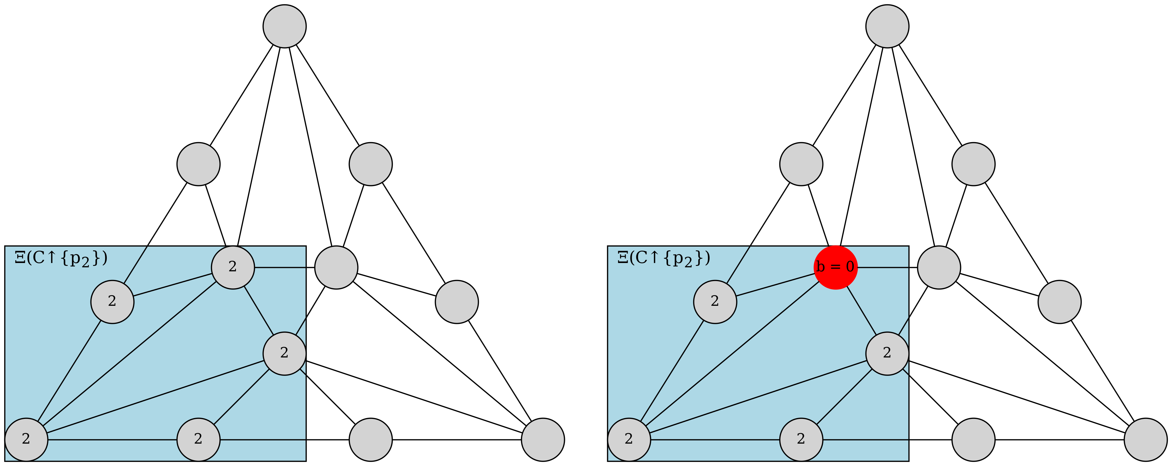
Figure 1. The 3-processes consensus task

The 3-processes consensus task

First, we will discuss the most basic requirement for the restricted protocols. A $k$-simplex $\sigma$ in $Ch(\mathcal{I})$ is called an intersection simplex of $Input(U,V)$ and $Input(U^{{}^{\prime}},V^{{}^{\prime}})$ if it is in both $Input(U,V)$ and $Input(U^{{}^{\prime}},V^{{}^{\prime}})$. Let $\sigma_{e}$ be the configuration reached from $\sigma$ by an execution in which the processes in $\sigma$ writeread each IS object simultaneously until each process in $\sigma$ outputs a value. We define an intersection $k$-simplex $\sigma$ to be compatible if the output values of the processes in $\sigma_{e}$ are the same in all protocols. We can prove that the restricted protocols must satisfy the requirement that all intersection simplices are compatible in the standard chromatic subdivision of each initial configuration. Therefore, this is a necessary condition for finalization after phase 1.

Let $\sigma$ be some intersection $k$-simplex in the standard chromatic subdivision of $C$, where $C$ is an initial configuration. In phase 1, the prover can submit a chain of queries corresponding to the schedule where the intersection simplex $\sigma$ is first reached, and then all processes in $\sigma$ are scheduled until each process outputs a value. Since the choice of $\sigma$ is finite, there are only finite numbers of chains of queries. The prover can end phase 1 by choosing any process set as the schedule, which means that any protocol for $\Xi(C\uparrow U)$ has to adopt the existing output values for the constructed configurations. This is why the adversary for the consensus task cannot finalize after phase 1 as what the adversary for the $(n,2)$-set agreement task can do: there exists a protocol for each $Input(U,V)$, but some intersection simplices cannot be compatible.

We shall now prove that this requirement is sufficient for an adversary to finalize after phase 1, which is one of the main results in this paper: the adversary can win against any restricted extension-based prover after phase 1 if there is a restricted protocol for each $Input(U,V)$ and all intersection simplices in the standard chromatic subdivision of all initial configurations are compatible. Like in previous works (AAE⁺, 19; BE, 21), we will design an adversary that can win against any extension-based prover. The adversary maintains a partial specification $\delta$ of a protocol and some invariants. All these previous sets of invariants are closely related to specific tasks, such as the $(n,k)$-set agreement task. Invariant (3) in (AAE⁺, 19) guarantees that two vertices in $S^{t}$ that terminate with different output values are sufficiently far apart, which is pointless for a general task. Therefore, these invariants must be revised. Before giving them directly, we have to discuss some preparations for our adversarial strategy.

5.2.1. Preparations

By assumption, the conditions of Theorem 5.3 are satisfied. If a task is solvable in the NIIS model, then it is solvable in the IIS model. We may assume, without loss of generality, that protocol $Protocol(U,V)$ is an IIS protocol that will terminate after some round $t(U,V)$. We can choose the largest round of termination $r_{max}$ and set all IIS protocols to end in round $r_{max}$ by having all processes defer their termination to round $r_{max}$ and output the same values as the original protocols. Now we define some core concepts in our adversarial strategy. The $n$-simplices in a chromatic subdivision of $(\mathcal{I}$ are of special importance in our discussions, and we will sometimes call them n-cliques or cliques to emphasize that their dimensions are $n$.

First, we define the protocol configuration of an n-clique. For each n-clique $s^{n}$ in $Ch^{r_{max}}(\mathcal{I})$, we can define a unique tuple $(U,V)$ for $s^{n}$, where $s^{n}$ is reached from some simplex in $Input(U,V)$. The protocol configuration of $s^{n}$ is defined as the output vector of $s^{n}$ given by $Protocol(U,V)$.

Let $s^{k}$ be a $k$-simplex in $Ch^{r_{max}}(\mathcal{I})$. The possible configurations of $s^{k}$ are defined as the restrictions to processes in $s^{k}$ of the protocol configurations of those n-cliques containing $s^{k}$. If two n-cliques have the same tuple, then the restrictions of their protocol configurations to processes in $s^{k}$ will be the same. So each possible configuration of $s^{k}$ is labeled with a tuple $(U,V)$. Note that there is at least one possible configuration for each $k$-simplex. If a $k$-simplex is in the interior of some $Input(U,V)$, then it has only one possible configuration. But for a $k$-simplex at the intersection of different $Input(U,V)$, it has multiple possible configurations. This is because an intersection simplex may terminate with the output values of different protocols in our adversarial strategy.

Let $s^{k}$ be a $k$-simplex in a subdivision of $Ch^{r_{max}}(\mathcal{I})$. The possible configurations of $s^{k}$ are defined as the restrictions to processes in $s^{k}$ of the possible configurations of $carrier(s^{k},Ch^{r_{max}}(\mathcal{I}))$. Note that if $s^{k}$ is terminated with one of its possible configurations, then there will be no violation of the task specification, since each output configuration is obtained from some valid protocol. Our definition of possible configurations can introduce some properties. For example, if each vertex of a simplex has some possible configuration with label $(U,V)$, then this simplex will also have a possible configuration with label $(U,V)$.

We must assume that $r_{max}\geq 2$ for the next definition. This assumption is without loss of generality since, if $r_{max}=1$, the termination of each protocol can be postponed by one round, as stated above. If an n-clique $s^{n}$ in $Ch^{r_{max}-1}(Input(U,V))$ has an intersection with another $Input(U^{{}^{\prime}},V^{{}^{\prime}})$ for some label $(U^{{}^{\prime}},V^{{}^{\prime}})$, the vertices of $s^{n}$ can be sorted into two types: intersection vertices and internal vertices. The intersection vertices are those vertices located at the intersection of two subcomplexes. In other words, the intersection vertices have possible configurations with $(U,V)$ and $(U^{{}^{\prime}},V^{{}^{\prime}})$. The internal vertices are in one subcomplex and have only one possible configuration with the label $(U,V)$ or $(U^{{}^{\prime}},V^{{}^{\prime}})$.

Let $C$ be an input configuration which is represented by an $n$-simplex $\sigma$. We restrict our view to the chromatic subdivision of $\sigma$. For an n-clique $s^{n}_{1}$ with label $(U,V)$ in $Ch^{r_{max}}(\sigma)$, if $s^{n}_{1}$ has an intersection with $Input(U^{{}^{\prime}},V^{{}^{\prime}})$, we define an opposite clique of $s^{n}_{1}$ with label $(U^{{}^{\prime}},V^{{}^{\prime}})$ as an n-clique $s^{n}_{2}$ in $Ch^{r_{max}}(\sigma)$ such that

• $s^{n}_{2}$ is in $Ch^{r_{max}-1}(Input(U^{{}^{\prime}},V^{{}^{\prime}}))$.

• For each intersection vertex $v$ of $s^{n}_{1}$ and $ids(v)=p$, the vertex $v$ is in $s^{n}_{2}$.

• For each internal vertex $v$ of $s^{n}_{1}$ and $ids(v)=p$, there exists an internal vertex $v^{{}^{\prime}}$ of $s^{n}_{2}$ with the process id $p$ such that $carrier(v,\sigma)=carrier(v^{{}^{\prime}},\sigma)$.

Lemma 5.4.

Let $s^{k}$ be a $k$-simplex in a subdivision of $\sigma$. A subsimplex $\tau$ of $\sigma$ is $carrier(s^{k},\sigma)$ if and only if $\tau$ is the union of $\{carrier(v,\sigma)\allowbreak|v\in s^{k}\}$.

Proof.

Let $\tau^{{}^{\prime}}$ be the subsimplex of $\sigma$ whose vertices set $V$ is the union of a collection of vertices sets, each of which is the vertices set of $carrier(v,\sigma)$ for some $v\in s^{k}$. Each point $x$ in $s^{k}$ can be expressed as a combination of vertices of $s^{k}$, that is, $x=\sum_{i=0}^{k}t_{i}v_{i}$ where $\sum_{i=0}^{k}t_{i}=1$ and $t_{i}\geq 0$ for all i. At the same time, each vertex $v_{i}$ of $s^{k}$ can be expressed as a combination of vertices of $carrier(v_{i},\sigma)$, i.e. $v_{i}=\sum_{i=0}^{k^{{}^{\prime}}}t^{{}^{\prime}}_{i}v^{{}^{\prime}}_{i}$ where $\sum_{i=0}^{k^{{}^{\prime}}}t^{{}^{\prime}}_{i}=1$, $v^{{}^{\prime}}_{i}$ is in $V$ and $t^{{}^{\prime}}_{i}>0$ for all i. Each point $x$ in $s^{k}$ can be expressed as a combination of vertices of $V$, and the coefficients are all positive when expressing the barycenter of $s^{k}$. So $\tau^{{}^{\prime}}$ is the carrier of $s^{k}$ in $\sigma$ and any subsimplex of $\tau^{{}^{\prime}}$ is not the carrier of $s^{k}$. ∎

By the definition of opposite cliques, each subsimplex of an n-clique will have the same carrier as the corresponding subsimplex of its opposite clique, and we have the following lemma.

Lemma 5.5.

For an n-clique $s^{k}$ with label $(U,V)$ in $Ch^{r_{max}}(C)$, the output configuration of an opposite clique with label $(U^{{}^{\prime}},V^{{}^{\prime}})$ when using $Protocol(U^{{}^{\prime}},V^{{}^{\prime}})$ is a valid output configuration for $s^{k}$ that will not violate the carrier map.

We now show that an n-clique having an intersection with subcomplex $Ch^{r_{max}-1}(Input(U,V))$ will have an opposite clique with label $(U,V)$. Let $C$ be an input configuration represented by a simplex $\sigma$. Each simplex in $Ch^{r}(\sigma)$ represents a configuration reached from $C$ by a $r$-round schedule. Each round is a partition of the set of all processes, denoted $\Pi$. A vertex in $Ch^{r}(\sigma)$ is uniquely determined by the set of processes that it reads in each partition of $\Pi$. So, if some process $p$ reads the same set of processes in two configurations in $Ch(\sigma)$, then the vertex with process id $p$ is shared by two configurations. We will use this result in later proofs.

A proposition is needed to prove the third requirement of opposite cliques.

Proposition 5.6.

Suppose that some n-clique $s^{n}_{1}$ in $Ch(\sigma)$ has an intersection with $Input(U,V)$. Let $P$ denote the set of ids of the intersection vertices. If some $n$-simplex $s^{n}_{2}$ in $Ch(s^{n}_{1})$ has an intersection with $Ch(Input(U,V))$, the second partition of $\Pi$ in the schedule from $\sigma$ to $s^{n}_{2}$ will start with a process set that contains some process in $P$.

Lemma 5.7.

For an n-clique $s^{n}$ in $Ch^{r_{max}}(\sigma)$ having an intersection with $Ch^{r_{max}-1}(Input(U,V))$, there exists an opposite clique of $s^{n}$ with label $(U,V)$ if $r_{max}\geq 2$.

Proof.

For two process set $U_{1}$ and $U_{2}$ such that $|U_{1}|\leq|U_{2}|$, Lemma 10.4.4 in (HKR, 13) states that the intersection $\Xi(C\uparrow U_{1})\bigcap\allowbreak\Xi(C\uparrow U_{2})$ equals $(\Xi\downarrow W)(C\uparrow U_{1}\bigcup U_{2})$ where $W=U_{1}$ if $U_{1}\subseteq U_{2}$ , otherwise $W=U_{1}\bigcup U_{2}$. We will discuss the two cases respectively.

We will first prove the case that $U_{1}\nsubseteq U_{2}$. Consider the standard chromatic subdivision $Ch^{1}(\sigma)$. For any two process set $U_{1}$ and $U_{2}$ that satisfy $|U_{1}|\leq|U_{2}|$ and $U_{1}\nsubseteq U_{2}$, the intersection $\Xi(C\uparrow U_{1})\bigcap\Xi(C\uparrow U_{2})$ will be $(\Xi\downarrow U_{1}\bigcup U_{2})(C\uparrow U_{1}\bigcup U_{2})$. The intersection contains all the configurations reached by some $(\Pi-U_{1}\bigcup U_{2})$-only schedule when the input values of $U_{1}\bigcup U_{2}$ have been read by all processes in $(\Pi-U_{1}\bigcup U_{2})$. In other words, it is a simplicial complex consisting of $(|\Pi|-|U_{1}\bigcup U_{2}|)$-simplices and their subsimplices, and each $(|\Pi|-|U_{1}\bigcup U_{2}|)$-simplex corresponds to an ordered partition of processes in $(\Pi-U_{1}\bigcup U_{2})$.

In $\Xi(C\uparrow U_{1})$, each n-simplex corresponds to an ordered partition of the processes in $(\Pi-U_{1})$. If an n-simplex $C_{1}$ in $\Xi(C\uparrow U_{1})$ contains a $(|\Pi|-|U_{1}\bigcup U_{2}|)$-simplex at the intersection, then its schedule can be expressed as a concatenation of $U_{1}$, an ordered partition of $U_{2}-U_{1}$ and an ordered partition of $(\Pi-U_{1}\bigcup U_{2})$, or a special case where the last process set of the former partition is merged with the first process set of the latter partition. We can choose the n-simplex $C_{2}$ reached from $C$ by the schedule generated by concatenating $U_{2}$, $U_{1}$ and the same ordered partition of $(\Pi-U_{1}\bigcup U_{2})$. For any n-simplex $C_{3}$ reached from $C_{1}$ by a schedule $\gamma$ and having an intersection with $Input(U_{2},V_{2})$, we choose the n-simplex $C_{4}$ reached from $C_{2}$ by the same schedule $\gamma$ as its opposite clique. Therefore, the n-simplex $C_{4}$ is in $\Xi(C\uparrow U_{2})$, and the first requirement of the opposite clique is satisfied. The carrier of each vertex of a configuration reached from $C$ depends only on the set of processes it has seen(directly or indirectly). The schedules from $C$ to $C_{3}$ and to $C_{4}$ only differ in the first partition of $\Pi$, and only the processes in ${U_{1}\bigcup U_{2}}$ will see the input values of a different subset of ${U_{1}\bigcup U_{2}}$. The opposite vertices of intersection vertices whose ids are in $\Pi-U_{1}\bigcup U_{2}$ are therefore the vertices themselves. The second requirement of the opposite clique is satisfied. The intersection vertices of $C_{3}$ and $C_{4}$ have the same carrier. However, it is possible that the vertices in $C_{3}$ and $C_{4}$ with ids in ${U_{1}\bigcup U_{2}}$ have different carriers. This is exactly what happens with the configurations $C_{1}$ and $C_{2}$. But the mismatch will disappear after one more subdivision. In $Ch^{2}(\sigma)$, if an n-simplex $C_{3}$ reached from $C_{1}$ has an intersection with $Input(U_{2},V_{2})$, then the second partition of $\Pi$ in the schedule from $C$ to $C_{3}$ must begin with a process set containing some process in $(\Pi-U_{1}\bigcup U_{2})$ that has already seen input values of ${U_{1}\bigcup U_{2}}$. Each process in $C_{3}$ will know the input values of ${U_{1}\bigcup U_{2}}$. Therefore, the carrier of each vertex in $C_{3}$ will be the same as the carrier of the corresponding vertex in $C_{4}$ as it sees the same set of input values. The third requirement of the opposite clique is satisfied. Now we have shown that $C_{4}$ is the opposite clique of $C_{3}$.

But in $Ch^{1}(\sigma)$, the n-cliques in $\Xi(C\uparrow U_{1})$ having an intersection with $\Xi(C\uparrow U_{2})$ are not limited to the n-simplices we have discussed. There could be an n-simplex $C_{1}$ that contains only a subsimplex of those $(|\Pi|-|U_{1}\bigcup U_{2}|)$-simplices at the intersection. Its schedule can be expressed as a concatenation of $U_{1}$, an ordered partition of $(U_{2}-U_{1})\bigcup D$ and an ordered partition of $(\Pi-U_{1}\bigcup U_{2}-D)$ for some subset $D$ of $(\Pi-U_{1}\bigcup U_{2})$. Consider the last process set $U_{l}$ of the ordered partition of $(U_{2}-U_{1})\bigcup D$. It must contain some process in $(U_{2}-U_{1})$, and let $D_{l}$ be those processes in $U_{l}$ that are also in $D$. The vertices with ids in $(\Pi-U_{1}\bigcup U_{2}-D)\bigcup D_{l}$ are the intersection vertices. The limitation of an ordered partition of a set $U$ to a subset $U^{{}^{\prime}}\subset U$ is defined as an ordered partition of $U^{{}^{\prime}}$ generated by removing all processes not in $U^{{}^{\prime}}$ from the original ordered partition. We can choose the n-simplex $C_{2}$ reached from $C$ by the schedule generated by concatenating $U_{2}$, $U_{1}-U_{2}$, the limitation of the same ordered partition of $(U_{2}-U_{1})\bigcup D$ to the process set $D$ and the same ordered partition of $(\Pi-U_{1}\bigcup U_{2}-D)$. As in the previous case, for any n-simplex $C_{3}$ reached from $C_{1}$ by a schedule $\gamma$ that has an intersection with $Input(U_{2},V_{2})$, we choose the n-simplex $C_{4}$ reached from $C_{2}$ by the same schedule $\gamma$ as its opposite clique. The first requirement of the opposite clique is satisfied. Only processes in $U_{1}\bigcup U_{2}\bigcup D-D_{l}$ can see the input values of a different subset of $U_{1}\bigcup U_{2}\bigcup D$ after changing the first partition of $\Pi$. The intersection vertices are those in $(\Pi-U_{1}\bigcup U_{2}-D+D_{l})$, and the opposite vertices of the intersection vertices are therefore the vertices themselves. The second requirement of the opposite clique is satisfied. In $Ch^{2}(\sigma)$, if an n-simplex $C_{3}$ reached from some $C_{1}$ has an intersection with $Input(U_{2},V_{2})$, then the second partition of $\Pi$ in the schedule from $C$ to $C_{3}$ must begin with a process set that contains some process in $(\Pi-U_{1}\bigcup U_{2}-D+D_{l})$ that has already seen the input values of $U_{1}\bigcup U_{2}\bigcup D$. Processes whose ids are in ${U_{1}\bigcup U_{2}\bigcup D}$ will know the input values of ${U_{1}\bigcup U_{2}\bigcup D}$. Therefore, the third requirement of the opposite clique is satisfied and $C_{4}$ is the opposite clique of $C_{3}$. We have discussed all n-simplices in $\Xi(C\uparrow U_{1})$ having an intersection with $\Xi(C\uparrow U_{2})$ and found an opposite clique for each of them. In fact, the simplices discussed in the last paragraph belong to a special case where $D$ is an empty set. By symmetry, we can also find an opposite clique for all n-simplices in $\Xi(C\uparrow U_{2})$ having an intersection with $\Xi(C\uparrow U_{1})$.

Then we will prove the case that $U_{1}\subseteq U_{2}$. The proof techniques are almost identical as in the former case. The intersection $\Xi(C\uparrow U_{1})\bigcap\Xi(C\uparrow U_{2})$ will be $(\Xi\downarrow U_{1})(C\uparrow U_{2})$. In $Ch^{1}(\sigma)$, the schedule of an n-simplex $C_{1}$ in $\Xi(C\uparrow U_{1})$ having some vertices at the intersection can be expressed as a concatenation of $U_{1}$, an ordered partition of $(U_{2}-U_{1})\bigcup D$ and an ordered partition of $(\Pi-U_{2}-D)$ for some subset $D$ of $(\Pi-U_{2})$. We can choose the n-simplex $C_{2}$ reached by the schedule generated by concatenating $U_{2}$, the limitation of the same ordered partition of $(U_{2}-U_{1})\bigcup D$ to $D$ and the same ordered partition of $(\Pi-U_{2}-D)$. For any n-simplex $C_{3}$ reached from $C_{1}$ by a schedule $\gamma$, the n-simplex $C_{4}$ reached from $C_{2}$ by the same schedule $\gamma$ is chosen as its opposite clique. Three requirements of an opposite clique can be checked, as in the former case. If an n-simplex in $\Xi(C\uparrow U_{2})$ has an intersection with $Input(U_{1},V_{1})$, we simply choose it as its opposite clique, since the protocol for $\Xi(C\uparrow U_{1})$ can be applied to $Input(U_{2},V_{2})$. ∎

According to Lemma 5.7, for an n-clique $\sigma$ in $Ch^{r_{max}}(\mathcal{I})$ that has an intersection with $Input(U,V)$ , there exists an opposite clique of $\sigma$ with the label $(U,V)$ if $r_{max}\geq 2$. If we have to terminate some vertices with the label $(U,V)$ in a subdivision of $\sigma$, we can always find an opposite clique and use its protocol configuration as the terminated values without violating the task specification. But an important question remains to be answered: are these terminated values well-defined? In other words, if two n-cliques share some vertex $v$ with process id $p$, then will their opposite cliques with the label $(U,V)$ share the output value of $p$ when using $Protocol(U,V)$? The following lemmas tell us that terminated values are well-defined.

Lemma 5.8.

If two n-cliques in $Ch^{r_{max}}(\sigma)$ both have opposite cliques with label $(U,V)$ and share some vertex $v$ with process id $p$, then the two vertices in their opposite cliques that have process id $p$ will have the same output value when using protocol $Protocol(U,V)$.

Proof.

Suppose that the two n-cliques $C_{3}$ and $C_{3}^{{}^{\prime}}$ are reached from $C_{1}$ and $C_{1}^{{}^{\prime}}$ in $Ch^{1}(\sigma)$ by the schedules $\gamma_{1}$ and $\gamma_{2}$, respectively. Note that n-cliques $C_{1}$ and $C_{1}^{{}^{\prime}}$ may not be in the same subcomplex $Input(U,V)$. We will use the notation in the previous proof to simplify the understanding. Because the vertex $v$ is shared by $C_{3}$ and $C_{3}^{{}^{\prime}}$, the process $p$ will see the same set of processes in each partition of $\Pi$.

If $C_{1}$ and $C_{1}^{{}^{\prime}}$ are the same n-clique, then using the strategy in the proof of Lemma 5.7, the opposite cliques of $C_{3}$ and $C_{3}^{{}^{\prime}}$ are reached from the same n-clique in $Ch^{1}(\sigma)$ by the schedules $\gamma_{1}$ and $\gamma_{2}$, respectively. Since the vertex $v$ is shared by $C_{3}$ and $C_{3}^{{}^{\prime}}$, their opposite cliques will also share the vertex having process id $p$ in our construction. The output values are given by the same protocol and are therefore identical.

Suppose that $C_{1}$ and $C_{1}^{{}^{\prime}}$ are not the same clique but still in the same subcomplex $\Xi(C\uparrow U)$. Considering the case where $U_{1}\nsubseteq U_{2}$, by symmetry, we can simply assume that $C_{1}$ and $C_{2}$ are in $\Xi(C\uparrow U_{1})$. The schedule from $C$ to $C_{1}$ can be expressed as a concatenation of $U_{1}$, an ordered partition of $(U_{2}-U_{1})\bigcup D_{1}$ and an ordered partition of $(\Pi-U_{1}\bigcup U_{2}-D_{1})$, for some subset $D_{1}$ of $(\Pi-U_{1}\bigcup U_{2})$. The schedule from $C$ to $C_{1}^{{}^{\prime}}$ can also be presented for some subset $D_{2}$. The n-clique $C_{2}$ is defined as the n-simplex reached from $C$ by the schedule generated by concatenating $U_{2}$, $U_{1}$, the limitation of the same ordered partition of $(U_{2}-U_{1})\bigcup D_{1}$ to process set $D_{1}$ and the same ordered partition of $(\Pi-U_{1}\bigcup U_{2}-D_{1})$. And $C_{2}^{{}^{\prime}}$ is defined in the same way. We will show that the opposite cliques reached from $C_{2}$ and $C_{2}^{{}^{\prime}}$ share the vertex with the process id $p$.

We need to analyze the first partition of $\Pi$. Suppose that the vertex with process id $p$ is shared by $C_{1}$ and $C_{1}^{{}^{\prime}}$. There are four possible cases depending on where the process $p$ is.

• If $p\in U_{2}$, then the process $p$ will see the input values of the processes in $U_{2}$ in both $C_{2}$ and $C_{2}^{{}^{\prime}}$.

• If $p\in U_{1}-U_{2}$, then the process $p$ will see the input values of the processes in $U_{1}\bigcup U_{2}$ in both $C_{2}$ and $C_{2}^{{}^{\prime}}$.

• If $p\in D_{1}\bigcup D_{2}$, the vertex $v$ in $C_{1}$ and $C_{1}^{{}^{\prime}}$ will see the same subset of $\Pi-U_{1}\bigcup U_{2}$, and the same subset of $U_{1}\bigcup U_{2}$ since it is a shared vertex of $C_{1}$ and $C_{1}^{{}^{\prime}}$ by assumption. By construction, the process $p$ will see $U_{1}\bigcup U_{2}$(not a subset of it) and the same subset of $D_{1}\bigcup D_{2}$ in $C_{2}$ and $C_{2}^{{}^{\prime}}$.

• If $p\in\Pi-U_{1}\bigcup U_{2}-D_{1}\bigcup D_{2}$, then the adjustment of the first partition will not affect the set of processes it sees.

In each case, the sets of processes that $p$ will see in $C_{2}$ and $C_{2}^{{}^{\prime}}$ are the same. So if any vertex is shared by $C_{1}$ and $C_{1}^{{}^{\prime}}$, $C_{2}$ and $C_{2}^{{}^{\prime}}$ will share the vertex with the same process id. Recall that the schedules $\gamma_{1}$ from $C_{1}$ to $C_{3}$ and $\gamma_{2}$ from $C_{1}^{{}^{\prime}}$ to $C_{3}^{{}^{\prime}}$ are indistinguishable to the process $p$. The opposite cliques of $C_{3}$ and $C_{3}^{{}^{\prime}}$ are reached from $C_{2}$ and $C_{2}^{{}^{\prime}}$ by $\gamma_{1}$ and $\gamma_{2}$, respectively. So, the opposite cliques of $C_{3}$ and $C_{3}^{{}^{\prime}}$ share the vertex with the process id $p$.

Now consider the case $U_{1}\subseteq U_{2}$. If $C_{1}$ and $C_{1}^{{}^{\prime}}$ are $\Xi(C\uparrow U_{2})$, the chosen n-clique $C_{2}$ and $C_{2}^{{}^{\prime}}$ are $C_{1}$ and $C_{1}^{{}^{\prime}}$. Therefore, a common vertex $v$ is also a common vertex of their opposite cliques. If $C_{1}$ and $C_{1}^{{}^{\prime}}$ are in $\Xi(C\uparrow U_{1})$. The schedule from $C$ to $C_{1}$ can be expressed as a concatenation of $U_{1}$, an ordered partition of $(U_{2}-U_{1})\bigcup D_{1}$ and an ordered partition of $(\Pi-U_{2}-D_{1})$, for some subset $D_{1}$ of $(\Pi-U_{2})$. We can use almost the same proof techniques here as in the previous paragraph. We can discuss different cases of adjustment of the first partition and prove that opposite cliques of $C_{3}$ and $C_{3}^{{}^{\prime}}$ will share the vertex with the process id $p$. A detailed proof is omitted to avoid redundancy. In fact, the proof here can be included in the proof structure presented in the previous paragraph as a special case that $U_{1}\subseteq U_{2}$ or $U_{2}\subseteq U_{1}$. This observation can simplify the remaining proof.

Suppose that $C_{1}$ and $C_{1}^{{}^{\prime}}$ are not in the same subcomplex $\Xi(C\uparrow U)$. We will denote their first process sets by $U_{1}$ and $U_{1}^{{}^{\prime}}$. Then the schedule from $C$ to $C_{1}$ is expressed as above, and the schedule from $C$ to $C_{1}^{{}^{\prime}}$ can be expressed as a concatenation of $U_{1}^{{}^{\prime}}$, an ordered partition of $(U_{2}-U_{1}^{{}^{\prime}})\bigcup D_{2}$ and an ordered partition of $(\Pi-U_{1}^{{}^{\prime}}\bigcup U_{2}-D_{2})$, for some subset $D_{2}$ of $(\Pi-U_{1}^{{}^{\prime}}\bigcup U_{2})$. If the vertex $v$ with the process id $p$ is shared by $C_{1}$ and $C_{1}^{{}^{\prime}}$, then the process $p$ is in $\Pi-U_{1}\bigcap U_{1}^{{}^{\prime}}$, and has seen the input values of $U_{1}\bigcup U_{1}^{{}^{\prime}}$ in $C_{1}$ and $C_{1}^{{}^{\prime}}$. The process $p$ sees the same set of processes in $C_{1}$ and $C_{1}^{{}^{\prime}}$, and we will argue that it sees the same set of processes in $C_{2}$ and $C_{2}^{{}^{\prime}}$.

Consider the set of processes that $p$ will see in $C_{2}$:

• If $p\in U_{2}$, then the process $p$ will see the input values of $U_{2}$ in $C_{2}$ and $C_{2}^{{}^{\prime}}$.

• If $p\in U_{1}-U_{2}$, it sees the input values of $U_{1}$ in $C_{1}$ and sees the input values of $U_{1}\bigcup U_{2}$ in $C_{2}$. The new processes that $p$ sees are those in $U_{2}-U_{1}$.

• If $p\in D_{1}$, the new processes that process $p$ will see are those in $U_{2}$ that it does not see in $C_{1}$.

• If $p\in\Pi-U_{1}\bigcup U_{2}-D_{1}$, no new information is obtained by the process $p$.

In case 1 where $p\in U_{2}$, $p$ will see $U_{2}$ in both $C_{2}$ and $C_{2}^{{}^{\prime}}$. In cases 2, 3 and 4 where $p\notin U_{2}$, the new processes are those in $U_{2}$ that process $p$ does not see in $C_{1}$ and $C_{1}^{{}^{\prime}}$. Therefore, the process $p$ will see the same set of processes in $C_{2}$ and $C_{2}^{{}^{\prime}}$. If any vertex is shared by $C_{1}$ and $C_{1}^{{}^{\prime}}$, $C_{2}$ and $C_{2}^{{}^{\prime}}$ will share the vertex with the same process id. The opposite cliques of $C_{3}$ and $C_{3}^{{}^{\prime}}$ reached from $C_{2}$ and $C_{2}^{{}^{\prime}}$ will share the vertex with the process id $p$.

∎

Finally, we need to consider the case that two n-cliques in $Ch^{r_{max}}(I)$ are not reached from a single initial configuration $C$.

Lemma 5.9.

If two n-cliques in $Ch^{r_{max}}(\sigma_{1})$ and $Ch^{r_{max}}(\sigma_{2})$ both have an opposite clique with label $(U,V)$ and share some vertex $v$ with the process id $p$, then the two vertices in their opposite cliques having the process id $p$ will have the same output value when using protocol $Protocol(U,V)$.

Proof.

Let $s_{b}$ be the largest common simplex of $\sigma_{1}$ and $\sigma_{2}$. The vertex $v$ is in $Ch^{r_{max}}(s_{b})$. So $carrier(v,\sigma_{1})$ and $carrier(v,\sigma_{2})$ are the same simplex $s_{c}$, which is a subsimplex of $s_{b}$. Therefore, the two vertices with the process id $p$ of two opposite cliques are both in $Ch^{r_{max}}(s_{c})$. By the symmetry of construction, we know that the two vertices are the same and have the same output value when using the restricted protocol $Protocol(U,V)$. ∎

Active distance is an essential tool in our adversarial strategy. The active distance between subgraphs $A$ and $B$ of a graph $G$ is defined to be the minimal number of edges between non-terminated vertices in any path from $A$ to $B$ in $G$. An important property is that the active distance between $\chi(A)$ and $\chi(B)$ in the non-uniform chromatic subdivision of $G$ is double the active distance between $A$ and $B$ in $G$. This property allows the adversary to subdivide a graph finitely to make certain subgraphs distant enough from each other.

5.2.2. Adversarial strategy in phase 1

We define an adversarial strategy so that, before and after each query made by the prover in phase 1, the adversary is able to maintain some invariants. The adversary maintains a partial specification of $\Delta$ (the protocol it is adaptively constructing) and an integer $t\leq 0$. The integer $t$ represents the number of non-uniform chromatic subdivisions of the input complex, $S^{0}$, that it has performed. The specification of $\Delta$ is defined using a sequence of graphs indexed by an integer $t$, and each graph $S^{t}$ represents all configurations reachable from the initial configurations by a $t$-round schedule. When the prover submits a query in the first phase, the adversary may increment $t$ and set $\Delta$ values for some vertices so that it can respond to the prover while maintaining the invariants. Note that our invariant (1) is the same as the invariant (1) in (AAE⁺, 19), and our adversarial strategy is inspired by theirs. The invariants will use the concepts defined in Section 5.2.1.

• For each $0\leq r<t$ and each vertex $v\in S^{r}$ , $\Delta(v)$ is defined. If $v$ is a vertex in $S^{t}$, then either $\Delta(v)$ is undefined or $\Delta(v)\neq\perp$. If $s$ is the state of a process in a configuration that has been reached by the prover, then $s$ is a vertex in $S^{r}$, for some $0\leq r\leq t$, and $\Delta(s)$ is defined.

• Let $s^{k}$ be a $k$-simplex representing a terminated configuration in $S^{t}$. Then $s^{k}$ is in the subdivision of some n-clique of $Ch^{r_{max}}(\mathcal{I})$ and has a tuple $(U,V)$ as its label. There exists a $k^{{}^{\prime}}$-simplex $s^{k^{{}^{\prime}}}$ that is terminated with some possible configuration of it(including the output values and the label) such that there is a path consisting of terminated vertices from $s^{k}$ to $s^{k^{{}^{\prime}}}$.

• Let $s^{k_{1}}$ and $s^{k_{2}}$ be two terminated simplices with different labels in $S^{t}$. The active distance between $s^{k_{1}}$ and $s^{k_{2}}$ in $S^{t}$ is at least 3.

Initially, the adversary sets $\Delta(v)=\perp$ for each vertex $v\in S^{0}$. Then it subdivides $S^{0}$ to construct $S^{1}$ and set $t=1$. To keep the invariant (2) true, repeat this subdivision $r_{max}+r_{add}$ times and set $t=r_{max}+r_{add}+1$, for some constant number $r_{add}\geq 1$. All vertices in $S^{r}$ where $r\leq r_{max}+r_{add}$ will be defined with the value $\perp$, and all vertices in $S^{r_{max}+r_{add}+1}$ will be undefined. Before the first query, the prover has only reached the initial configurations and there is no terminated configuration. Therefore, the invariants are satisfied at the beginning of phase 1.

Now suppose that the invariants are satisfied immediately prior to a query $(C,P)$ by the prover, where $C$ is a configuration previously reached by the prover and $P$ is a set of active processes in $C$ poised to access the same snapshot object. There is an integer $0\leq r\leq t$ such that the states of the processes in $P$ correspond to a simplex in $S^{r}$ by the first invariant. Since the processes in $P$ are still active in $C$, $\Delta(v)=\perp$ for each such vertex $v$ and $r<t$. Let $\sigma$ be the simplex in $S^{r+1}$ whose vertices represent the states of processes in $P$ in the resulting configuration.

If $0\leq r<t-1$, then $\Delta$ is already defined for $\sigma$ in $S^{r+1}$ according to the invariant (1). The adversary does nothing and returns the defined values of $\Delta$. Since $\Delta$ has not changed, the invariants continue to hold.

If $r=t-1$, then $\sigma$ in $S^{t}$ may contain some undefined vertices. The adversary has to define the $\Delta$ values for these undefined vertices. For each undefined vertex $v$ having a process id $p$ in $\sigma$, there are three assignment rules:

• If there is a possible label $(U,V)$ for the vertex $v$ such that the active distance between $v$ and any terminated configuration with a different label is at least 3, the adversary will set $\Delta(v)$ as the output value of its possible configuration with label $(U,V)$.

• If there is some vertex in $\sigma$ that is already terminated with the label $(U^{{}^{\prime}},V^{{}^{\prime}})$, and the active distance between $v$ and any terminated configuration with a label different from $(U^{{}^{\prime}},V^{{}^{\prime}})$ is at least 3, the adversary can terminate the vertex $v$ with the label $(U^{{}^{\prime}},V^{{}^{\prime}})$ although $(U^{{}^{\prime}},V^{{}^{\prime}})$ is not the label of a possible configuration of $v$. Let $\sigma^{{}^{\prime}}$ be the opposite clique with label $(U^{{}^{\prime}},V^{{}^{\prime}})$ of the n-clique containing vertex $v$. The value of $\Delta$ for $v$ is the output value of the process $p$ in $\sigma^{{}^{\prime}}$ using $Protocol(U^{{}^{\prime}},V^{{}^{\prime}})$. We declare that if the vertex $v$ is contained in different n-cliques, then the choice of n-cliques will not change the terminated value of $v$. The proof of this assertion will be given in Section 5.2.3.

• Otherwise, the adversary will set $\Delta(v)=\perp$.

We introduce rule (2) to avoid an infinite chain of queries. However, this rule cannot be used frequently, since only those n-cliques that have an intersection with $Ch^{r_{max}-1}(Input(U,V))$ will have an opposite clique with the label $(U,V)$. We impose a restriction on this rule: If rule (2) is applied to a vertex in $S^{n_{1}}$, then it can only be used again in $S^{n_{2}}$ if $n_{2}-n_{1}>=r_{spe}$ for some constant number $r_{spe}$.

If the adversary sets $\Delta(v)\neq\perp$ for each vertex $v\in\sigma$, the invariant (1) holds. Otherwise, some vertex terminates with the value $\perp$, and the requirement for $S^{t}$ is not satisfied. The adversary will define $\Delta(v)=\perp$ for each vertex $v\in S^{t}$ where $\Delta(v)$ is undefined, subdivide $S^{t}$ to create $S^{t+1}$ and increment $t$. Invariant (1) continues to hold after the subdivision.

If two vertices are connected by a terminated path, they will have the same active distance to any other terminated configuration. Invariant (3) holds since newly terminated vertices will be checked in rules (1) and (2), and a subdivision doubles the active distances between terminated configurations with different labels. Invariant (2) is more complicated to analyze. It is affected only when $r=t-1$ and some undefined vertices in $S^{t}$ are terminated, that is, given some values other than $\perp$. By the induction hypothesis, we only have to discuss the simplex $\sigma_{n}$ consisting of all newly terminated vertices. If all vertices are terminated by rule (1), then each vertex in $\sigma_{n}$ is terminated with its possible configuration with some label $l_{nt}$. By the property of possible configurations, we know that $\sigma_{n}$ is terminated with its possible configurations with the label $l_{nt}$. Invariant (2) still holds. Otherwise, some vertex of $\sigma_{n}$ is terminated by rule (2) with the label $l_{nt}$. By construction, we know that there is some adjacent configuration $\sigma_{adj}$ that is terminated with the label $l_{nt}$ before this query. Using the induction hypothesis, there exists an $k^{{}^{\prime}}$-simplex $s^{k^{{}^{\prime}}}$ terminated with some possible configuration such that there is a path consisting of terminated vertices from $\sigma_{adj}$ to $s^{k^{{}^{\prime}}}$. There is also a path consisting of terminated vertices from $\sigma_{n}$ to $s^{k^{{}^{\prime}}}$. The invariant (2) continues to hold.

Therefore, the adversary can maintain all invariants after the prover submits a query in the first phase.

5.2.3. The prover cannot win in the first phase

There are only two ways the prover can win. First, the prover can find a violation of the task specification, i.e. some terminated configuration should not be assigned with its output values. We have argued in previous sections that if a simplex $\sigma$ is terminated with one of its possible configurations, then it will not cause any violation of the task specification. But an innovation of our adversary strategy is that some vertices may not be terminated with their possible configurations by rule (2). Since the opposite cliques will be used in rule (2), we have to prove that there is no abuse of rule (2).

Lemma 5.10.

If a vertex $v$ is terminated by rule (2) with label $(U,V)$, then any n-clique in $Ch^{r_{max}}(\mathcal{I})$ that contains the carrier of $v$ in $Ch^{r_{max}}(\mathcal{I})$ will have an opposite clique with label $(U,V)$.

Proof.

The invariant (2) guarantees that a vertex terminated with label $(U,V)$ by rule (2) has a path consisting of terminated vertices to some vertex that is terminated with its possible configuration with label $(U,V)$. This path consists of vertices terminated by rule (2). We will argue that this path is contained in some n-cliques in $Ch^{r_{max}}(\mathcal{I})$, each of which has an opposite clique with the label $(U,V)$.

It has been shown that there exists an equivalent geometric definition of the standard chromatic subdivision in each algebraic topology textbook. Let $K$ be a geometric simplicial complex. The mesh of $K$, denoted $mesh(K)$, is the maximum diameter of any of its simplices or, equivalently, the length of its longest edge. The standard chromatic subdivision is a mesh-shrinking subdivision which means that the mesh of a simplex will decrease after such a subdivision. And in (HS, 99) it is proved that $mesh(Ch(s^{k}))\leq\frac{n}{n+1}mesh(s^{k})$ for any $k$-simplex $s^{k}$. Let $l_{m}$ denote the mesh of $Ch^{r_{max}}(C)$. Since no vertex in $Ch^{r_{max}}(C)$ has terminated, $l_{m}$ is well-defined. Note that the adversary uses the non-uniform chromatic subdivision to construct $S^{r+1}$ from $S^{r}$ for each $r\leq r_{max}+r_{add}$. The length of an edge between a terminated vertex and an adjacent vertex will not change after a non-uniform chromatic subdivision. But the length of an edge between two active vertices in $S^{r}$ where $r\geq r_{max}$ is at most $(\frac{n}{n+1})^{r-r_{max}}*l_{m}$. Consider the path $v_{0},v_{1},v_{2},\cdots v_{k}$ where $v_{0}$ terminates with one of its possible configurations. When $v_{i}$ where $i\geq 0$ is terminated in $S_{r}$, the distance between $v_{i}$ and $v_{i+1}$ will have an upper limit $(\frac{n}{n+1})^{r-r_{max}}*l_{m}$. If $v_{i+1}$ is a vertex adjacent to $v_{i}$ in $S^{r}$, the upper bound is reached. Otherwise $v_{i+1}$ is terminated in a later subdivision and the distance between $v_{i}$ and $v_{i+1}$ is less than the distance between $v_{i}$ and an adjacent vertex in $S_{r}$. Therefore, the total length of the path has a limitation $\lim\limits_{k\rightarrow\infty}\sum_{i=0}^{k}|v_{i+1}-v_{i}|\leq l_{m}*(\frac{n}{n+1})^{r_{add}}/(1-(\frac{n}{n+1})^{r_{spe}})$. Let $D$ denote the subcomplex of $Ch^{r_{max}}(\mathcal{I})$, which consists of all simplices that do not have an intersection with $Input(U,V)$. Then there is a minimum distance from $Input(U,V)$ to $D$. If we choose $r_{add}$ and $r_{spe}$ large enough, we can avoid any path consisting of vertices terminated by rule (2) to reach $D$. All vertices terminated by rule (2) are contained in the n-cliques in $Ch^{r_{max}}(\mathcal{I})$ that have an intersection with $Input(U,V)$. ∎

Recall that we assert that if a vertex $v$ terminated by rule (2) is contained in different n-cliques, then the choice of the n-clique will not change the terminated value of $v$. Lemma 5.8 and Lemma 5.9 tell us that the process $p$ will have the same value in the output configurations with the label $(U,V)$ of two n-cliques in $Ch^{r_{max}}(\mathcal{I})$ if the two n-cliques both have output cliques with the label $(U,V)$ and share the vertex with the process id $p$. But the vertex $v$ may be contained in an n-clique which has no output cliques with label $(U,V)$, and hence the assumption of Lemma 5.8 is not satisfied. Lemma 5.10 shows that this situation is impossible if we choose the constant numbers ($r_{add}$ and $r_{spe}$) to be large enough. The vertex $v$ terminated by rule (2) will be contained and will only be contained in an $n$-clique in $Ch^{r_{max}}(\mathcal{I})$ that has an opposite clique with the label $(U,V)$. The assertion is proved.

For each n-clique in $Ch^{r_{max}}(C)$ , the terminated configurations in a non-uniform chromatic subdivision of it will be a subsimplex of its protocol configuration, or a subsimplex of the output simplex of its opposite clique with label $(U^{{}^{\prime}},V^{{}^{\prime}})$ when using $Protocol(U^{{}^{\prime}},V^{{}^{\prime}})$. In both cases, there is no violation of the task specification. Furthermore, there are no conflict values at the intersection of different cliques according to Lemma 5.8, 5.9 and 5.10. Therefore, the prover cannot find a violation of the task specification during phase 1.

Lemma 5.11.

Each terminated configuration in phase 1 will not violate the task specification.

Second, the prover can win by constructing an infinite chain of queries. But this is also impossible.

Lemma 5.12.

Every chain of queries in phase 1 is finite.

Proof.

We will use similar proof techniques as in (AAE⁺, 19). Assume that there is an infinite chain of queries $(C_{j},P_{j})$ and let $P$ be the set of processes that are scheduled infinitely often. Then, there exists a round number $j_{0}\geq 0$ such that, for all $j\geq j_{0}$ , $P_{j}\subseteq P$. Let $t_{0}\geq 1$ be the value of $t$ held by the adversary immediately prior to the query $(C_{j},P_{j})$. By invariant (1), for any $t>t_{0}$, no process has accessed $S^{t}$ in $C_{j_{0}}$ and, during this chain of queries, only processes in $P$ access $S^{t}$.

Consider the first $j_{1}\geq j_{0}$ such that each process in $P_{j_{1}}$ is poised to access $S^{t_{0}+k}$ in $C_{j_{1}}$ and $t_{0}+k\geq r_{max}$ for some $k\geq 1$. The states of the processes in $P_{j_{1}}$ in $C_{j_{1}+1}$ correspond to a simplex $\sigma_{1}$ in $S^{t_{0}+k}$. Since no process in $P$ will terminate, the adversary will subdivide $S^{t_{0}}$ k times to construct $S^{t_{0}+k}$. By the property of active distance, the active distance between two terminated configurations with different labels is at least 6 in $S^{t_{0}+k}$.

1) Suppose that $\sigma_{1}$ has active distance greater than 3 to any terminated configuration. The adversary will then choose a possible configuration for $\sigma_{1}$, and the processes in $\sigma_{1}$ will terminate. This will always be possible, since there is at least one possible configuration for $\sigma_{1}$. This is a contradiction.

2) Suppose that $\sigma_{1}$ has active distance at most 3 to a set of terminated configurations $\{\sigma_{t}\}$ with the label $(U_{t},V_{t})$. Consider the first $j_{2}>j_{1}$ such that each process in $P_{j_{2}}$ is poised to access $S^{t_{0}+k+1}$ in $C_{j_{2}}$. The set of states of the processes in $P_{j_{2}}$ in $C_{j_{2}+1}$ corresponds to a simplex $\sigma_{2}$ in $S^{t_{0}+k+1}$. Let $P^{{}^{\prime}}$ be the set of processes that have accessed $S^{t_{0}+k}$ in $C_{j_{2}}$ . Since each process in $P_{j_{1}}\cup P_{j_{2}}$ has already accessed $S^{t_{0}+k}$, $P_{j_{1}}\cup P_{j_{2}}\subseteq P^{{}^{\prime}}$. Therefore, the states of $P^{{}^{\prime}}$ in $C_{j_{2}}$ form a simplex $\sigma_{1}^{{}^{\prime}}$ in $S^{t_{0}+k}$ and $\sigma_{1}\subseteq\sigma_{1}^{{}^{\prime}}$. Let $(U_{nt},V_{nt})$ be a label different from $(U_{t},V_{t})$. In $S^{t_{0}+k}$, the active distance between $\sigma_{1}^{{}^{\prime}}$ and any terminated configuration $\sigma_{nt}$ with label $(U_{nt},V_{nt})$ is at least 2, since the diameter of $\sigma_{1}^{{}^{\prime}}$ is only 1 and the active distance between $\sigma_{t}$ and $\sigma_{nt}$ is at least 6. In the graph $S^{t_{0}+k+1}=\chi(S^{t_{0}+k})$, the active distance between $\chi(\sigma_{1}^{{}^{\prime}})$ and any terminated configuration with the label $(U_{nt},V_{nt})$ is at least 4.

If some vertex in $\sigma_{2}$ has a possible configuration with label $(U_{t},V_{t})$, then this vertex will be terminated with its possible configuration with label $(U_{t},V_{t})$. Hence the adversary defines $\Delta(v)\neq\perp$ after query $(C_{j_{2}},P_{j_{2}})$, i.e. some process in $P_{j_{2}}\subseteq P$ terminates and this is a contradiction.

Otherwise no vertex in $\sigma_{2}$ has a possible configuration with the label $(U_{t},V_{t})$. Consider the first $j_{3}>j_{2}$ such that each process in $P_{j_{3}}$ is poised to access $S^{t_{0}+k+2}$ in $C_{j_{3}}$. Let $P^{{}^{\prime\prime}}$ be the set of processes that have accessed $S_{t_{0}+k+1}$ in $C_{j_{3}}$, and the states of $P^{{}^{\prime\prime}}$ in $C_{j_{3}}$ form a simplex $\sigma_{2}^{{}^{\prime}}$ in $S_{t_{0}+k+1}$ and $\sigma_{2}\subseteq\sigma_{2}^{{}^{\prime}}$. The active distance between $\sigma_{2}^{{}^{\prime}}$ and any terminated configuration with the label $(U_{nt},V_{nt})$ is at least 3. This remains true for any simplex $\sigma_{i}^{{}^{\prime}}$ where $i\geq 3$, if we define $\sigma_{i}^{{}^{\prime}}$ in the same way. Therefore, we will no longer discuss terminated configurations with label $(U_{nt},V_{nt})$ and focus on terminated configurations with label $(U_{t},V_{t})$.

If the active distance between $\sigma_{2}^{{}^{\prime}}$ and each terminated configuration with label $(U_{t},V_{t})$ is greater than 0, then after several rounds of subdivisions, the active distance between the configurations being queried and all terminated configurations will be at least 3. The configuration being queried will be terminated with some of its possible configurations, i.e. some process in $P$ terminates. Otherwise, the active distance between $\sigma_{2}^{{}^{\prime}}$ and some terminated configurations $C_{t}$ is 0. There must be some vertex $v$ of $\sigma_{2}^{{}^{\prime}}$ adjacent to a terminated vertex in $C_{t}$ with the label $(U_{ter},V_{ter})$. If rule (2) is allowed to be used in $S^{t_{0}+k+2}$, $v$ can be terminated with label $(U_{ter},V_{ter})$ after some query $(C_{j^{{}^{\prime}}},P_{j^{{}^{\prime}}})$ where $j_{2}\leq j^{{}^{\prime}}<j_{3}$. If rule (2) is not allowed in $S^{t_{0}+k+2}$, we can continue the analysis in $S^{t_{0}+k+3}$, $S^{t_{0}+k+4}$, etc. Since $r_{spe}$ is a constant number, this sequence will be finite and some process in $P$ will be terminated in $S^{t_{0}+k+k^{{}^{\prime}}}$ for some $k^{{}^{\prime}}$, which is a contradiction. ∎

5.2.4. Finalization after phase 1(Stage 1, 2)

The prover must end phase 1, since it cannot win in phase 1, by choosing a configuration $C^{{}^{\prime}}\in\mathcal{A}^{{}^{\prime}}(1)$. Let $\alpha^{{}^{\prime}}$ be the schedule such that $C^{{}^{\prime}}$ is reached from some initial configuration $C$ by $\alpha^{{}^{\prime}}$. Let $U$ denote the first process set in $\alpha^{{}^{\prime}}$ and $V$ denote the input values of the processes of $U$ in $C$. From now on, the adversary will focus on the subcomplex of $S^{t}$ reached from $Input(U,V)$.

By invariant (1), each vertex in $S^{t}$ is undefined or defined with some possible configuration. The terminated configurations in $S^{t}$ can be divided into two types. Configurations of the first type are those with the label $(U,V)$, whose output values are given by $Protocol(U,V)$. Configurations of the second type are those with some label $(U^{{}^{\prime}},V^{{}^{\prime}})\neq(U,V)$, whose output values are given by $Protocol(U^{{}^{\prime}},V^{{}^{\prime}})$.

The graph $S^{t}$ has some undefined vertices. We will prove that the adversary can finalize $Input(U,V)$ by assigning a value to each undefined vertex in the non-uniform chromatic subdivision of $Input(U,V)$. Each configuration reached in phase 2 and later phases will be contained in this subdivision. Then the adversary can answer all queries submitted by the prover in the subsequent interaction. As in (AAE⁺, 19), the prover will be forced to choose a terminal configuration at the end of some future phase and lose in the next phase.

Let $t$ be the value held by the adversary at the end of phase 1. By invariant (1), each vertex $v\in S^{t}$ is undefined or assigned with a value that is not $\perp$. For each n-clique $s^{n}$ in $Ch^{r_{max}-1}(C)$ where $C\in Input(U,V)$, let $S^{t}(s^{n})$ denote the subcomplex of $S^{t}$ consisting of all configurations reached from $s^{n}$. All terminated configurations in $S^{t}(s^{n})$ will be a subsimplex of the protocol configuration of $s^{n}$, or a subsimplex of the output configuration of its opposite clique with label $(U^{{}^{\prime}},V^{{}^{\prime}})$ when using the protocol $Protocol(U^{{}^{\prime}},V^{{}^{\prime}})$. Let $s^{k}$ be an intersection simplex of $Input(U,V)$ and $Input(U^{{}^{\prime}},V^{{}^{\prime}})$ in $Ch(\mathcal{I})$, the output values of some configurations reached from $s$ in $Ch^{r_{max}}(\mathcal{I})$ are the same by $Protocol(U^{{}^{\prime}},V^{{}^{\prime}})$ and $Protocol(U,V)$ since $s^{k}$ is compatible by assumption. The high-level idea of this section is to use these shared output configurations to connect terminated values from different protocols and therefore to construct a protocol for $Input(U,V)$.

Before introducing the adversarial strategy to finalize the subcomplex $Ch^{r_{max}-1}(Input(U,V))$, we will discuss some properties of $Protocol(U,V)$. Theorem 5.3 tells us that there exists a restricted protocol $Protocol(U,V)$ if and only if the task $(lk(\tau,\mathcal{I})$, $\mathcal{O}_{\tau}^{i}\backslash\tau$, $\Delta_{\tau})$ has a protocol for some $\mathcal{O}_{\tau}^{i}$, where $\Delta_{\tau}$ carries a simplex $\tau^{{}^{\prime}}$ $\subseteq$ $lk(\tau,\mathcal{I})$ to the complex $\Delta(\tau^{{}^{\prime}}*\tau)\backslash\tau$. We can construct a standard form of $Protocol(U,V)$ in which the processes in $U$ decide the label values of $\mathcal{O}_{\tau}^{i}$, and the processes in $\Pi-U$ execute the protocol for task $(lk(\tau,\mathcal{I})$, $\mathcal{O}_{\tau}^{i}\backslash\tau$, $\Delta_{\tau})$. An important property of a protocol of this form is that every output $n$-simplex will share the vertices corresponding to the processes in $U$. However, we cannot replace $Protocol(U,V)$ with its standard form, since the output value of the solo execution of each vertex of $Input(U,V)$ can be changed. For example, in Figure 1 when protocol $Protocol(\{p_{0},p_{2}\},\{v_{0},v_{2}\})$ is replaced by its standard form, the output value corresponding to schedule $v_{0},v_{2},v_{2},...$ changes. Therefore, we have to discuss the most general protocol for each $Input(U,V)$ that may not be in standard form.

For each n-clique $s^{n}$ in $Ch^{r_{max}-1}(C)$ where $C\in Input(U,V)$, we can divide the terminated configurations in $S^{t}(s^{n})$ into disjoint sets such that the terminated configurations in each set will have the same label and the active distances between them are 0. By invariant(3), this division into sets is always possible. In $S^{t}(s^{n})$ where $s^{n}$ has an intersection with some $Input(U^{{}^{\prime}},V^{{}^{\prime}})$, some sets may have the label $(U^{{}^{\prime}},V^{{}^{\prime}})$. In the proof of Lemma 5.10, the terminated configurations of an opposite label will be limited to some geometric distance(not the distance measured by the number of vertex) from the intersection subsimplex. In other words, a terminated set of some opposite label will be distant from $S^{t}(s^{ni})$, where $s^{ni}$ is the subsimplex of $s^{n}$ consisting of non-intersection vertices of $s^{n}$.

The adversary progresses in four stages. In some stages, the adversary will terminate the vertices adjacent to an existing terminated set. We will say that the adversary adds a new layer to this set. The goal is to add enough layers to those terminated sets with some opposite clique such that the output configurations of the outermost layer will be the protocol configuration of $s^{n}$. After this, the undefined vertices in $S^{t}(s^{n})$ will be terminated with the protocol configuration of $s^{n}$.

In the first stage, the adversary will subdivide $S^{t}$ and increment $t$ many times so that the layers added in later stages do not overlap and will still be distant from $S^{t}(s^{ni})$. This is possible since the adversary can know the upper bound of the added layers in advance, as shown in the following discussion.

In the second stage, the adversary will terminate the vertices adjacent to a terminated vertex $v$ with the label of $v$. The choice of label will be unique according to Invariant(3). Note that we do not use rule (2) which may increase the number of vertices to terminate and therefore lead to an infinite sequence. Those results assuming the usage of rule (2) will still be valid since the adversary will subdivide enough times in the first stage. The reasons to introduce this stage will be formulated in later discussions of finalization, and even those discussions of assignment queries.

Until now, we have not imposed any requirements on task setting. Stage 3 relies on the condition that the task is colorless as defined in Section 3. Let $s^{n}$ be some n-clique in $Ch^{r_{max}}(\sigma)$ where $\sigma$ represents an initial configuration. We want such a property: if an output configuration is valid for some subsimplex $s^{k}$ of $s^{n}$ and other vertices of $s^{n}$ have an equal or larger carrier than $carrier(s^{k})$, then other processes can use the values of $s^{k}$ as their output values. This property is intrinsic when the general task $(\mathcal{I},\mathcal{O},\Delta)$ is colorless. Perhaps, we need to explain why this property is needed. Recall that each intersection simplex in $Ch(\mathcal{I})$ is compatible. A shared output configuration $s^{k}$ reached from an intersection simplex will have a dimension less than $n$. This property allows the adversary to obtain a valid $n$-dimensional output configuration for $s^{n}$. The readers can imagine

Then we will discuss the adversarial strategy in the third stage. For each label $(U,V)$ and some opposite label $(U^{{}^{\prime}},V^{{}^{\prime}})$, there is a complex $C_{in}$ consisting of all the intersection simplices in $Ch^{1}(C)$. For example, when $U_{1}\nsubseteq U_{2}$, $\Xi(C\uparrow U_{1})\bigcap\Xi(C\uparrow U_{2})$ equals $(\Xi\downarrow U_{1}\bigcup U_{2})(C\uparrow U_{1}\bigcup U_{2})$, which is the standard chromatic subdivision of a ($|\Pi|-|U_{1}\bigcup U_{2}|$)-simplex. Recall that a facet of a complex is a simplex with maximum dimension. The complex $C_{in}$ is pure and we will discuss each facet of it.

Let $s^{n}$ be an $n$-clique in $Ch^{r_{max}-1}(Input(U,V))$ that has an intersection with $Input(U^{{}^{\prime}},V^{{}^{\prime}})$. Then the n-clique $s^{n}$ can be projected onto a simplex $prj(\sigma)$ in $Ch^{r_{max}-1}(C_{in})$ which consists of all the intersection vertices of $s^{n}$. The adversary will process $n$-cliques in $Ch^{r_{max}-1}(Input(U,V))$ according to their projections, since the task is colorless.

For each intersection facet $s^{k}$, we can classify all simplices in $Ch^{r_{max}-1}(s^{k})$ into categories by calculating the smallest carrier in $Ch^{1}(C)$, as shown by different colors in Figure 2. We define the carrier of a category as the smallest carrier in $Ch^{1}(C)$. By assumption, the carrier of a category will be compatible. But before we go into the details, we will present the definitions of some concepts and prove a lemma that justifies subsequent adversarial operations.

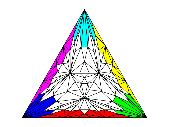
Figure 2. Categories of 2-simplices in $Ch^{2}(s^{2})$

Categories of 2-simplices in $Ch^{2}(s^{2})$

The first is a topological concept. We will use the definition of (Spa, 66). A simplicial complex is said to be homogeneously n-dimensional if every simplex is a face of some n-simplex of the complex. An n-dimensional pseudomanifold is defined to be a simplicial complex $\mathcal{K}$ such that

• $\mathcal{K}$ is homogeneously n-dimensional.

• Every $(n-1)$-simplex of $\mathcal{K}$ is the face of at most two n-simplices of $\mathcal{K}$.

• If $s$ and $s^{{}^{\prime}}$ are n-simplices of $\mathcal{K}$, there is a finite sequence $s=s_{1},s_{2},\cdots,s_{m}=s^{{}^{\prime}}$ of n-simplices of $\mathcal{K}$ such that $s_{i}$ and $s_{i+1}$ have an $(n-1)$ face in common for $1\leq i<m$.

There is a relation denoted by $s\sim s^{{}^{\prime}}$ in the set of n-simplices of a pseudomanifold defined by $s\sim s^{{}^{\prime}}$ if and only if there exists a finite sequence $s=s_{1},s_{2},\cdots,s_{m}=s^{{}^{\prime}}$ such that $s_{i}$ and $s_{i+1}$ have an $(n-1)$ face in common, as in condition (c). Obviously, this relation is a reflexive, symmetric, and transitive relation, and therefore an equivalence relation. An important property proved in (Spa, 66) is that any subdivision of a pseudomanifold is also a pseudomanifold.

The second concept is about a subcomplex of the $n$-th chromatic subdivision of a $k$-simplex. We define the non-boundary complex of $Ch^{n}(s^{k})$ as the simplicial complex consisting of those simplices in $Ch^{n}(s^{k})$, each vertex of which has a carrier $s^{k}$. In other words, the non-boundary complex can be obtained from $Ch^{n}(s^{k})$ by removing all those n-simplices that have some vertices in the boundary of $Ch^{n}(s^{k})$. In the example of $Ch^{2}(s^{2})$ shown in Figure 2, the non-boundary complex is the simplicial complex with white color. We want to sort the n-simplices of a non-boundary complex into a sequence. The following lemma proves that the non-boundary complex is a pseudomanifold.

Lemma 5.13.

The non-boundary complex of any iterated chromatic subdivision of a $k$-simplex is a pseudomanifold.

Proof.

Let $Ch^{n}(s^{k})$ be an iterated chromatic subdivision of a simplex $s^{k}$. We prove this by induction on the number $n$. If $n=1$, then the non-boundary complex has only one $k$-facet which is the central $k$-simplex of the chromatic subdivision, and therefore is a pseudomanifold.

Assume that the non-boundary complex of $Ch^{n-1}(s^{k})$ is a pseudomanifold. Then the chromatic subdivision of it will be a pseudomanifold. In other words, those simplices in the non-boundary complex of $Ch^{n}(s^{k})$ reached from some $k$-simplex in the non-boundary complex of $Ch^{n-1}(s^{k})$ are in one equivalence class. Any remaining $k$-simplex is reached from some so-called boundary $k$-simplex of $Ch^{n-1}(s^{k})$. Note that our definition of a boundary simplex is different from that of other materials.

Let $\sigma$ be a boundary $k$-simplex of $Ch^{n-1}(s^{k})$, then we will show that the non-boundary simplices of $Ch^{n}(s^{k})$ reached from $\sigma$ will be in the same equivalence class. Let $V$ denote the set of vertex of $\sigma$ consisting of those whose carrier is $s^{k}$. In other words, $V$ are those internal vertices of $\sigma$. Then there is a bijection $\rho$ between the partitions of $\Pi$ whose first process set contains some vertex in $V$ and the non-boundary simplices reached from $\sigma$. For each vertices set $S$ containing some vertex in $V$, $NBS(S)$ is defined to be $\{\rho(Par)\}$ where $Par$ is a partition of $\Pi$ and the first partition set is $S$. $NBS(S)$ is the joining of a $|S|$-simplex and the chromatic subdivision of a $(|\Pi|-|S|)$-simplex. Since the latter is a pseudomanifold, $NBS(S)$ is a pseudomanifold. For each vertex $v\in V$, $NBS(v)$ is defined as the union of all $NBS(S)$ where $v\in S$, as shown in Figure 3. The intersection between $\sigma\uparrow\{v\}$ and $\sigma\uparrow\{v\}\bigcup V^{{}^{\prime}}$, for some $V^{{}^{\prime}}\subseteq V$, is $(\Xi\downarrow\{v\})(\sigma\uparrow\{v\}\bigcup V^{{}^{\prime}})$. In other words, the intersection is a simplicial complex whose dimension is $(k-1)$. Therefore, all simplices of $NBS(v)$ belong to the same equivalence class. Each $NBS(v)$, where $v\in V$, contains $NBS(V)$ and therefore belongs to the same equivalence class. The set $\{NBS(v)\}$ forms a covering of non-boundary simplices of $Ch^{n}(s^{k})$ reached from $\sigma$, which are therefore in the same equivalence class.

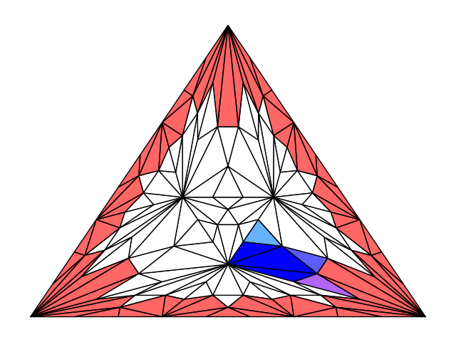
Figure 3. $NBS(v)$ in $Ch^{2}(s^{2})$

$NBS(v)$ in $Ch^{2}(s^{2})$

Then we will show that the equivalence class is the same regardless of which boundary $k$-simplex $\sigma$ of $Ch^{n-1}(s^{k})$ is chosen. All simplices in $Ch^{n-1}(s^{k})$ (including both non-boundary simplices and boundary simplices) form a pseudomanifold since $s^{k}$ is a pseudomanifold. If $s$ and $s^{{}^{\prime}}$ are k-simplices of $Ch^{n-1}(s^{k})$, by definition, there is a finite sequence $s=s_{1},s_{2},\cdots,s_{m}=s^{{}^{\prime}}$ of k-simplices of $Ch^{n-1}(s^{k})$ such that $s_{i}$ and $s_{i+1}$ have an $(n-1)$-face in common, for $1\leq i<m$. After a subdivision of the common $(n-1)$-face, the central simplex will be an internal $(n-1)$-face which is a common $(n-1)$-face of two non-boundary simplices reached from $s_{i}$ and $s_{i+1}$ respectively. Therefore, the non-boundary simplices reached from $s_{i}$ and $s_{i+1}$ are in the same equivalence class. We can get the same result for $s$ and $s^{{}^{\prime}}$, which means that there exists one unique equivalence class for all non-boundary simplices of $Ch^{n}(s^{k})$.

∎

5.2.5. Finalization after phase 1(Stage 3, 4)

We return to the discussion of different categories related to an intersection facet $s^{k}$. We will discuss the category whose carrier is $s^{k}$, and then the category whose carrier is some subsimplex $s^{k-1}$. Finally, an induction is given.

The first step is to consider the category whose carrier in $Ch(\mathcal{I})$ is the $k$-facet $s^{k}$. By Lemma 5.13, we know that the $k$-simplices in this category form a pseudomanifold. It is possible to enumerate these $k$-simplices in a finite sequence $s_{0},s_{1},....,s_{q},....s_{e}$ and to find a sequence $s_{1}^{{}^{\prime}},....,s_{q}^{{}^{\prime}},....$ of $(k-1)$-simplices of the internal complex such that for $q\geq 1$, $s_{q}^{{}^{\prime}}$ is a face of $s_{q-1}$ and also a face of $s_{q}$. Note that we only require every $k$-simplex to appear in this sequence, as a consequence of which a $k$-simplex may appear multiple times. The shared $k$-simplex that makes $s^{k}$ compatible is chosen to be the last $k$-simplex $s_{e}$ of the sequence.

The adversary will maintain a finalization invariant after processing the n-cliques whose projections are in $s_{q}$: for each set with some opposite label $(U^{{}^{\prime}},V^{{}^{\prime}})$ in the union of the n-cliques whose projections $prj(\sigma)$ are in $s_{0}\cup s_{1}\cup s_{2}....\cup s_{q}$, the outermost layer of the set can be expressed as the output configuration of $s_{q}$ using $Protocol(U^{{}^{\prime}},V^{{}^{\prime}})$. The problem is that the added layers of different output configuration may be adjacent to the same vertex whose output value is therefore impossible to decide. To avoid the conflict of terminated values in further induction, for those n-cliques whose projections have not appeared in $s_{0}\cup s_{1}\cup s_{2}....\cup s_{q}$, any undefined path between non-adjacent added layers should have a large length. This can be achieved by increasing the number of layers added when processing $s_{q}$.

Consider the n-cliques $\sigma$ whose projections $prj(\sigma)$ are in $s_{0}$. The adversary adds some layers of projection values $prj(\sigma)$ to each set. In fact, this is the first step for any terminated set, which will be repeated many times in the following discussion. Let $v$ be a terminated vertex with some opposite label $(U^{{}^{\prime}},V^{{}^{\prime}})$, and let $v^{{}^{\prime}}$ be some vertex adjacent to $v$. The adversary will terminate $v^{{}^{\prime}}$ with some value of the output configuration of $s_{0}$ using $Protocol(U^{{}^{\prime}},V^{{}^{\prime}})$. We require that if the id of $v^{{}^{\prime}}$ is in $s_{0}$, then it is terminated with the corresponding value. This rule should apply to any termination with projection values. The newly introduced output configurations are always valid since the task is colorless. For those n-cliques $\sigma$ whose projections $prj(\sigma)$ are a subsimplex of $s_{0}$, simply add layers of output configuration of the corresponding subsimplex of $s_{0}$. The finalization invariant holds.

The adversary then processes the n-cliques whose projections are in $s_{1}$. The terminated sets can be classified into three types: sets in n-cliques whose projections are in $s_{0}$, sets in n-cliques whose projections are in $s_{1}$, and sets at the intersection.

First, the adversary processes the sets in the n-cliques whose projections are in $s_{0}$: add some layers of output configurations of $s_{1}$ using $Protocol(U^{{}^{\prime}},V^{{}^{\prime}})$ to each set. This is possible since the output configuration of $s_{1}$ using $Protocol(U^{{}^{\prime}},V^{{}^{\prime}})$ is different from that of $s_{0}$ by the output value of only one vertex, denoted by $p$. Suppose that before the operation, $s^{n}$ is a $n$-simplex partially terminated with the output configuration of $s_{0}$. If $s^{n}$ has some terminated value of the process $p$, then the adversary terminates the remaining vertices of $s^{n}$ with the output configuration values of $s_{0}$ except the value of the process $p$, i.e. the values of $s_{1}^{{}^{\prime}}$. If $s^{n}$ does not have any terminated value of the process $p$, then the adversary terminates the remaining vertices of $s^{n}$ with values of the output configuration of $s_{1}$. The outermost layer will be the output configurations that contain values in the output configuration of $s_{1}$.

Then we consider the sets in the n-cliques whose projections are in $s_{1}$. The adversary adds some layers of projection values. In other words, the adversary terminates the vertices adjacent to a terminated vertex with values of $s_{1}$.

The remaining sets are those sets at the intersection of the n-cliques whose projections are in $s_{1}$ and those whose projections are in $s_{1}^{{}^{\prime}}$. That is, the projections of these sets will be in both $s_{0}$ and $s_{1}$. Again, the adversary adds some layers of projection values. If some newly terminated vertex is projected onto some simplex $s_{prj}$ in $s_{0}\cup s_{1}$, it is terminated with some value of the output configuration of $s_{prj}$. The adversary then adds some layers of $s_{1}^{{}^{\prime}}$. The outermost layer has output configurations of $s_{1}$ since $s_{1}^{{}^{\prime}}$ is a subsimplex of $s_{1}$. The adversary will add layers of $s_{1}$ to keep the finalization invariant true.

Suppose that the adversary has processed the n-cliques whose projections are in $s_{0}\cup s_{1}\cup....\cup s_{q-1}$ and the finalization invariant is true. The adversary processes the sets in the n-cliques whose projections are in $s_{q}$, which are divided into three types as above.

First, the adversary looks back to the sets whose projections are in $s_{0}\cup s_{1}\cup....\cup s_{q-1}$. Such a set can be in multiple n-cliques. The adversary adds some layers of output configurations of $s_{q}$, which is possible since the output configuration of $s_{q-1}$ is different from that of $s_{q}$ by the output value of only one vertex. Details have already been given in the discussion of $s_{1}$.

Then we consider the sets totally in the n-cliques whose projections are in $s_{q}$. The adversary adds layers of projection values. In other words, the adversary will terminate the vertices adjacent to a terminated vertex with some value of the output configuration of $s_{q}$.

The main obstacle is to add layers to the sets at the intersection of the n-cliques whose projections are in $s_{q}$ and those whose projections are in $s_{0}\cup s_{1}\cup....\cup s_{q-1}$. Now if $s_{q}$ has appeared in the sequence before it(remember that we do not require that a $k$-simplex appear only once in the sequence), then the adversary will treat these sets as sets whose projections are in $s_{0}\cup s_{1}\cup....\cup s_{q-1}$. The adversary adds some layers of output configurations of $s_{q}$.

If $s_{q}$ has not appeared in the sequence before it, the adversary has to deal with sets at the intersection. In the general situation, the boundary is not restricted to $s_{q}^{{}^{\prime}}$ as in the case of $s_{1}$ and this is the reason why the general discussion will be much more complicated. By the finalization invariant, for each terminated set in previous n-cliques, the outermost layer of it has the output configurations of $s_{q_{1}}$. If a set in the new n-cliques is connected to some previous set, then these sets should be merged into a single set. However, the existing added layers are not enough. This happens because some vertices on the previous boundary are no longer boundary vertices when the adversary processes more n-cliques. More specifically speaking, for a vertex $v_{o}$ after the second stage on the boundary of an $n$-clique $\sigma$ whose projection is in $s_{q}$ and an $n$-clique whose projection is in $s_{i}$ where $i<q$, the adversary has to terminate some vertices in $\sigma$ reached from $v_{o}$ to ensure that the internal layers of the existing added layers to $v_{o}$ will not be exposed. Will this operation cause any conflict of assigned values in these n-cliques whose projections are in $s_{q}$? Will the operation terminate more vertices on the boundary so that the adversary has to look back to $s_{i}$ to fix the same problem? Before we present what the adversary will do, we have to analyze the terminated sets.

After the first stage, in which enough chromatic subdivisions are made, the sets in an n-clique will either have a large active distance to the boundary of the n-clique or have a zero active distance. Sets of the former type have been discussed and will not affect the merging of sets. The sets we are more interested in belong to the latter type, which means that after the second stage the set will contain some terminated vertices on the boundary and the sets from different n-cliques should be merged into a single one. These terminated vertices on the boundary have output configurations of $s^{q}$. And some layers have already been added to them on the boundary.

It is quite natural to think that the adversary can add layers to the merged set using the values of the existing added layers on the boundary. But this method does not work for our current adversarial strategy. Suppose that the dimension of $s_{q}$ is $k$, a boundary simplex of $s_{q}$ is defined as a subsimplex of $s_{q}$ whose dimension is $(k-1)$. This idea will not work for sets containing vertices whose projections are in different boundary simplices of $s_{q}$. In other words, a set can be connected to many existing terminated sets, each of which is in the n-cliques whose projections are in $s_{j_{i}}$ where $j_{i}<q$. Recall that the intersection simplex can be terminated with an opposite label and is not restricted by the assignment rule (2) since the terminated configuration of such a simplex is one of its possible configurations. There will be multiple choices of the existing added layers that cause a conflict of output values to be used.

The solution to this disturbing issue is that we should limit the usage of the existing added layers in a boundary simplex of $s_{q}$ to the undefined vertices near it, rather than those vertices near another disjoint boundary simplex. To achieve this goal, we have to reconstruct our adversarial strategy described in Section 5.2.2. We place a restriction on the termination of a vertex with some protocol configuration, just as on the termination with opposite configuration. Once the adversary terminates a vertex with its protocol configuration, it can not do it again until several rounds later. This restriction can only cause a liveness issue which has been shown to be impossible by Lemma 5.12 in the previous setting. However, as the proof of Lemma 5.12 shows, the restriction on the second assignment rule will not cause an infinite chain of queries. Due to the same reason, the new rule of termination with protocol configurations will not cause an infinite chain of queries, i.e., lead to a liveness problem. Perhaps we have to explain to the readers why this rule is not introduced in Section 5.2.2. We impose a restriction on the second assignment rule, since the definition of opposite cliques with the label $(U,V)$ can only be used for those n-cliques having an intersection with $Input(U,V)$. But this is not the situation for those vertices terminated with some of its possible configurations. The new rule will limit the projection of a terminated set to the open star of some simplex on the boundary. Therefore, the adversary can terminate the undefined vertices near the set using the values of the existing added layers on the boundary without conflicts.

In our adversarial strategy, any vertex $v$ in an n-clique $\sigma$ terminated with some opposite label $(U^{{}^{\prime}},V^{{}^{\prime}})$ will be connected to some boundary vertex $v_{b}$ with $Input(U^{{}^{\prime}},V^{{}^{\prime}})$. The n-clique $\sigma$ can be seen as the joining of a boundary simplex $\sigma_{b}$ and a non-boundary simplex $\sigma_{nb}$. Let $Carrier(v_{b},\sigma_{b})$ denote the carrier of $v_{b}$ in $\sigma_{b}$.

Lemma 5.14.

The carrier of a vertex $v$ not in $\sigma_{b}$ will be the joining of $Carrier(v_{b},\allowbreak\sigma_{b})$ and $\sigma_{nb}$, or a larger simplex that contains it.

Proof.

We will prove this result by contradiction. Suppose that the carrier of $v$ in $\sigma$ is the join of any strict subsimplex of $Carrier(v_{b},\allowbreak\sigma_{b})$ and $\sigma_{nb}$, denoted by $\sigma_{des}$. There exists a shortest path $v_{0}=v_{b},v_{1},....v_{e}=v$ from $v_{b}$ to $v$. The vertex $v_{0}$ is not in $\sigma_{des}$ and $v_{0}$ is not adjacent to $v_{e}$ since $v_{e}$ is not a vertex in $\sigma_{b}$. We know $e>1$. Both $v_{e-1}$ and $v_{e}$ are undefined vertices when $v_{e-2}$ is terminated. When $v_{e-1}$ is terminated after $r_{spe}$ rounds, there will be some undefined vertices between $v_{e-1}$ and $v_{e}$, which is a contradiction. ∎

Although we do not use the second assignment rule to add layers to the terminated sets, the number of added layers has an upper bound, which means that if enough subdivisions are made in the first stage, the added layers will also satisfy the above lemma. Now, considering the vertices of a terminated set after the second stage in $\sigma_{b}$, we will prove that these vertices will be in the open star of some subsimplex of $\sigma_{b}$. In other words, we will prove that there exists a terminated vertex whose carrier is $C_{a}$ such that each terminated vertex will have a carrier containing $C_{a}$.

Lemma 5.15.

Let $\sigma$ be an $n$-clique in $Ch^{r_{max}}(\mathcal{I})$. For each terminated set after the second stage in $\sigma_{b}$, there exists a terminated vertex whose carrier is $\sigma_{a}$ such that each terminated vertex will have a carrier containing $\sigma_{a}$.

Proof.

Suppose that the carriers of two terminated vertices in $\sigma_{b}$ share a common simplex $s_{s}$ in $\sigma_{b}$ but that no terminated vertex in $\sigma_{b}$ has a carrier $s_{s}$, then the two vertices are connected by a terminated path, each vertex having zero active distance to $s_{s}$. By our adversarial strategy, some vertices in the subdivision of $s_{s}$ will terminate in the second stage, which is a contradiction. ∎

Now we return to the discussion of n-cliques whose projections are in $s_{q}$. Suppose that a terminated set $V_{t}$ merges with a previous set $V_{p}$. We have to define a set of vertices in $V_{t}$ after the second stage. Let $V_{o}$ be a set of vertices in $V_{t}$ on the boundary with $V_{p}$. Then $V_{o}$ is a subset of $V_{t}$. Recall that a boundary simplex of $s_{q}$ is a subsimplex of $s_{q}$. The adversary will use the existing layers added to $V_{o}$ to terminate some vertices reached from $V_{t}$ whose projections are in $s_{q}$ but not in $s_{q}^{{}^{\prime}}$.

If the projection of $V_{o}$ is within some boundary simplex of $s_{q}$, the adversary will use the existing layers added to $V_{o}$. First, the adversary adds layers of projection values to $V_{t}$. Let $V_{t}^{{}^{\prime}}$ denote the newly terminated vertices. The difference here is that the adversary uses the output configuration of the boundary simplex, rather than that of $s_{q}$. The adversary can then add layers compatible with the existing layers on the boundary: for each vertex $v$ in $V_{t}^{{}^{\prime}}$, the adversary terminates the vertices reached from $v$ by an undefined path whose length equals the number of existing layers. The concrete values are obtained from the existing terminated layers added to $V_{o}$ on the boundary.

Layers added to a vertex in $V_{t}$ will not reach a vertex on the boundary. This is true even for those vertices that are adjacent to a terminated vertex on the boundary after the second stage. Suppose that after the second stage, $v_{0}$ is a terminated vertex on the boundary and $v_{1}$ is a terminated vertex not on the boundary. The two vertices are both undefined vertices after the first stage. Let $\sigma$ denote an undefined $n$-simplex containing $v_{0}$ and $v_{1}$ before stage 1. Note that at this time, $v_{1}$ may not exist in $S^{t}$. The simplex $\sigma$ will be subdivided using the standard chromatic subdivision enough times so that the active distance from $v_{1}$ to the boundary will be 1 or a large number. So, after the second stage where $v_{0}$ and $v_{1}$ are terminated, any path consisting of undefined vertices from $v_{1}$ to a vertex on the boundary will have a long length. We give a simple example to present our idea in Figure 4. When the adversary merges the sets on the boundary, the added layers to $v_{1}$ will not reach the boundary, which means that the adversary will not have to change the already terminated vertices on the boundary or terminate some new vertices on the boundary. Therefore, the adversary will not alternate infinitely between different sides of the boundary, and it is valid for us to choose the form of induction to process the terminated sets.

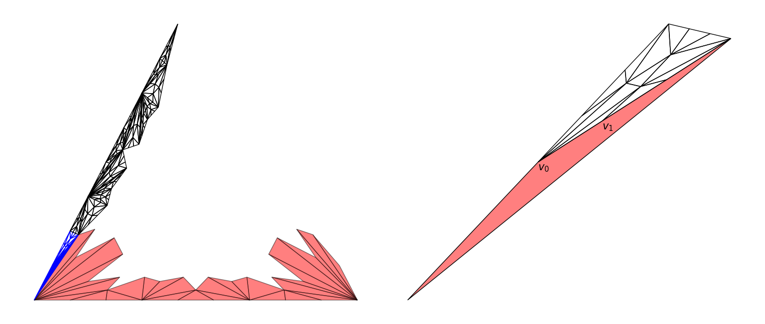
Figure 4. $v_{1}$ will have a large distance to the boundary

$v_{1}$ will have a large distance to the boundary

A more complicated situation is that the projection of $V_{o}$ will be in multiple boundary simplices. More than one type of existing layer has been added to $V_{o}$. At first, each vertex of the merged set will be mapped to a projection vertex in $V_{o}$. This can be done by projecting a vertex $v$ to $\sigma_{b}$ and then to boundary simplices. This is even valid for those vertices whose projections are in some boundary simplex of $s_{q}$ which is not a shared boundary simplex with $s_{0}\cup s_{1}\cup....\cup s_{q-1}$. Still, the adversary has to add layers consisting of terminated values of the boundary simplices. The terminated value of a vertex adjacent to some vertex $v$ will be the output value of the projection vertex of $v$. Since there will be some vertex $V_{sh}$ in $V_{o}$ terminated in the shared simplex of two boundary simplices by Lemma 5.15, the terminated values added to the vertices whose projection vertices are in $V_{sh}$ will serve as the intermediate part. Therefore, the newly terminated vertices will not have any conflict of output values. Let $V_{t}^{{}^{\prime}}$ denote the newly terminated vertices. The adversary can add layers compatible with existing terminated vertices: for each terminated vertex $v$ in $V_{t}^{{}^{\prime}}$, the adversary can terminate the vertices reached from $v$ by an undefined path whose length equals the number of existing added layers to its projection vertex. Concrete values are also obtained from the existing terminated layers added to its projection vertex on the boundary. Different types of added layers will not cause any conflict since the existing added layers on the boundary do not have a conflict of values. The output configurations of the outermost layer are those of $s_{q-1}$. Finally, the adversary will add some layers of $s_{q}$. All the added layers mentioned above will not cause any violation of the task specification, since we are discussing the n-cliques in the same category and the finalization invariant still holds.

By induction, finally the adversary will process the last $k$-simplex in the sequence, i.e. the shared $k$-simplex. By the finalization invariant, the output configurations of the outermost layer only contain values of the shared output configuration of $Protocol(U,V)$ and $Protocol(U^{{}^{\prime}},V^{{}^{\prime}})$. From now on, these shared output configurations will be seen as output configurations with the label $(U,V)$.

The adversary will add more layers to connect the shared output configuration to each output configuration in the n-cliques by $Protocol(U,V)$, dual to what it has done. This time, the adversary will reverse the sequence of k-simplices as $s_{e},s_{e-1},....,s_{q},....s_{0}$. When processing $s_{q}$, the adversary will add some layers of output configurations of $s_{q}$ using $Protocol(U,V)$ to all sets in the n-cliques whose projections are in $s_{q}\cup s_{q+1}...\cup s_{0}$. If the projection of a set is both in $s_{e}\cup s_{e-1},....\cup s_{q+1}$ and $s_{q}\cup s_{q+1}...\cup s_{0}$, the new added layers will be applied to those vertices whose projections are in $s_{q}\cup s_{q+1}...\cup s_{0}$ while leaving the other vertices untouched.

After the adversary processes $s_{0}$ in this way, we will discuss the sets in the n-cliques whose projections are in $s_{q}$. If a set is completely contained in these n-cliques, then the outermost layer of the set will be the output configuration of $s_{q}$ using $Protocol(U,V)$, which is exactly what we want. The sets whose projections are on the boundary of $s_{q}$ can be divided into two types. If a set is on the boundary with the n-cliques whose projections are in $s_{q+i}$ for some integer $i$, then the outermost layer of the set will be the output configurations of $s_{q}$. But if a set is on the boundary with the n-cliques whose projections are in $\sum s_{q-i}$ for a set of integers $i$, then some new terminated vertices reached from $V_{o}$ will be exposed as the outermost layer in the n-cliques whose projections are in $s_{q}$. The adversary uses the same techniques as described in the previous paragraphs. To accommodate these newly terminated vertices on the boundary, the adversary can add layers by assigning values to the undefined vertices reached from some vertex in $V_{t}^{{}^{\prime}}$ by an undefined path whose length equals the number of layers added to its projection vertex. The outermost layer consists of protocol configurations of $s_{q}$, since the protocol configurations of two adjacent cliques are the same on their shared boundary.

The last step is to add some layers to ensure that if some vertex $v$ of the outermost layer is projected onto some simplex in the subdivision of $s^{k}$, then it will use some value of the protocol configuration of this simplex as its output. This is always possible by adding vertices of the required output values directly, since the task is colorless. The reason for introducing this step is explained in the following discussion.

The adversary now processes the categories whose carriers are facets of the $(k-1)$-skeleton of $s^{k}$, denoted by $s^{k-1}$. These categories will not overlap, as indicated by the red, purple, and yellow colors in Figure 2. This can be proved by the active distances between their carriers. However, each of these categories may have a shared boundary with the category whose carrier is $s^{k}$. Before the adversary repeats what it has done to the category whose carrier is $s^{k}$, it has to deal with those vertices on the boundary with the n-cliques whose projections are in $s^{k}$. Note that the boundary between different categories is not simply a simplex like the boundary of their projections in $s^{k}$, but contains each n-clique whose projection is within the boundary of their projections. As the reader can see, the adversary uses similar techniques again. Stage 1 and stage 2 are the same as in the previous category(including how many times the chromatic subdivisions are made). In fact, what we have done is to bring stage 1 and stage 2 of all categories forward to merge into single stage 1 and stage 2.

Since the adversary has processed the category whose carrier is $s^{k}$, some n-cliques in the category whose carrier is $s^{k-1}$ will see some newly terminated layers on the boundary. The outermost layer consists of values of protocol configurations. But our procedure requires that, at the beginning, the outermost layer consists of the output configurations of the opposite clique with the label $(U^{{}^{\prime}},V^{{}^{\prime}})$ (rather than the protocol configurations). The adversary will add layers compatible with existing layers by assigning values to those undefined vertices reached from some terminated vertex after the second stage by an undefined path whose length equals the number of needed layers, similar to what the adversary has done so many times. However, to recover the output configuration of the opposite label $(U^{{}^{\prime}},V^{{}^{\prime}})$, the adversary will add the same set of layers, but in reverse order. A key observation is that for each terminated set in the n-cliques of the category whose carrier is $s^{k-1}$, if it has some vertices on the boundary with the category whose carrier is $s^{k}$, then the carrier of projections of this set is $s^{k}$ rather than any subsimplex of $s^{k}$. By Lemma 5.14, the added layers will not violate the carrier map.

Now, the required conditions of our procedure are satisfied. The adversary will use techniques for the category with carrier $s^{k}$. As a consequence, the outermost layer of the sets with the label $(U^{{}^{\prime}},V^{{}^{\prime}})$ will be the protocol configurations of its projections. Note that the projections here are projections to the carrier of the category, that is, $s^{k-1}$ rather than $s^{k}$. Therefore, a vertex shared by two categories can be projected onto different simplices in the subdivision of $s^{k}$. To avoid any conflict of output values, the last step is to add some layers to ensure that if a vertex of the outermost layer is projected onto some simplex in the subdivision of $s^{k}$, it will use some value from the protocol configuration of this simplex as its output. This is possible since the task is assumed to be colorless.

After the procedure for a category, the layer addition operation will now be used for those n-cliques in the category whose carrier is $s^{k}$ to eliminate the impacts of the current category. After this, the outermost layers of the sets with the label $(U^{{}^{\prime}},V^{{}^{\prime}})$ in n-cliques of the category with carrier $s^{k}$ will still be their protocol configurations.

A general induction can be given. Suppose that the categories whose carriers are facets of the $k-q+1$-skeleton of $s^{k}$ for some $0<q\leq k$ have been processed and the outermost layer of the sets with the label $(U^{{}^{\prime}},V^{{}^{\prime}})$ in the n-cliques of those categories will be their protocol configurations. Let $s^{k-q}$ be the carrier of some category. Then it has some shared boundary with some previous categories. To create the required conditions of our procedure, the adversary has to add layers compatible with newly terminated vertices. The new assigned values are obtained from the existing layers on the boundary. The adversary then adds layers in reverse order to recover the output configuration of the opposite label $(U^{{}^{\prime}},V^{{}^{\prime}})$. Now, the procedure for a category will be used. To avoid conflict of output values, some layers are added to ensure that if a vertex of the outermost layer is projected onto some simplex in the subdivision of $s^{k}$, it will use some value from the protocol configuration of this simplex as its output. Finally, the operation of adding layers will be used in previous categories to eliminate the impacts of the current category. No task specification will be violated, as we have shown for the category whose carrier is $s^{k-1}$. Until now, we have processed categories, each of which has a carrier of a subsimplex of a $k$-facet.

In fact, the idea of alternating between protocol configurations and output configurations of opposite cliques on the boundary will also be used to connect the categories of different k-facets, including k-facets reached from different initial configurations. We remind the reader that the input complex $Input(U,V)$ contains all configurations in $Ch^{1}(\mathcal{I})$ reached from some initial configuration in which the processes in $V$ satisfy the value requirement $V$. The complex of intersections of $Input(U,V)$ and $Input(U^{{}^{\prime}},V^{{}^{\prime}})$ in $Ch^{1}(\mathcal{I})$ can contain $k$-facets reached from different initial configurations. But there is some risk of safety problems. We have to show that the terminated values used in alternating will not cause a violation of the carrier map. In short, the output configurations the adversary will use in alternating are all obtained from the already terminated layers on the boundary of two categories, and the vertices to be terminated will have a larger or equivalent carrier.

We will use Lemma 5.14 to the shared boundary of two categories. Suppose that two categories are adjacent and that the vertex $v_{o}$ in an $n$-clique $\sigma$ is on the shared boundary of two categories after the second stage. The existing layers added to $v_{o}$ have a carrier as the join of $Carrier(prj(v_{o}),Ch(\mathcal{I}))$ and $\sigma_{nb}$. The projection of the newly terminated vertices has a carrier containing $Carrier(prj(v_{o}),Ch(\mathcal{I}))$. The newly terminated vertices reached from $v_{o}$ have a larger carrier than(or an equal carrier as) the join of $Carrier(prj(v_{o}),\mathcal{I})$ and $\sigma_{nb}$. Therefore, the existing layers to $v_{o}$ on the boundary can be used without any violation of the task specification.

Finally, after processing all intersection facets of all possible opposite labels $(U^{{}^{\prime}},V^{{}^{\prime}})$, the adversary arrives at stage 4 where it will fill the gap between the sets of different labels. By our construction, the outermost layers of the sets with label $(U^{{}^{\prime}},V^{{}^{\prime}})$ in each n-cliques of each category will be their protocol configurations. Therefore, the adversary uses the value of the protocol configuration for each undefined vertex $v$ in $S^{t}(\sigma)$ for each n-clique $\sigma$ in $Ch^{r_{max}-1}(C)$ where $C\in Input(U,V)$. Each vertex in $S^{t}$ reached from $Input(U,V)$ has been terminated with an output value, which means that the adversary has constructed a protocol for $Input(U,V)$. In phases $\varphi\geq 2$, the adversary will respond to queries according to the protocol and therefore will not cause safety or liveness problems. Eventually, the prover will choose a configuration in which every process has terminated to end some phase and lose in the next phase.

We summarize the above results into a theorem.

Theorem 5.16.

For a general colorless task$(\mathcal{I},\mathcal{O},\Delta)$, there exists an adversary that can finalize after the first round to win against any restricted extension-based prover if and only if there exists a protocol for each $Input(U,V)$ and all intersection simplices in the standard chromatic subdivision of all initial configurations are compatible.

5.3. Augmented extension-based proofs

Now we consider augmented extension-based proofs that allow assignment queries $(C,P,f)$. The prover has to reply whether there exists a $P$-only schedule from the configuration $C$ such that the output values of $Q\subseteq P$ satisfy the requirement of $f$. The prover can submit assignment queries to obtain all possible output configurations reached from a $k$-simplex $s^{k}$ in $Ch(\mathcal{I})$ at the intersection of $\Xi(C\uparrow U_{1})$ and $\Xi(C\uparrow U_{2})$. Then after the first phase, the output configurations for a $k$-simplex reached from $s^{k}$ by the protocols constructed for $Input(U_{1},V_{1})$ and $Input(U_{2},V_{2})$ should be these configurations. Will this new type of query give the prover more power and a stronger condition for finalization be required? The answer to this question is no. In this section, we will show that the adversary can answer the assignment queries while maintaining the invariants and guaranteeing that the response of augmented extension-based proof will not be violated.

For each n-clique $\sigma$ in $Ch^{r_{max}}(\mathcal{I})$, any possible terminated configuration in $S^{t}(\sigma)$ after phase 1 is a subsimplex of the protocol configuration of $\sigma$, a subsimplex of the output simplex of its opposite clique with $(U^{{}^{\prime}},V^{{}^{\prime}})$, or a subsimplex of some output configuration introduced in finalization, as described in Sections 5.2.4 and 5.2.5. In previous sections, we have not discussed the configurations introduced in finalization, since the proof of correctness will not depend on the concrete values of output configurations. But now to answer the assignment queries, we have to look into the details.

For each n-clique $\sigma^{{}^{\prime}}$ in the same category, let $prj(\sigma^{{}^{\prime}})$ denote the projection of $\sigma^{{}^{\prime}}$ into the carrier of the category. The newly terminated configurations in $\sigma$ will contain output configurations whose values are chosen from the protocol configuration or the output configuration of the opposite clique of $prj(\sigma^{{}^{\prime}})$. We define the finalization configurations of a category as these output configurations, since they are shared by each n-clique $\sigma$ in the category. But this is not enough for those n-cliques on the boundary with other categories. We have to analyze this in a more fine-grained way. For each n-clique $\sigma$ in $Ch^{r_{max}-1}(Input(U,V))$, let $s^{l}$ denote a $l$-simplex with the label $(U^{{}^{\prime}},V^{{}^{\prime}})$ reached from $\sigma$. By invariant (2), we know that there exists a terminated path from some $v_{o}$ on the boundary with other categories to $s^{l}$. The finalization configurations of $s^{l}$ will also contain the restrictions to the processes in $s^{l}$ of the finalization configurations of each category that contains the vertex $v_{o}$.

By our adversarial strategy described in Sections 5.2.4 and 5.2.5, the finalization configurations of the $l$-simplex $s^{l}$ in $\sigma$ will contain each possible output configuration of $s^{l}$. Note that we do not require each finalization configuration of $s^{l}$ to appear as a terminated configuration in stage 3 when the adversary is constructing a protocol for $Input(U,V)$. We will show that each finalization configuration of $s^{l}$ will not cause any violation of the task specification. If the category $C$ contains the n-clique $\sigma$, the finalization configurations of this category will not cause any violation of the task specification according to the definition of a category. If the category $C$ that contains the vertex $v_{o}$ does not contain $\sigma$, there exists a terminated path from $v_{o}$ to $s^{l}$. We can see the finalization configurations of $C$ as the existing layers added to $v_{o}$ on the boundary, and therefore these output configurations will not cause any violation of the task specification when applied to $s^{l}$, as we have shown that alternating between the protocol configurations and the output configurations of opposite cliques will not cause a safety issue. An important property of finalization configurations is that the space formed by all finalization configurations is a connected space. In other words, each finalization configuration can be connected to the output configuration of the opposite clique of $s^{l}$ by some path of finalization configurations, since the carrier of each category is compatible by assumption.

Suppose that the invariants hold before an assignment query $(C,P,f)$ in phase 1 and $C$ is reached from some configuration in $Input(U,V)$. By invariant (1), we know that the states of processes in $P$ will correspond to a simplex in $S^{r}$, where $r\leq t$. If the round number $r$ is less than $r_{max}$, the result of a single assignment query $(C,P,f)$ can be generated from the results of a set of assignment queries $(C^{{}^{\prime}},P,f)$ where $C^{{}^{\prime}}$ is a $k$-simplex reached from $C$ in $Ch^{r_{max}}(\mathcal{I})$. Therefore, we will only discuss the assignment queries where $r\geq r_{max}$ and the configuration $C$ is reached from some n-clique $\sigma$ in $Ch^{r_{max}}(\mathcal{I})$. Let $R^{t}$ denote the subcomplex of $S^{t}$ consisting of all simplices $s^{k}$ reached from this simplex by a $P$-only $(t-r)$-round schedule. We will discuss the k-simplices in $R^{t}$.

Analysis is relatively straightforward when a desired configuration has already been reached or when all configurations are determined but no desired configuration has been reached. Note that the output configuration here is the protocol configuration or the output configuration of the opposite clique(not including the finalization configurations). If there exists a $k$-simplex $\tau$ in $R^{t}$ having some vertex $v$ terminated with label $(U^{d},V^{d})$ and the output configuration with label $(U^{d},V^{d})$ satisfies $f$, then the adversary can submit a chain of queries from this $\tau$ to itself. By Lemma 5.12 this chain of queries must be finite and end with a $(k-1)$-simplex with label $(U^{d},V^{d})$. The output values of the join of this simplex and $v$ satisfy $f$. Because the adversary does not change $\Delta$ and will not change the defined values once they have been set, the invariants will still hold. If each $k$-simplex $\tau$ in $R^{t}$ has some terminated vertices and the output configuration of this label $(U^{t},V^{t})$ does not satisfy the requirement of $f$, then no $k$-simplex reached from $\tau$ will satisfy $f$. This is because in the second stage of Section 5.2.4, each vertex adjacent to a terminated vertex will be terminated with the same label. Each $k$-simplex reached from $\tau$ will terminate with the output configuration with the label $(U^{t},V^{t})$.

Therefore, we will only discuss the $k$-simplices in $R^{t}$ that do not have a terminated vertex and $R^{t}$ contains at least one undefined $k$-simplex. For each undefined $k$-simplex $\tau\in R^{t}$, let $A_{\tau}$ denote the subcomplex of $S^{t}$ that contains vertices at a distance of at most 1 to each vertex in $\tau$. In other words, $A_{\tau}$ consists of all n-simplices that contain $\tau$. We will classify the different $\tau$ into several cases according to the status of the vertices of $A_{\tau}$. In cases 1 and 2, some vertices of $A_{\tau}$ have been terminated. These two situations are quite similar to the situation in which a vertex in $\tau$ is terminated. Therefore, the argument given in the last paragraph will be used again, and no finalization configurations are involved. In cases 3 and 4, all the vertices in $A_{\tau}$ are undefined. In case 3 where the surrounding vertices of $\tau$ are not defined, we will show that $\tau$ will be separated from other terminated sets. By invariant (2), the output configurations reached from $\tau$ are the finalization configurations with $b$, where $b$ is some possible label of some subset of $\tau$. In case 4, some vertex in $\tau$ is adjacent to a terminated vertex with the label $(U^{d},V^{d})$. Therefore, in addition to the finalization configurations with $b$, where $b$ is some possible label of some subset of $\tau$, the finalization configurations with the label $(U^{d},V^{d})$ are also possible.

Case 1: There is a $k$-simplex $\tau$ in $R^{t}$, some vertex in $A_{\tau}$ is terminated with the label $(U^{d},V^{d})$ and the output configuration with the label $(U^{d},V^{d})$ satisfies $f$. The adversary will submit a chain of queries such that some $k$-simplex reached from $\tau$ will terminate with the desired output configuration that satisfies the function $f$. Let $(U,v)$ be the protocol label and let $(U^{{}^{\prime}},V^{{}^{\prime}})$ be some opposite label. We choose to use the query chain to accommodate both cases: $(U^{d},V^{d})$ = $(U,V)$ or $(U^{d},V^{d})$ = $(U^{{}^{\prime}},V^{{}^{\prime}})$ as queries will not violate the invariants. The adversary can return the schedule from configuration $C$ to this $k$-simplex.

Case 2: There is a $k$-simplex $\tau$ in $R^{t}$ and some vertex in $A_{\tau}$ is terminated with a label $(U^{d},V^{d})$, but the projection into $P$ of the output configuration with the label $(U^{d},V^{d})$ does not satisfy $f$. Any simplex in a subdivision of $\tau$ will be adjacent to this terminated vertex. In stage 2 of Section 5.2.4, each undefined vertex adjacent to a terminated vertex will be terminated with its label. Therefore, all configurations reached from the $k$-simplex $\tau$ will have the label $(U^{d},V^{d})$ and are therefore not possible to satisfy the function $f$.

Case 3: There is a $k$-simplex $\tau$ in $R^{t}$, every vertex in $A_{\tau}$ is undefined and all vertices adjacent to $\tau$ are undefined.

Case 3.1: If the label $(U,V)$ is a possible label for $\tau$ and the projection into $P$ of the output configuration with the label $(U,V)$ satisfies $f$, the adversary can subdivide $S^{t}$ and increase $t$ three times. We define the simplex $\rho=\{(i,\vec{\tau}):i\in Id(\tau)\}$ in $Ch(\tau)$ as the central simplex of the standard chromatic subdivision. Then the central simplex of $Ch^{3}(\tau)$ will have an active distance of at least 3 to all terminated configurations with other labels. The adversary can terminate a simplex reached from this central simplex with the label $(U^{d},V^{d})$ and return the schedule from $C$ to this simplex.

Case 3.2: The discussions in case 3.1 are also true when $(U^{{}^{\prime}},V^{{}^{\prime}})$ is a possible label for only a subset $\tau^{{}^{\prime}}$ of $\tau$. If the output configuration with label $(U^{{}^{\prime}},V^{{}^{\prime}})$ satisfies the function $f$, the adversary will still subdivide $S^{t}$ and increase $t$ three times. In fact, any simplex in $Ch^{3}(\tau)$ will have an active distance of at least 3 to all terminated configurations with other labels. We will choose a simplex $s_{int}$ in $Ch^{3}(\tau)$ that has some subsimplex in $\tau^{{}^{\prime}}$. The adversary can then terminate a simplex reached from $s_{int}$ with the label $(U^{d},V^{d})$ and return the schedule from $C$ to this simplex.

Now, we have to discuss the output configurations introduced in the finalization. If some finalization configuration $s_{o}$ of $\tau$ with the label $(U^{{}^{\prime}},V^{{}^{\prime}})$ satisfies the function $f$, then the adversary will construct $s_{o}$. First, the adversary will construct a simplex $s_{int}$, as in the last paragraph. By the property of finalization configurations, the adversary can construct a path $l$ from $s_{int}$ to the desired configuration $s_{o}$ using rule (2). The adversary will ensure that the configuration $s_{o}$ is far enough from other terminated sets. The adversary has constructed the output configuration $s_{o}$ that satisfies the function $f$. But it can not stop here since it has terminated some vertices with label $(U^{d},V^{d})$ but not with the values of opposite clique with label $(U^{d},V^{d})$, while this is the most basic assumption of our interaction progress of extension-based proofs. The adversary will terminate the vertices reached from the simplex $s_{o}$ by a path $l$ such that the outermost layer of the terminated vertices will be the output configuration of the opposite clique. This is possible since each $n$-simplex containing $\tau$ is included in $A_{\tau}$. After this operation, the output configurations on the path from $s_{int}$ to $s_{o}$ will be sealed. The adversary will return the schedule from $C$ to the configuration $s_{o}$. Since we have constructed a path to any terminated simplex, invariant (2) will remain true.

Case 3.3: For each possible label $(U^{{}^{\prime}},V^{{}^{\prime}})$ of any subset of $\tau$, the projections to $P$ of all finalization configurations with label $(U^{{}^{\prime}},V^{{}^{\prime}})$ do not satisfy the function $f$. Even if the projection to $P$ of the output configuration with an opposite label $(U^{{}^{\prime}},V^{{}^{\prime}})$ satisfies the function $f$, the adversary cannot simply terminate some simplex reached from $\tau$ with the label $(U^{{}^{\prime}},V^{{}^{\prime}})$ since the adversary has to maintain the invariant (2) which says that there must be a terminated path to some existing simplex with the label $(U^{{}^{\prime}},V^{{}^{\prime}})$. However, it is not safe to say that there will be no simplex that is reached from $\tau$ and terminated with such a label $(U^{{}^{\prime}},V^{{}^{\prime}})$, and therefore satisfies the function $f$. In fact, there may be more possibilities, such as finalization configurations. In previous work (AAE⁺, 19), the adversary will terminate all vertices reached from $\tau$ with their protocol configurations to eliminate ambiguity. If we adopt their method, it will look like this: since all vertices in $\tau$ are not adjacent to the terminated vertices, the active distance between $\tau$ and every terminated configuration is at least 1. The adversary can subdivide $S^{t}$ and increase $t$ three times so that all simplices reached from $\tau$ have an active distance of at least 3 to any terminated configuration. The adversary will terminate all vertices with the label $(U,V)$ to ensure that they do not terminate with the label $(U^{{}^{\prime}},V^{{}^{\prime}})$ in the later interaction. But this method does not work for our adversarial strategy, since it can generate a set that is too large to contain all vertices in the subdivision of an intersection $k$-facet. Recall that in Section 5.2.5, we introduce a new rule for terminating a vertex with its protocol configuration. We will prove that any simplex reached from $\tau$ will not terminate with label $(U^{{}^{\prime}},V^{{}^{\prime}})$ using the restriction of the second assignment rule.

If some $k$-simplex reached from $\tau$ is terminated with the label $(U^{{}^{\prime}},V^{{}^{\prime}})$, the adversary has to find a terminated path from the exterior of $A_{\tau}$ to $\tau$. We will prove that this path is impossible and therefore all configurations reached from the $k$-simplex $\tau$ will not have the label $(U^{{}^{\prime}},V^{{}^{\prime}})$. Let $S_{\tau}$ denote the simplices in $S^{t}$ consisting of vertices that are adjacent to some vertex in $\tau$ but are not included in $\tau$. The vertices of $S_{\tau}$ are undefined by assumption. We will prove by contradiction that it is impossible for any vertex $v$ in the subdivision of $\tau$ to have the label $(U^{{}^{\prime}},V^{{}^{\prime}})$. The key idea of the proof is that the vertices of $\tau$ and the vertices terminated with $(U^{{}^{\prime}},V^{{}^{\prime}})$ in $S^{t}$ are separated by $S_{\tau}$. The restricted application of rule 2 will only increase the distance in further subdivisions.

Assume that the vertex $v_{n}$ is the first vertex in the subdivision of $\tau$ terminated with the label $(U^{{}^{\prime}},V^{{}^{\prime}})$. Then there exists an earliest path $v_{0},v_{1},....v_{n}$ from some vertex $v_{0}$ in the subdivision of $S_{\tau}$ to $v_{n}$. Consider the moment when the vertex $v_{n-2}$ is terminated in some $S^{t}$, $v_{n-1}$ is undefined. The active distance between $v_{n-2}$ and the subdivision of $\tau$ is at least 2. Let $S_{\tau}^{{}^{\prime}}$ denote the simplices of the current $S^{t}$ consisting of vertices that are adjacent to some vertex in the subdivision of $\tau$, but are not included in the subdivision of $\tau$. The vertices of $S_{\tau}^{{}^{\prime}}$ are not terminated with the label $(U^{{}^{\prime}},V^{{}^{\prime}})$, since the path we are discussing is the earliest path according to hypothesis. Therefore, $v_{n-1}$ must be in the subdivision of $S_{\tau}^{{}^{\prime}}$ and $v_{n}$ must be in the subdivision of $\tau$. After at least $r_{spe}$ rounds, any undefined path from the subdivision of $S_{\tau}^{{}^{\prime}}$ to the subdivision of $\tau$ will have a long length. It is not possible to terminate the vertex $v_{n}$ adjacent to $v_{n-1}$ with the label $(U^{{}^{\prime}},V^{{}^{\prime}})$. A configuration reached from the simplex $\tau$ is not possible to terminate with the label $(U^{{}^{\prime}},V^{{}^{\prime}})$ and satisfy the function $f$.

Case 4: There is a $k$-simplex $\tau$ in $R^{t}$, every vertex in $A_{\tau}$ is undefined, but some vertex $v$ in $\tau$ is adjacent to a terminated vertex $v^{{}^{\prime}}$ with the label $(U^{d},V^{d})$. Note that the vertex $v$ will not be in $A_{\tau}$ i.e. will not be adjacent to all vertices in $\tau$. By invariants, the labels of two possible terminated vertices $v^{{}^{\prime}}$ will be the same, since the active distances between the configurations of two different labels are at least 3. Cases 4.1 and 4.2 are the situations in which some configuration with the label $(U^{d},V^{d})$ satisfies the function $f$. Cases 4.3, 4.4 and 4.5 are situations in which no configuration with label $(U^{d},V^{d})$ does.

Case 4.1: If the projection to $P$ of the output configuration with the label $(U^{d},V^{d})$ satisfies $f$, the adversary can submit a chain of queries corresponding to the solo execution of the vertex $v$. The vertex $v$ will terminate with the label $(U^{d},V^{d})$ in later subdivisions of $\tau$. The adversary can terminate some vertices adjacent to $v$ in a further subdivision of $\tau$ with the label $(U^{d},V^{d})$ by submitting a chain of queries. This is possible since according to Lemma 5.12 this chain of queries must be finite and end with a $(k-1)$-simplex with label $(U^{d},V^{d})$. The adversary will return the schedule from $C$ to the configuration reached from $\tau$. Since we have constructed a path consisting of vertices terminated with the label $(U^{d},V^{d})$ to the resulting simplex, the invariant (2) will remain true. The invariant (3) is still true since after a subdivision, the simplices reached from $\tau$ (including the constructed output configuration) will have an active distance of at least 3 to any terminated configuration with a label not $(U^{d},V^{d})$.

Case 4.2: If the label $(U^{d},V^{d})$ is an opposite label and the projection to $P$ of some finalization configuration $s_{o}$ with the label $(U^{d},V^{d})$ satisfies $f$, the adversary can submit a chain of queries corresponding to the solo execution of the vertex $v$ which will be terminated with the label $(U^{d},V^{d})$. The adversary will then use the techniques in Case 3.2 to construct the desired configuration $s_{o}$ and return it as a result.

Otherwise, the projection to $P$ of any possible output configuration with the label $(U^{d},V^{d})$ does not satisfy the function $f$. We have to return to the discussion of the possible labels of some subset of $\tau$, as in Case 3.

Case 4.3: If the label $(U,V)$ is a possible label for $\tau$ and the output configuration with the label $(U,V)$ satisfies the function $f$, the adversary can terminate a simplex $\sigma$ reached from the central simplex of $Ch^{3}(\tau)$ with the label $(U,V)$. By assumption $v^{{}^{\prime}}$ is not adjacent to each vertex in $\tau$, i.e. not a vertex in $A_{\tau}$, the central simplex after several subdivisions will have an active distance of at least 3 to all terminated configurations with opposite labels. The adversary can return this simplex $\sigma$.

Case 4.4: If $(U^{{}^{\prime}},V^{{}^{\prime}})$ is a possible label for only a subset $\tau^{{}^{\prime}}$ of $\tau$ and the output configuration with the label $(U^{{}^{\prime}},V^{{}^{\prime}})$ satisfies the function $f$, the adversary can generate a terminated path within $\tau$. A difference here from Case 3 is that all vertices in $\tau^{{}^{\prime}}$ should not be adjacent to a single terminated vertex with the label $(U^{d},V^{d})$. Otherwise, it should be discussed in Case 4.5. The adversary can terminate some internal simplex reached from $\tau$ with the label $(U^{{}^{\prime}},V^{{}^{\prime}})$ just as it will do in Case 3. The adversary can return the schedule from $C$ to this simplex, and all invariants will remain. Furthermore, if the projection to $P$ of any possible output configuration of $\tau$ with the label $(U^{{}^{\prime}},V^{{}^{\prime}})$, denoted by $s_{o}$ can satisfy the function $f$, then the adversary will first terminate an internal $k$-simplex $s_{int}$ with the output configuration of the label $(U^{{}^{\prime}},V^{{}^{\prime}})$. By the property of possible output configurations, we can construct a path from $s_{int}$ to $s_{o}$ by rule (2). The adversary has constructed the output configuration $s_{o}$ that satisfies the function $f$. Again, it cannot stop here, since it has terminated some vertices not with the values of opposite clique. The operation of terminating vertices reached from $s_{o}$ in case 3.2 will be repeated here.

Case 4.5: For each possible label $(U^{{}^{\prime}},V^{{}^{\prime}})$ of any subset of $\tau$, projection into $P$ of any possible configuration of $\tau$ with label $(U^{{}^{\prime}},V^{{}^{\prime}})$ does not satisfy the function $f$. Then, for the same reason as in Case 3.3, it is not possible to terminate any configuration reached from the simplex $\tau$ with values that satisfy the function $f$.

After checking each $k$-simplex in $R^{t}$, the adversary is able to answer the assignment query. If the adversary manages to find an output configuration in the subdivision of some $k$-simplex $\tau$, it can return the schedule from $C$ to it. But if each $k$-simplex $\tau\in R^{t}$ cannot reach a configuration that satisfies the function $f$, the adversary will return $NULL$. By the strategy described above, the result of assignment queries will not be violated. If an assignment query returns a schedule, the schedule will remain valid in the later interaction, since the adversary will not change $\Delta(v)$ once it has been set. On the other hand, if the assignment query returns $NULL$, we have already proved that any configuration reached from $C$ will not satisfy the function $f$.

Lemma 5.17.

No assignment queries made in phase 1 will be violated.

Note that in all circumstances, the invariants will hold after the assignment query, and all terminated vertices with an opposite label $(U^{{}^{\prime}},V^{{}^{\prime}})$ can be seen as terminated with values from the opposite cliques. Furthermore, since each output configuration added in the execution of an assignment query is obtained from finalization configurations, no task specification will be violated after an assignment query.

Before proceeding to the next section, we want to talk about something proposed in (BE, 21). In the original proof in (AAE⁺, 19), one of the invariants guarantees that any two vertices terminated with different output values are sufficiently far apart in $S^{t}$, which means that at the end of phase 1 no clique in $S^{t}$ contains vertices that output different values. In (BE, 21) it is pointed out that it is impossible to maintain this invariant when the prover is allowed to submit assignment queries, since if so, the adversary will tell the prover that it can solve the consensus task. What they do to fix this issue is that the output configurations with two different values are allowed in the interaction of phase 1. We can interpret this solution in a simpler way using our consequence: output configurations introduced in the finalization after phase 1 have to be and can be used in the interaction procedure when the assignment queries are allowed.

5.4. Finalization after phase r

We have discussed the conditions for the finalization after the first phase. But will we have to finalize in the latter phases when dealing with more complicated tasks, e.g. tasks more difficult than $(n,2)$-set agreement? As described in the definition of extension-based proofs, $\Delta$ can be finalized after any phase $r$.

But we face a new challenge when discussing the finalization after the phase $r$. Before we go directly to the finalization after phase $r$, it is better to discuss the finalization after phase two to clarify the differences. Take the 4-process task as an example. The input simplex $Input(\{v_{0},v_{1}\},\{0,0\})$ is the joining of a 1-simplex $s^{top}$ and the chromatic subdivision of a 1-simplex $s^{bot}$. Suppose that there exists no restricted protocol for the complex $Input(\{v_{0},v_{1}\},\{0,0\})$, but a restricted protocol for each 3-simplex in $Input(\{v_{0},v_{1}\},\{0,0\})$ respectively. In previous sections, we used the opposite cliques to obtain the terminated value of a vertex with an opposite label. If some n-clique is reached from some n-simplex $C_{1}$ in $Ch(\mathcal{I})$ by a schedule $\alpha$, then its opposite clique is defined as the n-simplex reached from $C_{2}$ in $Ch(\mathcal{I})$ by $\alpha$, where $C_{2}$ is calculated from $C_{1}$ according to some rule in Section 5.2.1.

Let $s^{n}$ be an n-simplex reached from the join of $s^{top}$ and a 1-simplex $C_{1}$ by schedule $\alpha$. It seems quite natural to define the opposite clique of $s^{n}$ as the configuration reached by $\alpha$ from the join of $s^{top}$ and $C_{2}$, where $C_{2}$ is calculated from $C_{1}$. However, the third requirement for an opposite clique may not be satisfied. In fact, this has happened before in the proof of Lemma 5.7 in which we solve this problem by assuming $r_{max}\geq 2$. Perhaps we should recall the details of Lemma 5.7 and present the idea behind the differences. $C_{2}$ is not the opposite clique of $C_{1}$ as some processes $P$ will see different sets of input values. But the second partition of $\Pi$ starts with a set of processes that contains some intersection process of $C_{1}$ and $C_{2}$ that eliminates the mismatch of $P$. This argument does not work here: not each intersection vertex can help to eliminate the mismatch. More specifically, the vertices in $s^{top}$ cannot help to eliminate the mismatch. In Figure 5, we give a simpler example of a 3-process task which still presents our ideas. The opposite clique of a 2-simplex of red color satisfies the third requirement, while the opposite clique of the 2-simplex of blue color does not.

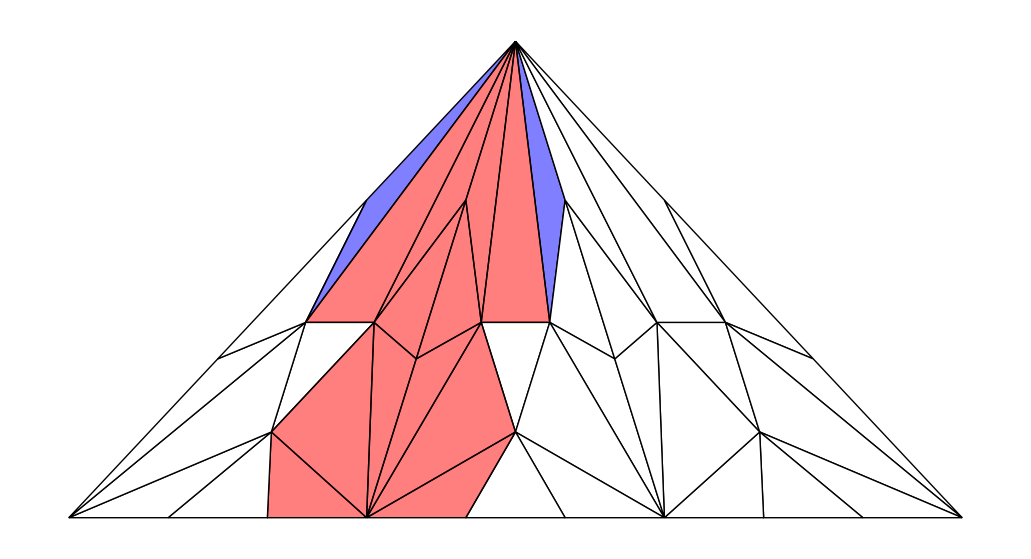
Figure 5. Opposite cliques in $Input(\{v_{0}\},0)$ of a 3-process task

Opposite cliques in $Input(\{v_{0}\},0)$ of a 3-process task

For each pair $(U,V)$, the input complex $Input(U,V)$ can be seen as the joining of a $|U|$-simplex $s^{top}$ and the chromatic subdivision of a $|\Pi-U|$-simplex. $Input(U,V)$ can be further divided into a set of input complexes, each of which corresponds to a subset of $(\Pi-U)$. Suppose that there exists a protocol for each such input complex. To distinguish these protocols, we assign a different label $[(U,V),(U^{{}^{\prime}},V^{{}^{\prime}})]$ to each protocol, where $U^{{}^{\prime}}$ is a subset of the process set $(\Pi-U)$ and is the first process set to execute. In other words, the label is now a list of pairs $(U,V)$.

Let $s^{n}$ be an n-simplex reached from the join of $s^{top}$ and a $|\Pi-U|$-simplex $C_{1}$ by the schedule $\alpha$. We define the opposite clique of $s^{n}$ as an n-simplex reached by $\alpha$ from the join of $s^{top}$ and $C_{2}$ where $C_{2}$ is calculated from $C_{1}$. An n-clique whose intersection simplex is in $s^{top}$ may have an opposite clique with a larger carrier, as the example shows. Note that using the techniques in the proof of Lemma 5.7, other n-cliques will not have this issue. We introduce a rule, which is referred to as the carrier rule in subsequent discussions. Let $\sigma$ be an n-clique in $Ch^{r_{max}-1}(Input(U,V))$. The vertices in $\sigma$ can be divided into two types: intersection vertices and internal vertices. The intersection simplex consisting of intersection vertices is in $s^{top}$. If some subsimplex $\tau$ of $\sigma$ has a smaller carrier in the opposite clique, then it is not safe to use the values of the opposite clique to terminate the vertices in the subdivision of $\tau$. Instead, the vertices in the subdivision of $\tau$ will terminate with the value of some intersection vertex. The intersection vertex is chosen to be the projection of $\tau$ to the intersection simplex. There will be no violation of the task specification, since the intersection vertices have only seen the input values of the processes in $U$, which all the vertices in $Input(U,V)$ have seen, and the task is assumed to be colorless. We have to show that the carrier rule will not cause any conflict of values. Recall that the opposite cliques of two n-cliques sharing some vertex will share the vertex with the same process id. If some other n-clique $\sigma^{{}^{\prime}}$ contains a vertex $v$ terminated by the carrier rule, then by the property of opposite cliques, the vertex $v$ will also have a larger carrier in the opposite clique of $\sigma^{{}^{\prime}}$. This means that $v$ will terminate with the carrier rule, and the terminated value will be identical since the projection to $s^{top}$ will be the same vertex.

So what is the difference of phase 1 when the restricted protocol for $Input(U,V)$ is replaced by a sequence of restricted protocols for $Input((U,V),(U^{{}^{\prime}},V^{{}^{\prime}}))$? We have to check whether the previous results can still be used. First, we will show that Lemma 5.7 can be used for these subprotocols: if an n-clique $\sigma$ has an intersection with the input complex with some label $[(U,V),(U^{{}^{\prime}},V^{{}^{\prime}})]$, then there exists an opposite clique of $\sigma$ with this label. Suppose that an n-clique $\sigma$ has some intersection vertices with $Input((U,V),(U^{{}^{\prime}},V^{{}^{\prime}}))$. We will use its opposite clique $\sigma^{{}^{\prime}}$ with the label $(U,V)$ to construct its opposite clique with the label $(U,V),(U^{{}^{\prime}},V^{{}^{\prime}})$. If $\sigma^{{}^{\prime}}$ is in $Input((U,V),(U^{{}^{\prime}},V^{{}^{\prime}}))$, then $\sigma^{{}^{\prime}}$ is the opposite clique of $\sigma$ with the label $[(U,V),(U^{{}^{\prime}},V^{{}^{\prime}})]$. Otherwise, $\sigma^{{}^{\prime}}$ is in another input complex $Input((U,V),(U^{{}^{\prime\prime}},V^{{}^{\prime\prime}}))$. Let $V_{int}$ be the set of vertices shared by $\sigma$ and $Input((U,V),(U^{{}^{\prime}},V^{{}^{\prime}}))$. Then $\sigma^{{}^{\prime}}$ will also contain $V_{int}$. Therefore, there exists an opposite clique of $\sigma^{{}^{\prime}}$ with the label $[(U,V),(U^{{}^{\prime}},V^{{}^{\prime}})]$. We will use the opposite clique of $\sigma^{{}^{\prime}}$ as the opposite clique of $\sigma$.

Next, we prove that there will be no conflict of output values. If the vertex $v$ is shared by two n-cliques having an intersection with $Input((U,V),(U^{{}^{\prime}},V^{{}^{\prime}}))$, then the opposite cliques with $(U,V)$ will share the vertex with the same process id. When the opposite cliques with the label $(U,V)$ are both in or not in $Input([(U,V),(U^{{}^{\prime}},V^{{}^{\prime}}))$, the opposite cliques with the label $[(U,V),(U^{{}^{\prime}},V^{{}^{\prime}})]$ will share the vertex with the same process id. If only one of the opposite cliques with label $(U,V)$ denoted by $s^{oc}$ is in $Input([(U,V),(U^{{}^{\prime}},V^{{}^{\prime}}))$, then the vertex $v$ will be at the intersection of two input complexes. The opposite clique of $s^{oc}$ with the label $[(U,V),(U^{{}^{\prime}},V^{{}^{\prime}})]$ will not change the intersection vertices, including the vertex $v$. Therefore, the opposite cliques with the label $[(U,V),(U^{{}^{\prime}},V^{{}^{\prime}})]$ will still share the vertex with the same process id. Therefore, the input complex $Input(U,V)$ will be replaced by a sequence of input complexes $Input((U,V),(U^{{}^{\prime}},V^{{}^{\prime}}))$ while our interaction framework is kept valid.

After the second phase, the first two process set are determined, which means that the adversary can limit its view to the subcomplex of $S^{t}$ reached from the input complex labeled by $[(U,V),(U^{{}^{\prime}},V^{{}^{\prime}})]$. The adversary can use the techniques in Section 5.2 to generate a protocol for $Input((U,V),(U^{{}^{\prime}},V^{{}^{\prime}}))$. The condition required for connecting output configurations of different labels is that each intersection simplex must be compatible. The carrier rule will not affect these procedures since the carrier rule will change the values of non-intersection vertices. Only the output values of the intersection vertices are used to add layers to the terminated sets.

Theorem 5.18.

For a general colorless task$(\mathcal{I},\mathcal{O},\Delta)$, there exists an adversary that can finalize after the second phase and win against any restricted extension-based prover if and only if there exists a protocol for each $Input((U,V),(U^{{}^{\prime}},V^{{}^{\prime}}))$ and all intersection simplices in the standard chromatic subdivision of all initial configurations are compatible.

By Theorem 5.2, there exists a protocol for $Input(U,V)$ if and only if there exists $\mathcal{O}_{\tau}^{i}$ for some $0\leq i\leq m$, such that the task $(lk(\tau,\mathcal{I})$, $\mathcal{O}_{\tau}^{i}\backslash\tau$, $\Delta_{\tau})$ has a protocol where $\tau$ is $s^{top}$ of $Input(U,V)$. This task is a $|\Pi-U|$-processes task. Let $\rho$ denote $s^{top}$ of $Input((U,V),\allowbreak(U^{{}^{\prime}},V^{{}^{\prime}}))$. Then there exists a protocol for $Input((U,V),\allowbreak(U^{{}^{\prime}},V^{{}^{\prime}}))$ if and only if there exists $(\mathcal{O}_{\tau}^{i})_{\rho-\tau}^{j}$ for some $0\leq i\leq m$ and some $0\leq j\leq m^{{}^{\prime}}$, such that the task $(lk(\rho,\mathcal{I})$, $(\mathcal{O}_{\tau}^{i})_{\rho-\tau}^{j}\backslash(\rho-\tau)$, $\Delta_{\rho})$ has a protocol. The choice of $i$ and $j$ can be arbitrary when we discuss the existence of some $Protocol((U,V),(U^{{}^{\prime}},V^{{}^{\prime}}))$. But if we are talking about extension-based proofs, the choice of $i$ will be unique, since the simplex $s^{top}$ of $Input(U,V)$ is compatible. This consequence can be obtained from the proof of Lemma 5.1.

The decomposition of the protocol for $Input((U,V),(U^{{}^{\prime}},V^{{}^{\prime}}))$ can continue. Suppose that some input complex is labeled by $[(U_{1},V_{1}),\allowbreak...(U_{k},V_{k})]$ where the process set $U_{i}\subseteq\Pi-\sum_{1}^{i-1}U_{l}$ for each $i$, and all properties described above are satisfied. For each pair sequence, the input complex $Input((U_{1},V_{1}),(U_{2},V_{2})\allowbreak...(U_{k},V_{k}))$ can be seen as the join of a $|\sum_{1}^{k}U_{i}|$-simplex $s^{top}$ and the chromatic subdivision of a $|\Pi-\sum_{1}^{k}U_{i}|$-simplex. It will be further divided into a sequence of input complexes, each of which corresponds to a subset of the process set $\Pi-\sum_{1}^{k}U_{i}$. Suppose that there exists a protocol for each such input complex. To distinguish these protocols, we will assign a different label $[(U_{1},V_{1}),\allowbreak...(U_{k},V_{k}),(U_{k+1},V_{k+1})]$ to each protocol where $U_{k+1}$ is a subset of the process set $(\Pi-\sum_{1}^{k}U_{i})$ and is the first process set in the subsequent execution. For convenience, we will denote the old and new labels as $l_{o}$ and $l_{n}$. We will still define the opposite clique of the join of $s^{top}$ and a $|\Pi-\sum_{1}^{k}U_{i}|$-simplex $s^{bot}$ as the join of $s^{top}$ and the opposite clique of $s^{bot}$ in the chromatic subdivision of $|\Pi-\sum_{1}^{k}U_{i}|$-simplex. The carrier rule will be used to avoid violating the task specification.

Lemma 5.7 can be used for the new input complexes: if an n-clique $\sigma$ has an intersection with the protocol for some label $l_{n}$, then there exists an opposite clique of this n-clique with this label. Suppose that an n-clique $\sigma$ has some intersection vertices with some protocol with the label $l_{n}$, denoted by $V_{int}$. By the induction hypothesis, it will have an opposite clique with the label $l_{o}$. If the opposite clique with the label $l_{o}$ of $\sigma$ is in the input complex for the label $l_{n}$, then we will use it as the opposite clique of $\sigma$ with the label $l_{n}$. Otherwise the opposite clique $\sigma^{{}^{\prime}}$ with the label $l_{o}$ is in another input complex, then $\sigma^{{}^{\prime}}$ will also contain the vertices set $V_{int}$. So, there exists an opposite clique of $\sigma^{{}^{\prime}}$ with the label $l_{n}$. We will use the opposite clique of $\sigma^{{}^{\prime}}$ with the label $l_{n}$ as the opposite clique of $\sigma$ with the label $l_{n}$. There will be no conflict of output values. If the vertex $v$ is shared by two n-cliques having an intersection with $Input(l_{n})$, then the opposite cliques with the label $l_{o}$ will share the vertex with the same process id. If the opposite cliques with the label $(U,V)$ are both in or not in $Input(l_{n})$, the opposite cliques with the label $l_{n}$ will share the vertex with the same process id. If only one of the opposite cliques with the label $l_{o}$ denoted by $s^{oc}$ is in $Input(s_{n})$, then the vertex $v$ will be at the intersection of two subprotocols. The opposite clique of $s^{oc}$ with the label $l_{n}$ will not change the intersection vertices, including the vertex $v$. Therefore, the opposite cliques with the label $l_{o}$ will still share the vertex with the same process id.

After phase $k$, the first $k$ process sets are determined which means the adversary can limit itself to the subcomplex of $S^{t}$ reached from the input complex labeled with $[(U_{1},V_{1}),(U_{2},V_{2})\allowbreak...(U_{k},V_{k})]$. The adversary can use the techniques in Section 5.2 to generate a restricted protocol.

Theorem 5.19.

For a general colorless task $(\mathcal{I},\mathcal{O},\Delta)$, there exists an adversary that can finalize after the $k$-th phase and win against any restricted extension-based prover if and only if there exists a protocol for each $Input((U_{1},V_{1}),(U_{2},V_{2})\allowbreak...(U_{k},V_{k}))$ where $\sum_{1}^{k}U_{i}\subseteq\Pi$ and all intersection simplices in the standard chromatic subdivision of all initial configurations are compatible.

Now we will discuss the case of $\sum_{1}^{k}U_{i}=\Pi$. We will show that any further division of the protocol will be unnecessary. Any further division will still imply the existence of a protocol for $Input([(U_{1},V_{1}),\allowbreak...(U_{k},V_{k})])$ since there must be a protocol for the configurations reached from the schedule which repeats the first partition $U_{1},U_{2},\allowbreak...U_{k}$ of $\Pi$. For example, if the input complex $Input([(U_{1},V_{1}),\allowbreak...(U_{k},V_{k})])$ is further divided into a sequence of input complexes $Input([(U_{1},V_{1}),\allowbreak...(U_{k},V_{k}),\allowbreak(U_{k+1},V_{k+1})])$ where $U_{k+1}$ is a subset of $\Pi$ and there exists a protocol for each such input complex, then there is a protocol for the configurations reached from the schedule which repeats the first partition twice. This protocol can be used as a protocol for $Input([(U_{1},V_{1}),\allowbreak...(U_{k},V_{k})])$ without violating the carrier map. Note that this is not necessarily true for those input complexes labeled by $[(U_{1},V_{1}),\allowbreak...(U_{k},V_{k})]$ such that $\sum_{1}^{k}U_{i}\subsetneqq\Pi$. But this is not the reason why we will not further subdivide the protocol since the existence of a protocol for $Input([(U_{1},V_{1}),\allowbreak...(U_{k},V_{k})])$ is not enough for our requirements: the intersection simplices have to be compatible. If we just use the protocol for $Input([(U_{1},V_{1}),\allowbreak...(U_{k},V_{k})])$, the output configurations of some shared simplices will change, just as the reason why we will not use the standard form of restricted protocols.

Suppose that there is a set of subprotocols for some covering of $Input([(U_{1},V_{1}),\allowbreak...(U_{k},V_{k})])$ where $\sum_{1}^{k}U_{i}=\Pi$. What we will do is to construct a valid protocol for $Input([(U_{1},V_{1}),\allowbreak...(U_{k},V_{k})])$ from these subprotocols. A key observation is that for any intersection simplex of $Input([(U_{1},V_{1}),\allowbreak...(U_{k},V_{k})])$ with other $Input([(U_{1}^{{}^{\prime}},V_{1}^{{}^{\prime}}),\allowbreak...(U_{k}^{{}^{\prime}},\allowbreak V_{k}^{{}^{\prime}})])$ where $\sum_{1}^{k}U_{i}^{{}^{\prime}}=\Pi$, it is assumed to be compatible, and the most central simplex reached from it is contained in only one subprotocol. This means that if we can connect these subprotocols, i.e., have the intersection parts of different subprotocols terminated with the same output configuration, we can generate a protocol that satisfies the requirements of Theorem 5.19. We cannot do the same thing to $Input([(U_{1},V_{1}),\allowbreak...(U_{k},V_{k})])$ where $\sum_{1}^{k}U_{i}\subsetneqq\Pi$ since its intersection simplex with any other input complex which is assumed to be compatible can be shared by more than one subprotocol.

All processes must have seen the input values of the processes in $U_{1}$. Therefore, we can use the most central simplex $s_{c}$ in the subdivision of the simplex corresponding to the set of processes $U_{1}$ to connect the subprotocols. For each intersection simplex $s_{i}$, it corresponds to a process set $U_{k+1}$. We will construct a new subprotocol for $Input([(U_{1},V_{1}),\allowbreak...(U_{k},V_{k}),\allowbreak(U_{k+1},V_{k+1})])$ while keeping the output configuration of $s_{i}$ unchanged. There is a path from some vertex $v_{i}$ of the output configuration of $s_{i}$ to some vertex $v_{c}$ of the output configuration of $s_{c}$ using the original set of subprotocols. First, we will terminate the intersection simplex $s_{i}$ with its output configuration. Then we will terminate each vertex adjacent to the terminated vertices with the value $v_{i}$. Finally, we will add layers corresponding to the path from $v_{i}$ to $v_{c}$. The constructed protocol is valid for $Input([(U_{1},V_{1})\allowbreak...(U_{k+1},V_{k+1})])$ and the terminated values of intersection simplices with other subprotocols will all be $v_{c}$. There always exists a path from $v_{i}$ to $v_{c}$ in which the carrier of each vertex grows smaller since all common simplices between the original subprotocols are compatible. And the carrier of $s_{i}$ is the smallest compared to any other vertex in $Input([(U_{1},V_{1}),\allowbreak...(U_{k},V_{k}),\allowbreak(U_{k+1},V_{k+1})])$. Therefore, using this path can avoid any task specification violation. Most importantly, the terminated values of $s_{i}$ are not changed. We can choose the same $v_{c}$ and build the protocol of $Input([(U_{1},V_{1}),\allowbreak...(U_{k},V_{k}),(U_{k+1},V_{k+1})])$ for each process set $U_{k+1}$. These subprotocols can be united into a valid protocol for $Input([(U_{1},V_{1}),\allowbreak...(U_{k},V_{k})])$. Therefore, we have shown that it is not necessary to further divide the input complex $Input([(U_{1},V_{1}),\allowbreak...(U_{k},V_{k})])$.

Before giving the final result, we want to explain why the finalization after the input complex is restricted to $Input((U_{1},V_{1}),\allowbreak...(U_{k},V_{k}))$ where $\sum_{1}^{k}U_{i}=\Pi$ is sufficient for the adversary to win against any extension-based prover. The prover cannot find a safety violation. To win against the adversary, the only possible way is to construct infinite phases. We assume $U_{i}\subseteq\Pi-\sum_{1}^{i-1}U_{l}$ for each $i$, but what if the adversary chooses to terminate the phases, e.g., by having $U_{2}=U_{1}$? Suppose that the prover ends the phase $i$ by extending the schedule by a process set $U_{i}$, where $\sum U_{i}\subsetneqq\Pi$. By Lemma 5.12, the processes in $\sum U_{i}$ will terminate with some output values after some phase $k_{s}$. So $U_{k_{s}+1}$ contains some process in $\Pi-\sum U_{i}$. In other words, there exists some phase $k_{e}$ where $\alpha(k_{e})$ contains each process in $\Pi$. The restricted input complex after phase $k_{e}$ is therefore contained in some $Input((U_{1},V_{1}),\allowbreak...(U_{k},V_{k}))$ where $\sum_{1}^{k}U_{i}=\Pi$. The adversary can finalize after phase $k_{e}$ and win.

Theorem 5.20.

For a general colorless task$(\mathcal{I},\mathcal{O},\Delta)$, there exists an adversary that can win against any restricted extension-based prover if and only if there exists a protocol for each $Input((U_{1},V_{1}),\allowbreak...(U_{k},V_{k}))$ where $\sum_{1}^{k}U_{i}=\Pi$ and all intersection simplices in the standard chromatic subdivision of all initial configurations are compatible.

6. Reductions of colorless tasks

In this section, we will present an application of our results in Section 5. We can use Theorem 5.20 to discuss the reductions of colorless tasks in a totally topological way. If a colorless task $\mathcal{T}=(\mathcal{I},\mathcal{O},\Delta)$ reduces to another colorless task $\mathcal{S}=(\mathcal{I}^{{}^{\prime}},\mathcal{O}^{{}^{\prime}},\Delta^{{}^{\prime}})$, then there exists a composition of protocols $(\mathcal{P}_{2l},\mathcal{P}_{2l+1},\Xi_{2l+1})*\cdots*(\mathcal{P}_{0},\mathcal{P}_{1},\Xi_{1})$ that can solve the task $\mathcal{T}$. Each protocol $(\mathcal{P}_{i-1},\mathcal{P}_{i},\Xi_{i})$, $1\leq i\leq 2l+1$ is an immediate snapshot protocol or a protocol that solves the task $\mathcal{S}$. So we will use the notation in Section 4 and denote the composed protocols as $(B_{l+1}\cdot A_{l}\cdot B_{l}\cdot A_{l-1}\cdots A_{1}\cdot B_{1})$ where each $A_{i}$ is the same protocol $A$ solving task $\mathcal{S}$ and each $B_{i}$ is an IIS protocol. If task $\mathcal{S}$ has no extension-based proofs, by Theorem 5.20 there exists a restricted protocol for each $Input((U_{1},V_{1}),\allowbreak...(U_{k},V_{k}))$ where $\sum_{1}^{k}U_{i}=\Pi$ and all intersection simplices in the standard chromatic subdivision of all initial configurations are compatible. In other words, $A_{i}$ is not a valid protocol, but a sequence of subprotocols for each $Input((U_{1},V_{1}),\allowbreak...(U_{k},V_{k}))$. However, we will still use the notation of the composed protocol and construct a protocol for each such input complex of the task $\mathcal{T}$ from these subprotocols of $\mathcal{S}$.

For each input configuration of $\mathcal{T}$ denoted by $C$, our goal is to construct a sequence of subprotocols from each input complex $Input((U_{1},V_{1}),\allowbreak...(U_{k},V_{k}))$ in $\mathcal{I}$ to the output complex of task $\mathcal{T}$. And these subprotocols shall satisfy the compatibility condition. This is achieved by induction: for each $Input((U_{1},V_{1}),\allowbreak...(U_{k},V_{k}))$ we will subdivide $Input((U_{1},V_{1}),\allowbreak...(U_{k},V_{k}))$ and build a protocol from each simplex of the subdivision to the output complex of some protocol in the sequence. Each of such protocols is labeled with $[(U_{1},V_{1}),\allowbreak...(U_{k},V_{k})]$. The first requirement is about protocols with different labels. For each intersection simplex of the two input complexes with labels $b_{1}$ and $b_{2}$, protocols with labels $b_{1}$ and $b_{2}$ containing the most central simplex will terminate it with the same output configuration. Let $s_{c}$ denote the subsimplex of $Input((U_{1},V_{1}),\allowbreak...(U_{k},V_{k}))$ corresponding to $U_{1}$. The second requirement is that the most central simplex of each intersection simplex should be connected to the most central simplex of $s_{c}$ by a path in which the carrier of each vertex becomes smaller. If the path goes through two protocols with the same label, it will have a vertex in some shared output configuration of two protocols.

First, we will construct a protocol from each input complex $Input((U_{1},V_{1}),\allowbreak...(U_{k},V_{k}))$ to the output complex of $B_{1}$ by limiting the protocol $B_{1}$ to each input complex. No subdivision of any $Input((U_{1},V_{1}),\allowbreak...(U_{k},V_{k}))$ is needed here, and therefore the second requirement is satisfied. Since all these protocols are obtained from the same protocol $B_{1}$, any intersection simplex will be mapped to the same complex in the output complex of $B_{1}$, and therefore is compatible.

The induction procedures will be different depending on the next protocol. By the induction hypothesis, for each $Input((U_{1},\allowbreak V_{1}),\allowbreak...(U_{k},V_{k}))$, we have constructed a protocol from each simplex $\sigma$ in the $n$-th iterated chromatic subdivision to the output complex of the previous protocol. By the asynchronous computability theorem, we know that there exists a color-preserving simplicial map from the $m$-th iterated standard chromatic subdivision of $\sigma$ to the output complex of the last protocol. We will choose $m$ to be the largest of any $\sigma$.

If the next protocol is some $B_{i}$ which is some IIS protocol. For each $Input((U_{1},V_{1}),\allowbreak...(U_{k},V_{k}))$, we will define a set of protocols to the output complex of $B_{i}$ by composing the already constructed protocols with $B_{i}$. Two requirements are satisfied since they are satisfied when using the old set of protocols.

Otherwise the next protocol is some protocol $A_{i}$ which is in fact a sequence of subprotocols of the task $\mathcal{S}$. For each simplex in the $n$-th iterated standard chromatic subdivision of $Input((U_{1},V_{1}),\allowbreak...(U_{k},\allowbreak V_{k}))$, the range of a constructed protocol from it to the input complex of $A_{i}$ will be an n-dimensional complex. We cannot compose this protocol with $A_{i}$ to obtain the new protocol as we have done, since $A_{i}$ is not a real protocol at all. So for each $Input((U_{1},V_{1}),\allowbreak...(U_{k},V_{k}))$, we will subdivide it $(n+m+1)$ times. For each simplex $\sigma$ in the $(n+m+1)$-th iterated standard chromatic subdivision, we will define a protocol from $\sigma$ to the input complex of $A_{i}$ by limiting some existing constructed protocol denoted by $P_{c}$ to $\sigma$. Note that if two such protocols are built from the same $P_{c}$, then any intersection simplex between them is compatible. The range of each such protocol from $\sigma$ is in some $Input((U_{1}^{{}^{\prime}},V_{1}^{{}^{\prime}}),\allowbreak...(U_{k}^{{}^{\prime}},V_{k}^{{}^{\prime}}))$ of task $\mathcal{S}$. Then we will compose this protocol with its corresponding subprotocol of the task $\mathcal{S}$ to construct a new protocol from $\sigma$ to the output complex of $A_{i}$. To prove the first requirement, for each intersection simplex, consider the new protocol for the $(n+m+1)$-th iterated standard chromatic subdivision of it. It will be mapped to a complex in the output complex of $A_{i}$ in which the most central facet will be shared by the newly constructed protocols with different labels. Therefore the first requirement is satisfied.

By the induction hypothesis, the most central simplex of each intersection simplex should be connected to the most central simplex of $s_{c}$ by a path $v_{0},v_{1},....v_{l}$ in the $n$-th iterated standard chromatic subdivision in which the carrier of each vertex is growing smaller. We will first link the $v_{0}^{{}^{\prime}}$ of the most central simplex in the $(n+m+1)$-th iterated standard chromatic subdivision to $v_{0}$. Using the same argument in the proof of the first requirement, we know that any intersection simplex between new protocols constructed from the same old protocol $P_{c}$ will be compatible. Therefore the path from $v_{0}^{{}^{\prime}}$ to $v_{0}$ is possible and the vertex on the boundary of two protocols is in the shared output configuration. Readers can imagine a line from $v_{0}^{{}^{\prime}}$ to $v_{0}$. Once it passes some boundary between protocols, it will choose to go through the center of the boundary. The carrier of each vertex in this deviation will be the same. For the same reason, a path can be constructed from $v_{l}$ to $v_{l}^{{}^{\prime}}$. Now suppose that $v_{0},v_{1},...v_{l^{{}^{\prime}}}$ where $l^{{}^{\prime}}<l$ is in the same simplex of the $n$-th iterated standard chromatic subdivision. Again, we are able to construct a carrier-shrinking path from $v_{0}$ to $v_{l^{{}^{\prime}}}$ in which the vertex on the boundary of two protocols is in the shared output configuration. The vertex $v_{l^{{}^{\prime}}}$ is in the shared configuration $\tau$ of protocols for two simplices containing it in $n$-th iterated standard chromatic subdivision, but may not be in the shared configuration now since only some simplex $\tau^{{}^{\prime}}$ reached from $\tau$ is shared now. We can construct a path from $v_{l^{{}^{\prime}}}$ to $\tau^{{}^{\prime}}$ and then to $v_{l^{{}^{\prime}}}$ again. Note that the carrier of each vertex in this path will be the same. Then we will use the same techniques to each set of vertices $v_{l^{{}^{\prime}}},...v_{l^{{}^{\prime\prime}}}$ in the same simplex of the $n$-th iterated standard chromatic subdivision. The vertex $v_{l}$ is finally reached and will join the path from $v_{l}$ to $v_{l}^{{}^{\prime}}$. So we have constructed a carrier-shrinking path from $v_{0}^{{}^{\prime}}$ to $v_{l}^{{}^{\prime}}$ and if it goes through two protocols, some vertex will be in their shared configuration. Induction procedures are proved.

Finally, we will use the carrier-shrinking paths between intersection simplices to construct a subprotocol from each $Input((U_{1},V_{1}),\allowbreak...(U_{k},\allowbreak V_{k}))$ to the output complex of task $\mathcal{T}$. Since we have proved that any division of a protocol for $Input((U_{1},V_{1}),\allowbreak...(U_{k},V_{k}))$ is unnecessary, the techniques in the proof of Theorem 5.20 are used to generate such a subprotocol. The intersection simplices of these subprotocols will be compatible since the second requirement is maintained, and the merged subprotocol will not change the output values of most central simplex of an intersection simplex. Therefore, we have constructed a protocol for each input complex $Input((U_{1},V_{1}),\allowbreak...(U_{k},V_{k}))$ of the task $\mathcal{T}$ and any intersection simplex is compatible. By Theorem 5.20, there is no extension-based proof for the task $\mathcal{T}$. Therefore, we have proved the contrapositive of Theorem 4.1 for general colorless tasks.

7. Conclusions

In this paper, we solve most of the open questions proposed in (BE, 21). We have shown that if there is a reduction using multiple instances of $\mathcal{S}$ from task $\mathcal{T}$ to $\mathcal{S}$ and there is no augmented extension-based proof that no protocol can solve $\mathcal{S}$, then there is no augmented extension-based proof that no protocol can solve $\mathcal{T}$. Although most of the reductions used in research will not use more than one instance, our result makes the choice of reduction easier. A more important contribution is that we prove the topological properties for colorless tasks to have no extension-based proofs. Previous work is related to some specific tasks, such as the $(n,k)$-set agreement task, and this is the first attempt for general tasks. We introduce a more general interaction procedure for the prover and the adversary. We have also shown that assignment queries will not give more power to the prover. Different versions of extension-based proofs are equivalent in power for colorless tasks. Our adversarial strategy does not require the condition that the task is colorless before the finalization part in Section 5.2.4. An open problem that remains is to extend our results to general tasks or to general tasks with the minimum requirements. And we do believe that the concept of opposite cliques can be used in future researches of extension-based proofs and perhaps other questions of distributed computing.