Matrix-Scaled Consensus over Undirected Networks

Abstract

In this paper, we propose matrix-scaled consensus algorithms for linear dynamical agents interacting over an undirected network. These algorithms are designed to make the state vectors of all agents to asymptotically agree up to some matrix scaling weights. First, the matrix scaled Laplacian and its algebraic properties are examined. Second, we propose matrix-scaled consensus algorithms for networks of single integrators with or without constant parametric uncertainties. Third, observer-based matrix-scaled consensus algorithms for homogeneous or heterogeneous linear agents are designed. The effectiveness of the proposed algorithms are asserted by rigorous mathematical analysis and supported by numerical simulations.

I Introduction

Collective behaviors displayed in nature such as bird flocking, fish schooling, synchronous fireflies, have inspired a lot of research works. Though simple, the consensus algorithm has been widely used for modeling and studying such striking phenomena [1]. It is interesting that a lot of multiagent systems such as autonomous vehicle formations, electrical system, sensor networks, or social networks can be coordinated by appropriately applying consensus algorithms and its modifications [2, 3].

Consider a network in which the interactions between subsystems, or agents, is modeled by a graph. In the consensus algorithm, each agent updates its state based on the sum of the relative states with its nearby agents. If the interaction graph is connected, the agents’ states asymptotically converge to a common point in the space, and the system is said to asymptotically achieve a consensus [1].

A (scalar) scaled consensus model was proposed in [4], in which each agent has a nonzero scalar scaling gain and updates its state variable based on the sum of differences in the scaled states. Under the scaled consensus model, the scaled states of all agents agree to the same virtual consensus value, and the state variable of each agent converges to a value differing from the virtual consensus value by an inverse of the scaling gain. Thus, under the scalar scaled consensus algorithm [4], and suppose that each agent has a state vector, the state vectors of all agents asymptotically distributed along a straight line through the origin. The scaled consensus system can describe a cooperative network, where agents have different levels of consensus on a single topic. Further studies of the scalar scaled consensus algorithm with consideration to switching graphs, time delays, disturbance attenuation, or different agents’ models can be found in the literature [5, 6, 7, 8, 9, 10, 11].

This paper proposes a multi-dimensional generalization of the scaled consensus model in [4]. We firstly consider an undirected network of single integrator agents as a basic setup. Each agent has a state vector and a possibly non-symmetric positive or negative definite scaling matrix. The agent updates the state variables based on the relative matrix-scaled state vectors. Several algebraic properties of the matrix scaled Laplacian, which determines the asymptotic behavior of the whole system, are derived. Specifically, it is shown that the matrix-scaled states eventually agree to a virtual consensus vector. The state vector of each agent asymptotically converges to a vector, which can be obtained from the virtual consensus point by a linear transformation determined by the inverse of its scaling matrix. Thus, all agents with the same scaling matrix converge to a common point in the space, and clustering behaviors usually happen. To accommodate more complicated interactions, nonlinear matrix-scaled consensus algorithms and corresponding Lyapunov-based analysis are also provided. It is worth noting that in the proposed matrix-scaled consensus model, the scaling matrices are not limited to rotation matrices such as the algorithms considered in [12, 13, 14, 15, 16]. In [17], the proposed model was interpreted as a multi-dimensional model opinion dynamics, where the positive/negative definite scaling matrix weights capture the private belief system of an individual on $d$ logically dependent topics. Clustering happens as the private belief system of each individual is usually different from each other and not perfectly aligned with a social norm. Second, we study the matrix-scaled consensus algorithm for a system of single integrators with parametric uncertainties. An adaptive scheme is developed, which guarantees the system to eventually achieve matrix-scaled consensus. If in addition, a persistently exciting condition is satisfied, the estimate variables eventually converge to the precise parameters. Third, we consider a network of homogeneous linear agents and propose an observer-based matrix-scaled consensus algorithm. It is shown that the agents asymptotically achieve matrix-scaled consensus with regard to a trajectory of a virtual agent. If we specify the agents to be linear oscillators in 2D, and the scaling matrices to be a composition of rotation and expansion/compression matrices, the asymptotic biases in phase and magnitude of each agent’s trajectory with a common oscillator can be determined by the scaling matrices. Thus, the algorithms can be used for designing robot’s trajectories, referenced voltages in circuits, or explaining the alternation of temperature during four seasons. Lastly, as practical networks often consists of agents with different sizes and capacities, we propose a matrix-scaled consensus algorithm for a network of heterogeneous linear agents. The proposed algorithm combines the corresponding matrix-scaled consensus algorithm for homogeneous linear agents with a disturbance observer which compensates the differences between each agent’s model and a pre-specified one. The main challenges and differences in the analysis of our proposed algorithms with regard to the existing consensus algorithms for general linear agents in the literature, e.g., [18, 19, 20, 21, 22, 23, 24], are originated from the asymmetry of the matrix scaled Laplacian and the multi-dimension of the problem.

The remainder of this paper is organized as follows. Section II provides theoretical background, problem formulation, and several properties of the matrix-scaled Laplacian. Matrix-scaled consensus algorithms for single integrator agents with and without parametric uncertainties are proposed and examined in Section III. Section IV studies matrix-scaled consensus for networks of homogeneous and heterogeneous linear agents. Simulations are given in Section V to support the theoretical results. Finally, Section VI concludes the paper.

II Preliminaries

II-A Notations

In this paper, the sets of real, complex, and natural numbers are denoted by $\mathbb{R},\mathbb{C}$ and $\mathbb{N}$, respectively. Scalars are denoted by lowercase letters, while bold font normal and capital letters are used for vectors and matrices, respectively. We denote $\mathbf{1}_{d}\in\mathbb{R}^{d}$ the $d$-dimensional vector of all 1 an $\mathbf{0}_{m\times n}\in\mathbb{R}^{m\times n}$ the matrix of all zeros. The transpose of a matrix $\mathbf{A}\in\mathbb{R}^{m\times n}$ is denoted by $\mathbf{A}^{\top}$. The kernel, image, rank, and determinant of $\mathbf{A}$ are respectively denoted as ker$(\mathbf{A})$, im$(\mathbf{A})$, rank($\mathbf{A}$), and $\text{det}(\mathbf{A})$. A diagonal matrix with elements $a_{1},a_{2},\ldots,a_{n}$ is denoted by $\text{diag}(a_{1},a_{2},\ldots,a_{n})$. The 2-norm ($\infty$-norm) of a vector $\mathbf{x}=[x_{1},\ldots,x_{d}]^{\top}$ is denoted by $\|\mathbf{x}\|=\sqrt{\sum_{i=1}^{d}x_{i}^{2}}$ (correspondingly, $\|\mathbf{x}\|_{\infty}=\max_{i\in\{1,\ldots,d\}}|x_{i}|$). The 2-norm of a real matrix $\mathbf{A}$, denoted by $\|\mathbf{A}\|$, is defined as $\max_{\|\mathbf{x}\|=1}\|\mathbf{A}\mathbf{x}\|$. A matrix $\mathbf{A}\in\mathbb{R}^{d\times d}$ is positive definite (negative definite) if and only if $\forall\mathbf{x}\in\mathbb{R}^{d}$, $\mathbf{x}\neq\mathbf{0}_{d}$, then $\mathbf{x}^{\top}\mathbf{A}\mathbf{x}>0$ (resp., $\mathbf{x}^{\top}\mathbf{A}\mathbf{x}<0$). For a real, symmetric positive semidefinite matrix $\mathbf{A}\in\mathbb{R}^{d\times d}$, which can be diagonalized as $\mathbf{T}^{-1}\mathbf{A}\mathbf{T}=\text{diag}(\omega_{1},\ldots,\omega_{d})$, we use $\sqrt{\mathbf{A}}$ to denote its square root $\mathbf{T}\text{diag}(\sqrt{\omega_{1}},\ldots,\sqrt{\omega_{d}})\mathbf{T}^{-1}$. Let $\mathbf{x}_{1},\ldots,\mathbf{x}_{n}\in\mathbb{R}^{d}$, the vectorization operator is defined as vec$(\mathbf{x}_{1},\ldots,\mathbf{x}_{n})=[\mathbf{x}_{1}^{\top},\ldots,\mathbf{x}_{n}^{\top}]^{\top}\in\mathbb{R}^{dn}$. Given matrices $\mathbf{A}_{1},\ldots,\mathbf{A}_{n}$, we use blkdiag$(\mathbf{A}_{1},\ldots,\mathbf{A}_{n})$ as the block diagonal matrix with $\mathbf{A}_{k}$, $k=1,\ldots,n$ in the main diagonal.

II-B Graph theory

Consider a undirected graph $\mathcal{G}=(\mathcal{V},\mathcal{E},\mathcal{W})$, where $\mathcal{V}=\{1,\ldots,n\}$ is the set of $n$ vertices, $\mathcal{E}=\{e_{k}=(i,j),~{}k=1,\ldots,m\}\subset\mathcal{V}^{2}$ is the set of $m$ edges, and $\mathcal{W}=\{w_{ij}>0\}_{(i,j)\in\mathcal{E}}$ is the set of positive scalar weights corresponding to each edge of $\mathcal{G}$. By undirectedness, if $(i,j)\in\mathcal{E}$, then $(j,i)\in\mathcal{E}$. Further, it is assumed that there is no self-loop (an edge with the same end vertices $(i,i)$, $i\in\mathcal{V}$) in the graph. The neighbor set of a vertex $i$ is defined as $\mathcal{N}_{i}=\{j\in\mathcal{N}_{i}|~{}(j,i)\in\mathcal{E}\}$. A path is a sequences of vertices connected by edges in $\mathcal{E}$, where each vertex appears one time, except for possibly the starting and the ending vertices. For examples, the path $\mathcal{P}=i_{1}i_{2}\ldots i_{p}$ from $i_{1}$ to $i_{p}$ has $(i_{k},i_{k+1})\in\mathcal{E}$, $k=1,\ldots,p-1$. A cycle is a path with the same starting and ending vertices. A graph is connected if there exists a path between any two vertices in $\mathcal{V}$.

A spanning subgraph $\mathcal{G}^{\prime}=(\mathcal{V}^{\prime},\mathcal{E}^{\prime},\mathcal{W}^{\prime})$ of $\mathcal{G}$ has $\mathcal{V}^{\prime}=\mathcal{V}$ and $\mathcal{E}\subseteq\mathcal{E}^{\prime}$. A spanning tree of $\mathcal{G}$ is a connected spanning sub-graph of $\mathcal{G}$ with $n-1$ edges. Let $\mathcal{T}$ be a spanning tree of $\mathcal{G}$ and consider an arbitrary labeling and orientation of the edges in $\mathcal{E}$ so that $n-1$ edges of $\mathcal{E}(\mathcal{T})$ are $e_{1},\ldots,e_{n-1}$.

Corresponding to this labeling and edge orientation, the incidence matrix of $\mathcal{G}$ is defined as $\mathbf{H}=[h_{ki}]\in\mathbb{R}^{m\times n}$, where $h_{ki}=-1$ if $e_{k}=(i,j)$, $h_{ki}=-1$ if $e_{k}=(i,j)$, $h_{ki}=1$ if $e_{k}=(j,i)$, and $h_{ki}=0$ in other cases. It is wellknown that if $\mathcal{G}$ is a connected graph, we have rank$(\mathbf{H})=n-1$ and $\mathbf{H}\mathbf{1}_{n}=\mathbf{0}_{m}$ [25].

Let $\mathbf{H}_{\mathcal{T}}\in\mathbb{R}^{(n-1)\times n}$, and $\mathbf{H}_{\mathcal{C}}\in\mathbb{R}^{(m-n+1)\times n}$ denote the corresponding incidence matrices of the subgraphs $\mathcal{T}$, and the subgraph $(\mathcal{V},\mathcal{E}\setminus\mathcal{E}(\mathcal{T}),\mathcal{W}\setminus\mathcal{W}(\mathcal{T}))$. Then, we can express the incidence matrix as

$$\mathbf{H}=\begin{bmatrix}\mathbf{H}_{\mathcal{T}}\\ \mathbf{H}_{\mathcal{C}}\end{bmatrix}=\begin{bmatrix}\mathbf{I}_{n-1}\\ \mathbf{T}\end{bmatrix}\mathbf{H}_{\mathcal{T}}=\mathbf{R}\mathbf{H}_{\mathcal{T}},$$

where $\mathbf{H}_{\mathcal{T}}\in\mathbb{R}^{(n-1)\times n}$, $\mathbf{H}_{\mathcal{C}}\in\mathbb{R}^{(m-n+1)\times n}$, and $\mathbf{T}=\mathbf{H}_{\mathcal{C}}\mathbf{H}_{\mathcal{T}}(\mathbf{H}_{\mathcal{T}}\mathbf{H}_{\mathcal{T}}^{\top})^{-1}$ [26]. The graph Laplacian of $\mathcal{G}$ can be defined as $\mathbf{L}=[l_{ij}]=\mathbf{H}^{\top}\mathbf{W}\mathbf{H}\in\mathbb{R}^{n\times n},$ where $\mathbf{W}=\text{diag}(\ldots,w_{ij},\ldots)=\text{diag}(w_{1},\ldots,w_{m})$. The matrix $\mathbf{L}$ of a connected graph is symmetric positive semidefinite, with spectrum $0=\lambda_{1}<\lambda_{2}\leq\ldots\leq\lambda_{n}$, and ker$(\mathbf{L})=\text{im}(\mathbf{1}_{n})$.

II-C Agents’ models and the group’s objective

In this paper, we consider an $n$-agent system interacted via an undirected weighted graph $\mathcal{G}$. The dynamics of each agent is modeled by either

1. single-integrator with parametric uncertainty:

   $$\dot{\mathbf{x}}_{i}=\mathbf{u}_{i}+\bm{\phi}_{i}(t,\mathbf{x}_{i})\bm{\theta}_{i},~{}i=1,\ldots,n,$$ (1)

   where $\mathbf{x}_{i},\mathbf{u}_{i}\in\mathbb{R}^{d}$ are the state variable vector and the control input, $\bm{\phi}_{i}(t,\mathbf{x}_{i}),~{}\dot{\bm{\phi}}_{i}(t,\mathbf{x}_{i})\in\mathbb{R}^{d\times r}$ are the matrices of known bounded continuous functions, and $\bm{\theta}_{i}\in\mathbb{R}^{r}$ is a vector of constant unknown parameters; or

2. homogeneous linear agents

   $$\dot{\mathbf{x}}_{i} =\mathbf{A}\mathbf{x}_{i}+\mathbf{B}\mathbf{u}_{i},$$ (2a)

   $$\mathbf{y}_{i} =\mathbf{C}\mathbf{x}_{i},~{}i=1,\ldots,n,$$ (2b)

   where $(\mathbf{A},\mathbf{B})$ is stabilizable and $(\mathbf{A},\mathbf{C})$ is observable.

3. heterogeneous linear agents

   $$\dot{\mathbf{x}}_{i} =\mathbf{A}_{i}\mathbf{x}_{i}+\mathbf{B}_{i}\mathbf{u}_{i},$$ (3a)

   $$\mathbf{y}_{i} =\mathbf{C}_{i}\mathbf{x}_{i},~{}i=1,\ldots,n,$$ (3b)

   where $(\mathbf{A}_{i},\mathbf{B}_{i})$ is stabilizable and $(\mathbf{A}_{i},\mathbf{C}_{i})$ is observable, $\forall i\in\{1,\ldots,n\}$.

We associate to each agent a scaling matrix $\mathbf{S}_{i}\in\mathbb{R}^{d\times d}$ ($d\geq 2$) and a state vector $\mathbf{x}_{i}\in\mathbb{R}^{d}$. The matrix $\mathbf{S}_{i}$ is either positive definite or negative definite. For each scaling matrix, we define a matrix signum function

$$\text{sign}(\mathbf{S}_{i})=\left\{{\begin{array}[]{*{20}{ll}}{1},&\text{if $\mathbf{S}_{i}$ is positive definite},\\ {-1},&\text{if $\mathbf{S}_{i}$ is negative definite}.\end{array}}\right.$$ (6)

and an absolute matrix function $|\mathbf{S}_{i}|=\text{sign}(\mathbf{S}_{i})\mathbf{S}_{i}$. It is not hard to see that $\text{sign}(\mathbf{S}_{i})=\text{sign}(\mathbf{S}_{i}^{\top})=\text{sign}(\mathbf{S}_{i}^{-1})$, and $|\mathbf{S}_{i}^{-1}|=|\mathbf{S}_{i}|^{-1}$. Let $\mathbf{x}=\text{vec}(\mathbf{x}_{1},\ldots,\mathbf{x}_{n})$, $\mathbf{S}=\text{blkdiag}(\mathbf{S}_{1},\ldots,\mathbf{S}_{n})$, and $|\mathbf{S}|=\text{blkdiag}(|\mathbf{S}_{1}|,\ldots,|\mathbf{S}_{n}|)$, we aim to design matrix-scaled consensus algorithms so that $\mathbf{x}(t)\to\mathcal{C}_{S}$ as $t\to+\infty$, $\forall\mathbf{x}(0)$, where

$$\mathcal{C}_{S}=\{\mathbf{x}\in\mathbb{R}^{dn}|~{}\mathbf{S}_{i}\mathbf{x}_{i}=\mathbf{S}_{j}\mathbf{x}_{j},~{}\forall i,j=1,\ldots,n\}.$$ (7)

is the matrix-scaled consensus (MSC) set.

The following lemma will be used throughout this paper.

Lemma II.1

The matrix $\bm{\Omega}=(\text{sign}(\mathbf{S})\mathbf{L}\otimes\mathbf{I}_{d})\mathbf{S}$ has $d$ zero eigenvalues and $dn-d$ eigenvalues with positive real parts. The left and right kernels of $\bm{\Omega}$ are spanned by columns of $(\text{sign}(\mathbf{S})\mathbf{1}_{n})\otimes\mathbf{I}_{d}$ and $\mathbf{S}^{-1}(\mathbf{1}_{n}\otimes\mathbf{I}_{d})$, respectively.

Proof:

Since two matrices $\mathbf{M}=\mathbf{S}\bm{\Omega}\mathbf{S}^{-1}=|\mathbf{S}|(\mathbf{L}\otimes\mathbf{I}_{d})$ and $\bm{\Omega}$ are similar, they have the same spectrum. Because $|\mathbf{S}|$ is positive definite, rank$(\mathbf{M})=\text{rank}(\mathbf{L}\otimes\mathbf{I}_{d})=dn-d$, and thus $\mathbf{M}$ has $d$ zero eigenvalues. Next, let $\bar{\mathbf{H}}=\mathbf{H}\otimes\mathbf{I}_{d}$, $\bar{\mathbf{W}}=\mathbf{W}\otimes\mathbf{I}_{d}$, $\bar{\mathbf{L}}=\mathbf{L}\otimes\mathbf{I}_{d}$,

$$\mathbf{X}=\begin{bmatrix}\mathbf{I}_{dn}&s^{-1}\mathbf{|S|}\bar{\mathbf{H}}^{\top}\sqrt{\overline{\mathbf{W}}}\\ \sqrt{\overline{\mathbf{W}}}\bar{\mathbf{H}}&\mathbf{I}_{dm}\end{bmatrix},~{}\mathbf{Y}=\begin{bmatrix}\mathbf{I}_{dn}&\mathbf{0}_{dn\times dm}\\ -\sqrt{\overline{\mathbf{W}}}\bar{\mathbf{H}}&\mathbf{I}_{dm}\end{bmatrix},$$

for any $0\neq s\in\mathbb{C}$, we have

$$\mathbf{X}\mathbf{Y} =\begin{bmatrix}\mathbf{I}_{dn}-s^{-1}\mathbf{|S|}\bar{\mathbf{L}}&s^{-1}\mathbf{|S|}\bar{\mathbf{H}}^{\top}\sqrt{\overline{\mathbf{W}}}\\ \mathbf{0}_{dm\times dn}&\mathbf{I}_{dm}\end{bmatrix},$$

$$\mathbf{Y}\mathbf{X} =\begin{bmatrix}\mathbf{I}_{dn}&s^{-1}\mathbf{|S|}\bar{\mathbf{H}}^{\top}\sqrt{\overline{\mathbf{W}}}\\ \mathbf{0}_{dm\times dn}&\mathbf{I}_{dm}-s^{-1}\sqrt{\overline{\mathbf{W}}}\bar{\mathbf{H}}\mathbf{|S|}\bar{\mathbf{H}}^{\top}\sqrt{\overline{\mathbf{W}}}\end{bmatrix}.$$

From the fact that $\text{det}(\mathbf{X}\mathbf{Y})=\text{det}(\mathbf{Y}\mathbf{X})$, one has

$$\text{det}(\mathbf{I}_{dn}-s^{-1}\mathbf{|S|}\bar{\mathbf{L}})=\text{det}(\mathbf{I}_{dm}-s^{-1}\sqrt{\overline{\mathbf{W}}}\bar{\mathbf{H}}\mathbf{|S|}\bar{\mathbf{H}}^{\top}\sqrt{\overline{\mathbf{W}}}),$$

$$s^{d(m-n)}\text{det}(s\mathbf{I}_{dn}-\mathbf{|S|}\bar{\mathbf{L}})=\text{det}(s\mathbf{I}_{dm}-\sqrt{\overline{\mathbf{W}}}\bar{\mathbf{H}}\mathbf{|S|}\bar{\mathbf{H}}^{\top}\sqrt{\overline{\mathbf{W}}}).$$

Thus, the nonzero eigenvalues of two matrices $\mathbf{M}=\mathbf{|S|}\bar{\mathbf{L}}$ and $\mathbf{N}=\sqrt{\overline{\mathbf{W}}}\bar{\mathbf{H}}\mathbf{|S|}\bar{\mathbf{H}}^{\top}\sqrt{\overline{\mathbf{W}}}$ are the same. Since $\mathbf{|S|}$ and $\sqrt{\overline{\mathbf{W}}}$ are positive definite, $\forall\mathbf{y}\in\mathbb{R}^{dm}$, $\mathbf{y}^{\top}\mathbf{N}\mathbf{y}=\frac{1}{2}\mathbf{y}^{\top}(\mathbf{N}+\mathbf{N}^{\top})\mathbf{y}=\frac{1}{2}\mathbf{y}^{\top}\sqrt{\overline{\mathbf{W}}}\bar{\mathbf{H}}(\mathbf{|S|}+\mathbf{|S|}^{\top})\bar{\mathbf{H}}^{\top}\sqrt{\overline{\mathbf{W}}}\mathbf{y}\geq 0$. Therefore, $\mathbf{N}$, and thus $\bm{\Omega}$, have $dn-d$ eigenvalues with positive real parts. Finally, the claim on ker$(\bm{\Omega})$ follows by direct computation. ∎

Remark II.1

We will refer to $\bm{\Omega}$ as the matrix-scaled Laplacian since its structure resembles a Laplacian with block matrix weights [27]. If we further assume that $\mathbf{S}_{i}=\mathbf{S}_{i}^{\top},~{}\forall i=1,\ldots,n$, based on [28][Thm. 3], all eigenvalues $\Lambda_{1},\ldots,\Lambda_{dn}$ of $\bm{\Omega}$ are real and

$$\begin{split}\Lambda_{1}&=\ldots=\Lambda_{d}=0,\\ \Lambda_{k}&=\theta_{k}\lambda_{\lceil k/d\rceil},~{}k=d+1,\ldots,dn,\end{split}$$ (8)

where $\lceil x\rceil$ denotes the closest natural number that is greater than or equal to $x$, $\lambda_{k}$ is the $k$-smallest eigenvalue of $\mathbf{L}$ and $\theta_{k}\in[p_{\min},p_{\max}]$, $p_{\min}$ and $p_{\max}$ are respectively the smallest and the largest eigenvalue of all $|\mathbf{S}_{i}|$.

For example, consider $\mathcal{G}=\mathcal{C}_{6}$ - the cycle of length six, and $\mathbf{S}_{i}$ are given as $\mathbf{S}_{1}=\mathbf{S}_{2}=\begin{bmatrix}2&-\frac{\sqrt{3}}{4}\\ -\frac{\sqrt{3}}{4}&\frac{7}{4}\end{bmatrix},~{}\mathbf{S}_{3}=\mathbf{S}_{4}=\begin{bmatrix}2&0\\ 0&1\end{bmatrix},~{}\mathbf{S}_{5}=\mathbf{S}_{6}=\begin{bmatrix}-3&0\\ 0&-1\end{bmatrix}.$ Then, $0=\lambda_{1}<\lambda_{2}=\lambda_{3}=1<\lambda_{4}=\lambda_{5}=3<\lambda_{6}=4$, $p_{\min}=0.5$, $p_{\max}=3$, and the eigenvalues of $\bm{\Omega}$ are $\{0,~{}0,~{}1.059,~{}1.264,~{}2.088,2.387,3.406,3.477,~{}5.051,~{}6.657,$ $~{}7.388,~{}10.222\}$, which all belong to the interval $[0.5,~{}12]$.

III Matrix-scaled consensus algorithms for a network of single-integrator agents

III-A Matrix-scaled consensus of single-integrators

We firstly consider the ideal case, where agents are modeled by single integrators. The matrix-scaled consensus algorithm is proposed as follows

$$\dot{\mathbf{x}}_{i} =\mathbf{u}_{i}=-\text{sign}(\mathbf{S}_{i})\sum_{j\in\mathcal{N}_{i}}(\mathbf{S}_{i}\mathbf{x}_{i}-\mathbf{S}_{j}\mathbf{x}_{j}),\,i=1,\ldots,n.$$ (9)

The asymptotic behavior of the system (9) is summarized in the following theorem.

Theorem III.1

Let the graph $\mathcal{G}$ be connected. Under the algorithm (9), $\mathbf{x}(t)$ exponentially converges to a point in $\mathcal{C}_{S}$.

Proof:

The system can be expressed in the matrix form as follows:

$$\dot{\mathbf{x}}=-(\text{sign}(\mathbf{S})\mathbf{L}\otimes\mathbf{I}_{d})\mathbf{S}\mathbf{x}=-\bm{\Omega}\mathbf{x}.$$ (10)

Let $\mathbf{V}=[\mathbf{v}_{1},\ldots,\mathbf{v}_{dn}]$ and $\mathbf{V}^{-1}=\mathbf{Z}^{\top}$ be orthogonal matrices (which can be chosen with real entries) such that $\mathbf{V}_{[1:d]}=\mathbf{S}^{-1}(\mathbf{1}_{n}\otimes\mathbf{P})$, $\mathbf{Z}_{[1:d]}=(\text{sign}(\mathbf{S})\mathbf{1}_{n}\otimes\mathbf{I}_{d})$, where $\mathbf{P}\in\mathbb{R}^{d\times d}$ has yet to be determined. Since $\mathbf{V}^{-1}\mathbf{V}=\mathbf{I}_{dn}$, we have $(\mathbf{1}_{n}^{\top}\text{sign}(\mathbf{S})\otimes\mathbf{I}_{d})\mathbf{S}^{-1}(\mathbf{1}_{n}\otimes\mathbf{I}_{d})\mathbf{P}=(\mathbf{1}_{n}^{\top}\otimes\mathbf{I}_{d})|\mathbf{S}|^{-1}(\mathbf{1}_{n}\otimes\mathbf{I}_{d})\mathbf{P}=\mathbf{I}_{d},$ It follows that

$$\mathbf{P}=\left(\sum_{i=1}^{n}|\mathbf{S}_{i}|^{-1}\right)^{-1}.$$

Moreover,

$$(\mathbf{1}_{n}^{\top}\text{sign}(\mathbf{S})\otimes\mathbf{I}_{d})\mathbf{V}_{[d+1:dn]}=\mathbf{0}_{d\times d(n-1)}.$$ (11)

Thus, we can express

$$\mathbf{V}^{-1}\bm{\Omega}\mathbf{V}=\begin{bmatrix}\mathbf{0}_{d\times d}&\mathbf{0}_{d\times d(n-1)}\\ \mathbf{0}_{d(n-1)\times d}&\bm{\Omega}^{\prime}\end{bmatrix},$$ (12)

where $\bm{\Omega}^{\prime}=\mathbf{Z}_{[d+1:d(n-1)]}^{\top}\bm{\Omega}\mathbf{V}_{[d+1:dn]}$ is Hurwitz.

From linear control theory, we have

$$\mathbf{x}(t) =\text{exp}(-\bm{\Omega}^{\prime}t)\mathbf{x}(0)$$

$$=\mathbf{V}\begin{bmatrix}\mathbf{I}_{d}&\mathbf{0}_{d\times d(n-1)}\\ \mathbf{0}_{d(n-1)\times d}&\text{exp}(-\bm{\Omega}^{\prime}t)\end{bmatrix}\mathbf{V}^{-1}\mathbf{x}(0),$$

and thus,

$$\lim_{t\to+\infty}\mathbf{x}(t) =\mathbf{V}\begin{bmatrix}\mathbf{I}_{d}&\mathbf{0}_{d\times d(n-1)}\\ \mathbf{0}_{d(n-1)\times d}&\mathbf{0}_{d(n-1)\times d(n-1)}\end{bmatrix}\mathbf{V}^{-1}\mathbf{x}(0),$$

$$=\mathbf{S}^{-1}(\mathbf{1}_{n}\otimes\mathbf{I}_{d})\mathbf{P}(\mathbf{1}_{n}^{\top}\text{sign}(\mathbf{S})\otimes\mathbf{I}_{d})\mathbf{x}(0)$$

$$=\mathbf{S}^{-1}(\mathbf{1}_{n}\otimes\mathbf{x}^{a}),$$ (13)

where $\mathbf{x}^{a}:=\mathbf{P}\sum_{i=1}^{n}\text{sign}(\mathbf{S}_{i})\mathbf{x}_{i}(0)$ and the convergence rate is exponential. It follows that $\mathbf{x}(t)\to\mathbf{S}^{-1}(\mathbf{1}_{n}\otimes\mathbf{x}^{a})\in\mathcal{C}_{S}$, as $t\to+\infty$. ∎

Remark III.1

Note that the proof that $\lim_{t\to+\infty}\mathbf{x}(t)=\mathbf{S}\mathbf{x}^{a}$ can also be shown by considering the Lyapunov candidate function $V=\mathbf{x}^{\top}\mathbf{S}^{\top}(\mathbf{L}\otimes\mathbf{I}_{d})\mathbf{S}\mathbf{x}$.

Remark III.2

Let $\mathbf{f}:\mathbb{R}^{N}\to\mathbb{R}^{N}\,(N\in\mathbb{N}_{+})$ be a Lipschitz continuous function that satisfies $\mathbf{y}^{\top}\mathbf{f}(\mathbf{y})>\mathbf{0},~{}\forall\mathbf{0}_{N}\neq\mathbf{y}\in\mathcal{D}\subseteq\mathbb{R}^{N},\,\mathbf{0}_{d}\in\mathcal{D},~{}\mathbf{f}(\mathbf{0}_{N})=\mathbf{0}_{N}.$ Consider the following nonlinear MSC algorithm

$${\mathbf{u}}_{i}=-\text{sign}(\mathbf{S}_{i})\sum_{j\in\mathcal{N}_{i}}\mathbf{f}(\mathbf{S}_{i}\mathbf{x}_{i}-\mathbf{S}_{j}\mathbf{x}_{j}),~{}i=1,\ldots,n.$$ (14)

The matrix-scaled consensus system with generalized interaction (14) can be expressed in matrix form as

$$\dot{\mathbf{x}}=-(\text{sign}(\mathbf{S}){\mathbf{H}}^{\top}\mathbf{W}\otimes\mathbf{I}_{d})\mathbf{f}((\mathbf{H}\otimes\mathbf{I}_{d})\mathbf{S}\mathbf{x}).$$ (15)

It follows that

$$(\mathbf{1}_{n}^{\top}\text{sign}(\mathbf{S})\otimes\mathbf{I}_{d})\dot{\mathbf{x}}=-(\mathbf{1}_{n}^{\top}\mathbf{H}^{\top}\mathbf{W}\otimes\mathbf{I}_{d})\mathbf{f}((\mathbf{H}\otimes\mathbf{I}_{d})\mathbf{S}\mathbf{x})=\mathbf{0}_{d}$$

which implies that $\mathbf{x}^{a}$ is time-invariant under (14).

For stability analysis, consider the Lyapunov function

$$V(\mathbf{x})=\int_{\mathbf{0}_{dn}}^{\mathbf{x}}\mathbf{f}(\bar{\mathbf{H}}\mathbf{S}\mathbf{y})^{\top}\bar{\mathbf{W}}\bar{\mathbf{H}}\mathbf{S}d\mathbf{y},$$

which is positive semidefinite and continuously differentiable in $\mathcal{D}$. Along any trajectory of (14), we have

$$\dot{V} =-\mathbf{f}(\bar{\mathbf{H}}\mathbf{S}\mathbf{x})^{\top}\bar{\mathbf{W}}\bar{\mathbf{H}}|\mathbf{S}|\bar{\mathbf{H}}^{\top}\bar{\mathbf{W}}\mathbf{f}(\bar{\mathbf{H}}\mathbf{S}\mathbf{x})$$

$$=-\mathbf{f}(\bar{\mathbf{H}}\mathbf{S}\mathbf{x})^{\top}\bar{\mathbf{W}}\bar{\mathbf{H}}(|\mathbf{S}|+|\mathbf{S}|^{\top})\bar{\mathbf{H}}^{\top}\bar{\mathbf{W}}\mathbf{f}(\bar{\mathbf{H}}\mathbf{S}\mathbf{x})\leq 0.$$

Based on LaSalle invariance principle, each trajectory of the system approaches the largest invariant set in $\Omega=\{\mathbf{x}|~{}\dot{V}=0\}$. Solving $\dot{V}=0$ gives $\bar{\mathbf{H}}^{\top}\bar{\mathbf{W}}\mathbf{f}(\bar{\mathbf{H}}\mathbf{S}\mathbf{x})=\mathbf{0}$, which further implies that $\mathbf{x}^{\top}\mathbf{S}^{\top}\bar{\mathbf{H}}^{\top}\bar{\mathbf{W}}\mathbf{f}(\bar{\mathbf{H}}\mathbf{S}\mathbf{x})={0}$, or $\mathbf{S}\mathbf{x}\in\text{im}(\mathbf{1}_{n}\otimes\mathbf{I}_{d})$. Combining with $\mathbf{x}^{a}(t)=\mathbf{x}^{a}(0)$ yields $\mathbf{S}\mathbf{x}\equiv\mathbf{1}_{n}\otimes\mathbf{x}^{a}$. Thus, $\mathbf{x}(t)\to\mathbf{S}^{-1}(\mathbf{1}_{n}\otimes\mathbf{x}^{a})\in\mathcal{C}_{S}$, as $t\to+\infty$.

This result expands the classes of possible interaction functions. For example, if $\|\dot{\mathbf{x}}\|_{\infty}=\|\mathbf{u}\|_{\infty}$ must be upper bounded by a constant $\beta>0$ for all $t\geq 0$, we may choose $\mathbf{f}(\cdot)=\frac{\beta}{\max_{i\in\{1,\ldots,n\}}|\mathcal{N}_{i}|}\tanh(\cdot)$. Moreover, a larger class of nonlinearly output-coupled systems can be considered, for examples, the Kuramoto oscillators model has $\mathbf{f}(\cdot)=\sin(\cdot)$ and $\mathcal{D}=\left(-\frac{\pi}{2},\frac{\pi}{2}\right)$.

III-B Adaptive matrix-scaled consensus of single-integrators with parametric uncertainties

Let each agent be modeled by the single integrator with uncertain parameters (1). The following adaptive matrix-scaled consensus law is designed based on certainty equivalence principle

$$\mathbf{u}_{i} =-\text{sign}(\mathbf{S}_{i})\sum_{j\in\mathcal{N}_{i}}(\mathbf{S}_{i}\mathbf{x}_{i}-\mathbf{S}_{j}\mathbf{x}_{j})-\bm{\phi}_{i}(t,\mathbf{x}_{i})\hat{\bm{\theta}}_{i},$$ (16a)

$$\dot{\hat{\bm{\theta}}}_{i} =\gamma_{i}\bm{\phi}_{i}(t,\mathbf{x}_{i})^{\top}\mathbf{S}_{i}^{\top}\sum_{j\in\mathcal{N}_{i}}(\mathbf{S}_{i}\mathbf{x}_{i}-\mathbf{S}_{j}\mathbf{x}_{j}),$$ (16b)

where $\gamma_{i}>0$ are adaptive rates, $i=1,\ldots,n$. We can rewrite the system (1) under the matrix-scaled consensus algorithm (16a)–(16b) in matrix form as follows:

$$\dot{\mathbf{x}} =-\bm{\Omega}\mathbf{x}+\text{blkdiag}(\bm{\phi}_{1},\ldots,\bm{\phi}_{n})(\bm{\theta}-\hat{\bm{\theta}}),$$ (17a)

$$\dot{\hat{\bm{\theta}}} =\text{blkdiag}(\gamma_{1}\bm{\phi}_{1},\ldots,\gamma_{n}\bm{\phi}_{n})^{\top}\mathbf{S}^{\top}(\mathbf{L}\otimes\mathbf{I}_{d})\mathbf{S}\mathbf{x},$$ (17b)

where $\mathbf{x}=\text{vec}(\mathbf{x}_{1},\ldots,\mathbf{x}_{n})\in\mathbb{R}^{dn}$, $\bm{\theta}=\text{vec}(\bm{\theta}_{1},\ldots,\bm{\theta}_{n})\in\mathbb{R}^{nr}$, $\hat{\bm{\theta}}=\text{vec}(\hat{\bm{\theta}}_{1},\ldots,\hat{\bm{\theta}}_{n})\in\mathbb{R}^{nr}$, and $\bm{\phi}(t)=\text{blkdiag}(\bm{\phi}_{1},\ldots,\bm{\phi}_{n})\in\mathbb{R}^{dn\times dr}$.

Theorem III.2

Suppose that the graph $\mathcal{G}$ is connected and $\bm{\phi}(t)$ is uniformly bounded. Under the adaptive matrix-scaled algorithm (16a)–(16b), we have

1. $\mathbf{x}(t)\to\mathcal{C}_{S}$ and $\bm{\theta}(t)\to\bm{\theta}^{*}$, as $t\to+\infty$, and

2. if additionally, $\bm{\phi}_{i}(t)$ is persistently exciting (PE), i.e., there exist $\mu_{1}\geq\mu_{2}>0$, $T>0$ such that for any $t\geq 0$, $\mu_{1}\mathbf{I}_{d}\geq\int_{t}^{t+T}\bm{\phi}_{i}(\tau)\bm{\phi}_{i}(\tau)^{\top}d\tau\geq\mu_{2}\mathbf{I}_{d},$ then $\hat{\bm{\theta}}_{i}(t)\to\bm{\theta}_{i},~{}\forall i=1,\ldots,n,$ as $t\to+\infty$.

Proof:

(i) Consider the function $V=\frac{1}{2}\mathbf{x}^{\top}\mathbf{S}^{\top}\bar{\mathbf{L}}\mathbf{S}\mathbf{x}+\sum_{i=1}^{n}\frac{1}{2\gamma_{i}}(\bm{\theta}_{i}-\hat{\bm{\theta}}_{i})^{\top}(\bm{\theta}_{i}-\hat{\bm{\theta}}_{i}).$ Since $\mathbf{S}$ is invertible and $\bar{\mathbf{L}}$ is symmetric, $\mathbf{S}^{\top}\bar{\mathbf{L}}\mathbf{S}$ has the same number of positive, negative and zero eigenvalues as $\bar{\mathbf{L}}$. It follows that $\mathbf{S}^{\top}\bar{\mathbf{L}}\mathbf{S}$ is symmetric positive semidefinite. As a result, $V$ is continuously differentiable, positive definite and radially unbounded with regard to $\text{vec}(\sqrt{\overline{\mathbf{W}}}\bar{\mathbf{H}}\mathbf{S}\mathbf{x},\bm{\theta}-\hat{\bm{\theta}})$. Moreover, $\frac{1}{4}\|\sqrt{\overline{\mathbf{W}}}\bar{\mathbf{H}}\mathbf{S}\mathbf{x}\|^{2}+\frac{1}{2\max_{i\in\mathcal{V}}\gamma_{i}}\|\bm{\theta}-\hat{\bm{\theta}}\|^{2}\leq V\leq\|\sqrt{\overline{\mathbf{W}}}\bar{\mathbf{H}}\mathbf{S}\mathbf{x}\|^{2}+\frac{1}{2\min_{i\in\mathcal{V}}\gamma_{i}}\|\bm{\theta}-\hat{\bm{\theta}}\|^{2}$, and along any trajectory of the system,

$$\dot{V}(t)=-\mathbf{x}^{\top}\mathbf{S}^{\top}\bar{\mathbf{L}}\left(|\mathbf{S}|+|\mathbf{S}^{\top}|\right)\bar{\mathbf{L}}\mathbf{S}\mathbf{x}\leq 0,$$

which implies that $\|\bar{\mathbf{L}}\mathbf{S}\mathbf{x}\|$, $\|\bm{\theta}-\hat{\bm{\theta}}\|$ are uniformly bounded, and $\lim_{t\to+\infty}V(t)$ exists and is finite. As $\bm{\theta}$ is a constant vector, it follows that $\hat{\bm{\theta}}$ is uniformly bounded. Further, $\|\dot{\mathbf{x}}(t)\|\leq\|\bar{\mathbf{L}}\mathbf{S}\mathbf{x}(t)\|+\|\text{blkdiag}(\bm{\phi}_{1},\ldots,\bm{\phi}_{n})\|\|\bm{\theta}-\hat{\bm{\theta}}\|$ is uniformly bounded. Therefore,

$$\ddot{V}(t) =-2\mathbf{x}^{\top}\mathbf{S}^{\top}\bar{\mathbf{L}}\left(|\mathbf{S}|+|\mathbf{S}|^{\top}\right)\bar{\mathbf{L}}\mathbf{S}\dot{\mathbf{x}}$$

$$\leq-2\lambda_{\min}\left(|\mathbf{S}|+|\mathbf{S}|^{\top}\right)\|\bar{\mathbf{L}}\mathbf{S}\mathbf{x}\|\|\bar{\mathbf{L}}\|\|\mathbf{S}\|\|\dot{\mathbf{x}}\|$$

is also uniformly bounded. It follows from Barbalat’s lemma that $\lim_{t\to+\infty}\dot{V}(t)=0$, or $\lim_{t\to+\infty}\bar{\mathbf{L}}\mathbf{S}\mathbf{x}(t)=\mathbf{0}_{dn}$. This implies that $\mathbf{S}_{i}\mathbf{x}_{i}\to\mathbf{S}_{j}\mathbf{x}_{j}$ as $t\to+\infty$, or $\mathbf{x}(t)$ approaches the set $\mathcal{C}_{S}$ as $t\to+\infty$. As $\lim_{t\to+\infty}V(t)$ exists and $\lim_{t\to+\infty}\mathbf{x}^{\top}\mathbf{S}^{\top}\bar{\mathbf{L}}\mathbf{S}\mathbf{x}(t)={0}$, it follows that $\lim_{t\to+\infty}\bm{\theta}(t)=\bm{\theta}^{*}$ exists and is finite.

(ii) Next, let $\tilde{\bm{\theta}}=\hat{\bm{\theta}}-\bm{\theta}$ and define

$$\mathbf{y}=[\mathbf{y}_{\mathcal{T}}^{\top},\mathbf{y}_{\mathcal{C}}^{\top}]^{\top} =\bar{\mathbf{H}}\mathbf{S}\mathbf{x}$$

$$=\left(\begin{bmatrix}\mathbf{I}_{n-1}\\ \mathbf{T}\end{bmatrix}\otimes\mathbf{I}_{d}\right)(\mathbf{H}_{\mathcal{T}}\otimes\mathbf{I}_{d})\mathbf{S}\mathbf{x}$$

$$=\left(\mathbf{R}\otimes\mathbf{I}_{d}\right)\mathbf{y}_{\mathcal{T}}=\bar{\mathbf{R}}\mathbf{y}_{\mathcal{T}},$$

it follows that

$$\dot{\mathbf{y}}_{\mathcal{T}} =\bm{\varphi}(\mathbf{y}_{\mathcal{T}})+\bar{\mathbf{H}}_{\mathcal{T}}\mathbf{S}\text{blkdiag}(\bm{\phi}_{1},\ldots,\bm{\phi}_{n})\tilde{\bm{\theta}},$$ (18a)

$$\dot{\tilde{\bm{\theta}}} =\bm{\psi}(t).$$ (18b)

Observe that

$$\lim_{t\to+\infty}\mathbf{y}_{\mathcal{T}}(t)=\mathbf{0}_{d(n-1)},$$

$$\lim_{t\to+\infty}\bm{\varphi}(\mathbf{y}_{\mathcal{T}}(t))=-\bar{\mathbf{H}}_{\mathcal{T}}|\mathbf{S}|\lim_{t\to+\infty}\bar{\mathbf{L}}\mathbf{S}\mathbf{x}(t)=\mathbf{0}_{d(n-1)},$$

$$\lim_{t\to+\infty}\bm{\psi}(t)=-\lim_{t\to+\infty}\text{blkdiag}(\gamma_{1}\bm{\phi}_{1},\ldots,\gamma_{n}\bm{\phi}_{n})\mathbf{S}^{\top}\bar{\mathbf{L}}\mathbf{S}\mathbf{x}=\mathbf{0}_{nr},$$

and

$$W(t) =\int_{t}^{t+T}\bar{\mathbf{H}}_{\mathcal{T}}\mathbf{S}\bm{\phi}_{i}(\tau)\bm{\phi}_{i}(\tau)^{\top}\mathbf{S}^{\top}\bar{\mathbf{H}}_{\mathcal{T}}^{\top}d\tau$$

$$=\bar{\mathbf{H}}_{\mathcal{T}}\mathbf{S}\left(\int_{t}^{t+T}\bm{\phi}_{i}(\tau)\bm{\phi}_{i}(\tau)^{\top}d\tau\right)\mathbf{S}^{\top}\bar{\mathbf{H}}_{\mathcal{T}}^{\top}$$

satisfies

$$\mu_{1}\bar{\mathbf{H}}_{\mathcal{T}}\mathbf{S}\mathbf{S}^{\top}\bar{\mathbf{H}}_{\mathcal{T}}^{\top}\leq W(t)\leq\mu_{2}\bar{\mathbf{H}}_{\mathcal{T}}\mathbf{S}\mathbf{S}^{\top}\bar{\mathbf{H}}_{\mathcal{T}}^{\top},$$ (19a)

$$\mu_{1}\lambda_{\max}(\mathbf{L}_{e})\mathbf{I}_{dn}\leq W(t)\leq\mu_{2}\lambda_{\max}(\mathbf{L}_{e})\mathbf{I}_{dn}.$$ (19b)

As $\mathbf{L}_{e}=\bar{\mathbf{H}}_{\mathcal{T}}\mathbf{S}\mathbf{S}^{\top}\bar{\mathbf{H}}_{\mathcal{T}}^{\top}=\mathbf{L}_{e}^{\top}$ is positive semidefinite, rank$(\mathbf{L}_{e})$=rank$(\bar{\mathbf{H}}_{\mathcal{T}})=d(n-1)$, it follows that $\mathbf{L}_{e}$ is positive definite. Since all conditions of Lemma A.1 (in the Appendix A) are satisfied, $\lim_{t\to+\infty}\tilde{\bm{\theta}}(t)=\mathbf{0}_{nr}$ or $\lim_{t\to+\infty}\hat{\bm{\theta}}(t)={\bm{\theta}}$. ∎

IV Matrix-scaled consensus algorithms for a network of linear dynamical agents

In this section, we firstly propose two matrix scaled consensus algorithms for the simplified general linear models (2) and (3). The proposed algorithms and stability analyses in Subsection IV-A prepare for Subsections IV-B and IV-C, where the general linear models (2) and (3) will be considered.

IV-A Simplified linear agents

IV-A1 The agents’ dynamics are identical

Let the agents be modeled by (2) with $\mathbf{B}=\mathbf{I}_{d}$. We assume that each agent has information on the state variable $\mathbf{x}_{i}$ and exchanges the matrix-scaled state $\mathbf{S}_{i}\mathbf{x}_{i}$ with its neighboring agents. The following matrix-scaled consensus algorithm is proposed

$$\mathbf{u}_{i}=-c\text{sign}(\mathbf{S}_{i})\sum_{j\in\mathcal{N}_{i}}(\mathbf{S}_{i}\mathbf{x}_{i}-\mathbf{S}_{j}\mathbf{x}_{j}),~{}i=1,\ldots,n,$$ (20)

where $c>0$ is a coupling gain. The $n$-agent system can be written in matrix form as

$$\dot{\mathbf{x}}=(\mathbf{I}_{n}\otimes\mathbf{A}-c\bm{\Omega})\mathbf{x}.$$ (21)

For stability analysis of the system (21), the following lemma whose proof is given in Appendix A will be used.

Lemma IV.1

Let $\bm{\Theta}$ be a Hurwitz matrix, $\bm{\Delta}_{\Theta}$ is a perturbation matrix of the same dimension with $\|\bm{\Delta}_{\Theta}\|=\delta_{\Theta}$, and $\mathbf{Q}=\mathbf{Q}^{\top}>0$ is the unique solution to the Lyapunov equation $\mathbf{Q}\bm{\Theta}+\bm{\Theta}^{\top}\mathbf{Q}=-\mathbf{I}$. For any $c>2\delta_{\Theta}\lambda_{\max}(\mathbf{Q})$, the matrix $c\bm{\Theta}+\bm{\Delta}_{\Theta}$ is Hurwitz.

Let $\mathbf{y}=\mathbf{V}^{-1}\mathbf{x}\in\mathbb{R}^{dn}$, and define $\mathbf{y}_{[k:r]}=[y_{k},y_{k+1},\ldots,y_{r}]^{\top}$, for $k<r$, it follows that

$$\dot{\mathbf{y}}_{[1:d]} =(\mathbf{1}_{n}^{\top}\text{sign}(\mathbf{S}))\otimes\mathbf{I}_{d})(\mathbf{I}_{n}\otimes\mathbf{A}-c\bm{\Omega})\mathbf{V}\mathbf{y}=\mathbf{A}\mathbf{y}_{[1:d]},$$

$$\dot{\mathbf{y}}_{[d+1:dn]} =\underbrace{\left(\mathbf{Z}_{[d+1:dn]}^{\top}(\mathbf{I}_{n}\otimes\mathbf{A})\mathbf{V}_{[d+1:dn]}-c\bm{\Omega}^{\prime}\right)}_{:=\bm{\Theta}_{c}}\mathbf{y}_{[d+1:dn]}.$$

We have the following theorem on the system (21):

Theorem IV.1

Suppose that the graph $\mathcal{G}$ is connected. Let $\mathbf{Q}=\mathbf{Q}^{\top}>0$ be the unique solution of the Lyapunov equation $\mathbf{Q}{\bm{\Omega}^{\prime}}+(\bm{\Omega}^{\prime})^{\top}\mathbf{Q}=-\mathbf{I}_{d(n-1)}$ and $c>2\|\mathbf{A}\|\lambda_{\max}(\mathbf{Q})$. Then, $\mathbf{x}(t)\to\mathcal{C}_{S}$, as $t\to+\infty$.

Proof:

We have $\|\mathbf{Z}_{[d+1:dn]}^{\top}(\mathbf{I}_{n}\otimes\mathbf{A})\mathbf{V}_{[d+1:dn]}\|\leq\|\mathbf{V}^{-1}(\mathbf{I}_{n}\otimes\mathbf{A})\mathbf{V}\|=\|\mathbf{I}_{n}\otimes\mathbf{A}\|=\|\mathbf{A}\|$. Based on Lemma IV.1, the matrix $\bm{\Theta}_{c}$ is Hurwitz. It follows that $\mathbf{y}_{[d+1:dn]}$ globally exponentially converges to $\mathbf{0}_{d(n-1)}$.

The solution of equation (21) is

$$\mathbf{x}(t) =\mathbf{V}\mathbf{y}(t)=\mathbf{V}\text{blkdiag}(\text{exp}(\mathbf{A}t),\text{exp}(\bm{\Theta}_{c}t))\mathbf{y}(0)$$

$$=\mathbf{S}^{-1}(\mathbf{1}_{n}\otimes\mathbf{P})\text{exp}(\mathbf{A}t)(\mathbf{1}_{n}^{\top}\text{sign}(\mathbf{S})\otimes\mathbf{I}_{d})\mathbf{x}(0)+\bm{\xi}(t),$$

where

$$\bm{\xi}(t)=\mathbf{V}_{[d+1:dn]}\text{exp}(\bm{\Theta}_{c}t)\mathbf{Z}_{[d+1:dn]}^{\top}\mathbf{x}(0)\to\mathbf{0}_{dn}$$

exponentially fast. Thus,

$$\lim_{t\to+\infty}(\mathbf{x}_{i}(t)-\mathbf{S}_{i}^{-1}\mathbf{P}\text{exp}(\mathbf{A}t)\mathbf{P}^{-1}\mathbf{x}^{a})=\mathbf{0}_{d},~{}\forall i=1,\ldots,n,$$

or $\mathbf{x}(t)\to\mathcal{C}_{S}$, as $t\to+\infty$. ∎

IV-A2 Simplified heterogeneous linear agents with unknown system matrix and full control input

In this subsection, we design an adaptive matrix-scaled consensus law for a system of heterogeneous linear dynamics with full control input

$$\dot{\mathbf{x}}_{i}=\mathbf{A}_{i}\mathbf{x}_{i}+\mathbf{u}_{i},$$ (22)

where $\mathbf{A}_{i}\in\mathbb{R}^{d\times d}$ is unknown to each agent $i$. Let $\mathbf{A}_{i}=\mathbf{A}+(\mathbf{A}_{i}-\mathbf{A})=\mathbf{A}+\bar{\mathbf{A}}_{i}$, where $\mathbf{A}$ is a pre-selected matrix such that $\mathbf{W}_{d+1:dn}^{\top}\otimes\mathbf{A}\mathbf{V}_{[d+1:dn]}-c\bm{\Omega}^{\prime}$ is Hurwitz.

Let the $k$-th row of the matrix $\bar{\mathbf{A}}_{i}$ be denoted by $\bar{\mathbf{A}}_{ik}$, we have the representation [24]:

$$\bar{\mathbf{A}}_{i}\mathbf{x}_{i}=\begin{bmatrix}\bar{\mathbf{A}}_{i1}^{\top}\mathbf{x}_{i}\\ \vdots\\ \bar{\mathbf{A}}_{in}^{\top}\mathbf{x}_{i}\end{bmatrix}=\begin{bmatrix}\mathbf{x}_{i}^{\top}\bar{\mathbf{A}}_{i1}\\ \vdots\\ \mathbf{x}_{i}^{\top}\bar{\mathbf{A}}_{id}\end{bmatrix}=(\mathbf{I}_{d}\otimes\mathbf{x}_{i}^{\top})\text{vec}(\bar{\mathbf{A}}_{i}).$$

By setting $\bm{\phi}_{i}:=\mathbf{I}_{d}\otimes\mathbf{x}_{i}^{\top}\in\mathbb{R}^{d\times d^{2}}$ and $\bm{\theta}_{i}:=\text{vec}(\bar{\mathbf{A}}_{i})$, the linear model (22) is transformed into the single-integrator with uncertain parameters (1).

To make the system achieves matrix-scaled consensus, the effect of the uncertainty should be compensated faster than the evolution of $\|\mathbf{x}\|$ (exponential rate). The matrix-scaled consensus algorithm is proposed as follows

$$\dot{\mathbf{z}}_{i} =\mathbf{A}\mathbf{x}_{i}-c\text{sign}(\mathbf{S}_{i})\sum_{j\in\mathcal{N}_{i}}(\mathbf{S}_{i}\mathbf{x}_{i}-\mathbf{S}_{j}\mathbf{x}_{j}),$$ (23a)

$$\mathbf{u}_{i} =-c\text{sign}(\mathbf{S}_{i})\sum_{j\in\mathcal{N}_{i}}(\mathbf{S}_{i}\mathbf{x}_{i}-\mathbf{S}_{j}\mathbf{x}_{j})+\beta_{1}\text{sgn}(\mathbf{e}_{i})$$

$$\qquad+\beta_{2}\text{diag}(\text{sgn}(\mathbf{e}_{i}))(\mathbf{I}_{d}\otimes|\mathbf{x}_{i}|^{\top})\mathbf{1}_{d^{2}},$$ (23b)

where $|\mathbf{x}_{i}|:=[|x_{i1}|,\ldots,|x_{id}|]^{\top}$, $\mathbf{e}_{i}={\mathbf{z}}_{i}-\mathbf{x}_{i},$ $\beta_{1},\beta_{2}>0$ are control gains, and sgn$(\cdot)$ denotes the signum function, defined as sgn$(x)=1$ if $x>0$, sgn$(x)=-1$ if $x<0$, and sgn$(x)=0$ if $x=0$. The following theorem will be proved.

Theorem IV.2

Let $\mathcal{G}$ be connected and $\beta_{2}\geq\max_{i}\|\text{vec}(\mathbf{\bar{A}}_{i})\|_{\infty}$. Under the algorithm (23), $\mathbf{x}(t)\to\mathcal{C}_{S}$ as $t\to+\infty$.

Proof:

We have

$$\dot{\mathbf{e}}_{i} =\bar{\mathbf{A}}_{i}\mathbf{x}_{i}-\beta_{1}\text{sgn}(\mathbf{e}_{i})-\beta_{2}\text{sgn}(\mathbf{e}_{i})(|\mathbf{x}_{i}|^{\top}\otimes\mathbf{I}_{d})\mathbf{1}_{d^{2}}$$

$$=-\beta_{1}\text{sgn}(\mathbf{e}_{i})+\bm{\phi}_{i}(t)\bm{\theta}_{i}-\beta_{2}\text{diag}(\text{sgn}(\mathbf{e}_{i}))(\mathbf{I}_{d}\otimes|\mathbf{x}_{i}|^{\top})\mathbf{1}_{d^{2}}$$

As the right-hand side of the above equation is discontinuous, the solution of $\mathbf{e}_{i}$ is understood in Filippov sense. Using the Lyapunov function $V=\frac{1}{2}\|\mathbf{e}_{i}\|^{2}$, we have

$$\dot{V} \in^{\text{a.e.}}\tilde{V}=\bigcap_{\bm{\nu}\in\partial V}\bm{\nu}^{\top}K[\dot{\mathbf{e}}_{i}]$$

$$=\mathbf{e}_{i}^{\top}\Big{(}-\beta_{1}\text{sgn}(\mathbf{e}_{i})+\bm{\phi}_{i}(t)\bm{\theta}_{i}$$

$$\qquad\qquad-\beta_{2}\text{diag}(\text{sgn}(\mathbf{e}_{i}))(|\mathbf{x}_{i}|^{\top}\otimes\mathbf{I}_{d})\mathbf{1}_{d^{2}}\Big{)}$$

$$\leq-\beta\|\mathbf{e}_{i}\|_{1}-\beta_{2}\sum_{k=1}^{d}|\mathbf{e}_{ik}|\|\mathbf{x}_{i}\|_{1}+\sum_{k=1}^{d}|\mathbf{e}_{ik}|\|\mathbf{x}_{i}\|_{1}\|\bm{\theta}_{i}\|_{\infty}$$

$$\leq-\beta\|\mathbf{e}_{i}\|_{1}\leq-\epsilon V^{1/2},$$ (24)

for $\epsilon=\beta\sqrt{2}$, and this implies that $V(t)\to 0$ in finite time [29, 30]. Therefore, there exists $T>0$ such that $\mathbf{e}_{i}=\mathbf{0}_{d}$ or $\mathbf{x}_{i}=\mathbf{z}_{i}$ for $t\geq T$. For $t\geq T$, $\mathbf{x}_{i}$ dynamics becomes the simplified homogeneous linear agent (21). Thus, the system eventually achieves a matrix-scaled consensus. ∎

IV-B Homogeneous general linear agents

In this subsection, we consider the $n$-agent system with identical general linear model (2). The following observer-based matrix-scaled consensus algorithm is proposed

$$\dot{\hat{\mathbf{x}}}_{i}=\mathbf{A}\hat{\mathbf{x}}_{i}+\mathbf{B}\mathbf{u}_{i}+\mathbf{H}(\mathbf{C}{\hat{\mathbf{x}}}_{i}-\mathbf{y}_{i}),$$ (25a)

$$\dot{\bm{\eta}}_{i}=\mathbf{A}{\bm{\eta}}_{i}+\mathbf{B}\mathbf{u}_{i}+\mathbf{H}(\mathbf{C}{\hat{\mathbf{x}}}_{i}-\mathbf{y}_{i})$$

$$\qquad+c\text{sign}(\mathbf{S}_{i})\sum_{j\in\mathcal{N}_{i}}(\mathbf{S}_{i}(\hat{\mathbf{x}}_{i}-\bm{\eta}_{i})+\mathbf{S}_{j}(\hat{\mathbf{x}}_{j}-\bm{\eta}_{j})),$$ (25b)

$$\mathbf{u}_{i}=\mathbf{K}\bm{\eta}_{i},\,i=1,\ldots,n,$$ (25c)

where the matrices $\mathbf{H}$ and $\mathbf{K}$ are designed so that $\mathbf{A}+\mathbf{H}\mathbf{C}$ and $\mathbf{A}+\mathbf{B}\mathbf{K}$ are Hurwitz, and $c>0$ is a coupling gain.

In the proposed algorithm, (25a) is a Luenberger observer used to estimate the state $\mathbf{x}$. The matrix-scaled consensus algorithm is conducted via the auxiliary state ${\bm{\zeta}}_{i}=\hat{\mathbf{x}}_{i}-\bm{\eta}_{i}$. It is worth noting that $c\text{sign}(\mathbf{S}_{i})(\mathbf{S}_{i}(\hat{\mathbf{x}}_{i}-\bm{\eta}_{i})+\mathbf{S}_{j}(\hat{\mathbf{x}}_{j}-\bm{\eta}_{j}))=c\text{sign}(\mathbf{S}_{i})(\mathbf{S}_{i}\bm{\zeta}_{i}-\mathbf{S}_{j}\bm{\zeta}_{j})$ acts as a proportional control input for the scaled consensus process. When the coupling gain $c$ is sufficiently large, it becomes a high-gain controller and the auxiliary variables are forced to synchronize in matrix scale to a solution of the system $\dot{\bm{\zeta}}_{0}=\mathbf{P}\mathbf{A}\mathbf{P}^{-1}{\bm{\zeta}}_{0}$. Finally, the state variables $\mathbf{x}_{i}$ achieve a matrix-scaled consensus by forcing $\mathbf{\bm{\eta}}_{i}$ converge to $\mathbf{0}_{d}$ under the control law (25c).

For stability analysis, from Eq. (25), we can write

$$\dot{\tilde{\mathbf{x}}}_{i} =(\mathbf{A}+\mathbf{H}\mathbf{C}){\tilde{\mathbf{x}}}_{i},$$ (26a)

$$\dot{\bm{\zeta}}_{i} =\mathbf{A}{\bm{\zeta}}_{i}-c\text{sign}(\mathbf{S}_{i})\sum_{j\in\mathcal{N}_{i}}(\mathbf{S}_{i}\bm{\zeta}_{i}-\mathbf{S}_{j}\bm{\zeta}_{j}),$$ (26b)

where $i=1,\ldots,n,$ and $\tilde{\mathbf{x}}_{i}=\hat{\mathbf{x}}_{i}-\mathbf{x}_{i}$. Denoting $\bm{{\tilde{\mathbf{x}}}}=\text{vec}({\tilde{\mathbf{x}}}_{1},\ldots,{\tilde{\mathbf{x}}}_{n})$, ${\bm{\zeta}}=\text{vec}({\bm{\zeta}}_{1},\ldots,{\bm{\zeta}}_{n})$, and ${\bm{\eta}}=\text{vec}({\bm{\eta}}_{1},\ldots,{\bm{\eta}}_{n})$, we will prove a theorem regarding the following system

$$\dot{\tilde{\mathbf{x}}} =\mathbf{I}_{n}\otimes(\mathbf{A}+\mathbf{H}\mathbf{C})\tilde{\mathbf{x}},$$ (27a)

$$\dot{\bm{\zeta}} =(\mathbf{I}_{n}\otimes\mathbf{A}-c\bm{\Omega}){\bm{\zeta}},$$ (27b)

$$\dot{\bm{\eta}} =(\mathbf{I}_{n}\otimes(\mathbf{A}+\mathbf{B}\mathbf{K})){\bm{\eta}}+c(\mathbf{I}_{n}\otimes(\mathbf{H}\mathbf{C}))\tilde{\mathbf{x}}+\bm{\Omega}{\bm{\zeta}}.$$ (27c)

Theorem IV.3

Suppose that $\mathcal{G}$ is connected, $\mathbf{A}+\mathbf{H}\mathbf{C}$ and $\mathbf{A}+\mathbf{B}\mathbf{K}$ are Hurwitz, and the control gain $c$ is chosen so that $\bm{\Theta}_{c}=\mathbf{Z}_{[d+1:dn]}^{\top}(\mathbf{I}_{n}\otimes\mathbf{A})\mathbf{V}_{[d+1:dn]}-c\bm{\Omega}^{\prime}$ is Hurwitz. Under the algorithm (25), $\mathbf{x}(t)\to\mathcal{C}_{S}$ as $t\to+\infty$. Each trajectory of $\mathbf{x}_{i}(t),~{}i=1,\ldots,n,$ differs from a common solution of $\dot{\bm{\zeta}}_{0}=\mathbf{P}\mathbf{A}\mathbf{P}^{-1}\bm{\zeta}_{0}$ by the scaling matrix $\mathbf{S}_{i}^{-1}$.

Proof:

(i) Because $\mathbf{A}+\mathbf{H}\mathbf{C}$ is Hurwitz, ${\tilde{\mathbf{x}}}$ converges to $\mathbf{0}_{dn}$ exponentially fast.

(ii) It follows from Theorem IV.1 that $\bm{\zeta}(t)$ exponentially converges to $\mathcal{C}_{S}$. More specifically,

$$\lim_{t\to+\infty}(\bm{\zeta}_{i}(t)-\mathbf{S}_{i}^{-1}\mathbf{P}\text{exp}(\mathbf{A}t)\mathbf{P}^{-1}\bm{\zeta}^{a})=\mathbf{0}_{d},~{}\forall i=1,\ldots,n,$$

where

$$\bm{\zeta}^{a}=(\mathbf{1}_{n}^{\top}\text{sign}(\mathbf{S})\otimes\mathbf{P})\bm{\zeta}(0)=\mathbf{P}\sum_{i=1}^{n}\text{sign}(\mathbf{S}_{i})\bm{\zeta}_{i}(0).$$

(iii) Consider equation (27c) with $\tilde{\mathbf{x}}=\mathbf{0}_{dn}$ and $\bm{\zeta}\in\mathcal{C}_{S}$, we have the unforced system

$$\dot{\bm{\eta}}=(\mathbf{I}_{n}\otimes(\mathbf{A}+\mathbf{B}\mathbf{K}))\bm{\eta}.$$

As $\mathbf{A}+\mathbf{B}\mathbf{K}$ is Hurwitz, the unforced system is globally exponentially stable, and (27c) is input-to-state stable [31]. As the external input $(\mathbf{I}_{n}\otimes(\mathbf{H}\mathbf{C}))\tilde{\mathbf{x}}+\bm{\Omega}{\bm{\zeta}}$ converges to $\mathbf{0}_{dn}$ exponentially fast according to (i) and (ii), ${\bm{\eta}}\to\mathbf{0}_{dn}$ exponentially fast.

(iv) Finally, as $\bm{\zeta}=\hat{\mathbf{x}}-\bm{\eta}=\mathbf{x}-\tilde{\mathbf{x}}-\bm{\eta}$,

$$\lim_{t\to+\infty}\bm{\eta}=\lim_{t\to+\infty}\tilde{\mathbf{x}}=\mathbf{0}_{dn},$$

it follows that

$$\lim_{t\to+\infty}(\mathbf{x}_{i}(t)-\mathbf{S}_{i}^{-1}\mathbf{P}\text{exp}(\mathbf{A}t)\mathbf{P}^{-1}\bm{\zeta}^{a})=\mathbf{0}_{d},$$

for all $i=1,\ldots,n.$

Thus, we conclude that $\mathbf{x}(t)\to\mathcal{C}_{S}$, as $t\to+\infty$, and the convergence rate is exponential. ∎

IV-C Heterogeneous general linear agents

Finally, we design a matrix-scaled consensus algorithm for the system with $n$ heterogenenous linear agents (3). The main idea is combining the control strategy in subsection IV-B and the disturbance observer in IV-A2. Consider the algorithm

$$\dot{\hat{\mathbf{x}}}_{i}=\mathbf{A}_{i}\hat{\mathbf{x}}_{i}+\mathbf{B}_{i}\mathbf{u}_{i}+\mathbf{H}_{i}(\mathbf{C}_{i}{\hat{\mathbf{x}}}_{i}-\mathbf{y}_{i}),$$ (28a)

$$\dot{\bm{\eta}}_{i}=\mathbf{A}_{i}{\bm{\eta}}_{i}+\mathbf{B}_{i}\mathbf{u}_{i}+\mathbf{H}_{i}(\mathbf{C}_{i}{\hat{\mathbf{x}}}_{i}-\mathbf{y}_{i})-\hat{\mathbf{u}}_{i},$$ (28b)

$$\dot{\mathbf{z}}_{i}=\mathbf{A}\bm{\zeta}_{i}-c\text{sign}(\mathbf{S}_{i})\sum_{j\in\mathcal{N}_{i}}(\mathbf{S}_{i}\bm{\zeta}_{i}-\mathbf{S}_{j}\bm{\zeta}_{j}),$$ (28c)

$$\hat{\mathbf{u}}_{i}=-c\text{sign}(\mathbf{S}_{i})\sum_{j\in\mathcal{N}_{i}}(\mathbf{S}_{i}\bm{\zeta}_{i}-\mathbf{S}_{j}\bm{\zeta}_{j})$$

$$\qquad+\beta_{1}\text{sgn}(\mathbf{e}_{i})+\beta_{2}\text{diag}(\text{sgn}(\mathbf{e}_{i}))(\mathbf{I}_{d}\otimes|\bm{\zeta}_{i}|^{\top})\mathbf{1}_{d^{2}},$$ (28d)

$$\mathbf{u}_{i}=\mathbf{K}_{i}\bm{\eta}_{i},~{}i=1,\ldots,n,$$ (28e)

where $\bm{\zeta}_{i}=\hat{\mathbf{x}}_{i}-\bm{\eta}_{i}$, $\mathbf{e}_{i}={\mathbf{z}}_{i}-\bm{\zeta}_{i}$, $\mathbf{A}_{i}+\mathbf{B}_{i}\mathbf{K}_{i}$ and $\mathbf{A}_{i}+\mathbf{H}_{i}\mathbf{C}_{i}$ are Hurwitz. We have the following theorem:

Theorem IV.4

Suppose that $\mathcal{G}$ is connected, $\mathbf{A}_{i}+\mathbf{H}_{i}\mathbf{C}_{i}$ and $\mathbf{A}_{i}+\mathbf{B}_{i}\mathbf{K}_{i}$ are Hurwitz, $\forall i=1,\ldots,n$, $\beta_{2}\geq\max_{i}\|\bar{\mathbf{A}}_{i}\|_{\infty}$, and the control gain $c$ is chosen so that $\bm{\Theta}_{c}=\mathbf{Z}_{[d+1:dn]}^{\top}(\mathbf{I}_{n}\otimes\mathbf{A})\mathbf{V}_{[d+1:dn]}-c\bm{\Omega}^{\prime}$ is Hurwitz. Under the matrix scaled consensus algorithm (28), $\mathbf{x}(t)\to\mathcal{C}_{S}$ as $t\to+\infty$.

Proof:

We have

$$\dot{\bm{\zeta}}_{i} =\mathbf{A}_{i}{\bm{\zeta}}_{i}+\hat{\mathbf{u}}_{i},$$ (29a)

$$\dot{\mathbf{z}}_{i} =\mathbf{A}\bm{\zeta}_{i}-c\text{sign}(\mathbf{S}_{i})\sum_{j\in\mathcal{N}_{i}}(\mathbf{S}_{i}\bm{\zeta}_{i}-\mathbf{S}_{j}\bm{\zeta}_{j}),$$ (29b)

$$\dot{\mathbf{e}}_{i} =\bar{\mathbf{A}}_{i}\bm{\zeta}_{i}-\beta_{1}\text{sgn}(\mathbf{e}_{i})-\beta_{2}\text{diag}(\text{sgn}(\mathbf{e}_{i}))(\mathbf{I}_{d}\otimes|\bm{\zeta}_{i}|^{\top})\mathbf{1}_{d^{2}}.$$ (29c)

By a similar analysis as in the proof of Thm. IV.2, $\mathbf{e}_{i}=\mathbf{z}_{i}-\bm{\zeta}_{i}=\mathbf{0}_{d}$ for $t\geq T$. Thus, for $t\geq T$, we may consider $\bm{\zeta}_{i}$ to evolve according to the equation $\dot{\bm{\zeta}}_{i}=\mathbf{A}\bm{\zeta}_{i}-c\text{sign}(\mathbf{S}_{i})\sum_{j\in\mathcal{N}_{i}}(\mathbf{S}_{i}\bm{\zeta}_{i}-\mathbf{S}_{j}\bm{\zeta}_{j}),~{}i=1,\ldots,n.$

Similar to the proof of Thm. IV.3, it follows that ${\bm{\zeta}}_{i}(t)$ asymptotically achieves matrix-scaled consensus to a solution of the system $\dot{\bm{\zeta}}_{0}=\mathbf{P}\mathbf{A}\mathbf{P}^{-1}\bm{\zeta}_{0}$. As $\mathbf{A}_{i}+\mathbf{B}_{i}\mathbf{K}_{i}$ and $\mathbf{A}_{i}+\mathbf{H}_{i}\mathbf{C}_{i}$ are Hurwitz, $\tilde{\mathbf{x}}_{i}=\mathbf{x}_{i}-\hat{\mathbf{x}}_{i}\to\mathbf{0}_{d}$ exponentially fast, and the unforced system $\dot{\bm{\eta}}_{i}=(\mathbf{A}_{i}+\mathbf{B}_{i}\mathbf{K}_{i})\bm{\eta}_{i}$ is globally exponentially stable. Moreover, the system (29b) has the external input $\mathbf{H}_{i}\mathbf{C}_{i}\tilde{\mathbf{x}}_{i}-\hat{\mathbf{u}}_{i}$, which vanishes to $\mathbf{0}_{d}$ exponentially fast. Thus, $\bm{\eta}_{i}\to\mathbf{0}_{d}$, as $t\to+\infty$.

Finally, from $\mathbf{x}_{i}-\bm{\zeta}_{i}=\tilde{\mathbf{x}}_{i}+\bm{\eta}_{i}$, it follows that $\mathbf{x}_{i}$ asymptotically achieves matrix-scaled consensus with regard to a solution of $\dot{\bm{\zeta}}_{0}=\mathbf{P}\mathbf{A}\mathbf{P}^{-1}\bm{\zeta}_{0}$. ∎

V Simulation results

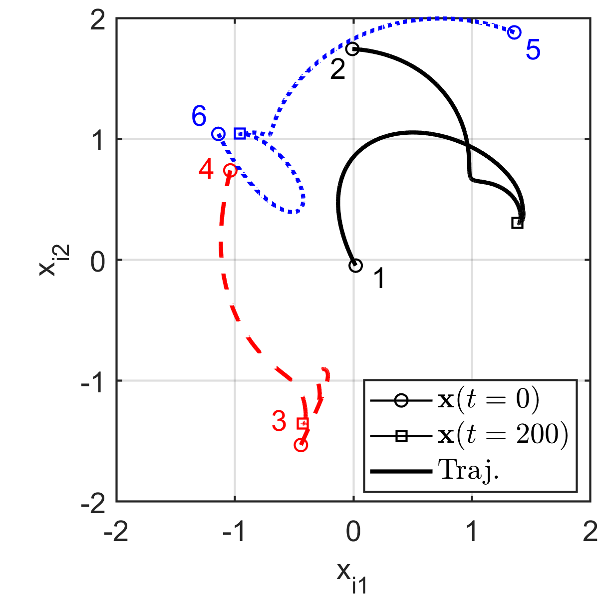
(a) $\mathbf{x}_{i}(t)$

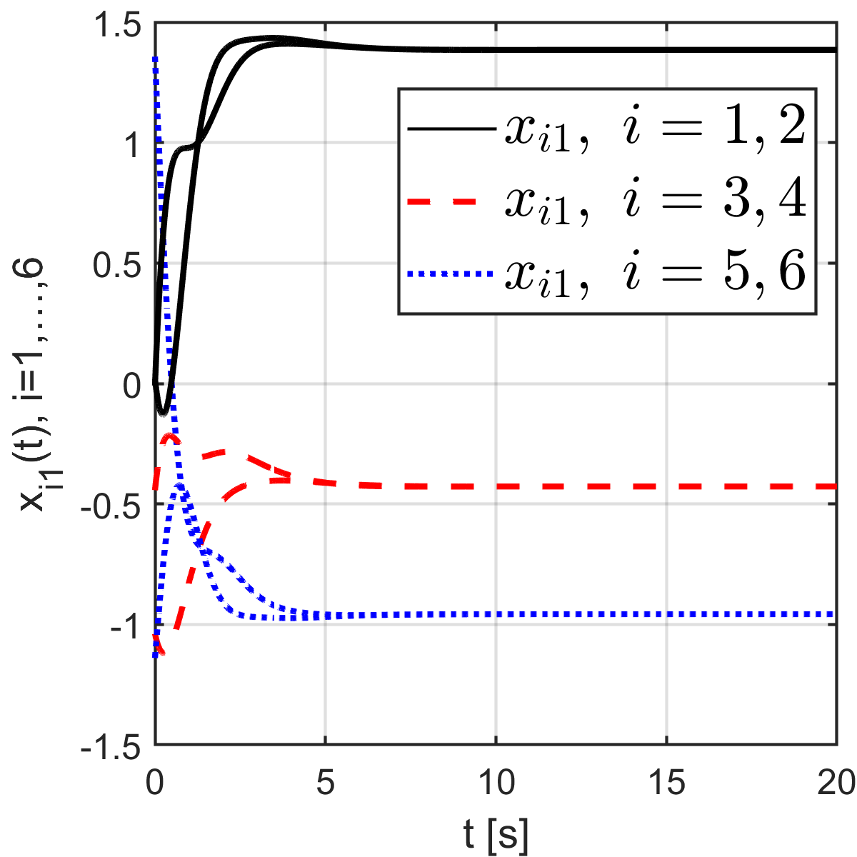
(b) $x_{i1}(t)$

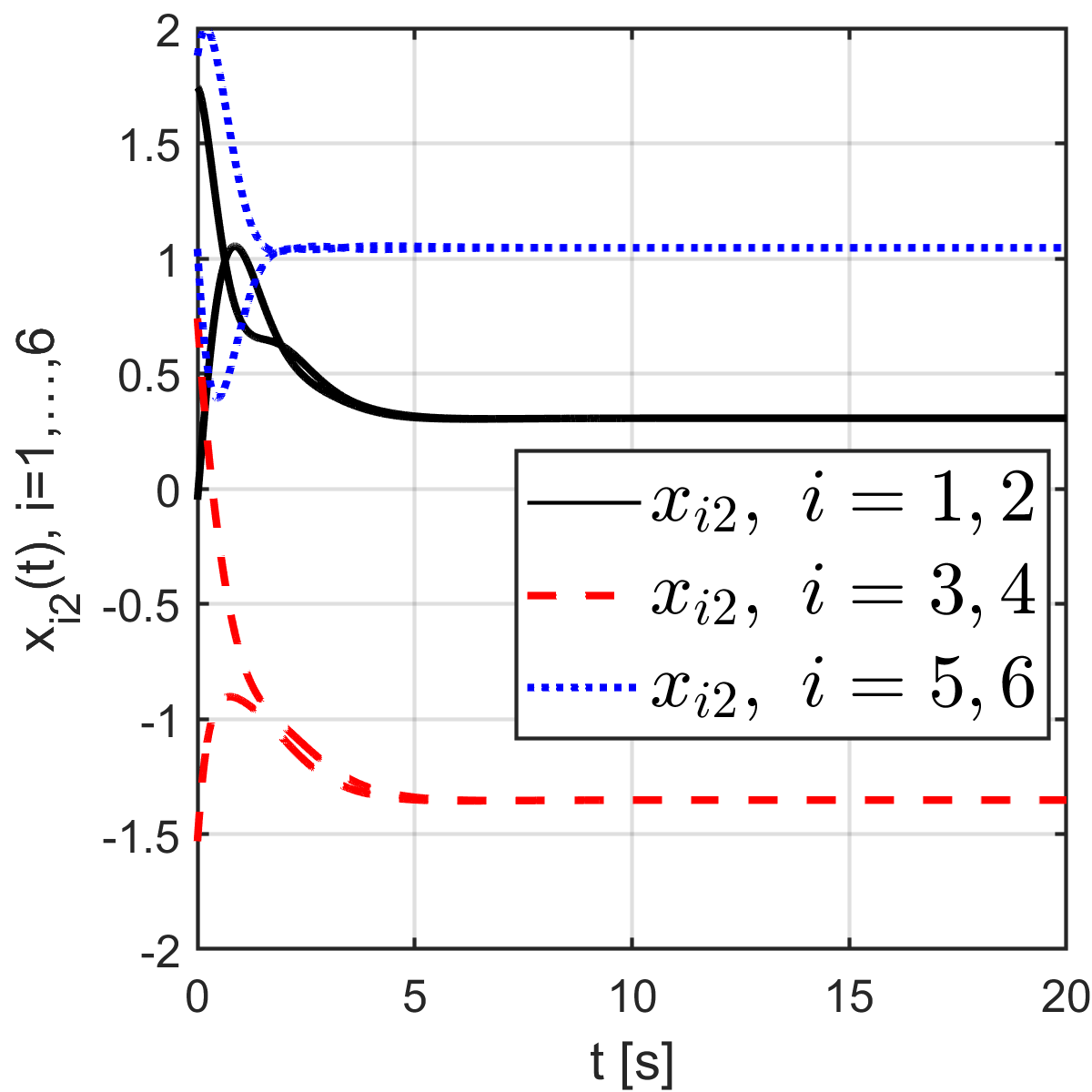
(c) $x_{i2}(t)$

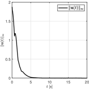
(d) $\|\mathbf{u}\|_{\infty}$

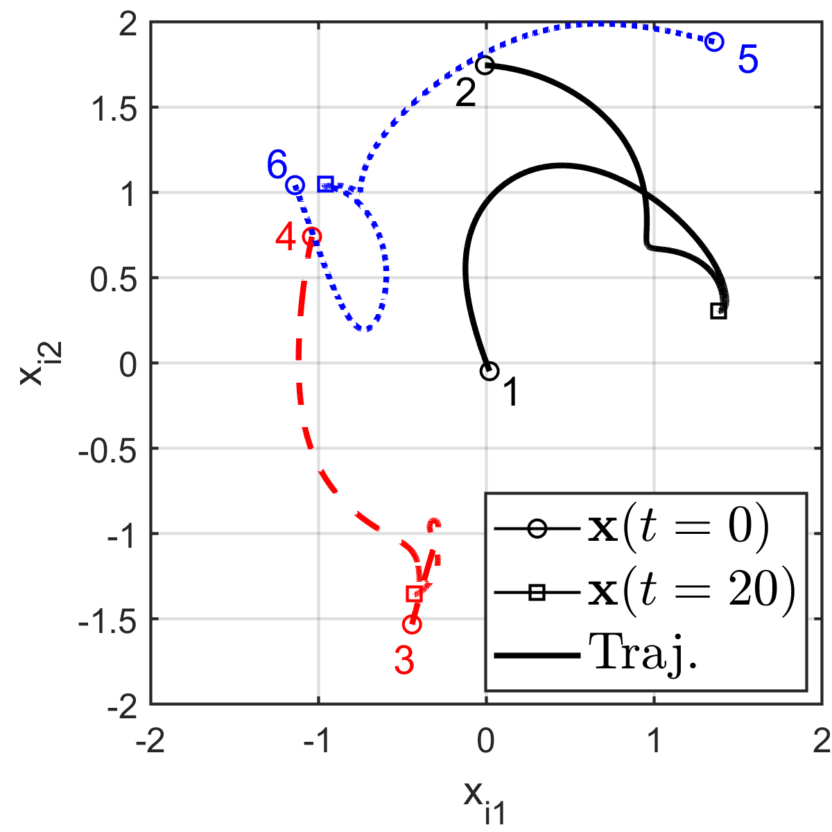
(e) $\mathbf{x}_{i}(t)$

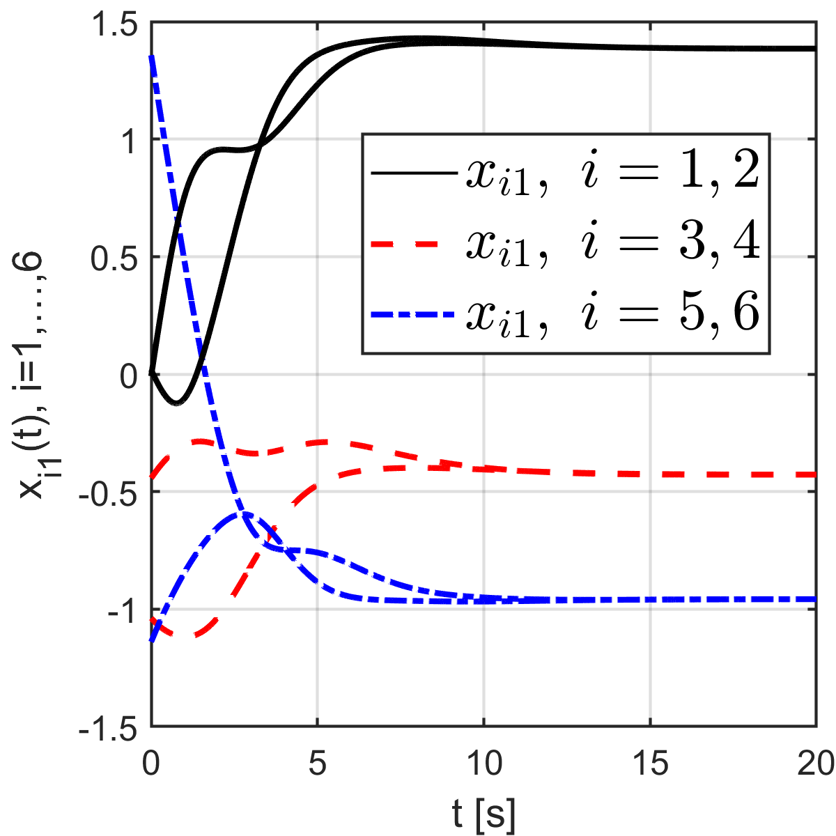
(f) $x_{i1}(t)$

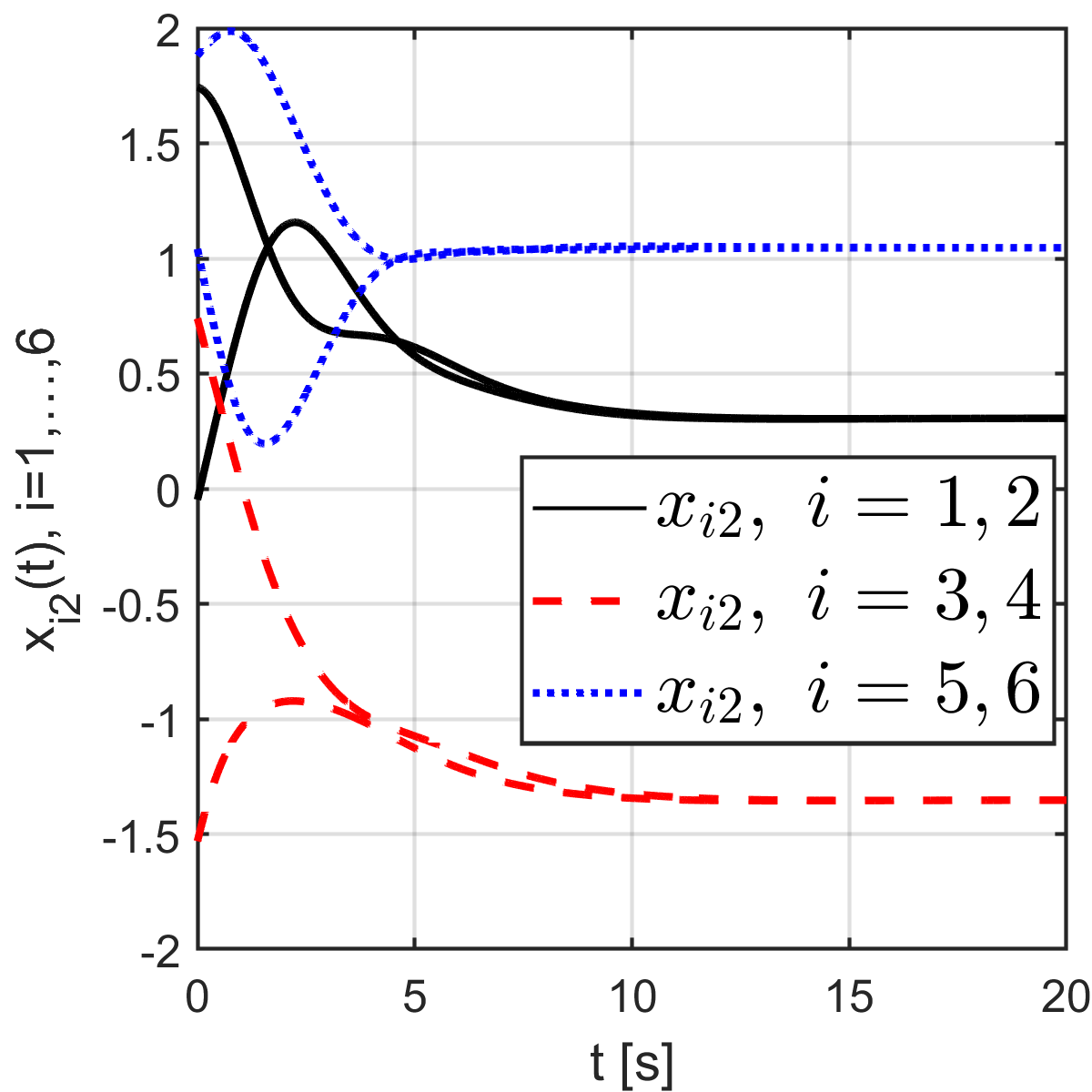
(g) $x_{i2}(t)$

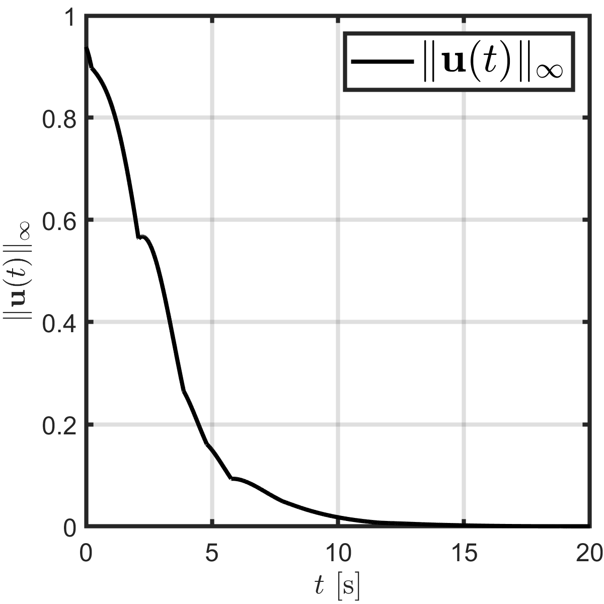
(h) $\|\mathbf{u}\|_{\infty}$

Figure 1: The agents converge to three clusters in 2D under the matrix-scaled consensus algorithms (9) (Figs. (a)–(d)) and (14) (Figs. (e)–(h)).

In this section, we provide simulations of the theoretical results in Sections III, IV. In all simulations, a six-agent system in the two dimensional space ($d=2$) is considered. The interaction between agents are captured by an undirected cycle of six vertices. Denote the SO(2) rotation matrix of angle $\theta$ (rad) by $\mathbf{R}(\theta)=\begin{bmatrix}\cos(\theta)&-\sin(\theta)\\ \sin(\theta)&\cos(\theta)\end{bmatrix}$. The scaling matrices are chosen as $\mathbf{S}_{1}=\mathbf{S}_{2}=\mathbf{R}(\frac{\pi}{3})$ (positive definite), $\mathbf{S}_{3}=\mathbf{S}_{4}=-\mathbf{I}_{2}$ (negative definite), and $\mathbf{S}_{5}=\mathbf{S}_{6}=\mathbf{R}(\frac{5\pi}{3})$ (positive definite).

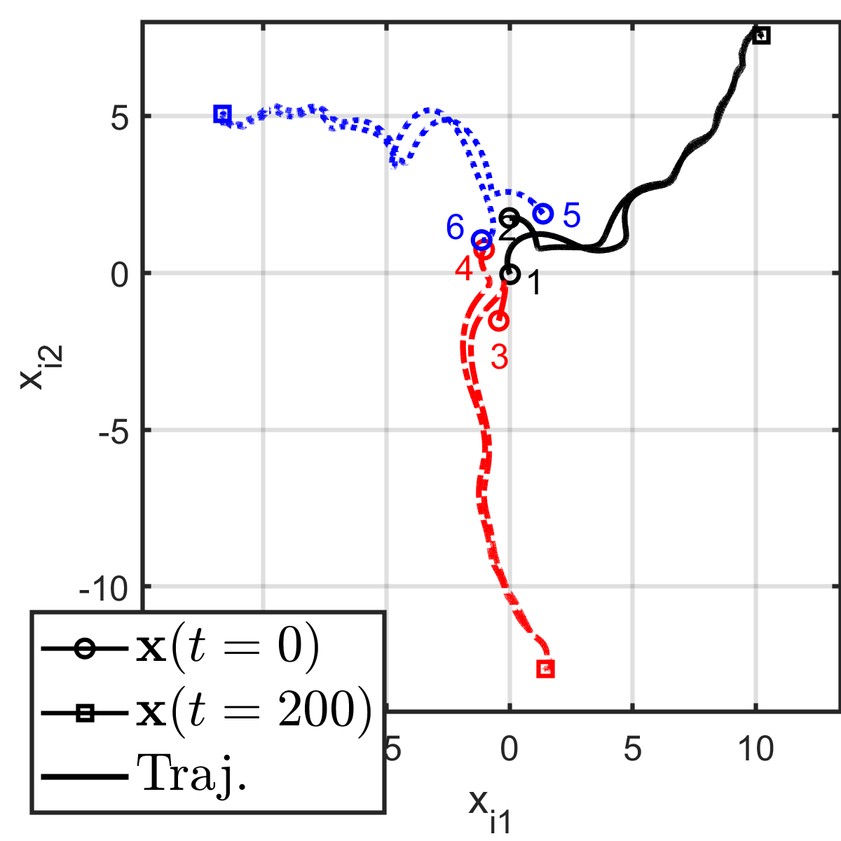
(a) $\mathbf{x}_{i}(t)$

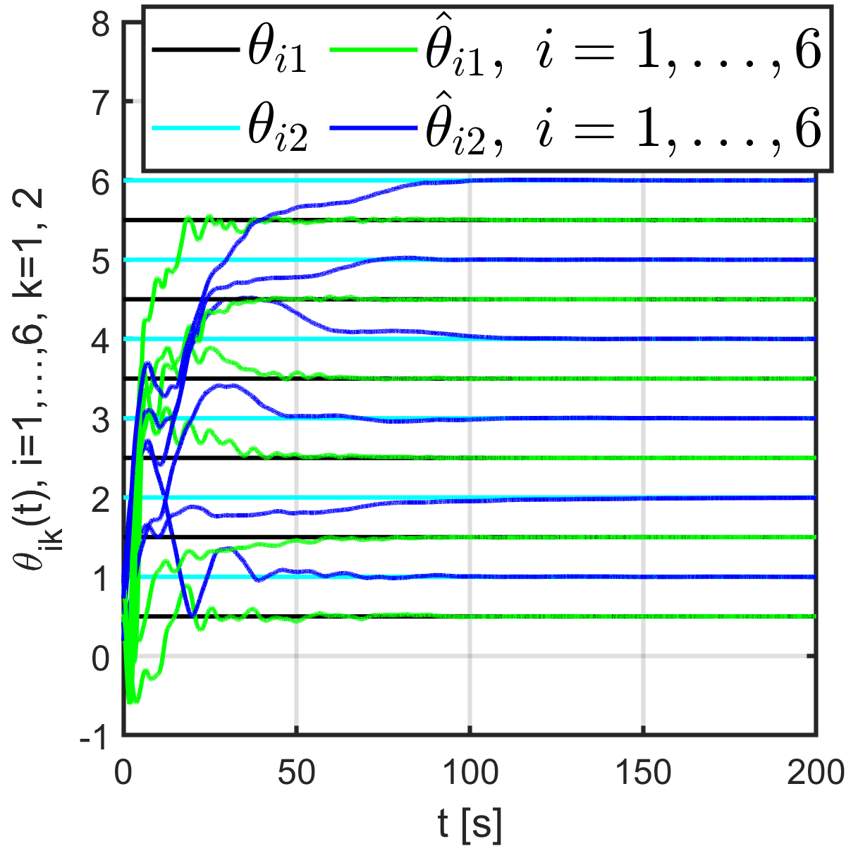
(b) $\bm{\theta}_{i}(t),\hat{\bm{\theta}}_{i}(t)$

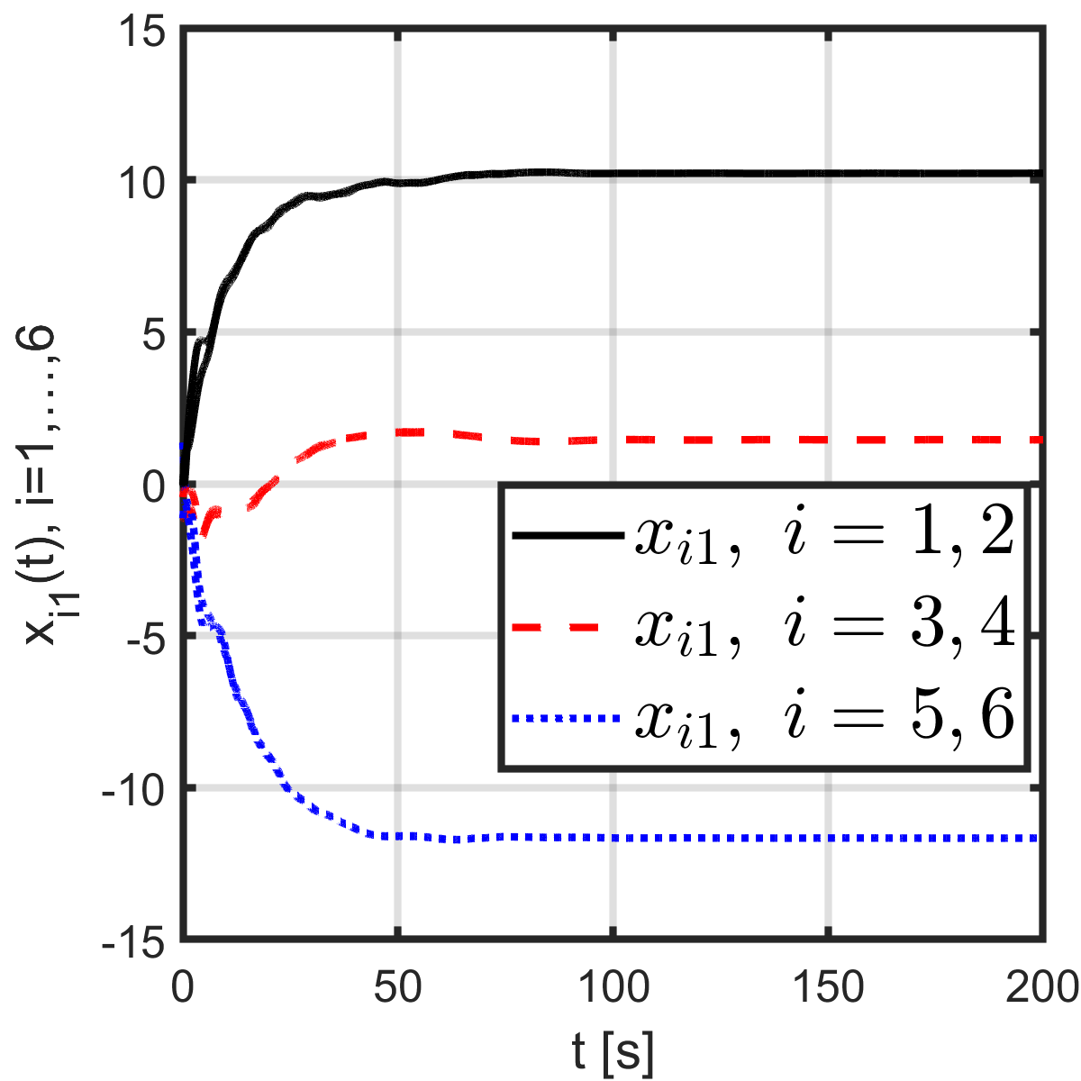
(c) $x_{i1}(t)$

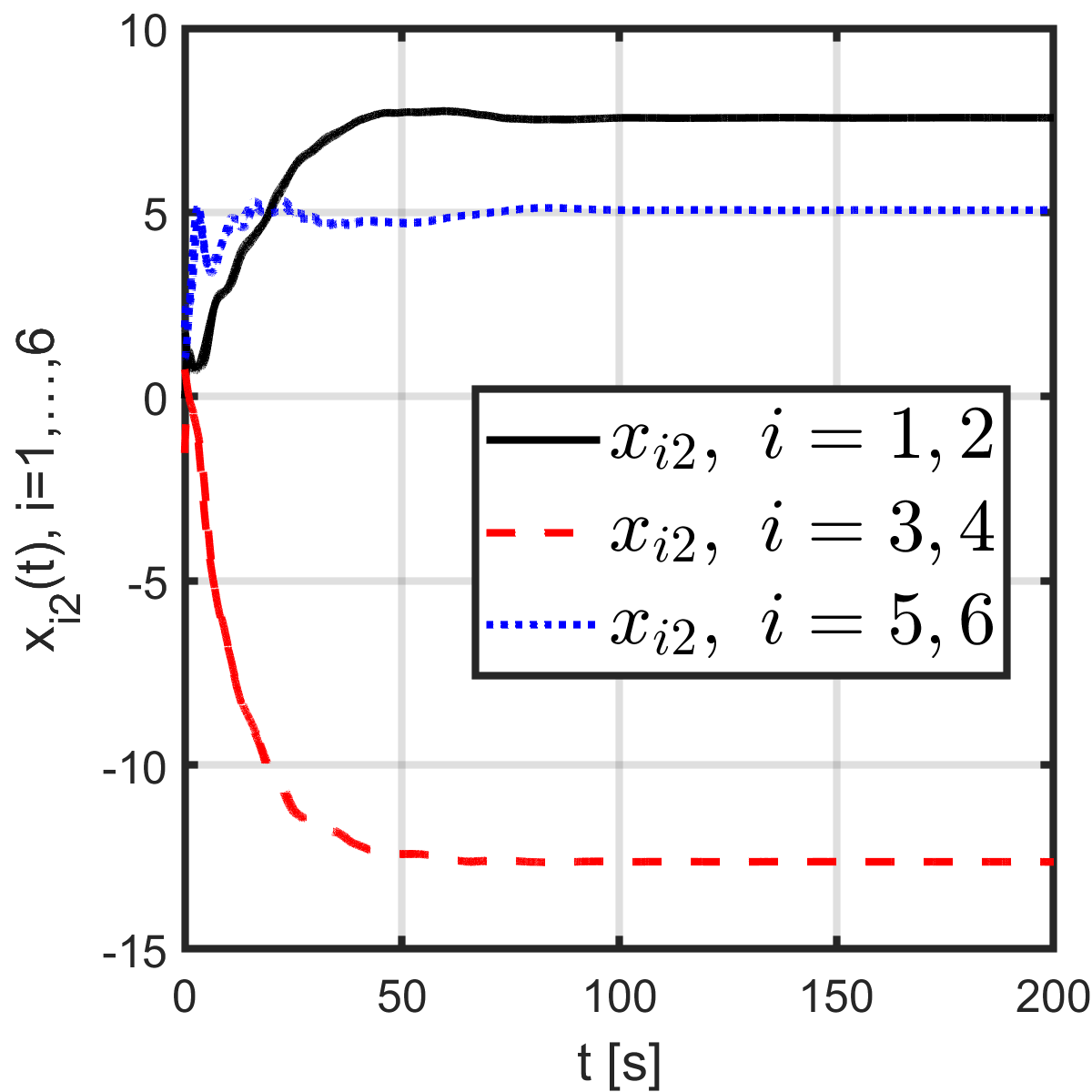
(d) $x_{i2}(t)$

Figure 2: The six-agent system under the adaptive algorithm (16a)–(16b).

V-A Matrix-scaled consensus of single integrators

Figures 1 (a)–(d) shows a simulation of the six-agent system under the matrix-scaled consensus algorithm (9) for 20 seconds, where the initial condition $\mathbf{x}(0)$ was randomly selected. The agents’ trajectories asymptotically converge to three clusters in 2D, which are vertices of an equilateral triangle.

Next, we consider the six-agent system under the nonlinear matrix-scaled algorithm (14) with the same initial state $\mathbf{x}(0)$. We would like the input of each agent to satisfy $\|\mathbf{u}_{i}(t)\|_{\infty}<\beta=1$. This objective is achieved by selecting $\mathbf{f}(\cdot)=(\max_{i}|N_{i}|)^{-1}\text{tanh}(\cdot)=0.5\text{tanh}(\cdot)$. Simulation results are depicted in Figs. 1(e)–(h). Observe that $\mathbf{x}(t)$ converges to the same point as the previous simulation, $\|\mathbf{u}_{i}\|_{\infty}\leq 1,\forall t\geq 0$, the settling time (which is defined as the first time $\mathbf{x}(t)$ enters without escaping $B_{5\%}=\{\|\mathbf{x}(t)-\lim_{t\to+\infty}\mathbf{x}(t)\|<0.05\}$) becomes larger (approx. 10 sec in comparison with 5 sec).

V-B Matrix-scaled consensus of single-integrators with uncertain parameters

Next, we consider a system consisting of 6-single-integrator agents with parametric uncertainties

$$\bm{\phi}_{i}(t)=\begin{bmatrix}0.2\sin(t)&0.5-0.2\sin(\frac{it}{\pi})\\ -0.2\sin(\frac{t}{i\pi})&0.1\cos(\frac{t}{\pi})\end{bmatrix},~{}i=1,\ldots,6,$$

which satisfy the persistently exciting condition, and $\gamma_{i}>0$ are randomly chosen between $[1,10]$. The constant unknown parameters are $\bm{\theta}_{i}=[i-0.5,~{}i]^{\top}$, and the initial estimates $\hat{\bm{\theta}}_{i}(0)$ are randomly generated. Simulation results depicted in Fig. 2 show that $\mathbf{x}_{i}\to\mathcal{C}_{S}$, $\hat{\bm{\theta}}_{i}(t)\approx\bm{\theta}_{i}$ at $t=200$ seconds (Fig. 2 (b)). Due to the unknown parameters, the convergence rate, however, is much slower in comparison with the ideal case.

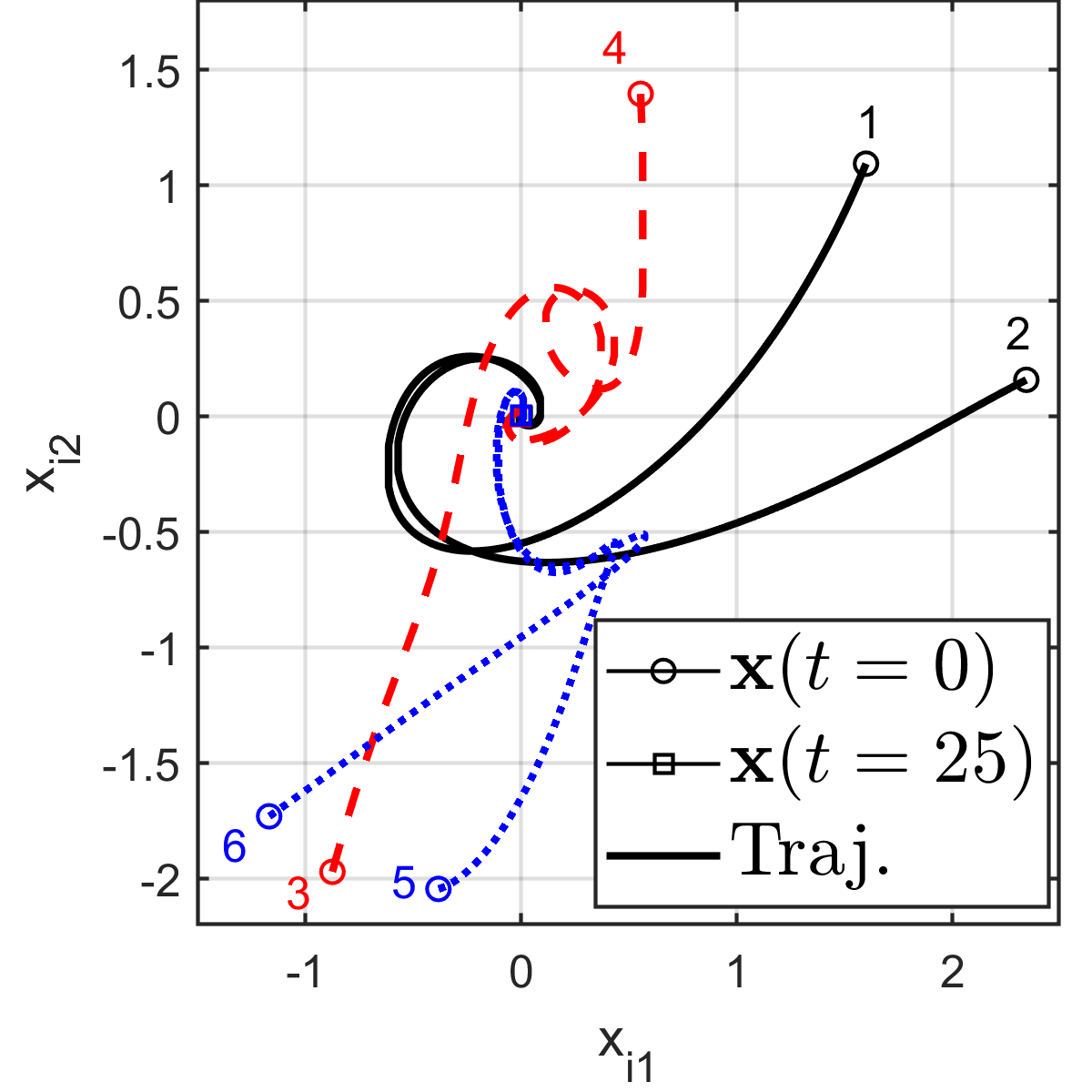
(a) $\mathbf{A}$ is Hurwitz.

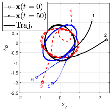
(b) $\mathbf{A}$ has a pair of imaginary eigenvalues, $\mathbf{A}+\mathbf{A}^{\top}\neq\mathbf{0}_{d\times d}$.

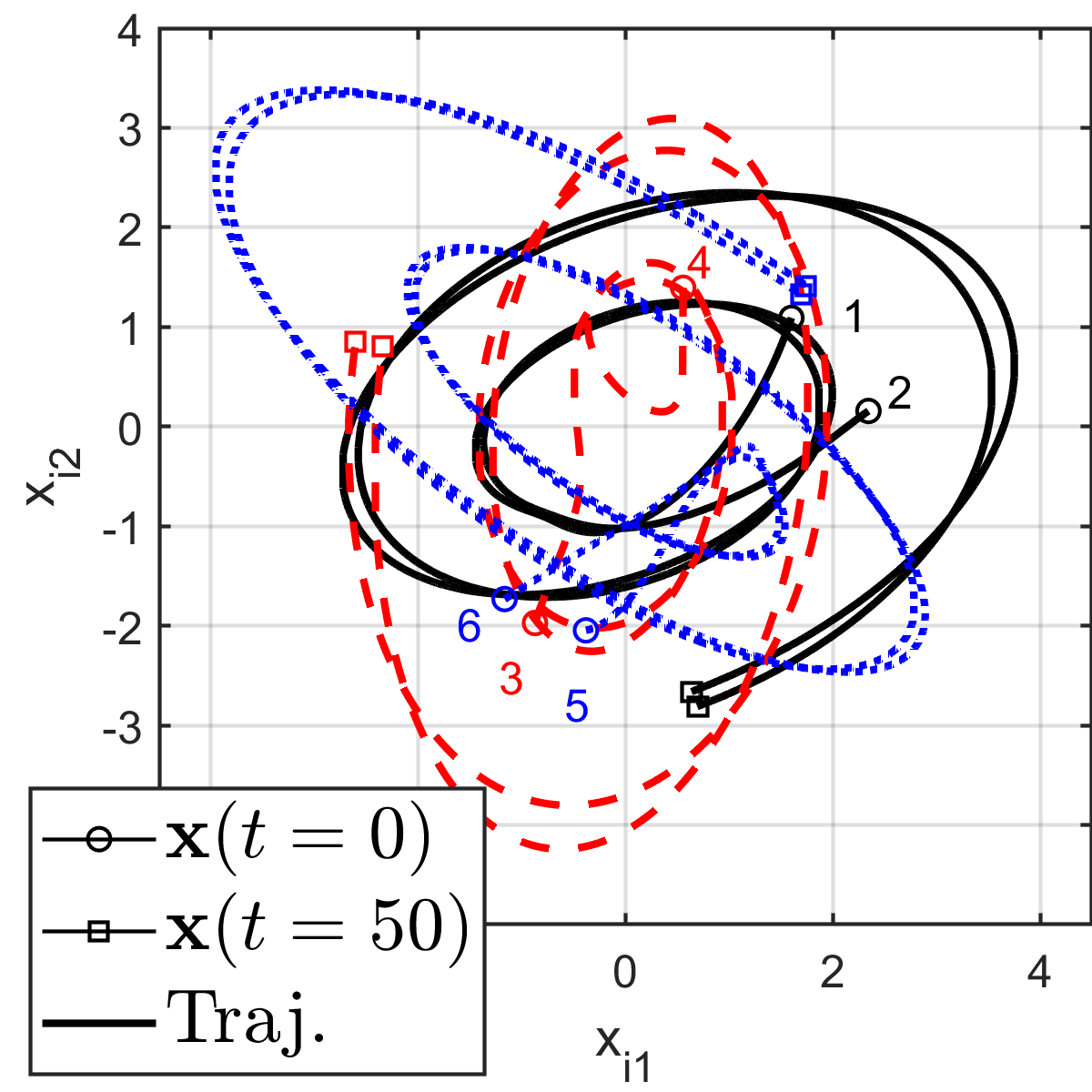
(c) $\mathbf{A}$ is unstable.

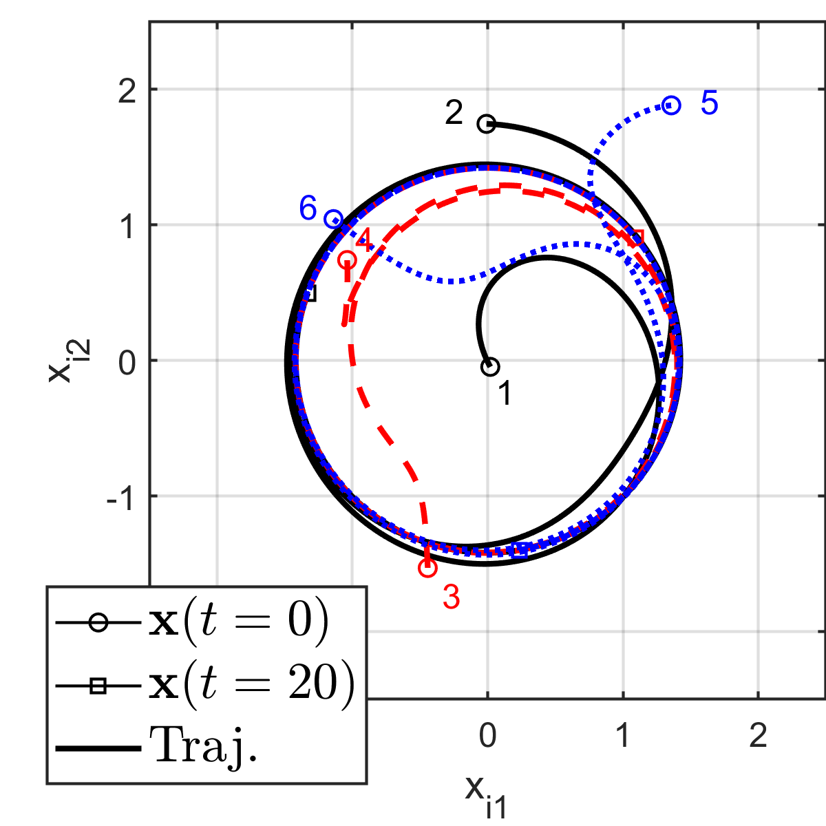
(d) $\mathbf{A}=-\mathbf{A}^{\top}$ and has a pair of imaginary eigenvalues.

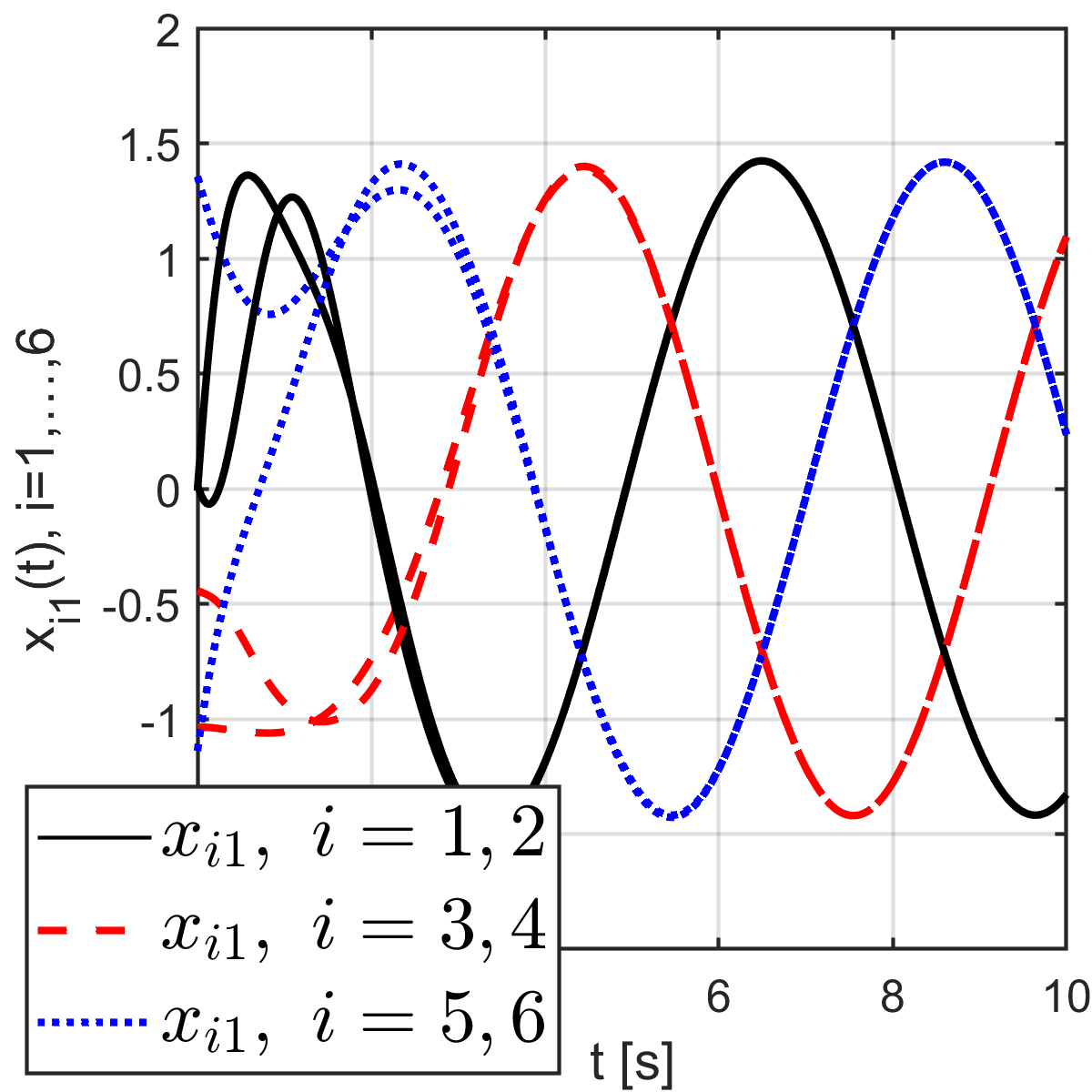
(e) State variables $x_{i1}(t)$ corresponding to trajectories in (d).

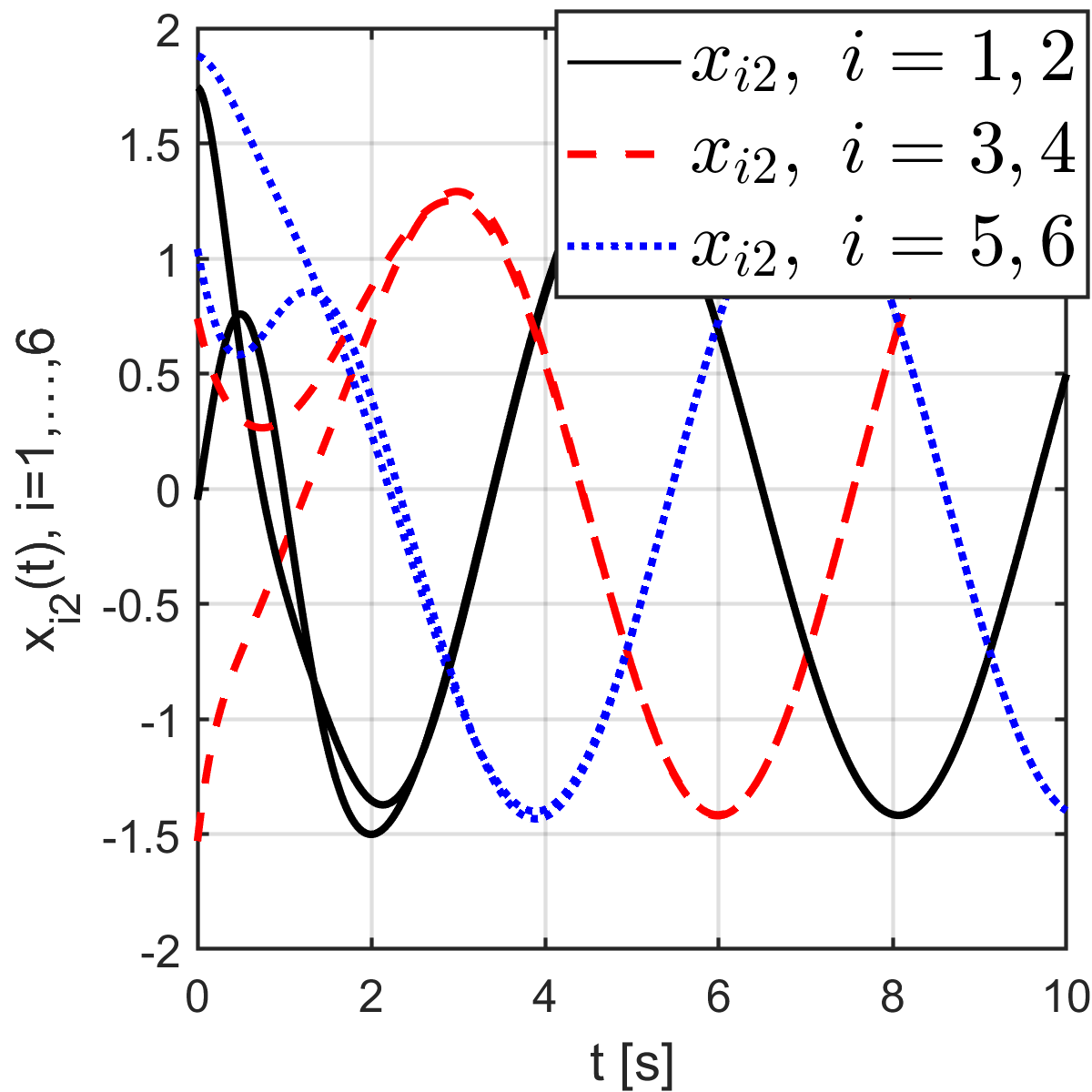
(f) State variables $x_{i2}(t)$ corresponding to trajectories in (d).

Figure 3: The six-agent system modeled by the simplified linear model (21) with different choices of the matrix $\mathbf{A}$.

V-C Matrix-scaled consensus of simplified linear dynamical agents

We simulate the matrix-scaled consensus algorithm for the six-agent system with the simplified linear model (21) for different matrices $\mathbf{A}$ as follows

• $\mathbf{A}=0.5\begin{bmatrix}-1&1\\ -1&0\end{bmatrix}$ has eigenvalues $-0.25\pm\frac{\sqrt{3}}{4}\imath$,

• $\mathbf{A}=\begin{bmatrix}0&1\\ -1&0\end{bmatrix}$ is skew-symmetric, has eigenvalues $\pm\imath$,

• $\mathbf{A}=0.5\begin{bmatrix}0&1\\ -0.5&0\end{bmatrix}$ has a pair of imaginary eigenvalues, $\mathbf{A}$ is not skew-symmetric,

• $\mathbf{A}=0.5\begin{bmatrix}1&1\\ -1&0\end{bmatrix}$ has eigenvalues $0.25\pm\frac{\sqrt{3}}{4}\imath$,

where $\imath^{2}=-1$. In this subsection, the coupling gain is chosen as $c=2$.

Simulation results depicted in Fig. 3 show that the agents’ trajectories are affected by both the unforced dynamics (determined by $\mathbf{A}\mathbf{x}_{i}$) and the matrix-scaled consensus algorithm. Clearly, if $\mathbf{A}$ is stable (unstable), all agents’ states converge to 0 (resp., grow unbounded). In case $\mathbf{A}$ is marginally stable, the agents asymptotically reach a matrix scaled consensus with regard to a trajectory of the system $\dot{\mathbf{r}}=\mathbf{P}\mathbf{A}\mathbf{P}^{-1}\mathbf{r}$. In case $\mathbf{A}$ is skew-symmetric, agents move on a circle centered at the origin, and if $\mathbf{A}$ is not skew-symmetric, agents with the same scaling matrix move on a same elliptical trajectory. Each trajectory of $\mathbf{x}_{i}(t)$ differs from a common solution of $\dot{\mathbf{r}}=\mathbf{P}\mathbf{A}\mathbf{P}^{-1}\mathbf{r}$ by the scaling matrix $\mathbf{S}_{i}$.

V-D Matrix-scaled consensus of general homogeneous linear dynamical agents

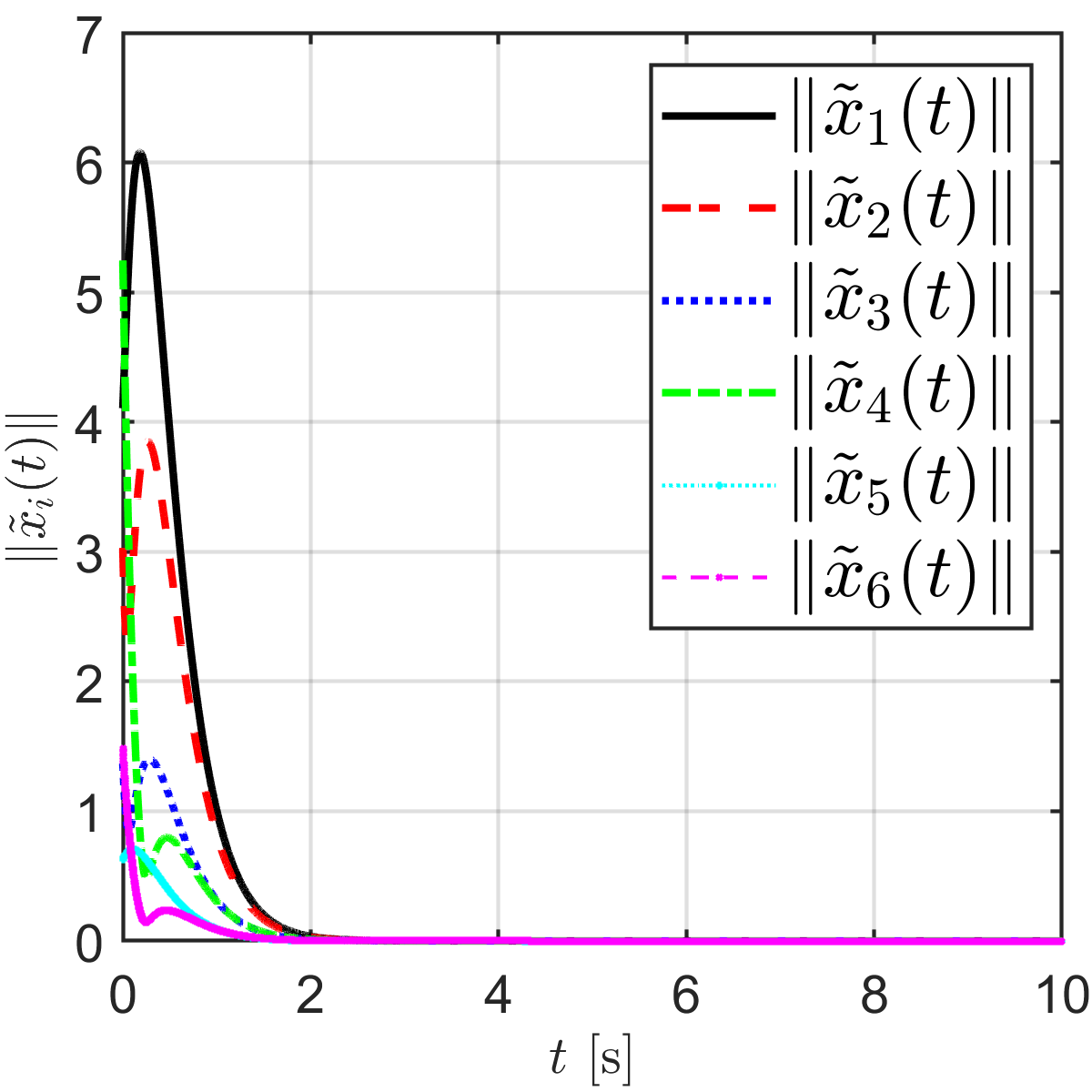
(a) $\|\hat{\mathbf{x}}_{i}(t)\|$

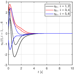
(b) $\eta_{i1}(t)$

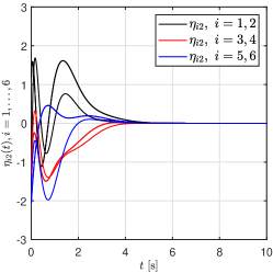
(c) $\eta_{i2}(t)$

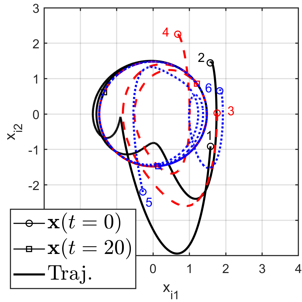
(d) $\mathbf{x}_{i}$

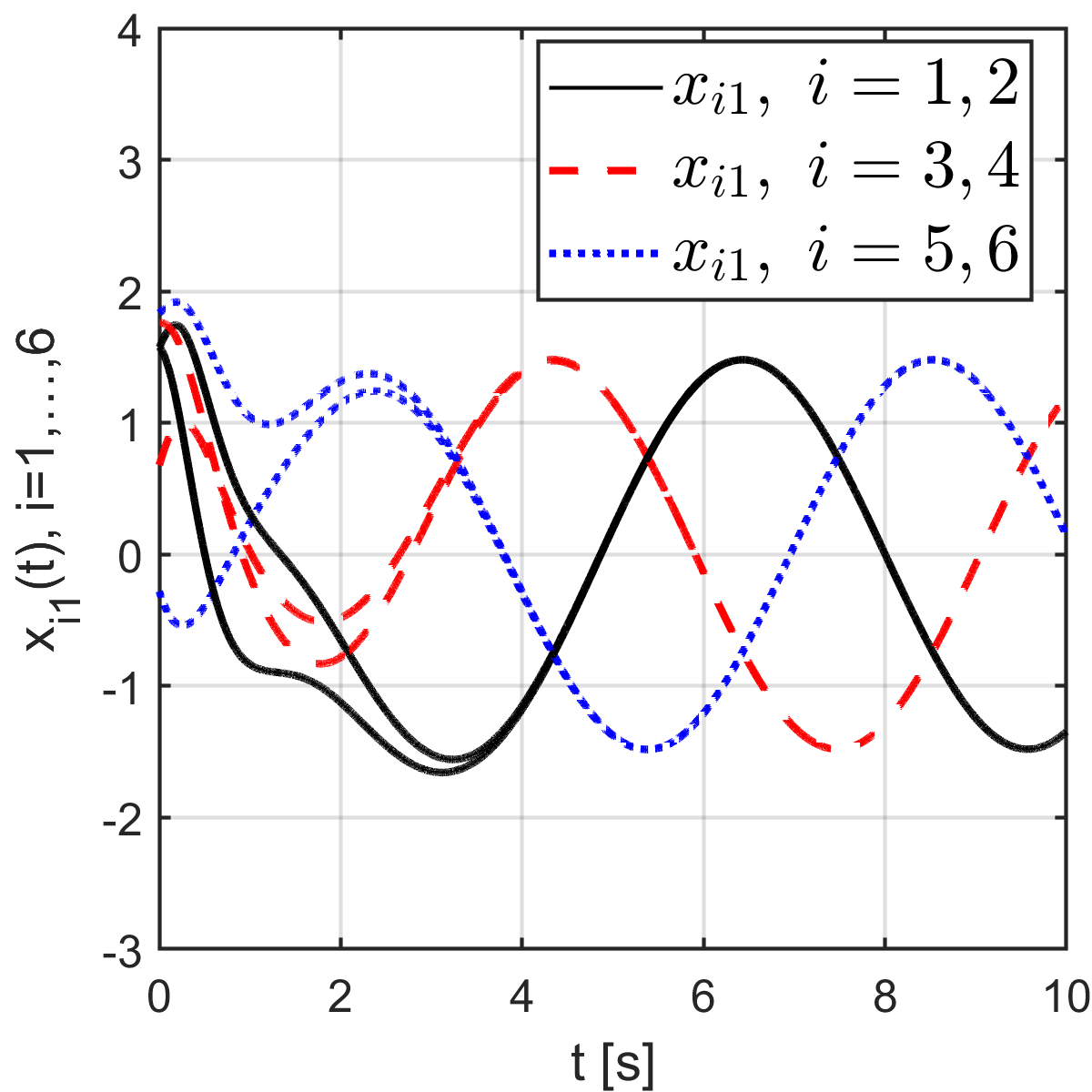
(e) ${x}_{i1}$

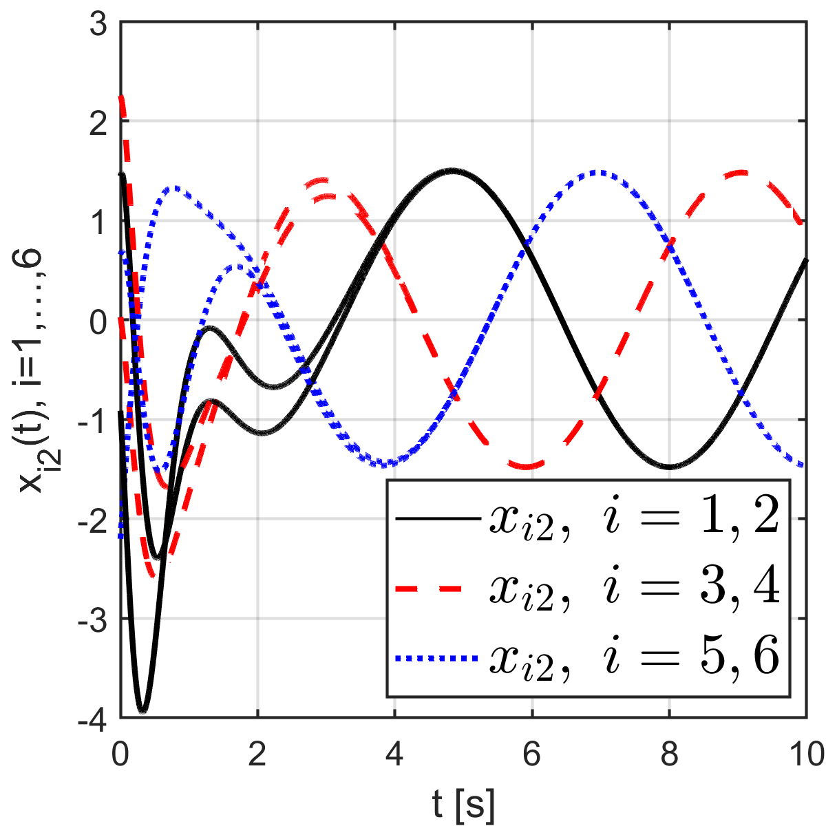
(f) ${x}_{i2}$

Figure 4: Simulations of the homogeneous linear agent system (30) under the matrix-scaled consensus algorithm (25).

In this subsection, let the agent be modeled by a linear oscillator with a control input

$$\dot{x}_{i1} =x_{i2},$$ (30a)

$$\dot{x}_{i2} =-\omega^{2}x_{i1}+u_{i},$$ (30b)

$$y_{i} =x_{i1},~{}\,i=1,\ldots,6,$$ (30c)

and $\omega=1$. The corresponding system matrices are $\mathbf{A}=\begin{bmatrix}0&1\\ -1&0\end{bmatrix}$, $\mathbf{B}=\begin{bmatrix}0\\ 1\end{bmatrix}$, $\mathbf{C}=[1,~{}0]$, $\mathbf{K}=[-3,-4]$, $\mathbf{H}=[-8,-15]^{\top}$, and $c=2$. Simulation corresponding to a randomly generated initial condition is displayed in Fig. 4. The state estimate error $\tilde{\mathbf{x}}_{i}=\hat{\mathbf{x}}_{i}-\mathbf{x}_{i}$ and the auxiliary variable $\bm{\eta}$ vanish exponentially fast. Figures 4(d), (e), (f) depict the trajectories of 6 agents; Each agent’s trajectory differ to a common solution of $\dot{\mathbf{r}}=\mathbf{P}\mathbf{A}\mathbf{P}^{-1}\mathbf{r}$ by its scaling matrix.

V-E Matrix-scaled consensus of general heterogeneous linear dynamical agents

Consider a system of six heterogeneous linear agents, where matrix $\mathbf{A}$ is the same as in the previous subsection, $\bar{\mathbf{A}}_{i}$ are randomly generated with entries belong to $[-0.2,~{}0.2]$. The matrices $\mathbf{B}_{i}=\mathbf{B}+\bm{\Delta}_{B}$, where $\bm{\Delta}_{B}=\begin{bmatrix}0&\delta_{b_{i}}\end{bmatrix}^{\top}$, with $\delta_{b_{i}}$ be randomly generated to take values on the interval $[-0.5,0.5]$, and $\mathbf{C}_{i}=\mathbf{C},~{}~{}\forall i=1,\ldots,n$. The matrices $\mathbf{K}_{i}$ and $\mathbf{H}_{i}$ are designed so that each matrix $\mathbf{A}_{i}+\mathbf{B}_{i}\mathbf{K}_{i}$ have eigenvalues $-2,-2$ and each matrix $\mathbf{A}_{i}+\mathbf{H}_{i}\mathbf{C}_{i}$ have eigenvalues $-4,-4$, for $i=1,\ldots,6$. The control gains are given as $c=2$, $\beta_{1}=2$ and $\beta_{2}=5$.

Figures 5(a), (b), (c) show that $\mathbf{x}(t)\to\mathcal{C}_{S}$ asymptotically under the algorithm (29). The system eventually achieves matrix-scaled consensus on a trajectory of $\dot{\mathbf{r}}=\mathbf{P}\mathbf{A}\mathbf{P}^{-1}\mathbf{r}$. For comparison, the same heterogeneous system is simulated without using the control law (29). Without the signum terms, Fig. 5(d), (e), (f) show that the system diverges. Thus, simulation results are consistent with the analysis.

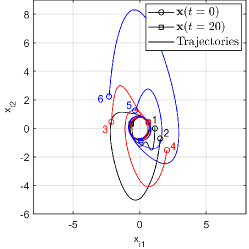
(a) $\mathbf{x}_{i}$

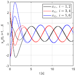
(b) $x_{i1}$

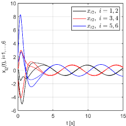
(c) $x_{i2}$

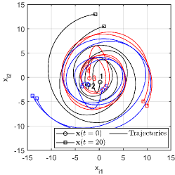
(d) $\mathbf{x}_{i}$

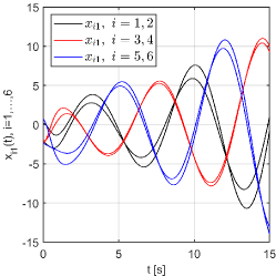
(e) $x_{i1}$

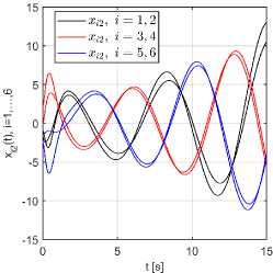
(f) $x_{i2}$

Figure 5: Simulation of the heterogeneous linear systems when the agents: (i) employ the algorithm (29): (a), (b), (c); and (ii) do not include the signum term in $\hat{\mathbf{u}}$ in (29): (d), (e), (f).

VI Conclusions

In this paper, the matrix-scaled consensus model has been proposed and studied in detail. Several matrix-scaled consensus algorithms were designed for linear agents interacting over an undirected network. The asymptotic behaviors of the proposed algorithms associate with the algebraic properties of the matrix-scaled Laplacian $(\text{sign}(\mathbf{S})\mathbf{L}\otimes\mathbf{I}_{d})\mathbf{S}$. Main difficulties in the stability analysis comes from the asymmetry and multi-dimensionality of the matrix-scaled Laplacian.

As the study of the matrix-scaled consensus algorithm in this paper also focused on undirected graphs and linear agents, further research will consider the matrix-scaled consensus algorithm with directed or signed graphs.

Appendix A Asymptotic behavior of an adaptive system

Lemma A.1

[32] Given the system in the following form

$$\dot{\mathbf{x}}_{1} =\mathbf{h}(t)\mathbf{x}_{2}+\bm{\varphi}(t),~{}\mathbf{x}_{1}\in\mathbb{R}^{n},~{}\mathbf{x}_{2}\in\mathbb{R}^{m},$$ (31a)

$$\dot{\mathbf{x}}_{2} =\bm{\psi}(t),$$ (31b)

where the functions $\mathbf{h}:\mathbb{R}^{+}\to\mathbb{R}^{n\times m}$, $\bm{\varphi}:\mathbb{R}^{+}\to\mathbb{R}^{n}$, and $\bm{\psi}:\mathbb{R}^{+}\to\mathbb{R}^{m}$ are such that (i) $\lim_{t\to+\infty}\|\mathbf{x}_{1}(t)\|=\lim_{t\to+\infty}\|\bm{\varphi}(t)\|=\lim_{t\to+\infty}\|\bm{\psi}(t)\|={0}$, (ii) $\mathbf{h}(t)$, $\dot{\mathbf{h}}(t)$ are bounded and (iii) there exist positive constants $T,\mu_{1},\mu_{2}$ and $l$ such that for all $t\geq 0$, $\mu_{1}\mathbf{I}_{n}\geq\int_{t}^{t+T}\mathbf{h}(\tau)^{\top}\mathbf{h}(\tau)d\tau\geq\mu_{2}\mathbf{I}_{n}$, then $\lim_{t\to+\infty}\|\mathbf{x}_{2}(t)\|=0$.

Appendix B Proof of Lemma IV.1

Let $\bm{\Theta}_{c}=c\mathbf{\Theta}+\bm{\Delta}_{\Theta}$, and consider the dynamical system

$$\dot{\mathbf{x}}=\bm{\Theta}_{c}\mathbf{x}.$$

Consider the Lyapunov function $V=\mathbf{x}^{\top}\mathbf{Q}\mathbf{x}$, we have, $\dot{V}=\mathbf{x}^{\top}(\mathbf{Q}\bm{\Theta}_{c}+\bm{\Theta}_{c}^{\top}\mathbf{Q})\mathbf{x}=-c\|\mathbf{x}\|^{2}+2\mathbf{x}^{\top}\mathbf{Q}\bm{\Delta}_{\Theta}\mathbf{x}\leq-(c-2\|\mathbf{Q}\|\|\bm{\Delta}_{\Theta}\|)\|\mathbf{x}\|^{2}\leq-(c-2{\delta}_{\Theta}\lambda_{\max}(\mathbf{Q}))\lambda_{\min}^{-1}(\mathbf{Q})V.$ Thus, $\mathbf{x}(t)$ is globally exponentially stable. Equivalently, the matrix $\bm{\Theta}_{c}$ is Hurwitz.

References

• [1] Olfati-Saber, Fax, and Murray, “Consensus and cooperation in networked multi-agent systems,” Proceedings of the IEEE, vol. 95, no. 1, pp. 215–233, 2007.
• [2] W. Ren, R. W. Beard, and E. M. Atkins, “Information consensus in multivehicle cooperative control,” IEEE Control Systems Magazine, vol. 27, no. 2, pp. 71–82, 2007.
• [3] A. Proskurnikov and R. Tempo, “A tutorial on modeling and analysis of dynamic social networks: Part I,” Annual Reviews in Control, vol. 43, pp. 65–79, 2017.
• [4] S. Roy, “Scaled consensus,” Automatica, vol. 51, pp. 259–262, 2015.
• [5] D. Meng and Y. Jia, “Scaled consensus problems on switching networks,” IEEE Transactions on Automatic Control, vol. 61, no. 6, pp. 1664–1669, 2015.
• [6] ——, “Robust consensus algorithms for multiscale coordination control of multivehicle systems with disturbances,” IEEE Transactions on Industrial Electronics, vol. 63, no. 2, pp. 1107–1119, 2015.
• [7] H. D. Aghbolagh, E. Ebrahimkhani, and F. Hashemzadeh, “Scaled consensus tracking under constant time delay,” IFAC-PapersOnLine, vol. 49, no. 22, pp. 240–243, 2016.
• [8] Y. Shang, “On the delayed scaled consensus problems,” Applied Sciences, vol. 7, no. 7, p. 713, 2017.
• [9] K. Hanada, T. Wada, I. Masubuchi, T. Asai, and Y. Fujisaki, “On a new class of structurally balanced graphs for scaled group consensus,” in Proc. of the 58th Annual Conf. Soc. Instrument Control Eng. Japan (SICE), 2019, pp. 1671–1676.
• [10] Y. Wu, J. Hu, Y. Zhao, and B. K. Ghosh, “Adaptive scaled consensus control of coopetition networks with high-order agent dynamics,” International Journal of Control, vol. 94, no. 4, pp. 909–922, 2021.
• [11] Y. Chen, Z. Zuo, and Y. Wang, “Scaled consensus over a network of wave equations,” IEEE Transactions on Control of Network Systems, vol. 9, no. 3, pp. 1385–1396, 2022.
• [12] W. Ren, “Collective motion from consensus with Cartesian coordinate coupling,” IEEE Transactions on Automatic Control, vol. 54, no. 6, pp. 1330–1335, 2009.
• [13] J. Ramirez-Riberos, M. Pavone, E. Frazzoli, and D. W. Miller, “Distributed control of spacecraft formations via cyclic pursuit: Theory and experiments,” Journal of Guidance, Control, and Dynamics, vol. 33, no. 5, pp. 1655–1669, 2010.
• [14] Q. V. Tran, M. H. Trinh, and H.-S. Ahn, “Surrounding formation of star frameworks using bearing-only measurements,” in Proc. of the European Control Conference, Lismason, Cyprus, 2018, pp. 368–373.
• [15] B.-H. Lee, S.-M. Kang, and H.-S. Ahn, “Distributed orientation estimation in so ($d$) and applications to formation control and network localization,” IEEE Transactions on Control of Network Systems, vol. 6, no. 4, pp. 1302–1312, 2018.
• [16] H.-S. Ahn and M. H. Trinh, “Consensus under biased alignment,” Automatica, vol. 110, p. 108605, 2019.
• [17] M. H. Trinh, D. V. Vu, Q. V. Tran, and H.-S. Ahn, “Matrix-scaled consensus,” in Proc. of the 61st IEEE Conference on Decision and Control (CDC).   IEEE, 2022, pp. 346–351.
• [18] L. Scardovi and R. Sepulchre, “Synchronization in networks of identical linear systems,” Automatica, vol. 45, no. 11, pp. 2557–2562, 2009.
• [19] H. Kim, H. Shim, and J. H. Seo, “Output consensus of heterogeneous uncertain linear multi-agent systems,” IEEE Transactions on Automatic Control, vol. 56, no. 1, pp. 200–206, 2010.
• [20] Z. Li, Z. Duan, G. Chen, and L. Huang, “Consensus of multiagent systems and synchronization of complex networks: A unified viewpoint,” IEEE Transactions on Circuits and Systems I: Regular Papers, vol. 57, no. 1, pp. 213–224, 2009.
• [21] Z. Li, W. Ren, L. iu, and L. Xie, “Distributed consensus of linear multi-agent systems with adaptive dynamic protocols,” Automatica, vol. 49, no. 7, pp. 1986–1995, 2013.
• [22] E. Panteley and A. Loría, “Synchronization and dynamic consensus of heterogeneous networked systems,” IEEE Transactions on Automatic Control, vol. 62, no. 8, pp. 3758–3773, 2017.
• [23] S. E. Tuna, “Synchronization under matrix-weighted laplacian,” Automatica, vol. 73, pp. 76–81, 2016.
• [24] D. A. Burbano, R. A. Freeman, and K. Lynch, “A distributed adaptive observer for leader-follower networks,” in Proc. of the American Control Conference (ACC).   IEEE, 2019, pp. 2722–2727.
• [25] M. Mesbahi and M. Egerstedt, Graph Theoretic Methods in Multiagent Networks.   Princeton NJ: Princeton University Press, 2010.
• [26] D. Zelazo and M. Mesbahi, “Edge agreement: Graph-theoretic performance bounds and passivity analysis,” IEEE Transactions on Automatic Control, vol. 56, no. 3, pp. 544–555, 2010.
• [27] M. H. Trinh, C. V. Nguyen, Y.-H. Lim, and H.-S. Ahn, “Matrix-weighted consensus and its applications,” Automatica, vol. 89, pp. 415–419, 2018.
• [28] A. M. Ostrowski, “A quantitative formulation of sylvester’s law of inertia,” Proc. N. A. S, vol. 45, pp. 740–744, 1959.
• [29] M. H. Nguyen and M. H. Trinh, “Leaderless- and leader-follower matrix-weighted consensus with uncertainties,” Measurements, Control and Automation, vol. 3, no. 2, pp. 33–41, 2022.
• [30] J. A. Moreno and M. Osorio., “Strict lyapunov functions for the super-twisting algorithm,” IEEE Transactions on Automatic control, vol. 57, no. 4, pp. 1035–1040, 2012.
• [31] H. K. Khalil, Nonlinear control.   Pearson New York, 2015, vol. 406.
• [32] G. Besançon, “Remarks on nonlinear adaptive observer design,” Systems & Control Letters, vol. 41, no. 4, pp. 271–280, 2000.