Renewal processes linked to fractional relaxation equations with variable order

Abstract.

We introduce and study here a renewal process defined by means of a time-fractional relaxation equation with derivative order $\alpha(t)$ varying with time $t\geq 0$. In particular, we use the operator introduced by Scarpi in the Seventies (see [23]) and later reformulated in the regularized Caputo sense in [4], inside the framework of the so-called general fractional calculus. The model obtained extends the well-known time-fractional Poisson process of fixed order $\alpha\in(0,1)$ and tries to overcome its limitation consisting in the constancy of the derivative order (and therefore of the memory degree of the interarrival times) with respect to time. The variable order renewal process is proved to fall outside the usual subordinated representation, since it can not be simply defined as a Poisson process with random time (as happens in the standard fractional case). Finally a related continuous-time random walk model is analysed and its limiting behavior established.

1. Introduction

The Poisson process and, in general, the renewal processes are extensively studied and applied in many different fields, ranging from physics to finance and actuarial sciences. In particular, their fractional extensions have been proved to be useful since they are characterized by non-exponentially distributed intervals between subsequent renewal times. It is indeed well-known that the time-fractional Poisson process (of order $\alpha\in(0,1]$) is a renewal process with interarrival times following a Mittag-Leffler distribution (with parameter $\alpha$) (see, for example, [1], [16], [19]). The latter entails a withdrawal from the memoryless property, which is greater the further away $\alpha$ is from $1$. Although this model is much more flexible, and adaptable to real data, than the standard one, there is still a rigidity since the derivative order (and therefore the memory degree of the intertimes) is constantly equal to a fixed value $\alpha$ over time.

We introduce and study here a renewal process defined by means of a time-fractional relaxation equation with order $\alpha(t)$ varying with time $t>0$. The class of suitable functions $\alpha(\cdot)$ is characterized and some explanatory examples of choices are given; in particular, $\alpha(\cdot)$ can be modelled to represent two different variable-order processes: a transition from an initial order $\alpha_{1}$ to a second order $\alpha_{2}$ (to be achieved as $t\rightarrow+\infty$); a transition from an initial order $\alpha_{1}$ to a second order $\alpha_{2}$ (to be achieved at a finite time $T$) with a return the initial value $\alpha_{1}$ as $t\rightarrow+\infty$. These models can be compared with the renewal processes defined by means of distributed order derivatives (see [2] and [7]), under the assumption of a discrete uniform distribution for the random order $\alpha$ (i.e., taking values $\alpha_{1}$ and $\alpha_{2}$), even if, in our case, the transition between the two values is depending on the time.

Although different approaches are available in the literature to define variable-order fractional derivatives, in this work we focus on the operator introduced by Scarpi in the Seventies (see [23]) and later reformulated in the regularized Caputo sense in [4]. The main feature of this approach is that it formulates a generalization of classic constant-order operators in the Laplace domain, thus to facilitate the construction of operators satisfying a Sonine condition.

This work is organized in the following way. In Section 2 we introduce the variable-order generalization of the fractional derivative (according to the mentioned approach introduced by Scarpi) and we recall some basic facts about time-fractional Poisson processes of constant order. In Section 3 we consider the variable-order fractional relaxation equation and formulate the basic assumptions needed to guarantee that its solution is a proper tail distribution for the interarrival times of a renewal process. In Section 4 the renewal process defined by means of the previous results is hence studied and some features, such as the factorial moments and the autocovariance, are obtained in the Laplace domain; some graphical representations are provided thanks to numerical inversion of the corresponding Laplace transformations. Section 5 is devoted to the study of the continuous-time random walk with counting process represented by the variable-order fractional renewal and we study its asymptotic behavior, under an appropriate rescaling and under some assumptions on the jumps distribution.

2. Preliminaries

A variable-order fractional derivative can be provided by means of the following definition (we refer to [4] for a more in-depth treatment).

Definition 2.1.

Let $\alpha:[0,T]\rightarrow(0,1),$ $T\in\mathbb{R}^{+}$, be a locally integrable function with Laplace transform $A(s):=\int_{0}^{+\infty}e^{-st}\alpha(t)dt$ and let $\phi_{A}(t),$ $t\in[0,T],$ be the inverse Laplace transform of $\widetilde{\phi}_{A}(s):=s^{sA(s)-1},$ for $s>0$. For $f\in AC[0,T]$ the (Caputo-type) fractional derivative with variable order $\alpha(t)$ is defined as

(2.1) $$D_{t}^{\alpha(t)}f(t):=\int_{0}^{t}\phi_{A}(t-\tau)f^{\prime}(\tau)d\tau,\qquad t\in[0,T].$$

It is easy to check that, for $\alpha(t)=\alpha$ for any $t,$ the operator $D_{t}^{\alpha(t)}$ coincides with the standard Caputo fractional derivative of order $\alpha$, since, in this case, $A(s)=\alpha/s$ and $\widetilde{\phi}_{A}(s)=s^{\alpha-1}.$ Therefore the kernel is $\phi_{\alpha}(t)=t^{-\alpha}/\Gamma(1-\alpha)$ and (2.1) reduces to

$${}^{C}D_{t}^{\alpha}f(t):=\frac{1}{\Gamma(1-\alpha)}\int_{0}^{t}(t-\tau)^{-\alpha}f^{\prime}(\tau)d\tau,\qquad t\in[0,T],\;\alpha\in(0,1).$$

We recall that the Laplace transform (hereafter LT) of $D_{t}^{\alpha(t)}$ is equal to

(2.2) $$\mathcal{L}\{D_{t}^{\alpha(t)}u;s\}=s^{sA(s)}\widetilde{u}(s)-s^{sA(s)-1}u(0),\qquad s>0,$$

where $\mathcal{L}\{u;s\}:=\widetilde{u}(s)=\int_{0}^{+\infty}e^{-sz}u(z)dz$ (see [4]).
The operator (2.1) was analyzed in the framework of the so-called General Fractional Calculus (see [9], [10], [11], [14]): in particular, it was proved in [4] that $D_{t}^{\alpha(t)}$ is invertible under the following assumption

$$\lim_{s\rightarrow+\infty}sA(s)=\overline{\alpha}\in(0,1),$$

which is verified if

(2.3) $$\lim_{t\rightarrow 0^{+}}\alpha(t)=\overline{\alpha}\in(0,1).$$

Then we will assume hereafter that the condition in (2.3) is verified; indeed this is enough to ensure the existence of a real function $\phi_{A}(\cdot)$ as inverse transform of $\widetilde{\phi}_{A}(s)$.

Moreover, let us denote by $\psi_{A}(\cdot)$ the Sonine pair of $\phi_{A}(\cdot)$, i.e. the function such that $\widetilde{\psi}_{A}(s)=1/s\widetilde{\phi}_{A}(s)$. Then the inverse operator of $D_{t}^{\alpha(t)}$ is well defined as

(2.4) $$I_{t}^{\alpha(t)}f(t):=\int_{0}^{t}\psi_{A}(t-\tau)f(\tau)d\tau,\qquad t\in[0,T],$$

for $\psi_{A}(t):=\mathcal{L}^{-1}\{s^{-sA(s)};t\}$, since, thanks to condition (2.3), also the function $\psi_{A}$ is real. It was proved in [4] that the integral in (2.4) enjoys both the semigroup and symmetry properties and that $\left\{D_{t}^{\alpha(t)},I_{t}^{\alpha(t)}\right\}$ satisfies the fundamental theorem of fractional calculus, i.e. the following holds

$$D_{t}^{\alpha(t)}I_{t}^{\alpha(t)}f(t)=f(t),\qquad I_{t}^{\alpha(t)}D_{t}^{\alpha(t)}f(t)=f(t)-f(0),\qquad t\in[0,T].$$

Finally, the results in [4] are obtained for kernels $\widetilde{\phi}_{A}(\cdot)$ satisfying the following conditions

(2.5a) $$\widetilde{\phi}_{A}(s) \rightarrow 0,\qquad s\widetilde{\phi}_{A}(s)\rightarrow+\infty,\qquad s\rightarrow+\infty$$

(2.5b) $$\widetilde{\phi}_{A}(s) \rightarrow +\infty,\qquad s\widetilde{\phi}_{A}(s)\rightarrow 0,\qquad s\rightarrow 0,$$

which are necessary to include Definition 2.1 in the framework of the so-called general fractional calculus (see [9], for details).

It seems to be difficult to find examples of functions $\widetilde{\phi}_{A}(s)$ (in addition to the limiting case $s^{\alpha-1})$ satisfying (2.5a)-(2.5b) and such that their inverse transforms are Stieltjes. These three assumptions would be sufficient to ensure that the solution to the following relaxation equation with fractional variable order

(2.6) $$D_{t}^{\alpha(t)}u(t)=-\lambda u(t),\qquad u(0)=1,$$

is completely monotone (CM), as happens in the (constant-order) fractional case. We recall that a function $f:[0,+\infty)\rightarrow[0,+\infty)$ in $C^{\infty}$ is CM if $\ (-1)^{n}f^{(n)}(x)\geq 0$, for any $x\geq 0,$ $n\in\mathbb{N}$ (where $f^{(n)}(x):=d^{n}/dx^{n}f(x)$). However, we do not need the complete monotonicity of the solution to (2.6) and we will explore below the consequences of its lack to our analysis.

We recall that when $\alpha(t)=\alpha$, for any $t\geq 0,$ the solution to

(2.7) $$D_{t}^{\alpha}u(t)=-\lambda u(t),\qquad u(0)=1.$$

coincides with $u_{\alpha}(t)=E_{\alpha}(-\lambda t^{\alpha}),$ where $E_{\alpha}(x):=\sum_{j=0}^{\infty}x^{j}/\Gamma(\alpha j+1)$ is the one-parameter Mittag-Leffler function.

The so-called time-fractional Poisson process $N_{\alpha}:=\left\{N_{\alpha}(t)\right\}_{t\geq 0}$ can be defined as a renewal process with interarrival times $Z_{\alpha,j}$, $j=1,2,...,$ independent and identically distributed with $P(Z_{\alpha}>t)=u_{\alpha}(t)$, $t\geq 0,$ i.e. $N_{\alpha}(t):=\sum_{k=1}^{\infty}1_{T_{k}^{\alpha}\leq t}$, where $T_{k}^{\alpha}:=\sum_{j=1}^{k}Z_{\alpha,j}$ (see, for example, [16], [1]).

It has also been proved in [19] that $N_{\alpha}$ is equal in distribution to a standard Poisson process time-changed by the inverse of an independent $\alpha$-stable subordinator (we will denote it as $L_{\alpha}(t),$ $t\geq 0$, and its density function as $l_{\alpha}(x,t),$ $x,t\geq 0$). This result is a consequence of the complete monotonicity of the Mittag-Leffler function, and thus of the solution to (2.7), since, in this case, we have that

(2.8) $$u_{\alpha}(t)=\int_{0}^{+\infty}e^{-\lambda z}l_{\alpha}(z,t)dz$$

(see [6]). In other words, it follows since the LT of (2.8), i.e. $\widetilde{u}_{\alpha}(s)=s^{\alpha-1}/(s^{\alpha}+\lambda)$, is a Stieltjes function and thus it coincides with the iterated LT of a spectral density.

Formula (2.8) shows that, for the fractional Poisson process $N_{\alpha}$, the tail distribution function of the interarrival times $Z_{\alpha}$ satisfies the following relationship:

(2.9) $$P(Z_{\alpha}>t)=P(Z>L_{\alpha}(t)),$$

where $Z\sim Exp(\lambda)$ is the interarrival time of the standard Poisson process $N:=\left\{N(t)\right\}_{t\geq 0}$. From (2.9), by considering that

(2.10) $$\{T_{k}^{\alpha}<t\}=\{N_{\alpha}(t)>k\},$$

we have the following equality in the finite-dimensional distributions’ sense

(2.11) $$N_{\alpha}(t)\overset{f.d.d.}{=}N(L_{\alpha}(t)),$$

where $L_{\alpha}(t)$ is assumed to be independent of $N(t).$

As we will see below, in the variable order case considered here, a subordinated representation of the process (analogue to (2.11)) does not hold, providing an interesting example where the usual correspondence between time-fractional equations and random time processes does not apply.

3. The variable-order fractional relaxation equation

Let us consider the solution to the fractional relaxation equation with variable order derivative (2.6). By taking into account (2.2), it is easy to see that its LT reads

(3.1) $$\widetilde{u}_{A}(s)=\frac{s^{sA(s)-1}}{\lambda+s^{sA(s)}},\qquad s>0.$$

In view of what follows, we prove that, under appropriate conditions on $\alpha(\cdot)$, the function (3.1) can be expressed as the Laplace transform of a tail distribution function, i.e. its inverse can be written as $u_{A}(t)=P(Z_{A}>t)$, for a positive r.v. $Z_{A}$.

We recall that a function $g:(0,+\infty)\rightarrow\mathbb{R}$ is Bernstein if it is $C^{\infty}$, $g(x)\geq 0$, for any $x$, and $(-1)^{n-1}g^{n}(x)\geq 0,$ for any $n\in\mathbb{N},$ $x>0$ (see [24], p.21).

Theorem 3.1.

Let $\alpha:[0,T]\rightarrow(0,1),$ $T\in\mathbb{R}^{+}$, be such that the following conditions hold

(3.2) $$\lim_{t\rightarrow 0^{+}}\alpha(t)=\alpha^{\prime},\qquad\lim_{t\rightarrow+\infty}\alpha(t)=\alpha^{\prime\prime},$$

for $\alpha^{\prime},\alpha^{\prime\prime}\in(0,1),$ and that, for its LT $A(s)$ the function $s^{sA(s)},$ $s>0$, is Bernstein. Then the solution $u_{A}(t)$ to the relaxation equation (2.6) is non-negative, non-increasing, right-continuous and such that $\lim_{t\rightarrow 0^{+}}u_{A}(t)=1$.

Proof.

It is easy to check that, if (3.2) holds, the conditions (2.5a)-(2.5b) are satisfied, by applying the initial and final value theorems, respectively (see [13], p.373). Indeed, we have that

(3.3) $$\lim_{s\rightarrow+\infty}sA(s)=\alpha^{\prime},\qquad\lim_{s\rightarrow 0^{+}}sA(s)=\alpha^{\prime\prime}$$

(where $\alpha^{\prime}$ and $\alpha^{{}^{\prime\prime}}$ can coincide). Let now write $s\widetilde{u}_{A}(s)=g(f(s)),$ where $f(s):=s^{sA(s)}$ and $g(x):=x/(\lambda+x).$ It is easy to check that $g(\cdot)$ is a Bernstein function, so that, under the assumption on $s^{sA(s)}$, also $s\widetilde{u}_{A}(s)$ is Bernstein and $\widetilde{u}_{A}(s)$ is completely monotone (by applying Corollary 3.8 in [24]).

As a consequence, by the Bernstein theorem, there exists a non-negative, finite measure $\mu\left(\cdot\right)$ on $[0,+\infty)$ such that $\widetilde{u}_{A}(s)=\int_{0}^{+\infty}e^{-st}\mu(dt),$ for any $s.$

In order to prove that the inverse LT of $\widetilde{u}_{A}(s)$ is a non-increasing and right continuous function (i.e. monotone of order $1$), we apply Theorem 10 in [28], p.29: it is enough to check that $\lim_{s\rightarrow+\infty}\widetilde{u}_{A}(s)=0$, that the $\lim_{s\rightarrow 0^{+}}s\widetilde{u}_{A}(s)$ exists and that the first derivative of $s\widetilde{u}_{A}(s)$ is CM and summable. The latter holds since $s\widetilde{u}_{A}(s)$ is Bernstein, while the limiting conditions are satisfied by (3.3). Thus $\widetilde{u}_{A}(s)$ is the Laplace transform of a non-negative, non-increasing, right-continuous function, which coincides with the solution to (2.6). Finally, since $\widetilde{u}_{A}(s)\sim 1/s,$ for $s\rightarrow+\infty,$ we can apply the Tauberian theorem (see [3]) in order to check that $\lim_{t\rightarrow 0^{+}}u_{A}(t)=1$. ∎

We now provide some explanatory examples of functions $\alpha(\cdot)$ for which the previous result holds, in addition to the constant-order case. Obviously, when $\alpha(t)=\alpha\in(0,1)$, $\forall t$, we have that $s^{sA(s)}=s^{\alpha}$ is a Bernstein function and

$$\widetilde{u}_{A}(s)=\frac{s^{sA(s)-1}}{\lambda+s^{sA(s)}}=\frac{s^{\alpha-1}}{\lambda+s^{\alpha}}.$$

Its inverse LT is the Mittag-Leffler function $u_{\alpha}(t)=E_{\alpha}(-\lambda t^{\alpha}),$ which is completely monotone for $0<\alpha\leq 1$ (see [6] and [25]).

3.1. Exponential transition from $\alpha_{1}$ to $\alpha_{2}$

A special case is obtained by means of the function

$$\alpha(t)=\alpha_{1}+(\alpha_{1}-\alpha_{2})\mathrm{e}^{-ct},\quad\alpha_{1},\alpha_{2}\in(0,1),\quad c>0,$$

describing the order transition from $\alpha_{1}$ to $\alpha_{2}$ according to an exponential law with rate $-c$ [4]. It is immediate to compute its LT, $A(s)$, and the corresponding function $s^{sA(s)}$, as

$$A(s)=\frac{\alpha_{2}c+\alpha_{1}s}{s(c+s)},\quad s^{sA(s)}=s^{\frac{\alpha_{2}c+\alpha_{1}s}{c+s}}.$$

Finding all possible choices of parameters $\alpha_{1}$, $\alpha_{2}$ and $c$ in order to guarantee that $s^{sA(s)}$ is Bernstein remains an open problem. Numerical inversion of the LT (according to the procedure outlined in [4]) allows however to observe the existence of some sets of parameters for which the solution to the renewal equation (2.6) displays the properties ensured by Theorem 3.1. Indeed, as we show in Figure 1, for the considered sets of parameters, we obtain non-negative solutions of the relaxation equation (left plot) which are also non-increasing, as one can argue by observing the non-positive character of their first-order derivatives (right plot).

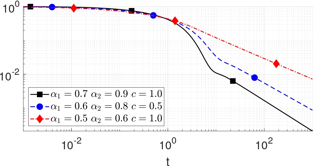
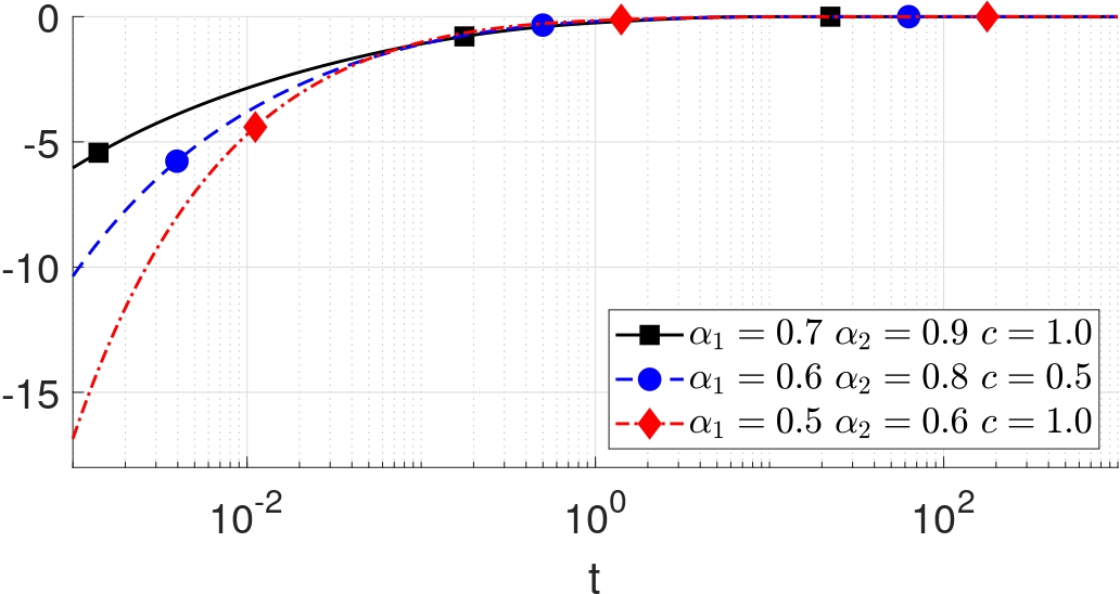
Figure 1. Solution $u_{A}(t)$ (left plot), and its first-order derivative $u^{\prime}_{A}(t)$ (right plot), of the variable-order relaxation equation with $\alpha(t)=\alpha_{1}+(\alpha_{1}-\alpha_{2})\mathrm{e}^{-ct}$ and different parameters $\alpha_{1}$, $\alpha_{2}$ and $c$.

3.2. Exponential transition with return

A further transition, recently introduced in [5], is obtained by means of the function

(3.4) $$\alpha(t)=\alpha_{1}+(\alpha_{2}-\alpha_{1})\frac{\mathrm{e}^{-c_{1}t}-\mathrm{e}^{-c_{2}t}}{F_{c}(c_{2}-c_{1})},\quad\alpha_{1},\alpha_{2}\in(0,1),\quad c_{1},c_{2}>0.$$

Unlike the previous one, this function describes an order transition which starts from $\alpha_{1}$, increases (or decreases) to $\alpha_{2}$ and hence returns back to $\alpha_{1}$ as $t\rightarrow\infty$. Thus, in this case, the condition (3.2) holds for $\alpha^{\prime}=\alpha^{\prime\prime}=\alpha_{1}.$ The constant $F_{c}$ is chosen so that $\alpha(t)$ has maximum or minimum value $\alpha_{2}$, and hence it is given by

$$F_{c}=\frac{1}{c_{2}-c_{1}}\left[\Bigl{(}\frac{c_{1}}{c_{2}}\Bigr{)}^{\frac{c_{1}}{c_{2}-c_{1}}}-\Bigl{(}\frac{c_{1}}{c_{2}}\Bigr{)}^{\frac{c_{2}}{c_{2}-c_{1}}}\right],$$

and $\alpha_{2}$ is achieved at time $t=(c_{2}-c_{1})^{-1}\log c_{2}/c_{1}$. Moreover, it is simple to evaluate

$$A(s)=\frac{1}{s}\alpha_{1}+\frac{\alpha_{2}-\alpha_{1}}{F_{c}(s+c_{1})(s+c_{2})},\quad s^{sA(s)}=s^{\alpha_{1}}s^{\frac{s(\alpha_{2}-\alpha_{1})}{F_{c}(s+c_{1})(s+c_{2})}}.$$

Also in this case a precise characterization of the whole set of possible choices for $\alpha_{1}$, $\alpha_{2}$, $c_{1}$ and $c_{2}$ to ensure that $s^{sA(s)}$ is Bernstein does not seem possible. Again, numerical inversion of the LT is used to guarantee that there exist some sets of parameters such that the solution to the renewal equation (2.6) has the properties required in Theorem 3.1. From Figure 2 we observe the non-negativity of these solutions (left plot) and its non-increasing character expressed as non-positivity of the corresponding first-order derivatives (right plot).

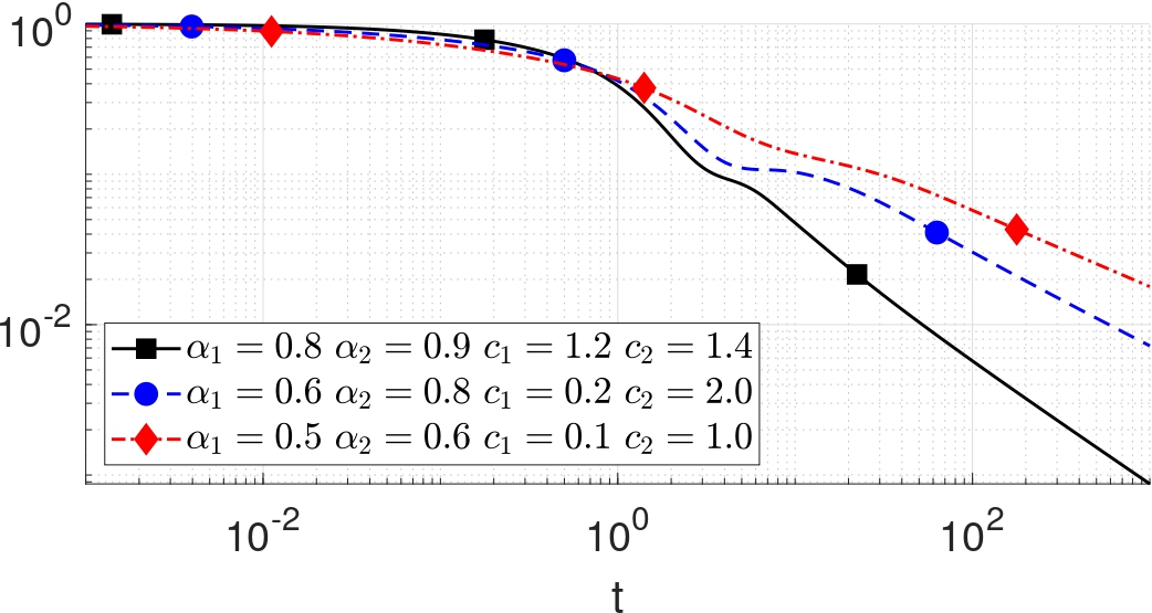
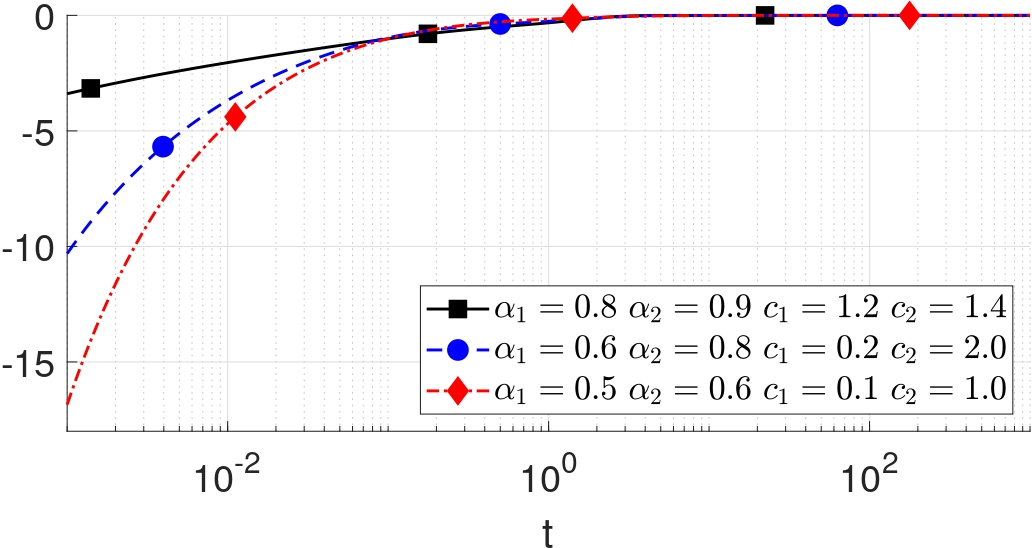
Figure 2. Solution $u_{A}(t)$ (left plot), and its first-order derivative $u^{\prime}_{A}(t)$ (right plot), of the variable-order relaxation equation with $\alpha(t)=\alpha_{1}+(\alpha_{2}-\alpha_{1})\frac{\mathrm{e}^{-c_{1}t}-\mathrm{e}^{-c_{2}t}}{F_{c}(c_{2}-c_{1})}$ and different parameters $\alpha_{1}$, $\alpha_{2}$, $c_{1}$ and $c_{2}$.

4. The variable-order fractional renewal process

By resorting to the results obtained so far, we can define a renewal process by assuming that its interarrival times have tail distribution function equal to the solution of the relaxation equation (2.6).

Definition 4.1.

Let $N_{A}(t):=\left\{N_{A}(t)\right\}_{t\geq 0}$ be a renewal process with interarrival times $Z_{A,j}$, $j=1,2,...,$ independent and identically distributed with $P(Z_{A}>t)=u_{A}(t)$, where $u_{A}(t)$, $t\geq 0,$ coincides with the solution of (2.6).

The density function of $Z_{A,j}$ can be written in Laplace domain as

(4.1) $$\widetilde{f}_{Z_{A}}(s\}=\frac{\lambda}{\lambda+s^{sA(s)}},$$

while the LT of the $k$-th renewal time density reads

(4.2) $$\widetilde{f}_{T_{k}^{A}}(s)=\frac{\lambda^{k}}{\left(\lambda+s^{sA(s)}\right)^{k}},\qquad k=1,2,...,$$

where $T_{k}^{A}:=\sum_{j=1}^{k}Z_{A,j}.$ Thus the probability mass function (in Laplace domain) of $N_{A}$ can be obtained as follows

$$\widetilde{p}_{k}^{A}(s) := \mathcal{L}\left\{P\left(N_{A}(t)=k\right);s\right\}=\frac{\lambda^{k}}{s\left(\lambda+s^{sA(s)}\right)^{k}}-\frac{\lambda^{k+1}}{s\left(\lambda+s^{sA(s)}\right)^{k+1}}$$

$$= \frac{\lambda^{k}s^{sA(s)-1}}{\left(\lambda+s^{sA(s)}\right)^{k+1}},\qquad k=0,1,...,\;t\geq 0,$$

and $p_{k}^{A}(t)$ satisfies the following Cauchy problem

(4.4) $$D_{t}^{\alpha(t)}p_{k}(t)=-\lambda(p_{k}(t)-p_{k-1}(t)),\qquad p_{k}(0)=1_{\{0\}}(k),$$

for $k=0,1,2,...$ and$\;t\geq 0.$

It is proved in [4], by some counterexamples, that, in the variable order case, $\widetilde{\phi}_{A}(s)$ is not in general a Stieltjes function; as a consequence, also the function (3.1) is not Stieltjes. Thus, in our case, the solution of the relaxation equations $u_{A}(t)$ can not be expressed as integral of the exponential tail distribution (as in (2.8)) and a time-change representation (analogue to that given in (2.11)) does not hold for the renewal process $N_{A}.$

We give in Figure 3 the probability mass function $p^{A}_{k}(t)$, for small values of $k$, in the first explanatory special case introduced above (i.e. for $\alpha(t)=\alpha_{1}+(\alpha_{1}-\alpha_{2})\mathrm{e}^{-ct}$). One can observe that, with the exponential transition from $\alpha_{1}$ to $\alpha_{2}$, the variable-order probability mass functions have a similar behavior to the corresponding functions of order $\alpha_{1}$ for $t\to 0^{+}$ and of order $\alpha_{2}$ as $t\to\infty$.

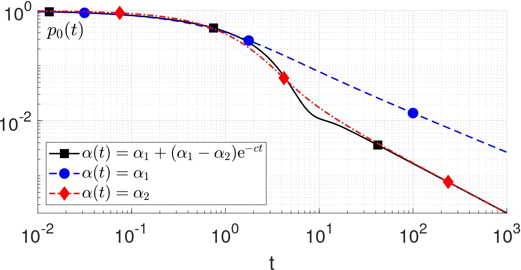
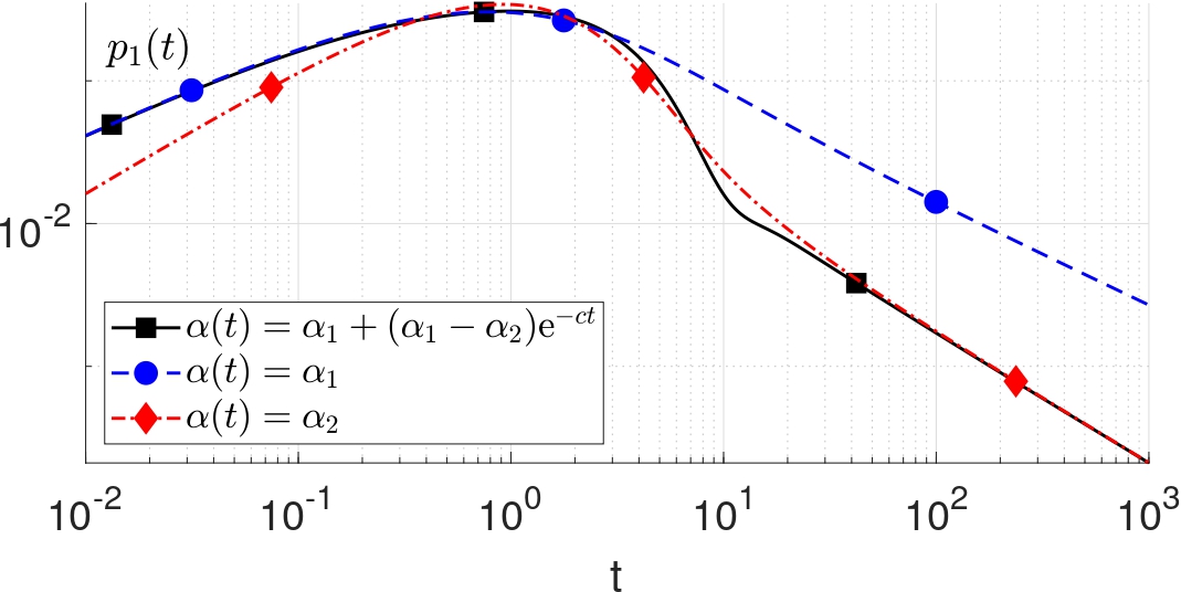
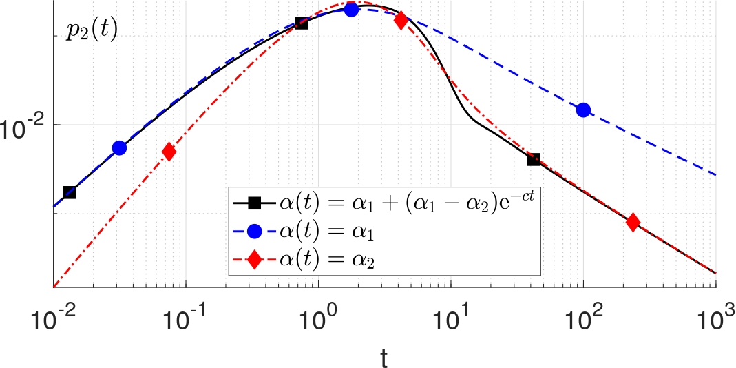
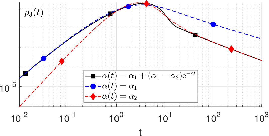
Figure 3. Comparison of probability mass functions $p^{A}_{k}(t)$, $k=0,1,2,3$ between exponential variable-order $\alpha(t)=\alpha_{1}+(\alpha_{1}-\alpha_{2})\mathrm{e}^{-ct}$ and constant orders $\alpha_{1}$ and $\alpha_{2}$ (here $\alpha_{1}=0.7$, $\alpha_{2}=0.9$ and $c=1.0$).

On the other side, as one can observe from Figure 4, with the variable-order transition (3.4), the behavior is similar to the behavior of the probability mass functions of constant order $\alpha_{1}$ both as $t\to 0^{+}$ and as $t\to\infty$, while the behavior with the constant order $\alpha_{2}$ is replicated just on short intervals at medium times.

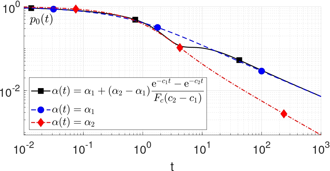
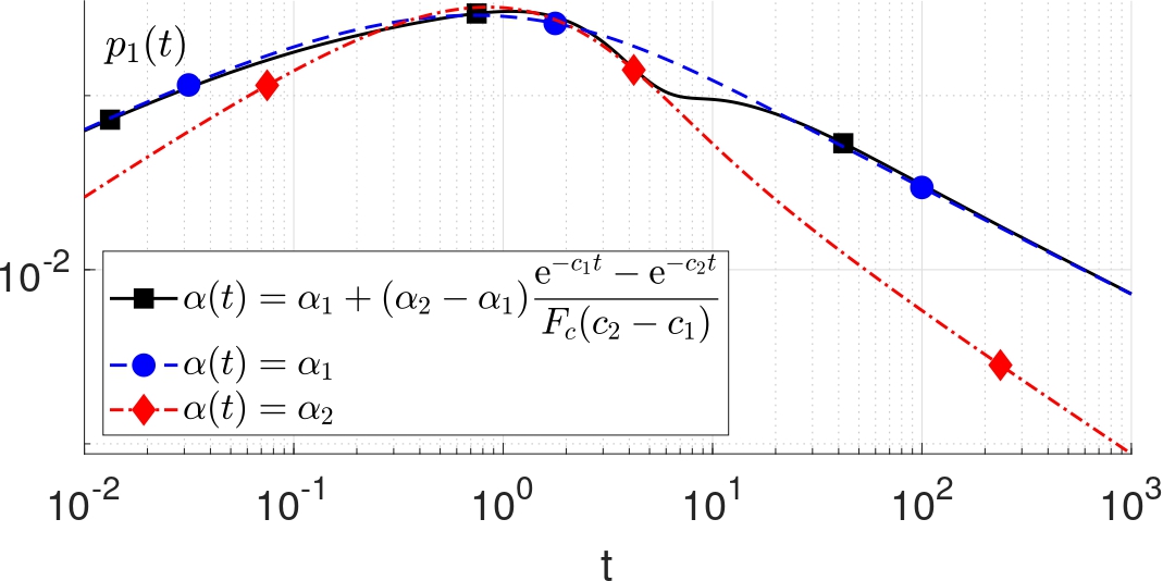
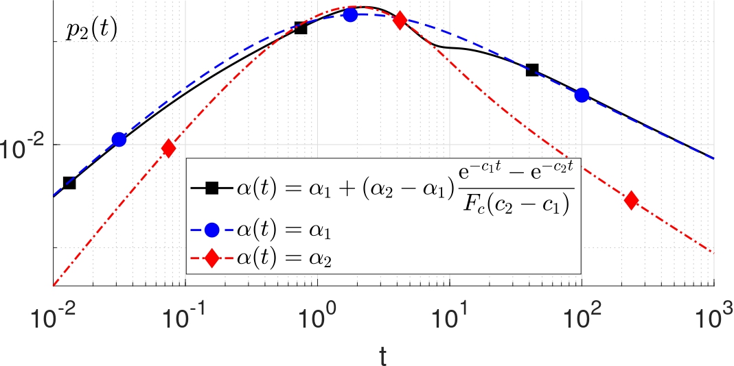
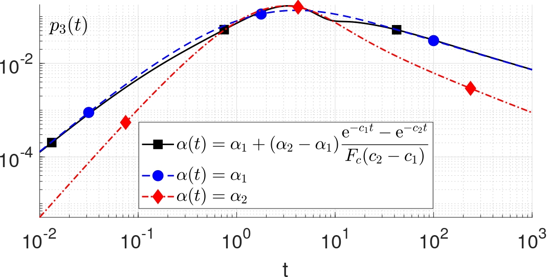
Figure 4. Comparison of probability mass functions $p^{A}_{k}(t)$, $k=0,1,2,3$ between exponential variable-order $\alpha(t)=\alpha_{1}+(\alpha_{2}-\alpha_{1})\frac{\mathrm{e}^{-c_{1}t}-\mathrm{e}^{-c_{2}t}}{F_{c}(c_{2}-c_{1})}$ and constant order $\alpha_{1}$ (here $\alpha_{1}=0.6$, $\alpha_{2}=0.8$, $c_{1}=0.2$ and $c_{2}=2.0$).

We are now interested in the properties of the above defined process, starting from its factorial moments and the moments of its interarrival times.

Theorem 4.1.

The $r$-th factorial moment of $N_{A}$, $r\in\mathbb{N}$, has LT

(4.5) $$\mathcal{L}\left\{\mathbb{E}\left[N_{A}(t)\cdot\cdot\cdot(N_{A}(t)-r+1)\right];s\right\}=\frac{r!\lambda^{r}}{s^{rsA(s)+1}}.$$

Moreover, the $r$-th moment of its interarrival time $Z_{A}$ is infinite for any $r\in\mathbb{N}$.

Proof.

In order to prove formula (4.5) we derive the expression of the probability generating function of $N_{A}$ (in the Laplace domain), as follows, for $|u|<1$,

$$\widetilde{G}_{N_{A}}(u;s) := \mathcal{L}\left\{G_{N_{A}}(u;t);s\right\}=\sum_{k=0}^{\infty}u^{k}\widetilde{p}^{A}_{k}(s)$$

$$= [\text{by (\ref{pk})}]$$

$$= \frac{s^{sA(s)-1}}{\lambda+s^{sA(s)}}\sum_{k=0}^{\infty}\frac{(u\lambda)^{k}}{\left(\lambda+s^{sA(s)}\right)^{k}}$$

$$= \frac{s^{sA(s)-1}}{\lambda(1-u)+s^{sA(s)}},$$

Now, by taking the $r$-th order derivative of (4), for $u=1$, formula (4.5) easily follows.

As far as the moments of the interarrival times are concerned, we first prove that the expected value is infinite: indeed we have that

$$\mathbb{E}Z_{A} = \lim_{s\rightarrow 0^{+}}\int_{0}^{+\infty}e^{-st}P(Z_{A}>t)dt$$

$$= \lim_{s\rightarrow 0^{+}}\frac{s^{sA(s)-1}}{\lambda+s^{sA(s)}}=+\infty,$$

where the interchange between limit and integral is justified by the monotone convergence theorem. The last step follows by applying the conditions (3.2), which imply (3.3), and by considering that $\alpha^{\prime},\alpha^{\prime\prime}\in(0,1),$ so that $\lim_{s\rightarrow 0^{+}}s^{sA(s)-1}=+\infty$ and $\lim_{s\rightarrow 0^{+}}s^{sA(s)}=0$. Finally, by applying the Holder’s inequality to $Z_{A}$ and taking into account that it is a non-negative random variable, we can conclude that the moments are infinite for any $r=2,3,..$ ∎

In order to evaluate the autocovariance of $N_{A}$ (at least in the Laplace domain), we recall the following result by [26], which holds for any renewal process $M(t):=\left\{M(t)\right\}_{t\geq 0}$ with density function of the interarrival times $f(\cdot)$:

(4.7) $$\int_{0}^{+\infty}\int_{0}^{+\infty}e^{-s_{1}t_{1}-s_{2}t_{2}}\mathbb{E}M(t_{1})M(t_{2})dt_{1}dt_{2}=\frac{\left[1-\widetilde{f}(s_{1})\widetilde{f}(s_{2})\right]\widetilde{f}(s_{1}+s_{2})}{s_{1}s_{2}\left[1-\widetilde{f}(s_{1})\right]\left[1-\widetilde{f}(s_{2})\right]\left[1-\widetilde{f}(s_{1}+s_{2})\right]},$$

for $s_{1},s_{2}\geq 0.$ By considering (4.1), we immediately obtain from (4.7) that

$$\int_{0}^{+\infty}\int_{0}^{+\infty}e^{-s_{1}t_{1}-s_{2}t_{2}}Cov\left[N_{A}(t_{1}),N_{A}(t_{2})\right]dt_{1}dt_{2}$$

$$= \frac{\lambda^{2}\left[s_{1}^{s_{1}A(s_{1})}+s_{2}^{s_{2}A(s_{2})}-(s_{1}+s_{2})^{(s_{1}+s_{2})A((s_{1}+s_{2}))}\right]+\lambda s_{1}^{s_{1}A(s_{1})}s_{2}^{s_{2}A(s_{2})}}{s_{1}^{s_{1}A(s_{1})+1}s_{2}^{s_{2}A(s_{2})+1}(s_{1}+s_{2})^{(s_{1}+s_{2})A((s_{1}+s_{2}))}.}$$

It is possible to check that, in the fixed order case, i.e. for $sA(s)=\alpha,$ formula (4) reduces to the LT of the well-known autocovariance of the fractional Poisson process, which is equal to:

(4.9) $$Cov\left[N_{\alpha}(t_{1}),N_{\alpha}(t_{2})\right]=\frac{\lambda\left(t_{1}\wedge t_{2}\right)^{\alpha}}{\Gamma(1+\alpha)}+\frac{\lambda^{2}}{\Gamma(1+\alpha)^{2}}\left[\alpha\left(t_{1}\wedge t_{2}\right)^{2\alpha}B(\alpha,\alpha+1)+F(\alpha;t_{1}\wedge t_{2};t_{1}\vee t_{2})\right],$$

where $B(\alpha,\beta):=\int_{0}^{1}x^{\alpha-1}(1-x)^{\beta-1}dx$ is the Beta function, $\alpha,\beta\geq 0$, $F(\alpha;x;y):=\alpha y^{2\alpha}B(\alpha,\alpha+1;x/y)-x^{\alpha}y^{\alpha}$ and $B(\alpha,\beta;x):=\int_{0}^{x}y^{\alpha-1}(1-y)^{\beta-1}dy$ is the incomplete Beta function, for $x\in(0,1]$, $\alpha,\beta\geq 0$ (see [12]). By taking the double LT of (4.9) we have that

$$\int_{0}^{+\infty}\int_{0}^{+\infty}e^{-s_{1}t_{1}-s_{2}t_{2}}Cov\left[N_{\alpha}(t_{1}),N_{\alpha}(t_{2})\right]dt_{1}dt_{2}$$

$$= \frac{\lambda}{\Gamma(1+\alpha)}\int_{0}^{+\infty}e^{-s_{2}t_{2}}\left[\int_{0}^{t_{2}}e^{-s_{1}t_{1}}t_{1}^{\alpha}dt_{1}+\int_{t_{2}}^{+\infty}e^{-s_{1}t_{1}}t_{1}^{\alpha}dt_{1}\right]dt_{2}+$$

$$+\frac{\lambda^{2}}{\Gamma(1+2\alpha)}\int_{0}^{+\infty}e^{-s_{2}t_{2}}\left[\int_{0}^{t_{2}}e^{-s_{1}t_{1}}t_{1}^{2\alpha}dt_{1}+t_{2}^{2\alpha}\int_{t_{2}}^{+\infty}e^{-s_{1}t_{1}}dt_{1}\right]dt_{2}+$$

$$+\frac{\lambda^{2}\alpha}{\Gamma(1+\alpha)^{2}}\int_{0}^{+\infty}e^{-s_{2}t_{2}}t_{2}^{2\alpha}dt_{2}\int_{0}^{t_{2}}e^{-s_{1}t_{1}}dt_{1}\int_{0}^{t_{1}/t_{2}}z^{\alpha-1}(1-z)^{\alpha}dz+$$

$$+\frac{\lambda^{2}\alpha}{\Gamma(1+\alpha)^{2}}\int_{0}^{+\infty}e^{-s_{2}t_{2}}dt_{2}\int_{t_{2}}^{+\infty}e^{-s_{1}t_{1}}t_{1}^{2\alpha}dt_{1}\int_{0}^{t_{2}/t_{1}}z^{\alpha-1}(1-z)^{\alpha}dz+$$

$$-\frac{\lambda^{2}}{\Gamma(1+\alpha)^{2}}\int_{0}^{+\infty}e^{-s_{2}t_{2}}t_{2}^{\alpha}dt_{2}\int_{0}^{+\infty}e^{-s_{1}t_{1}}t_{1}^{\alpha}dt_{1}$$

$$=: I_{s_{1},s_{2}}^{I}+I_{s_{1},s_{2}}^{II}+I_{s_{1},s_{2}}^{III}+I_{s_{2},s_{1}}^{III}+I_{s_{1},s_{2}}^{IV}.$$

By some calculations we easily obtain the following results:

(4.10) $$I_{s_{1},s_{2}}^{I} = \frac{\lambda}{s_{1}s_{2}(s_{1}+s_{2})^{\alpha}}$$

(4.11) $$I_{s_{1},s_{2}}^{II} = \frac{\lambda^{2}}{s_{1}s_{2}(s_{1}+s_{2})^{2\alpha}}$$

(4.12) $$I_{s_{1},s_{2}}^{IV} = \frac{\lambda^{2}}{s_{1}^{1+\alpha}+s_{2}^{1+\alpha}},$$

while for the terms of the third type, we must take into account the following formula (see (1.6.15) together with (1.6.14) and (1.9.3) in [8]):

$$\int_{0}^{1}e^{zt}t^{a-1}(1-t)^{c-a-1}dt=\Gamma(c-a)E_{1,c}^{a}(z),$$

for $0<\operatorname{Re}(a)<\operatorname{Re}(c)$, where $E_{\alpha,\beta}^{\gamma}\left(\cdot\right)$ is the Mittag-Leffler function with three parameters (also called Prabhakar function), for any $x\in\mathbb{C}$,

$$E_{\alpha,\beta}^{\gamma}\left(x\right):=\sum_{j=0}^{\infty}\frac{(\gamma)_{j}x^{j}}{j!\Gamma(\alpha j+\beta)},\qquad\alpha,\beta,\gamma\in\mathbb{C}\text{, }\operatorname{Re}(\alpha)>0,$$

for $(\gamma)_{j}:=\Gamma(\gamma+j)/\Gamma(\gamma).$ We also recall the well-known formula (see [8], p.47)

(4.13) $$\mathcal{L}\left\{t^{\beta-1}E_{\alpha,\beta}^{\gamma}(at^{\alpha});s\right\}=\frac{s^{\alpha\gamma-\beta}}{\left(s^{\alpha}-a\right)^{\gamma}},\qquad|as^{-\alpha}|<1.$$

Thus we can write

$$I_{s_{1},s_{2}}^{III} = \frac{\lambda^{2}\alpha}{\Gamma(1+\alpha)^{2}}\int_{0}^{+\infty}e^{-s_{2}t_{2}}t_{2}^{2\alpha}dt_{2}\int_{0}^{1}z^{\alpha-1}(1-z)^{\alpha}dz\int_{zt_{2}}^{t_{2}}e^{-s_{1}t_{1}}dt_{1}$$

$$= \frac{\lambda^{2}\alpha}{\Gamma(1+\alpha)^{2}}\frac{1}{s_{1}}\int_{0}^{+\infty}e^{-s_{2}t_{2}}t_{2}^{2\alpha}dt_{2}\int_{0}^{1}z^{\alpha-1}(1-z)^{\alpha}\left[e^{-s_{1}t_{2}z}-e^{-s_{1}t_{2}}\right]dz$$

$$= \frac{\lambda^{2}}{s_{1}}\left[\int_{0}^{+\infty}e^{-s_{2}t_{2}}t_{2}^{2\alpha}E_{1,2\alpha+1}^{\alpha}\left(-s_{1}t_{2}\right)dt_{2}-\frac{1}{(s_{1}+s_{2})^{2\alpha+1}}\right]$$

$$= \frac{\lambda^{2}}{s_{1}}\left[\frac{1}{s_{2}^{\alpha+1}(s_{1}+s_{2})^{\alpha}}-\frac{1}{(s_{1}+s_{2})^{2\alpha+1}}\right]$$

and, analogously, for $I_{s_{2},s_{1}}^{III}.$ In view of (4.10), (4.11), (4.12) and (4), we obtain that

$$\int_{0}^{+\infty}\int_{0}^{+\infty}e^{-s_{1}t_{1}-s_{2}t_{2}}Cov\left[N_{\alpha}(t_{1}),N_{\alpha}(t_{2})\right]dt_{1}dt_{2}=\frac{\lambda s_{1}^{\alpha}s_{2}^{\alpha}+\lambda^{2}\left[s_{1}^{\alpha}+s_{2}^{\alpha}-(s_{1}+s_{2})^{\alpha}\right]}{s_{1}^{\alpha+1}s_{2}^{\alpha+1}(s_{1}+s_{2})^{\alpha}},$$

which coincides with (4), when $sA(s)=\alpha.$

5. The related continuous-time random walk and its limiting process

Based on the previous results, we consider the continuous-time random walk (hereafter CTRW) defined by means of the counting process $N_{A}$: let $X_{i},i=1,2,...$ be real, independent random variables with common density function $f_{X}(\cdot)$ and let us denote $\widehat{g}(\kappa):=\int_{\mathbb{R}}e^{i\kappa x}g(x)dx$, for $\kappa\in\mathbb{R}$ and for a function $g:\mathbb{R}\rightarrow\mathbb{R}$, for which the integral converges. We define, for any $t\geq 0,$ the CTRW with driving counting process $N_{A}$ and jumps $X_{i}$ (under the assumption that $N_{A}$ and $X_{i}$ are independent each other) as

(5.1) $$Y_{A}(t):=\sum_{i=1}^{N_{A}(t)}X_{i},$$

and denote its density as $f_{Y_{A}}(y,t):=P(Y_{A}(t)\in dy)/dy.$ Then it is well-known that the LT of the characteristic function of $Y_{A}(t)$ reads, for any $t\geq 0,$

$$\mathcal{L}\left\{\widehat{f}_{Y_{A}}(\kappa,t);s\right\}=\frac{1-\widetilde{f}_{Z_{A}}(s)}{s\left[1-\widetilde{f}_{Z_{A}}(s)\widehat{f}_{X}(\kappa)\right]},\qquad s\geq 0,\text{ }\kappa\in\mathbb{R},$$

where $\widetilde{f}_{Z_{A}}(s)$ is the LT of the interarrivals’ density. By considering (4.1), we get

(5.2) $$\mathcal{L}\left\{\widehat{f}_{Y_{A}}(\kappa,t);s\right\}=\frac{s^{sA(s)-1}}{s^{sA(s)}+\lambda[1-\widehat{f}_{X}(\kappa)]}.$$

We are now able to study the limiting behavior of the CTRW under an appropriate rescaling. To this aim, we recall the definition of the time-space fractional diffusion $Y_{\alpha,\beta}^{\vartheta}(t),t\geq 0$ as the process whose density is the Green function of the following equation, for $\alpha\in(0,1]$, $\beta\in(0,2],$ $|\vartheta|=\min\{\beta,2-\beta\},$

(5.3) $${}^{C}D_{t}^{\alpha}u(x,t)=\mathcal{D}_{x}^{\beta,\vartheta}u(x,t),\qquad x\in\mathbb{R},\;t\geq 0,$$

where $\mathcal{D}_{x}^{\beta,\vartheta}$ is the Riesz-Feller fractional derivative with Fourier transform

$$\widehat{\mathcal{D}_{x}^{\beta,\vartheta}u}(\kappa)=-\psi_{\beta,\vartheta}(\kappa)\widehat{u}(\kappa),\qquad\kappa\in\mathbb{R},$$

and $\psi_{\beta,\vartheta}(\kappa):=|\kappa|^{\beta}e^{i\,sign(\kappa)\vartheta\pi/2}$ (see [15], for details).

We also recall the definition of a stable random variable $\mathcal{S}_{\beta}$ with stability index $\beta\in(0,2]$ and symmetry parameter $|\vartheta|=\min\{\beta,2-\beta\}$, which is defined by the following characteristic function

$$\mathbb{E}e^{i\kappa\mathcal{S}_{\beta}}=e^{-\psi_{\beta,\vartheta}(\kappa)}=e^{-|\kappa|^{\beta}e^{i\,sign(\kappa)\vartheta\pi/2}}.$$

We will consider hereafter $\mathcal{S}_{\beta}$ in the symmetric case, i.e. we assume that $\vartheta=0.$

We recall that a (centered) random variable $X$ is said to be ”in the domain of attraction of $\mathcal{S}_{\beta}$” (and we write $X\in DoA(\mathcal{S}_{\beta})$), if the following convergence in law (by the extended central limit theorem) holds for the rescaled sum of independent copies $X_{i},$ $i=1,2,...,$

(5.4) $$a_{n}\sum_{i=1}^{n}X_{i}\Longrightarrow\mathcal{S}_{\beta},$$

where $\left\{a_{n}\right\}_{n\geq 1}$ is a sequence such that $\lim_{n\rightarrow+\infty}a_{n}=0.$

Theorem 5.1.

Let $N_{A}^{(c)}(t)$, $t\geq 0,$ be the renewal process with (rescaled) $k$-th renewal time $T_{k}^{A,c}:=c^{-1}\sum_{j=1}^{k}Z_{A,j}$, where $Z_{A,j}$ are i.i.d. random variables with density (4.2), for $c>0$ and let $X_{i}^{(c)}$ be i.i.d. centered r.v.’s with density $f_{X^{(c)}}$, (with scale parameter $1/c$), such that $\widehat{f}_{X^{(c)}}(\kappa/c)\simeq 1-(|\kappa|/c)^{\beta}$, for $c\rightarrow+\infty.\$Then the following convergence of the one-dimensional distribution holds, as $c\rightarrow+\infty,$

(5.5) $$c^{-\alpha^{\prime\prime}/\beta}\sum_{i=1}^{N_{A}^{(c)}(t)}X_{i}^{(c)}\Longrightarrow Y_{\alpha^{\prime\prime},\beta}(t),\qquad t>0,$$

where $Y_{\alpha^{\prime\prime},\beta}(t)$ is the space-time fractional diffusion process, whose transition density satisfies equation (5.3), with time-derivative of order $\alpha^{\prime\prime}=lim_{t\rightarrow+\infty}\alpha(t),$ $\beta\in(0,2]$ and $\vartheta=0.$

Proof.

The characteristic function of (5.5) can be written, for any $t\geq 0,$ as

$$\mathbb{E}e^{i\kappa c^{-\alpha^{\prime\prime}/\beta}\sum_{i=1}^{N_{A}^{(c)}(t)}X_{i}^{(c)}}=\sum_{n=0}^{\infty}p_{n}^{A,c}(t)\left[\widehat{f}_{X^{(c)}}(\kappa c^{-\alpha^{\prime\prime}/\beta})\right]^{n},$$

where $p_{n}^{A,c}(t):=P\left(N_{A}^{(c)}(t)=n\right),$ $t\geq 0,$ $n=0,1,....$ We note that

$$p_{n}^{A,c}(t) = P(T_{n}^{A,c}<t)-P(T_{n+1}^{A,c}<t)$$

$$= P\left(\sum_{j=1}^{n}Z_{A,j}<ct\right)-P\left(\sum_{j=1}^{n+1}Z_{A,j}<ct\right)=p_{n}^{A}(ct),$$

so that, by (4), we have

$$\int_{0}^{+\infty}e^{-st}p_{n}^{A,c}(t)dt=\frac{1}{c}\frac{\lambda^{n}(s/c)^{\frac{s}{c}A(s/c)-1}}{\left(\lambda+(s/c)^{\frac{s}{c}A(s/c)}\right)^{n+1}}$$

and

$$\mathcal{L}\left\{\mathbb{E}e^{i\kappa c^{-\alpha^{\prime\prime}/\beta}\sum_{i=1}^{N_{A}^{(c)}(t)}X_{i}^{(c)}};s\right\} = \frac{1}{c}\frac{(s/c)^{\frac{s}{c}A(s/c)-1}}{(s/c)^{\frac{s}{c}A(s/c)}+\lambda[1-\widehat{f}_{X}(\kappa c^{-\alpha^{\prime\prime}/\beta})]}$$

$$= \frac{s^{\frac{s}{c}A(s/c)-1}}{s^{\frac{s}{c}A(s/c)}+\lambda[1-\widehat{f}_{X}(\kappa c^{-\alpha^{\prime\prime}/\beta})]c^{\frac{s}{c}A(s/c)}}.$$

We observe that $lim_{r\rightarrow 0^{+}}srA(sr)=\alpha^{\prime\prime}$ and thus $lim_{c\rightarrow+\infty}s^{\frac{s}{c}A(s/c)}=s^{\alpha^{\prime\prime}},$ by (3.3). Moreover, by assumption, $\widehat{f}_{X}(\kappa c^{-\alpha^{\prime\prime}/\beta})\simeq 1-c^{-\alpha^{\prime\prime}}|\kappa|^{\beta}$, for $c\rightarrow+\infty.$ As a consequence, we have

$$\lim_{c\rightarrow+\infty}\mathcal{L}\left\{\mathbb{E}e^{i\kappa c^{-\alpha^{\prime\prime}/\beta}\sum_{i=1}^{N_{A}^{(c)}(t)}X_{i}^{(c)}};s\right\}=\frac{s^{\alpha^{\prime\prime}}-1}{s^{\alpha^{\prime\prime}}+\lambda|\kappa|^{\beta}}$$

and, inverting the LT by means of (4.13), we can write

(5.6) $$\lim_{c\rightarrow+\infty}\mathbb{E}e^{i\kappa c^{-\alpha^{\prime\prime}/\beta}\sum_{i=1}^{N_{A}^{(c)}(t)}X_{i}^{(c)}}=E_{\alpha^{\prime\prime}}(-\lambda t^{\alpha^{\prime\prime}}|\kappa|^{\beta}),$$

for any fixed $t\geq 0$. Formula (5.6) coincides with the Fourier transform of the Green function of (5.3) (see [15], for details). ∎

The previous result reduces, in the fixed order case, to Theorem IV.2 in [22], if $\alpha(t)=\alpha^{\prime\prime}$, for any $t$; thus we can conclude that, in the limit, the influence of the initial parameter $\alpha^{\prime}$ vanishes.

Let us now denote by $\overset{M_{1}}{\Longrightarrow}$ the convergence in the $M_{1}$ topology in the Skorokhod space $D([0,T))$, for $T>0$ (see [27] and [21] for details on the convergence in the $M_{1}$ topology).

Theorem 5.2.

Let $Y_{A}^{(c)}(t):=\sum_{i=1}^{N_{A}(ct)}X_{i}^{(c)}$, then under the assumptions of Theorem 5.1

$$\left\{c^{-\alpha^{\prime\prime}/\beta}Y_{A}^{(c)}(t)\right\}_{t\geq 0}\overset{M_{1}}{\Longrightarrow}\left\{Y_{\alpha^{\prime\prime},\beta}(t)\right\}_{t\geq 0},\qquad c\rightarrow+\infty,$$

on $D([0,+\infty)).$

Proof.

We start by proving that, for the r.v.’s $X_{i}^{(c)},$ the convergence in (5.4) holds for $a_{c}=c^{-1/\beta}$ since

(5.7) $$\mathbb{E}e^{i\kappa c^{-1/\beta}\sum_{i=1}^{c}X_{i}^{(c)}}=\left(\widehat{f}_{X^{(c)}}\left(\kappa c^{-1/\beta}\right)\right)^{c}\simeq\left(1-|\kappa|^{\beta}c^{-1}\right)^{c},\qquad c\rightarrow+\infty.$$

Thus $X^{(c)}\in DoA(\mathcal{S}_{\beta})$, $c\rightarrow+\infty.$ Under the assumptions on $\alpha(\cdot)$ and $A(\cdot)$ given in Theorem 3.1, we can easily see that $T_{\left\lfloor ct\right\rfloor}^{A}:=\sum_{j=1}^{\left\lfloor ct\right\rfloor}Z_{A,j}$ behaves asymptotically, for $c\rightarrow+\infty,$ as in the special case (of the fractional Poisson process) where $Z_{A}$ is distributed as $\mathcal{A}_{\alpha}(Z),$ where $\mathcal{A}_{\alpha}(t),$ $t\geq 0,$ is an $\alpha$-stable subordinator (with $\alpha=\alpha^{\prime\prime})$ and $Z$ is an independent, exponential r.v. with parameter $\lambda.$ Indeed, since, by (3.3), $\lim_{s\rightarrow 0^{+}}sA(s)=\alpha^{\prime\prime},$ we can derive that

$$\mathcal{L}\left\{P\left(Z_{A}>t\right);s\right\}\sim\frac{s^{\alpha^{\prime\prime}-1}}{s^{\alpha^{\prime\prime}}+\lambda},\qquad s\rightarrow 0^{+},$$

by considering (3.1). Thus the following convergence holds $\{T_{\left\lfloor ct\right\rfloor}^{A}\}_{t\geq 0}\overset{J_{1}}{\Rightarrow}\{\mathcal{A}_{\alpha^{\prime\prime}}(t)\}_{t\geq 0},$ as $c\rightarrow+\infty,$ in $D([0,+\infty))$ (see [21], p.100).

By the independence of $Z_{A,j}$ and $X_{j}^{(c)},$ for any $j=1,2...$ and by the functional central limit theorem, we have that

$$\left\{c^{-1/\beta}\sum_{j=1}^{[ct]}X_{j}^{(c)},c^{-\alpha^{\prime\prime}}N_{A}(ct)\right\}_{t\geq 0}\overset{J_{1}}{\Longrightarrow}\left\{\mathcal{S}_{\beta}(t),\mathcal{L}_{\alpha^{\prime\prime}}(t)\right\}_{t\geq 0},\qquad c\rightarrow+\infty,$$

in the $J_{1}$ topology on $D([0,+\infty)).$ Therefore, by the above mentioned Theorem 2.1 in [20], the following convergence holds

$$\left\{c^{-\alpha^{\prime\prime}/\beta}Y_{A}^{(c)}(t)\right\}_{t\geq 0}\overset{M_{1}}{\Longrightarrow}\left\{\mathcal{S}_{\beta}(\mathcal{L}_{\alpha^{\prime\prime}}(t))\right\}_{t\geq 0},\qquad c\rightarrow+\infty,$$

which gives the desired result, by considering the well-known equality in distribution $\mathcal{S}_{\beta}(\mathcal{L}_{\alpha^{\prime\prime}}(t))\overset{d}{=}Y_{\alpha^{\prime\prime},\beta}(t)$ (see [15]). ∎

Remark 5.1.

As a special case of the previous result, when $\beta=2$ and $\lambda=1/2$, we obtain the convergence of the process $Y_{A}^{(c)},$ for $c\rightarrow\infty,$ to the so-called generalized grey Brownian motion $\mathcal{B}_{\alpha}(t),t\geq 0,$ (with $\alpha=\alpha^{\prime\prime}),$ which can be defined by means of its characteristic function $\mathbb{E}e^{i\kappa\mathcal{B}_{\alpha}(t)}=E_{\alpha}(-t^{\alpha}\kappa^{2}/2)$ (see [17] and [18]).

References

[1] Beghin, L., Orsingher, E. Fractional Poisson processes and
related planar motions. Electron.J.Probab. 2009; 14, 1790–1827.
[2] Beghin L., Random-time processes governed by differential equations
of fractional distributed order, Chaos, Solitons and Fractals, 2012; 45, 1314–1327.
[3] Feller W., An Introduction Probability Theory and its
Applications, vol.2 (2nd ed.), Wiley, New York, (1971).
[4] Garrappa R., Giusti A., Mainardi F., Variable-order fractional
calculus: A change of perspective, Commun Nonlinear Sci. Numer. Simulat. 2021; 102, 105904.
[5] Garrappa R., Giusti A., Mainardi F., Variable-Order
Fractional Calculus: from Old to New Approaches, IEEE Proceedings,
2022.
[6] Gorenflo R., Kilbas A.A., Mainardi F., Rogosin S.V. Mittag-Leffler Functions, Related Topics and Applications. Springer-Verlag,
Berlin Heidelberg; 2014.
[8] A.A.Kilbas, H.M.Srivastava, J.J.Trujillo, Theory and
Applications of Fractional Differential Equations, vol. 204, North-Holland
Mathematics Studies, Elsevier Science B.V., Amsterdam, 2006.
[9] Kochubei AN . General fractional calculus, evolution
equations, and renewal processes. Integr Equ Oper Theory, 2011; 71:
583–600.
[10] Kochubei AN . General fractional calculus. In: Handbook
of fractional calculus with applications. Vol. 1. Berlin: De Gruyter; 2019.
p. 111–26.
[11] Kochubei AN . Equations with general fractional time
derivatives-Cauchy problem. In: Handbook of fractional calculus with
applications. Vol. 2. De Gruyter, Berlin; 2019. p. 223–34.
[12] Leonenko N., Meerschaert M.M., Schilling R.L., Sikorskii A.
Correlation structure of time-changed Lévy processes. Communications in Applied and Industrial Mathematics, 2014; 6; 1; 1-22.
[13] Le Page WR . Complex variables and the Laplace transform
for engineers. Dover Publications, Inc, New York; 1980.
[14] Luchko Y . Operational calculus for the general fractional
derivative and its applications. Fract Calculus Appl Anal, 2021; 24:
338–75.
[15] Mainardi F., Applications of integral transforms in
fractional diffusion processes, Integral Transforms and Special
Functions. 2004; 15; 6; 477-484.
[16] Mainardi F., Gorenflo R., Scalas E., A fractional
generalization of the Poisson processes, Vietnam Journal of Mathematics, 2004; 32; 53-64.
[17] A.Mura, F.Mainardi, A class of self-similar stochastic
processes with stationary increments to model anomalous diffusion in
physics, Integral Transform and Special Functions, 20, Nos. 3-4,
(2009), 185-198.
[18] A.Mura, G.Pagnini, Characterizations and simulations of a
class of stochastic processes to model anomalous diffusion, Journal of
Physics A: Math. Theor., 41 (2008), 285003, 22 p.
[19] Meerschaert, M. M., Nane, E., Vellaisamy, P. The fractional
Poisson process and the inverse stable subordinator. Electron. J.
Probab. 2011; 16:1600–1620.
[20] Meerschaert, M.M., Scheffler, H.P.: Triangular array limits
for continuous time random walks. Stoch. Proc. Applic. 118, 1606-1633 (2008).
[21] Meerschaert, M.M., Sikorskii, A., Stochastic Models for
Fractional Calculus. De Gruyter, Berlin-Boston (2012)
[22] Scalas, E., A class of CTRWs: compound fractional Poisson
processes. Fractional Dynamics. 2011; 353-374.
[23] Scarpi G. Sulla possibilità di un modello reologico
intermedio di tipo evolutivo. Atti Accad Naz Lincei Rend Cl Sci Fis
Mat Nat (8) 1972;52:912–17 (1973).
[24] R.L.Schilling, R.Song, Z.Vondracek, Bernstein Functions:
Theory and Applications, 37, De Gruyter Studies in Mathematics Series,
Berlin, 2010.