Asymptotic analysis and efficient random sampling of directed ordered acyclic graphs

Abstract

Directed acyclic graphs (DAGs) are directed graphs in which there is no path from a vertex to itself. DAGs are an omnipresent data structure in computer science and the problem of counting the DAGs of given number of vertices and to sample them uniformly at random has been solved respectively in the 70’s and the 00’s. In this paper, we propose to explore a new variation of this model where DAGs are endowed with an independent ordering of the out-edges of each vertex, thus allowing to model a wide range of existing data structures.

We provide efficient algorithms for sampling objects of this new class, both with or without control on the number of edges, and obtain an asymptotic equivalent of their number. We also show the applicability of our method by providing an effective algorithm for the random generation of classical labelled DAGs with a prescribed number of vertices and edges, based on a similar approach. This is the first known algorithm for sampling labelled DAGs with full control on the number of edges, and it meets a need in terms of applications, that had already been acknowledged in the literature.

1 Introduction

Directed Acyclic Graphs (DAGs for short) are directed graphs in which there is no directed path (sequence of incident edges) from a vertex to itself. They are an omnipresent data structure in various areas of computer science and mathematics. In concurrency theory for instance, scheduling problems usually define a partial order on a number of tasks, which is naturally encoded as DAG via its Hasse diagram [Cor+10, CEH19]. DAGs also appear as the result of the compression of some tree-like structures such as XML documents [Bou+15]. In functional programming in particular, this happens at the memory layout level of persistent tree-like values, where the term “hash-consing” has been coined to refer to this compression [Got74]. Computer algebra systems also make use of this idea to store their symbolic expression [Ers58]. Finally, complex histories, such as those used in version control systems (see Git for instance [Gei+18, p. 17]) or genealogy “trees” are DAGs as well.

Two kinds of DAGs have receive a particular interest: labelled DAGs and unlabelled DAGs. The most obvious one the labelled model, in which one has a set $V$ of distinguishable vertices (often $\llbracket 1;n\rrbracket$) connected by a set of edges $E\subseteq V\times V$. The term labelled is used because the vertices can be distinguished here, they can be assigned labels. On the other hand, unlabelled DAGs are the quotient set obtained by considering labelled DAGs up to relabelling, that is to say up to a permutation of their vertices (which is reflected on the edges). These two types of objects serve a different purpose, the former represents relations over a given set whereas the latter represents purely structural objects. From a combinatorial point of view, a crucial difference between the two models is that one has to deal with symmetries when enumerating unlabelled DAGs which makes the counting and sampling problem significantly more involved.

The problem of counting DAGs has been solved in early 70’s by Robinson [Rob70, Rob73, Rob77] and Stanley [Sta73] using different approaches. Robinson exhibits a recursive decompositions of labelled DAGs leading to a recurrence satisfied by the numbers $A_{n,k}$ of DAGs with $n$ vertices including $k$ sources (vertices without any incoming edge). Stanley on the other hand uses a generating function approach using identities of the chromatic polynomial. Robinson also solves the unlabelled case starting from the same ideas but using Burnside’s lemma and cycle index sums to account for the symmetries of these objects. He provides a first solution in [Rob70] and makes it more computationally tractable in [Rob77]. In the 90’s, Gessel uses a novel approach based on so-called graphical generating function in [Ges95, Ges96] to take into account more parameters and count DAGs by vertices and edges, but also sinks and sources.

From the point of view of uniform random generation, the recursive decomposition exhibited by Robinson in [Rob73] is interesting as it is amenable to the recursive method pioneered by Nijenhuis and Wilf in [NW78]. This yields a polynomial time algorithm for sampling uniform DAGs with $n$ vertices. The analysis of this algorithm has been done in [KM15] but it had been acknowledged earlier in [MDB01] although the article proposes an alternative solution. Both [KM15] and [MDB01] also offer a Markov chain approach to the random sampling problem. Unfortunately, to our knowledge, no efficient uniform random generator of unlabelled has been found yet. Moreover, unlike in the labelled case, the method derived by Robinson to exhibit the number of unlabelled DAGs cannot be easily leveraged into a random sampler as they make extensive use of Burnside’s lemma. Another interesting question is that of controlling the number of edges in random those samplers. Indeed, sampling a uniform DAG with a prescribed number of vertices and edges cannot be achieved using the Markov chain approach as it constrains the chain too much, and the formulas of Gessel are not amenable to this either. In [KM15, § 7], the authors provide an interesting discussion on which kind of restrictions can be made on DAGs with the Markov chain approach. They discuss in particular the case of bounding the number of edges and highlight the benefits the having a precise combinatorial enumeration compared to Markov chains.

In the present paper, we propose to study an alternative model of DAGs, which we call Directed Ordered Acyclic Graphs (DOAGs), and which are enriched with additional structure on the edges. More precisely, a DOAG in an unlabelled DAG where (1) set of outgoing edges of each vertex is totally ordered, (2) the sources are totally ordered as well, and (3) graphs are constrained to have only one sink. This local ordering of the sources allows to capture more precisely the structure of existing mathematical objects. For instance, the compressed formulas and tree-like structures mentioned earlier (see [Ers58, Got74]) indeed present with an ordering as soon as the underlying tree representation is ordered. This is the case for most trees used in computer science (e.g. red-black trees, B-trees, etc.) and for all formulas involving non-commutative operators. We present here several results regarding DOAGs, as well as an extension of our method to classical labelled DAGs.

As a first step of our analysis, we describe a recursive decomposition scheme that allows us to study DOAGs using tools from enumerative combinatorics. This allows us to obtain a recurrence formula for counting them, as well as a polynomial-time uniform random sampler, based on the recursive method from [NW78], giving full control over their number of vertices and edges. Our decomposition is based on a “vertex-by-vertex” approach, that is we remove one vertex at a time and we are able to describe exactly what amount of information is necessary to reconstruct the graph. This differs from the approach of Robinson to study DAGs, where here removes all the sources of a DAG at once instead. Although this is a minor difference, our approach allows us to easily account for the number of edges of the graph, which is why our random sampler is able to target DOAGs with a specific number of vertices. In terms of application, this means that we are able to efficiently sample DOAGs of low density. A second by-product of our approach is that it makes straightforward to bound the out-degree of each vertex, thus allowing to sample DOAGs of low degree as well.

In order to show the applicability of our method, we devise a similar decomposition scheme for counting labelled DAGs with only one sink. This allows us to transfer our results on DOAGs in the context of labelled DAGs. More precisely, we present a new recurrence formula for counting labelled DAGs with one sink by number of vertices, edges and sources and which differ from the formula of Gessel [Ges96] counting the same objects. Our approach allows us to obtain an efficient uniform random sampler of labelled DAGs (with one sink) with a prescribed number of vertices and edges. Here again, in addition to giving control over the number of edges of the produced objects, our approach can also be adapted to bound the out-degree of their vertices. To our knowledge, this is the first such sampler.

Finally, in a second part of our study of DOAGs, we focus on their asymptotic behaviour and get a first result in this direction. We consider the number $D_{n}$ of DOAGs with $n$ vertices, one source, and any number of edges, and we manage to exhibit an asymptotic equivalent of an uncommon kind:

$$D_{n}\sim c\cdot n^{-1/2}\cdot e^{n-1}\prod_{k=1}^{n-1}k!\quad\text{for some constant~{}$c>0$.}$$

In the process of proving this equivalent, we state an upper bound on $D_{n}$ by exhibiting a super-set of the set of DOAGs of size $n$, expressed in terms of simple combinatorial objects: variations. This upper-bound is close enough to $D_{n}$ so that we can leverage it into an efficient uniform rejection sampler of DOAGs with $n$ vertices and any number of edges. Combined with an efficient anticipated rejection procedure, allowing to reject invalid objects as soon as possible, this lead us to an optimal uniform sampler of DOAGs of size $n$.

Outline of the paper

In Section 2, we start by introducing the class of Directed Ordered Acyclic Graphs and their recursive enumeration and describe a recursive decomposition scheme allowing to count them. We quickly go over a counting algorithm implementing the recurrence. In Section 3, we describe and analyse an effective uniform random sampler of DOAGs giving full control over the number of edges, vertices, and sources based on the recursive decomposition. Then, in Section 4, we present a bijection between DOAGs and class of integer matrices. This bijection proves to be a key element in understanding the structure of DOAGs in the two following sections. In Section 5, we present a first asymptotic result: we give an asymptotic equivalent of the number of DOAGs of size $n$ with any number of sources and edges. We also state some simple structural properties of those DOAGs. In light of the matrix encoding and these asymptotic results, we design an optimal uniform random sampler of DOAGs with a given number of vertices (but no constraint on the number of edges), that is described in Section 6. Finally in Section 7, we open the way for further research directions regarding the classical model of labelled DAGs. We show that our approach, when applied to labelled DAGs, yields a constructive counting formula for them, that is amenable to efficient uniform random generation with full control on the number of edges.

An implementation of all the algorithms presented in this paper is available at https://github.com/Kerl13/randdag. This paper extends [GPV21] with a new result on the asymptotics of DOAGs, with an optimal uniform random sampler for the case when the number of edges is not prescribed, and covers a larger class of DOAGs and DAGs by drooping a constraint on the number of sinks.

2 Definition and recursive decomposition

We introduce a model of directed acyclic graphs called “Directed Ordered Acyclic Graphs” (or DOAGs) which is similar to the classical model of unlabelled DAGs but where, in addition, we have a total order on the outgoing edges of each vertex.

Definition 1 (Directed Ordered Graph).

A directed ordered graph is a triple $(V,E,{(\prec_{v})}_{v\,\in V\cup\{\emptyset\}})$ where:

• $V$ is a finite set of vertices;

• $E\subset V\times V$ is a set of edges;

• for all $v\in V$, $\prec_{v}$ is a total order over the set of outgoing edges of $v$;

• and $\prec_{\emptyset}$ is a total order over the set of sources of the graph, that is the vertices without any incoming edge.

Two such graphs are considered to be equal if there exists a bijection between their respective sets of vertices that preserves both the edges and the order relations $\prec_{v}$ and $\prec_{\emptyset}$.

Definition 2 (Directed Ordered Acyclic Graph).

A directed ordered acyclic graph (or DOAG for short) is a directed ordered graph $(V,E,{(\prec_{v})}_{v\,\in V\cup\{\emptyset\}})$ such that $(V,E)$, seen as a directed graph, is acyclic.

We study this class as a whole, however, some sub-classes are also of special interest, in particular for the purpose of modelling compacted data structures. Tree structures representing real data, such as XML documents for instance, are rooted trees. When these trees are compacted, the presence of a root translates into a unique source in the resulting DOAG. Similarly, DOAGs with a single sink will arise naturally when compacting trees which bear a single type of leaves. For this reason, we will also discuss how to approach the sub-classes of DOAGs with a single source and/or a single sink in this document. As an example, the first line of Figure 1 depicts all the DOAGs with exactly $3$ edges and $4$ vertices (among which exactly $2$ are sources). On the second line, we also listed all DOAGs with exactly one sink, one source, and up to $4$ edges.

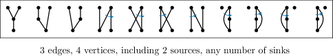
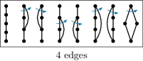
Figure 1: On the first line: all DOAGs with exactly $3$ edges and $4$ vertices, among which exactly $2$ are sources. On the second line: all DOAGs with exactly $1$ source, $1$ sink, and up to $4$ edges. All edges are implicitly oriented from top to bottom. The leftmost source is the smallest one in every picture. The order of the outgoing edges of each vertex is indicated by the thinner blue arrows (always from left to right here).

2.1 Recursive decomposition

We describe a canonical way to recursively decompose a DOAG into smaller structures. The idea is to remove vertices one by one in a deterministic order, starting from the smallest source (with respect to their ordering $\prec_{\emptyset}$). Formally, we define a decomposition step as a bijection between the set of DOAGs with at least two vertices and the set of DOAGs given with some extra information. Let $D$ be a DOAG with at least $2$ vertices and consider the new graph $D^{\prime}$ obtained from $D$ by removing its smallest source $v$ and its outgoing edges. We also need to specify the ordering of the sources of $D^{\prime}$. We consider the ordering where the new sources of $D^{\prime}$ (those that have been uncovered by removing $v$) are considered to be in the same order (with respect to each other) as they appear as children of $v$ and all larger than the other sources. The additional information necessary to reconstruct $D$ from $D^{\prime}$ is the following:

1. the number $s\geq 0$ of sources of $D^{\prime}$ which have been uncovered by removing $v$;

2. the (possibly empty) set $I$ of internal (non-sources) vertices of $D^{\prime}$ such that there was an edge in $D$ from $v$ to them;

3. the function $f:I\to\llbracket 1;s+|I|\rrbracket$ identifying the positions, in the list of outgoing edges of $v$, of the edges pointing to an element of $I$.

In fact, this decomposition describes a bijection between DOAGs with at least $2$ vertex and quadruples of the form $(D^{\prime},s,I,f)$ where $D^{\prime}$ is a DOAG with $k^{\prime}$ sources, $I$ is a subset of its internal vertices, $0\leq s\leq k^{\prime}$ is a non-negative integer, and $f:I\to\llbracket 1;s+|I|\rrbracket$ is an injective function. Indeed, the inverse transformation is as follows. Create a new source $v$ with $s+|I|$ outgoing edges such that the $i$-th of these edges is connected to $f^{-1}(i)$ when $i\in f(I)$ and is connected to one of the $s$ largest sources of $D^{\prime}$ otherwise. The $s$ largest sources of $D^{\prime}$ must be connected to the new source exactly once and in the same order as they appear in the list of sources of $D^{\prime}$. Note that the order in which the vertices are removed when iterating this process corresponds to a BFS-based topological sort of the graph. Fig. 2 pictures the first $3$ decomposition steps of an example DOAG.

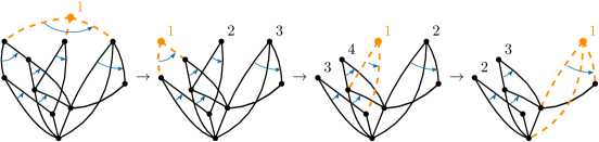
Figure 2: Recursive decomposition of a DOAG by removing sources one by one in a breadth first search (BFS) fashion. The edges are implicitly oriented from top to bottom and the order of the outgoing edges of each vertex is indicated by the thinner blue arrows (always from left to right here). The integer labels at each stage indicate the ordering of the sources.

This decomposition can be used to establish a recursive formula for counting DOAGs, which is given below. Let $D_{n,m,k}$ denote the number of DOAGs with $n$ vertices, $m$ edges and $k$ sources, then we have:

$$D_{1,m,k} =\boldsymbol{1}_{\{m=0\,\land\,k=1\}}$$ (1)

$$D_{n,m,k} =0 \text{when}~{}k\leq 0$$

$$D_{n,m,k} =\sum_{p=0}^{n-k}\sum_{i=0}^{p}D_{n-1,m-p,k-1+p-i}\binom{n-k-p+i}{i}\binom{p}{i}i!$$ otherwise,

where $p=s+i$ corresponds the out-degree of the smallest source, the term $\binom{n-k-p+i}{i}=\binom{n-k-s}{i}$ accounts for the choice of the set $I$ and the term $\binom{p}{i}i{!}$ accounts for the number of injective functions $f:I\to\llbracket 1;p\rrbracket$. The upper bound on $p$ in the sum is justified by the following combinatorial arguments. Since $p$ is the out-degree of the smallest source, it is upper bounded by the number of vertices it might have an outgoing edge to, that is the number $(n-k)$ of non-source vertices of the graph.

2.1.1 Special sub-classes based on out-degree constraints

Since $p=i+s$ is the out-degree of the removed source in the above summation, it is easy to adapt this sequence for counting DOAGs with constraints on the out-degree of the vertices. For instance, DOAGs with only one sink are obtained by ensuring that every vertices has at least out-degree one. In other words, let the summation start at $p=1$. Note that restricting DOAGs to have only one single sink or one single source ensures that they remain connected, however not all connected DOAGs are obtained this way. As another example, DOAGs with out-degree bounded by some constant $d$ are obtained by letting $p$ range from $0$ to $\min(n-k,d)$.

The general principle is that the DOAGs whose vertices’ out-degrees are constrained to belong to a given set $\mathcal{P}$, are enumerated by the following recursive formula.

$$D^{\mathcal{P}}_{1,m,k} =\boldsymbol{1}_{\{m=0\,\land\,k=1\}}$$ (2)

$$D^{\mathcal{P}}_{n,m,k} =0 \text{when}~{}k\leq 0$$

$$D^{\mathcal{P}}_{n,m,k} =\sum_{p\in\mathcal{P}}\sum_{i=0}^{p}D^{\mathcal{P}}_{n-1,m-p,k-1+p-i}\binom{n-k-p+i}{i}\binom{p}{i}i!$$ otherwise,

The first values of the sequence $D_{n,m}=\sum_{k}D_{n,m,k}$ counting DOAGs by number of vertices and edges only are given in Table 1. Table 2 gives the first values of $D^{\mathcal{P}}_{n}=\sum_{m,k}D^{\mathcal{P}}_{n,m,k}$ for some choices of $\mathcal{P}$. None of these sequences seem to appear in the online encyclopedia of integer sequences (OEIS) yet.

Table 1: Number of DOAGs with $n$ vertices and $m$ edges for small values of $n$ and $m$.

$n$	$D_{n}$	$D_{n,m}=\sum_{k}D_{n,m,k}$ for $m=0,1,2,3,\ldots$
$1$	$1$	$1$
$2$	$2$	$1,1$
$3$	$8$	$1,2,3,2$
$4$	$95$	$1,3,8,17,27,27,12$
$5$	$4858$	$1,4,15,48,139,349,718,1136,1272,888,288$
$6$	$1336729$	$1$, $5$, $24$, $100$, $391$, $1434$, $4868$, $14940$, $40261$, $92493$, $175738$, $266898$, $310096$, $258120$, $136800$, $34560$

Table 2: Number of DOAGs with $n$ vertices and a constrained set of allowed degrees.

Restrictions	sequence
$\mathcal{P}=\mathbb{N}$	$1$, $2$, $8$, $95$, $4858$, $1336729$, $2307648716$, $28633470321822$, $2891082832793961795$, $2658573971407114263085356$, $24663703371794815015576773905384$, $\ldots$
$\mathcal{P}=\mathbb{N}$, $k=1$	$1$, $1$, $4$, $57$, $3399$, $1026944$, $1875577035$, $24136664716539$, $2499751751065862022$, $2342183655157963146881571$, $22043872387559770578846044961204$, $\ldots$
$\mathcal{P}=\mathbb{N}^{\star}$, $k=1$	$1$, $1$, $3$, $37$, $2103$, $627460$, $1142948173$, $14701782996075$, $1522511169925136833$, $1426529804350999351686869$, $13426022673540053054145359653988$, $\ldots$
$\mathcal{P}=\{0,1,2\}$, $k=1$	$1$, $1$, $4$, $23$, $191$, $2106$, $29294$, $495475$, $9915483$, $229898277$, $6074257926$, $180460867600$, $5962588299084$, $\ldots$

2.2 Computational aspects of the counting problem

In order to implement a random sampler for DOAGs, we will have to pre-compute the values of $D_{n,m,k}$ for all $n,m$, and $k$ up to a given bound. This can be achieved easily using equation 1 and a dynamic programming approach. We do not give the algorithm here as it is a straightforward implementation of the above formula. But in this section we give some details on its computational aspects. First, in Lemma 1 we characterise the indices $n,m,k$ such that $D_{n,m,k}>0$. This can be used to avoid unnecessary recursive calls and to choose a memory-efficient data-structure for storing the results. Then in Theorem 1 we give the complexity of the counting procedure in terms of bitwise operations.

Lemma 1.

For $n>1$, we have $D_{n,m,k}\neq 0$ if and only if $1\leq k\leq n$ and $n-k\leq m\leq\binom{n}{2}-\binom{k}{2}$.

Proof.

There is always at least one source in a DOAG, hence $1\leq k\leq n$ is a necessary condition for $D_{n,m,k}$ to be non-zero. Now let $n$ and $k$ be such that $1\leq k\leq n$ and consider $n$ vertices labelled from $1$ to $n$. The maximum possible number of edges in a DOAG with $k$ sources is obtained by putting an edge from vertex $i$ to vertex $j$ if and only if $i<j$ and $j>k$ as pictured below.

This corresponds to $\binom{n}{2}-\binom{k}{2}$ edges since there are $\binom{n}{2}$ pairs $(i,j)$ such that $i<j$ and $\binom{k}{2}$ pairs $(i,j)$ such that $i<j\leq k$. Furthermore, it is possible to remove any number of edges from this maximal case while keeping at least one edge to each vertices $i>k$. This accounts for $(n-k)$ mandatory edges. ∎

In Theorem 1 we get a straightforward upper bound on the number of arithmetic operations necessary to compute all the $D_{n,m,k}$ up to certain bounds. As it is usual in combinatorial enumeration, there is a hidden cost factor in the size of the numbers at stake: the more they grow the more costly arithmetic operations become. To account for this cost we also give an upper bound on the bit-size of all numbers being multiplied.

Theorem 1.

Let $N,M>0$ be two integers. Computing $D_{n,m,k}$ for all $n\leq N$, $m\leq M$ and all possible $k$ can be done with $O(N^{4}M)$ multiplications of integers of size at most $O(\max(M,N)\ln N)$.

The first part of Theorem 1 is straightforward but we need a bound on the value of $D_{n,m,k}$ for the second part, which is the purpose of Lemma 2.

Lemma 2.

For all $n,m,k$, we have $\displaystyle{D_{n,m,k}\leq\binom{\binom{n}{2}-\binom{k}{2}}{m}\cdot m!}$

Proof.

This upper bound is based on two combinatorial arguments. Consider a sequence of $n$ vertices obtained by decomposing a DOAG $D$ with $k$ sources and $m$ edges. The first $k$ vertices of this sequence thus correspond to the $k$ sources of $D$.

First, the set of edges of $D$ is a subset of size $m$ of the set of all pairs of vertices that are not made of two sources. Note that not all such subsets form a valid DAG however. Hence, the number of ways to choose the $m$ edges of $D$ is bounded above by $\binom{\binom{n}{2}-\binom{k}{2}}{m}$. Second, the number of ways to order the outgoing edges of all the vertices is bounded by $d_{1}!d_{2}!\cdots d_{n}{!}$ where $d_{j}$ denotes the out-degree of the $i$-th vertex. Finally, this product is bounded by $m{!}$, which corresponds to the case where all the $d_{j}$ but one are equal to $0$ and the remaining one is equal to $m$. ∎

This bound on the number of DOAGs is rough but it is precise enough to get an estimation of the bit-size of these numbers.

Corollary 1.

There exists a constant $c>0$ such that for all $n,m,k$ we have $\log_{2}(D_{n,m,k})\leq c\cdot m\cdot\log_{2}n$.

Proof.

Let $L=\binom{n}{2}-\binom{k}{2}$. By Lemma 2, we have that:

$$D_{n,m,k}\leq\frac{L(L-1)(L-2)\cdots(L-m+1)}{m!}\cdot m!\leq L^{m}.$$

Hence, $\log_{2}(D_{n,m,k})\leq m\log_{2}(L)$. Moreover $\log_{2}(L)\leq\log_{2}(n^{2})=2\log_{2}(n)$, which allows to conclude. ∎

We now have enough information to prove Theorem 1.

Proof of Theorem 1..

Since $D_{n,m,k}=0$ for $k>n$, we need to compute $O(N^{2}M)$ numbers. Moreover, computing each $D_{n,m,k}$ requires to compute a sum of at most $n^{2}$ terms, each of which is the product of a number of bit-length $O(m\ln n)$ with a coefficient of the form $C(j,p,i)=\binom{j+i}{i}\binom{p}{i}i{!}$ (for some $j,p,i\leq n$) of bit-length $O(n\ln n)$. Overall this accounts for $O(N^{4}M)$ multiplications of bit-complexity $\mathcal{M}({M\ln N})$ since $m=O(n^{2})$.

There remains to measure the cost of computing the coefficients $C(j,p,i)$. They can be obtained at a small amortized cost using the relation $C(j,p,i)=C(j,p,i-1)\cdot\frac{(j+i)(p-i+1)}{i}$ (for all $1<i\leq p$) to get the value of the coefficient at $i$ from its value at $i-1$ when summing the terms of 1 for increasing values of $i$. Clearly, the cost of multiplying numbers of bit-length $n\ln n$ and $\ln n$ is bounded by $\mathcal{M}({n\ln n})$ and therefore $\mathcal{M}({N\ln N})$.

Combining the these two arguments, we get $O(\mathcal{M}({\max(N,M)\ln N}))$ for the cost of each multiplication. ∎

3 Recursive sampling algorithm

In this section we describe a uniform random sampler of DOAGs based on the recursive decomposition given in the previous section. Our algorithm is based on the so-called “recursive method” from [NW78] in the way we select the parameters of the sub-structures. However, unlike what we would expect in the systematised framework from [FZV94], the substructures are not independent. Once the sub-DOAG $D^{\prime}$ accounted for by $D_{n-1,m-p,k-1+p-i}$ has been selected, the set $I$ and the injective function $f:I\to\llbracket 1;|I|+s\rrbracket$ accounted for by $\binom{n-k-p+i}{i}\binom{p}{i}i{!}$ cannot be sampled independently from $D^{\prime}$.

Our random sampler is given in Algorithm 1. We first give a high-level description of the algorithm here for the sake of readability. Implementation considerations are discussed below, and in particular in Algorithm 2 we give a fast algorithm for the generation of the outgoing edges of the new source at each step of the global random sampling procedure.

Algorithm 1 Recursive uniform sampler of DOAGs

1:Three integers $(n,m,k)$ such that $D_{n,m,k}>0$

2:A uniform random DOAG with $n$ vertices (including $k$ sources) and $m$ edges

3:function UnifDOAG($n,m,k$)

4:     if $n=1$ then generate the (unique) DOAG with $1$ vertices

5:     else

6:         pick $(p,i)$ with probability $\displaystyle{D_{n-1,m-p,k-1+p-i}\binom{n-k-p+i}{i}\binom{p}{i}i{!}}/{D_{n,m,k}}$

7:         $D^{\prime}\leftarrow\text{{UnifDOAG}($n-1,m-p,k-1+p-i$)}$

8:         $I\leftarrow$ a uniform subset of size $i$ of the inner vertices of $D^{\prime}$

9:         $I^{\prime}\leftarrow$ a uniform permutation of $I$

10:         $E\leftarrow$ a uniform shuffling of $I^{\prime}$ with the $s=p-i$ largest sources of $D^{\prime}$

11:         return the DOAG obtained by adding a new source to $D^{\prime}$ with $E$ as its list of outgoing edges      

The pick instruction at line 6 implements the “recursive method” scheme: pick the parameters of the sub-structures using the pre-computed counting information. The standard way to implement this is to draw a uniform random integer $r$ from the interval $[0;D_{n,m,k}-1]$ and then start to compute the sum of general term terms $D_{n-1,m-p,k-1+p-i}\binom{n-k-p+i}{i}\binom{p}{i}i{!}$ (in any order independent of $r$) until the sum is greater than $r$. The indices $p$ and $i$ of the last term of the sum are the ones to pick. Independently of the summation order, this procedure has complexity $O(n^{2})$ in the worst case in terms of multiplications of big integers. An interesting order of summation is the one where the pairs $(p,i)$ are taken in lexicographic order. In this case the complexity of the pick function can be expressed in terms of the result of the drawing as $O(p^{2})$, which is more informative about the cost of sampling the whole DOAG since $p$ is the out-degree of the new source. We consider that this order is used here.

Once we have sampled the sub-DOAG $D^{\prime}$, sampling $I$ is straightforward and the injective function $f$ is obtained as a permutation of $I$ (thus deciding of the order of the elements of $I$ as children of the new vertex) shuffled with the largest $(p-i)$ sources of $D^{\prime}$. The correctness and complexity of this procedure in terms of integer multiplications are stated in Theorem 2.

Theorem 2.

Algorithm 1 computes a uniform random DOAG with $n$ vertices (among which $k$ are sources) and $m$ edges by performing $O\left(\sum_{v}d_{v}^{2}\right)$ multiplications where $v$ ranges over the vertices of the resulting graph and $d_{v}$ is the out-degree of $v$.

Proof.

The complexity result is a straightforward consequence of the above discussion. Uniformity is proved by induction. Let $D$ be a DOAG of parameters $(n,m,k)$ and let $(D^{\prime},s,I,f)$ denote the result of one decomposition step of $D$. Then the probability that $D$ is returned by $\textsc{UnifDOAG}(n,m,k)$ is

$$\mathbb{P}[D]=\mathbb{P}[(p,i)]\cdot\mathbb{P}[D^{\prime}|p,i]\cdot\mathbb{P}[I|D^{\prime},i]\cdot\mathbb{P}[f|I,p,i]$$

where, by induction we have $\mathbb{P}[D^{\prime}|p,i]=1/D_{n-1,m-p,k-1+p-i}$ and by definition:

$$\mathbb{P}[(p,i)] =D_{n-1,m-p,k-1+p-i}\binom{n-k-p+i}{i}\binom{p}{i}i{!}/D_{n,m,k}$$

$$\mathbb{P}[I|D^{\prime},i] ={\binom{n-k-p+i}{i}}^{-1}$$

$$\mathbb{P}[f|I,p,i] ={\left(i!\binom{p}{i}\right)}^{-1}.$$

In the end, we get that $\mathbb{P}[D^{\prime}]=1/D_{n,m,k}$. ∎

Note that the sum $\sum_{v}d_{v}^{2}$ is of the order of $m^{2}$ in the worst case but can be significantly smaller if the out-degrees of the vertices are evenly distributed. In the best case we have $d_{v}\sim\frac{m}{n}$ for most of the vertices and as a consequence $\sum_{v}d_{v}^{2}\sim{m^{2}}/{n}$.

We have decomposed the generation of the new source into several steps in Algorithm 1 (lines 7 to 10) to make the role of each term in the counting formula apparent, and help stating the uniformity. However there is a faster way to implement this part of the Algorithm by sampling $I$ and its ordering together using a variant of the well-known Fisher–Yates algorithm (see [FY48]) using the property that the first $i$ terms of a uniform permutation form a uniform ordered subset of size $i$ of its elements. This is described in Algorithm 2 which can substitute lines 7 to 10 in Algorithm 1 in a practical implementation.

Algorithm 2 Optimised uniform sampler of new sources with given parameters

Two non-negative integers $i$ and $s$, an array $S$ of length $\ell_{S}\geq s$ vertices playing the role of sources and an array $T$ of length $\ell_{T}\geq i$ vertices playing the role of internal vertices.

An array $v$ of $i+s$ vertices, representing a new vertex with $s$ out-edges to the $s$ last elements of $S$ (appearing in the same order as in $S$) and $i$ edges to elements of $T$, chosen uniformly at random.

1:$i^{\prime}$ $\leftarrow$ $i$

2:$s^{\prime}$ $\leftarrow$ $s$

3:$v$ $\leftarrow$ new array of length $(i+s)$

4:for $j=0$ to $i-1$ do

5:     $r\leftarrow\text{{Unif}($\llbracket j;\ell_{T}-1\rrbracket$)}$

6:     $T[j]\leftrightarrow T[r]$

7:while $i^{\prime}+s^{\prime}>0$ do

8:     if Bern($i^{\prime}/(i^{\prime}+s^{\prime})$) then

9:         $v[i^{\prime}+s^{\prime}-1]\leftarrow T[i^{\prime}-1]$

10:         $i^{\prime}\leftarrow i^{\prime}-1$

11:     else

12:         $v[i^{\prime}+s^{\prime}-1]\leftarrow S[\ell_{S}-s+s^{\prime}-1]$

13:         $s^{\prime}\leftarrow s^{\prime}-1$      

The first loop of Algorithm 2 (at line 4) implements the Fisher–Yates algorithm with an early exit after $i$ iterations rather than $\ell_{T}$. After this, the first $i$ elements of $T$ represent the set $I$ and their ordering is uniform. The second loop (at line 7) implements the shuffling of $I$ with the last $s$ elements of $S$. We populate the array $v$ in reverse order so as to ensure that the elements coming from $S$ remain sorted.

This algorithm achieves linear complexity in $p=(i+s)$ in terms of memory accesses and number of calls to the random number generator, but needs to modify $T$ in place. Since $T$ represents the internal vertices of a DOAG, this means that we must choose a data structure for DOAGs that is not sensitive to the order of its internal vertices.

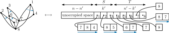
Figure 3: The memory layout used for storing DOAGs during the generation. The labels on the vertices of the DOAG on the left correspond to the order in which they are consumed by the decomposition. Each vertex on the left corresponds to a cell of the main array on the right. Each cell (except for the last one) has a pointer to an array of vertices representing its outgoing edges (here represented as integers for readability but stored as pointers in practice). For instance the cell labelled $1$ has three outgoing edges to the vertices labelled $7$, $8$ and $4$.

The idea is to represent a DOAG with $n$ vertices and $k$ sources as an array of vertices where the first $k$ elements are the sources, sorted in increasing order, and the other $n-k$ elements are the internal nodes stored in an unspecified order. Vertices are represented as pointers to arrays of vertices, the order of the elements encodes the order of the edges. One can then allocate a single array of size $n$ before the first call to the sampler and populate it from right to left in the recursive calls. The invariant is that, after each recursive call of the form $\textsc{UnifDOAG}(n^{\prime},m^{\prime},k^{\prime})$, the $n^{\prime}$ last elements of the array represent its resulting DOAG $D^{\prime}$ of size $n^{\prime}$. Algorithm 2 is then used by taking the $n^{\prime}-k^{\prime}$ last elements of the array as $T$ and the $k^{\prime}$ elements preceding them as $S$, without making any copy. Finally the newly generated source is stored at index $n-n^{\prime}$, just before the $n^{\prime}$ vertices representing $D^{\prime}$. The advantage of this memory layout is that after this point, the $s$ former sources that have been turned into internal nodes are already at the right place. The memory representation discussed above is pictured in Figure 3.

A remark on constrained out-degrees

Consider a set of allowed degrees $\mathcal{P}$ for the vertices. If the sequence $D_{n,m,k}^{\mathcal{P}}$ from equation (2) in Section 2.1.1 is used in place of $D_{n,m,k}$ in the algorithm, and without any further change, we obtain a uniform random sampler of DOAGs whose vertices have their out-degree in $\mathcal{P}$. The fact that only the sequence has to be changed and not the rest of the algorithm reflects the generality of the recursive method. A large DOAG of out-degree bounded by $10$, sampled using this algorithm, is shown in Figure 12 on page 12.

4 Matrix encoding

In this section, we introduce the notion of labelled transition matrices and give a bijection between DOAGs and these matrices, thus offering an alternative point of view on DOAGs. In the next two section, we then rely heavily on this encoding to prove an asymptotic equivalent for the number of DOAGs with $n$ vertices, and to design a efficient uniform random sampler for those DOAGs. We also recall the definition and basic properties of variations, which are an elementary combinatorial object playing a key role in our analysis.

4.1 The encoding

The decomposition scheme described in Section 2 corresponds to a traversal of the DOAG. This traversal induces a labelling of the vertices from $1$ to $n$, which allows us to associate the vertices of the graph to these integers in a canonical way. We then consider its transition matrix using these labels as indices. Usually, the transition matrix of a directed graph $D$ is defined as the matrix ${(a_{i,j})}_{1\leq i,j\leq n}$ such that $a_{i,j}$ is $1$ if there is an edge from vertex $i$ to vertex $j$ in $D$, and $0$ otherwise. This representation encodes the set of the edges of a DAG but not the edge ordering of DOAGs. In order to take this ordering into account, we use a slightly different encoding.

Definition 3 (Labelled transition matrix of a DOAG).

Let $D$ be a DOAG with $n$ vertices. We associate the vertices of $D$ to the integers from $1$ to $n$ corresponding to their order in the vertex-by-vertex decomposition. The labelled transition matrix of $D$ is the matrix ${(a_{i,j})}_{1\leq i,j\leq n}$ with integer coefficients such that $a_{i,j}=k>0$ if and only if there is an edge from vertex $i$ to vertex $j$ and this edge is the $k$-th outgoing edge of $i$. Otherwise $a_{i,j}=0$.

An example of a DOAG and its transition matrix are pictured in Figure 4. The thick lines are not part of the encoding and their meaning will be explained later. Let $\phi$ denote the function mapping a DOAG to its labelled transition matrix. This function is clearly injective as the edges of the graph can be recovered as the non-zero entries of the matrix, and the ordering of the outgoing edges of each vertex is given by the values of the corresponding entries in each row. Characterising the image of $\phi$ however requires more work.

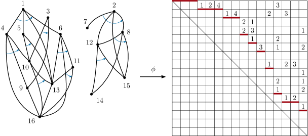
Figure 4: An example DOAG and its labelled transition matrix, the zeros are represented by the absence of a number.

We can make some observations. First, by definition of the traversal of the DOAG, the labelled transition matrix of a DOAG is strictly upper triangular. Indeed, since the decomposition algorithm removes one source at a time, the labelling it induces is a topological sorting of the graph. Moreover, since the non-zero entries of row $i$ encode the ordered set of outgoing edges of vertex $i$, these non-zero entries form a permutation

• a non-zero value cannot be repeated within a row;

• and if a row contains $d\geq 1$ non-zero entries, then these are the integers from $1$ to $d$, in any order.

Informally, these two properties ensure that a matrix encodes a labelled DOAG (a DOAG endowed with a labelling of its vertices) and that this labelling is a topological sorting of the graph. However, they are not enough to ensure that this topological sorting is precisely the one that is induced by the decomposition. The matrices satisfying these two properties will play an important role in the rest of the paper. We call them “variation matrices”.

Definition 4 (Variation).

A variation is a finite sequence of non-negative integers such that

1. each strictly positive number appears at most once;

2. if $0<i<j$ and $j$ appears in the sequence, then $i$ appears too.

The size of a variation is its length.

For instance, the sequence $(6,2,3,0,0,1,4,0,5)$ is a variation of size $9$ but the sequences $(1,0,3)$ and $(1,0,2,2)$ are not variations. Variations can also be defined as interleavings of a permutation with a sequence of zeros. One of the earliest references to these objects dates back to Izquierdo1659 in Izquierdo’s [Izq59] [Izq59, Disputatio 29]. They also appear in Stanley’s book as the second entry of his Twelvefold Way [Sta11, page 79], a collection of twelve basic but fundamental counting problems. Variations are relevant to our problem as they naturally appear as rows of the labelled transition matrices defined in this section. Some of their combinatorial properties will be exhibited in the next section.

Definition 5 (Variation matrix).

Let $n>0$ be a positive integer. A matrix of integers ${(a_{i,j})}_{1\leq i,j\leq n}$ is said to be a variation matrix if

• it is strictly upper triangular;

• for all $1\leq i\leq n-1$, the sub-row ${(a_{i,j})}_{i<j\leq n}$ is a variation (of size $n-i$).

Equivalently, a variation matrix can be seen as a sequence of variations $(v_{1},v_{2},\ldots,v_{n-1})$ where for all $1\leq i\leq n-1$, the variation $v_{i}$ has size $i$.

We have established that all labelled transition matrices of DOAGs are variation matrices. Note that the converse is not true. For instance, the matrix pictured in Figure 5 is a variation matrix of size $3$ that does not correspond to any DOAG. The property of this matrix which explains why it cannot be the image of a DOAG is pictured in red on the Figure, and will be explained in the rest of this section, in particular in Theorem 3.

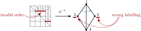
Figure 5: An example of a matrix of variations that cannot be obtained as a labelled transition matrix of a DOAG. The labelled DOAG that it encodes is not labelled according to the decomposition order.

We now characterise which of those variation matrices can be obtained as the labelled transition matrix of a DOAG. Consider such a matrix.

Note that in any column $j$, the non-zero entry with the highest index $i$ (that is in the lowest row on the picture with a non-zero element in column $j$) has a spacial role: it corresponds to the last edge pointing to vertex $j$ when decomposing the DOAG. These elements are underlined by a thick red line in Figure 4, and when a column has no non-zero entry at all, the top line is pictured in thick red instead. When several such cells occur on the same row $i$ in the matrix, they correspond to several sources that are discovered at the same time, upon removing vertex $i$ in the DOAG. Recall that the decomposition algorithm sorts the labels of these new sources by following the total order of the outgoing edges of vertex $i$. As a consequence, the entries above the thick red line have to be increasingly sorted (from left to right). For instance, observe that there are three consecutive underlined cells in the first row of the matrix in Figure 4. Indeed, when removing the first source of the DOAG on the left, we uncover three new sources which are respectively in first, second and fourth position in the outgoing edges order of the removed source.

Another important property is that if any underlined cells occur in a row of the matrix, these are always the first non-zero entries in that row. This is because, when the decomposition algorithm discovers new sources, it considers them to be larger than all the previously discovered sources. As a consequence, the vertices are processed (removed by the algorithm) in the same order as they become sources during the decomposition. For a given vertex $i$, this means that those of its children than become sources upon removing $i$ will be processed before the other children. And thus underlined entries on row $i$ appear on the left of any other non-zero entry. Put differently, the red thick path drawn in Figure 4 is visually a staircase that only goes down when moving toward the right of the matrix.

The two properties that we just described actually characterise the variation matrices that can be obtained as the labelled transition matrices of a DOAG.

Theorem 3.

All labelled transition matrices of DOAGs are variation matrices. Furthermore, let $A={(a_{i,j})}_{1\leq i,j\leq n}$ be a variation matrix, and for all $j\in\llbracket 1;n\rrbracket$, let $b_{j}$ denote the largest $i\leq n$ such that $a_{i,j}>0$ if such an index exists and $0$ otherwise. Then, $A$ is the labelled transition matrix of some DOAG if and only if the two following properties hold:

• the sequence $j\mapsto b_{j}$ is weakling increasing;

• whenever $b_{j}=b_{j+1}$, we have that $a_{b_{j},j}<a_{b_{j},j+1}$.

Proof.

The fact that the labelled transition matrix of a DOAG is a variation matrix is clear from the definition. We prove the rest of the theorem in two steps.

Labelled transition matrices satisfy the conditions.

Let $A$ be the labelled transition matrix of a DOAG of size $n$ and let ${(b_{j})}_{1\leq j\leq n}$ be defined as in the statement of the theorem. We shall prove that it satisfies the two properties of the theorem.

Observe that for all $1\leq j\leq n$, $b_{j}$ is the decomposition step at which the vertex labelled $j$ becomes a source. This is zero for the sources of the initial DOAG. As discussed above, since the sources are processed by the decomposition algorithm in the same order as they are discovered, the sequence $j\mapsto b_{j}$ is necessarily weakly increasing. The second point is also a consequence of the above discussion: two vertices which become sources at the same time get labelled in the same order as their position as children of their parent.

Any matrix satisfying the conditions is a labelled transition matrix.

Let $A$ be a variation matrix of size $n$ and let $b$ be as in the statement of the theorem and satisfying the two given properties. We shall prove that $A$ is the image by $\phi$ of some DOAG.

Let $V=\llbracket 1;n\rrbracket$ and $E=\left\{(i,j)\in\llbracket 1;n\rrbracket^{2}~{}|~{}a_{i,j}>0\right\}$. We have that $(V,E)$ defines an acyclic graph since $A$ is strictly upper-triangular. In addition, for each $v\in V$, define $\prec_{v}$ to be the total order on the outgoing edges of $v$ in $(V,E)$ such that $u\prec_{v}u^{\prime}$ if and only if $a_{v,u}<a_{v,u^{\prime}}$ in $A$. This is well defined since the outgoing edges of $v$ are precisely the integers $j$ such that $a_{v,j}>0$ and since the non-zero entries of the row $v$ are all different by definition of variation matrices. Finally, define $\prec_{\emptyset}$ to be the total order on the sources of $(V,E)$ such that $u\prec_{\emptyset}v$ if and only if $u<v$ as integers. Let $D$ be the DOAG given by $(V,E,{(\prec_{v})}_{v\,\in V\cup\{\emptyset\}})$.

Remember that DOAGs are considered up to a permutation of their vertices that preserves $E$ and $\prec$. In order to finish this proof, we have to check that the particular labelling encoded by $V$ is indeed the labelling induced by the decomposition of $D$. Then it will be clear that $\phi(D)=A$ and we will thus have exhibited a pre-image of $A$.

First, since $A$ is strictly upper-triangular, its first column contains only zeros and thus $1$ is necessarily a source of $D$. In addition, by definition of $\prec_{\emptyset}$, it must be the smallest source. Then, upon removing $i$, one of two things can happen:

• either $D$ has more than one source, in which case $2$ is the second source by monotony of the sequence ${(b_{j})}_{1\leq j\leq n}$;

• or $1$ was the unique source of $D$, in which case the next source to be processed is its first child. The children of $1$ are the integers $j$ such that $b_{j}=1$. By monotony of $b_{j}$ again (or triangularity of the matrix), $2$ is necessarily a child of $1$. Moreover, by the second property of the sequence $b$, we have that for all $j<j^{\prime}$ such that $b_{j}=b_{j}^{\prime}=1$, $a_{1,j}<a_{1,j^{\prime}}$.

In both case, we proved that $2$ is the second vertex to be processed. We can then repeat this argument on the DOAG obtained by removing $1$, which corresponds to the matrix ${(a_{i,j})}_{2\leq i,j\leq n}$ and conclude by induction.∎

We have now established that the encoding $\phi$ of DOAGs as labelled transition matrices is a bijection from DOAGs to the matrices described in Theorem 3. From now on, we will write “a labelled transition matrix” to refer to such a matrix. We can also state a few simple properties of these matrices. By definition we have that

• the number of vertices of a DOAG is the dimension of its labelled transition matrix;

• the number of edges of a DOAG is the number of non-zero entries the matrix;

• the sinks of the DOAG correspond to the zero-filled rows of the matrix;

• the sources of the DOAG correspond to the zero-filled column of the matrix.

Furthermore, the first property of the sequence ${(b_{j})}_{1\leq j\leq n}$ defined in Theorem 3 implies that the zero-filled columns of the matrix must be contiguous and on the left of the matrix. The number of sources of the DOAG is thus the maximum $j$ such that column $j$ is filled with zeros.

We will see in the next section that working at the level of the labelled transition matrices, rather than at the level of the graphs, is more handy to exhibit asymptotic behaviours. This will also inspire an efficient uniform random sampler of DOAGs with $n$ vertices in Section 6.

5 Asymptotic results

The characterisation of the labelled transition matrices of DOAGs gives a more global point of view on them compared to the decomposition given earlier, which was more local. By approaching the counting problem from the point of matrices, we manage to provide lower and upper bounds on the number of DOAGs with $n$ vertices (and any number of edges). These bounds are precise enough to give a good intuition on the asymptotic behaviour of these objects, and we then manage to refine them into an asymptotic equivalent for their cardinality. Building on this same approach, we provide in Section 6 an efficient uniform sampler of DOAGs with $n$ vertices.

5.1 First bounds on the number of DOAGs with $\boldsymbol{n}$ vertices

Let $D_{n}=\sum_{m,k}D_{n,m,k}$ denote the number of DOAGs with $n$ vertices and any number of sources and edges. By Theorem 3, all labelled transition matrices are variation matrices. A straightforward upper bound for $D_{n}$ is thus given by the number of variation matrices of size $n$.

Lemma 3 (Upper bound on the number of DOAGs).

For all $n\geq 1$, the number $D_{n}$ of DOAGs of size $n$ satisfies

$$D_{n}\leq\text{\normalshape¡}{n-1}!e^{n-1}$$

where $\text{\normalshape¡}{k}!=\prod_{i=0}^{k}{i!}$ denotes the super factorial of $k$.

The term “super factorial” seems to have been coined by Sloane and Plouffe in [SP95, page 228] but this sequence had been studied before that, in Barnes1900, by Barnes [Bar00] as a special case of the “G-function”. In fact, if $G(z)$ denotes the complex-valued G-function of Barnes, we have the identity $G(n+2)=\text{\normalshape¡}{n}!$ for all integer $n$. Barnes also gives the equivalent

$$\text{\normalshape¡}{n-1}!=G(n+1)\sim e^{\zeta^{\prime}(-1)}\cdot n^{-1/12}\cdot{\big{(}\sqrt{2\pi}\big{)}}^{n}\cdot e^{-\frac{3}{4}n^{2}}\cdot n^{n^{2}/2}$$ (3)

where $\zeta$ denotes the Riemann zeta function.

In order to prove Lemma 3, we first need to give estimates for the number $v_{n}$ of variations of size $n$.

Lemma 4 (Exact and asymptotic number of variations).

For all $0\leq p\leq n$, the number $v_{n}$ of variations of size $n$, and the number $v_{n,p}$ of variations of size $n$ containing exactly $p$ zeros, are respectively given by

$$v_{n}=n!\sum_{j=0}^{n}\frac{1}{j!}\quad\text{and}\quad v_{n,p}=\frac{n!}{p!}$$

As a consequence $v_{n}\leq e\cdot n{!}$ and $v_{n}=e\cdot n!+o(1)$.

Proof.

Let $0\leq p\leq n$, a variation of size $n$ containing exactly $p$ zeros is the interleaving of a permutation of size $(n-p)$ with an array of zeros of size $p$. As a consequence

$$v_{n,p}=\binom{n}{p}(n-p)!=\frac{n!}{p!}.$$

We then get $v_{n}$ and the asymptotic estimate by summation:

$$v_{n}=\sum_{p=0}^{n}v_{n,p}=n!\sum_{p=0}^{n}\frac{1}{p!}=n!\left(\sum_{p=0}^{\infty}\frac{1}{p!}-\sum_{p=n+1}^{\infty}\frac{1}{p!}\right)=en!-\sum_{p=n+1}^{\infty}\frac{n!}{p!},$$

which allows to conclude since the last sum is $\sum_{p>n}\frac{n!}{p!}=O(n^{-1})$. ∎

The proof of Lemma 3 follows from this lemma.

Proof of Lemma 3.

There are less DOAGs of size $n$ that there are variations matrices. In addition, a variation matrix is given by a sequence $v_{1},v_{2},\ldots,v_{n-1}$ of variations such that for all $i$, $v_{i}$ is of size $i$. We thus have the following upper bound for $D_{n}$:

$$D_{n}\leq\prod_{i=1}^{n-1}v_{n-i}\leq\prod_{i=1}^{n-1}e\cdot(n-i)!=\text{\normalshape¡}{n-1}!e^{n-1}.\qed$$

Obtaining a lower bound on $D_{n}$ requires to find a subset of the possible labelled transition matrices described in Theorem 3 that is both easy to count and large enough to capture a large proportion of the DOAGs. One possible such set is that of the labelled transition matrices which have non-zero values on the super-diagonal ${(a_{i,i+1})}_{1\leq i<n}$. These correspond to DOAGs such that, at every step of the decomposition, we have only one source and exactly one new source is uncovered. In such matrices, the properties of the sequence ${(b_{j})}_{1\leq j\leq n}$ from Theorem 3 are clearly satisfied and this leaves a large amount of free space on the right of that diagonal to encode a large number of possible DOAGs.

Lemma 5 (A first lower bound on the number of DOAGs).

There exists a constant $A>0$ such that for all $n\geq 1$, we have

$$\frac{A}{n}\text{\normalshape¡}{n-1}!e^{n-1}\leq D_{n}.$$

Proof.

In a labelled transition matrix with positive values on the super-diagonal, the $i$-th row can be seen as a variation of size $(n-i)$ that does not start by a zero. Moreover, the number of variations of size $n$ starting by a zero is actually the number of variations of size $(n-1)$ so that the number of possibilities for the $i$-th row of the matrix we count here is $(v_{n-i}-v_{n-i-1})$. In addition, by Lemma 4, we also have that

$$v_{n}-v_{n-1}=e\cdot n!-e\cdot(n-1)!+o(1)=e\cdot n!\cdot\frac{n-1}{n}\left(1+O\left(\frac{1}{n!}\right)\right).$$ (4)

Note that when $i=n-1$, we have $v_{n-i}-v_{n-i-1}=v_{1}-v_{0}=1$. Indeed, the row of index $i=n-1$ contains only the number $1$ in the super diagonal since at the last step of the decomposition, we have two connected vertices and there is only one such DOAG. Setting aside this special case, which does not contribute to the product, we get the following lower bound for $D_{n}$:

$$D_{n}\geq\prod_{i=1}^{n-2}(v_{n-i}-v_{n-i-1})=e^{n-2}\text{\normalshape¡}{n-1}!\prod_{i=1}^{n-2}\frac{n-1-i}{n-i}\prod_{i=1}^{n-1}\left(1+O\left(\frac{1}{(n-i)!}\right)\right)$$ (5)

where the first product telescopes and yields $\frac{1}{n-1}$ and the second one converges to a constant as $n\to\infty$. This allows to conclude the proof the lemma. ∎

Although they are not precise enough to obtain an asymptotic equivalent for the sequence $D_{n}$, these two bounds already give us a good estimate of the behaviour of $D_{n}$. First of all, they let appear a “dominant” term of the form $\text{\normalshape¡}{n-1}!e^{n-1}$, which is uncommon in combinatorial enumeration. And second, it tells us we only make a relative error of the order of $O(n)$ when approximating $D_{n}$ by $\text{\normalshape¡}{n-1}!\cdot e^{n-1}$. We will prove an asymptotic equivalent for the remaining polynomial term, but in order to obtain this, we first need to refine slightly our lower bound so that the “interval” between our two bounds is a little narrower than $O\!\left(n\right)$.

Lemma 6 (A better lower bound for the number of DOAGs).

There exists a constant $B>0$ such that, for all $n\geq 1$, we have

$$D_{n}\geq B\frac{\ln(n)}{n}\text{\normalshape¡}{n-1}!e^{n-1}.$$

Proof.

In order to obtain this lower bound, we count the number of valid labelled transition matrices such that all but exactly one of the cells on the super-diagonal have non-zero values. Furthermore, in order to avoid having to deal with border cases, we assume that the unique zero value on the super-diagonal appears between $i=2$ and $i=n-2$. Let $2\leq i\leq n-2$ and let us consider those matrices ${(a_{p,q})}_{1\leq p,q\leq n}$ such that $a_{i,i+1}=0$. The differences from the matrices enumerated in the proof of the previous lemma are the following.

1. On row $i-1$, the two first cells on the right of the diagonal ($a_{i-1,i}$ and $a_{i-1,i+1}$) must have positive values and must be in increasing order. In the case of $a_{i-1,i}$, this is because it is on the super diagonal. And for $a_{i-1,i+1}$, this is because $a_{i,i+1}=0$: since it is above this cell, and since the cell $a_{i-1,1}$ on its left is non-zero, it must be non-zero. Otherwise the condition from Theorem 3 are violated. In terms of DOAGs, this means that the vertex $i-1$ produces two new sources when it is removed but vertex $i$ produces none.

2. On row $i$, any variations of size $(n-i)$ starting by a zero is allowed.

We get the number of variations of size $n$ starting by two increasing positive values (condition 1 above) by inclusion-exclusion. That is,

• consider all the variations of size $n$ ($v_{n}$ possibilities);

• remove the number of variations that have a zero in first position ($v_{n-1}$ possibilities);

• remove the number of variations that have a zero in second position ($v_{n-1}$ possibilities);

• add the number of variations that start with two zeros, because they have been removed twice in the two previous lines ($v_{n-2}$ possibilities);

• and finally, divide by two because only half of these matrices have their first values in increasing order.

This yields the following formula for counting such variations:

$$\frac{v_{n}-2v_{n-1}+v_{n-2}}{2}\underset{n\to\infty}{\sim}\frac{e}{2}\cdot n!.$$

As a consequence, the total number of labelled transition matrices considered at the beginning of the proof, such that $a_{i,i+1}=0$, is given by

$$\prod_{\begin{subarray}{c}1\leq p\leq n-1\\ p\not\in\{i-1,i\}\end{subarray}}(v_{n-p}-v_{n-p-1})\cdot\frac{v_{n-i-1}-2v_{n-2-i}+v_{n-3-i}}{2}\cdot v_{n-i-1}$$

$$=\prod_{p=1}^{n-1}(v_{n-p}-v_{n-p-1})\cdot\frac{(v_{n-i-1}-2v_{n-2-i}+v_{n-3-i})v_{n-i-1}}{2(v_{n-i+1}-v_{n-i})(v_{n-i}-v_{n-i-1})}\cdot$$

By summing over $2\leq i\leq n-2$, we get

$$\prod_{p=1}^{n-1}(v_{n-p}-v_{n-p-1})\sum_{i=2}^{n-2}\frac{(v_{n-i-1}-2v_{n-2-i}+v_{n-3-i})v_{n-i-1}}{2(v_{n-i+1}-v_{n-i})(v_{n-i}-v_{n-i-1})}\cdot$$ (6)

The fraction in the last equation is equivalent to $\frac{1}{2(n-i)}$ when $n-i\to\infty$. So after a change of variable, the above sum is equivalent to

$$\sum_{i=2}^{n-2}\frac{(v_{i-1}-2v_{i-2}+v_{i-3})v_{i-1}}{2(v_{i+1}-v_{i})(v_{i}-v_{i-1})}\sim\sum_{i=2}^{n-2}\frac{1}{2i}\sim\frac{\ln(n)}{2}$$

In addition, we know from the proof of Lemma 5 that the product in equation (6) is equivalent to $\frac{c}{n}e^{n-1}\text{\normalshape¡}{n-1}!$ for some constant $c$, which allows to conclude. ∎

5.2 Obtaining the polynomial term by bootstrapping

Let us denote $P_{n}$ the polynomial term in $D_{n}$, that is the quantity

$$P_{n}\overset{\text{def}}{=}\frac{D_{n}}{\text{\normalshape¡}{n-1}!e^{n-1}}.$$

We have proved above that for some constant $B>0$, we have $B\frac{\ln(n)}{n}\leq P_{n}\leq 1$. A consequence of these inequalities is that for all $k\in\mathbb{Z}$, we have

$$P_{n+k}\leq 1\leq\frac{n}{B\ln(n)}P_{n}\underset{n\to\infty}{=}o(nP_{n}).$$ (7)

Note that the extra $\ln(n)$ factor that we obtained in Lemma 6 is crucial to prove this fact. Equation (7) allows to justify that $P_{n+k}/n$ is negligible compared to $P_{n}$, for constant values of $k$. Although intuitively the contrary would be surprising, this fact is not clear a priori as an arbitrary polynomial sequence $P_{n}$ could have violent oscillations for some values of $n$. This is a key ingredient for proving an asymptotic equivalent for $P_{n}$.

To refine our knowledge on the sequence $P_{n}$, we use a decomposition of the labelled transition matrices focused on the values it takes near the diagonal on its first rows. We categorise the possible labelled transition matrices ${(a_{i,j})}_{1\leq i,j\leq n}$ into the four following cases.

Case 1: $\boldsymbol{a_{1,2}=0}$.

In this case, the first source is not connected to the second vertex and the matrix has thus more than one source. The first row of such a matrix is a variation of size $(n-2)$ and the lower part ${(a_{i,j})}_{2\leq i,j\leq n}$ encodes a DOAG of size $(n-1)$, the DOAG obtained by removing the first source. However, it is important to note that not all combinations of a size-$(n-2)$ variation and a size-$(n-1)$ matrix yield a valid size-$n$ labelled transition matrix. For instance, a variation of the form $v=(0,1,0,2,\ldots)$ and a lower matrix with at least three sources cannot be obtained together as they would violate the constraints of Theorem 3.

Case 2: $\boldsymbol{a_{1,2}>0\wedge a_{2,3}>0}$.

In this case, the first row is a variation of size $(n-1)$ starting by a positive value, and the lower part ${(a_{i,j})}_{2\leq i,j\leq n}$ encodes a DOAG of size $(n-1)$ with exactly one source, again obtained by removing the first source. This second fact is a direct consequence of $a_{2,3}>0$. Here, all such pairs can be obtained.

Case 3: $\boldsymbol{a_{1,2}>0\wedge a_{2,3}=0\wedge a_{3,4}>0}$.

In this case the lower part ${(a_{i,j})}_{3\leq i,j\leq n}$ encodes a DOAG of size $n-2$ with exactly one source, the first row is necessarily a variation of size $(n-1)$, starting with two positive increasing values, and the second row is a variation of size $(n-2)$ starting by a zero. Here again this decomposition is exact: all such triplets can be obtained here.

Case 4: $\boldsymbol{a_{1,2}>0\wedge a_{2,3}=a_{3,4}=0}$.

Finally, this case captures all the remaining matrices. The first row is a variation of size $(n-1)$, the second and third rows are variations of sizes $(n-2)$ and $(n-3)$ starting with a zero, and the lower part ${(a_{i,j})}_{4\leq i,j\leq n}$ encodes a size-$(n-3)$ DOAG. Of course, not all such quadruples can be obtained, but this over-approximation will be enough for our proof.

This decomposition into four different cases is pictured in Figure 6 where $\mathcal{D}$ represents the set of all possible DOAG labelled transition matrices and ${\mathcal{D}}^{\star}$ represents all of those matrices that encode single-source DOAGs.

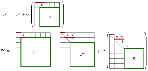
Figure 6: Decomposition of DOAG labelled transition matrices based or their content near the top of the diagonal. The symbols $\mathcal{D}$ and ${\mathcal{D}}^{\star}$ respectively represent the set of all possible DOAG labelled transition matrices the set of all of those matrices such that $a_{1,2}>0$. The stars $(\star)$ represent strictly positive values.

We compute the contributions to $D_{n}$ coming from each of these four terms described above. Let us denote by $D_{n}^{\star}$ the number of DOAG of size $n$ with exactly one source, or equivalently the number of DOAG labelled transition matrices containing a non-zero value at coordinates $(1,2)$. The first line of Figure 6 illustrates the first point of the decomposition, which yields

$$D_{n}=D_{n}^{\star}+O(v_{n-2}D_{n-1}).$$ (8)

Note that the big oh comes from the fact that not all pairs made of a size-$(n-2)$ variation and a size-$(n-1)$ labelled transition matrix can be obtained this way, as discussed in the first case above.

Then we decompose the matrices from ${\mathcal{D}}^{\star}$ depending of their values on the diagonal (cases 2 to 4). The second line of Figure 6 illustrates this decomposition. This translates into the following identity

$$D_{n}^{\star}=(v_{n-1}-v_{n-2})D_{n-1}^{\star}+\frac{v_{n-1}-2v_{n-2}+v_{n-3}}{2}v_{n-3}D_{n-2}^{\star}+O\!\left(v_{n-1}v_{n-3}v_{n-4}D_{n-3}\right).$$ (9)

Let us introduce the polynomial term $P_{n}^{\star}$ of $D_{n}^{\star}$ defined by $P_{n}^{\star}=D_{n}^{\star}/e^{n-1}\text{\normalshape¡}{n-1}!$. By normalising equation (8) and using equation (7) we have

$$P_{n}^{\star}=P_{n}+O\!\left(\frac{v_{n-2}}{e(n-1)!}P_{n-1}\right)=P_{n}+O\!\left(\frac{P_{n-1}}{n}\right)=P_{n}+o\!\left(P_{n}\right).$$

In other words, we have that $P_{n}$ and $P_{n}^{\star}$ are equivalent. Then, by normalising equation (9) by $e^{n-1}\text{\normalshape¡}{n-1}!$, we obtain the following asymptotic expansion

$$P_{n}^{\star}=\left(1-\frac{1}{n}+O\!\left(\frac{1}{n^{2}}\right)\right)P_{n-1}^{\star}+\frac{1}{2n}\left(1+O\!\left(\frac{1}{n}\right)\right)P_{n-2}^{\star}+O\!\left(\frac{P_{n-3}}{n^{2}}\right)\cdot$$ (10)

Since $P_{n}^{\star}\sim P_{n}$ and by equation (7), we have that $O\!\left(n^{-3}\right)=o\!\left(P_{n}^{\star}n^{-2}\right)$ and that the first term of equation (10) dominates all the others. As a consequence we get a refinement on our knowledge on $P_{n}^{\star}$ (and thus $P_{n}$), that is:

$$P_{n}^{\star}\sim P_{n-1}^{\star}.$$

By re-using this new information in equation (10), we get another term of the expansion of $P_{n}^{\star}$:

$$P_{n}^{\star}=P_{n-1}^{\star}\left(1-\frac{1}{2n}+O\!\left(\frac{1}{n^{2}}\right)\right).$$

We conclude on the asymptotic behaviour of $P_{n}^{\star}$ using the following classical argument. The series of general term $\ln\left(\!\frac{P_{n}^{\star}}{P_{n-1}^{\star}}\!\right)+\frac{1}{2n}=O\!\left(n^{-2}\right)$ (defined for $n\geq 2$) is convergent and, if $\lambda$ denotes its sum, we have that

$$\lambda-\sum_{j=2}^{n}\left(\ln\left(\!\frac{P_{j}^{\star}}{P_{j-1}^{\star}}\!\right)+\frac{1}{2j}\right)=O(n^{-1}).$$

Furthermore, since $P_{1}^{\star}=1$, we also have that

$$\sum_{j=2}^{n}\left(\ln\left(\!\frac{P_{j}^{\star}}{P_{j-1}^{\star}}\!\right)+\frac{1}{2j}\right)=\ln P_{n}^{\star}+\frac{1}{2}\left(\ln(n)+\gamma+O\!\left(n^{-1}\right)\right)$$

where $\gamma$ denotes the Euler–Mascheroni constant. As a consequence, we have that

$$\ln P_{n}^{\star}+\frac{\ln(n)}{2}=\lambda+\gamma+O\!\left(n^{-1}\right)$$

and thus

$$P_{n}^{\star}=\frac{e^{\lambda+\gamma}}{\sqrt{n}}\left(1+O\!\left(n^{-1}\right)\right).$$

By equation (8), we also get that $P_{n}=P_{n}^{\star}\left(1+O\!\left(n^{-1}\right)\right)$, which allows us to state the following theorem.

Theorem 4.

There exists a constant $C>0$ such that the number $D_{n}$ of DOAGs with $n$ vertices and the number $D_{n}^{\star}$ of such DOAGs having only one source satisfy

$$D_{n}=(1+O\!\left(n^{-1}\right))D_{n}^{\star}=\frac{C}{\sqrt{n}}\ e^{n-1}\ \text{\normalshape¡}{n-1}!\left(1+O\!\left(n^{-1}\right)\right).$$

The super factorial provides a concise way to express this equivalent and also reflects the relation between DOAGs and variation matrices. An equivalent without factorial can also be expressed using the formula from [Bar00] recalled in equation (3) above. For some constant $c$, we have

$$D_{n}\sim c\cdot n^{-7/12}\cdot{\big{(}e\sqrt{2\pi}\big{)}}^{n}\cdot e^{-\frac{3}{4}n^{2}}\cdot n^{n^{2}/2}.$$

5.3 Approximation of the constant

Let $D_{n,k}$ denote the number of DOAGs with $n$ vertices (including $k$ sources and one sink) and any number of edges. Using the same decomposition as in Section 2 and applying the same combinatorial arguments we get

$$D_{n,k}=\sum_{i+s\leq n-k}D_{n-1,k-1+s}\binom{s+i}{s}\binom{n-k-s}{i}i!=\sum_{s\geq 0}D_{n-1,k-1+s}\cdot\gamma(n-k-s,s)$$ (11)

where

$$\gamma(a,b)=\sum_{i=0}^{a}\binom{b+i}{b}\binom{a}{i}i!.$$ (12)

The above sum gives an explicit way to compute $\gamma$, but there is a computationally more efficient way to do so using recursion and memoisation:

$$\gamma(a,b) =0 a<0 b<0$$ when  or  (13)

$$\gamma(0,b) =1 b\geq 0$$ when 

$$\gamma(a,b) =\gamma(a,b-1)+a\cdot\gamma(a-1,b)+\boldsymbol{1}_{\{b=0\}}$$ otherwise.

Using this recurrence formula with memoisation, the numbers $D_{n,k}$ for all $n,k\leq N$ can be computed in $O(N^{3})$ arithmetic operations on big integers. Note that the $D_{n}^{\star}$ sequence defined above corresponds to $D_{n,1}$. Using the numbers computed by this algorithm, we plotted the first $250$ values of the sequences $D_{n}$ and $D_{n}^{\star}$ normalised by $n^{-1/2}e^{n-1}\text{\normalshape¡}{n-1}!$ which shows the convergence to the constant $C$ from Theorem 4. We also note that the convergence looks faster for the sequence $D_{n}^{\star}$. This suggests that the constant can be approximated by $C\approx 0.4967$. Figure 7 shows this plot as well as a zoomed-in version near $\frac{1}{2}$ for $n\geq 200$.

Figure 7: The first values of the sequences $\displaystyle{\frac{D_{n}\sqrt{n}}{\text{\normalshape¡}{n-1}!e^{n-1}}}$ in blue and $\displaystyle{\frac{D_{n}^{\star}\sqrt{n}}{\text{\normalshape¡}{n-1}!e^{n-1}}}$ in red.

5.4 Asymptotic behaviour of some parameters

5.4.1 Number of sources

It follows from the previous section that the probability that a uniform DOAG of size $n$ has more than one source tends to zero as $n\to\infty$. We can refine this result and compute the probability of having a constant number $k$ of sources.

We have that the number of sources of a DOAG is also the number of empty columns in its labelled transition matrix, and that these columns are necessarily in first positions. Moreover, Theorem 4 gives us the intuition that most of those transition matrices contain positive numbers near the top-left corner of the matrix. We thus split the set of matrices ${(a_{i,j})}_{1\leq i,j\leq n}$ encoding DOAGs with $k$ sources in two categories.

Case $\boldsymbol{a_{k,k+1}>0}$.

Intuitively, the most common scenario is that there is a positive entry in $a_{k,k+1}$. In this case the sub-matrix ${(a_{i,j})}_{k\leq i,j\leq n}$ can be re-interpreted as a DOAG with only one source. Indeed, the condition $a_{k,k+1}$ means that upon removing the $(k-1)$ first sources of the DOAG, the decomposition algorithm does not produce any new source, leaving us with a single-source DOAG. We can characterise those matrices: they are made of $(k-1)$ variations of size $(n-k)$ in the first rows, and a size-$(n-k+1)$ labelled transition matrix corresponding to a single source DOAG below them. Any combination of $(k-1)$ such variations and such matrices can be obtained.

Case $\boldsymbol{a_{k,k+1}=0}$.

On the other hand we have the matrices such that $a_{k,k+1}=0$. In this case, the $(k-1)$ first rows of the matrix are still variations of size $(n-k)$. The lower part ${(a_{i,j})}_{k\leq i,j\leq n}$ can be seen as a DOAG with at least two sources because its first two columns are empty. Note that here, depending of the $(k-1)$ top variations, we may have restriction on which DOAGs may appear in the lower part. For instance, if $k=2$ and the first row is $(0,0,1,0,0,\ldots,0)$, then the DOAG of size $(n-1)$ without any edge cannot appear in the lower part.

This dichotomy is pictured in Figure 8.

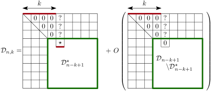
Figure 8: Decomposition of the matrices corresponding to DOAGs with $k$ sources

From the above case analysis, we have the following bounds:

$$v_{n-k}^{k-1}D_{n-k+1}^{\star}\leq D_{n,k}\leq v_{n-k}^{k-1}D_{n-k+1}+O\!\left(v_{n-k}^{k-1}(D_{n-k+1}-D_{n-k+1}^{\star})\right).$$

Thus, by virtue of Theorem 4, we have the following estimates when $(n-k)\to\infty$

$$D_{n,k}=v_{n-k}^{k-1}D_{n-k+1}^{\star}\left(1+O\!\left(\frac{1}{n-k}\right)\right),$$ (14)

which allow us to state the following result.

Theorem 5 (Number of sources of uniform DOAGs).

When $n\to\infty$ and $(n-k)\to\infty$, we have that

$$D_{n,k}-v_{n-k}^{k-1}D_{n-k+1}=o(D_{n,k})$$

where the little oh is uniform: it is arbitrarily smaller than $D_{n,k}$ when $(n-k)\to\infty$. In particular for $k$ constant, we have

$$\frac{D_{n,k}}{D_{n}}\sim n^{-\binom{k}{2}}.$$

Proof.

The first statement has already been established in equation (14) and the second one is straightforward to obtain using the equivalent $v_{n}\sim en{!}$ for the number of variations. ∎

5.4.2 Number of edges

Another quantity of interests of uniform DOAGs (and graphs in general) is their number of edges. Whereas uniform labelled DAGs have $\frac{n^{2}}{4}$ edges in average, we show here that the number of edges of uniform DOAGs is close to $\frac{n^{2}}{2}$. This has to be compared with their maximum possible number of edges which is $\binom{n}{2}=\frac{n(n-1)}{2}$. This makes uniform DOAGs quite dense objects. The intuition behind this fact is that variations have typically few zeros in them. Indeed, the expected number of zeros of a uniform variation is given by

$$\frac{1}{v_{n}}\sum_{p=0}^{n}pv_{n,p}=\frac{n!}{v_{n}}\sum_{p=0}^{n}\frac{p}{p!}=\frac{n!}{v_{n}}\sum_{p=1}^{n}\frac{1}{(p-1)!}\underset{n\to\infty}{\to}1$$

where $v_{n,p}$ is the number of variations of size $n$ having exactly $p$ zeros, which is equal to $n!/p{!}$ by Lemma 4. Moreover, the tail of their probability distribution is more than exponentially small:

$$\mathbb{P}_{n}[\text{nb zeros}\geq q]=\frac{n!}{v_{n}}\sum_{p=q}^{n}\frac{1}{p!}\underset{n,q\to\infty}{=}\frac{e^{-1}}{q!}\left(1+o\!\left(\frac{1}{n!}\right)\right)\left(1+O\!\left(\frac{1}{q}\right)\right),$$

where the first error term depends only on $n$ and the second depends on $q$ and is uniform in $n$. Now, recall that DOAG labelled transition matrices are a sub-class of variations matrices, and that the number of non-zero entries in these matrices corresponds to the number of edges of the graph. This discussion should make the following result intuitive.

Theorem 6 (Number of edges of uniform DOAGs).

The number of edges of a uniform DOAG of size $n$ is, in expectation,

$$\binom{n}{2}-O(n).$$

Proof.

In terms of labelled transition matrices, the theorem translates into: there is at most a linear number of zeros strictly above the diagonal in the matrix. This is what we prove here.

For all integer $p\geq 0$, by inclusion, we have that the number of DOAG labelled transition matrices with exactly $p$ zeros strictly above the diagonal is upper-bounded by the number $\operatorname{\mathrm{VM}}_{n,p}$ of variation matrices with the same property. Moreover, given a vector $(p_{1},p_{2},\ldots,p_{n-1})$ of non-negative integers such that for all $i$, $p_{i}\leq i$, the number of such variation matrices with exactly $p_{n-i}$ zeros in the $i$-th line is

$$\prod_{i=1}^{n-1}v_{i,p_{i}}=\prod_{i=1}^{n-1}\frac{i!}{p_{i}!}=\text{\normalshape¡}{n-1}!\prod_{i=1}^{n-1}\frac{1}{p_{i}!}.$$

By summation over all such vectors such that $\sum_{i=1}^{n-1}p_{i}=p$, we get an expression for $\operatorname{\mathrm{VM}}_{n,p}$:

$$\operatorname{\mathrm{VM}}_{n,p}=\text{\normalshape¡}{n-1}!\sum_{\begin{subarray}{c}p_{1}+p_{2}+\cdots+p_{n-1}=p\\ \text{for all~{}$i$},0\leq p_{i}\leq i\end{subarray}}\prod_{i=1}^{n-1}\frac{1}{p_{i}!}\leq\text{\normalshape¡}{n-1}!\sum_{\begin{subarray}{c}p_{1}+p_{2}+\cdots+p_{n-1}=p\\ \text{for all~{}$i$},0\leq p_{i}\end{subarray}}\prod_{i=1}^{n-1}\frac{1}{p_{i}!}\cdot$$

In the first sum we have the constraint $p_{i}\leq i$ because a variation has at most $i$ zeros. The inequality comes from the fact that we added more terms in the sum by dropping this constraints. This allows us to interpret the sum as a Cauchy product and can express it as the $p$-th coefficient of the power series $e^{x}\cdot e^{x}\cdot\cdots\cdot e^{x}=e^{(n-1)x}$. It follows that

$$\operatorname{\mathrm{VM}}_{n,p}\leq\text{\normalshape¡}{n-1}!\frac{{(n-1)}^{p}}{p!}\cdot$$

As a consequence, we have the following bound for the probability that a uniform DOAG of size $n$ has at most $\binom{n}{2}-q$ zeros:

$$\mathbb{P}_{n}[\text{a uniform DOAG has at most~{}$\binom{n}{2}-q$ zeros}]\leq\frac{\text{\normalshape¡}{n-1}!}{D_{n}}\sum_{p\geq q}\frac{{(n-1)}^{p}}{p!}\cdot$$ (15)

The sum in the last equation is the remainder in the Taylor expansion of order $(q-1)$ of the function $e^{x}$ near zero, evaluated at the point $(n-1)$. By using the integral form of this remainder, we have that

$$\sum_{p\geq q}\frac{{(n-1)}^{p}}{p!}=\int_{0}^{n-1}e^{t}\frac{{(n-1-t)}^{q-1}}{(q-1)!}dt\leq e^{n-1}\int_{0}^{n-1}\frac{{(n-1-t)}^{q-1}}{(q-1)!}dt=e^{n-1}\frac{{(n-1)}^{q}}{q!}\cdot$$

Furthermore, by setting $q=\lambda(n-1)$ for some constant $\lambda>0$, and by using Stirling’s formula, we get that

$$\frac{{(n-1)}^{q}}{q!}\sim{\left(\frac{e(n-1)}{q}\right)}^{q}\frac{1}{\sqrt{2\pi q}}\sim{\left(\frac{e^{\lambda}}{\lambda^{\lambda}}\right)}^{n-1}\frac{1}{\sqrt{2\pi\lambda n}}\cdot$$

Finally, by using this estimate inside equation (15), and by using of Theorem 4 for estimating $D_{n}$, we get that there exists a constant $c>0$ such that

$$\mathbb{P}_{n}[\text{a uniform DOAG has at most~{}$\binom{n}{2}-\lambda(n-1)$ zeros}]\leq\frac{\text{\normalshape¡}{n-1}!e^{n-1}}{D_{n}}\sum_{p\geq q}\frac{{(n-1)}^{q}}{q!}\leq\frac{c}{\sqrt{\lambda}}{\left(\frac{e^{\lambda}}{\lambda^{\lambda}}\right)}^{\mathclap{\,\,n-1}}\cdot$$

The latter expression is exponentially small as soon as $\lambda>e$ and dominates the tail of the probability distribution of the number of zeros strictly above the diagonal in DOAG labelled transition matrices, which allows to conclude. ∎

6 Uniform sampling of DOAGs by vertices only

The knowledge from the previous section on the asymptotic number of DOAGs with $n$ vertices can be interpreted combinatorially to devise an efficient uniform random sampler of DOAGs based on rejection. Since the set of labelled transition matrices of size $n$ is included in the set of variation matrices of size $n$, a possible approach to sample uniform DOAGs is to sample uniform variation matrices until they satisfy the properties of Theorem 3, and thus encode a DOAG.

Since the number of variation matrices is close (up to a factor of the order of $\sqrt{n}$) to the number of DOAGs, the probability that a uniform variation matrix of size $n$ corresponds to the labelled transition matrix of DOAG is of the order of $n^{-\frac{1}{2}}$. As a consequence, the expected number of rejections done by the procedure outline above is of the order of $\sqrt{n}$ and its overall cost is $\sqrt{n}$ times the cost of generating one variation matrix. Moreover, we will see that variations (and thus variation matrices) are cheap to sample, which makes this procedure efficient.

This idea, which is a textbook application of the rejection principle, already yields a reasonably efficient sampler of DOAGs. In particular it is much faster than the sampler from the previous section based on the recursive method, because it does not have to carry arithmetic operations on big integers. In this section we show that this idea can be pushed further using “early rejection”. That is to say we check the conditions from Theorem 3 on the fly when generating the variation matrix, in order to be able to abort the generation as soon as possible if the matrix is to be rejected. We will describe how to generate as few elements of the matrix as possible to decide whether to reject it or not, so as to mitigate the cost of these rejections.

First, we design an asymptotically optimal uniform sampler of variations in Section 6.1, and then we show in Section 6.2 how to leverage this into an asymptotically optimal sampler of DOAGs.

6.1 Generating variation

The first key step towards generating DOAGs, is to describe an efficient uniform random sampler of variations. We observe that the law of the number of zeros of a uniform variation of size $n$ obeys a Poisson law of parameter $1$ conditioned to be at most $n$. Indeed,

$$\mathbb{P}[\text{a uniform variation of size~{}$n$ has~{}$p$ zeros}]=\frac{v_{n,p}}{v_{n}}\propto\frac{\boldsymbol{1}_{\{0\leq p\leq n\}}}{p!}$$

by Lemma 4. A possible way to generate a uniform variation is thus to draw a Poisson variable $p$ of parameter $1$ conditioned to be at most $n$, and then shuffling a size $p$ array of zeros with a uniform permutation using the Fisher-Yates algorithm [FY48]. This is described in Algorithm 3.

Algorithm 3 Uniform random sampler of variations based on the rejection principle.

1:An integer $n>0$

2:A uniform random variation of size $n$

3:function UnifVariation($n$)

4:     $p$ $\leftarrow$ BoundedPoisson($1,n$)

5:     $A$ $\leftarrow$ $[0,0,\ldots,0,1,2,\ldots,n-p]$$\triangleright$ array of length $n$, starting with $p$ zeros

6:     for $i=0$ to $n-2$ do

7:         $r$ $\leftarrow$ Unif($\llbracket i;n-1\rrbracket$)

8:         $A[r]\leftrightarrow A[i]$ $\triangleright$ Swap entries of indices $r$ and $i$      

9:     return $A$

Regarding the generation of the bounded Poisson variable (performed at line 4), an efficient approach is to generate regular (unbounded) Poisson variables until a value less than $n$ is found. Since a Poisson variable of parameter $1$ has a high probability to be small, this succeeds in a small bounded number of tries on average. The algorithm described by Knuth in [Knu97, page 137] is suitable for our use-case since our Poisson parameter ($1$ here) is small. Furthermore it can be adapted to stop early when values strictly larger than $n$ are found. This is described in Algorithm 4.

Algorithm 4 Adapted Knuth’s algorithm for bounded Poisson simulation

1:A Poisson parameter $\lambda>0$ and an integer $n\geq 0$

2:A Poisson variable of parameter $\lambda$ conditioned to be at most $n$

3:function BoundedPoisson($\lambda,n$)

4:     repeat

5:         $k$ $\leftarrow$ $0$

6:         $p$ $\leftarrow$ Unif($[0;1]$)

7:         while $(k\leq n)\wedge(p>e^{-\lambda})$ do

8:              $k$ $\leftarrow$ $k+1$

9:              $p$ $\leftarrow$ $p\cdot\text{{Unif}($[0;1]$)}$          

10:     until $k\leq n$

11:     return $k$

NB. The $\textsc{Unif}([0;1])$ function generates a uniform real number in the $[0;1]$ interval.

Note that this algorithm relies on real numbers arithmetic. In practice, approximating these numbers by IEEE 754 floating points numbers [Soc08] should introduce an acceptably small error. Indeed, since we only compute products (no sums or subtractions), which generally have few terms, the probability that they introduce an error should not be too far from $2^{-53}$ on a 64-bits architecture. Of course this is only a heuristic argument. A rigorous implementation must keep track of these errors. One possible way would be to use fixed points arithmetic for storing $p$ and to lazily generate the base 2 expansions of the uniform variables at play until we have enough bits to decide how $p$ and $e^{-\lambda}$ compare at line 7. Another way would be to use Ball arithmetic [Hoe10, Joh17] and to increase precision every time the comparison requires more bits. The proofs of correctness and complexity below obviously assume such an implementation.

Lemma 7 (Correctness of Algorithm 3).

Given an input $n>0$, Algorithm 3 produces a uniform random variation of size $n$.

Proof.

The correctness of Algorithm 4 follows from the arguments given in [Knu97, page 137], which we do not recall here. Regarding Algorithm 3, the for loop at line 6 implements the Fisher-Yates [FY48] algorithm, which performs a uniform permutation of the contents of the array independently of its contents. In our use-case, this implies that:

• the number of zeros is left unchanged;

• given an initial array with $p$ zeros as shown at line 5, the probability to get a particular variation with $p$ zeros is given by the probability that a uniform permutations maps its first $p$ values to a prescribed subset of size $p$, that is $\frac{p!}{n!}$.

This tells us that, the probability that Algorithm 3 yields a particular variation with $p$ zeros is

$$\mathbb{P}[\textsc{BoundedPoisson}(1,n)=p]\cdot\frac{p!}{n!}=\frac{1}{p!\sum_{k=0}^{n}\frac{1}{k!}}\cdot\frac{p!}{n!}=\frac{1}{v_{n}}.\qed$$

The “amount of randomness” that is necessary to simulate a probability distribution is given by its entropy. This gives us a lower bound on the complexity (in terms of random bit consumption) of random generation algorithms. For uniform random generation, this takes a simple form since the entropy of a uniform variable that can take $M$ distinct values is $\log_{2}(M)$. This tells us that we need at least $\log_{2}(v_{n})$ random bits to generate a uniform variation of size $n$. When $n$ is large, we have $\log_{2}(v_{n})=n\log_{2}(n)-\frac{n}{\ln(2)}+O(\log_{2}(n))$. The uniform variation sampler we give in Algorithm 3 is asymptotically optimal in terms of random bit consumption: in expectation, the number of random bits that it uses is equivalent to $\log_{2}(v_{n})$.

Lemma 8 (Complexity of Algorithm 3).

In expectation, Algorithm 3 consumes $n\log_{2}(n)+o(n\log_{2}(n))$ random bits and performs a linear number of arithmetic operations and memory accesses.

Proof.

The means of a Poisson variable of parameter $1$ being $1$, Algorithm 4 succeeds to find a value smaller or equal to $n$ in a constant number of tries in average, and each try requires a constant number of uniform variables in average. Furthermore, in order to perform the comparison $p>e^{-1}$ at line 7 in the algorithm, we need to evaluate these uniform random variables. This can be done lazily, and again, it is sufficient to know a constant number of bits of these variables in average to decide whether $p>e^{-1}$.

Regarding the shuffling happening at line 6 in Algorithm 3, it needs to draw $(n-1)$ uniform integers, respectively smaller or equal to $1$, $2$, $3$, …, $n-1$. At the first order, this incurs a total cost in terms of random bits, of

$$\sum_{k=2}^{n}\log_{2}(k)\sim n\log_{2}(n).$$

In total, the cost of Algorithm 3 is thus dominated by the shuffling, which allows to conclude on its random bits complexity.

Regarding the number of arithmetic operations and memory accesses, generating Poisson variables performs in constant time using similar arguments. The shuffling part of the algorithm is clearly linear. ∎

Note that we count integer operations in the above Lemma, thus abstracting away the cost of these operations. At the bit level an extra $\log_{2}(n)$ term would appear to take into account the size of these integers. This type of considerations is especially important when working with big integers as it was the case in Section 2. However here, arithmetic operations on integers, rather than bits, seems to be the right level of granularity as a real-life implementation is unlikely to overflow a machine integer.

6.2 A fast rejection procedure

Equipped with the variation sampler described above, we can now generate variation matrices in an asymptotically optimal way, by filling them with variations of sizes $(n-1),(n-2),\ldots,3,2,1$. By checking afterwards whether the matrix corresponds to a valid DOAGs, and trying again if not, we get a uniform sampler of DOAGs that is only sub-optimal by a factor of the order of $\sqrt{n}$. This is presented in Algorithm 5. This algorithm is already more efficient than a sampler based on the recursive method, whilst naive.

Algorithm 5 A simple but sub-optimal uniform random sampler of DOAGs

An integer $n>0$

A uniform DOAG with $n$ vertices as its labelled transition matrix

function UnifDOAGNaive($n$)

     $A={(a_{i,j})}_{1\leq i,j\leq n}$ $\leftarrow$ a zero-filled $n\times n$ matrix

     repeat

         for $i$ from $1$ to $n-1$ do

              ${(a_{i,j})}_{i<j\leq n}$ $\leftarrow$ UnifVariation($n-i$)          

     until $A$ encodes a DOAG

     return The DOAG corresponding to $A$

Checking the validity of a matrix at line 8 corresponds to checking the conditions given in Theorem 3 at page 3. We do not provide an algorithm for this here, as the goal of this section is to iterate upon Algorithm 5 to provided a faster algorithm and get rid of the $\sqrt{n}$ factor in its cost. We will see in the following that checking these conditions can be done in linear time.

As we can see in Theorem 3, the conditions that a variation matrix must satisfy to be a labelled transition matrix, concern the shape of boundary between the zero-filled region between the diagonal and the first positive values above the diagonal. Moreover, we have seen in Theorem 6 that uniform DOAGs tend to have close to $\binom{n}{2}$ edges and thus only a linear number of zeros above the diagonal of their labelled transition matrix. We can thus expect that the area that we have to examine to have access to this boundary should be small. This heuristic argument, hints at a more sparing algorithm that would start by filling the matrix near the diagonal and check its validity early, before generating the content of the whole matrix. This idea, of performing rejection as soon as possible in the generation process, is usually referred to as “anticipated rejection” and also appears in [Duc+04] and [BPS94] for instance.

To put this idea in practice, we need to implement lazy variation generation, to be able to make progress in the generation of each line independently, and to perform the checks of Theorem 3 while requiring as little information as necessary.

Ingredient one: lazy variations

Fortunately, Algorithm 3 can be easily adapted for this purpose thanks to the fact that the for loop that implements the shuffle progresses from left to right in the array. So a first ingredient of our optimised sampler is the following setup for lazy generation:

• for each row of the matrix (i.e. each variation to be sampled), we draw a Poisson variable $p_{i}$ of parameter $1$ and bounded by $(n-i)$;

• drawing the number at position $(i,j)$, once we have drawn all the numbers of lower coordinate in the same row, can be done by selecting uniformly at random a cell with higher or equal coordinate on the same row and swapping their contents.

This is illustrated in Figure 9.

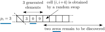
Figure 9: Ingredient one of the fast rejection-based algorithm: variations can be lazily generated. In the example, the three first elements of the variation at row $i$ are known. When we need to generate its fourth element, we perform a swap of $a_{i,i+4}$ with a uniform cell of index $j\geq i+4$.

Ingredient two: only one initialisation

A straightforward adaptation of Algorithm 3 unfortunately requires to re-initialise the rows after having drawn the Poisson variable (see line 5 of Algorithm 3) at each iteration of the rejection algorithm. This is costly since about $n^{2}/2$ numbers have to be reset. It is actually possible to avoid this by initialising all the rows only once and without any zeros. Only at the end of the algorithm, once a full matrix have been generated, one can re-interpret the $p_{i}$ largest numbers of row $i$, for all $i$, to be zeros. This is pictured in Figure 10.

Figure 10: Ingredient two of the fast rejection-based algorithm: the zeros of the matrix need not be explicitly written. Instead, we interpret the numbers strictly larger than $(n-i-p_{i})$ as zeros. In this example $(n-i)=10$ and $p_{i}=3$ so the numbers $8$, $9$, and $10$ are seen as zeros.

Ingredient three: column by column checking

The last detail that we need to explain is how to check the conditions of Theorem 3. As a reminder

• for each $2\leq j\leq n$ we need to compute the number $b_{j}=\max\,\{i\ |\ a_{i,j}>0\}$ (or $0$ is this set is empty);

• we must check whether this sequence is weakly increasing;

• and whenever $b_{j+1}=b_{j}$, we must check that $a_{b_{j},j}<a_{b_{j},j+1}$.

A way of implementing this is to start filling each column of the matrix from bottom to top, starting from the column $j=1$ and ending at column $j=n$. For each column, we stop as soon as either a non-zero number is found or the constraints from Theorem 3 are violated. In order to check these constraints, while filling column $j$ from bottom $(i=j-1)$ to top, we halt as soon as either the cell on the left of the current cell, or the current cell is non-zero. The case when the left cell is non-zero corresponds to when $i=b_{j-1}$ and the conditions of Theorem 3 can be checked. Recall that, per the previous point, the zero test in row $i$ is actually $x\mapsto x>n-i-p_{i}$. We shall prove that this process uncovers only a linear number of cells of the matrix, thus allowing to reject invalid matrices in linear expected time. This idea is pictured in Figure 11.

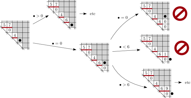
Figure 11: Ingredient three of the fast rejection-based algorithm: the exploration process of the cell of the matrix follows a strict discipline. We proceed column by column, from bottom to top, and we change columns as soon as we see a non-zero cell on our left. In the pictures, the bullet $\bullet$ represent the current cell, the grey area represents the cells that have not yet been drawn and the thick red lines underline the lowest non-zero cell of each column, as before. Depending on the value that is drawn in the current cell, we either move up or to the next column. Whenever a non-zero cell is on our left, we can decide whether to reject or to keep generating.

The algorithm

Putting all of this together yields Algorithm 6 to generate a uniform DOAG labelled transition matrix using anticipated rejection. The algorithm is split to two parts. First, the repeat-until loop between lines 7 and 22 implements the anticipated rejection phase. At each iteration of this loop, we “forget” what has been done in the previous iterations, so that $A$ is considered to be an arbitrary matrix satisfying the following two conditions

$$i\geq j\implies a_{i,j}=0$$ (16)

$$\forall~{}1\leq i<n,\quad\{a_{i,j}\,|\,i<j\leq n\}=\llbracket 1;n-i\rrbracket.$$ (17)

The contents of the ${(p)}_{1\leq i<n}$ vector is also forgotten and each value is to be drawn again before any access. The while loop at line 10 implements the traversal of the matrix described above: at each step, the value of the $a_{i,j}$ is drawn and the conditions of Theorem 3 are checked before proceeding to the next step. The array ${(s_{i})}_{1\leq i\leq n}$ stores the state of each lazy variation generator: $s_{i}$ contains the value of the largest $j$ such that $a_{i,j}$ has been drawn. The second part of the algorithm, starting from line 23, completes the generation of the matrix once its near-diagonal part is known and we know no rejection is possible any more. This includes replacing some values of the matrix by $0$ per ingredient two above.

Algorithm 6 An optimised uniform random sampler of DOAGs based on anticipated rejection

1:An integer $n>0$

2:A uniform DOAG with $n$ vertices, encoded as its labelled transition matrix.

3:function UnifDOAGFast($n$)

4:     $A={(a_{i,j})}_{1\leq i,j\leq n}$ $\leftarrow$ the strictly upper triangular matrix ${(\boldsymbol{1}_{\{j>i\}}\cdot(j-i))}_{1\leq i,j\leq n}$

5:     ${(p_{i})}_{1\leq i<n}$ $\leftarrow$ uninitialised array

6:     ${(s_{i})}_{1\leq i<n}$ $\leftarrow$ uninitialised array

7:     repeat$\triangleright$ Anticipated rejection phase

8:         $(i,j)$ $\leftarrow$ $(1,2)$$\triangleright$ position of the current cell

9:         $p_{1}$ $\leftarrow$ BoundedPoisson($n-1$)

10:         while $j\leq n$ do

11:              $r$ $\leftarrow$ Unif($\llbracket j;n\rrbracket$)

12:              $a_{i,r}\leftrightarrow a_{i,j}$

13:              $s_{i}$ $\leftarrow$ $j$

14:              if $(a_{i,j-1}\leq n-i-p_{i})\wedge(a_{i,j}\not\in\llbracket a_{i,j-1}+1;n-i-p_{i}\rrbracket)$ then

15:                  break$\triangleright$ Rejection

16:              else if $a_{i,j}\leq n-i-p_{i}$ then

17:                  $j$ $\leftarrow$ $j+1$

18:                  $i$ $\leftarrow$ $j-1$

19:                  $p_{i}$ $\leftarrow$ BoundedPoisson($1,n-i$)

20:              else

21:                  $i$ $\leftarrow$ $i-1$                         

22:     until $j>n$

23:     for $i=1$ to $n-2$ do$\triangleright$ Completion of the matrix

24:         for $j=i+1$ to $s_{i}$ do

25:              if $a_{i,j}>n-i-p_{i}$ then $a_{i,j}\leftarrow 0$                        

26:         for $j=s_{i}+1$ to $n$ do

27:              $r$ $\leftarrow$ Unif($\llbracket j;n\rrbracket$)

28:              $a_{i,r}\leftrightarrow a_{i,j}$

29:              if $a_{i,j}>n-i-p_{i}$ then $a_{i,j}\leftarrow 0$                              

30:     return $A$

Lemma 9 (Correction of Algorithm 6).

Algorithm 6 terminates with probability $1$ and returns a uniform random DOAG labelled transition matrix.

This result is a consequence of Algorithm 5 and Algorithm 6 implementing the exact same operations, only in a different order and with an earlier rejection in the latter algorithm. The key characteristic of this new algorithm is that is only needs to perform a linear number of swaps in average to decide whether the reject the matrix or not. As a consequence it is asymptotically optimal in terms of random bits consumption and it only performs about $n^{2}/2$ swaps to fill the $n\times n$ upper triangular matrix.

Theorem 7 (Complexity of Algorithm 6).

In average, Algorithm 6 consumes $\frac{n^{2}}{2}\log_{2}(n)+O(n^{3/2}\log_{2}(n))$ random bits and performs $\frac{n^{2}}{2}+O(n^{3/2})$ swaps in the matrix.

Proof.

In the rejection phase, in each column, we draw a certain number of zeros and at most one non-zero value before deciding whether to reject the matrix or to proceed to the next column. As a consequence, when lazily generating a variation matrix, we see at most $(n-1)$ non-zero values and a certain number of zeros that we can trivially upper-bound by the total number of zeros (strictly above the diagonal) in the matrix.

The number of variations of size $n$ with exactly $p$ zeros (with $0\leq p\leq n$) is given by $\frac{n!}{p!}$ by Lemma 4. As a consequence, the expected number of zeros of a variation is given by

$$\sum_{p=0}^{n}p\cdot\frac{n!}{p!}\cdot\frac{1}{v_{n}}=\left(e^{-1}+o\!\left(\frac{1}{n!}\right)\right)\sum_{p=0}^{n-1}\frac{1}{p!}=1+O\!\left(\frac{1}{n!}\right).$$

It follows that the expectation of the total number of zeros of variation matrix of size $n$ is $n+O(1)$. This proves the key fact that, in expectation, we only discover a linear number of cells of the matrix in the repeat-until loop. Since, in expectation, we only perform $O(\sqrt{n})$ iteration of this loop, it follows that we only perform $O(n^{3/2})$ swaps there. Moreover, one swap costs $O(\log_{2}(n))$ random bits, which thus accounts for a total of $n^{3/2}\log_{2}(n)$ random bits in this loop.

In order to complete the proof, it remains to show that the for loops at the end of Algorithm 6 contribute to the leading terms of the estimates given in the Theorem. The first inner for loop at line 24 replaces, among the already discovered values, the zeros encoded by numbers above the $n-i-p_{i}$ threshold by actual zeros. It is worth mentioning that this only accounts for linear number of iterations in total, spanned over several iteration of the outer loop (at line 23). The second inner for loop at line 26 completes the generation of the matrix. The total number of swaps that it performs (and thus the number of uniform variables it draws) is $\frac{n(n-1)}{2}$ minus the number of already discovered cells, that is $n^{2}/2+O(n)$. This allows to conclude the proof. ∎

Using equation (5.2), just bellow Theorem 4, we have that $\log_{2}(D_{n})\sim\frac{n^{2}}{2}\log_{2}(n)$. This shows that Algorithm 6 is asymptotically optimal in terms of random bit consumption. Moreover, filling a $n\times n$ matrix requires a quadratic number of memory writes and the actual number of memory access made by our algorithm is of this order too.

7 Extension to labelled DAGs

In this last section we demonstrate the applicability of our method by establishing a counting formula for the classical model of labelled DAGs, counted by vertices, edges, and sources. This corresponds to a sequence obtained by Gessel in [Ges96] using a generating functions approach. The recurrence relations we obtain here are different and in particular they involve no subtraction, which makes them amenable to effective random sampling. To our knowledge, this is the first such formula for labelled DAGs.

The difference between the formula presented here and the one given in our previous work [GPV21] is that here we take all DAGs into account, not only those with one sink. But we are also able to specialise the formula to some sub-classes, like we did for DOAG in Section 2.1.1.

7.1 Recursive decomposition

In a first attempt to decompose regular vertex-labelled DAGs, one might be tempted to devise a decomposition similar to DOAGs by removing the smallest source at each step. However, in this case this makes the recurrence difficult to express. Instead we count vertex-labelled DAGs with a distinguished source (this operation is called pointing), which makes the decomposition much simpler as we do not have to maintain an ordering.

Let $A_{n,m,k}$ denote the number of labelled DAGs with $n$ vertices, $k$ sources, $m$ edges, and any number of sinks. Just like DOAGs, these objects are thus not necessarily connected. The number of such DAGs with a distinguished (or pointed) source is given by $k\cdot A_{n,m,k}$ since any of the $k$ sources may be distinguished. Let $D$ denote one such DAG and let $v$ denote its distinguished source. Removing the distinguished source in $D$ and decrementing the labels of the vertices of higher label than $v$ by one yields a regular vertex-labelled DAG $D^{\prime}$ with $n-1$ vertices. Moreover, the three pieces of information that are necessary to reconstruct the source are the following:

1. the label $\ell$ of the source $v$ which has been removed;

2. the set $S$ of sources of $D^{\prime}$ which have been uncovered by removing $v$;

3. the set $I$ of internal (non-sources) vertices of $D^{\prime}$ that were pointed at by $v$.

The reconstruction is then straightforward:

• increment all the labels that are greater or equal to $\ell$ by one;

• create a new vertex labelled $\ell$ and “mark” it: this is the distinguished source;

• add edges from $\ell$ to all the vertices from $S$ and $I$.

This decomposition differs from that of DOAGs in that we have not ordering to maintain on the set of vertices of the DAG, hence any subset $S$ of the set of sources of $D^{\prime}$ is licit here. The triplet $(\ell,S,I)$ is thus not constrained which leads to a simple counting formula. This leads to the following recursive formula where $p$ denotes the out-degree of $v$ (and thus the cardinality of $S\cup I$ using the notations from above).

$$A_{1,m,k} =\boldsymbol{1}_{\{m=0~{}\wedge~{}k=1\}}$$ (18)

$$A_{n,m,k} =0 \text{when}~{}k\leq 0~{}\text{or}~{}k>n$$

$$A_{n,m,k} =\frac{n}{k}\sum_{p=0}^{n-k}\sum_{i=0}^{p}A_{n-1,m-p,k-1+p-i}\binom{n-k-p+i}{i}\binom{k-1+p-i}{p-i}$$ otherwise.

Here, the first binomial coefficient $\binom{n-k-p+i}{i}$ counts the number of possibilities for the set $I$ of edges to internal vertices. The second binomial coefficients $\binom{k-1+p-i}{p-i}$ counts the number of possibilities for the other edges: that than point at sources of $D^{\prime}$.

Again, this formula counts all labelled DAGs, not only those with one sink. Computing the first terms of the sequence indeed yields the same numbers as the sequence A003024 in the OEIS and first enumerated in [Rob70, Sta73, Rob73]. Furthermore, as for DOAGs, we can capture some subclasses of labelled DAGs by putting restrictions on the out-degrees of the vertices. For instance, labelled DAGs with only one source and one sink can be counted by enforcing $p>0$ in the summation and computing $\sum_{m}A_{n,m,1}$. Computing the first terms of this sequence, we get back that values from A165950 in the OEIS related to the papers [Ges95, Ges96].

7.2 Random generation

A recursive random sampling algorithm similar to Algorithm 1 from Section 3 can be obtained from formula (18). The only difference in methodology from Algorithm 1 is that one has to deal with the marking of the sources here and thus the division by $k$ at the third line of (18). It can be handled as follows: at every recursive call, first generate a labelled DAG with a distinguished source (counted by $k\cdot A_{n,m,k}$) and then forget which source was distinguished. Since the recursive formula for $k\cdot A_{n,m,k}$ has no division, the uniform sampler of marked DAGs is obtained using the standard recursive method. Moreover, forgetting which source was marked does not introduce bias in the distribution since all sources have the same probability to be marked. A uniform random sampler of labelled DAGs with $n$ vertices, $k$ sources, and $m$ edges is described in Algorithm 7.

Algorithm 7 Uniform random sampler of vertex-labelled DAGs.

Three integers $(n,m,k)$ such that $A_{n,m,k}>0$

A uniform random vertex-labelled DAG with $n$ vertices (including $k$ sources and one sink), and $m$ edges

function sample($n,m,k$)

     if $n\leq 1$ then generate the (unique) labelled DAG with $1$ vertex

     else

         pick $(p,i)$ with probability $\displaystyle{A_{n-1,m-p,k-1+p-i}\binom{n-k-p+i}{i}\binom{k-1+p-i}{p-i}}/{A_{n,m,k}}$

         $D^{\prime}$ $\leftarrow$ sample($n-1,m-p,k-1+p-i$)

         $I$ $\leftarrow$ a uniform subset of size $i$ of the inner vertices of $D^{\prime}$

         $S$ $\leftarrow$ a uniform subset of size $(p-i)$ the sources of $D^{\prime}$

         $\ell$ $\leftarrow$ Unif($\llbracket 1;n\rrbracket$)

         relabel $D^{\prime}$ by adding one to all labels $\ell^{\prime}\geq\ell$

         return the DAG obtained by adding a new source to $D^{\prime}$ with label $\ell$ and $I\cup S$ as its out-edges      

Here again, since we can count some sub-classes of labelled DAGs by applying restrictions on the out-degree of the vertices in their recurrence formula (equation (18)), we can get an efficient uniform sampler for each of these sub-classes. This is achieved simply by using the new sequence in Algorithm 7, without any further changes. In particular, this gives access to a polynomial time algorithm for sampling labelled DAGs with small bounded degree, which is something that rejection-based approaches, or the Markov-Chain approach from [MDB01, KM15] would struggle at.

8 Conclusion and perspectives

In this paper, we have studied the new class of directed ordered acyclic graphs, which are directed acyclic graphs endowed with an ordering of the out-edges of each of their vertices. We have provided a recursive decomposition of DOAGs that is amenable to the effective random sampling of DOAGs with a prescribed number of vertices, edges and source using the recursive method from Nijenhuis and Wilf. Using a bijection with a class of integer matrices, we also have provided an equivalent for the number of DOAGs with $n$ vertices and designed an optimal uniform random sampler for them. We have also showed that our approach allows to approach classical labelled DAGs and have obtained a new recurrence formula for their enumeration. The important particularity is that this new formula is amenable to efficient random sampling when the number of edges is prescribed, which was not the case for previously known formulas.

Perspectives

An interesting question that is left open by our work is the case of the multi-graph variant of this model: what happens if multiple edges are allowed between two given vertices? This makes the analysis more challenging since their is now an infinite number of objects with $n$ vertices and we must thus take both vertices and edges into consideration directly. Estimating the number and behaviour of DOAGs as well as their multi-graph counterpart, when both parameters $n$ and $m$ grow remains an open question and will certainly yield very different results depending on how $n$ and $m$ grow in relation to each other.

Another interesting question is that of the connectivity. We do not provide a way to count connected DOAGs directly here. However we can already prove that in the uniform model from Section 5, their are connected with high probability since they have only one source with high probability. This implies that sampling a uniform connected DOAG with $n$ vertices is already possible, and efficient, by rejection. The question of the direct enumeration is thus mostly of mathematical interest.

Finally, it is also natural to wonder whether our successful approach at tackling the asymptotics of DOAG applies to labelled DAGs. Of course, this asymptotics is known [Ben+86]. But if a proof similar to ours is feasible, then it might be possible as well to devise an efficient, pre-computation-free, algorithm for sampling them. We are planning to investigate this question in the near future.

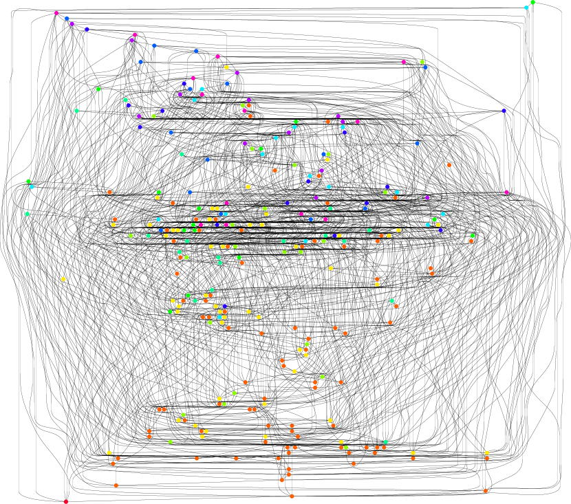
Figure 12: A random DOAG sampled uniformly at random among all DOAGs with $m=1000$ edges and with maximum out-degree bounded by $10$, that is such that all vertices have at most $10$ outgoing edges. This DOAG contains $272$ vertices. The colours of the vertices represent their out-degrees and have been picked according to the following colour map (lowest degree on the left and highest degree on the right).
. .

References

- [Bar00] Ernest William Barnes “The theory of the G-function” In The quarterly journal of pure and applied mathematics 31, 1900, pp. 264–314
- [Ben+86] Edward Anton Bender, Lawrence Bruce Richmond, Robert William Robinson and Nicholas Charles Wormald “The asymptotic number of acyclic digraphs” In Combinatorica 6.1 Springer, 1986, pp. 15–22
- [Bou+15] Mireille Bousquet-Mélou, Markus Lohrey, Sebastian Maneth and Eric Noeth “XML compression via directed acyclic graphs” In Theory of Computing Systems 57.4 Springer, 2015, pp. 1322–1371
- [BPS94] Elena Barcucci, Renzo Pinzani and Renzo Sprugnoli “The random generation of directed animals” In Theoretical Computer Science 127.2, 1994, pp. 333–350 DOI: 10.1016/0304-3975(94)90046-9
- [CEH19] Louis-Claude Canon, Mohamad El Sayah and Pierre-Cyrille Héam “A Comparison of Random Task Graph Generation Methods for Scheduling Problems” In European Conference on Parallel Processing 11725, LNCS, 2019, pp. 61–73 Springer DOI: 10.1007/978-3-030-29400-7“˙5
- [Cor+10] Daniel Cordeiro, Grégory Mounié, Swann Perarnau, Denis Trystram, Jean-Marc Vincent and Frédéric Wagner “Random graph generation for scheduling simulations” In 3rd International ICST Conference on Simulation Tools and Techniques (SIMUTools 2010), 2010, pp. 10 ICST
- [Duc+04] Philippe Duchon, Philippe Flajolet, Guy Louchard and Gilles Schaeffer “Boltzmann samplers for the random generation of combinatorial structures” In Combinatorics, Probability & Computing 13.4-5 Cambridge University Press, 2004, pp. 577–625
- [Ers58] Andrey Petrovych Ershov “On Programming of Arithmetic Operations” In Communications of the ACM 1.8 New York, NY, USA: Association for Computing Machinery, 1958, pp. 3–6
- [FY48] Ronald Aylmer Fisher and Frank Yates “Statistical tables for biological, agricultural and medical research” London: OliverBoyd, 1948
- [FZV94] Philippe Flajolet, Paul Zimmermann and Bernard Van Cutsem “A calculus for the random generation of labelled combinatorial structures” In Theoretical Computer Science 132.1-2 Elsevier, 1994, pp. 1–35
- [Gei+18] Kenneth Geisshirt, Emanuele Zattin, Aske Olsson and Rasmus Voss “Git Version Control Cookbook: Leverage Version Control to Transform Your Development Workflow and Boost Productivity, 2nd Edition” Packt Publishing, 2018
- [Ges95] Ira Martin Gessel “Enumerative applications of a decomposition for graphs and digraphs” In Discrete Mathematics 139.1, 1995, pp. 257–271 DOI: https://doi.org/10.1016/0012-365X(94)00135-6
- [Ges96] Ira Martin Gessel “Counting acyclic digraphs by sources and sinks” In Discrete Mathematics 160.1, 1996, pp. 253–258
- [Got74] Eiichi Goto “Monocopy and associative algorithms in an extended lisp”, 1974
- [GPV21] Antoine Genitrini, Martin Pépin and Alfredo Viola “Unlabelled ordered DAGs and labelled DAGs: constructive enumeration and uniform random sampling” In XI Latin and American Algorithms, Graphs and Optimization Symposium, 2021 Eslevier DOI: 10.1016/j.procs.2021.11.057
- [Hoe10] Joris Hoeven “Ball arithmetic” In Logical Approaches to Barriers in Computing and Complexity, 2010
- [Izq59] Sebastián Izquierdo “Pharus scientiarum” sumptibus Claudii Bourgeat & Mich. Lietard, 1659
- [Joh17] Fredrik Johansson “Arb: efficient arbitrary-precision midpoint-radius interval arithmetic” In IEEE Transactions on Computers 66, 2017, pp. 1281–1292 DOI: 10.1109/TC.2017.2690633
- [KM15] Jack Kuipers and Giusi Moffa “Uniform random generation of large acyclic digraphs” In Statistics and Computing 25.2, 2015, pp. 227–242
- [Knu97] Donald Ervin Knuth “The Art of Computer Programming, Volume 2, seminumerical algorithms” Addison-Wesley Longman Publishing Co., Inc., 1997
- [MDB01] Guy Melançon, Isabelle Dutour and Mireille Bousquet-Mélou “Random Generation of Directed Acyclic Graphs” In Electronic Notes in Discrete Mathematics 10, 2001, pp. 202–207 DOI: 10.1016/S1571-0653(04)00394-4
- [NW78] Albert Nijenhuis and Herbert Wilf “Combinatorial Algorithms: For Computers and Hard Calculators” USA: Academic Press, Inc., 1978
- [Rob70] Robert William Robinson “Enumeration of acyclic digraphs” In Proceedings of The Second Chapel Hill Conference on Combinatorial Mathematics and its Applications (Univ. North Carolina, Chapel Hill, NC, 1970), Univ. North Carolina, Chapel Hill, NC, 1970, pp. 391–399
- [Rob73] Robert William Robinson “Counting labeled acyclic digraphs” In New Directions in the Theory of Graphs Academic Press, 1973, pp. 239–273
- [Rob77] Robert William Robinson “Counting unlabeled acyclic digraphs” In Combinatorial Mathematics V, Lecture Notes in Mathematics Springer, 1977, pp. 28–43
- [Soc08] IEEE Computer Society “IEEE Standard for Floating-Point Arithmetic” In IEEE Std 754-2008, 2008, pp. 1–70 DOI: 10.1109/IEEESTD.2008.4610935
- [SP95] Neil James Alexander Sloane and Simon Plouffe “The encyclopedia of integer sequences” Academic Press, 1995
- [Sta11] Richard Peter Stanley “Enumerative Combinatorics” In Cambridge studies in advanced mathematics 1, 2011
- [Sta73] Richard Peter Stanley “Acyclic orientations of graphs” In Discrete Mathematics 5.2 Elsevier, 1973, pp. 171–178