BlobGAN-3D: A Spatially-Disentangled 3D-Aware
Generative Model for Indoor Scenes

Abstract

3D-aware image synthesis has attracted increasing interest as it models the 3D nature of our real world. However, performing realistic object-level editing of the generated images in the multi-object scenario still remains a challenge. Recently, a 2D GAN termed BlobGAN has demonstrated great multi-object editing capabilities on real-world indoor scene datasets. In this work, we propose BlobGAN-3D, which is a 3D-aware improvement of the original 2D BlobGAN. We enable explicit camera pose control while maintaining the disentanglement for individual objects in the scene by extending the 2D blobs into 3D blobs. We keep the object-level editing capabilities of BlobGAN and in addition allow flexible control over the 3D location of the objects in the scene. We test our method on real-world indoor datasets and show that our method can achieve comparable image quality compared to the 2D BlobGAN and other 3D-aware GAN baselines while being able to enable camera pose control and object-level editing in the challenging multi-object real-world scenarios.

1 Introduction

Generative Adversarial Networks (GANs) [17] have seen great success in generating highly-realistic images in various tasks [22, 70, 5, 11], and achieved state-of-the-art image quality [3, 28, 45, 46, 24]. Recently, a lot of exciting progress was made in 3D-aware image generation  [39, 71, 34, 47, 8, 9]. 3D-aware image generation is aiming at generating images that allow for explicit camera control. Different from approaches that require multiview images [39] or additional geometry supervision [71] as input, recent works focus on only utilizing single-view images to model the 3D nature of real-world objects [34, 47, 8, 9]. Nevertheless, current 3D-aware image generation mainly targets the synthesis of individual objects using a NeRF (Neural Radiance Field) [33, 67] representation. This yields good control for the properties of a single object, e.g. shape and texture, but it is not a suitable representation to learn the composition of a scene consisting of many individual objects.

Viewpoint

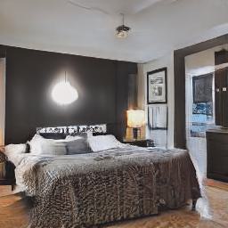
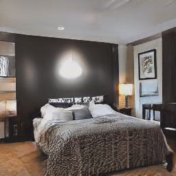
Moving

Restyling

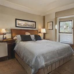
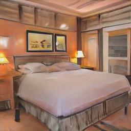
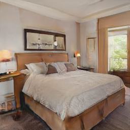
Figure 1: Images generated by BlobGAN-3D. Our method can control the viewpoint while enabling object-level editing like moving and restyling on a real-world indoor dataset.

For editing capabilities, multi-object scene editing is more challenging than single-object editing, as it requires disentanglement of individual objects. Ideally, a network should learn to distinguish individual objects without explicit supervision. Initial approaches towards that goal [15, 27, 13, 6, 2, 62, 57] have studied to manipulate the location or the pose of objects in 2D space in relatively simple synthetic datasets [21, 55, 6]. BlockGAN [35] adopts a 3D framework to a GAN backbone to model individual objects in a synthetic dataset. GIRAFFE [36] is a 3D-aware GAN that can manipulate single objects in real-world datasets and can scale to multi-object scenes thanks to its compositional modeling of scenes. However, for multi-object scenes, GIRAFFE can only manipulate synthetic datasets but fails to perform well on more complex real-world scenes.

Recently, BlobGAN [14] has achieved significant progress in object-level disentanglement on complex real-world datasets [64]. As a result, a user can edit the shape, appearance, size, and location of individual objects in a scene by manipulating the corresponding blob representation of objects while maintaining the realism of generated images. However, as a 2D GAN, BlobGAN has its limitations, e.g. it is not aware of the 3D location of objects. Therefore, we extend BlobGAN into a 3D-aware GAN while keeping its disentanglement for individual objects in the scene. Specifically, we extend the blob parameterization from 2D to 3D and use a mapping network to predict the 3D parameters along with the feature and style vectors for each blob. Given a camera pose, we use the Mahalanobis distance to compute the density at each query point along a camera ray. We use volume rendering to compute a feature map per blob and solve mutual occlusions by taking into account the depth of their centroid w.r.t. the camera, resulting in a feature grid. This feature grid is then fed into a synthesis network to generate an RBG image. In addition, we use a pre-trained depth estimator to improve the multiview consistency of images.

As indoor scenes have a multi-object nature, we choose to focus on indoor datasets. We test our model on real-world indoor datasets and find that our model can achieve an image quality comparable to 2D BlobGAN and other 3D-aware GAN baselines. Moreover, to the best of our knowledge, our method is the first to enable camera pose control and object-level editing in this challenging multi-object scenario without supervised disentanglement of the individual objects. We also support new editing capabilities by explicitly controlling the 3D location of the blobs in the scene, which allows us to achieve a foreshortening effect. We summarize our contributions as the following:

1. We extend 2D BlobGAN to be 3D-aware, which enables us to generate images by explicitly controlling the camera. Meanwhile, we keep the disentanglement of objects and allow for realistic object-level editing.

2. We allow more editing capabilities by explicitly controlling the 3D location of blobs, while at the same time enabling more freedom to determine the occlusions between objects.

3. We achieve a foreshortening effect when moving blobs along the depth dimension, which does not exist in BlobGAN due to its 2D nature.

2 Related Work

2.1 Unconditional 2D GANs

GANs [17] have achieved great success in unconditional image synthesis tasks [22, 66, 5, 49]. StyleGAN in all its variants [25, 26, 24] has produced high-quality images while enabling explicit control over the disentangled latent space. StyleGAN has also been adopted to be the backbone of other image synthesis works  [65, 23, 46, 14]. However, 2D GANs do not encode the 3D nature of the depicted image content, which is essential to novel view synthesis and certain types of edits.

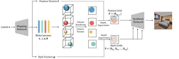
Figure 2: The architecture of the generator in BlobGAN-3D. A latent vector is fed into a mapping network to obtain the parameters of all the blobs. Given a camera pose, the blobs’ parameters are then used to compute the density for all the query points along the camera rays. We then use volume rendering to go from 3D density volumes to 2D density maps. The feature vectors and style vectors are then splatted on the density maps to get the corresponding grids, which serve as the input and condition for the synthesis network, respectively. The final RGB image is rendered by the synthesis network.

2.2 3D-aware GANs

Instead of directly synthesizing 2D images, 3D-aware GANs find an object’s or even whole scene’s 3D representation and derive 2D images from it. Given only single-view 2D images as input, voxel representations [19, 34] are used but they introduce large memory constraints. In contrast, neural fields are continuous and can synthesize images at arbitrary resolution. Neural fields are popular for 3D geometry processing tasks [10, 32, 40, 16, 7, 42, 58] and also enable 3D-aware image synthesis [37, 48, 38, 59]. NeRF [33, 67] combines the neural implicit network with differentiable volume rendering to enable explicit camera control for novel view image generation. Based on NeRF, GRAF [47], pi-GAN [8] and GRAM[12] propose to learn an implicit network to model the scene. GIRAFFE and GIRAFFE-HD [36, 61] learn a compositional neural field and enable object-level control. StyleNeRF [18] learns a low-dimensional feature map using NeRF and then progressively upsamples it to obtain the final RGB image. VolumeGAN [60] learns an extra convolutional structural representation as the coordinate descriptor for the mapping network. EG-3D [9] proposes an explicit-implicit tri-plane representation to combine efficiency and expressiveness. CIPS-3D [69] synthesizes images directly in a pixel-wise manner and enables convenient transfer learning tasks. MVCGAN [68] uses explicit multiview constraints to enhance multiview consistency over images. [51] builds a dual generator to take both RGB images and depth maps as input to help generate 3D indoor scene images. EpiGRAF [52] proposes a new patch-wise training scheme to efficiently obtain high-resolution images. However, most of these works only focus on the quality of the generated image and multiview consistency but are not aware of local multi-object editing in images. Some of the works [71, 34, 60, 53, 54] can enable local editing, but are only limited to the single object context.

2.3 Editability in GANs

For object-level editing, some works [71, 34, 60] can learn disentangled shape and appearance latent codes and enable independent control over the structure and texture. IDE-3D [53] and FENeRF [54] use semantic masks as an extra source of input to enable more local editing on human faces. However, some works [53, 54] only focus on face data, and require paired semantic mask labels as input. BlockGAN [35] computes a voxel feature grid for individual objects and successfully allows object-level control in a synthetic multiple-object scene [21]. Instead of using a voxel representation, GIRAFFE [36] learns multiple implicit fields for objects and also achieves good editing results on synthetic datasets. Liao et al. [30] propose 3D controllable image synthesis. Compared to our work, they use a differentiable projection layer rather than volume rendering, and use a 2D generator to render each object individually, rather than rendering a composite image. For BlockGAN, GIRAFFE and [30], when dealing with more complex real-world datasets like LSUN Bedroom [64], they struggle to generate high-quality images and synthesize poor multiview images. BlobGAN [14] uses a mid-level blob representation to model the scene and enables various local editing operations for individual objects in the scene on the challenging LSUN indoor datasets. It can move, remove, duplicate, swap, and re-stylize objects in the scene by manipulating the corresponding blobs. However, as a 2D GAN, BlobGAN ignores the 3D structure of the real-world scene, which limits its capability of editing. In this work, we extend BlobGAN to be 3D-aware, therefore allowing more control over editing while synthesizing novel-view images.

3 Method

Our method adopts the model architecture and design from BlobGAN [14]. Similarly, a random noise vector is fed into an MLP mapping network to obtain a representation of each blob. These representations are then mutually processed to get a joint feature grid, which is fed into a StyleGAN2-based synthesis network to generate images. Originally, the blobs are parameterized as ellipses, i.e. in 2D space. We extend the blobs to be modeled as 3-dimensional ellipsoids and colocate them in 3D scene space. We use volume rendering to go from 3D scene space to a 2D feature map and use a StyleGAN2 synthesis network to obtain the final RGB image. The architecture of the generator is shown in Fig. 2.

3.1 Extending from 2D space to 3D space

3.1.1 Blob parameterization

We model the whole scene as a 3-dimensional normalized coordinate system and use $M$ 3D blobs to represent its layout. We effectively double the number compared to BlobGAN and use 10 geometric parameters to define each blob $\{b_{i}\}_{i=1}^{M}$ by its center coordinate $\mathbf{x}_{i}\in\mathbb{R}^{3}$, scale factor $s_{i}\in\mathbb{R}$, normalized aspect ratio $\mathbf{a}_{i}\in\mathbb{R}^{3}$ and Euler rotation angles $\bm{\theta}_{i}\in\mathbb{R}^{3}$. We also learn a feature vector $\mathbf{f}_{i}\in\mathbb{R}^{d_{s}}$ and a style vector $\bm{\phi}_{i}\in\mathbb{R}^{d_{t}}$ to encode the structure and texture information per blob, where $d_{s}$ and $d_{t}$ are the dimensions of the feature vector and style vector, respectively.

3.1.2 Volume rendering

For a single pass, we assume a fixed camera pose to render all visible blobs. To obtain the density value at a query point $\mathbf{x}_{q}$ along a ray through the camera, we first calculate the squared Mahalanobis distance $d(\mathbf{x}_{q},\mathbf{x}_{i})$ between $\mathbf{x}_{q}$ and the blob center $\mathbf{x}_{i}$:

$$d(\mathbf{x}_{q},\mathbf{x}_{i})=(\mathbf{x}_{q}-\mathbf{x}_{i})^{T}(R_{i}\Sigma R_{i}^{T})^{-1}(\mathbf{x}_{q}-\mathbf{x}_{i}),$$ (1)

where $R_{i}$ is a $3\times 3$ rotation matrix computed by angles $\bm{\theta}_{i}$,

$$\Sigma=c\begin{pmatrix}a_{1}&0&0\\ 0&a_{2}&0\\ 0&0&a_{3}\end{pmatrix}$$ (2)

is a diagonal matrix with aspect ratio $\mathbf{a}_{i}$ along its diagonal and $c$ is a small scalar to control the sharpness of blob edges. We calculate the final density value at query point $\mathbf{x}_{q}$ w.r.t. blob center $\mathbf{x}_{i}$ by

$$\sigma(\mathbf{x}_{q},\mathbf{x}_{i})=\text{sigmoid}(s_{i}-d(\mathbf{x}_{q},\mathbf{x}_{i})),$$ (3)

where the sigmoid operation ensures a density value between 0 and 1, and the scale factor $s_{i}$ controls the size of the blob by adjusting the magnitude of density. For simplicity, we assume a clear ordering of all $M$ blobs along the depth axis, which is specified by their center position $\mathbf{x}_{i}$. This assumption implies that difficult blob intersections will not greatly influence the results and we therefore evaluate M density volumes independently.

While the density value changes depending on $\mathbf{x}_{q}$, we predefine the structure feature vector $\mathbf{f}_{i}$ representing the feature value of blob $b_{i}$ to stay constant, allowing us to derive $M$ spatially-invariant feature volumes in total. This is different than other 3D modeling designs, which obtain feature values depending on the query points. We justify this design choice by referring to the high memory consumption a spatially-variant feature volume computation would imply for our multi-blob layout. Moreover, we counteract a possible degradation of output quality by choosing $\mathbf{f}_{i}$ to consist of 768 features values, while other works doing spatially-variant computation usually only have 32. We follow the method in [33, 60] to render the density volume of blob $b_{i}$ in a front-to-back manner and choose $N$ sample points along each ray to compute the weighted feature vector $\mathbf{f}_{i}$ at a single pixel position $\mathbf{x}_{p}$ in feature map $\mathbf{M}_{i}$. Having a constant feature vector $\mathbf{f}_{i}$ per blob $b_{i}$ allows us to compute a scalar weight per pixel first and only performing a single multiplication per pixel afterwards by applying

$$\mathbf{M}_{i}(\mathbf{x}_{p})=O_{i}(\mathbf{x}_{p})\mathbf{f}_{i}$$ (4)

with

$$O_{i}(\mathbf{x}_{p})=\sum^{N}_{k=1}T_{k}(1-\exp(-\sigma_{k}\delta_{k}))$$ (5)

and

$$T_{k}=\exp(-\sum^{k-1}_{j=1}\sigma_{j}\delta_{j}),$$ (6)

where $O_{i}$ is the opacity map of $b_{i}$, $\delta_{k}=||\mathbf{x}_{k+1}-\mathbf{x}_{k}||_{2}$ is the distance between adjacent sample points, $\sigma_{k}=\sigma(\mathbf{x}_{k},\mathbf{x}_{i})$ denotes the density at sample point $\mathbf{x}_{k}$ w.r.t. blob center $\mathbf{x}_{i}$ and $T_{k}$ is a measure for the accumulated transmittance along the ray between $\mathbf{x}_{1}$ and $\mathbf{x}_{k}$.

3.1.3 Occlusions and foreshortening effect

BlobGAN [14] resolves occlusions between objects using alpha compositing [43] but only used the assigned index of each blob to identify the order. After training, changing this order is only possible by a permutation of indices. Since we also find a clear back-to-front ordering of blobs to do alpha compositing but explicitly model the depth, BlobGAN can be seen as a special case of our proposed method.

Specifically, given the camera intrinsics and extrinsics, we identify the direction of a ray traced through each pixel and calculate the depth of each blob in the camera coordinate system. In our approach, the depth order can naturally change in case the camera or the blobs are freely moved in space. After identifying the depth ordering of blobs along a ray, the vector-value at each pixel $x_{p}$ on the final feature grid $\mathbf{F}$ is given by:

$$\mathbf{F}(\mathbf{x}_{p})=\sum_{i=1}^{M}O_{i}(\mathbf{x}_{p})\left(\prod^{M}_{j=i+1}\left(1-O_{j}(\mathbf{x}_{p})\right)\right)\mathbf{f}_{i}.$$ (7)

We argue that the benefits of our 3D design are not only to give the users more freedom to determine occlusions, but we explicitly control the 3D location of objects during inference. More importantly, we apply a perspective projection from 3D to 2D, while recent work [14] only applies a parallel projection. In the latter case, there is no foreshortening effect in the generated images. Even when changing the implicit depth by permuting indices in BlobGAN, the projected object size will not vary because of the parallel projection, while in our method the size of the projection is inherently connected to the depth.

3.2 Image Generation

In BlobGAN, the resolution $L_{H}$ of the computed opacity map is chosen to be equal to the resolution of the output RGB image. Then $2\times$ downsampling is applied consecutively to get a sequence of opacity maps at lower resolutions $L_{1},L_{2},...,L_{H}$. BlobGAN replaces the constant input in the StyleGAN2 generator with the feature grid $\mathbf{F}$ at $L_{1}$ by splatting the feature vectors onto the opacity maps and then summing over these opacity maps. Also, the affine-transformed style vector which modulates the convolution weights in the StyleGAN2 generator block is replaced with a collection of hierarchical spatial-variant style grids $\mathbf{S}=\{\mathbf{S}_{L_{1}},\mathbf{S}_{L_{2}},...,\mathbf{S}_{L_{H}}\}$. Specifically, they splat the opacity maps of hierarchical spatial resolutions with style vectors $\bm{\phi}_{i}$ to get the style grids of hierarchical spatial resolutions. They do a per-pixel affine transformation on the normalized style grid and then multiply it with the input feature grid before applying the normalized convolutional operator. As in StyleGAN2, the low spatial resolution input feature grid is transformed into a high-resolution RGB image by a sequence of convolutional upsampling blocks. For each feature grid at a certain resolution, a style grid of the same spatial resolution controls the modulation of the corresponding convolutional block. In BlobGAN, to output a $L_{H}\times L_{H}$ RGB image, they compute the opacity map at a resolution of $L_{H}\times L_{H}$. However, we find that instead of computing each opacity map at $L_{H}\times L_{H}$, we advocate directly computing it at a lower resolution. We choose $L_{H-1}\times L_{H-1}$ to find a balance between detail preservation and computational efficiency. For the remaining lower-resolution opacity maps, we keep using downsampling; for the higher-resolution opacity maps, e.g. $L_{H}\times L_{H}$, we design an upsampling block to obtain them.

Given input $X\in R^{H\times W\times C}$, to obtain the output $X_{\text{up}}\in R^{2H\times 2W\times C}$, we have:

$$X_{\text{up}}=\text{Bilinear}(X)+\text{PixelShuffle}(\text{ModConv}(X)),$$ (8)

where ModConv is a $1\times 1$ convolution modulated by the feature vector of each blob, PixelShuffle is an upsampling operator proposed in [50]. We initialize the weight of the ModConv to $0$, such that the upsampling block reduces to a bilinear operator at the beginning. In fact, in 3D image synthesis tasks, it could be very expensive to directly compute the opacity maps $O=\{O_{1},O_{2},...,O_{M}\}$ at $L_{H}\times L_{H}$ as in BlobGAN, which means we have to do volume rendering at $L_{H}\times L_{H}$ to obtain the feature maps $\mathbf{M}=\{\mathbf{M}_{1},\mathbf{M}_{2},...,\mathbf{M}_{M}\}$. As the third dimension is modeled, we have to decrease the spatial resolution of the volume rendering step to save memory. The difference between the computation of the hierarchical opacity maps in BlobGAN and BlobGAN-3D and the design of the upsampler module are shown in the supplementary materials.

3.3 Multiview Control

3.3.1 Viewpoint disentanglement in StyleGAN2

As demonstrated in [20, 29, 1, 56], StyleGAN2 can disentangle viewpoints in the early layers. Also, as is the design in BlobGAN, the input feature grid of the generator is at a low resolution of $L_{1}\times L_{1}$, which could lead to a loss of spatial details when doing the upsampling to obtain the final $L_{H}\times L_{H}$ RGB image. In a 3D-aware setting, this loss may also cause multiview inconsistency. Therefore, to get a better multiview consistency effect, we add a skip connection of the input to the output of the first two convolutional blocks in the synthesis network. We find this can help multiview consistency to some extent, but there is still room for improvement. We subsequently use depth supervision to enhance the multiview consistency.

3.3.2 Depth supervision

Unlike other 3D-aware image synthesis networks, where the scene is modeled as a whole, blobs decompose the scene into different parts. This blob design brings extra challenges in multiview rendering. In BlobGAN-3D, when moving the camera, all the blobs rendered in the image will move at the same time, compared to the blob-level editing where only one or at most several blobs are moving at the same time. It is much more challenging to render a realistic scene when all the blobs can appear in different locations on the image plane, as once the depths of some blobs in 3D space are wrong, they may unexpectedly occlude other blobs when moving, resulting in multiview inconsistency and other artifacts. Thus, it is critical to correctly model the depths of the blobs to have good multiview consistency. We find that it could be hard for the network to optimize the depths for all the blobs in an unsupervised way. So, we include an off-the-shelf pre-trained depth estimation network to help the network correct the depth it learns for each blob. We apply an extra MSE loss $l_{\text{depth}}$ between the learned depth of the centroid of each blob and the predicted depth of that centroid projected onto the image using the depth estimator. In detail, for the blob centroid $(x_{s},y_{s},z_{s})$ in the world coordinate, which is projected to the location $(u,v)$ on the image, we have:

$$l_{\text{depth}}=||z_{s}-D(u,v)||^{2},$$ (9)

where $D$ is the depth estimator. We also find that it is not helpful to start training with the multiview rendering unless the learned depths of the blobs are correct. Thus, we employ a two-stage training strategy:

1. Fixing the camera pose as front-view, training the network until it reaches a good texture quality.

2. Applying the depth estimator to correct the depths of the blob centroids while rendering the image from a randomly sampled camera pose.

4 Experiments

Table 1: Comparison between BlobGAN and our method. Our method not only enables object-evel editing in BlobGAN, but also enables additional 3D effects which do not exist in BlobGAN.

	Moving	Resizing	Reshaping	Restyling	Multiview	Depth control	Foreshortening
BlobGAN	✓	✓	✓	✓	✗	✗	✗
Ours	✓	✓	✓	✓	✓	✓	✓

Table 2: Comparison of disentanglement properties. Our method is 3D aware and also object-level disentangled. Fg/Bg means the method can disentangle foreground and background, but cannot further disentangle individual objects. Objects means the method can disentangle individual objects.

	3D-aware	Disentang.	Disentang. level
GIRAFFE	✓	✓	Objects
VolumeGAN	✓	✗	–
StyleNeRF	✓	✓	Fg/Bg
EG3D	✓	✗	–
BlobGAN	✗	✓	Objects
Ours	✓	✓	Objects

4.1 Settings

Dataset.

We use two indoor multi-object scene datasets, Bedroom and Conference room, from LSUN [64] to evaluate our model. The datasets contain $3$M and $200$K images, respectively. We train at $256\times 256$ resolution.

Baselines.

We compare our method with BlobGAN[14], GIRAFFE[36], VolumeGAN[60], StyleNeRF[18] ,and EG3D[9]. We build our implementation on top of BlobGAN. The differences between BlobGAN and BlobGAN-3D are shown in Tab. 1. GIRAFFE is a 3D-aware GAN with multi-object editing capabilities on synthetic datasets. VolumeGAN, StyleNeRF and EG3D are 3D-aware GANs without multi-object editability. A comparison of the properties of our method and the baselines is shown in Tab. 2.

Metric.

We use FID and KID [4]. We use $50$K real images and $50$K fake images to compute both FID and KID using the method proposed in [41].

Implementation details.

For both datasets, we empirically identified a suitable number of blobs $M=10$. A smaller number results in the decrease of quality, while a larger number implicates a higher computational complexity. The output image resolution is $L_{H}\times L_{H}=256\times 256$. We perform volume rendering at $L_{H-1}\times L_{H-1}=128\times 128$. The resolution of the feature grid we feed into the synthesis network is $L_{1}\times L_{1}=16\times 16$. The off-the-shelf depth estimator we adopt is from [44]. We randomly sample $32$ points along each ray of the camera. More details can be found in Supplementary materials.

Table 3: Quantitative results of image quality on two datasets. Our method achieves good image quality compared to the 3D GAN baselines and BlobGAN.

	Bedroom		Conference room
	FID $\downarrow$	KID $\downarrow$	FID $\downarrow$	KID $\downarrow$
GIRAFFE	49.62	0.046	73.99	0.066
VolumeGAN	17.3	–	43.92	0.032
StyleNeRF	13.50	0.011	23.09	0.018
EG3D	10.25	0.0071	15.08	0.0099
Ours	4.16	0.0023	7.80	0.0039
BlobGAN	3.76	0.0021	6.76	0.0033
BlobGAN ($25000$K)	11.5	0.0084	11.01	0.0064
Ours ($25000$K)	11.7	0.0096	15.38	0.0100

Table 4: FID after editing the scene. # blobs means the number of the blobs being moved. We randomly choose which blobs to move and move them by 0.2 in normalized coordinate space in the horizontal direction.

	Bedroom			Conf. room
# blobs	1	3	5	1	3	5
BlobGAN	4.04	4.24	4.68	6.94	7.22	7.61
Ours	4.11	4.13	4.23	7.80	8.09	8.24

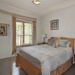
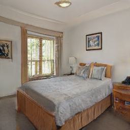
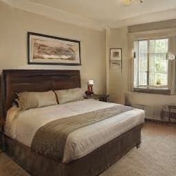
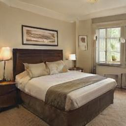
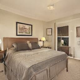
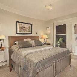
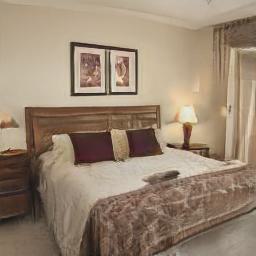
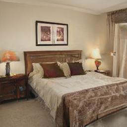
Figure 3: Foreshortening effect. By adjusting the horizontal position and the depth of the blob at the same time, we achieve a foreshortening effect: when the bed is moving away from the camera, its size in the image becomes smaller.

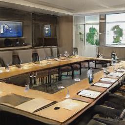
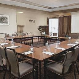
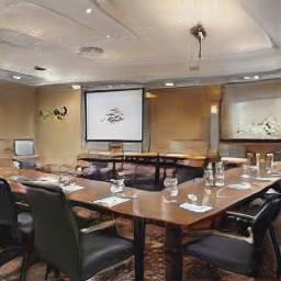
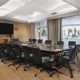
\begin{overpic}[width=496.85625pt]{figures/editing/moving/bedroom_blob_0.jpg} \put(35.0,30.0){\color[rgb]{1,1,1}\vector(1,0){40.0}} \end{overpic}

\begin{overpic}[width=496.85625pt]{figures/editing/moving/bedroom_blob_2.jpg} \put(55.0,30.0){\color[rgb]{1,1,1}\vector(1,0){40.0}} \end{overpic}

\begin{overpic}[width=496.85625pt]{figures/editing/moving/bedroom_blob_4.jpg} \put(77.0,68.0){\color[rgb]{1,1,1}\vector(1,0){25.0}} \end{overpic}

\begin{overpic}[width=496.85625pt]{figures/editing/moving/bedroom_blob_6.jpg} \put(67.0,72.0){\color[rgb]{1,1,1}\vector(1,0){30.0}} \end{overpic}

\begin{overpic}[width=496.85625pt]{figures/editing/moving/conference_blob_0.jpg} \put(71.0,21.0){\color[rgb]{1,1,1}\vector(1,0){30.0}} \end{overpic}

\begin{overpic}[width=496.85625pt]{figures/editing/moving/conference_blob_2.jpg} \put(58.0,21.0){\color[rgb]{1,1,1}\vector(1,0){30.0}} \end{overpic}

\begin{overpic}[width=496.85625pt]{figures/editing/moving/conference_blob_4.jpg} \put(40.0,58.0){\color[rgb]{1,1,1}\vector(1,0){30.0}} \end{overpic}

\begin{overpic}[width=496.85625pt]{figures/editing/moving/conference_blob_6.jpg} \put(48.0,70.0){\color[rgb]{1,1,1}\vector(1,0){30.0}} \end{overpic}

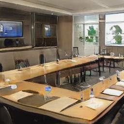
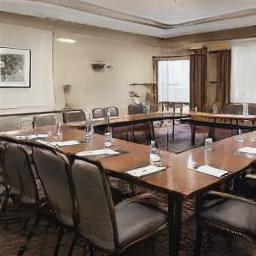
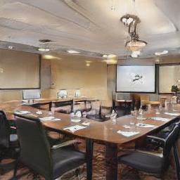
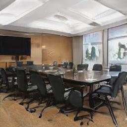
Figure 4: Moving an object in the scene. The first row shows the original generated images; the second row shows the corresponding blob layout maps with marks demonstrating the moving direction. The last row shows the synthesized images after moving one blob.

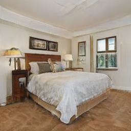
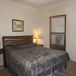
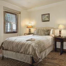
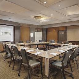
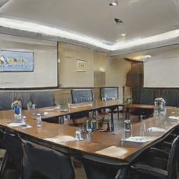
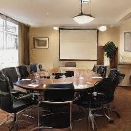
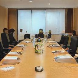
\begin{overpic}[width=496.85625pt]{figures/editing/resizing/bedroom_blob_0.jpg} \put(38.0,40.0){\color[rgb]{1,1,1}\line(1,-1){20.0}} \put(58.0,40.0){\color[rgb]{1,1,1}\line(-1,-1){20.0}} \end{overpic}

\begin{overpic}[width=496.85625pt]{figures/editing/resizing/bedroom_blob_2.jpg} \put(43.0,40.0){\color[rgb]{1,1,1}\line(1,-1){20.0}} \put(63.0,40.0){\color[rgb]{1,1,1}\line(-1,-1){20.0}} \end{overpic}

\begin{overpic}[width=496.85625pt]{figures/editing/resizing/bedroom_blob_4.jpg} \put(66.0,70.0){\color[rgb]{1,1,1}\line(1,-1){15.0}} \put(81.0,70.0){\color[rgb]{1,1,1}\line(-1,-1){15.0}} \end{overpic}

\begin{overpic}[width=496.85625pt]{figures/editing/resizing/bedroom_blob_6.jpg} \put(62.0,77.0){\color[rgb]{1,1,1}\line(1,-1){15.0}} \put(77.0,77.0){\color[rgb]{1,1,1}\line(-1,-1){15.0}} \end{overpic}

\begin{overpic}[width=496.85625pt]{figures/editing/resizing/conference_blob_0.jpg} \put(35.0,40.0){\color[rgb]{1,1,1}\line(1,-1){30.0}} \put(63.0,40.0){\color[rgb]{1,1,1}\line(-1,-1){30.0}} \end{overpic}

\begin{overpic}[width=496.85625pt]{figures/editing/resizing/conference_blob_2.jpg} \put(38.0,32.0){\color[rgb]{1,1,1}\line(1,-1){28.0}} \put(64.0,32.0){\color[rgb]{1,1,1}\line(-1,-1){28.0}} \end{overpic}

\begin{overpic}[width=496.85625pt]{figures/editing/resizing/conference_blob_4.jpg} \put(48.0,78.0){\color[rgb]{1,1,1}\line(1,-1){20.0}} \put(68.0,78.0){\color[rgb]{1,1,1}\line(-1,-1){20.0}} \end{overpic}

\begin{overpic}[width=496.85625pt]{figures/editing/resizing/conference_blob_6.jpg} \put(28.0,72.0){\color[rgb]{1,1,1}\line(1,-1){20.0}} \put(48.0,72.0){\color[rgb]{1,1,1}\line(-1,-1){20.0}} \end{overpic}

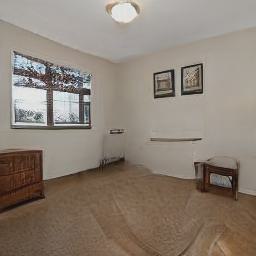
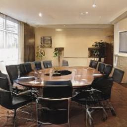
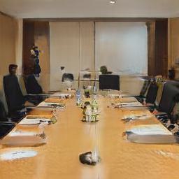
Figure 5: Removing an object in the scene. The first row shows the originally generated images; the second row shows the corresponding blob layout maps with marks demonstrating the removed blob. The last row shows the synthesized images after removing one blob.

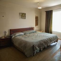
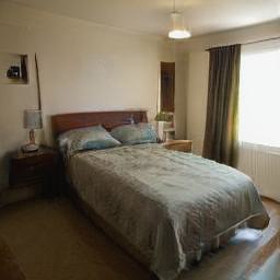
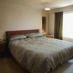
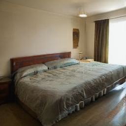
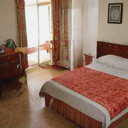
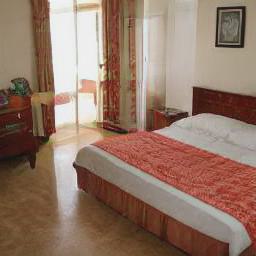
Figure 6: Changing the aspect ratio of the blobs. Different shapes of the blobs are obtained by changing the aspect ratio of the blob which represents the bedroom.

GIRAFFE

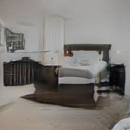
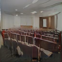
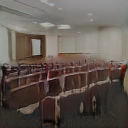
VolumeGAN

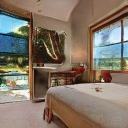
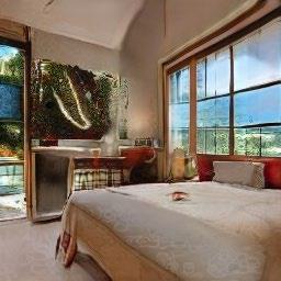
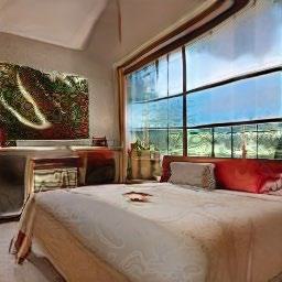
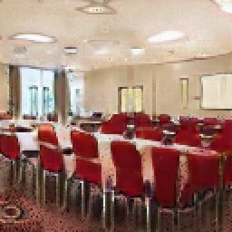
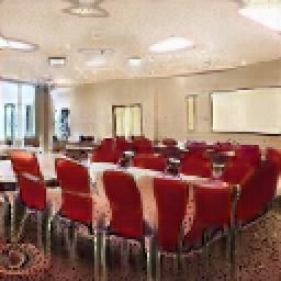
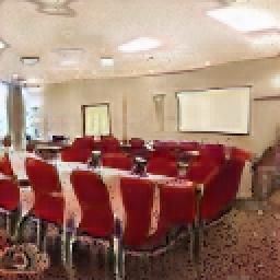
StyleNeRF

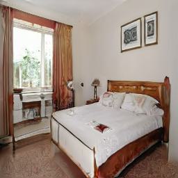
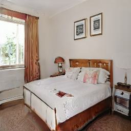
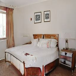
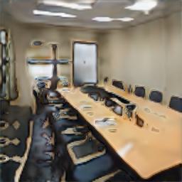
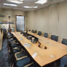
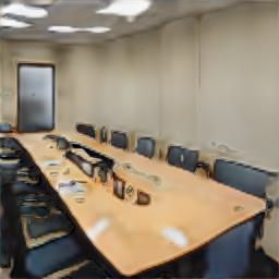
EG3D

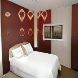
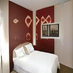
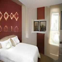
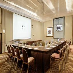
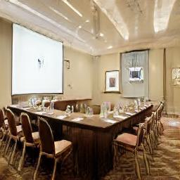
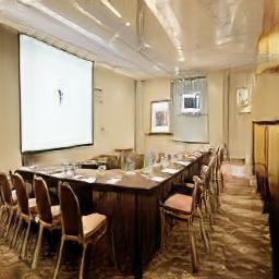
Ours

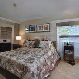
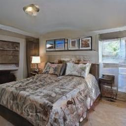
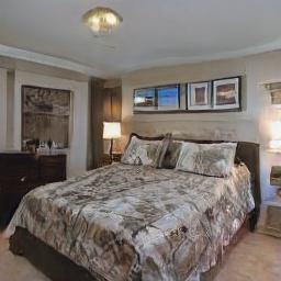
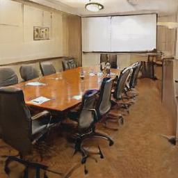
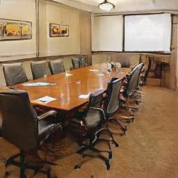
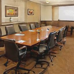
Ours

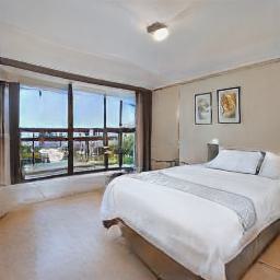
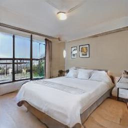
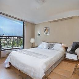
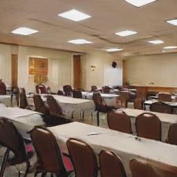
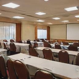
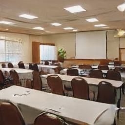
Figure 7: Multiview image synthesis results. The results of VolumeGAN on the Bedroom dataset are borrowed from [60]. We disable the camera pose conditioning in EG3D as it is difficult to estimate camera poses for indoor datasets.

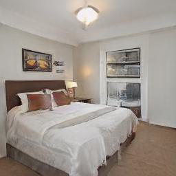
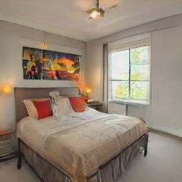
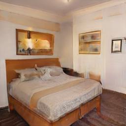
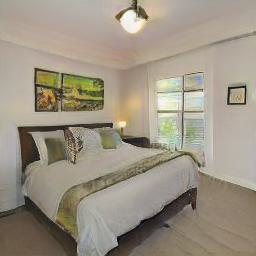
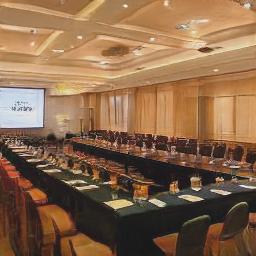
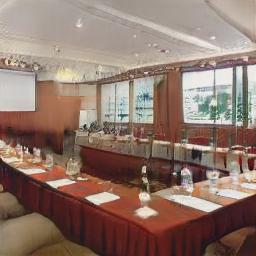
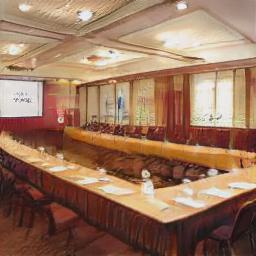
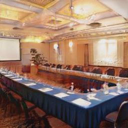
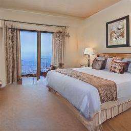
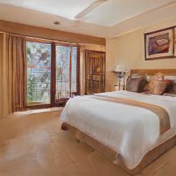
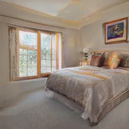
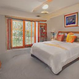
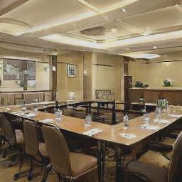
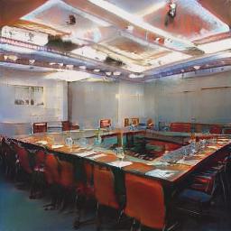
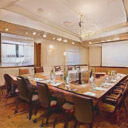
Figure 8: Restyling of the scene. In each row we show different decorating styles of the same bedroom or conference room by simply swapping different style vectors $\bm{\phi}_{i}$ for all the blobs.

4.2 Quantitative results

We show the quantitative results of our method and baselines in Tab. 3. Our method achieves comparable quality against 2D BlobGAN and 3D-aware baselines. We also provide the results of BlobGAN and our method when training for $25000$K images for a fair comparison.

For evaluating the quality of synthesized images after editing, we provide the FID evaluation of moving the objects in the scene in Tab. 4. It is interesting to see that BlobGAN-3D is relatively more stable to the editings than BlobGAN.

4.3 Qualitative results

4.3.1 Multiview rendering

We show the qualitative comparison of multiview rendering between our method and baselines in Fig. 7. Our method can achieve high image quality by synthesizing more realistic texture and fewer artifacts compared to the 3D-aware GAN baselines.

4.3.2 Scene editing

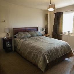
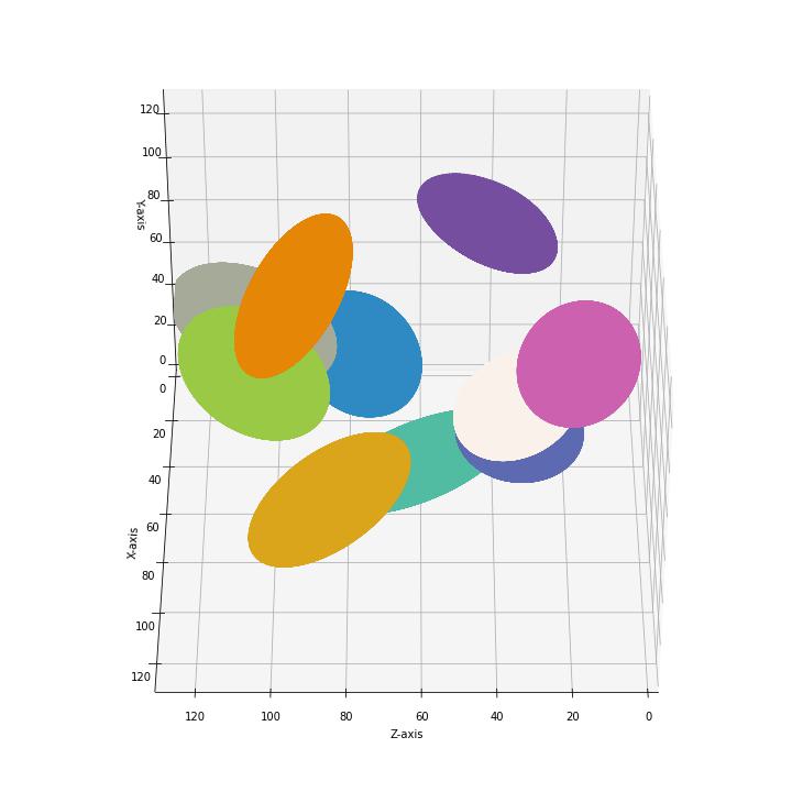
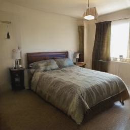
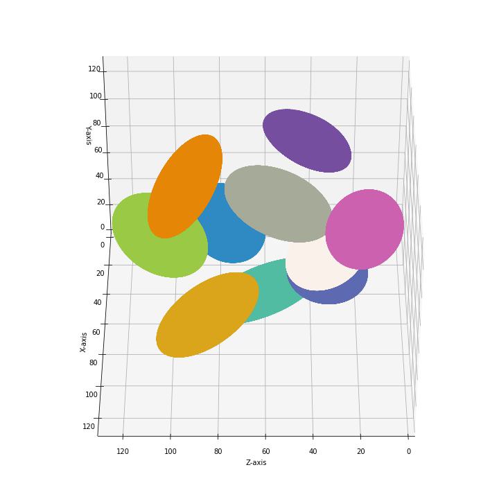
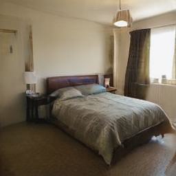
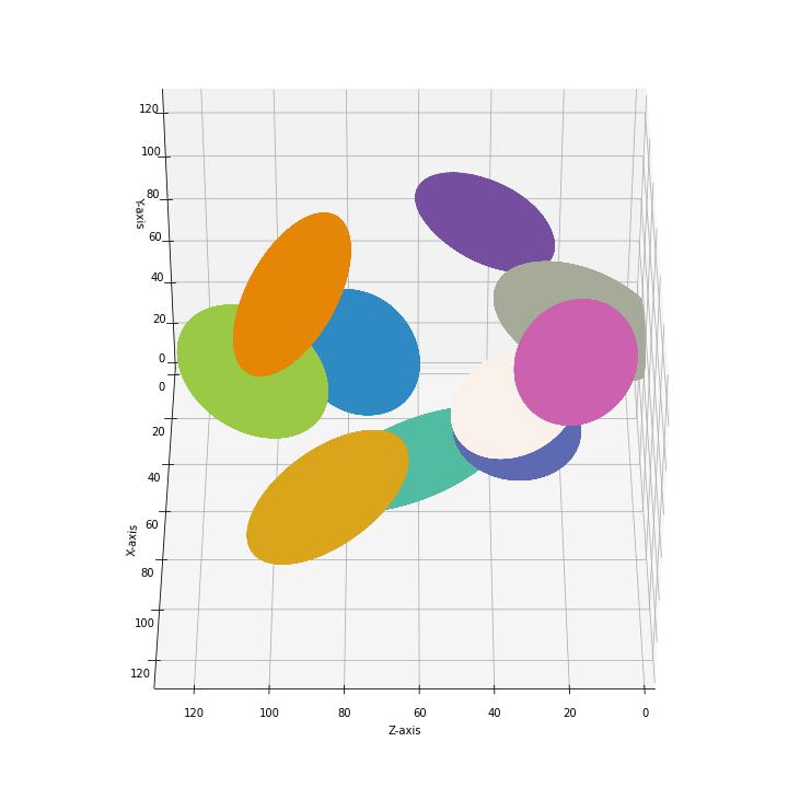
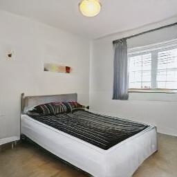
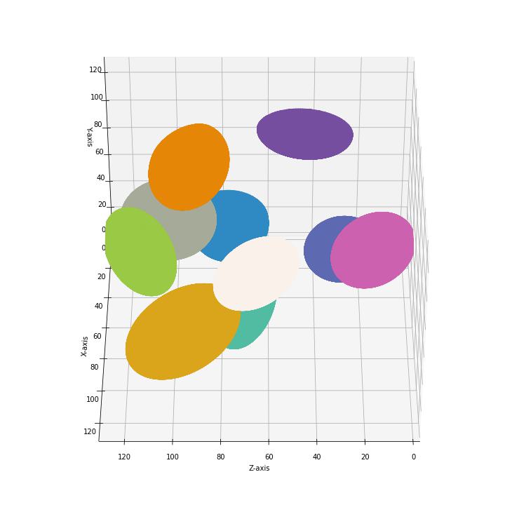
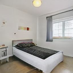
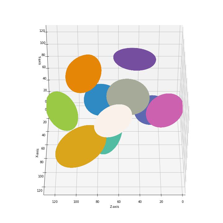
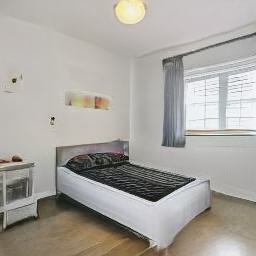
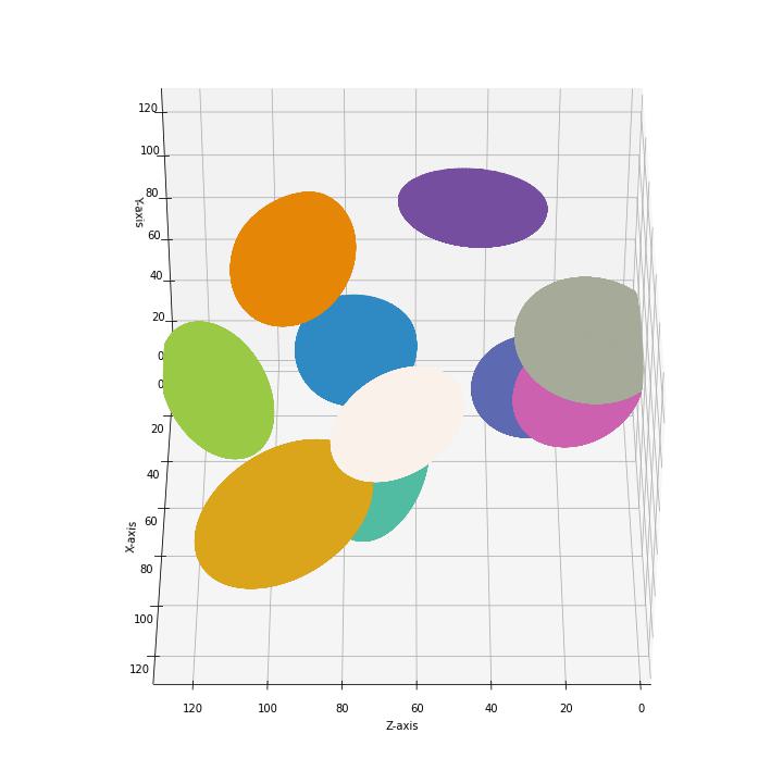
Figure 17: Foreshortening effect. When moving the gray blob which represents the bed along the depth dimension (Z-axis) away from the viewpoint, the size of the bed becomes smaller.

We show the scene editing results of moving (Fig. 12), removing (Fig. 14) and restyling (Fig. 8). More editing results can be found in the supplementary materials. We show that our method can disentangle individual objects in the scene to apply precise edits. Despite some minor changes, most of the other objects appearing in the scene remain the same after editing while the scenes still look realistic. We additionally show the results of changing the three aspect ratio values of the blobs in Fig. 6 and the foreshortening effect in Fig. 17.

5 Conclusions

In this work, we extend 2D GAN BlobGAN to be 3D-aware while keeping the disentanglement of the objects and can perform realistic object-level editing on complex real-world indoor datasets. We show that our model can achieve comparable image quality to the original BlobGAN and other 3D-aware GANs. Meanwhile, our method can achieve good multiview consistency while enabling object-level editing as done in BlobGAN. We also allow more editing capabilities by explicitly controlling the 3D location of the blobs in the scene and achieving a foreshortening effect.

Appendix A More implementation details

A.1 Upsampler

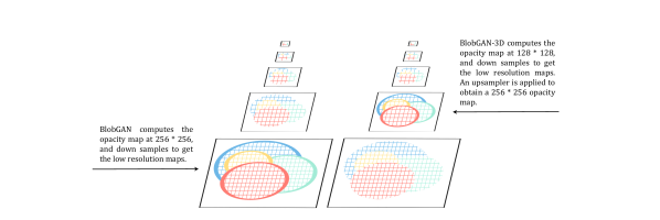
Figure 9: The difference between BlobGAN and BlobGAN-3D on how the hierarchical opacity maps are computed (left) and the designed upsampler module (right). In BlobGAN-3D, an additional upsampler module is applied to upsample the computed opacity map from $128\times 128$ to $256\times 256$.

We show the difference between BlobGAN and our BlobGAN-3D on how the hierarchical opacity maps are computed in Fig. 9 (left). In Fig. 9 (right), the architecture of the upsampler module is shown. We find the balance between computational complexity and performance by computing the opacity map at a resolution of $128\times 128$.

A.2 Additional training design

During the third training stage, in each iteration we randomly drop one blob with a probability of 0.5 when rendering the images. By doing this we want the network to synthesize realistic images even when an object disappears in the scene, which in turn can improve the disentanglement. When determining the occlusions, we initially forced the network to learn the depth of all blobs in descending order. This however is not helpful because it constrains the learning ability of the MLP network. We later allow the network to learn an arbitrary normalized depth for each blob followed by a sorting operation.

A.3 Training time and hyperparameters

Compared to other models which directly model the scene as a whole, BlobGAN and BlobGAN-3D suffer from a low convergence rate because the image rendering takes place on the feature grid of the blob representation instead of the scene representation. Originally, BlobGAN trained their models for 1.5 million gradient steps on 8 NVIDIA A100 GPUs for 4 weeks. This is roughly equal to a $288000$K-image training run. Due to the limited resources, we trained our model for around $200000$K images on each dataset on 4 NVIDIA A100 GPUs, compared to $25000$K images for other baselines. We use a per-GPU batch size of $16$.

For most of the settings, we follow BlobGAN. We use AdamW [31] optimizer with $\beta_{0}=0$ and $\beta_{1}=0.99$. We also use an exponentially moving average of the network weights [63] with a decay of $0.998$ as it was used in BlobGAN. For the mapping network, we use an $8$-layer $1280$-channel MLP compared to an $8$-layer $1024$-channel MLP in BlobGAN.

A.4 Volume rendering

Compared to Nerf-like volume rendering, we do not represent the volume as implicit function and do not use an MLP to query the density value and feature value. We instead use a squared Mahalanobis distance to compute the density at each query point in 3D space. This is similar to BlobGAN where an opacity value is computed at each query point in 2D space. We reuse the feature vector of each blob as feature value. The Mahalanobis distance computes the distance from a point to a distribution. We model the density of each blob as a normal distribution and choose a suitable parameterization. The closer a query point is to the center of the blob, the higher is the density value. Therefore, the density is a continuous value and can be computed at any given point. As the density of each location is closely related to the distance to the center of the blob, when the blob is moving, the density at each location will change accordingly.

Appendix B Qualitative results

We use the truncation technique similar to BlobGAN to improve the image quality. For all the figures in the paper, we use a truncation weight $w=0.6$. The truncation weight $w$ ranges from $0$ to $1$. The higher the truncation weight, the higher the image quality but the lower the diversity. To show the diversity of our generated images, we provide samples in Fig. 10 and Fig. 11 using $w=0.3$.

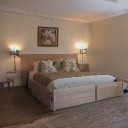
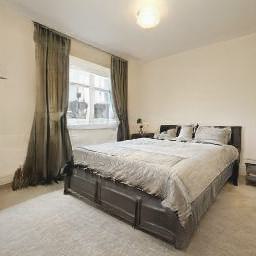
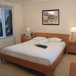
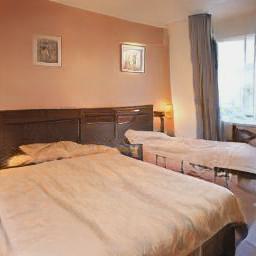
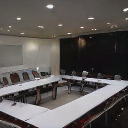
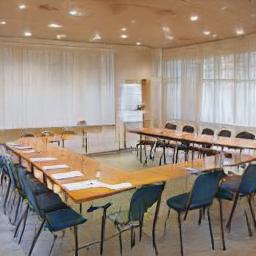
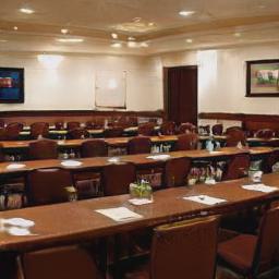
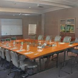
\begin{overpic}[width=496.85625pt]{figures_sup/2d/resizing/bedroom_blob_0.jpg} \put(45.0,45.0){\color[rgb]{1,1,1}\line(1,-1){20.0}} \put(65.0,45.0){\color[rgb]{1,1,1}\line(-1,-1){20.0}} \end{overpic}

\begin{overpic}[width=496.85625pt]{figures_sup/2d/resizing/bedroom_blob_2.jpg} \put(48.0,38.0){\color[rgb]{1,1,1}\line(1,-1){20.0}} \put(68.0,38.0){\color[rgb]{1,1,1}\line(-1,-1){20.0}} \end{overpic}

\begin{overpic}[width=496.85625pt]{figures_sup/2d/resizing/bedroom_blob_4.jpg} \put(60.0,74.0){\color[rgb]{1,1,1}\line(1,-1){15.0}} \put(75.0,74.0){\color[rgb]{1,1,1}\line(-1,-1){15.0}} \end{overpic}

\begin{overpic}[width=496.85625pt]{figures_sup/2d/resizing/bedroom_blob_6.jpg} \put(80.0,79.0){\color[rgb]{1,1,1}\line(1,-1){15.0}} \put(95.0,79.0){\color[rgb]{1,1,1}\line(-1,-1){15.0}} \end{overpic}

\begin{overpic}[width=496.85625pt]{figures_sup/2d/resizing/conference_blob_0.jpg} \put(35.0,35.0){\color[rgb]{1,1,1}\line(1,-1){30.0}} \put(63.0,35.0){\color[rgb]{1,1,1}\line(-1,-1){30.0}} \end{overpic}

\begin{overpic}[width=496.85625pt]{figures_sup/2d/resizing/conference_blob_2.jpg} \put(38.0,38.0){\color[rgb]{1,1,1}\line(1,-1){28.0}} \put(64.0,38.0){\color[rgb]{1,1,1}\line(-1,-1){28.0}} \end{overpic}

\begin{overpic}[width=496.85625pt]{figures_sup/2d/resizing/conference_blob_4.jpg} \put(48.0,78.0){\color[rgb]{1,1,1}\line(1,-1){20.0}} \put(68.0,78.0){\color[rgb]{1,1,1}\line(-1,-1){20.0}} \end{overpic}

\begin{overpic}[width=496.85625pt]{figures_sup/2d/resizing/conference_blob_6.jpg} \put(68.0,76.0){\color[rgb]{1,1,1}\line(1,-1){20.0}} \put(88.0,76.0){\color[rgb]{1,1,1}\line(-1,-1){20.0}} \end{overpic}

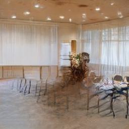
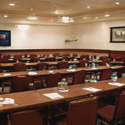
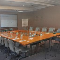
Figure 15: Original BlobGAN: Removing an object in the scene. The first row shows the originally generated images; the second row shows the corresponding blob layout maps with marks demonstrating the removed blob. The last row shows the synthesized images after removing one blob. We show these as a comparison to BlobGAN-3D.

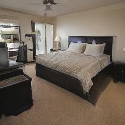
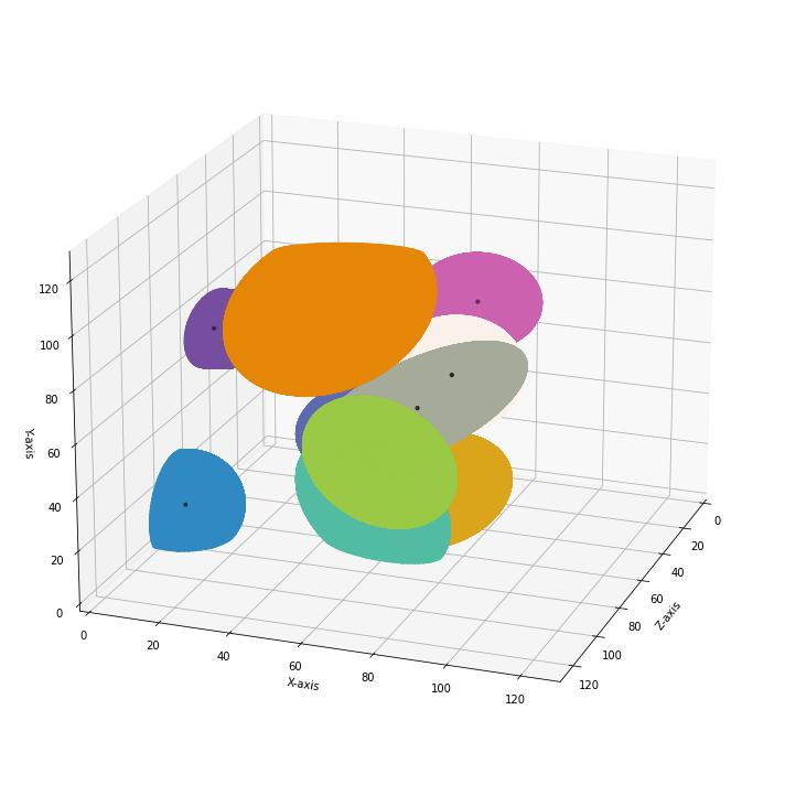
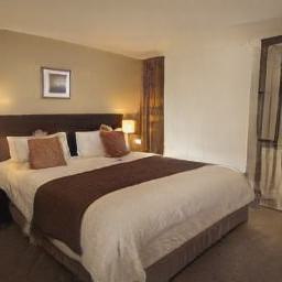
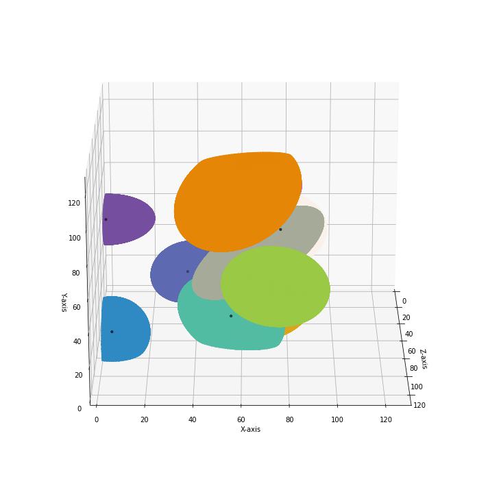
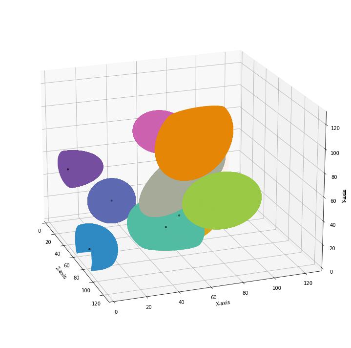
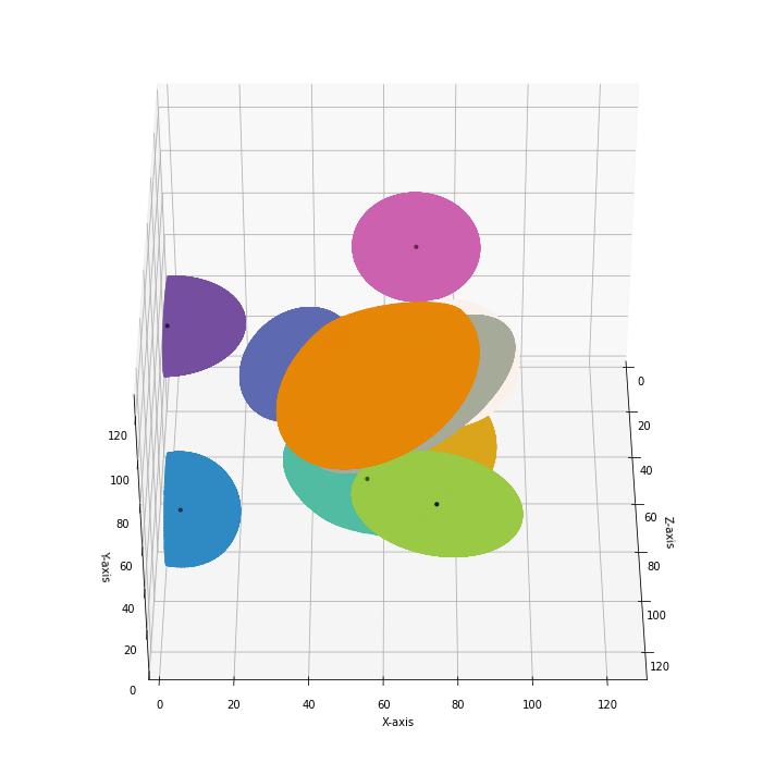
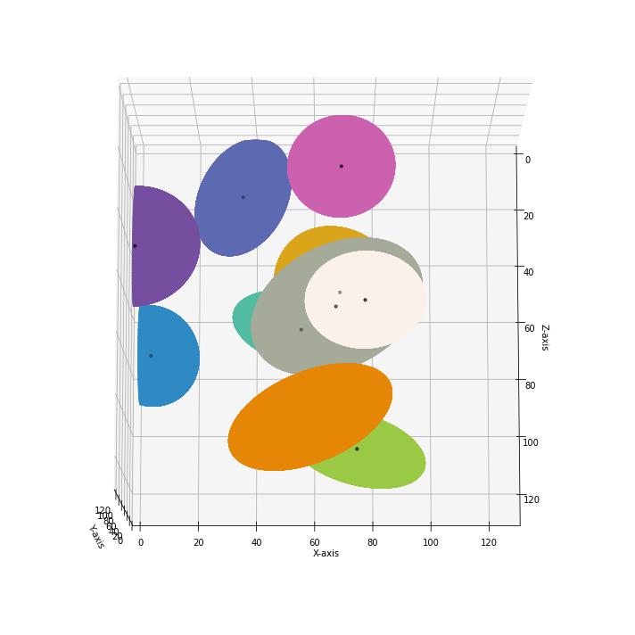
Figure 16: Blobs visualization in 3D space. The first column shows the synthetic image, the second to sixth column shows the corresponding blobs in 3D space which are visualized under different camera viewpoints.

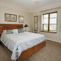
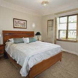
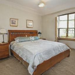
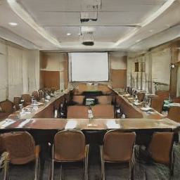
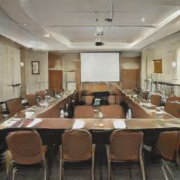
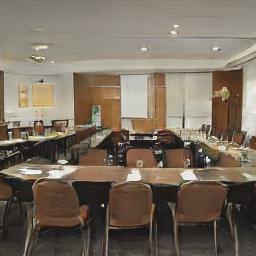
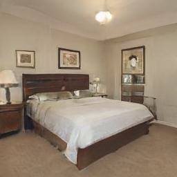
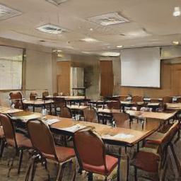
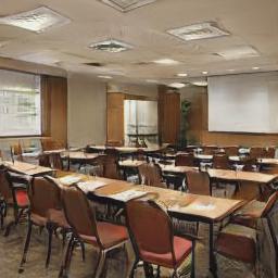
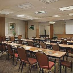
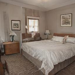
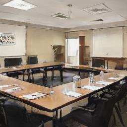
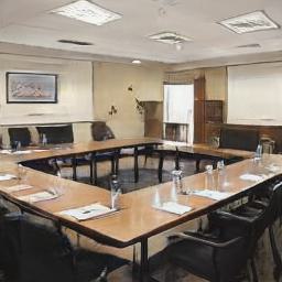
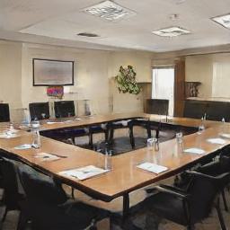
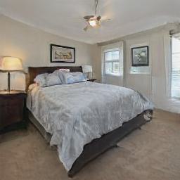
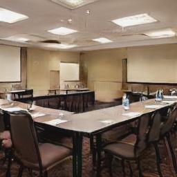
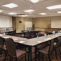
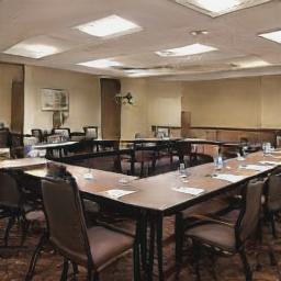
Figure 18: Moving the camera in the horizontal direction. For every two rows, the first row shows the generated images, while the second row shows the corresponding blobs layout map.

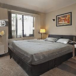
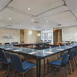
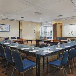
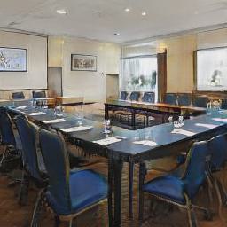
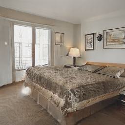
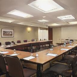
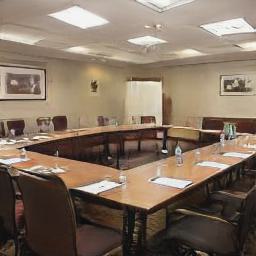
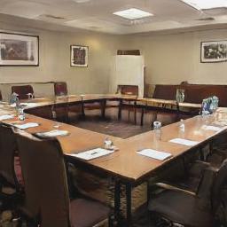
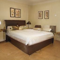
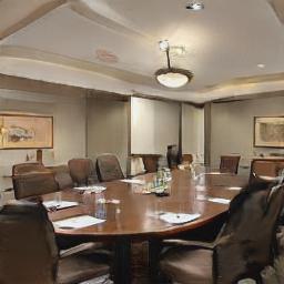
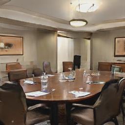
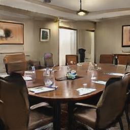
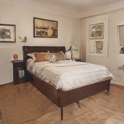
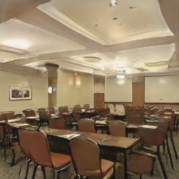
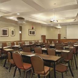
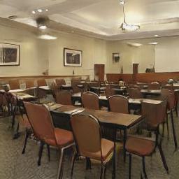
Figure 19: Moving the camera in the vertical direction. For every two rows, the first row shows the generated images, while the second row shows the corresponding blobs layout map.

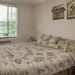
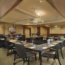
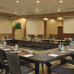
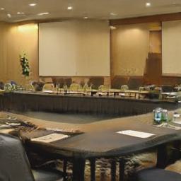
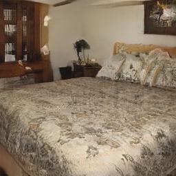
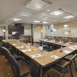
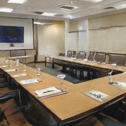
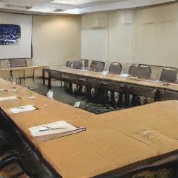
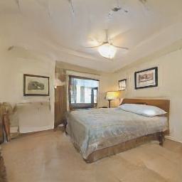
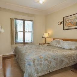
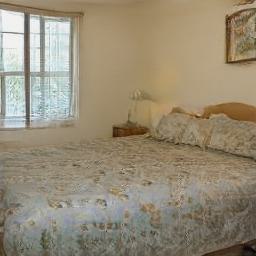
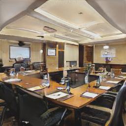
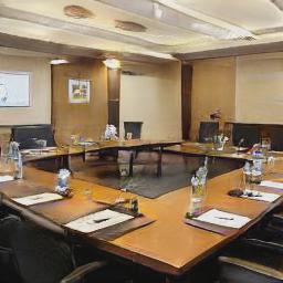
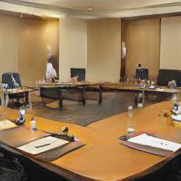
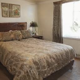
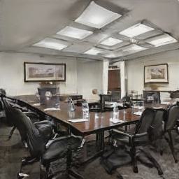
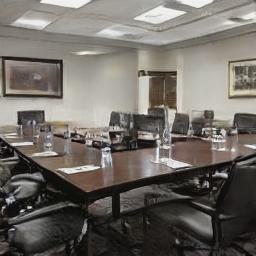
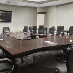
Figure 20: Moving the camera to simulate zoom in and zoom out effects. For every two rows, the first row shows the generated images, while the second row shows the corresponding blobs layout map.

We provide more editing results of moving objects in Fig. 12 and resizing objects in Fig. 14. For comparison, we show the editing results of original BlobGAN in Fig. 13 and Fig. 15. We visualize the blobs in 3D space in Fig. 16. In Fig. 17, we show more examples of the foreshortening effect along with the blob visualization in 3D space. We also show more qualitative results of multiview rendering by moving the camera in the horizontal direction (Fig. 18), vertical direction (Fig. 19) and closer to or away from the viewpoint (Fig. 20). Despite some minor changes due to the entanglement, our method achieves good consistency while enabling realistic multi-object editing on real-world indoor datasets.

Appendix C Ablation study

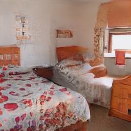
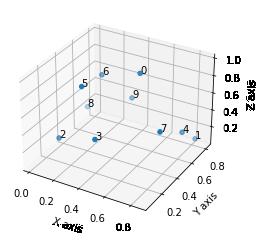
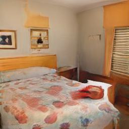
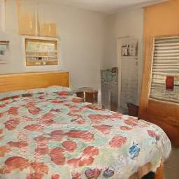
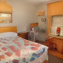
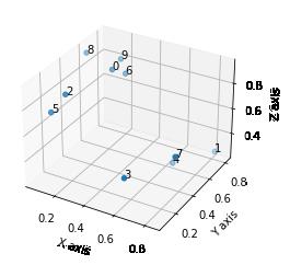
Figure 21: Depth supervision ablation study. The first row shows the results without depth supervision, while the second shows the results with depth supervision. The first three columns shows the results of multiview rendering. The fourth column shows the coordinates of all the blobs’ centers. With depth supervision, the image quality and the multiview rendering quality are better than without depth supervision.

We provide the results of an ablation study on depth supervision in Fig. 21. Because of limited resources, both models with and without depth supervision are not trained till convergence but for roughly the same number of iterations. We can also compute the same depth estimation loss as we defined before:

$$l_{\text{depth}}=||z_{s}-D(u,v)||^{2},$$ (10)

where $(x_{s},y_{s},z_{s})$ are the world coordinates of the blob center, $(u,v)$ are the coordinates of the projection in image space, and $D$ is the depth estimator. We randomly generate 5000 images under the same camera sampling strategy for each model and compute the corresponding depth estimation loss. Without depth supervision, the average depth estimation loss is 0.197. With depth supervision, this number drops around 36% to 0.116.

Appendix D Limitations

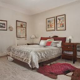
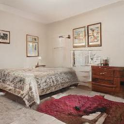
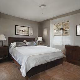
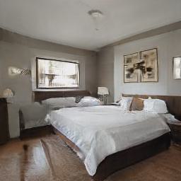
Figure 22: Typical failure cases in our method. When moving the bed in the scene, sometimes the original bedside will disappear, either because of being occluded by the painting blob above the bed, or the bedside is actually part of the painting blob above. A new bedside may appear on the other side of the bed, which is actually due to the failed disentanglement of the other painting blob.

Our work also has several limitations. Both BlobGAN and our work can obtain good disentanglement of individual objects in an unsupervised manner on a complex dataset. However, in both methods, the disentanglement is not perfect. Changing one blob may still influence the appearance or location of other objects in the scene. We show some typical failure cases in our method in Fig. 22. The depth estimator can help to correct the depth of the centroid of the blob. However, as the shape and size of the blobs are not perfectly matched to the shape and size of the corresponding object, the estimated depth from image space may not reveal the depth of the object in 3D scene. Despite good image quality, the time BlobGAN and BlobGAN-3D take to converge is very long compared to other GANs. We explain this long training time by the fact that the scene is modeled as a collection of blobs, which can be considered as an intermediate representation. Rendering the blobs first and mapping them to an image of the scene takes longer than just rendering the scene itself directly.

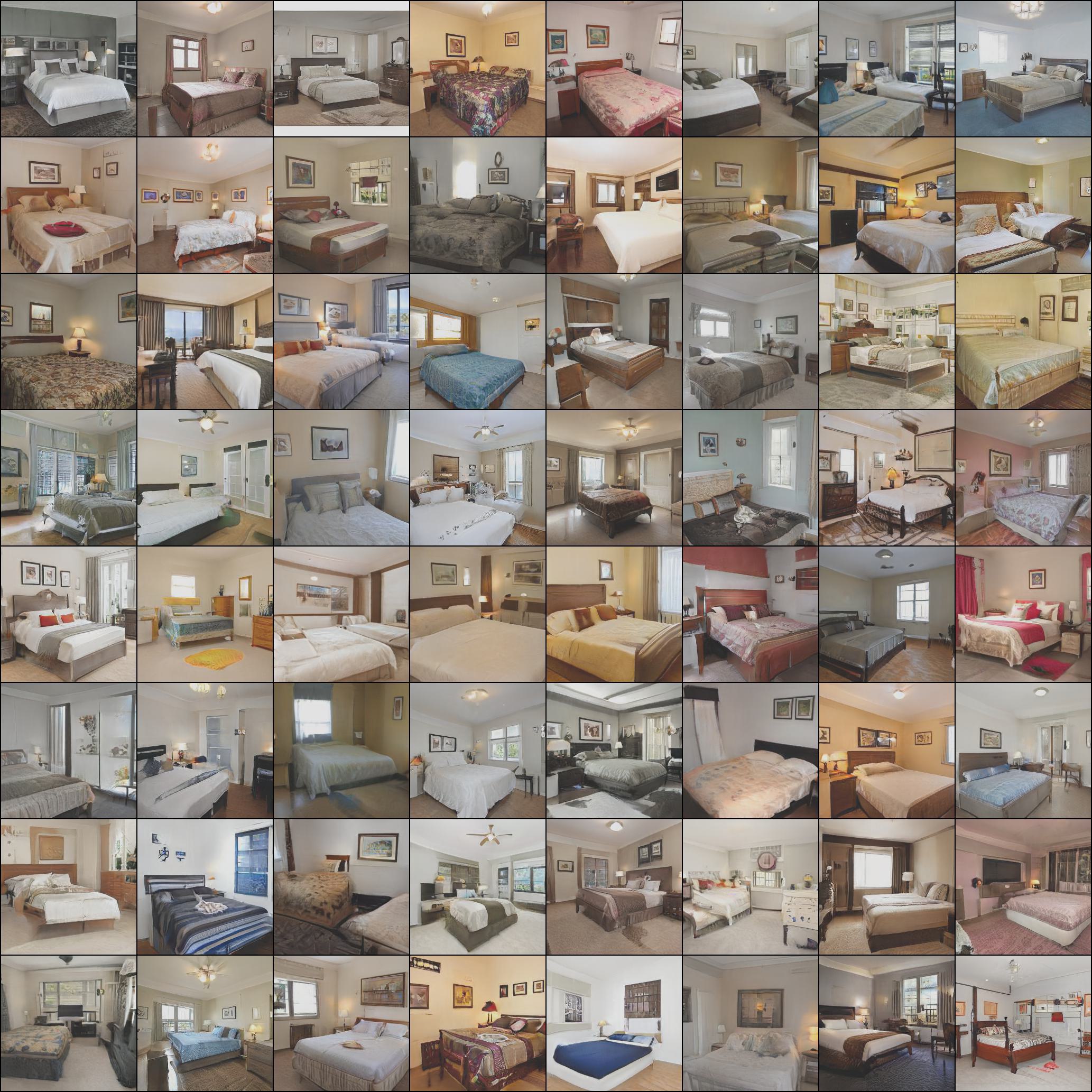
Figure 10: Generated images on bedroom dataset. FID = 4.16. Truncation weight $w=0.3$.

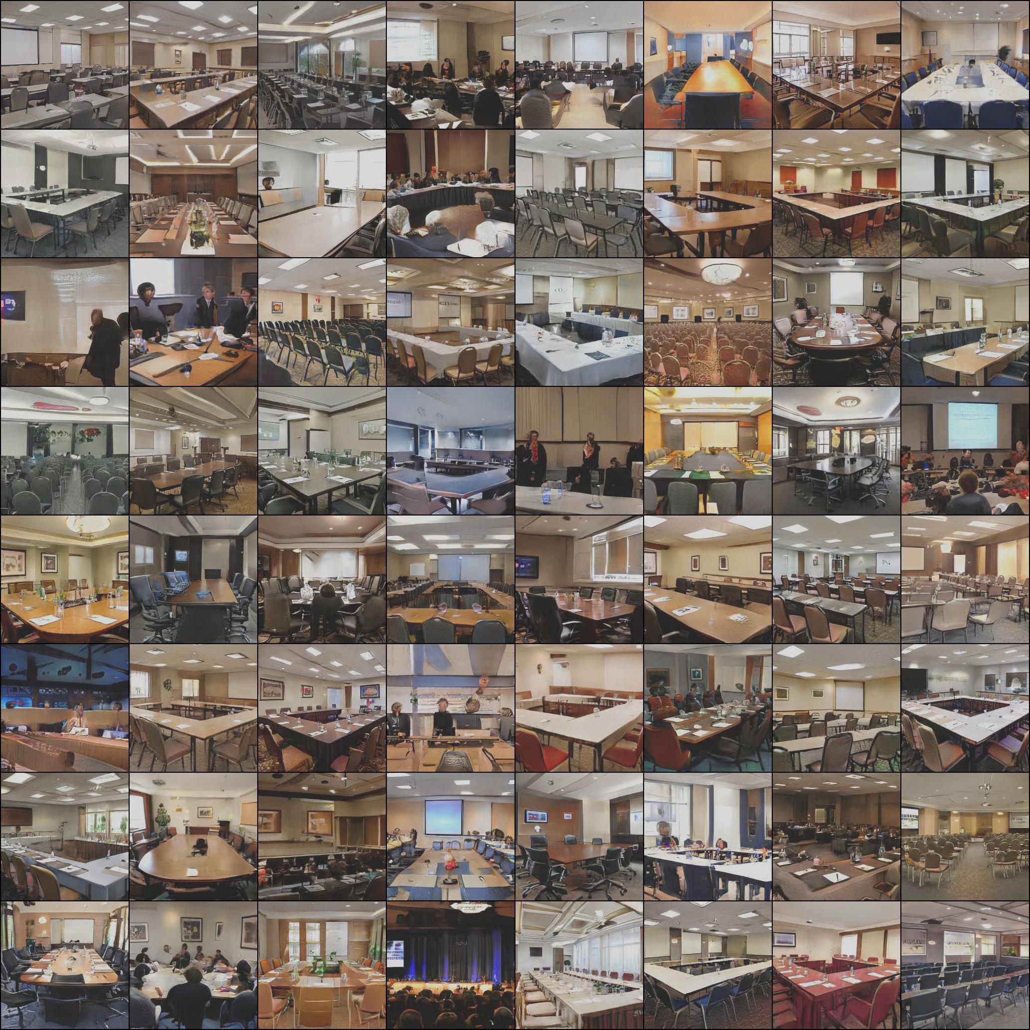
Figure 11: Generated images on conference room dataset. FID = 7.80. Truncation wegiht $w=0.3$.

\begin{overpic}[width=496.85625pt]{figures/editing/moving/bedroom_blob_0.jpg} \put(35.0,30.0){\color[rgb]{1,1,1}\vector(1,0){40.0}} \end{overpic}

\begin{overpic}[width=496.85625pt]{figures/editing/moving/bedroom_blob_2.jpg} \put(55.0,30.0){\color[rgb]{1,1,1}\vector(1,0){40.0}} \end{overpic}

\begin{overpic}[width=496.85625pt]{figures/editing/moving/bedroom_blob_4.jpg} \put(77.0,68.0){\color[rgb]{1,1,1}\vector(1,0){25.0}} \end{overpic}

\begin{overpic}[width=496.85625pt]{figures/editing/moving/bedroom_blob_6.jpg} \put(67.0,72.0){\color[rgb]{1,1,1}\vector(1,0){30.0}} \end{overpic}

\begin{overpic}[width=496.85625pt]{figures/editing/moving/conference_blob_0.jpg} \put(71.0,21.0){\color[rgb]{1,1,1}\vector(1,0){30.0}} \end{overpic}

\begin{overpic}[width=496.85625pt]{figures/editing/moving/conference_blob_2.jpg} \put(58.0,21.0){\color[rgb]{1,1,1}\vector(1,0){30.0}} \end{overpic}

\begin{overpic}[width=496.85625pt]{figures/editing/moving/conference_blob_4.jpg} \put(40.0,58.0){\color[rgb]{1,1,1}\vector(1,0){30.0}} \end{overpic}

\begin{overpic}[width=496.85625pt]{figures/editing/moving/conference_blob_6.jpg} \put(48.0,70.0){\color[rgb]{1,1,1}\vector(1,0){30.0}} \end{overpic}

Figure 12: BlobGAN-3D: Moving an object in the scene. The first row shows the original generated images; the second row shows the corresponding blob layout maps with marks demonstrating the moving direction. The last row shows the synthesized images after moving one blob.

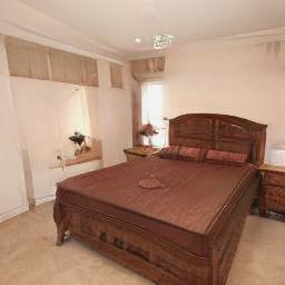
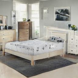
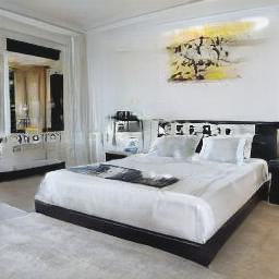
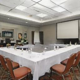
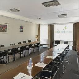
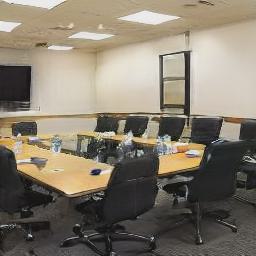
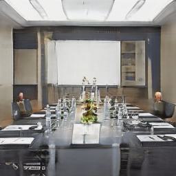
\begin{overpic}[width=496.85625pt]{figures_sup/2d/moving/bedroom_blob_0.jpg} \put(32.0,30.0){\color[rgb]{1,1,1}\vector(1,0){40.0}} \end{overpic}

\begin{overpic}[width=496.85625pt]{figures_sup/2d/moving/bedroom_blob_2.jpg} \put(57.0,27.0){\color[rgb]{1,1,1}\vector(1,0){40.0}} \end{overpic}

\begin{overpic}[width=496.85625pt]{figures_sup/2d/moving/bedroom_blob_4.jpg} \put(80.0,75.0){\color[rgb]{1,1,1}\vector(1,0){25.0}} \end{overpic}

\begin{overpic}[width=496.85625pt]{figures_sup/2d/moving/bedroom_blob_6.jpg} \put(74.0,72.0){\color[rgb]{1,1,1}\vector(1,0){30.0}} \end{overpic}

\begin{overpic}[width=496.85625pt]{figures_sup/2d/moving/conference_blob_0.jpg} \put(51.0,24.0){\color[rgb]{1,1,1}\vector(1,0){30.0}} \end{overpic}

\begin{overpic}[width=496.85625pt]{figures_sup/2d/moving/conference_blob_2.jpg} \put(38.0,21.0){\color[rgb]{1,1,1}\vector(1,0){30.0}} \end{overpic}

\begin{overpic}[width=496.85625pt]{figures_sup/2d/moving/conference_blob_4.jpg} \put(65.0,68.0){\color[rgb]{1,1,1}\vector(1,0){30.0}} \end{overpic}

\begin{overpic}[width=496.85625pt]{figures_sup/2d/moving/conference_blob_6.jpg} \put(60.0,65.0){\color[rgb]{1,1,1}\vector(1,0){30.0}} \end{overpic}

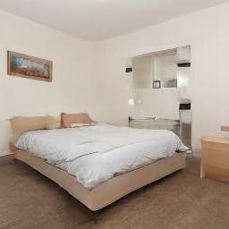
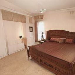
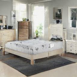
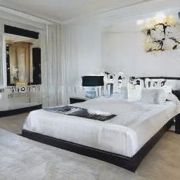
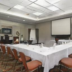
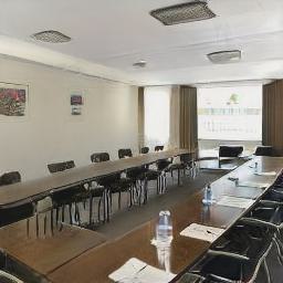
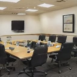
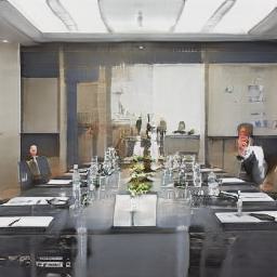
Figure 13: Original BlobGAN: Moving an object in the scene. The first row shows the original generated images; the second row shows the corresponding blob layout maps with marks demonstrating the moving direction. The last row shows the synthesized images after moving one blob. We show these as a comparison to BlobGAN-3D.

\begin{overpic}[width=496.85625pt]{figures/editing/resizing/bedroom_blob_0.jpg} \put(38.0,40.0){\color[rgb]{1,1,1}\line(1,-1){20.0}} \put(58.0,40.0){\color[rgb]{1,1,1}\line(-1,-1){20.0}} \end{overpic}

\begin{overpic}[width=496.85625pt]{figures/editing/resizing/bedroom_blob_2.jpg} \put(43.0,40.0){\color[rgb]{1,1,1}\line(1,-1){20.0}} \put(63.0,40.0){\color[rgb]{1,1,1}\line(-1,-1){20.0}} \end{overpic}

\begin{overpic}[width=496.85625pt]{figures/editing/resizing/bedroom_blob_4.jpg} \put(66.0,70.0){\color[rgb]{1,1,1}\line(1,-1){15.0}} \put(81.0,70.0){\color[rgb]{1,1,1}\line(-1,-1){15.0}} \end{overpic}

\begin{overpic}[width=496.85625pt]{figures/editing/resizing/bedroom_blob_6.jpg} \put(62.0,77.0){\color[rgb]{1,1,1}\line(1,-1){15.0}} \put(77.0,77.0){\color[rgb]{1,1,1}\line(-1,-1){15.0}} \end{overpic}

\begin{overpic}[width=496.85625pt]{figures/editing/resizing/conference_blob_0.jpg} \put(35.0,40.0){\color[rgb]{1,1,1}\line(1,-1){30.0}} \put(63.0,40.0){\color[rgb]{1,1,1}\line(-1,-1){30.0}} \end{overpic}

\begin{overpic}[width=496.85625pt]{figures/editing/resizing/conference_blob_2.jpg} \put(38.0,32.0){\color[rgb]{1,1,1}\line(1,-1){28.0}} \put(64.0,32.0){\color[rgb]{1,1,1}\line(-1,-1){28.0}} \end{overpic}

\begin{overpic}[width=496.85625pt]{figures/editing/resizing/conference_blob_4.jpg} \put(48.0,78.0){\color[rgb]{1,1,1}\line(1,-1){20.0}} \put(68.0,78.0){\color[rgb]{1,1,1}\line(-1,-1){20.0}} \end{overpic}

\begin{overpic}[width=496.85625pt]{figures/editing/resizing/conference_blob_6.jpg} \put(28.0,72.0){\color[rgb]{1,1,1}\line(1,-1){20.0}} \put(48.0,72.0){\color[rgb]{1,1,1}\line(-1,-1){20.0}} \end{overpic}

Figure 14: BlobGAN-3D: Removing an object in the scene. The first row shows the originally generated images; the second row shows the corresponding blob layout maps with marks demonstrating the removed blob. The last row shows the synthesized images after removing one blob.

References

- [1] Rameen Abdal, Peihao Zhu, Niloy J. Mitra, and Peter Wonka. Styleflow: Attribute-conditioned exploration of stylegan-generated images using conditional continuous normalizing flows. ACM Trans. Graph., 40(3), May 2021.
- [2] Titas Anciukevicius, Christoph H. Lampert, and Paul Henderson. Object-centric image generation with factored depths, locations, and appearances, 2020.
- [3] Ivan Anokhin, Kirill Demochkin, Taras Khakhulin, Gleb Sterkin, Victor Lempitsky, and Denis Korzhenkov. Image generators with conditionally-independent pixel synthesis. arXiv preprint arXiv:2011.13775, 2020.
- [4] Mikołaj Bińkowski, Danica J. Sutherland, Michael Arbel, and Arthur Gretton. Demystifying mmd gans, 2018.
- [5] Andrew Brock, Jeff Donahue, and Karen Simonyan. Large scale gan training for high fidelity natural image synthesis, 2018.
- [6] Christopher P. Burgess, Loic Matthey, Nicholas Watters, Rishabh Kabra, Irina Higgins, Matt Botvinick, and Alexander Lerchner. Monet: Unsupervised scene decomposition and representation, 2019.
- [7] Rohan Chabra, Jan Eric Lenssen, Eddy Ilg, Tanner Schmidt, Julian Straub, Steven Lovegrove, and Richard Newcombe. Deep local shapes: Learning local sdf priors for detailed 3d reconstruction, 2020.
- [8] Eric Chan, Marco Monteiro, Petr Kellnhofer, Jiajun Wu, and Gordon Wetzstein. pi-gan: Periodic implicit generative adversarial networks for 3d-aware image synthesis. In Proc. CVPR, 2021.
- [9] Eric R. Chan, Connor Z. Lin, Matthew A. Chan, Koki Nagano, Boxiao Pan, Shalini De Mello, Orazio Gallo, Leonidas Guibas, Jonathan Tremblay, Sameh Khamis, Tero Karras, and Gordon Wetzstein. Efficient geometry-aware 3D generative adversarial networks. In CVPR, 2022.
- [10] Zhiqin Chen and Hao Zhang. Learning implicit fields for generative shape modeling. Proceedings of IEEE Conference on Computer Vision and Pattern Recognition (CVPR), 2019.
- [11] Yunjey Choi, Youngjung Uh, Jaejun Yoo, and Jung-Woo Ha. Stargan v2: Diverse image synthesis for multiple domains, 2019.
- [12] Yu Deng, Jiaolong Yang, Jianfeng Xiang, and Xin Tong. Gram: Generative radiance manifolds for 3d-aware image generation. In Proceedings of the IEEE/CVF Conference on Computer Vision and Pattern Recognition, pages 10673–10683, 2022.
- [13] Martin Engelcke, Adam R. Kosiorek, Oiwi Parker Jones, and Ingmar Posner. Genesis: Generative scene inference and sampling with object-centric latent representations, 2019.
- [14] Dave Epstein, Taesung Park, Richard Zhang, Eli Shechtman, and Alexei A. Efros. Blobgan: Spatially disentangled scene representations, 2022.
- [15] S. M. Ali Eslami, Nicolas Heess, Theophane Weber, Yuval Tassa, David Szepesvari, Koray Kavukcuoglu, and Geoffrey E. Hinton. Attend, infer, repeat: Fast scene understanding with generative models, 2016.
- [16] Kyle Genova, Forrester Cole, Daniel Vlasic, Aaron Sarna, William T. Freeman, and Thomas Funkhouser. Learning shape templates with structured implicit functions, 2019.
- [17] Ian J. Goodfellow, Jean Pouget-Abadie, Mehdi Mirza, Bing Xu, David Warde-Farley, Sherjil Ozair, Aaron Courville, and Yoshua Bengio. Generative adversarial networks, 2014.
- [18] Jiatao Gu, Lingjie Liu, Peng Wang, and Christian Theobalt. Stylenerf: A style-based 3d aware generator for high-resolution image synthesis. In International Conference on Learning Representations, 2022.
- [19] Philipp Henzler, Niloy Mitra, and Tobias Ritschel. Escaping plato’s cave: 3d shape from adversarial rendering, 2018.
- [20] Erik Härkönen, Aaron Hertzmann, Jaakko Lehtinen, and Sylvain Paris. Ganspace: Discovering interpretable gan controls. 2020.
- [21] Justin Johnson, Bharath Hariharan, Laurens van der Maaten, Li Fei-Fei, C. Lawrence Zitnick, and Ross Girshick. Clevr: A diagnostic dataset for compositional language and elementary visual reasoning, 2016.
- [22] Tero Karras, Timo Aila, Samuli Laine, and Jaakko Lehtinen. Progressive growing of gans for improved quality, stability, and variation, 2017.
- [23] Tero Karras, Miika Aittala, Janne Hellsten, Samuli Laine, Jaakko Lehtinen, and Timo Aila. Training generative adversarial networks with limited data. In Proc. NeurIPS, 2020.
- [24] Tero Karras, Miika Aittala, Samuli Laine, Erik Härkönen, Janne Hellsten, Jaakko Lehtinen, and Timo Aila. Alias-free generative adversarial networks, 2021.
- [25] Tero Karras, Samuli Laine, and Timo Aila. A style-based generator architecture for generative adversarial networks, 2018.
- [26] Tero Karras, Samuli Laine, Miika Aittala, Janne Hellsten, Jaakko Lehtinen, and Timo Aila. Analyzing and improving the image quality of stylegan, 2019.
- [27] Adam R. Kosiorek, Hyunjik Kim, Ingmar Posner, and Yee Whye Teh. Sequential attend, infer, repeat: Generative modelling of moving objects, 2018.
- [28] Nupur Kumari, Richard Zhang, Eli Shechtman, and Jun-Yan Zhu. Ensembling off-the-shelf models for gan training, 2021.
- [29] Thomas Leimkühler and George Drettakis. FreeStyleGAN. ACM Transactions on Graphics, 40(6):1–15, dec 2021.
- [30] Yiyi Liao, Katja Schwarz, Lars Mescheder, and Andreas Geiger. Towards unsupervised learning of generative models for 3d controllable image synthesis. In Proceedings of the IEEE/CVF conference on computer vision and pattern recognition, pages 5871–5880, 2020.
- [31] Ilya Loshchilov and Frank Hutter. Decoupled weight decay regularization, 2017.
- [32] Lars Mescheder, Michael Oechsle, Michael Niemeyer, Sebastian Nowozin, and Andreas Geiger. Occupancy networks: Learning 3d reconstruction in function space. In Proceedings IEEE Conf. on Computer Vision and Pattern Recognition (CVPR), 2019.
- [33] Ben Mildenhall, Pratul P. Srinivasan, Matthew Tancik, Jonathan T. Barron, Ravi Ramamoorthi, and Ren Ng. Nerf: Representing scenes as neural radiance fields for view synthesis. In ECCV, 2020.
- [34] Thu Nguyen-Phuoc, Chuan Li, Lucas Theis, Christian Richardt, and Yong-Liang Yang. Hologan: Unsupervised learning of 3d representations from natural images, 2019.
- [35] Thu Nguyen-Phuoc, Christian Richardt, Long Mai, Yong-Liang Yang, and Niloy Mitra. Blockgan: Learning 3d object-aware scene representations from unlabelled images, 2020.
- [36] Michael Niemeyer and Andreas Geiger. Giraffe: Representing scenes as compositional generative neural feature fields. In Proc. IEEE Conf. on Computer Vision and Pattern Recognition (CVPR), 2021.
- [37] Roy Or-El, Xuan Luo, Mengyi Shan, Eli Shechtman, Jeong Joon Park, and Ira Kemelmacher-Shlizerman. Stylesdf: High-resolution 3d-consistent image and geometry generation. In Proceedings of the IEEE/CVF Conference on Computer Vision and Pattern Recognition, pages 13503–13513, 2022.
- [38] Xingang Pan, Xudong Xu, Chen Change Loy, Christian Theobalt, and Bo Dai. A shading-guided generative implicit model for shape-accurate 3d-aware image synthesis. Advances in Neural Information Processing Systems, 34:20002–20013, 2021.
- [39] Eunbyung Park, Jimei Yang, Ersin Yumer, Duygu Ceylan, and Alexander C. Berg. Transformation-grounded image generation network for novel 3d view synthesis, 2017.
- [40] Jeong Joon Park, Peter Florence, Julian Straub, Richard Newcombe, and Steven Lovegrove. Deepsdf: Learning continuous signed distance functions for shape representation. In The IEEE Conference on Computer Vision and Pattern Recognition (CVPR), June 2019.
- [41] Gaurav Parmar, Richard Zhang, and Jun-Yan Zhu. On aliased resizing and surprising subtleties in gan evaluation, 2021.
- [42] Songyou Peng, Michael Niemeyer, Lars Mescheder, Marc Pollefeys, and Andreas Geiger. Convolutional occupancy networks. In European Conference on Computer Vision, pages 523–540. Springer, 2020.
- [43] Thomas Porter and Tom Duff. Compositing digital images. SIGGRAPH Comput. Graph., 18(3):253–259, jan 1984.
- [44] René Ranftl, Katrin Lasinger, David Hafner, Konrad Schindler, and Vladlen Koltun. Towards robust monocular depth estimation: Mixing datasets for zero-shot cross-dataset transfer, 2019.
- [45] Axel Sauer, Kashyap Chitta, Jens Müller, and Andreas Geiger. Projected gans converge faster. In Advances in Neural Information Processing Systems (NeurIPS), 2021.
- [46] Axel Sauer, Katja Schwarz, and Andreas Geiger. Stylegan-xl: Scaling stylegan to large diverse datasets. volume abs/2201.00273, 2022.
- [47] Katja Schwarz, Yiyi Liao, Michael Niemeyer, and Andreas Geiger. Graf: Generative radiance fields for 3d-aware image synthesis. In Advances in Neural Information Processing Systems (NeurIPS), 2020.
- [48] Katja Schwarz, Axel Sauer, Michael Niemeyer, Yiyi Liao, and Andreas Geiger. Voxgraf: Fast 3d-aware image synthesis with sparse voxel grids. arXiv preprint arXiv:2206.07695, 2022.
- [49] Tamar Rott Shaham, Tali Dekel, and Tomer Michaeli. Singan: Learning a generative model from a single natural image, 2019.
- [50] Wenzhe Shi, Jose Caballero, Ferenc Huszár, Johannes Totz, Andrew P. Aitken, Rob Bishop, Daniel Rueckert, and Zehan Wang. Real-time single image and video super-resolution using an efficient sub-pixel convolutional neural network, 2016.
- [51] Zifan Shi, Yujun Shen, Jiapeng Zhu, Dit-Yan Yeung, and Qifeng Chen. 3d-aware indoor scene synthesis with depth priors. 2022.
- [52] Ivan Skorokhodov, Sergey Tulyakov, Yiqun Wang, and Peter Wonka. Epigraf: Rethinking training of 3d gans. arXiv preprint arXiv:2206.10535, 2022.
- [53] Jingxiang Sun, Xuan Wang, Yichun Shi, Lizhen Wang, Jue Wang, and Yebin Liu. Ide-3d: Interactive disentangled editing for high-resolution 3d-aware portrait synthesis, 2022.
- [54] Jingxiang Sun, Xuan Wang, Yong Zhang, Xiaoyu Li, Qi Zhang, Yebin Liu, and Jue Wang. Fenerf: Face editing in neural radiance fields. In Proceedings of the IEEE/CVF Conference on Computer Vision and Pattern Recognition (CVPR), pages 7672–7682, June 2022.
- [55] Shao-Hua Sun. Multi-digit mnist for few-shot learning, 2019.
- [56] Ayush Tewari, Mohamed Elgharib, Gaurav Bharaj, Florian Bernard, Hans-Peter Seidel, Patrick Pérez, Michael Zöllhofer, and Christian Theobalt. Stylerig: Rigging stylegan for 3d control over portrait images, cvpr 2020. In IEEE Conference on Computer Vision and Pattern Recognition (CVPR). IEEE, june 2020.
- [57] Sjoerd van Steenkiste, Karol Kurach, Jürgen Schmidhuber, and Sylvain Gelly. Investigating object compositionality in generative adversarial networks. Neural Networks, 130:309–325, oct 2020.
- [58] Delio Vicini, Sébastien Speierer, and Wenzel Jakob. Differentiable signed distance function rendering. Transactions on Graphics (Proceedings of SIGGRAPH), 41(4):125:1–125:18, July 2022.
- [59] Xudong Xu, Xingang Pan, Dahua Lin, and Bo Dai. Generative occupancy fields for 3d surface-aware image synthesis. Advances in Neural Information Processing Systems, 34:20683–20695, 2021.
- [60] Yinghao Xu, Sida Peng, Ceyuan Yang, Yujun Shen, and Bolei Zhou. 3d-aware image synthesis via learning structural and textural representations. In CVPR, 2022.
- [61] Yang Xue, Yuheng Li, Krishna Kumar Singh, and Yong Jae Lee. Giraffe hd: A high-resolution 3d-aware generative model, 2022.
- [62] Yanchao Yang, Yutong Chen, and Stefano Soatto. Learning to manipulate individual objects in an image, 2020.
- [63] Yasin Yazıcı, Chuan-Sheng Foo, Stefan Winkler, Kim-Hui Yap, Georgios Piliouras, and Vijay Chandrasekhar. The unusual effectiveness of averaging in gan training, 2018.
- [64] Fisher Yu, Ari Seff, Yinda Zhang, Shuran Song, Thomas Funkhouser, and Jianxiong Xiao. Lsun: Construction of a large-scale image dataset using deep learning with humans in the loop, 2015.
- [65] Bowen Zhang, Shuyang Gu, Bo Zhang, Jianmin Bao, Dong Chen, Fang Wen, Yong Wang, and Baining Guo. Styleswin: Transformer-based gan for high-resolution image generation, 2021.
- [66] Han Zhang, Ian Goodfellow, Dimitris Metaxas, and Augustus Odena. Self-attention generative adversarial networks, 2018.
- [67] Kai Zhang, Gernot Riegler, Noah Snavely, and Vladlen Koltun. Nerf++: Analyzing and improving neural radiance fields. arXiv:2010.07492, 2020.
- [68] Xuanmeng Zhang, Zhedong Zheng, Daiheng Gao, Bang Zhang, Pan Pan, and Yi Yang. Multi-view consistent generative adversarial networks for 3d-aware image synthesis. In Proceedings of the IEEE/CVF Conference on Computer Vision and Pattern Recognition, 2022.
- [69] Peng Zhou, Lingxi Xie, Bingbing Ni, and Qi Tian. Cips-3d: A 3d-aware generator of gans based on conditionally-independent pixel synthesis, 2021.
- [70] Jun-Yan Zhu, Taesung Park, Phillip Isola, and Alexei A Efros. Unpaired image-to-image translation using cycle-consistent adversarial networkss. In Computer Vision (ICCV), 2017 IEEE International Conference on, 2017.
- [71] Jun-Yan Zhu, Zhoutong Zhang, Chengkai Zhang, Jiajun Wu, Antonio Torralba, Joshua B. Tenenbaum, and William T. Freeman. Visual object networks: Image generation with disentangled 3d representation, 2018.