Girsanov reweighting for simulations of underdamped Langevin dynamics. Theory.

Abstract

The critical step in a molecular process is often a rare-event and has to be simulated by an enhanced sampling protocol. Recovering accurate dynamical estimates from such biased simulation is challenging. Girsanov reweighting is a method to reweight dynamic properties formulated as path expected values. The path probability is calculated at the time-step resolution of the molecular-dynamics integrator. But the theory is largely limited to overdamped Langevin dynamics. For underdamped Langevin dynamics, the absolute continuity of the path probability ratio for the biased and unbiased potential is not guaranteed, but it depends on the Langevin integrator. We develop a general approach to derive the path probability ratio for Langevin integrators and to analyze whether absolute continuity is fulfilled. We demonstrate our approach on symmetric splitting methods for underdamped Langevin dynamics. For methods that obey absolute continuity, and thus can be used for Girsanov reweighting, we provide an expression for the relative path probability.

I Introduction

Understanding rare events in molecular systems on an atomistic resolution would have great impact in many areas, such as the binding of drug molecules to receptors, protein-protein interactions in molecular machines, aggregation processes in biomolecular systems or artificial materials, phase transitions and chemical reactions. In principle, these processes can be studied by molecular dynamics (MD) simulations [1, 2, 3]. However, the timescale of molecular rare events are often well beyond the timescales that can be reached by direct MD simulations. Even if occasional rare-event transitions can be observed in the course of a direct MD simulation, the estimates of thermodynamic or kinetic properties are often not statistically meaningful. This is because passage times across a barrier into a target state are long-tailed distributed, and the tail contributes to the rare-event estimate. Furthermore, the dynamics in the fast degrees of freedom influence the free-energy surface and the diffusion constant of the rare-event transition in ways that are hard to predict, and any rare event can consist of multiple separate transition paths with different intermediate states and transition states. In short: it is important to sample the full path ensemble that contributes to a rare-event.

One approach to speed up the sampling of rare events is to add a bias to the molecular interaction potential. Enhanced sampling methods like metadynamics[4, 5, 6, 7, 8] and umbrella sampling[9, 10] add energy to the system in order to steer the simulation away from states which have already sufficiently been explored. Since enhanced sampling changes the dynamics of the system, estimates of thermodynamics and dynamic properties are distorted and need to be unbiased. For thermodynamic properties, estimators that accurately reweight the enhanced sampling simulations, such as weighted histogram analysis method [11, 12], are available. With these reweighting techniques, the statistical certainty of thermodynamic properties is drastically increased compared to direct simulations. As a result, the field is moving from direct simulations to combining enhanced sampling with thermodynamic reweighting techniques.

For dynamic properties, on the other hand, one cannot yet routinely use enhanced sampling simulations. In fact, dynamic reweighting techniques are currently a very active field of research [13]. Dynamic properties are path expected values weighted by the path probability density which depends on the potential energy function. Suppose, the system has been simulated at a potential $V$, and one would like to know a dynamic property at a target potential $\widetilde{V}=V+U$. To reweight the corresponding path expected value, one needs the relative path probability, i.e the ratio of the path probabilities at $\widetilde{V}$ and at $V$. Furthermore, the relative path probability needs to obey absolute continuity, i.e. any path that is possible the target potential $\widetilde{V}$ also needs to be possible at the simulation potential $V$.

Several methods to reweight simulations with bias potentials have been proposed in recent years. Usually an effective model of the dynamics is assumed, either a two-state dynamics in which transition state theory or Kramers’ rate theory holds [14, 15, 16, 17, 18] or a Markov state model on a discretized state space[19, 20, 21, 22, 23, 24]. Since the validity of these effective models changes with the potential energy function, they cannot be equally valid at $V$ and at $\widetilde{V}$. It is difficult to judge how this affects the accuracy of the reweighted estimate. We argue that a more accurate approach is to consider the calculation of the path probability ratio as part of the enhanced sampling simulation. In the subsequent analysis, one would use the simulated paths along with the time-series of the relative path probability to reweight the desired dynamic property. For this the relative path probability ratio needs to be calculated at the time-step resolution of the MD simulation, and the corresponding equations need to match the MD integrator. Additionally, at this high time-resolution, the question of absolute continuity needs to be addressed.

Based on works by L. Onsager and S. Machlup [25] and, independently, by I.V. Girsanov [26], one can derive an exact reweighting technique, in which the path probability ratio is calculated at the time-step resolution of the MD simulation. For overdamped Langevin dynamics, the Girsanov theorem guarantees that the relative path probability does not violate absolute continuity, as long as the biasing forces do not approach infinity. This guarantee holds even for continuous solutions of the stochastic differential equation [26, 27]. Additionally, the expression for the relative path probability for time-discretized paths generated by the Euler-Maruyama algorithm is well established [28, 27]. Since the late 1990s, it has been shown several times that Girsanov reweighting or, equivalently, dynamic importance sampling can be used to unbias overdamped Langevin dynamics, both for model potentials [29, 30, 31, 32, 33] and for small molecular systems [34, 35, 36]. But the use of overdamped Langevin dynamics to model molecular rare events is limited. It can be used in the mesoscopic molecular regime, in which molecules are (partly) treated as rigid bodies, to study molecular crowding effects, association processes between large molecules, and even the dynamics of coarse-grained polymers [37, 38] But because overdamped Langevin dynamics suppresses the fast intramolecular fluctuations, it cannot be used to model conformational transitions at atomistic resolutions.

By contrast, underdamped Langevin dynamics, often under the name ,,Langevin thermostats”, is an accurate and frequently used equation of motion for atomistic MD [39]. For continuous solutions of underdamped Langevin dynamics, the path probability can be formulated[40], but one cannot guarantee that the relative path probability obeys absolute continuity. This, at first, seems like an impasse in the attempt to unbias dynamic estimates: one needs to sample the molecular rare events by underdamped Langevin dynamics, but for underdamped Langevin dynamics the relative path probability might not exist. Fortunately, when reweighting a MD simulation, the path expected value is not calculated for time-continuous paths but for time-discretized paths. As explained above, an accurate reweighting method needs to calculate the relative path probability at the time resolution at which the path is produced. Thus, depending on the integrator used to propagate the underdamped Langevin dynamics, the relative path probability density may exist after all, and Girsanov reweighting may become possible. Our approach is therefore not to discretize the continuous path integral. [33]. Instead we start from already existing algorithms to propagate the equation of motion for underdamped Langevin dynamics and derive the relative path probability for the resulting time-discretized paths.

Girsanov reweighting for underdamped Langevin dynamics has first been reported in Refs. 41 and 42. In Ref. 43 we introduced a formulation of the path probability ratio as a function of the random numbers generated during the simulation potential at $V$ and a random number difference to $\widetilde{V}$, which we called reweighting on-the-fly. This allowed us on the one hand to efficiently calculate part of the relative path probability already during the simulation. On the under hand, it allowed us to approximate the relative path probability for underdamped Langevin dynamics. With this approximation, we could reweight metadynamics simulations of the folding equilibrium of $\beta$-hairpin peptide [44]. In Ref. 45 we analyzed this approximation and derived the path probability ratio for a simple Langevin integrator.

The goal of this contribution is to develop a general approach to derive the path probability for Langevin integrators and to analyze whether the relative path probability obeys absolute continuity. We focus on symmetric splitting methods for underdamped Langevin dynamics [46, 47, 48, 49], and additionally include a closely related[50] variant[51, 52] which is used as default Langevin thermostat in several MD simulation programs [53, 54, 55]. For methods that obey absolute continuity, and thus can be used for Girsanov reweighting, we provide an expression for the relative path probability.

We chose symmetric splitting methods, because their derivation is documented in great detail [46, 47, 48, 49, 56], which provides an easy entry point for our analysis. Additionally, the convergence properties of this class of integrators are well-understood [48, 57, 58, 59]. However, the development of integrators for underdamped Langevin dynamics has been a very active field for decades and many other algorithms have been proposed [60, 61, 62, 63, 64, 65, 66, 67, 68, 69, 70, 71, 72, 73, 74, 75]. We believe our approach to derive the path probability ratio can be applied to these Langevin integrators, too.

The article is structured as follows: In sections II and III we review the theory of Girsanov reweighting and of symmetric splitting algorithms. Sections IV and V contain our analysis of these integrators and the derivation of the relative path probabilities. In section VI we introduce a graphical representation of Langevin integrators that helped us to visualize and classify the effects of changeing the potential energy on the behaviour of the Langevin integrator. Section VII contains a short discussion and outlook.

II Girsanov reweighting

II.1 Equation of motion, path probability density, and path integral

Consider a particle with mass $m$ that moves in a one-dimensional position space $q\in\mathbb{R}$ according to underdamped Langevin dynamics

$$\dot{q} =\frac{p}{m}$$ (1)

$$\dot{p} =-\nabla_{q}V(q)-\xi p+\sqrt{2\xi k_{B}Tm}\,\eta(t)\,,$$ (2)

In eq. 2, $V(q)$ is the potential energy function, $\nabla_{q}=\partial/\partial q$ denotes the gradient with respect to the position coordinate, $\xi$ is a collision or friction rate (in units of s^-1), $T$ is the temperature and $k_{B}$ is the Boltzmann constant. $\eta\in\mathbb{R}$ is an uncorrelated Gaussian white noise with unit variance centered at zero $\langle\eta(t)\eta(t^{\prime})\rangle=\delta(t-t^{\prime})$, where $\delta(t-t^{\prime})$ is the Dirac delta-function. We use the dot-notation for derivatives with respect to time: $\dot{q}=\partial q/\partial t$. $x(t)=(q(t),p(t))\in\Gamma\subset\mathbb{R}^{2}$ denotes the state of the system at time $t$, which consists of positions $q(t)$ and conjugated momenta $p(t)=m\dot{q}(t)$. $\Gamma$ is called state space or phase space of the system.

A Langevin integrator yields a time-discretised solution of eq. 2: $\mathbf{x}=(x_{0},x_{1},x_{2},\dots x_{n})$. The path $\mathbf{x}$ is a sequence of $n+1$ states $x_{k}=(q_{k},p_{k})\in\Gamma$, where consecutive states $x_{k}$ and $x_{k+1}$ are separated by a (small) time step $\Delta t$, $q_{k}$ is the position at time $k\Delta t$, and $p_{k}$ is the momentum at time $k\Delta t$. $x_{0}=(q_{0},p_{0})$ is the initial state of the path, and $\tau=n\Delta t$ is the path length.

A time-discretized path $\mathbf{x}$ is an element of the space $\mathcal{S}=\Gamma^{n+1}$. Its path probability density is $\mathcal{P}[\mathbf{x}]=p(x_{0})\cdot\mathcal{P}[x_{1}\dots x_{n}|x_{0}]\,,$ where we wrote the path probability as a product of the probability density of the intial state $p(x_{0})$ and the conditional probability of the path $\mathcal{P}[x_{1}\dots x_{n}|x_{0}]$, given that the path starts in $x_{0}$. The Langevin integrators considered in this contribution implement a Markov process. That is, the probability to observe the state $x_{k+1}$ at time $t=(k+1)\Delta t$ depends only on the previous state $x_{k}$ at time $t=k\Delta t$ and not on any of the states before that, i.e. $p(x_{k+1}|x_{k},x_{k-1}\dots x_{0})=p(x_{k+1}|x_{k})$. The path probability density to observe a particular path $\mathbf{x}$ can then be written as a product of the single-step transition probabilities $p(x_{k+1}|x_{k})$

$$P[\mathbf{x}]=p(x_{0})\cdot P[x_{1}\dots x_{n}|x_{0}] = p(x_{0})\cdot\prod_{k=0}^{n-1}p(x_{k+1}|x_{k})\,.$$ (3)

The probability density of the initial state depends on the setup of the computational experiment. Here, we assume that the path $\mathbf{x}$ is a short snippet of a long equilibrium trajectory. Then we can assume that $p(x_{0})$ is distributed according to the Boltzmann distribution

$$p(x_{0}) = p(q_{0},p_{0})=\frac{1}{Z}\exp\left(-\frac{V(q_{0})}{k_{B}T}\right)\cdot\frac{1}{\sqrt{2\pi k_{B}Tm}}\exp\left(-\frac{1}{k_{B}T}\frac{p_{0}^{2}}{2m}\right)\,,$$ (4)

where $Z=\int_{-\infty}^{\infty}\mathrm{d}q_{0}\,\exp\left(-\frac{V(q_{0})}{k_{B}T}\right)$ is the classical partition function. The functional form of the single-step transition probability depends on the Langevin integrator, and it is the aim of this contribution to analyze $p(x_{k+1}|x_{k})$ for various integrators.

The path probability density $P[\mathbf{x}]$ is normalised as

$$\int_{\mathcal{S}}\mathcal{D}\mathbf{x}\,\mathcal{P}[\mathbf{x}]=\int_{x_{0}\in\Gamma}\int_{x_{1}\in\Gamma}\dots\int_{x_{n}\in\Gamma}\mathrm{d}x_{0}\mathrm{d}x_{1}\dots\mathrm{d}x_{n}\;\mathcal{P}[\mathbf{x}] = 1\,,$$ (5)

where the first equality defines the path integral $\int_{\mathcal{S}}\mathcal{D}\mathbf{x}\dots$.

Let $s:\mathcal{S}\rightarrow\mathbb{R}$ be a path observable, i.e. a function that maps a time-discretised path to a number. The path expected value of this observable is

$$\langle s\rangle=\int\mathcal{D}\mathbf{x}\,\mathcal{P}[\mathbf{x}]s[\mathbf{x}]=\int_{x_{0}\in\Gamma}\int_{x_{1}\in\Gamma}\dots\int_{x_{n}\in\Gamma}\mathrm{d}x_{0}\mathrm{d}x_{1}\dots\mathrm{d}x_{n}\;\mathcal{P}[\mathbf{x}]s[\mathbf{x}]\,,$$ (6)

Assuming ergodicity, this path expected value can be estimated from a set of $N$ paths $(\mathbf{x}_{1},\mathbf{x}_{2}\dots\mathbf{x}_{N})$ that has been sampled according to $\mathcal{P}[\mathbf{x}]$

$$\langle s\rangle = \lim_{N\rightarrow\infty}\frac{1}{N}\,\sum_{i=1}^{N}s[\mathbf{x}_{i}]\,.$$ (7)

A short comment on notation: we denote functions of paths $\mathbf{x}$ with square brackets around the argument, and functions of states $x=(q,p)$ with round brackets.

II.2 Girsanov reweighting

In Girsanov reweighting, one samples paths at a simulation potential $V(q)$, and from this sample one estimates path expected values at a target potential

$$\widetilde{V}(q) = V(q)+U(q)\,,$$ (8)

where $U(q)$ is called bias or perturbation potential. Let us point out the sign convention. In eq. 8, we add the perturbation $U$ to the simulation potential $V$, which is the convention used in the literature on path reweighting. The literature on enhanced sampling simulations uses the opposite sign convention, i.e. the bias is subtracted from the simulation potential to obtain to the true (target) potential: $\widetilde{V}=V-U_{\mathrm{enh.}\,\mathrm{samp.}}$. Thus, if Girsanov reweighting is used to unbias enhanced sampling simulations, the bias in eq. 8 is $U=-U_{\mathrm{enh.}\,\mathrm{samp.}}$.

We assume that $\widetilde{V}$ represents a typical molecular potential, i.e. a function that has infinite discontinuities whenever two atoms occupy the same position, but is continuous and differentiable everywhere else. We further assume that $U(q)$ respects these discontinuities and does not introduce any new discontinuities. In practice this means that one cannot use soft-core potentials [76, 77] to construct $U(q)$.

Formally, one can reweight the path expected value at the target potential as

$$\widetilde{\langle s\rangle}=\int\mathcal{D}\mathbf{x}\,\widetilde{\mathcal{P}}[\mathbf{x}]s[\mathbf{x}]=\int\mathcal{D}\mathbf{x}\,g(x_{0})M[\mathbf{x}|x_{0}]\,\mathcal{P}[\mathbf{x}]s[\mathbf{x}]\,,$$ (9)

where $\widetilde{\mathcal{P}}[\mathbf{x}]$ is the path probability density at $\widetilde{V}$, and

$$g(x_{0})\cdot M[\mathbf{x}|x_{0}] = \frac{\widetilde{p}(x_{0})}{p(x_{0})}\cdot\frac{\widetilde{\mathcal{P}}[x_{1}\dots x_{n}|x_{0}]}{\mathcal{P}[x_{1}\dots x_{n}|x_{0}]}$$ (10)

is the path reweighting factor. If $\widetilde{p}(x_{0})$ and $p(x_{0})$ are given by eq. 4 (for $\widetilde{V}$ and $V$, respectively), then the relative weight of the initial state is

$$g(x_{0}) = \frac{\widetilde{p}(x_{0})}{p(x_{0})}=\frac{Z}{\widetilde{Z}}\exp\left(-\frac{1}{k_{B}T}U(q_{0})\right)\,.$$ (11)

If $M[\mathbf{x}|x_{0}]$ exists and one can find a computable expression for it, then one can estimate the path expected value at the target potential, $\widetilde{\langle s\rangle}$ from paths sampled at the simulation potential $(\mathbf{x}_{1},\mathbf{x}_{2}\dots\mathbf{x}_{N})$ by reweighting their contribution to the estimator

$$\widetilde{\langle s\rangle} = \lim_{N\rightarrow\infty}\frac{1}{N}\,\sum_{i=1}^{N}g(x_{i,0})M[\mathbf{x}_{i}|x_{i,0}]\cdot s[\mathbf{x}_{i}]\,.$$ (12)

where $g(x_{i,0})M[\mathbf{x}_{i}|x_{i,0}]$ is the relative weight of path $\mathbf{x}_{i}$ a the target potential $\widetilde{V}$. Whether $M[\mathbf{x}|x_{0}]$ exists, depends on the underlying dynamics, specifically on the condition of absolute continuity.

II.3 Absolute continuity

The path probability density $\widetilde{\mathcal{P}}[\mathbf{x}]$ at the target potential and the path probability density $\mathcal{P}[\mathbf{x}]$ at the simulation potential are absolutely continuous with respect to each other [26, 27, 43, 78] if

$$\widetilde{\mathcal{P}}[S]=\int_{S\subset\mathcal{S}}\mathcal{D}\mathbf{\mathbf{x}}\,\widetilde{\mathcal{P}}[\mathbf{x}]=0 \Leftrightarrow \mathcal{P}[S]=\int_{S\subset\mathcal{S}}\mathcal{D}\mathbf{\mathbf{x}}\,\mathcal{P}[\mathbf{x}]=0\,,$$ (13)

where $S=S_{0}\times S_{1}\times\dots\times S_{n}$ is a small subset of the path space $\mathcal{S}$, a and $S_{i}$ is a small region in phase space $\Gamma$ in which $x_{i}$ may be found. That is, any region of the path space $\mathcal{S}$ that is sampled by the dynamics at $\widetilde{V}(x)$ also needs to be sampled by the dynamics at $V(x)$, and vice versa. Otherwise the relative path probability density in eq. 10 is not defined.

(Strictly speaking only $\widetilde{\mathcal{P}}$ needs to be absolutely continuous with respect to $\mathcal{P}$. But since this almost surely implies[27] that also $\mathcal{P}$ is absolutely continuous with respect to $\widetilde{\mathcal{P}}$, we here omit this distinction.)

If $P[\mathbf{x}]$ and $\widetilde{P}[\mathbf{x}]$ can be decomposed as in eq. 3, absolute continuity is fulfilled if

$$\widetilde{p}(S_{0})=\int_{S_{0}}\mathrm{d}x_{0}\,\widetilde{p}(x_{0})\,=0 \Leftrightarrow p(S_{0})=\int_{S_{0}}\mathrm{d}x_{0}\,p(x_{0})\,=0$$ (14)

and if

$$\widetilde{p}(S_{k+1}|x_{k})=\int_{S_{k+1}}\mathrm{d}x_{k+1}\,\widetilde{p}(x_{k+1}|x_{k})\,=0 \Leftrightarrow p(S_{k+1}|x_{k})=\int_{S_{k+1}}\mathrm{d}x_{k+1}\,p(x_{k+1}|x_{k})\,=0\,.$$ (15)

for all $k$ with $k=0,1\dots,n-1$. Eq. 14 is fulfilled if $\widetilde{p}(x_{0})$ and $p(x_{0})$ are given by eq. 4 (for $\widetilde{V}$ and $V$, respectively), but other choices are also possible. For overdamped Langevin dynamics, the Girsanov theorem guarantees that - for sensible choices of $U(q)$ (see section II.2) - eq. 15 is fulfilled. Thus for overdamped Langevin dynamics, $M[\mathbf{x}|x_{0}]$ exists, and for overdamped time-discretized paths generated by the Euler-Maruyama scheme [28, 27], the computable expression for $M[\mathbf{x}|x_{0}]$ is well-established [27, 31, 42, 33, 35, 43, 44]. By contrast, the existence of $M[\mathbf{x}|x_{0}]$ cannot be guaranteed for underdamped Langevin dynamics (eq. 2). It may however exist for time-discretized paths of underdamped Langevin dynamics. In sections IV and V, we will discuss the existence of $M[\mathbf{x}|x_{0}]$ for symmetric splitting schemes [46, 47, 48, 49] for underdamped Langevin dynamics.

II.4 Reweighting on-the-fly

To derive $M[\mathbf{x}|x_{0}]$, we use reweighting on-the-fly (proposed in Ref. 43 and discussed in more detail in Ref. 45). In this approach, the reweighting factor is formulated in terms of the random numbers $\eta_{k}$, which are generated during the simulation at $V$, and a random number difference $\Delta\eta_{k}$, which depends on the gradient of the bias $\nabla U$. Both properties are easily accessible during the simulation, and part of the reweighting factor can be pre-calculated on-the-fly during the simulation. This makes the actual reweighting (eq. 12) computationally simple and efficient.

A stochastic integrator generates a sequence of random numbers $\bm{\eta}=(\eta_{0},\eta_{1},\dots,\eta_{n-1})$ to represent the random force in a stochastic equation of motion (e.g. eq. 2). The random numbers $\eta_{k}$ are usually drawn from a Gaussian normal distribution with zero mean and unit variance

$$P(\eta_{k}) = \sqrt{\frac{1}{2\pi}}\exp\left(-\frac{1}{2}\eta_{k}^{2}\right)\,.$$ (16)

If the initial state $x_{0}$ has been set and $\bm{\eta}$ has been generated, the path $\mathbf{x}|x_{0}=(x_{1}\dots x_{n}|x_{0})$ is fully determined. Thus, the stochastic integrators can be viewed as a map from a random number sequence $\bm{\eta}$ to a path $\mathbf{x}|x_{0}$. If the map is bijective (one-to-one mapping between random number sequence and path), the conditional path probability density is equal to the probability of drawing the corresponding sequence of random numbers:

$$\mathcal{P}[\mathbf{x}|x_{0}] = \mathcal{P}[\bm{\eta}]=\frac{1}{\sqrt[n]{2\pi}}\exp\left(-\frac{1}{2}\sum_{k=0}^{n-1}\eta_{k}^{2}\right)\,.$$ (17)

The stochastic integrator evaluates the gradient of the potential $V$, and therefore the map depends on $V$. If the potential is modified from $V$ to the target potential $\widetilde{V}$, the map changes accordingly, and a different random number sequence $\bm{\widetilde{\eta}}$ is needed to generate the same path $\mathbf{x}|x_{0}$. The conditional path probability density at $\widetilde{V}$ is then equal to the probability of drawing $\bm{\widetilde{\eta}}$: $\widetilde{\mathcal{P}}[\mathbf{x}|x_{0}]=\mathcal{P}[\widetilde{\bm{\eta}}]$.

At each integration step $k$, the random numbers $\eta_{k}$ and $\tilde{\eta}_{k}$ differ by $\Delta\eta_{k}$:

$$\tilde{\eta}_{k} = \eta_{k}+\Delta\eta_{k}\,.$$ (18)

This allows us to write the relative conditional path probability density as [45]

$$M[\mathbf{x}|x_{0}]=\frac{\widetilde{\mathcal{P}}[\mathbf{x}|x_{0}]}{\mathcal{P}[\mathbf{x}|x_{0}]}=\frac{\mathcal{P}[\widetilde{\bm{\eta}}]}{\mathcal{P}[\bm{\eta}]} = \exp\left(-\sum_{k=0}^{n-1}\eta_{k}\cdot\Delta\eta_{k}\right)\cdot\exp\left(-\frac{1}{2}\sum_{k=0}^{n-1}(\Delta\eta_{k})^{2}\right)\,.$$ (19)

The random numbers $\eta_{k}$ are recorded during the simulation at $V$; the expression for $\Delta\eta_{k}$ depends on the stochastic integrator.

The discussion so far applies to stochastic integrators that generate one random number $\eta_{k}$ per integration step and degree of freedom. Some symmetric splitting methods for underdamped Langevin dynamics however generate two random numbers $(\eta_{k}^{(1)},\eta_{k}^{(2)})$ per integration step and degree of freedom. The two random numbers are drawn independently from a Gaussian normal distribution with zero mean and unit variance, i.e. $P(\eta_{k}^{(1)},\eta_{k}^{(2)})=P(\eta_{k}^{(1)})P(\eta_{k}^{(2)})$, and $P(\eta_{k}^{(1)})$ and $P(\eta_{k}^{(2)})$ are given by eq. 16. Thus, an integrator with two random numbers per integration step can be viewed as a map from two sequences of random numbers $(\bm{\eta}^{(1)},\bm{\eta}^{(2)})$ to a path $\mathbf{x}|x_{0}$, where $\bm{\eta}^{(1)}=(\eta_{0}^{(1)},\eta_{1}^{(1)},\dots,\eta_{n-1}^{(1)})$ and $\bm{\eta}^{(2)}=(\eta_{0}^{(2)},\eta_{1}^{(2)},\dots,\eta_{n-1}^{(2)})$. If the map is bijective, the conditional path probability density is equal to the probability of drawing the two random number sequences:

$$\mathcal{P}[\mathbf{x}|x_{0}] = \mathcal{P}[\bm{\eta}^{(1)},\bm{\eta}^{(2)}]=\frac{1}{\sqrt[n]{2\pi}}\exp\left(-\frac{1}{2}\sum_{k=0}^{n-1}\left(\eta_{k}^{(1)}\right)^{2}\right)\cdot\frac{1}{\sqrt[n]{2\pi}}\exp\left(-\frac{1}{2}\sum_{k=0}^{n-1}\left(\eta_{k}^{(2)}\right)^{2}\right)\,.$$ (20)

At the target potential $\widetilde{V}$, two different random number sequences $\widetilde{\bm{\eta}}^{(1)}=(\widetilde{\eta}^{(1)}_{0},\widetilde{\eta}^{(1)}_{1},\dots,\widetilde{\eta}^{(1)}_{n-1})$ and $\widetilde{\bm{\eta}}^{(2)}=(\widetilde{\eta}^{(2)}_{0},\widetilde{\eta}^{(2)}_{1},\dots,\widetilde{\eta}^{(2)}_{n-1})$ are needed to generate the same path $\mathbf{x}$. At each integration step $k$, the random numbers differ by $\Delta\eta^{(1)}_{k}$ and $\Delta\eta^{(2)}_{k}$:

$$\widetilde{\eta}^{(1)}_{k} = \eta^{(1)}_{k}+\Delta\eta^{(1)}_{k}$$ (21)

$$\widetilde{\eta}^{(2)}_{k} = \eta^{(2)}_{k}+\Delta\eta^{(2)}_{k}\,.$$ (22)

The relative conditional path probability density can then be written as

$$M[\mathbf{x}|x_{0}] = \frac{\widetilde{\mathcal{P}}[\mathbf{x}\,|\,x_{0}]}{\mathcal{P}[\mathbf{x}\,|\,x_{0}]}=\frac{P[\widetilde{\bm{\eta}}^{(1)},\widetilde{\bm{\eta}}^{(2)}]}{P[\bm{\eta}^{(1)},\bm{\eta}^{(2)}]}$$ (23)

$$= \exp\left(-\sum\limits_{k=0}^{n-1}\eta^{(1)}_{k}\cdot\Delta\eta^{(1)}_{k}\right)\cdot\exp\left(-\frac{1}{2}\sum\limits_{k=0}^{n-1}(\Delta\eta^{(1)}_{k})^{2}\right)\cdot$$ (25)

$$\exp\left(-\sum\limits_{k=0}^{n-1}\eta^{(2)}_{k}\cdot\Delta\eta^{(2)}_{k}\right)\cdot\exp\left(-\frac{1}{2}\sum\limits_{k=0}^{n-1}(\Delta\eta^{(2)}_{k})^{2}\right)\,.$$

As in eq. 19, the random numbers $\eta_{k}^{(1)}$ and $\eta_{k}^{(2)}$ are recorded during the simulation at $V$, and the expressions for $\Delta\eta_{k}^{(1)}$ and $\Delta\eta_{k}^{(2)}$ depend on the integrator.

At this point the obstacle in constructing path reweighting factors for underdamped Langevin dynamics becomes noticeable. In underdamped Langevin dynamics, the state $x_{k}=(q_{k},p_{k})$ is a two-dimensional vector. Thus, integrators with two random numbers per integration step map two real numbers to a two-dimensional state space, whereas integrators with one random number map a single real number to a two-dimensional state space. In both cases, $P[\mathbf{x}|x_{0}]$ can be derived from the integrator equations (see section III and supplementary material), but $M[\mathbf{x}|x_{0}]$ does not exist for all integrators (see sections IV and V).

III Langevin integrators

III.1 Equation of motion and splitting methods

Eq. 2 can be reformulated as a vector field

$$\left(\begin{array}[]{c}\dot{q}\\ \dot{p}\end{array}\right) =\underbrace{\left(\begin{array}[]{c}p/m\\ 0\end{array}\right)}_{A}+\underbrace{\left(\begin{array}[]{c}0\\ -\nabla_{q}V(q)\end{array}\right)}_{B}+\underbrace{\left(\begin{array}[]{c}0\\ -\xi p+\sqrt{2\xi k_{B}Tm}\,\eta(t)\end{array}\right)}_{O}\,.$$ (34)

Each of the three terms, $A$, $B$ and $O$, can be integrated separately to yield the following time-discretized update operators

$$\mathcal{A}\left(\begin{array}[]{c}q_{k}\\ p_{k}\end{array}\right) =\left(\begin{array}[]{c}q_{k}+\Delta t\frac{1}{m}p_{k}\\ p_{k}\end{array}\right)=\left(\begin{array}[]{c}q_{k}+ap_{k}\\ p_{k}\end{array}\right)$$ (35g)

$$\mathcal{B}\left(\begin{array}[]{c}q_{k}\\ p_{k}\end{array}\right) =\left(\begin{array}[]{c}q_{k}\\ p_{k}-\Delta t\nabla V(q_{k})\end{array}\right)=\left(\begin{array}[]{c}q_{k}\\ p_{k}+b(q_{k})\end{array}\right)$$ (35n)

$$\mathcal{O}\left(\begin{array}[]{c}q_{k}\\ p_{k}\end{array}\right) =\left(\begin{array}[]{c}q_{k}\\ e^{-\xi\Delta t}p_{k}+\sqrt{k_{B}Tm(1-e^{-2\xi\Delta t})}\,\eta_{k}\end{array}\right)=\left(\begin{array}[]{c}q_{k}\\ d\,p_{k}+f\,\eta_{k}\end{array}\right)\,,$$ (35u)

with time step $\Delta t$ and random number $\eta_{k}\sim\mathcal{N}(0,1)$, where $\mathcal{N}(\mu,\sigma^{2})$ denotes the Gaussian normal distribution with mean $\mu$ and variance $\sigma^{2}$. Eqs. 35g – 35u are the time-discretized solutions of their respective parts in the differential equation (eq. 34), where 35u is the result known from the Ornstein-Uhlenbeck process (see Chapter 7.3.1. in Ref. 56). The second equality introduces the following abbreviations to keep the notation manageable

$$a = \Delta t\frac{1}{m}$$ (36a)

$$b(q_{k}) = -\Delta t\nabla V(q_{k})$$ (36b)

$$d = e^{-\xi\Delta t}$$ (36c)

$$f = \sqrt{k_{B}Tm(1-e^{-2\xi\Delta t})}$$ (36d)

where $d$ stands for dissipation and $f$ for the thermal fluctuation.

Particularly accurate Langevin integration schemes can be derived using the (symmetric) operator splitting method, or Strang splitting [79, 70]. In these algorithms, some of the update operators (eqs. 35g, 35n, and 35u) are carried out twice during an integration step, but each time with only half a time step $\frac{\Delta t}{2}$. If a step is carried out for only half a time step $\frac{\Delta t}{2}$, we denote the corresponding operator with a prime, e.g.

$$\mathcal{A^{\prime}}\left(\begin{array}[]{c}q_{k}\\ p_{k}\end{array}\right) =\left(\begin{array}[]{c}q_{k}+\frac{\Delta t}{2}\frac{1}{m}p_{k}\\ p_{k}\end{array}\right)=\left(\begin{array}[]{c}q_{k}+a^{\prime}p_{k}\\ p_{k}\end{array}\right)\,.$$ (43)

Correspondingly, $a^{\prime}$, $b^{\prime}$, $d^{\prime}$ and $f^{\prime}$ are obtained by replacing $\Delta t$ with $\Delta t/2$ in eqs. 149a-149d. For an in-depth discussion on the theory of splitting operators we refer to Refs. 79, 80, 70, 47, 48 and Chapter 7 in Ref. 81.

In this contribution, we will use the ABO method to illustrate our approach, and we will apply the approach to the following integrators based on eq. 34: ABOBA, BAOAB, OABAO, AOBOA, OBABO (Bussi-Parrinello thermostat), and BOAOB [46, 47, 48, 49, 58]. These algorithsm are implemented in OpenMM [53] via the package OpenMMTools [59]. We additionally include BAOA [51], because it is implemented in several MD simulations packages [53, 54, 55], where it is sometimes called Verlet-Middle integrator [73]. GROMACS implements the GROMACS stochastic dynamics (GSD) method [52], which is equivalent to BAOA [50].

III.2 Example: ABO method

The Langevin integrator that is constructed by carrying out eqs. 35g, 35n and 35u consecutively is called ABO method (sequential splitting [79, 70]). The ABO algorithm yields a less accurate approximation to the actual dynamics than symmetric splitting methods (or equivalently: a small time step $\Delta t$ is needed to obtain a given accuracy). Here, we use it to illustrate concepts.

The integrator equations of the ABO algorithm are

$$q_{k+1} =q_{k}+ap_{k}$$ (44a)

$$p_{k+1/2} =p_{k}+b(q_{k+1})$$ (44b)

$$p_{k+1} =dp_{k+1/2}+f\eta_{k}\,.$$ (44c)

$p_{k+1/2}$ should not be interpreted as an integration by half a time step, but rather as 50% progress in the update of the momenta. Namely, in eq. 44b the momentum is updated according to the forces due to the potential energy function, and in eq. 44c the momentum update due to friction and random forces is carried out. The contributions of these two steps to the total momentum update are by no means equal.

The joint update of the position and momentum, i.e. the update operator of the ABO method $\mathcal{U}_{\mathrm{ABO}}$, is obtained by sequentially applying operators $\mathcal{A}$, $\mathcal{B}$, and $\mathcal{O}$ to the current state $(q_{k},p_{k})^{\top}$.

$$\left(\begin{array}[]{c}q_{k+1}\\ p_{k+1}\end{array}\right) = \mathcal{U}_{\mathrm{ABO}}\left(\begin{array}[]{l}q_{k}\\ p_{k}\end{array}\right)$$ (49)

$$= \mathcal{O}\mathcal{B}\mathcal{A}\left(\begin{array}[]{l}q_{k}\\ p_{k}\end{array}\right)$$ (52)

$$= \mathcal{O}\mathcal{B}\left(\begin{array}[]{l}q_{k}+ap_{k}\\ p_{k}\end{array}\right)$$ (55)

$$= \mathcal{O}\left(\begin{array}[]{l}q_{k}+ap_{k}\\ p_{k}+b(q_{k}+ap_{k})\end{array}\right)$$ (58)

$$= \left(\begin{array}[]{l}q_{k}+ap_{k}\\ dp_{k}+db(q_{k}+ap_{k})+f\eta_{k}\end{array}\right)\,.$$ (61)

As usual the operators are applied from right to left, and hence the order of the operators in eq. 61 is reversed compared to the name.

The algorithms for each of the integrators in Tab. 1 as well as their update operators are reported in the supplementary material.

IV The images of Langevin update functions

The update operator $\mathcal{U}$ of a Langevin integrator depends parametrically on the random number $\eta_{k}$: when $\eta_{k}$ is varied, the updated state $(q_{k+1},p_{k+1})$ changes. One can thus interpret the update operator in eq. 61 as a function $\mathcal{U}$ that maps a random number $\eta_{k}\in\mathbb{R}$ to a point in state space $x_{k+1}=(q_{k+1},p_{k+1})^{\top}\in\Gamma$. The current state $(q_{k},p_{k})$ is treated as a parameter of $\mathcal{U}$. The image of the update function $\mathcal{U}$, i.e. “the set of all output values it may produce.”, is the set of all points in state space that can theoretically be reached from $(q_{k},p_{k})$ within a single integration time step. Note that the image only reflects whether or not a certain point can be reached. The probability with which this point would be generated during an integration time step does not play a role when discussing the image of $\mathcal{U}$. Besides $\eta_{k}$ and $(q_{k},p_{k})$, the update function $\mathcal{U}$ also depends on the potential energy function $V$. Thus the image of $\mathcal{U}$ might change if $V$ is varied.

IV.1 One random number per integration time step

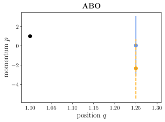
Figure 1: Initial state $(q_{k},p_{k})^{\top}$ (black dot) and image of the update function $\mathcal{U}_{\mathrm{ABO}}(\eta_{k};x_{k},V)$ for an unscaled potential (blue line) and a scaled potential (orange line) for the ABO method. The image of the update function contains all possible states $(q_{k+1},p_{k+1})^{\top}$ that can be reached from $(q_{k},p_{k})^{\top}$ within one integration time step $\Delta t$.
Parameters: $k_{B},m,T,\xi=1$, $\Delta t=0.25$, $(q_{k},p_{k})^{\top}=(1,1)^{\top}$, $V(q)=(q^{2}-1)^{2}+q$, $\widetilde{V}(q)=4.2\cdot(q^{2}-1)^{2}+q$ and $\eta\in[-5,5]$.

First, we consider Langevin integrators that use a single random number per integration step, i.e. one $\mathcal{O}$-step (eq. 35u) per integration step $k$. In Tab. 1, these are ABO, ABOBA, BAOAB and BAOA/GSD.

The following realization is crucial: given an initial state $x_{k}$, the image of $\mathcal{U}$ is not the entire state space $\Gamma$, but a one-dimensional curve $C_{1d}$ within $\Gamma$. This one-dimensional curve is parametrized by $\eta_{k}$. Formally, we can characterize the function $\mathcal{U}$ as

$$\mathcal{U}:\;\;\mathbb{R} \rightarrow C_{1d}\subset\Gamma$$ (62)

$$\mathcal{U}:\;\eta_{k} \mapsto x_{k+1}\,.$$ (63)

See Ref. 82 for an overview of parametrized curves and parametric equations.

Mathematically, it is not surprising that the image is one-dimensional, since it is impossible to map the one-dimensional number line $\mathbb{R}$ to a two-dimensional space. Algorithmically this means that, given an initial state $x_{k}$, not all states in state space $\Gamma$ can be reached by a single iteration of the integrator. Rather, the accessible states lie on $C_{1d}$, and which precise point on this line is obtained depends on $\eta_{k}$.

For the ABO method, this parametrization of $C_{1d}$ by $\eta_{k}$ can be made explicit by reformulating eq. 61 as

$$\left(\begin{array}[]{c}q_{k+1}\\ p_{k+1}\end{array}\right) = \mathcal{U}_{\mathrm{ABO}}(\eta_{k};x_{k},V)=\left(\begin{array}[]{l}q_{k+1}\\ \bar{p}_{k+1}\end{array}\right)+\left(\begin{array}[]{l}0\\ f\end{array}\right)\eta_{k}$$ (70)

with $q_{k+1}=q_{k}+ap_{k}$ and $\bar{p}_{k+1}=dp_{k}+db(q_{k}+ap_{k})$. That is, the algorithm first moves the system to $(q_{k+1},\bar{p}_{k+1})^{\top}$ and then adjusts the momenta by $(0,f)^{\top}\eta_{k}$. Consequently, all accessible states of $\mathcal{U}_{\mathrm{ABO}}(\eta_{k};x_{k},V)$ lie on a vertical through $(q_{k+1},\bar{p}_{k+1})^{\top}$.

Fig. 1 illustrates the image of $\mathcal{U}_{\mathrm{ABO}}(\eta_{k};x_{k},V)$. The initial point $(q_{k},p_{k})=(1,1)$ is marked as a black dot. The point $(q_{k+1},\bar{p}_{k+1})^{\top}$ for the potential $V(q)=(q^{2}-1)^{2}+q$ is shown as a blue dot and acts as the support point for the image of $\mathcal{U}_{\mathrm{ABO}}(\eta_{k};x_{k},V).$ Varying $\eta_{k}$ from -5 to +5 then yields the blue line, i.e. the image of $\mathcal{U}_{\mathrm{ABO}}(\eta_{k};x_{k},V)$ for $\eta_{k}\in[-5,5]$. When the potential is changed to $\widetilde{V}(q)=4.2\cdot(q^{2}-1)^{2}+q$, the point $(q_{k+1},\bar{p}_{k+1})^{\top}$ shifts to the orange point. Varying $\eta_{k}$ from -5 to +5 yields the image of $\mathcal{U}_{\mathrm{ABO}}(\eta_{k};x_{k},\widetilde{V})$ for $\eta_{k}\in[-5,5]$, shown as the dashed orange line in Fig. 1. For arbitrary values of $\eta_{k}$, the images of the two functions coincide. Thus, the image of the update function of the ABO method, i.e. the set of possible updated states $(q_{k+1},p_{k+1})$, does not depend on the potential $V$.

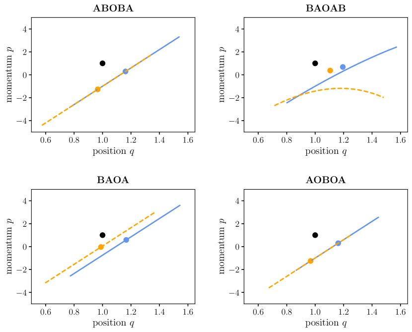
Figure 2: Initial state $(q_{k},p_{k})^{\top}$ (black dot) and image of the update function $\mathcal{U}(\eta_{k};x_{k},V)$ for an unscaled potential (blue line) and a scaled potential (orange line) for the ABOBA, BAOAB, BAOA/GSD and AOBOA method. The image of the update function contains all possible states $(q_{k+1},p_{k+1})^{\top}$ that can be reached from $(q_{k},p_{k})^{\top}$ within one integration time step $\Delta t$.
Parameters: $k_{B},m,T,\xi=1$, $\Delta t=0.25$, $(q_{k},p_{k})^{\top}=(1,1)^{\top}$, $V(q)=(x^{2}-1)^{2}+x$, $\widetilde{V}(q)=4.2\cdot(x^{2}-1)^{2}+x$, $\eta\in[-5,5]$, or $\eta^{\mathrm{comb}}\in[-5,5]$ .

The update functions for ABOBA, BAOAB and BAOA/GSD are derived in the supplementary material. Their images are summarized in the second column of Tab. 1 and illustrated in Fig. 2. As in Fig. 1, the current state $(q_{k},p_{k})$ is shown as a black dot, the support points for the image for two different potentials are shown as blue and orange dots, and the corresponding images for $\eta_{k}\in[-5,+5]$ are shown as blue and orange lines. Fig. 2 also contains the diagram for a Langevin integrator with two random numbers, AOBOA, which will be discussed in the following section.

Two aspects of the images of the update functions in Fig. 2 are important to point out. First, for ABOBA, BAOA/GSD and AOBOA, the possible updated states depend linearly on $\eta_{k}$, and thus the image is a line $L_{1d}$ in the state space $\Gamma$. By contrast, the possible updated states of BAOAB depend non-linearly on $\eta_{k}$, and the image is a curve $C_{1d}$. Second, in ABOBA and AOBOA the image does not depend on the potential, whereas in BAOAB and BAOA/GSD the image changes if $V$ is varied.

IV.2 Two random numbers per integration time step

Next, we consider Langevin integrators that generate two random numbers per integration step, i.e. two $\mathcal{O}$-half-steps (eq. 35u with $\Delta t/2$ instead of $\Delta t$) per integration step $k$. In Tab. 1, these are AOBOA, BOAOB, OBABO/BP, and OABAO. Their update functions are derived in the supplementary material.

The image of update functions of Langevin integrators with two random numbers can be the entire phase space $\Gamma$. That is, given an initial state $(q_{k},p_{k})$, any point in phase space can be reached within a single integration time step, albeit mostly with very low probability. For BOAOB and OBABO/BP this is indeed the case. Both of their update functions have the following form

$$\left(\begin{array}[]{c}q_{k+1}\\ p_{k+1}\end{array}\right) = \left(\begin{array}[]{l}\bar{q}_{k+1}\\ \bar{p}_{k+1}\end{array}\right)+\left(\begin{array}[]{l}0\\ c\cdot b^{\prime}(\bar{q}_{k+1}+af^{\prime}\eta_{k}^{(1)})\end{array}\right)+\left(\begin{array}[]{l}af^{\prime}\\ d^{\prime}f^{\prime}\end{array}\right)\eta_{k}^{(1)}+\left(\begin{array}[]{l}0\\ f^{\prime}\end{array}\right)\eta_{k}^{(2)}\,,$$ (81)

where $\eta_{k}^{(1)}$ and $\eta_{k}^{(2)}$ are the two random numbers, and $c=1$ for BOAOB, and $c=d^{\prime}$ for OBABO/BP. The functions first move the system deterministically to a support point $(\bar{q}_{k+1},\bar{p}_{k+1})$. BOAOB and OBABO/BP differ in the way this deterministic update is calculated (see supplementary material), but have analogous subsequent terms in the update function. (BOAOB: $\bar{q}_{k+1}=q_{k}+ad^{\prime}p_{k}+ad^{\prime}b^{\prime}(q_{k})$ and $\bar{p}_{k+1}=d^{\prime}d^{\prime}p_{k}+d^{\prime}d^{\prime}b^{\prime}(q_{k})$. OBABO/BP: $\bar{q}_{k+1}=q_{k}+ad^{\prime}p_{k}+ab^{\prime}(q_{k})$ and $\bar{p}_{k+1}=d^{\prime}d^{\prime}p_{k}+d^{\prime}b^{\prime}(q_{k})$.) From the support point, the momentum is slightly adjusted in the second term eq. 81, which however depends on the random number $\eta_{k}^{(1)}$ and thus represents a partly randomized update of the momentum. The last two terms in eq. 81 randomize the position and the momentum. Note that by scaling $\eta_{k}^{(1)}$ between $-\infty$ and $+\infty$, one can access any position, and by scaling $\eta_{k}^{(2)}$ one can access any momentum. Thus, the image of the update functions of BOAOB and OBABO/BP is the entire phase space $\Gamma$ (Tab. 1).

The update function of OABAO differs in a crucial point from eq. 81: in the second term both position and the momentum get a partly randomized update. This partly randomized update depends on the potential energy function via $b(q)$. One can construct cases, in which the update of the positions in the second term and the update in the third term compensate each other, and the images collapses from $\Gamma$ to a line (see supplementary material). Thus, the image of the update function of OABAO depends on the potential, and the existence of $M[\mathbf{x}|x_{0}]$ and analytical expressions for $\Delta\eta_{k}^{(1)}$ and $\Delta\eta_{k}^{(2)}$ need to be discussed in the context of specific potentials $V$ and $\widetilde{V}$. We will therefore exclude OABAO from the subsequent analysis.

AOBOA generates two random numbers $\eta_{k}^{(1)}$ and $\eta_{k}^{(2)}$ per integration time step. But $\eta_{k}^{(1)}$ and $\eta_{k}^{(2)}$ do not affect the position and the momentum independently as in eq. 81, and several combinations of $\eta_{k}^{(1)}$ and $\eta_{k}^{(2)}$ lead to the same updated state $(q_{k+1},p_{k+1})$. In fact, one can combine $\eta_{k}^{(1)}$ and $\eta_{k}^{(2)}$ into an effective random number

$$\eta^{\mathrm{comb}}_{k} = d^{\prime}\eta_{k}^{(1)}+\eta_{k}^{(2)}\sim\mathcal{N}(0,d^{\prime 2}+1)\,.$$ (82)

and formulate the update function in terms of $\eta^{\mathrm{comb}}_{k}$

$$\left(\begin{array}[]{c}q_{k+1}\\ p_{k+1}\end{array}\right) = \left(\begin{array}[]{l}\bar{q}_{k+1}\\ \bar{p}_{k+1}\end{array}\right)+\left(\begin{array}[]{l}a^{\prime}\\ 1\end{array}\right)f^{\prime}\eta^{\mathrm{comb}}$$ (89)

with $\bar{q}_{k+1}=q_{k}+(a^{\prime}+a^{\prime}d^{\prime}d^{\prime})p_{k}+a^{\prime}d^{\prime}b(q_{k}+a^{\prime}p_{k})$ and $\bar{p}_{k+1}=d^{\prime}d^{\prime}p_{k}+d^{\prime}b(q_{k}+a^{\prime}p_{k})$ (see supplementary material). The AOBOA method first generates a deterministic update and moves the system to the support point $(\bar{q}_{k+1},\bar{p}_{k+1})$, and then randomizes the position and momentum along a line with slope $(a^{\prime},1)$. Thus, the image of this update function is a line $L_{1d}$ through the state space $\Gamma$ (see Fig. 2). Note that any combination of $\eta_{k}^{(1)}$ and $\eta_{k}^{(2)}$ that yields the same value $\eta^{\mathrm{comb}}_{k}$, will yield the same updated state $(q_{k+1},p_{k+1})$.

		image at	absolute	reweighting in
integrator	update $u$	$V$ and $\widetilde{V}$	continuity	phase space
ABO	$\mathbb{R}\rightarrow L_{1d}$	$L_{1d}=\widetilde{L}_{1d}$	yes	$\Delta\eta_{k}=\frac{d}{f}\Delta t\nabla U(q_{k+1})$
ABOBA	$\mathbb{R}\rightarrow L_{1d}$	$L_{1d}=\widetilde{L}_{1d}$	yes	$\Delta\eta_{k}=\frac{(d+1)}{f}\frac{\Delta t}{2}\nabla U(q_{k+1/2})$
BAOAB	$\mathbb{R}\rightarrow C_{1d}$	$C_{1d}\neq\widetilde{C}_{1d}$	no	n/a
BAOA/GSD	$\mathbb{R}\rightarrow L_{1d}$	$L_{1d}\neq\widetilde{L}_{1d}$	no	n/a
AOBOA	$\mathbb{R}^{2}\rightarrow L_{1d}$	$L_{1d}=\widetilde{L}_{1d}$	yes	$\Delta\eta^{\mathrm{comb}}_{k}=\frac{d^{\prime}}{f^{\prime}}\Delta t\nabla U(q_{k+1/2})$
				$\eta^{\mathrm{comb}}_{k}=d^{\prime}\eta_{k}^{(1)}+\eta_{k}^{(2)}$
BOAOB	$\mathbb{R}^{2}\rightarrow\Gamma$	$\Gamma$ in both cases	yes	$\Delta\eta_{k}^{(1)}=\frac{d^{\prime}}{f^{\prime}}\,\frac{\Delta t}{2}\nabla U(q_{k})$
				$\Delta\eta_{k}^{(2)}=\frac{1}{f^{\prime}}\frac{\Delta t}{2}\nabla U(q_{k+1})$
OBABO/BP	$\mathbb{R}^{2}\rightarrow\Gamma$	$\Gamma$ in both cases	yes	$\Delta\eta_{k}^{(1)}=\frac{1}{f^{\prime}}\frac{\Delta t}{2}\nabla U(q_{k})$
				$\Delta\eta_{k}^{(2)}=\frac{d^{\prime}}{f^{\prime}}\,\frac{\Delta t}{2}\nabla U(q_{k+1})$
OABAO	depends on $V$ and $\widetilde{V}$.

Table 1: Image of integrator update function and corresponding expressions for the random number difference

V Absolute continuity and path reweighting factor

The notion of absolute continuity is closely related to the image of update function. Recall that absolute continuity implies that the same regions of path space are sampled by the dynamics at $\widetilde{V}(x)$ and by the dynamics at $V(x)$. If the image of the update function depends on the potential energy, transitions $(q_{k},p_{k})\rightarrow(q_{k+1},p_{k+1})$ that are possible at $V$ are impossible at $\widetilde{V}$. Thus, the corresponding path probabilities are not absolutely continuous with respect to each other, and $M[\mathbf{x}|x_{0}]$ does not exist for the corresponding integrators. Among the integrators we considered here, this is the case for BAOAB and BAOA/GSD (Tab. 1). Phase-space trajectories generated by these two integrators cannot be reweighted.

By contrast, the images of the update functions of ABO, ABOBA, AOBOA, BOAOB and OBABO/BP do no depend on the potential energy function. Consequently, any transition $(q_{k},p_{k})\rightarrow(q_{k+1},p_{k+1})$ that is possible at $V$ is also possible at $\widetilde{V}$. The corresponding path probabilities are absolutely continuous with respect to each other, and $M[\mathbf{x}|x_{0}]$ exists. Phase-space trajectories generated by these integrators can be reweighted (Tab. 1).

Having identified integrators of underdamped Langevin dynamics for which Girsanov reweighting is possible, we next derive computable expressions for $M[\mathbf{x}|x_{0}]$ using the reweighting-on-the-fly approach (eqs. 19 and 25). The mathematically formal way to derive an expression for $\Delta\eta_{k}=\widetilde{\eta}_{k}-\eta_{k}$ (eq. 18) goes as follows. We denote the update function of integrator $I$ at the simulation potential by $\mathcal{U}_{I}(\eta_{k};x_{k},V)$, and the update function of the same integrator at the target potential by $\mathcal{U}_{I}(\widetilde{\eta}_{k};x_{k},\widetilde{V})$. We require that both update operators yield the same update $(q_{k+1},p_{k+1})^{\top}$ given the initial state $x_{k}=(q_{k},p_{k})^{\top}$, i.e. the path remains unchanged,

$$\left(\begin{array}[]{c}q_{k+1}\\ p_{k+1}\end{array}\right) =\mathcal{U}_{I}(\eta_{k};x_{k},V)=\mathcal{U}_{I}(\widetilde{\eta}_{k};x_{k},\widetilde{V})\,.$$ (92)

Thus, we need to solve

$$\left(\begin{array}[]{l}0\\ 0\end{array}\right) =\mathcal{U}_{I}(\eta_{k};x_{k},V)-\mathcal{U}_{I}(\widetilde{\eta}_{k};x_{k},\widetilde{V})$$ (95)

for $\Delta\eta_{k}$, i.e. we determine the change in the random number that yields the same path even though the potential has changed.

V.1 One random number per integration time step

We again use the ABO method to illustrate how to derive an expression for $\Delta\eta_{k}$. Its update function at the simulation potential $V$ is eq. 61, and at the target potential $\widetilde{V}(q)$ it is

$$\left(\begin{array}[]{c}q_{k+1}\\ p_{k+1}\end{array}\right)=\mathcal{U}_{\mathrm{ABO}}(\widetilde{\eta}_{k};x_{k},\widetilde{V}) = \left(\begin{array}[]{l}q_{k}+ap_{k}\\ dp_{k}+d\widetilde{b}(q_{k}+ap_{k})+f\widetilde{\eta}_{k}\end{array}\right)\,,$$ (100)

where

$$\widetilde{b}(q) = b(q)-\Delta t\nabla U(q)\,.$$ (101)

Inserting eq. 61 and 100 into eq. 95 yields

$$\left(\begin{array}[]{c}0\\ 0\end{array}\right) = \mathcal{U}_{\mathrm{ABO}}(\eta_{k};x_{k},V)-\mathcal{U}_{\mathrm{ABO}}(\widetilde{\eta}_{k};x_{k},\widetilde{V})$$ (104)

$$= \left(\begin{array}[]{l}0\\ d\cdot(b(q_{k}+ap_{k})-\widetilde{b}(q_{k}+ap_{k}))+f\cdot(\eta_{k}-\widetilde{\eta}_{k})\end{array}\right)$$ (107)

$$= \left(\begin{array}[]{l}0\\ d\Delta t\nabla U(q_{k+1})-f\cdot\Delta\eta_{k}\end{array}\right)\,,$$ (110)

where, in the last line, we replaced $q_{k}+ap_{k}$ by $q_{k+1}$ (eq. 44a). Thus, for

$$\Delta\eta_{k} = \frac{d}{f}\Delta t\nabla U(q_{k+1})\,,$$ (111)

the two update functions yield the same state $(q_{k+1},p_{k+1})^{\top}$.

The same calculation for ABOBA yields

$$\Delta\eta_{k} = \frac{(d+1)}{f}\frac{\Delta t}{2}\nabla U(q_{k+1/2})\,$$ (112)

(see supplementary material). The relative conditional path probability densities $M[\mathbf{x}|x_{0}]$ for these two integrators can now be calculated according to eq. 19.

V.2 Two random numbers per integration time step

The condition

$$\left(\begin{array}[]{l}0\\ 0\end{array}\right) = \mathcal{U}_{\mathrm{BOAOB}}(\eta_{k}^{(1)},\eta_{k}^{(2)};x_{k},V)-\mathcal{U}_{\mathrm{BOAOB}}(\widetilde{\eta}_{k}^{(1)},\widetilde{\eta}_{k}^{(2)};x_{k},\widetilde{V})$$ (115)

yields the random number differences for the BOAOB method

$$\Delta\eta_{k}^{(1)} = \frac{d^{\prime}}{f^{\prime}}\,\frac{\Delta t}{2}\nabla U(q_{k})$$ (116a)

$$\Delta\eta_{k}^{(2)} = \frac{1}{f^{\prime}}\frac{\Delta t}{2}\nabla U(q_{k+1})\,.$$ (116b)

Similarly, the condition

$$\left(\begin{array}[]{l}0\\ 0\end{array}\right) = \mathcal{U}_{\mathrm{OBABO}}(\eta_{k}^{(1)},\eta_{k}^{(2)};x_{k},V)-\mathcal{U}_{\mathrm{OBABO}}(\widetilde{\eta}_{k}^{(1)},\widetilde{\eta}_{k}^{(2)};x_{k},\widetilde{V})$$ (119)

yields the random number differences for the OBABO/BP method

$$\Delta\eta_{k}^{(1)} =\frac{1}{f^{\prime}}\frac{\Delta t}{2}\nabla U(q_{k})$$ (120a)

$$\Delta\eta_{k}^{(2)} =\frac{d^{\prime}}{f^{\prime}}\,\frac{\Delta t}{2}\nabla U(q_{k+1})\,.$$ (120b)

For both methods, the intermediate steps of this calculation are reported in the supplementary material. The relative conditional path probability densities $M[\mathbf{x}|x_{0}]$ for these two integrators can now be calculated according to eq. 25.

V.3 AOBOA: two random numbers, but one-dimensional image

The condition

$$\left(\begin{array}[]{l}0\\ 0\end{array}\right) = \mathcal{U}_{\mathrm{AOBOA}}(\eta_{k}^{\mathrm{comb}};x_{k},V)-\mathcal{U}_{\mathrm{AOBOA}}(\widetilde{\eta}_{k}^{\mathrm{comb}};x_{k},\widetilde{V})\,,$$ (123)

where $\mathcal{U}_{\mathrm{AOBOA}}(\eta_{k}^{\mathrm{comb}};x_{k},V)$ is given by eq. 89, yields the difference of the combined random number

$$\Delta\eta^{\mathrm{comb}}_{k} = \frac{d^{\prime}}{f^{\prime}}\Delta t\nabla U(q_{k+1/2})\,.$$ (124)

The intermediate steps of this calculation are reported in the supplementary material.

To reweight trajectories generated by the AOBOA integrator, we need to formulate $M[\mathbf{x}|x_{0}]$ as a function of the combined random numbers $\eta^{\mathrm{comb}}_{k}$. From the update function of AOBOA (eq. 89), it follows that the conditional path probability is

$$\mathcal{P}[\mathbf{x}|x_{0}] = \mathcal{P}[\bm{\eta}^{\mathrm{comb}}]=\frac{1}{\sqrt[n]{2(d^{\prime 2}+1)\pi}}\exp\left(-\sum_{k=0}^{n-1}\frac{\left(\eta_{k}^{\mathrm{comb}}\right)^{2}}{2(d^{\prime 2}+1)}\right)\,.$$ (125)

Note that the probability density of the weighted sum of two normally distributed random numbers is again a normal distribution with adjusted mean $\mu$ and variance $\sigma^{2}$. For the combined random number (eq. 82): $\mu^{\mathrm{comb}}=d^{\prime}\mu^{(1)}+\mu^{(2)}=0$ and $(\sigma^{\mathrm{comb}})^{2}=d^{\prime 2}(\sigma^{(1)})^{2}+(\sigma^{(2)})^{2}=d^{\prime 2}+1$. The relative conditional path probability density for AOBOA is

$$M[\mathbf{x}|x_{0}]=\frac{\mathcal{P}[\widetilde{\bm{\eta}}^{\mathrm{comb}}]}{\mathcal{P}[\bm{\eta}^{\mathrm{comb}}]} = \exp\left(-\sum_{k=0}^{n-1}\frac{\eta_{k}^{\mathrm{comb}}\cdot\Delta\eta_{k}^{\mathrm{comb}}}{d^{\prime 2}+1}\right)\cdot\exp\left(-\sum_{k=0}^{n-1}\frac{\left(\Delta\eta_{k}^{\mathrm{comb}}\right)^{2}}{2(d^{\prime 2}+1)}\right)\,.$$ (126)

The random numbers $\eta_{k}^{(1)}$ and $\eta_{k}^{(2)}$ are recorded during the simulation at $V$. The combined random number $\eta_{k}^{\mathrm{comb}}$ is calculated according to eq. 82, and the expression for $\Delta\eta_{k}^{\mathrm{comb}}$ is given by eq. 124.

VI Graphical representation of Langevin integrators

In this section, we introduce a graphical representation of splitting methods for Langevin integrators. This representation helps in reasoning why some methods have potential-independent images, and why others do not. It also shows which parts of the integration algorithm are affected by a change in the potential and how this influences $\Delta\eta_{k}$.

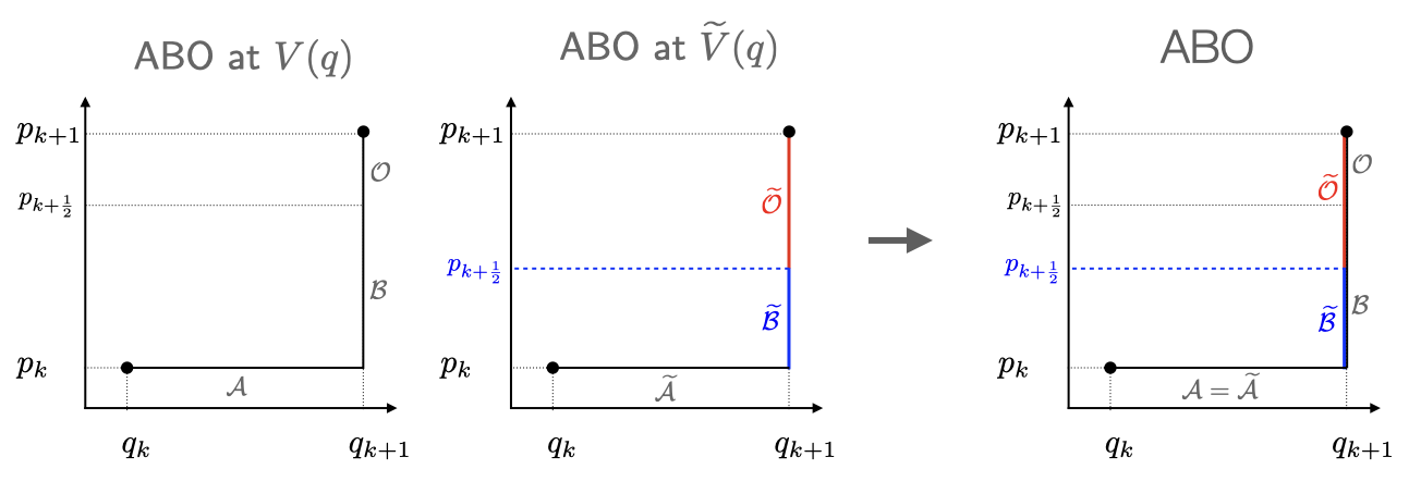
Figure 3: Update from $(q_{k},p_{k})$ to $(q_{k+1},p_{k+1})$ for the ABO method at the simulations potential $V(x)$ and at the target potential $\widetilde{V}(x)=V(x)+U(x)$. Update operators and intermediate results that are affected by the change in potential are shown in colour.

Fig. 3 illustrates this graphical representation for the ABO method. The graphs show the phase space $(q,p)$, and the black dots represent the initial state $(q_{k},p_{k})^{\top}$ and the state $(q_{k+1},p_{k+1})^{\top}$after one iteration of the ABO method. The left-hand graph shows the update from $(q_{k},p_{k})$ to $(q_{k+1},p_{k+1})$ for the simulation potential $V$ decomposed into the three update operators $\mathcal{A}$, $\mathcal{B}$, and $\mathcal{O}$. The $\mathcal{A}$-step depends on the momentum $p_{k}$ and updates the position from $q_{k}$ to $q_{k+1}$. This is followed by two momentum updates: the $\mathcal{B}$-step which depends on the updated position $q_{k+1}$ and potential $V$ and yields the intermediate momentum $p_{k+1/2}$, followed by an $\mathcal{O}$-step which depends on this intermediate momentum and a random number. The graph in the middle shows how the same update from $(q_{k},p_{k})$ to $(q_{k+1},p_{k+1})$ is achieved at the target potential. Update operators and intermediate results that are affected by the change in potential are shown in colour. The $\mathcal{A}$-step only depends on the initial momentum $p_{k}$ and therefore does not change. The $\mathcal{B}$-step evaluates the gradient of the potential and thus yields a different intermediate momentum $p_{k+1/2}$, shown in blue. In order to reach the state $(q_{k+1},p_{k+1})$, the random number in the $\mathcal{O}$-step needs to be adjusted such that $\mathcal{O}$ covers the remaining distance to $p_{k+1}$. Colloquially: we have to adjust the random number in the $\mathcal{O}$-step such that $\sqrt{k_{B}Tm(1-e^{-2\xi\Delta t})}\Delta\eta_{k}$ compensates “for the mess that $-\nabla U$ created”. The right-hand graph combines the two previous graphs, so that the update at $V(x)$ and at $\widetilde{V}(x)$ can be compared directly.

Because the $\mathcal{A}$-step in the ABO method is unaffected by a change in the potential, the equation to determine $\Delta\eta_{k}$ simplifies. Instead of the condition

$$\left[\mathcal{O}\mathcal{B}\mathcal{A}-\widetilde{\mathcal{O}}\widetilde{\mathcal{B}}\widetilde{\mathcal{A}}\right]\left(\begin{array}[]{l}q_{k}\\ p_{k}\end{array}\right) = \left(\begin{array}[]{c}0\\ 0\end{array}\right)$$ (131)

we only need to solve the condition

$$\left[\mathcal{O}\mathcal{B}-\widetilde{\mathcal{O}}\widetilde{\mathcal{B}}\right]\left(\begin{array}[]{c}q_{k+1}\\ p_{k}\end{array}\right) = \left(\begin{array}[]{c}0\\ 0\end{array}\right)\,.$$ (136)

which yields the same expression for $\Delta\eta_{k}$ as eq. 111.

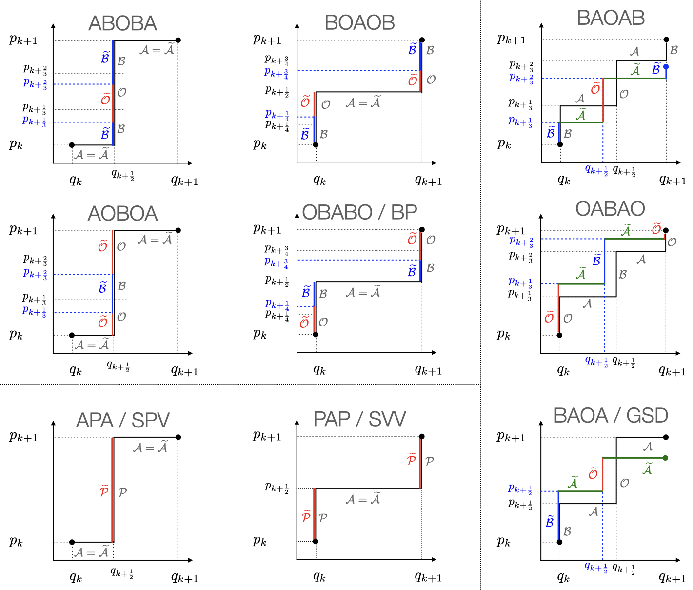
Figure 4: Decomposition of the transition from $(q_{k},p_{k})$ to $(q_{k+1},p_{k+1})$ for Langevin integrators derived via the operator splitting method. Methods that are not suited to reweight position trajectories are highlighted in gray.

Fig. 4 shows the graphical representation of the six symmetric splitting methods [46, 47, 48, 49]. as well as for BAOA/GSD. These Langevin integrators can be classified according to the route they take through phase space during an integration time step from $(q_{k},p_{k})$ to $(q_{k+1},p_{k+1})$. In the integrators in the first columns of Fig. 4, the position update occurs in two steps, and in between the steps the momentum is updated. Stochastic position Verlet (SPV) [68], a splitting method that has been proposed prior to the symmetric splitting methods, takes the same route through phase space. In the algorithm in the second column, the momentum update occurs in two steps, and in between the steps the position is updated. Also in this case, there is an older algorithm that takes the same route through phase space: stochastic velocity Verlet (SVV) [68]. Algorithms in which neither position nor momentum update is calculated in one go, but position and momentum update are interspersed, are shown in the third column.

Using Fig. 4, one can derive simplified conditions for $\Delta\eta_{k}$ by considering which sub-steps in the integrator are affected by a change in $V$. In the ABOBA method, the first $\mathcal{A}$-step depends only on $p_{k}$ and is not affected by a change in the potential. Therefore also the intermediate result $p_{k+1/2}$ is not affected by a change in the potential. The momentum update $p_{k}\rightarrow p_{k+1}$ is contained in the sequence of steps $\mathcal{BOB}$ (vertical line in Fig. 4), where the $\mathcal{B}$-step is affected by a change in the potential. In order to obtain the same momentum update in both potentials, the following condition for the two random numbers needs to be fulfilled:

$$\left[\mathcal{B^{\prime}}\mathcal{O}\mathcal{B}^{\prime}-\widetilde{\mathcal{B}^{\prime}}\widetilde{\mathcal{O}}\widetilde{\mathcal{B}^{\prime}}\right]\left(\begin{array}[]{c}q_{k+1/2}\\ p_{k}\end{array}\right) = \left(\begin{array}[]{c}0\\ 0\end{array}\right)$$ (141)

The final $\mathcal{A}$-step only depends on $p_{k+1}$ and is the same in both potentials if $p_{k+1}$ remains the same. Solving eq. 141 yields the same $\Delta\eta_{k}$ as defined in eq. 112. Similarly, in the AOBOA method it suffices to solve

$$\left[\mathcal{O^{\prime}}\mathcal{B}\mathcal{O}^{\prime}-\widetilde{\mathcal{O}^{\prime}}\widetilde{\mathcal{B}}\widetilde{\mathcal{O}^{\prime}}\right]\left(\begin{array}[]{c}q_{k+1/2}\\ p_{k}\end{array}\right) = \left(\begin{array}[]{c}0\\ 0\end{array}\right)$$ (146)

to obtain eq. 124 for $\Delta\eta_{k}^{\mathrm{cond}}$.

Consider the algorithms in the second column. In the BOAOB method, the update of the positions $q_{k}\rightarrow q_{k+1}$ is contained in a single $\mathcal{A}$-step, which depends on the intermediate momentum result $p_{k+1/2}$. If $p_{k+1/2}$ is altered, $q_{k+1}$ will change. In order to obtain the same path at the simulation and at the target potential, $p_{k+1/2}$ has to be the same in both potentials. This is the case, if the updates $p_{k}\rightarrow p_{k+1/2}$ and $p_{k+1/2}\rightarrow p_{k+1}$ (vertical lines in Fig. 4) are the same in both potentials. Thus, we have two separate conditions, one for each random number:

$$\left[\mathcal{O}^{\prime}\mathcal{B}^{\prime}-\widetilde{\mathcal{O}^{\prime}}\widetilde{\mathcal{B}^{\prime}}\right]\left(\begin{array}[]{c}q_{k}\\ p_{k}\end{array}\right) = \left(\begin{array}[]{c}0\\ 0\end{array}\right)$$ (147e)

$$\left[\mathcal{B}^{\prime}\mathcal{O}^{\prime}-\widetilde{\mathcal{B}^{\prime}}\widetilde{\mathcal{O}^{\prime}}\right]\left(\begin{array}[]{c}q_{k+1}\\ p_{k+1/2}\end{array}\right) = \left(\begin{array}[]{c}0\\ 0\end{array}\right)$$ (147j)

which lead to eqs. 116a and 116b for $\eta_{k}^{(1)}$ and $\eta_{k}^{(2)}$. (Note that the operators act from right to left, and thus their order is reversed compared to the name of the method.) Similarly, the conditions for OBABO/BP are

$$\left[\mathcal{B}^{\prime}\mathcal{O}^{\prime}-\widetilde{\mathcal{B}^{\prime}}\widetilde{\mathcal{O}^{\prime}}\right]\left(\begin{array}[]{c}q_{k}\\ p_{k}\end{array}\right) = \left(\begin{array}[]{c}0\\ 0\end{array}\right)$$ (148e)

$$\left[\mathcal{O}^{\prime}\mathcal{B}^{\prime}-\widetilde{\mathcal{O}^{\prime}}\widetilde{\mathcal{B}^{\prime}}\right]\left(\begin{array}[]{c}q_{k+1}\\ p_{k+1/2}\end{array}\right) = \left(\begin{array}[]{c}0\\ 0\end{array}\right)$$ (148j)

which lead to eqs. 120a and 120b for $\eta_{k}^{(1)}$ and $\eta_{k}^{(2)}$.

BAOAB and BAOA/GSD in the third column in Fig. 4 do not allow for reweighting in phase space. Consider BAOA/GSD to understand why. The first two steps in the algorithm are deterministic and the $\mathcal{B}$-step is affected by a change in $V$. Consequently, at $\widetilde{V}$ the intermediate state $(q_{k+1/2},p_{k+1/2})$ will be different from the intermediate state at $V$. One can now choose the value of $\eta_{k}$ such that the $\mathcal{O}$-step reaches $p_{k+1}$. In that case, the subsequent $\mathcal{A}$-step will not reach $q_{k+1}$. Or one can scale to a momentum $\widetilde{p}_{k+1}$ that is sufficient to bridge the remaining gap between $q_{k+1/2}$ and $q_{k+1}$, but this $\widetilde{p}_{k+1}$ will not be equal to the original $p_{k+1}$. Thus, one can reach either $p_{k+1}$ or $q_{k+1}$, but not both. The equations for the corresponding values of $\Delta\eta_{k}$ are reported in the supplementary material. Note that this in principles allows for reweighting path expected values, in which the path observable $s[\mathbf{x}]$ only depends on the positions or only depends on the momenta. However, the resulting reweighted estimators might have a large variance or even a bias. An analogous reasoning applies to BAOAB. We provide the equations for $\Delta\eta_{k}$ for separately reweighting in position and momentum space in the supplementary material, and give the same warning. For the OBABO method reweighting should in principle be possible, because we have two random numbers to adjust the updated position and the updated momentum. However, since pathological cases in which the image of the update function changes with the potential can be constructed (see supplementary material), we do not derive the equations for the random number differences here.

VII Conclusion

We have introduced a strategy to derive the relative path-probability ratio for Langevin integrators. To achieve this, we adapted the method to derive the random number difference $\Delta\eta_{k}$ as presented in Ref. 45. With the random numbers differences presented in Tab. 1 it is now possible to use Girsanov reweighting with underdamped Langevin dynamics. This removes a major road block to study rare events by combining biased simulations with dynamical reweighting.

Besides reweighting enhanced sampling simulations, the relative path probability ratio for underdamped Langevin integrators can also be use in other contexts such as searching and sampling in path space [83, 84, 85] or force-field optimization [86]. It might also help in understanding the relation between molecular models that rely on path sampling and models that are derived from a direct discretization of the Fokker-Planck equation [78].

The analysis revealed that some algorithms violate absolute continuity, because the image of their update changes when the potential is change. As a consequence single-step transitions $(q_{k},p_{k})\rightarrow(q_{k+1},p_{k+1})$ that are possible at the simulation potential are no longer possible at the target potential. Our condition for the absolute continuity of the single-step transitions (eq. 15) is a very strict condition and guarantees the Girsanov reweighting in the full phase space is possible. However, path observables usually either depend on the positions or on the momenta, rarely on both. Thus, for algorithms that violate eq. 15 reweighting in position space or in path space might still be possible. In fact, we report random number difference for these approaches for BAOA/GSD in the supplementary material. Whether these equations yield accurate results has yet to be tested. Another interesting question is how the absolute continuity of a Langevin integrator relates to the accuracy with which it reproduces transport properties [74, 75]. Finally, in some cases one might be able to relax the absolute continuity over a single integration time-step to an absolute continuity over a larger lag time of several integration time steps, and thereby link Girsanov reweighting to dynamical reweighting methods that assume a Markov state model [20, 21, 22, 23, 24].

VIII Acknowledgements

This research has been funded by Deutsche Forschungsgemeinschaft (DFG) through grant SFB 1114 ”Scaling Cascades in Complex Systems” - project number 235221301, and through grant GRK 2473 ”Bioactive Peptides” - project number 392923329. S.G. acknowledges funding by the Einstein Center of Catalysis/BIG-NSE.

IX References

Appendix A Langevin integration methods

For the update operators we use the following abbreviations:

$$a = \Delta t\frac{1}{m}$$ (149a)

$$b(q_{k}) = -\Delta t\nabla V(q_{k})$$ (149b)

$$d = e^{-\xi\Delta t}$$ (149c)

$$f = \sqrt{k_{B}Tm(1-e^{-2\xi\Delta t})}\,.$$ (149d)

and for half time steps

$$a^{\prime} = \frac{\Delta t}{2}\frac{1}{m}$$ (150a)

$$b^{\prime}(q_{k}) = -\frac{\Delta t}{2}\nabla V(q_{k})$$ (150b)

$$d^{\prime} = e^{-\xi\frac{\Delta t}{2}}$$ (150c)

$$f^{\prime} = \sqrt{k_{B}Tm(1-e^{-2\xi\frac{\Delta t}{2}})}\,.$$ (150d)

We will further use that

$$\widetilde{\eta_{k}}-\eta_{k} = \Delta\eta_{k}$$ (151)

and that

$$\widetilde{b}(q_{k})-b(q_{k}) = -\Delta t\nabla\widetilde{V}(q_{k})+\Delta t\nabla V(q_{k})$$ (152)

$$= -\Delta t(\nabla V(q_{k})+\nabla U(q_{k}))+\Delta t\nabla V(q_{k})$$ (153)

$$= -\Delta t\nabla U(q_{k})\,$$ (154)

and analogously for half-time steps.

A.1 ABOBA

A.1.1 Algorithm

$$q_{k+1/2} = q_{k}+\frac{\Delta t}{2m}p_{k}$$ (155a)

$$p_{k+1/3} = p_{k}-\frac{\Delta t}{2}\nabla V(q_{k+1/2})$$ (155b)

$$p_{k+2/3} = e^{-\xi\Delta t}p_{k+1/3}+\sqrt{k_{B}Tm(1-e^{-2\xi\Delta t})}\,\eta_{k}$$ (155c)

$$p_{k+1} = p_{k+2/3}-\frac{\Delta t}{2}\,\nabla V(q_{k+1/2})$$ (155d)

$$q_{k+1} = q_{k+1/2}+\frac{\Delta t}{2m}\,p_{k+1}$$ (155e)

The algorithm has been reported in Refs. 47 and in 57. Compared to Ref. 48, we changed the notation as follows: $n\rightarrow k$, $R_{n}\rightarrow\eta_{k}$, $\delta t\rightarrow\Delta t$, $M\rightarrow m$, $\gamma\rightarrow\xi$, $F\rightarrow-\nabla V$.

A.1.2 Update operator

$$\mathcal{A^{\prime}B^{\prime}OB^{\prime}A^{\prime}}\left(\begin{array}[]{l}q_{k}\\ p_{k}\end{array}\right) = \mathcal{A^{\prime}B^{\prime}OB^{\prime}}\left(\begin{array}[]{l}q_{k}+a^{\prime}p_{k}\\ p_{k}\end{array}\right)$$ (160)

$$= \mathcal{A^{\prime}B^{\prime}O}\left(\begin{array}[]{l}q_{k}+a^{\prime}p_{k}\\ p_{k}+b^{\prime}(q_{k}+a^{\prime}p_{k})\end{array}\right)$$ (163)

$$= \mathcal{A^{\prime}B^{\prime}}\left(\begin{array}[]{l}q_{k}+a^{\prime}p_{k}\\ dp_{k}+db^{\prime}(q_{k}+a^{\prime}p_{k})+f\eta_{k}\end{array}\right)$$ (166)

$$= \mathcal{A^{\prime}}\left(\begin{array}[]{l}q_{k}+a^{\prime}p_{k}\\ dp_{k}+db^{\prime}(q_{k}+a^{\prime}p_{k})+f\eta_{k}+b^{\prime}(q_{k}+a^{\prime}p_{k})\end{array}\right)$$ (169)

$$= \left(\begin{array}[]{l}q_{k}+a^{\prime}p_{k}+a^{\prime}[dp_{k}+db^{\prime}(q_{k}+a^{\prime}p_{k})+f\eta_{k}+b^{\prime}(q_{k}+a^{\prime}p_{k})]\\ dp_{k}+db^{\prime}(q_{k}+a^{\prime}p_{k})+f\eta_{k}+b^{\prime}(q_{k}+a^{\prime}p_{k})\end{array}\right)$$ (172)

A.1.3 Update function

$$\left(\begin{array}[]{c}q_{k+1}\\ p_{k+1}\end{array}\right)=\mathcal{U}_{\mathrm{ABOBA}}(\eta_{k};x_{k},V) = \left(\begin{array}[]{l}\bar{q}_{k+1}\\ \bar{p}_{k+1}\end{array}\right)+\left(\begin{array}[]{l}a^{\prime}f\\ f\end{array}\right)\eta_{k}$$ (179)

with $\bar{q}_{k+1}=q_{k}+a^{\prime}(1+d)p_{k}+a^{\prime}(d+1)b^{\prime}(q_{k}+a^{\prime}p_{k})$ and $\bar{p}_{k+1}=dp_{k}+(d+1)b^{\prime}(q_{k}+a^{\prime}p_{k})$. Thus,

$$\mathcal{U}_{\mathrm{ABOBA}}:\;\;\mathbb{R} \rightarrow L_{1d}\subset\Gamma$$ (180)

$$\mathcal{U}_{\mathrm{ABOBA}}:\;\eta_{k} \mapsto x_{k+1}\,,$$ (181)

where $L_{1d}$ denotes a line in $\Gamma$.

A.1.4 Image at $V$ and $\widetilde{V}$

$$\left(\begin{array}[]{c}0\\ 0\end{array}\right) = \mathcal{U}_{\mathrm{ABOBA}}(\eta_{k};x_{k},V)-\mathcal{U}_{\mathrm{ABOBA}}(\widetilde{\eta_{k}};x_{k},\widetilde{V})$$ (184)

$$= \left(\begin{array}[]{l}q_{k}+a^{\prime}p_{k}+a^{\prime}(dp_{k}+db^{\prime}(q_{k}+a^{\prime}p_{k})+f\eta_{k}+b^{\prime}(q_{k}+a^{\prime}p_{k}))\\ dp_{k}+db^{\prime}(q_{k}+a^{\prime}p_{k})+f\eta_{k}+b^{\prime}(q_{k}+a^{\prime}p_{k})\end{array}\right)-$$ (190)

$$\left(\begin{array}[]{l}q_{k}+a^{\prime}p_{k}+a^{\prime}(dp_{k}+d\widetilde{b}^{\prime}(q_{k}+a^{\prime}p_{k})+f\widetilde{\eta}_{k}+\widetilde{b}^{\prime}(q_{k}+a^{\prime}p_{k}))\\ dp_{k}+d\widetilde{b}^{\prime}(q_{k}+a^{\prime}p_{k})+f\widetilde{\eta}_{k}+\widetilde{b}^{\prime}(q_{k}+a^{\prime}p_{k})\end{array}\right)$$

$$= \left(\begin{array}[]{l}a^{\prime}[d\cdot b^{\prime}(q_{k}+a^{\prime}p_{k})+f\eta_{k}+b^{\prime}(q_{k}+a^{\prime}p_{k})]\\ db^{\prime}(q_{k}+a^{\prime}p_{k})+f\eta_{k}+b^{\prime}(q_{k}+a^{\prime}p_{k})\end{array}\right)-$$ (196)

$$\left(\begin{array}[]{l}a^{\prime}[d\cdot\widetilde{b}^{\prime}(q_{k}+a^{\prime}p_{k})+f\widetilde{\eta}_{k}+\widetilde{b}^{\prime}(q_{k}+a^{\prime}p_{k})]\\ d\widetilde{b}^{\prime}(q_{k}+a^{\prime}p_{k})+f\widetilde{\eta}_{k}+\widetilde{b}^{\prime}(q_{k}+a^{\prime}p_{k})\end{array}\right)$$

$$= \left(\begin{array}[]{l}a^{\prime}\\ 1\end{array}\right)[d\cdot b^{\prime}(q_{k}+a^{\prime}p_{k})+f\eta_{k}+b^{\prime}(q_{k}+a^{\prime}p_{k})]-$$ (202)

$$\left(\begin{array}[]{l}a^{\prime}\\ 1\end{array}\right)[d\cdot\widetilde{b}^{\prime}(q_{k}+a^{\prime}p_{k})+f\widetilde{\eta}_{k}+\widetilde{b}^{\prime}(q_{k}+a^{\prime}p_{k})]$$

$$= \left(\begin{array}[]{l}a^{\prime}\\ 1\end{array}\right)[d\cdot b^{\prime}(q_{k}+a^{\prime}p_{k})+f\eta_{k}+b^{\prime}(q_{k}+a^{\prime}p_{k})-d\cdot\widetilde{b}^{\prime}(q_{k}+a^{\prime}p_{k})-f\widetilde{\eta}_{k}-\widetilde{b}^{\prime}(q_{k}+a^{\prime}p_{k})]$$ (205)

$$= \left(\begin{array}[]{l}a^{\prime}\\ 1\end{array}\right)[(d+1)\cdot b^{\prime}(q_{k}+a^{\prime}p_{k})-(d+1)\cdot\widetilde{b}^{\prime}(q_{k}+a^{\prime}p_{k})+f(\eta_{k}-\widetilde{\eta}_{k})]$$ (208)

$$= \left(\begin{array}[]{l}a^{\prime}\\ 1\end{array}\right)[(d+1)\cdot\frac{\Delta t}{2}\nabla U(q_{k+1/2})-f\Delta\eta_{k}]$$ (211)

is fulfilled if

$$\Delta\eta_{k} = \frac{(d+1)}{f}\frac{\Delta t}{2}\nabla U(q_{k+1/2})\,,$$ (212)

where we substituted $q_{k+1/2}=q_{k}+a^{\prime}p_{k}$ (eq. 155a) and used eqs. LABEL:eq:fDeltaEta_k and eq. 154. Thus, $\mathcal{U}_{\mathrm{ABOBA}}(\eta_{k};x_{k},V)$ and $\mathcal{U}_{\mathrm{ABOBA}}(\widetilde{\eta_{k}};x_{k},\widetilde{V})$ have the same image

$$L_{1d}=\widetilde{L}_{1d}\,.$$

A.2 BAOAB

A.2.1 Algorithm

$$p_{k+1/3} = p_{k}-\frac{\Delta t}{2}\nabla V(q_{k})$$ (213a)

$$q_{k+1/2} = q_{k}+\frac{\Delta t}{2m}\,p_{k+1/3}$$ (213b)

$$p_{k+2/3} = e^{-\xi\Delta t}\,p_{k+1/3}+\sqrt{k_{B}Tm(1-e^{-2\xi\Delta t})}\,\eta_{k}$$ (213c)

$$q_{k+1} = q_{k+1/2}+\frac{\Delta t}{2m}\,p_{k+2/3}$$ (213d)

$$p_{k+1} = p_{k+2/3}-\frac{\Delta t}{2}\nabla V(q_{k+1})$$ (213e)

The algorithm has been reported in Refs. 47 and 57. Compared to Ref. 48, we changed the notation as follows: $n\rightarrow k$, $R_{n}\rightarrow\eta_{k}$, $\delta t\rightarrow\Delta t$, $M\rightarrow m$, $\gamma\rightarrow\xi$, $F\rightarrow-\nabla V$.

A.2.2 Update operator

$$\mathcal{B^{\prime}A^{\prime}OA^{\prime}B^{\prime}}\left(\begin{array}[]{l}q_{k}\\ p_{k}\end{array}\right) = \mathcal{B^{\prime}A^{\prime}OA^{\prime}}\left(\begin{array}[]{l}q_{k}\\ p_{k}+b^{\prime}(q_{k})\end{array}\right)$$ (218)

$$= \mathcal{B^{\prime}A^{\prime}O}\left(\begin{array}[]{l}q_{k}+a^{\prime}p_{k}+a^{\prime}b^{\prime}(q_{k})\\ p_{k}+b^{\prime}(q_{k})\end{array}\right)$$ (221)

$$= \mathcal{B^{\prime}A^{\prime}}\left(\begin{array}[]{l}q_{k}+a^{\prime}p_{k}+a^{\prime}b^{\prime}(q_{k})\\ dp_{k}+db^{\prime}(q_{k})+f\eta_{k}\end{array}\right)$$ (224)

$$= \mathcal{B^{\prime}}\left(\begin{array}[]{l}q_{k}+a^{\prime}p_{k}+a^{\prime}b^{\prime}(q_{k})+a^{\prime}dp_{k}+a^{\prime}db^{\prime}(q_{k})+a^{\prime}f\eta_{k}\\ dp_{k}+db^{\prime}(q_{k})+f\eta_{k}\end{array}\right)$$ (227)

$$= \left(\begin{array}[]{l}q_{k}+a^{\prime}p_{k}+a^{\prime}b^{\prime}(q_{k})+a^{\prime}dp_{k}+a^{\prime}db^{\prime}(q_{k})+a^{\prime}f\eta_{k}\\ dp_{k}+db^{\prime}(q_{k})+f\eta_{k}+b^{\prime}(q_{k}+a^{\prime}p_{k}+a^{\prime}b^{\prime}(q_{k})+a^{\prime}dp_{k}+a^{\prime}db^{\prime}(q_{k})+a^{\prime}f\eta_{k})\end{array}\right)$$ (230)

A.2.3 Update function

$$\left(\begin{array}[]{c}q_{k+1}\\ p_{k+1}\end{array}\right)=\mathcal{U}_{\mathrm{BAOAB}}(\eta_{k};x_{k},V) = \left(\begin{array}[]{l}\bar{q}_{k+1}\\ \bar{p}_{k+1}\end{array}\right)+\left(\begin{array}[]{l}0\\ b^{\prime}(\bar{q}_{k+1}+a^{\prime}f\eta_{k})\end{array}\right)+\left(\begin{array}[]{l}a^{\prime}f\\ f\end{array}\right)\eta_{k}$$ (239)

with $\bar{q}_{k+1}=q_{k}+a^{\prime}p_{k}+a^{\prime}b^{\prime}(q_{k})+a^{\prime}dp_{k}+a^{\prime}db^{\prime}(q_{k})=q_{k}+a^{\prime}(1+d)p_{k}+a^{\prime}(1+d)b^{\prime}(q_{k})$ and $\bar{p}_{k+1}=dp_{k}+db^{\prime}(q_{k})$. Thus,

$$\mathcal{U}_{\mathrm{BAOAB}}:\;\;\mathbb{R} \rightarrow C_{1d}\subset\Gamma$$ (240)

$$\mathcal{U}_{\mathrm{BAOAB}}:\;\eta_{k} \mapsto x_{k+1}\,,$$ (241)

where $C_{1d}$ denotes a curve in $\Gamma$.

A.2.4 Image at $V$ and $\widetilde{V}$

$$\left(\begin{array}[]{c}0\\ 0\end{array}\right) = \mathcal{U}_{\mathrm{BAOAB}}(\eta_{k};x_{k},V)-\mathcal{U}_{\mathrm{BAOAB}}(\widetilde{\eta_{k}};x_{k},\widetilde{V})$$ (244)

$$= \left(\begin{array}[]{l}q_{k}+a^{\prime}(1+d)p_{k}+a^{\prime}(1+d)b^{\prime}(q_{k})+a^{\prime}f\eta_{k}\\ dp_{k}+d\cdot b^{\prime}(q_{k})+f\eta_{k}+b^{\prime}(q_{k}+a^{\prime}(1+d)p_{k}+a^{\prime}(1+d)b^{\prime}(q_{k})+a^{\prime}f\eta_{k})\end{array}\right)-$$ (250)

$$\left(\begin{array}[]{l}q_{k}+a^{\prime}(1+d)p_{k}+a^{\prime}(1+d)\widetilde{b}^{\prime}(q_{k})+a^{\prime}f\widetilde{\eta}_{k}\\ dp_{k}+d\cdot\widetilde{b}^{\prime}(q_{k})+f\widetilde{\eta}_{k}+\widetilde{b}^{\prime}(q_{k}+a^{\prime}(1+d)p_{k}+a^{\prime}(1+d)\widetilde{b}^{\prime}(q_{k})+a^{\prime}f\widetilde{\eta}_{k})\end{array}\right)$$

$$= \left(\begin{array}[]{l}a^{\prime}(d+1)\cdot b^{\prime}(q_{k})+a^{\prime}f\eta_{k}\\ d\cdot b^{\prime}(q_{k})+b^{\prime}(q_{k}+a^{\prime}(d+1)p_{k}+a^{\prime}(d+1)\cdot b^{\prime}(q_{k})+a^{\prime}f\eta_{k})+f\eta_{k}\end{array}\right)-$$ (256)

$$\left(\begin{array}[]{l}a^{\prime}(d+1)\cdot\widetilde{b}^{\prime}(q_{k})+a^{\prime}f\widetilde{\eta}_{k}\\ d\cdot\widetilde{b}^{\prime}(q_{k})+\widetilde{b}^{\prime}(q_{k}+a^{\prime}(d+1)p_{k}+a^{\prime}(d+1)\cdot\widetilde{b}^{\prime}(q_{k})+a^{\prime}f\widetilde{\eta}_{k})+f\widetilde{\eta}_{k}\end{array}\right)\,.$$

$\eta_{k}$ appears linearly in the update of the positions. It appears as the argument of the function $b(q)$ in the update of the momenta which is typically a non-linear function (eq. 149b). Therefore, one cannot find an analytical expression for $\Delta\eta_{k}$ that solves both lines of the equation.

One can however find an expression for $\Delta\eta_{k}^{\mathrm{pos}}$, for which the two update functions yield the same positions:

$$0 = a^{\prime}(d+1)\cdot b^{\prime}(q_{k})+a^{\prime}f\eta_{k}-a^{\prime}(d+1)\cdot\widetilde{b}^{\prime}(q_{k})-a^{\prime}f\widetilde{\eta}_{k}$$ (257)

$$= a^{\prime}(d+1)\cdot\frac{\Delta t}{2}\nabla U(q_{k})-a^{\prime}f\Delta\eta_{k}^{\mathrm{pos}}$$ (258)

$$\Updownarrow$$ (259)

$$\Delta\eta_{k}^{\mathrm{pos}} = \frac{d+1}{f}\frac{\Delta t}{2}\nabla U(q_{k})\,.$$ (260)

Then

$$q_{k+1} = q_{k}+a^{\prime}(d+1)p_{k}+a^{\prime}(d+1)\cdot b^{\prime}(q_{k})+a^{\prime}f\eta_{k}$$ (261)

$$= q_{k}+a^{\prime}(d+1)p_{k}+a^{\prime}(d+1)\cdot\widetilde{b}^{\prime}(q_{k})+a^{\prime}f\widetilde{\eta}_{k}\,,$$ (262)

and we can make the following substitution in the equation above

$$\left(\begin{array}[]{c}0\\ 0\end{array}\right) = \left(\begin{array}[]{l}0\\ d\cdot b^{\prime}(q_{k})+b^{\prime}(q_{k+1})+f\eta_{k}-d\cdot\widetilde{b}^{\prime}(q_{k})-\widetilde{b}^{\prime}(q_{k+1})-f\widetilde{\eta}_{k}\end{array}\right)$$ (267)

$$= \left(\begin{array}[]{l}0\\ d\frac{\Delta t}{2}\nabla U(q_{k})+\frac{\Delta t}{2}\nabla U(q_{k+1})-f\Delta\eta_{k}^{\mathrm{pos}}\end{array}\right)\,.$$ (270)

One can now see that the equation for the momenta is not fulfilled, because

$$0 \neq d\frac{\Delta t}{2}\nabla U(q_{k})+\frac{\Delta t}{2}\nabla U(q_{k+1})-f\Delta\eta_{k}^{\mathrm{pos}}$$ (271)

$$0 \neq d\frac{\Delta t}{2}\nabla U(q_{k})+\frac{\Delta t}{2}\nabla U(q_{k+1})-(d+1)\frac{\Delta t}{2}\nabla U(q_{k})$$ (272)

$$\nabla U(q_{k+1}) \neq \nabla U(q_{k})\,.$$ (274)

Thus, $\mathcal{U}_{\mathrm{BAOAB}}(\eta_{k};x_{k},V)$ and $\mathcal{U}_{\mathrm{BAOAB}}(\widetilde{\eta_{k}};x_{k},\widetilde{V})$ parameterise different curves in state space

$$C_{1d}\neq\widetilde{C}_{1d}\,.$$

A.3 BAOA/ Gromacs stochastic dynamics

BAOA is equivalent to Gromacs stochastic dynamics (GSD)[52, 50].

A.3.1 Algorithm

$$p_{k+\frac{1}{2}} = p_{k}-\Delta t\nabla V(q_{k})$$ (275a)

$$q_{k+\frac{1}{2}} = q_{k}+\frac{\Delta t}{2m}p_{k+\frac{1}{2}}$$ (275b)

$$p_{k+1} = e^{-\xi\Delta t}p_{k+\frac{1}{2}}+\sqrt{k_{B}Tm\left(1-e^{-2\xi\Delta t}\right)}\eta_{k}$$ (275c)

$$q_{k+1} = q_{k+\frac{1}{2}}+\frac{\Delta t}{2m}p_{k+1}.$$ (275d)

A.3.2 Update operator

$$\mathcal{A^{\prime}OA^{\prime}B}\left(\begin{array}[]{l}q_{k}\\ p_{k}\end{array}\right) = \mathcal{A^{\prime}OA^{\prime}}\left(\begin{array}[]{l}q_{k}\\ p_{k}+b(q_{k})\end{array}\right)$$ (280)

$$= \mathcal{A^{\prime}O}\left(\begin{array}[]{l}q_{k}+a^{\prime}p_{k}+a^{\prime}b(q_{k})\\ p_{k}+b(q_{k})\end{array}\right)$$ (283)

$$= \mathcal{A^{\prime}}\left(\begin{array}[]{l}q_{k}+a^{\prime}p_{k}+a^{\prime}b(q_{k})\\ dp_{k}+db(q_{k})+f\eta_{k}\end{array}\right)$$ (286)

$$= \left(\begin{array}[]{l}q_{k}+a^{\prime}p_{k}+a^{\prime}b(q_{k})+a^{\prime}dp_{k}+a^{\prime}db(q_{k})+a^{\prime}f\eta_{k}\\ dp_{k}+db(q_{k})+f\eta_{k}\end{array}\right)$$ (289)

A.3.3 Update function

$$\left(\begin{array}[]{c}q_{k+1}\\ p_{k+1}\end{array}\right)=\mathcal{U}_{\mathrm{BAOA}}(\eta_{k};x_{k},V) = \left(\begin{array}[]{l}\bar{q}_{k+1}\\ \bar{p}_{k+1}\end{array}\right)+\left(\begin{array}[]{l}a^{\prime}f\\ f\end{array}\right)\eta_{k}$$ (296)

with $\bar{q}_{k+1}=q_{k}+a^{\prime}p_{k}+a^{\prime}b(q_{k})+a^{\prime}dp_{k}+a^{\prime}db(q_{k})=q_{k}+a^{\prime}(1+d)p_{k}+a^{\prime}(1+d)b(q_{k})$ and $\bar{p}_{k+1}=dp_{k}+db(q_{k})$. Thus,

$$\mathcal{U}_{\mathrm{BAOA}}:\;\;\mathbb{R} \rightarrow L_{1d}\subset\Gamma$$ (297)

$$\mathcal{U}_{\mathrm{BAOA}}:\;\eta_{k} \mapsto x_{k+1}\,,$$ (298)

where $L_{1d}$ denotes a line in $\Gamma$.

A.3.4 Image at $V$ and $\widetilde{V}$

$$\left(\begin{array}[]{c}0\\ 0\end{array}\right) = \mathcal{U}_{\mathrm{BAOA}}(\eta_{k};x_{k},V)-\mathcal{U}_{\mathrm{BAOA}}(\widetilde{\eta_{k}};x_{k},\widetilde{V})$$ (301)

$$= \left(\begin{array}[]{l}q_{k}+a^{\prime}(1+d)p_{k}+a^{\prime}(1+d)b(q_{k})+a^{\prime}f\eta_{k}\\ dp_{k}+d\cdot b(q_{k})+f\eta_{k}\end{array}\right)-$$ (307)

$$\left(\begin{array}[]{l}q_{k}+a^{\prime}(1+d)p_{k}+a^{\prime}(1+d)\widetilde{b}(q_{k})+a^{\prime}f\widetilde{\eta}_{k}\\ dp_{k}+d\cdot\widetilde{b}(q_{k})+f\widetilde{\eta}_{k}\end{array}\right)$$

$$= \left(\begin{array}[]{l}a^{\prime}(1+d)\cdot b(q_{k})+a^{\prime}f\eta_{k}\\ d\cdot b(q_{k})+f\eta_{k}\end{array}\right)-\left(\begin{array}[]{l}a^{\prime}(1+d)\cdot\widetilde{b}(q_{k})+a^{\prime}f\widetilde{\eta}_{k}\\ d\cdot\widetilde{b}(q_{k})+f\widetilde{\eta}_{k}\end{array}\right)$$ (312)

$$= \left(\begin{array}[]{l}a^{\prime}(1+d)\cdot\Delta t\nabla U(q_{k})-a^{\prime}f\Delta\eta_{k}\\ d\cdot\Delta t\nabla U(q_{k})-f\Delta\eta_{k}\end{array}\right)$$ (315)

The two update functions yield the same positions if

$$0 = a^{\prime}(1+d)\cdot\Delta t\nabla U(q_{k})-a^{\prime}f\Delta\eta_{k}^{\mathrm{pos}}$$ (316)

$$\Updownarrow$$ (317)

$$\Delta\eta_{k}^{\mathrm{pos}} = \frac{1+d}{f}\cdot\Delta t\nabla U(q_{k})\,.$$ (318)

Substituting $\eta_{k}^{\mathrm{pos}}$ for $\eta_{k}$ in eq. 315 yields

$$\left(\begin{array}[]{c}0\\ 0\end{array}\right) = \left(\begin{array}[]{c}0\\ d\cdot\Delta t\nabla U(q_{k})-f\Delta\eta_{k}^{\mathrm{pos}}\end{array}\right)$$ (323)

$$= \left(\begin{array}[]{c}0\\ d\cdot\Delta t\nabla U(q_{k})-(1+d)\Delta t\nabla U(q_{k})\end{array}\right)$$ (326)

which shows that the equation for the momenta is not fulfilled with $\Delta\eta_{k}^{\mathrm{pos}}$, because

$$d\cdot\Delta t\nabla U(q_{k}) \neq (1+d)\Delta t\nabla U(q_{k})\,.$$ (327)

Thus, $\mathcal{U}_{\mathrm{BAOA}}(\eta_{k};x_{k},V)$ and $\mathcal{U}_{\mathrm{BAOA}}(\widetilde{\eta_{k}};x_{k},\widetilde{V})$ parameterise different curves in state space

$$L_{1d}\neq\widetilde{L}_{1d}\,.$$

Because $\eta_{k}$ appears linearly in the update of the positions as well as in the update of the momenta, one can solve eq. 315 for the momentum update

$$0 = d\cdot\Delta t\nabla U(q_{k})-f\Delta\eta_{k}^{\mathrm{mom}}$$ (328)

$$\Updownarrow$$ (329)

$$\Delta\eta_{k}^{\mathrm{mom}} = \frac{d}{f}\cdot\Delta t\nabla U(q_{k})\,.$$ (330)

Note that $\Delta\eta_{k}^{\mathrm{mom}}\neq\Delta\eta_{k}^{\mathrm{pos}}$.

A.4 AOBOA

A.4.1 Algorithm

$$q_{k+1/2} = q_{k}+\frac{\Delta t}{2m}p_{k}$$ (331a)

$$p_{k+1/3} = e^{-\frac{\xi\Delta t}{2}}p_{k}+\sqrt{k_{B}Tm(1-e^{-\xi\Delta t})}\,\eta_{k}^{(1)}$$ (331b)

$$p_{k+2/3} = p_{k+1/3}-\Delta t\nabla V(q_{k+1/2})$$ (331c)

$$p_{k+1} = e^{-\frac{\xi\Delta t}{2}}p_{k+2/3}+\sqrt{k_{B}Tm(1-e^{-\xi\Delta t})}\,\eta_{k}^{(2)}$$ (331d)

$$q_{k+1} = q_{k+1/2}+\frac{\Delta t}{2m}\,p_{k+1}\,.$$ (331e)

Here, two random numbers $\eta_{k}^{(1)}\sim\mathcal{N}(0,1)$ and $\eta_{k}^{(2)}\sim\mathcal{N}(0,1)$ need to be drawn per full update cycle.

A.4.2 Update operator

$$\mathcal{A^{\prime}O^{\prime}BO^{\prime}A^{\prime}}\left(\begin{array}[]{l}q_{k}\\ p_{k}\end{array}\right) = \mathcal{A^{\prime}O^{\prime}BO^{\prime}}\left(\begin{array}[]{l}q_{k}+a^{\prime}p_{k}\\ p_{k}\end{array}\right)$$ (336)

$$= \mathcal{A^{\prime}O^{\prime}B}\left(\begin{array}[]{l}q_{k}+a^{\prime}p_{k}\\ d^{\prime}p_{k}+f^{\prime}\eta_{k}^{(1)}\end{array}\right)$$ (339)

$$= \mathcal{A^{\prime}O^{\prime}}\left(\begin{array}[]{l}q_{k}+a^{\prime}p_{k}\\ d^{\prime}p_{k}+f^{\prime}\eta_{k}^{(1)}+b(q_{k}+a^{\prime}p_{k})\end{array}\right)$$ (342)

$$= \mathcal{A^{\prime}}\left(\begin{array}[]{l}q_{k}+a^{\prime}p_{k}\\ d^{\prime}d^{\prime}p_{k}+d^{\prime}f^{\prime}\eta_{k}^{(1)}+d^{\prime}b(q_{k}+a^{\prime}p_{k})+f^{\prime}\eta_{k}^{(2)}\end{array}\right)$$ (345)

$$= \left(\begin{array}[]{l}q_{k}+a^{\prime}p_{k}+a^{\prime}\Big{(}d^{\prime}d^{\prime}p_{k}+d^{\prime}f^{\prime}\eta_{k}^{(1)}+d^{\prime}b(q_{k}+a^{\prime}p_{k})+f^{\prime}\eta_{k}^{(2)}\Big{)}\\ d^{\prime}d^{\prime}p_{k}+d^{\prime}f^{\prime}\eta_{k}^{(1)}+d^{\prime}b(q_{k}+a^{\prime}p_{k})+f^{\prime}\eta_{k}^{(2)}\end{array}\right)$$ (348)

A.4.3 Update function

$$\left(\begin{array}[]{c}q_{k+1}\\ p_{k+1}\end{array}\right)=\mathcal{U}_{\mathrm{AOBOA}}(\eta_{k}^{\mathrm{comb}};x_{k},V) = \left(\begin{array}[]{l}\bar{q}_{k+1}\\ \bar{p}_{k+1}\end{array}\right)+\left(\begin{array}[]{l}a^{\prime}\\ 1\end{array}\right)f^{\prime}\eta^{\mathrm{comb}}_{k}$$ (355)

with $\bar{q}_{k+1}=q_{k}+(a^{\prime}+a^{\prime}d^{\prime}d^{\prime})p_{k}+a^{\prime}d^{\prime}b(q_{k}+a^{\prime}p_{k})$ and $\bar{p}_{k+1}=d^{\prime}d^{\prime}p_{k}+d^{\prime}b(q_{k}+a^{\prime}p_{k})$ and a combined random number

$$\eta^{\mathrm{comb}}_{k} = d^{\prime}\eta_{k}^{(1)}+\eta_{k}^{(2)}\sim\mathcal{N}(0,d^{\prime 2}+1)\,.$$ (356)

Thus,

$$\mathcal{U}_{\mathrm{AOBOA}}:\qquad\mathbb{R} \rightarrow L_{1d}\subset\Gamma$$ (357)

$$\mathcal{U}_{\mathrm{AOBOA}}:\;\eta_{k}^{\mathrm{comb}} \mapsto x_{k+1},$$ (358)

where $L_{1d}$ denotes a line in $\Gamma$.

A.4.4 Image at $V$ and $\widetilde{V}$

$$\left(\begin{array}[]{c}0\\ 0\end{array}\right) = \mathcal{U}_{\mathrm{AOBOA}}(\eta_{k}^{\mathrm{comb}};x_{k},V)-\mathcal{U}_{\mathrm{AOBOA}}(\widetilde{\eta}_{k}^{\mathrm{comb}};x_{k},\widetilde{V})$$ (361)

$$= \left(\begin{array}[]{l}q_{k}+(a^{\prime}+a^{\prime}d^{\prime}d^{\prime})p_{k}+a^{\prime}d^{\prime}b(q_{k}+a^{\prime}p_{k})\\ d^{\prime}d^{\prime}p_{k}+d^{\prime}b(q_{k}+a^{\prime}p_{k})\end{array}\right)+\left(\begin{array}[]{l}a^{\prime}\\ 1\end{array}\right)f^{\prime}\eta^{\mathrm{comb}}_{k}-$$ (371)

$$\left(\begin{array}[]{l}q_{k}+(a^{\prime}+a^{\prime}d^{\prime}d^{\prime})p_{k}+a^{\prime}d^{\prime}\cdot\widetilde{b}(q_{k}+a^{\prime}p_{k})\\ d^{\prime}d^{\prime}p_{k}+d^{\prime}\cdot\widetilde{b}(q_{k}+a^{\prime}p_{k})\end{array}\right)-\left(\begin{array}[]{l}a^{\prime}\\ 1\end{array}\right)f^{\prime}\widetilde{\eta}^{\mathrm{comb}}_{k}$$

$$= \left(\begin{array}[]{l}a^{\prime}d^{\prime}b(q_{k}+a^{\prime}p_{k})\\ d^{\prime}b(q_{k}+a^{\prime}p_{k})\end{array}\right)-\left(\begin{array}[]{l}a^{\prime}d^{\prime}\cdot\widetilde{b}(q_{k}+a^{\prime}p_{k})\\ d^{\prime}\cdot\widetilde{b}(q_{k}+a^{\prime}p_{k})\end{array}\right)-\left(\begin{array}[]{l}a^{\prime}\\ 1\end{array}\right)f^{\prime}\Delta\eta^{\mathrm{comb}}_{k}$$ (378)

$$= \left(\begin{array}[]{l}a^{\prime}\\ 1\end{array}\right)d^{\prime}\left[b(q_{k}+a^{\prime}p_{k})-\widetilde{b}(q_{k}+a^{\prime}p_{k})\right]-\left(\begin{array}[]{l}a^{\prime}\\ 1\end{array}\right)f^{\prime}\Delta\eta^{\mathrm{comb}}_{k}$$ (383)

$$= \left(\begin{array}[]{l}a^{\prime}\\ 1\end{array}\right)d^{\prime}\Delta t\nabla U(q_{k}+a^{\prime}p_{k})-\left(\begin{array}[]{l}a^{\prime}\\ 1\end{array}\right)f^{\prime}\Delta\eta^{\mathrm{comb}}_{k}$$ (388)

is fulfilled if

$$\Delta\eta^{\mathrm{comb}}_{k} = \frac{d^{\prime}}{f^{\prime}}\Delta t\nabla U(q_{k+1/2})$$ (389)

where we substituted $q_{k+1/2}=q_{k}+a^{\prime}p_{k}$ (eq. 331a). Thus, $\mathcal{U}_{\mathrm{AOBOA}}(\eta_{k};x_{k},V)$ and $\mathcal{U}_{\mathrm{AOBOA}}(\widetilde{\eta_{k}};x_{k},\widetilde{V})$ have the same image

$$L_{1d}=\widetilde{L}_{1d}\,.$$

A.5 BOAOB

A.5.1 Algorithm

$$p_{k+1/4} = p_{k}-\frac{\Delta t}{2}\nabla V(q_{k})$$ (390a)

$$p_{k+2/4} = e^{-\frac{\xi\Delta t}{2}}\,p_{k+1/4}+\sqrt{k_{B}Tm\left(1-e^{-\xi\Delta t}\right)}\,\eta_{k}^{(1)}$$ (390b)

$$q_{k+1} = q_{k}+\frac{\Delta t}{m}p_{k+2/4}$$ (390c)

$$p_{k+3/4} = e^{-\frac{\xi\Delta t}{2}}\,p_{k+2/4}+\sqrt{k_{B}Tm\left(1-e^{-\xi\Delta t}\right)}\,\eta_{k}^{(2)}$$ (390d)

$$p_{k+1} = p_{k+3/4}-\frac{\Delta t}{2}\nabla V(q_{k+1})\,.$$ (390e)

Here, two random numbers $\eta_{k}^{(1)}\sim\mathcal{N}(0,1)$ and $\eta_{k}^{(2)}\sim\mathcal{N}(0,1)$ need to be drawn per full update cycle.

A.5.2 Update operator

$$\mathcal{B^{\prime}O^{\prime}AO^{\prime}B^{\prime}}\left(\begin{array}[]{l}q_{k}\\ p_{k}\end{array}\right) = \mathcal{B^{\prime}O^{\prime}AO^{\prime}}\left(\begin{array}[]{l}q_{k}\\ p_{k}+b^{\prime}(q_{k})\end{array}\right)$$ (395)

$$= \mathcal{B^{\prime}O^{\prime}A}\left(\begin{array}[]{l}q_{k}\\ d^{\prime}p_{k}+d^{\prime}b^{\prime}(q_{k})+f^{\prime}\eta_{k}^{(1)}\end{array}\right)$$ (398)

$$= \mathcal{B^{\prime}O^{\prime}}\left(\begin{array}[]{l}q_{k}+ad^{\prime}p_{k}+ad^{\prime}b^{\prime}(q_{k})+af^{\prime}\eta_{k}^{(1)}\\ d^{\prime}p_{k}+d^{\prime}b^{\prime}(q_{k})+f^{\prime}\eta_{k}^{(1)}\end{array}\right)$$ (401)

$$= \mathcal{B^{\prime}}\left(\begin{array}[]{l}q_{k}+ad^{\prime}p_{k}+ad^{\prime}b^{\prime}(q_{k})+af^{\prime}\eta_{k}^{(1)}\\ d^{\prime}d^{\prime}p_{k}+d^{\prime}d^{\prime}b^{\prime}(q_{k})+d^{\prime}f^{\prime}\eta_{k}^{(1)}+f^{\prime}\eta_{k}^{(2)}\end{array}\right)$$ (404)

$$= \left(\begin{array}[]{l}q_{k}+ad^{\prime}p_{k}+ad^{\prime}b^{\prime}(q_{k})+af^{\prime}\eta_{k}^{(1)}\\ d^{\prime}d^{\prime}p_{k}+d^{\prime}d^{\prime}b^{\prime}(q_{k})+d^{\prime}f^{\prime}\eta_{k}^{(1)}+f^{\prime}\eta_{k}^{(2)}+b^{\prime}\Big{(}q_{k}+ad^{\prime}p_{k}+ad^{\prime}b^{\prime}(q_{k})+af^{\prime}\eta_{k}^{(1)}\Big{)}\end{array}\right)$$ (407)

A.5.3 Update function

$$\left(\begin{array}[]{c}q_{k+1}\\ p_{k+1}\end{array}\right) = \mathcal{U}_{\mathrm{BOAOB}}(\eta_{k}^{(1)},\eta_{k}^{(2)};x_{k},V)$$ (410)

$$= \left(\begin{array}[]{l}\bar{q}_{k+1}\\ \bar{p}_{k+1}\end{array}\right)+\left(\begin{array}[]{l}0\\ b^{\prime}\Big{(}\bar{q}_{k+1}+af^{\prime}\eta^{(1)}_{k}\Big{)}\end{array}\right)+\left(\begin{array}[]{l}af^{\prime}\\ d^{\prime}f^{\prime}\end{array}\right)\eta^{(1)}_{k}+\left(\begin{array}[]{l}0\\ f^{\prime}\end{array}\right)\eta^{(2)}_{k}$$ (419)

with $\bar{q}_{k+1}=q_{k}+ad^{\prime}p_{k}+ad^{\prime}b^{\prime}(q_{k})$ and $\bar{p}_{k+1}=d^{\prime}d^{\prime}p_{k}+d^{\prime}d^{\prime}b^{\prime}(q_{k})$. Thus,

$$\mathcal{U}_{\mathrm{BOAOB}}:\qquad\;\;\;\;\;\mathbb{R}^{2} \rightarrow \Gamma$$ (420)

$$\mathcal{U}_{\mathrm{BOAOB}}:\;(\eta_{k}^{(1)},\eta_{k}^{(2)}) \mapsto x_{k+1}\,.$$ (421)

A.5.4 Derivation of $\Delta\eta_{k}^{(1)}$ and $\Delta\eta_{k}^{(2)}$

We derive $\Delta\eta_{k}^{(1)}$ and $\Delta\eta_{k}^{(2)}$ from the condition

$$\left(\begin{array}[]{l}0\\ 0\end{array}\right) = \mathcal{U}_{\mathrm{BOAOB}}(\eta_{k}^{(1)},\eta_{k}^{(2)};x_{k},V)-\mathcal{U}_{\mathrm{BOAOB}}(\widetilde{\eta}_{k}^{(1)},\widetilde{\eta}_{k}^{(2)};x_{k},\widetilde{V})$$ (424)

Inserting eq. 419 yields

$$\left(\begin{array}[]{l}0\\ 0\end{array}\right) = \quad\left(\begin{array}[]{l}q_{k}+ad^{\prime}p_{k}+ad^{\prime}b^{\prime}(q_{k})\\ d^{\prime}d^{\prime}p_{k}+d^{\prime}d^{\prime}b^{\prime}(q_{k})\end{array}\right)+\left(\begin{array}[]{l}0\\ b^{\prime}(q_{k+1})\end{array}\right)+\left(\begin{array}[]{l}af^{\prime}\\ d^{\prime}f^{\prime}\end{array}\right)\eta^{(1)}_{k}+\left(\begin{array}[]{l}0\\ f^{\prime}\end{array}\right)\eta^{(2)}_{k}$$ (444)

$$-\left(\begin{array}[]{l}q_{k}+ad^{\prime}p_{k}+ad^{\prime}\widetilde{b}^{\prime}(q_{k})\\ d^{\prime}d^{\prime}p_{k}+d^{\prime}d^{\prime}\widetilde{b}^{\prime}(q_{k})\end{array}\right)-\left(\begin{array}[]{l}0\\ \widetilde{b}^{\prime}(\widetilde{q}_{k+1})\end{array}\right)-\left(\begin{array}[]{l}af^{\prime}\\ d^{\prime}f^{\prime}\end{array}\right)\widetilde{\eta}^{(1)}_{k}-\left(\begin{array}[]{l}0\\ f^{\prime}\end{array}\right)\widetilde{\eta}^{(2)}_{k}$$

$$= \quad\left(\begin{array}[]{l}ad^{\prime}\frac{\Delta t}{2}\nabla U(q_{k})\\ d^{\prime}d^{\prime}\frac{\Delta t}{2}\nabla U(q_{k})\end{array}\right)+\left(\begin{array}[]{l}0\\ b^{\prime}(q_{k+1})-\widetilde{b}^{\prime}(\widetilde{q}_{k+1})\end{array}\right)-\left(\begin{array}[]{l}af^{\prime}\\ d^{\prime}f^{\prime}\end{array}\right)\Delta\eta^{(1)}_{k}-\left(\begin{array}[]{l}0\\ f^{\prime}\end{array}\right)\Delta\eta^{(2)}_{k}\,,$$ (454)

where we used eqs. 151 and 154. The second term evaluates the potential at the updated position which, a priori, might differ in $V$ and $\widetilde{V}$. Solving the line for the position in the above equation yields

$$\Delta\eta^{(1)}_{k} = \frac{d^{\prime}}{f^{\prime}}\frac{\Delta t}{2}\nabla U(q_{k})\,.$$ (455)

With this $q_{k+1}=\widetilde{q}_{k+1}$, and thus $b^{\prime}(q_{k+1})-\widetilde{b}^{\prime}(\widetilde{q}_{k+1})=\frac{\Delta t}{2}\nabla U(q_{k+1})$. Then the line for the momentum yields

$$0 = d^{\prime}d^{\prime}\frac{\Delta t}{2}\nabla U(q_{k})+\frac{\Delta t}{2}\nabla U(q_{k+1})-d^{\prime}f^{\prime}\cdot\frac{d^{\prime}}{f^{\prime}}\frac{\Delta t}{2}\nabla U(q_{k})-f^{\prime}\Delta\eta^{(2)}_{k}$$ (456)

$$= \frac{\Delta t}{2}\nabla U(q_{k+1})-f^{\prime}\Delta\eta^{(2)}_{k}$$ (457)

$$\Updownarrow$$ (458)

$$\Delta\eta^{(2)}_{k} = \frac{1}{f^{\prime}}\frac{\Delta t}{2}\nabla U(q_{k+1})$$ (459)

A.6 OBABO method / Bussi-Parrinello thermostat

A.6.1 Algorithm

$$p_{k+1/4} = e^{-\frac{\xi\Delta t}{2}}\,p_{k}+\sqrt{k_{B}Tm\left(1-e^{-\xi\Delta t}\right)}\,\eta_{k}^{(1)}$$ (460a)

$$p_{k+2/4} = p_{k+1/4}-\frac{\Delta t}{2}\nabla V(q_{k})$$ (460b)

$$q_{k+1} = q_{k}+\frac{\Delta t}{m}p_{k+2/4}$$ (460c)

$$p_{k+3/4} = p_{k+2/4}-\frac{\Delta t}{2}\nabla V(q_{k+1})$$ (460d)

$$p_{k+1} = e^{-\frac{\xi\Delta t}{2}}\,p_{k+3/4}+\sqrt{k_{B}Tm\left(1-e^{-\xi\Delta t}\right)}\,\eta_{k}^{(2)}\,.$$ (460e)

Here, two random numbers $\eta_{k}^{(1)}\sim\mathcal{N}(0,1)$ and $\eta_{k}^{(2)}\sim\mathcal{N}(0,1)$ need to be drawn per full update cycle. The algorithm is equal to the Bussi-Parrinello thermostat [46]. Compared to Ref. 48, we changed the notation as follows: $n\rightarrow k$, $R_{n}\rightarrow\eta_{k}$, $\delta t\rightarrow\Delta t$, $M\rightarrow m$, $\gamma\rightarrow\xi$, $F\rightarrow-\nabla V$.

A.6.2 Update operator

$$\mathcal{O^{\prime}B^{\prime}AB^{\prime}O^{\prime}}\left(\begin{array}[]{l}q_{k}\\ p_{k}\end{array}\right) = \mathcal{O^{\prime}B^{\prime}AB^{\prime}}\left(\begin{array}[]{l}q_{k}\\ d^{\prime}p_{k}+f^{\prime}\eta^{(1)}_{k}\end{array}\right)$$ (465)

$$= \mathcal{O^{\prime}B^{\prime}A}\left(\begin{array}[]{l}q_{k}\\ d^{\prime}p_{k}+f^{\prime}\eta^{(1)}_{k}+b^{\prime}(q_{k})\end{array}\right)$$ (468)

$$= \mathcal{O^{\prime}B^{\prime}}\left(\begin{array}[]{l}q_{k}+ad^{\prime}p_{k}+af^{\prime}\eta_{k}^{(1)}+ab^{\prime}(q_{k})\\ d^{\prime}p_{k}+f^{\prime}\eta^{(1)}_{k}+b^{\prime}(q_{k})\end{array}\right)$$ (471)

$$= \mathcal{O^{\prime}}\left(\begin{array}[]{l}q_{k}+ad^{\prime}p_{k}+af^{\prime}\eta_{k}^{(1)}+ab^{\prime}(q_{k})\\ d^{\prime}p_{k}+f^{\prime}\eta^{(1)}_{k}+b^{\prime}(q_{k})+b^{\prime}\Big{(}q_{k}+ad^{\prime}p_{k}+af^{\prime}\eta_{k}^{(1)}+ab^{\prime}(q_{k})\Big{)}\end{array}\right)$$ (474)

$$= \left(\begin{array}[]{l}q_{k}+ad^{\prime}p_{k}+af^{\prime}\eta_{k}^{(1)}+ab^{\prime}(q_{k})\\ d^{\prime}d^{\prime}p_{k}+d^{\prime}f^{\prime}\eta^{(1)}_{k}+d^{\prime}b^{\prime}(q_{k})+d^{\prime}b^{\prime}\Big{(}q_{k}+ad^{\prime}p_{k}+af^{\prime}\eta_{k}^{(1)}+ab^{\prime}(q_{k})\Big{)}+f^{\prime}\eta_{k}^{(2)}\end{array}\right)$$ (477)

A.6.3 Update function

$$\left(\begin{array}[]{c}q_{k+1}\\ p_{k+1}\end{array}\right) = \mathcal{U}_{\mathrm{OBABO}}(\eta_{k}^{(1)},\eta_{k}^{(2)};x_{k},V)$$ (480)

$$= \left(\begin{array}[]{l}\bar{q}_{k+1}\\ \bar{p}_{k+1}\end{array}\right)+\left(\begin{array}[]{l}0\\ d^{\prime}b^{\prime}(\bar{q}_{k+1}+af^{\prime}\eta_{k}^{(1)})\end{array}\right)+\left(\begin{array}[]{l}af^{\prime}\\ d^{\prime}f^{\prime}\end{array}\right)\eta_{k}^{(1)}+\left(\begin{array}[]{l}0\\ f^{\prime}\end{array}\right)\eta_{k}^{(2)}$$ (489)

with $\bar{q}_{k+1}=q_{k}+ad^{\prime}p_{k}+ab^{\prime}(q_{k})$ and $\bar{p}_{k+1}=d^{\prime}d^{\prime}p_{k}+d^{\prime}b^{\prime}(q_{k})$. Thus,

$$\mathcal{U}_{\mathrm{OBABO}}:\qquad\;\;\;\;\mathbb{R}^{2} \rightarrow \Gamma$$ (490)

$$\mathcal{U}_{\mathrm{OBABO}}:\;(\eta_{k}^{(1)},\eta_{k}^{(2)}) \mapsto x_{k+1}\,.$$ (491)

A.6.4 Derivation of $\Delta\eta_{k}^{(1)}$ and $\Delta\eta_{k}^{(2)}$

We derive $\Delta\eta_{k}^{(1)}$ and $\Delta\eta_{k}^{(2)}$ from the condition

$$\left(\begin{array}[]{l}0\\ 0\end{array}\right) = \mathcal{U}_{\mathrm{OBABO}}(\eta_{k}^{(1)},\eta_{k}^{(2)};x_{k},V)-\mathcal{U}_{\mathrm{OBABO}}(\widetilde{\eta}_{k}^{(1)},\widetilde{\eta}_{k}^{(2)};x_{k},\widetilde{V})$$ (494)

Inserting eq. 489 yields

$$\left(\begin{array}[]{c}0\\ 0\end{array}\right) = \quad\left(\begin{array}[]{l}q_{k}+ad^{\prime}p_{k}+ab^{\prime}(q_{k})\\ d^{\prime}d^{\prime}p_{k}+d^{\prime}b^{\prime}(q_{k})\end{array}\right)+\left(\begin{array}[]{l}0\\ d^{\prime}b^{\prime}(q_{k+1})\end{array}\right)+\left(\begin{array}[]{l}af^{\prime}\\ d^{\prime}f^{\prime}\end{array}\right)\eta_{k}^{(1)}+\left(\begin{array}[]{l}0\\ f^{\prime}\end{array}\right)\eta_{k}^{(2)}$$ (514)

$$-\left(\begin{array}[]{l}q_{k}+ad^{\prime}p_{k}+a\widetilde{b}^{\prime}(q_{k})\\ d^{\prime}d^{\prime}p_{k}+d^{\prime}\widetilde{b}^{\prime}(q_{k})\end{array}\right)-\left(\begin{array}[]{l}0\\ d^{\prime}\widetilde{b}^{\prime}(\widetilde{q}_{k+1})\end{array}\right)-\left(\begin{array}[]{l}af^{\prime}\\ d^{\prime}f^{\prime}\end{array}\right)\widetilde{\eta}_{k}^{(1)}-\left(\begin{array}[]{l}0\\ f^{\prime}\end{array}\right)\widetilde{\eta}_{k}^{(2)}$$

$$= \quad\left(\begin{array}[]{l}a\frac{\Delta t}{2}\nabla U(q_{k})\\ d^{\prime}\frac{\Delta t}{2}\nabla U(q_{k})\end{array}\right)+\left(\begin{array}[]{l}0\\ d^{\prime}b^{\prime}(q_{k+1})-d^{\prime}\widetilde{b}^{\prime}(\widetilde{q}_{k+1})\end{array}\right)-\left(\begin{array}[]{l}af^{\prime}\\ d^{\prime}f^{\prime}\end{array}\right)\Delta\eta_{k}^{(1)}-\left(\begin{array}[]{l}0\\ f^{\prime}\end{array}\right)\Delta\eta_{k}^{(2)}$$ (523)

where we used eqs. 154 and 151. The second term evaluates the potential at the updated position which, a priori, might differ in $V$ and $\widetilde{V}$. Solving the line for the position in the above equation yields

$$\Delta\eta_{k}^{(1)} = \frac{1}{f^{\prime}}\frac{\Delta t}{2}\nabla U(q_{k})\,.$$ (524)

With this $q_{k+1}=\widetilde{q}_{k+1}$, and thus $d^{\prime}b^{\prime}(q_{k+1})-d^{\prime}\widetilde{b}^{\prime}(\widetilde{q}_{k+1})=d^{\prime}\frac{\Delta t}{2}\nabla U(q_{k+1})$. Then the line for the momentum yields

$$0 = d^{\prime}\frac{\Delta t}{2}\nabla U(q_{k})+d^{\prime}\frac{\Delta t}{2}\nabla U(q_{k+1})-d^{\prime}f^{\prime}\cdot\frac{1}{f^{\prime}}\frac{\Delta t}{2}\nabla U(q_{k})-f^{\prime}\Delta\eta_{k}^{(2)}$$ (525)

$$= d^{\prime}\frac{\Delta t}{2}\nabla U(q_{k+1})-f^{\prime}\Delta\eta_{k}^{(2)}$$ (526)

$$\Updownarrow$$ (527)

$$\Delta\eta_{k}^{(2)} = \frac{d^{\prime}}{f^{\prime}}\frac{\Delta t}{2}\nabla U(q_{k+1})$$ (528)

A.7 OABAO

A.7.1 Algorithm

$$p_{k+1/3} = e^{-\frac{\xi\Delta t}{2}}\,p_{k}+\sqrt{k_{B}Tm(1-e^{-\xi\Delta t})}\,\eta_{k}^{(1)}$$ (529a)

$$q_{k+1/2} = q_{k}+\frac{\Delta t}{2m}\,p_{k+1/3}$$ (529b)

$$p_{k+2/3} = p_{k+1/3}-\Delta t\nabla V(q_{k+1/2})$$ (529c)

$$q_{k+1} = q_{k+1/2}+\frac{\Delta t}{2m}\,p_{k+2/3}$$ (529d)

$$p_{k+1} = e^{-\frac{\xi\Delta t}{2}}\,p_{k+2/3}+\sqrt{k_{B}Tm(1-e^{-\xi\Delta t})}\,\eta_{k}^{(2)}$$ (529e)

Here, two random numbers $\eta_{k}^{(1)}\sim\mathcal{N}(0,1)$ and $\eta_{k}^{(2)}\sim\mathcal{N}(0,1)$ need to be drawn per full update cycle.

A.7.2 Update operator

$$\mathcal{O^{\prime}A^{\prime}BA^{\prime}O^{\prime}}\left(\begin{array}[]{l}q_{k}\\ p_{k}\end{array}\right) = \mathcal{O^{\prime}A^{\prime}BA^{\prime}}\left(\begin{array}[]{l}q_{k}\\ d^{\prime}p_{k}+f^{\prime}\eta_{k}^{(1)}\end{array}\right)$$ (534)

$$= \mathcal{O^{\prime}A^{\prime}B}\left(\begin{array}[]{l}q_{k}+a^{\prime}d^{\prime}p_{k}+a^{\prime}f^{\prime}\eta_{k}^{(1)}\\ d^{\prime}p_{k}+f^{\prime}\eta_{k}^{(1)}\end{array}\right)$$ (537)

$$= \mathcal{O^{\prime}A^{\prime}}\left(\begin{array}[]{l}q_{k}+a^{\prime}d^{\prime}p_{k}+a^{\prime}f^{\prime}\eta_{k}^{(1)}\\ d^{\prime}p_{k}+f^{\prime}\eta_{k}^{(1)}+b(q_{k}+a^{\prime}d^{\prime}p_{k}+a^{\prime}f^{\prime}\eta_{k}^{(1)})\end{array}\right)$$ (540)

$$= \mathcal{O^{\prime}}\left(\begin{array}[]{l}q_{k}+a^{\prime}d^{\prime}p_{k}+a^{\prime}f^{\prime}\eta_{k}^{(1)}+a^{\prime}d^{\prime}p_{k}+a^{\prime}f^{\prime}\eta_{k}^{(1)}+a^{\prime}b(q_{k}+a^{\prime}d^{\prime}p_{k}+a^{\prime}f^{\prime}\eta_{k}^{(1)})\\ d^{\prime}p_{k}+f^{\prime}\eta_{k}^{(1)}+b(q_{k}+a^{\prime}d^{\prime}p_{k}+a^{\prime}f^{\prime}\eta_{k}^{(1)})\end{array}\right)$$ (543)

$$= \left(\begin{array}[]{l}q_{k}+a^{\prime}d^{\prime}p_{k}+a^{\prime}f^{\prime}\eta_{k}^{(1)}+a^{\prime}d^{\prime}p_{k}+a^{\prime}f^{\prime}\eta_{k}^{(1)}+a^{\prime}b(q_{k}+a^{\prime}d^{\prime}p_{k}+a^{\prime}f^{\prime}\eta_{k}^{(1)})\\ d^{\prime}d^{\prime}p_{k}+d^{\prime}f^{\prime}\eta_{k}^{(1)}+d^{\prime}b(q_{k}+a^{\prime}d^{\prime}p_{k}+a^{\prime}f^{\prime}\eta_{k}^{(1)})+f^{\prime}\eta_{k}^{(2)}\end{array}\right)$$ (546)

A.7.3 Update function

$$\left(\begin{array}[]{c}q_{k+1}\\ p_{k+1}\end{array}\right) = \mathcal{U}_{\mathrm{OABAO}}(\eta_{k}^{(1)},\eta_{k}^{(2)};x_{k},V)$$ (549)

$$= \left(\begin{array}[]{l}\bar{q}_{k+1}\\ \bar{p}_{k+1}\end{array}\right)+\left(\begin{array}[]{l}a^{\prime}b(q_{k}+a^{\prime}d^{\prime}p_{k}+a^{\prime}f^{\prime}\eta_{k}^{(1)})\\ d^{\prime}b(q_{k}+a^{\prime}d^{\prime}p_{k}+a^{\prime}f^{\prime}\eta_{k}^{(1)})\end{array}\right)+\left(\begin{array}[]{l}2a^{\prime}f^{\prime}\\ d^{\prime}f^{\prime}\end{array}\right)\eta_{k}^{(1)}+\left(\begin{array}[]{l}0\\ f^{\prime}\end{array}\right)\eta_{k}^{(2)}$$ (558)

with $\bar{q}_{k+1}=q_{k}+2a^{\prime}d^{\prime}p_{k}$ and $\bar{p}_{k+1}=d^{\prime}d^{\prime}p_{k}$. Thus for most potentials,

$$\mathcal{U}_{\mathrm{OABAO}}:\qquad\;\;\mathbb{R}^{2} \rightarrow \Gamma$$ (559)

$$\mathcal{U}_{\mathrm{OABAO}}:\;(\eta_{k}^{(1)},\eta_{k}^{(2)}) \mapsto x_{k+1}\,.$$ (560)

If e.g. $a^{\prime}b(q_{k}+a^{\prime}d^{\prime}p_{k}+a^{\prime}f^{\prime}\eta_{k}^{(1)})=-2a^{\prime}f^{\prime}\eta_{k}^{(1)}$, the contribution of $\eta_{k}^{(1)}$ to the position update cancels, and the the image of $\mathcal{U}_{\mathrm{OABAO}}$ is a line parallel to the $p$-axis.

References

- Karplus and McCammon [2002] M. Karplus and J. A. McCammon, “Molecular dynamics simulations of biomolecules,” Nat. Struct. Biol. 9, 646–652 (2002).
- Dror et al. [2012] R. O. Dror, R. M. Dirks, J. Grossman, H. Xu, and D. E. Shaw, “Biomolecular simulation: a computational microscope for molecular biology,” Annu Rev Biophys 41, 429–452 (2012).
- Lane et al. [2013] T. J. Lane, D. Shukla, K. A. Beauchamp, and V. S. Pande, “To milliseconds and beyond: challenges in the simulation of protein folding,” Curr. Opin. Struct. Biol. 23, 58–65 (2013).
- Huber, Torda, and van Gunsteren [1994] T. Huber, A. Torda, and W. van Gunsteren, “Local elevation: A method for improving the searching properties of molecular dynamics simulation,” J. Comput. Aided Mol. Des. 8, 695 (1994).
- Grubmüller [1995] H. Grubmüller, “Predicting slow structural transitions in macromolecular systems: Conformational flooding,” Physical Review E 52, 2893 (1995).
- Darve and Pohorille [2001] E. Darve and A. Pohorille, “Calculating free energies using average force,” The Journal of chemical physics 115, 9169–9183 (2001).
- Laio and Parrinello [2002] A. Laio and M. Parrinello, “Escaping free-energy minima,” Proc. Natl. Acad. Sci. U.S.A. 99, 12562–12566 (2002).
- Barducci, Bussi, and Parrinello [2008] A. Barducci, G. Bussi, and M. Parrinello, “Well-tempered metadynamics: a smoothly converging and tunable free-energy method,” Phys. Rev. Lett. 100, 020603 (2008).
- Torrie and Valleau [1977] G. M. Torrie and J. P. Valleau, “Nonphysical sampling distributions in monte carlo free-energy estimation: Umbrella sampling,” J. Comput. Phys. 23, 187–199 (1977).
- Kästner and Thiel [2005] J. Kästner and W. Thiel, “Bridging the gap between thermodynamic integration and umbrella sampling provides a novel analysis method: “umbrella integration”,” J. Chem. Phys. 123, 144104 (2005).
- Swendsen, Wang, and Ferrenberg [1992] R. H. Swendsen, J.-S. Wang, and A. M. Ferrenberg, “New monte carlo methods for improved efficiency of computer simulations in statistical mechanics,” The Monte Carlo method in condensed matter physics , 75–91 (1992).
- Kumar et al. [1992] S. Kumar, J. M. Rosenberg, D. Bouzida, R. H. Swendsen, and P. A. Kollman, “The weighted histogram analysis method for free-energy calculations on biomolecules. i. the method,” Journal of computational chemistry 13, 1011–1021 (1992).
- Kieninger, Donati, and Keller [2020] S. Kieninger, L. Donati, and B. G. Keller, “Dynamical reweighting methods for markov models,” Curr. Opin. Struct. Biol. 61, 124–131 (2020).
- De Oliveira, Hamelberg, and McCammon [2007] C. A. F. De Oliveira, D. Hamelberg, and J. A. McCammon, “Estimating kinetic rates from accelerated molecular dynamics simulations: Alanine dipeptide in explicit solvent as a case study,” J. Chem. Phys. 127, 11B605 (2007).
- Doshi and Hamelberg [2011] U. Doshi and D. Hamelberg, “Extracting realistic kinetics of rare activated processes from accelerated molecular dynamics using kramers’ theory,” Journal of Chemical Theory and Computation 7, 575–581 (2011).
- Tiwary and Parrinello [2013] P. Tiwary and M. Parrinello, “From metadynamics to dynamics,” Phys. Rev. Lett. 111, 230602 (2013).
- Frank and Andricioaei [2016] A. T. Frank and I. Andricioaei, “Reaction coordinate-free approach to recovering kinetics from potential-scaled simulations: application of kramers’ rate theory,” The Journal of Physical Chemistry B 120, 8600–8605 (2016).
- Palacio-Rodriguez et al. [2022] K. Palacio-Rodriguez, H. Vroylandt, L. S. Stelzl, F. Pietrucci, G. Hummer, and P. Cossio, “Transition rates and efficiency of collective variables from time-dependent biased simulations,” The Journal of Physical Chemistry Letters 13, 7490–7496 (2022).
- Bicout and Szabo [1998] D. Bicout and A. Szabo, “Electron transfer reaction dynamics in non-debye solvents,” The Journal of chemical physics 109, 2325–2338 (1998).
- Wu et al. [2014] H. Wu, A. S. Mey, E. Rosta, and F. Noé, “Statistically optimal analysis of state-discretized trajectory data from multiple thermodynamic states,” The Journal of Chemical Physics 141, 12B629_1 (2014).
- Mey, Wu, and Noé [2014] A. S. Mey, H. Wu, and F. Noé, “xtram: Estimating equilibrium expectations from time-correlated simulation data at multiple thermodynamic states,” Physical Review X 4, 041018 (2014).
- Rosta and Hummer [2015] E. Rosta and G. Hummer, “Free energies from dynamic weighted histogram analysis using unbiased markov state model,” J. Chem. Theory Comput. 11, 276–285 (2015).
- Wu et al. [2016] H. Wu, F. Paul, C. Wehmeyer, and F. Noé, “Multiensemble markov models of molecular thermodynamics and kinetics,” Proc. Natl. Acad. Sci. U.S.A 113, E3221 (2016).
- Stelzl et al. [2017] L. S. Stelzl, A. Kells, E. Rosta, and G. Hummer, “Dynamic histogram analysis to determine free energies and rates from biased simulations,” Journal of chemical theory and computation 13, 6328–6342 (2017).
- Onsager and Machlup [1953] L. Onsager and S. Machlup, “Fluctuations and irreversible processes,” Phys. Rev. 91, 1505 (1953).
- Girsanov [1960] I. V. Girsanov, “On transforming a certain class of stochastic processes by absolutely continuous substitution of measures,” Theory Probab. Its Appl. 5, 285 (1960).
- Øksendal [2003] B. Øksendal, Stochastic Differential Equations: An Introduction with Applications, 6th ed. (Springer Verlag, Berlin, 2003).
- Kloeden and Platen [1992] P. E. Kloeden and E. Platen, Numerical Solution of Stochastic Differential Equations, 1st ed. (Springer, Berlin, 1992).
- Mazonka, Jarzyński, and Błocki [1998] O. Mazonka, C. Jarzyński, and J. Błocki, “Computing probabilities of very rare events for langevin processes: a new method based on importance sampling,” Nuclear Physics A 641, 335–354 (1998).
- Woolf [1998] T. B. Woolf, “Path corrected functionals of stochastic trajectories: towards relative free energy and reaction coordinate calculations,” Chem. Phys. Lett. 289, 433–441 (1998).
- Zuckerman and Woolf [1999] D. M. Zuckerman and T. B. Woolf, “Dynamic reaction paths and rates through importance-sampled stochastic dynamics,” J. Chem. Phys. 111, 9475–9484 (1999).
- Zuckerman and Woolf [2000] D. M. Zuckerman and T. B. Woolf, “Efficient dynamic importance sampling of rare events in one dimension,” Phys. Rev. E 63, 016702 (2000).
- Adib [2008] A. B. Adib, “Stochastic actions for diffusive dynamics: Reweighting, sampling, and minimization,” J. Phys. Chem. B 112, 5910–5916 (2008).
- Jang and Woolf [2006] H. Jang and T. B. Woolf, “Multiple pathways in conformational transitions of the alanine dipeptide: an application of dynamic importance sampling,” Journal of computational chemistry 27, 1136–1141 (2006).
- Schütte, Nielsen, and Weber [2015] C. Schütte, A. Nielsen, and M. Weber, “Markov state models and molecular alchemy,” Mol. Phys. 113, 69–78 (2015).
- Bolhuis, Brotzakis, and Keller [2022] P. Bolhuis, Z. Brotzakis, and B. Keller, “Force field optimization by imposing kinetic constraints with path reweighting,” arXiv preprint arXiv:2207.04558 (2022).
- Huber and McCammon [2019] G. A. Huber and J. A. McCammon, “Brownian dynamics simulations of biological molecules,” Trends in chemistry 1, 727–738 (2019).
- Cholko et al. [2022] T. Cholko, S. Kaushik, K. Y. Wu, R. Montes, and C.-e. A. Chang, “Geombd3: Brownian dynamics simulation software for biological and engineered systems,” Journal of chemical information and modeling 62, 2257–2263 (2022).
- Hünenberger [2005] P. H. Hünenberger, “Thermostat algorithms for molecular dynamics simulations,” in Advanced Computer Simulation: Approaches for Soft Matter Sciences I (Springer Berlin Heidelberg, 2005) pp. 105–149.
- Kwon and Lee [2022] C. Kwon and H. K. Lee, “Thermodynamic uncertainty relation for underdamped dynamics driven by time-dependent protocols,” New Journal of Physics 24, 013029 (2022).
- Athenes [2004] M. Athenes, “A path-sampling scheme for computing thermodynamic properties of a many-body system in a generalized ensemble,” The European Physical Journal B-Condensed Matter and Complex Systems 38, 651–663 (2004).
- Xing and Andricioaei [2006] C. Xing and I. Andricioaei, “On the calculation of time correlation functions by potential scaling,” J. Chem. Phys. 124, 034110 (2006).
- Donati, Hartmann, and Keller [2017] L. Donati, C. Hartmann, and B. G. Keller, “Girsanov reweighting for path ensembles and markov state models,” J. Chem. Phys. 146, 244112 (2017).
- Donati and Keller [2018] L. Donati and B. G. Keller, “Girsanov reweighting for metadynamics simulations,” J. Chem. Phys. 149, 072335 (2018).
- Kieninger and Keller [2021] S. Kieninger and B. G. Keller, “Path probability ratios for langevin dynamics—exact and approximate,” J. Chem. Phys. 154, 094102 (2021).
- Bussi and Parrinello [2007] G. Bussi and M. Parrinello, “Accurate sampling using Langevin dynamics.” Phys. Rev. E Stat. Nonlin. Soft Matter Phys. 75, 056707 (2007).
- Leimkuhler and Matthews [2012] B. Leimkuhler and C. Matthews, “Rational Construction of Stochastic Numerical Methods for Molecular Sampling,” Appl Math Res Express 48, 278 (2012).
- Leimkuhler and Matthews [2013] B. Leimkuhler and C. Matthews, “Robust and efficient configurational molecular sampling via Langevin dynamics,” J. Chem. Phys. 138, 174102 (2013).
- Sivak, Chodera, and Crooks [2013] D. A. Sivak, J. D. Chodera, and G. E. Crooks, “Using Nonequilibrium Fluctuation Theorems to Understand and Correct Errors in Equilibrium and Nonequilibrium Simulations of Discrete Langevin Dynamics,” Phys. Rev. X 3, 011007 (2013).
- Kieninger and Keller [2022] S. Kieninger and B. G. Keller, “Gromacs stochastic dynamics and baoab are equivalent configurational sampling algorithms,” Journal of Chemical Theory and Computation 18, 5792–5798 (2022).
- Bou-Rabee and Owhadi [2010] N. Bou-Rabee and H. Owhadi, “Long-run accuracy of variational integrators in the stochastic context,” SIAM J Numer Anal 48, 278–297 (2010).
- Goga et al. [2012] N. Goga, A. Rzepiela, A. De Vries, S. Marrink, and H. Berendsen, “Efficient algorithms for langevin and dpd dynamics,” J. Chem. Theory Comput. 8, 3637–3649 (2012).
- Eastman et al. [2017] P. Eastman, J. Swails, J. D. Chodera, R. T. McGibbon, Y. Zhao, K. A. Beauchamp, L.-P. Wang, A. C. Simmonett, M. P. Harrigan, C. D. Stern, et al., “Openmm 7: Rapid development of high performance algorithms for molecular dynamics,” PLoS Comput. Biol. 13, e1005659 (2017).
- Case et al. [2005] D. A. Case, T. E. Cheatham III, T. Darden, H. Gohlke, R. Luo, K. M. Merz Jr, A. Onufriev, C. Simmerling, B. Wang, and R. J. Woods, “The amber biomolecular simulation programs,” J. Comput. Chem 26, 1668–1688 (2005).
- Van Der Spoel et al. [2005] D. Van Der Spoel, E. Lindahl, B. Hess, G. Groenhof, A. E. Mark, and H. J. Berendsen, “Gromacs: fast, flexible, and free,” J. Comput. Chem 26, 1701–1718 (2005).
- Leimkuhler and Matthews [2015] B. Leimkuhler and C. Matthews, Molecular Dynamics, With Deterministic and Stochastic Numerical Methods, 1st ed. (Springer Cham Heidelberg New York Dordrecht London, 2015).
- Sivak, Chodera, and Crooks [2014] D. A. Sivak, J. D. Chodera, and G. E. Crooks, “Time step rescaling recovers continuous-time dynamical properties for discrete-time Langevin integration of nonequilibrium systems.” J. Phys. Chem. B 118, 6466–6474 (2014).
- Leimkuhler, Matthews, and Stoltz [2016] B. Leimkuhler, C. Matthews, and G. Stoltz, “The computation of averages from equilibrium and nonequilibrium langevin molecular dynamics,” IMA Journal of Numerical Analysis 36, 13–79 (2016).
- Fass et al. [2018] J. Fass, D. A. Sivak, G. E. Crooks, K. A. Beauchamp, B. Leimkuhler, and J. D. Chodera, “Quantifying Configuration-Sampling Error in Langevin Simulations of Complex Molecular Systems,” Entropy 20, 318 (2018).
- Brünger, Brooks III, and Karplus [1984] A. Brünger, C. L. Brooks III, and M. Karplus, “Stochastic boundary conditions for molecular dynamics simulations of st2 water,” Chem. Phys. Lett. 105, 495–500 (1984).
- Van Gunsteren and Berendsen [1988] W. F. Van Gunsteren and H. J. Berendsen, “A leap-frog algorithm for stochastic dynamics,” Molecular Simulation 1, 173–185 (1988).
- Pastor, Brooks, and Szabo [1988] R. W. Pastor, B. R. Brooks, and A. Szabo, “An analysis of the accuracy of langevin and molecular dynamics algorithms,” Molecular Physics 65, 1409–1419 (1988).
- Hershkovitz [1998] E. Hershkovitz, “A fourth-order numerical integrator for stochastic langevin equations,” J. Chem. Phys. 108, 9253 (1998).
- Paterlini and Ferguson [1998] M. G. Paterlini and D. M. Ferguson, “Constant temperature simulations using the langevin equation with velocity verlet integration,” Chem. Phys. 236, 243 (1998).
- Skeel and Izaguirre [2002] R. D. Skeel and J. A. Izaguirre, “An impulse integrator for langevin dynamics,” Mol. Phys. 100, 3885 (2002).
- Ricci and Ciccotti [2003] A. Ricci and G. Ciccotti, “Algorithms for brownian dynamics,” Molecular Physics 101, 1927–1931 (2003).
- Vanden-Eijnden and Ciccotti [2006] E. Vanden-Eijnden and G. Ciccotti, “Second-order integrators for langevin equations with holonomic constraints,” Chem. Phys. Lett. 429, 310 (2006).
- Melchionna [2007] S. Melchionna, “Design of quasisymplectic propagators for langevin dynamics,” J. Chem. Phys. 127, 044108 (2007).
- Izaguirre, Sweet, and Pande [2010] J. A. Izaguirre, C. R. Sweet, and V. S. Pande, “Multiscale dynamics of macromolecules using normal mode Langevin.” Pacific Symp. Biocomput. , 240–251 (2010).
- Jia and Li [2011] H. Jia and K. Li, “A third accurate operator splitting method,” Math Comput Model. 53, 387–396 (2011).
- Grønbech-Jensen and Farago [2013] N. Grønbech-Jensen and O. Farago, “A simple and effective verlet-type algorithm for simulating langevin dynamics,” Mol. Phys. 111, 983 (2013).
- Peters, Goga, and Berendsen [2014] E. J. F. Peters, N. Goga, and H. J. Berendsen, “Stochastic dynamics with correct sampling for constrained systems,” Journal of chemical theory and computation 10, 4208–4220 (2014).
- Zhang et al. [2019] Z. Zhang, X. Liu, K. Yan, M. E. Tuckerman, and J. Liu, “Unified efficient thermostat scheme for the canonical ensemble with holonomic or isokinetic constraints via molecular dynamics,” J. Phys. Chem. A 123, 6056 (2019).
- Grønbech-Jensen [2020] N. Grønbech-Jensen, “Complete set of stochastic verlet-type thermostats for correct langevin simulations,” Molecular Physics 118, e1662506 (2020).
- Finkelstein et al. [2021] J. Finkelstein, C. Cheng, G. Fiorin, B. Seibold, and N. Grønbech-Jensen, “Bringing discrete-time langevin splitting methods into agreement with thermodynamics,” J. Chem. Phys. 155, 184104 (2021).
- Beutler et al. [1994] T. C. Beutler, A. E. Mark, R. C. van Schaik, P. R. Gerber, and W. F. Van Gunsteren, “Avoiding singularities and numerical instabilities in free energy calculations based on molecular simulations,” Chemical physics letters 222, 529–539 (1994).
- Zacharias, Straatsma, and McCammon [1994] M. Zacharias, T. Straatsma, and J. McCammon, “Separation-shifted scaling, a new scaling method for lennard-jones interactions in thermodynamic integration,” The Journal of chemical physics 100, 9025–9031 (1994).
- Donati, Weber, and Keller [2022] L. Donati, M. Weber, and B. G. Keller, “A review of girsanov reweighting and of square root approximation for building molecular markov state models,” Journal of Mathematical Physics 63, 123306 (2022).
- Trotter [1959] H. F. Trotter, “On the product of semi-groups of operators,” Proc Am Math Soc 10, 545–551 (1959).
- Tuckerman, Berne, and Martyna [1992] M. Tuckerman, B. J. Berne, and G. J. Martyna, “Reversible multiple time scale molecular dynamics,” J. Chem. Phys. 97, 1990–2001 (1992).
- Leimkuhler and Matthews [2016] B. Leimkuhler and C. Matthews, “Efficient molecular dynamics using geodesic integration and solvent–solute splitting,” Proc. R. Soc. A: Math. Phys. Eng. Sci. 472, 20160138 (2016).
- Arens et al. [2018] T. Arens, F. Hettlich, C. Karpfinger, U. Kockelkorn, K. Lichtenegger, and H. Stachel, “Kurven und flächen–von krümmung, torsion und längenmessung,” in Mathematik (Springer, 2018) pp. 955–991.
- Fujisaki et al. [2013] H. Fujisaki, M. Shiga, K. Moritsugu, and A. Kidera, “Multiscale enhanced path sampling based on the onsager-machlup action: Application to a model polymer,” J. Chem. Phys. 139, 08B607_1 (2013).
- Lee et al. [2017] J. Lee, I.-H. Lee, I. Joung, J. Lee, and B. R. Brooks, “Finding multiple reaction pathways via global optimization of action,” Nature Communications 8, 15443 (2017).
- Peter, Shea, and Schug [2020] E. K. Peter, J.-E. Shea, and A. Schug, “Core-md, a path correlated molecular dynamics simulation method,” The Journal of Chemical Physics 153, 084114 (2020).
- Bolhuis et al. [2002] P. G. Bolhuis, D. Chandler, C. Dellago, and P. L. Geissler, “Transition path sampling: Throwing ropes,” Annu. Rev. Phys. Chem 53, 291–318 (2002).