A stability theorem for bigraded persistence barcodes

Abstract.

We define the bigraded persistent homology modules and the bigraded barcodes of a finite pseudo-metric space $X$ using the ordinary and double homology of the moment-angle complex associated with the Vietoris–Rips filtration of $X$. We prove the stability theorem for the bigraded persistent double homology modules and barcodes.

1. Introduction

Given a finite pseudo-metric space $(X,d_{X})$, the Vietoris–Rips filtration is a sequence $\{R(X,t)\}_{t\geq 0}$ of filtered flag simplicial complexes associated with $X$. The simplicial homology of $R(X,t)$ is used to define the most basic persistence modules in data science, the persistent homology of $X$.

In toric topology, a finer homological invariant of a simplicial complex $K$ is considered, the bigraded homology of the moment-angle complex $\mathcal{Z}_{K}$ associated with $K$. The moment-angle complex $\mathcal{Z}_{K}$ is a toric space patched from products of discs and circles parametrised by simplices in a simplicial complex $K$. It has a bigraded cell decomposition and the corresponding bigraded homology groups $H_{-i,2j}(\mathcal{Z}_{K})$ contain the simplicial homology groups $H_{k}(K)$ as a direct summand. Algebraically, the bigraded homology modules $H_{-i,2j}(\mathcal{Z}_{K})$ are the bigraded components of the $\mathop{\mathrm{Tor}}\nolimits$-modules of the Stanley–Reisner ring $\mathbf{k}[K]$ and can be expressed via the Hochster decomposition as the sum of the reduced simplicial homology groups of all full subcomplexes $K_{I}$ of $K$.

The bigraded homology of the moment-angle complexes $\mathcal{Z}_{R(X,t)}$ associated with the Vietoris–Rips filtration $\{R(X,t)\}_{t\geq 0}$ can be used to define bigraded persistent homology modules and bigraded barcodes of a point cloud (data set) $X$, as observed in [LPSS]. Similar ideas have been pursued in [LFLX, LX]. Simple examples show that bigraded persistent homology can distinguish between points clouds that are indistinguishable by the ordinary persistent homology (see Example 3.4).

However, the approach to define bigraded persistence via the homology of moment-angle complexes has two fundamental drawbacks. First, calculating simplicial homology groups of all full subcomplexes (or samples) in $R(X,t)$ is much resource-consuming from the computational viewpoint. Second, bigraded persistent homology lacks the stability property, which is important for applications of persistent homology in data science [CEH].

Bigraded double homology of moment-angle complexes was introduced and studied in [LPSS]. Besides theoretical interest in toric topology and polyhedral products theory, bigraded double homology fixes both drawbacks of ordinary bigraded homology mentioned above, therefore opening a way for a more efficient application in data analysis.

Double homology $\mathit{HH}_{*}(\mathcal{Z}_{K})$ is the homology of the chain complex $\mathit{CH}_{*}(\mathcal{Z}_{K})=(H_{*}(\mathcal{Z}_{K}),\partial^{\prime})$ obtained by endowing the bigraded homology of $\mathcal{Z}_{K}$ with the second differential $\partial^{\prime}$. The bigraded double homology modules are smaller than the bigraded homology modules, and therefore might be more accessible from a computational viewpoint. More importantly, persistent homology modules defined from the bigraded double homology of the Vietoris–Rips filtration have the stability property, which roughly says that the bigraded barcode is robust to changes in the input data.

In Section 2 we review persistence modules, standard persistent homology and barcodes.

In Section 3 we define the bigraded persistent homology and persistent double homology modules and the corresponding bigraded barcodes.

The Stability Theorem for persistent homology says that the Gromov–Hausdorff distance between two finite pseudo-metric spaces (data sets) is bounded from below by the interleaving distance between their persistent homology modules. The interleaving distance between persistent homology modules can be identified, via the Isometry Theorem, with the $\infty$-Wasserstein (bottleneck) distance between the corresponding barcodes.

In Section 4 we prove the Stability Theorem for bigraded persistent double homology (Theorem 4.22). This is done in two stages. First, we prove that bigraded persistent homology satisfies the stability property with respect to a modified Gromov–Hausdorff distance, in which the infimum is taken over bijective correspondences only (Theorem 4.20). Second, the stability for bigraded persistent double homology is established using the invariance of double homology with respect to the doubling operation on simplicial complexes.

Acknowledgements

Research of Limonchenko and Panov is funded within the framework of the HSE University Basic Research Program. Limonchenko is also a Young Russian Mathematics award winner and would like to thank its sponsors and jury. Song was supported by a KIAS Individual Grant (SP076101) at Korea Institute for Advanced Study. Stanley is supported by NSERC. The authors are grateful to Daniela Egas Santander for helpful conversations at the Fields Institute. This work began at the Fields Institute during the Thematic Program on Toric Topology and Polyhedral Products.

2. Preliminaries

2.1. Persistence modules and barcodes

Consider the set ${\mathbb{R}}_{\geq 0}$ of nonnegative real numbers, which we regard as a poset category with respect to the standard inequality $\leq$. A persistence module is a (covariant) functor

(2.1) $$\mathcal{M}\colon\mathbb{R}_{\geq 0}\to\mathbf{k}\textsc{-mod}$$

where $\mathbf{k}\textsc{-mod}$ denotes the category of modules over a principal ideal domain $\mathbf{k}$. A persistence module can be thought of as a family of $\mathbf{k}$-modules $\{M_{s}\}_{s\in{\mathbb{R}}_{\geq 0}}$ together with morphisms $\{\phi_{s_{1},s_{2}}\colon M_{s_{1}}\to M_{s_{2}}\}_{s_{1}\leq s_{2}}$ such that $\phi_{s,s}$ is the identity on $M_{s}$ and $\phi_{s_{2},s_{3}}\circ\phi_{s_{1},s_{2}}=\phi_{s_{1},s_{3}}$ whenever $s_{1}\leq s_{2}\leq s_{3}$ in ${\mathbb{R}}_{\geq 0}$.

In a more general version of persistence modules, the domain category $\mathbb{R}_{\geq 0}$ can be replaced by any small category and the codomain $\mathbf{k}\textsc{-mod}$ by any Grothendieck category. See for example [BSS].

Example 2.1.

An interval is a subset $I\subset\mathbb{R}_{\geq 0}$ such that if $r\in I$ and $t\in I$ and $r<s<t$, then $s\in I$ (such an interval may be closed or open from each side, and may have infinite length). Given an interval $I$, we define

$$\mathbf{k}^{I}_{s}\colonequals\begin{cases}\mathbf{k}&\text{if }s\in I;\\ \mathbf{0}&\text{otherwise}.\end{cases}$$

Then, the family $\{\mathbf{k}^{I}_{s}\}_{s\in{\mathbb{R}}_{\geq 0}}$ together with the family $\{\phi_{s_{1},s_{2}}\colon\mathbf{k}^{I}_{s_{1}}\to\mathbf{k}^{I}_{s_{2}}\}_{s_{1}\leq s_{2}}$ of morphisms, where $\phi_{s_{1},s_{2}}$ is the identity if $s_{1},s_{2}\in I$ and the zero map otherwise, forms a persistence module. We denote it by $\mathbf{k}(I)$ and refer to as the interval module corresponding to $I$.

The direct sum $\mathcal{M}\oplus\mathcal{N}$ of two persistence modules $\mathcal{M}=\{M_{s}\}_{s\in{\mathbb{R}}_{\geq 0}}$ and $\mathcal{N}=\{N_{s}\}_{s\in{\mathbb{R}}_{\geq 0}}$ is defined pointwise as the family of $\mathbf{k}$-modules $\{M_{s}\oplus N_{s}\}_{s\in{\mathbb{R}}_{\geq 0}}$. The following decomposition theorem for a persistence module is originally due to Zomorodian and Carlsson [ZC, Theorem 2.1] for the case where the domain category is ${\mathbb{Z}}_{\geq 0}$ and $\mathbf{k}$ is a field. It is generalized to the case where the domain category is ${\mathbb{R}}_{\geq 0}$ or $\mathbb{R}$ by Crawley-Boevey [Cr, Theorem 1.1]. We also refer to [BC, Theorem 1.2] for a simpler proof.

Theorem 2.2.

Let $\mathcal{M}=\{M_{s}\}_{s\in{\mathbb{R}}_{\geq 0}}$ be a persistence module as in (2.1). If $\mathbf{k}$ is a field and all $M_{s}$ are finite dimensional $\mathbf{k}$-vector spaces, then

(2.2) $$\mathcal{M}=\bigoplus_{I\in B(\mathcal{M})}\mathbf{k}(I)$$

for some multiset $B(\mathcal{M})$ of intervals in ${\mathbb{R}}_{\geq 0}$, where $\mathbf{k}(I)$ is the interval module defined in Example 2.1.

The above result gives us a discrete invariant of a persistence module $\mathcal{M}$, namely the multiset $B(\mathcal{M})$ of (2.2), which is called the barcode of $\mathcal{M}$.

2.2. The Vietoris–Rips filtration and persistent homology

A typical example which fits into Theorem 2.2 is the persistent homology of filtered simplicial complexes.

A finite pseudo-metric space is a nonempty finite set $X$ together with a function

$$d_{X}\colon X\times X\to{\mathbb{R}}_{\geq 0}$$

satisfying $d_{X}(x,x)=0$, $d_{X}(x,y)=d_{X}(y,x)$ and $d_{X}(x,z)\leq d_{X}(x,y)+d_{X}(y,z)$ for every $x,y,z\in X$. Note that two distinct points may have distance $0$ in $X$. We can think of a finite pseudo-metric space $(X,d_{X})$ as a point cloud.

The Vietoris–Rips filtration $\{R(X,t)\}_{t\geq 0}$ associated with $(X,d_{X})$ consists of the Vietoris–Rips simplicial complexes $R(X,t)$. The latter is defined as the clique complex of the graph whose vertex set is $X$ and two vertices $x$ and $y$ are connected by an edge if $d_{X}(x,y)\leq t$. We have a simplicial inclusion

(2.3) $$R(X,t_{1})\hookrightarrow R(X,t_{2})$$

whenever $t_{1}\leq t_{2}$. See Figure 1 for an example of Vietoris–Rips complexes.

Figure 1. A point cloud and the corresponding Vietoris–Rips filtration.

The $n$-dimensional persistent homology module

$$\mathcal{PH}_{n}(X)\colon{\mathbb{R}}_{\geq 0}\to\mathbf{k}\textsc{-mod},\quad t\mapsto\widetilde{H}_{n}(R(X,t)),$$

maps $t\in{\mathbb{R}}_{\geq 0}$ to the reduced simplicial homology group $\widetilde{H}_{n}(R(X,t))$ with coefficients in $\mathbf{k}$ and maps a morphism $t_{1}\leq t_{2}$ to the homomorphism $\widetilde{H}_{n}(R(X,t_{1}))\to\widetilde{H}_{n}(R(X,t_{2}))$ induced by (2.3). We also define the graded persistent homology module

(2.4) $$\mathcal{PH}(X)=\bigoplus_{n\geq 0}\mathcal{PH}_{n}(X).$$

Applying Theorem 2.2 to the graded persistence module (2.4), we obtain the barcode of $\mathcal{PH}(X)$, which we denote simply by $B(X)$. In this case, $B(X)$ can be described more explicitly as follows.

A homology class $\alpha\in\widetilde{H}_{n}(R(X,t))$ is said to

• be born at $r$ if

  • $\alpha\in\mathop{\mathrm{missing}}{im}\bigl{(}\widetilde{H}_{n}(R(X,r))\to\widetilde{H}_{n}(R(X,t))\bigr{)}$;

  • $\alpha\notin\mathop{\mathrm{missing}}{im}\bigl{(}\widetilde{H}_{n}(R(X,p))\to\widetilde{H}_{n}(R(X,t))\bigr{)}$ for $p<r$,

• die at $s$ if

  • $\alpha\in\ker\bigl{(}\widetilde{H}_{n}(R(X,t))\to\widetilde{H}_{n}(R(X,s))\bigr{)}$;

  • $\alpha\notin\ker\bigl{(}\widetilde{H}_{n}(R(X,t))\to\widetilde{H}_{n}(R(X,q))\bigr{)}$ for $q<s$.

  We set $s=\infty$ if $\alpha\notin\ker\bigl{(}\widetilde{H}_{n}(R(X,t))\to\widetilde{H}_{n}(R(X,q))\bigr{)}$ for any $q$.

If $\alpha\in\widetilde{H}_{n}(R(X,t))$ is born at $r$ and dies at $s$, then $[r,s)$ is called the persistence interval of $\alpha$. Then, the barcode $B(X)$ is the collection of persistence intervals of generators of the homology groups $\widetilde{H}_{*}(R(X,t))$. For each $t\in\mathbb{R}_{\geq 0}$, the dimension of $\widetilde{H}_{n}(R(X,t))$ is equal to the number of $n$-dimensional persistence intervals containing $t$.

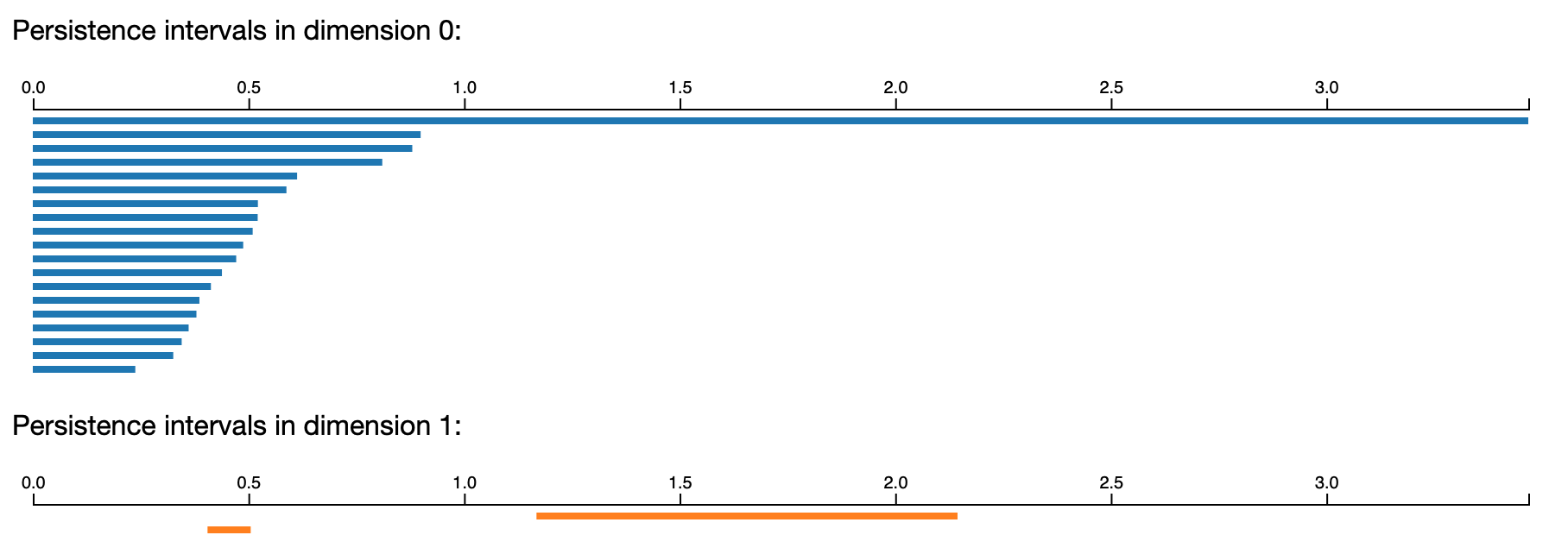
Figure 2. The barcode corresponding to the Vietoris–Rips complex in Figure 1. The image is generated by Ripser for Python.

Since $(X,d_{X})$ is a finite pseudo-metric space, it follows that $R(X,t)$ is contractible when $t$ is large enough. Therefore, the corresponding barcode $B(X)$ is a finite collection of half-open persistence intervals with finite lengths. If we use the unreduced simplicial homology in the definition of persistent homology, then the barcode would contain a single infinite interval $[0,\infty)$ in dimension $0$. Figure 2 displays the unreduced barcode corresponding to the Vietoris–Rips filtration in Figure 1.

3. Moment-angle complexes and bigraded Betti numbers

3.1. Cohomology of moment angle complexes

Let $K$ be a simplicial complex on the set $[m]=\{1,2,\ldots,m\}$. We refer to a subset $I=(i_{1},\ldots,i_{k})\subset[m]$ that is contained in $K$ as a simplex. A one-element simplex $\{i\}\in K$ is a vertex. We also assume that $\varnothing\in K$ and, unless explicitly stated otherwise, that $K$ contains all one-element subsets $\{i\}\in[m]$ (that is, $K$ is a simplicial complex without ghost vertices).

Let $D^{2}$ be the unit disc in $\mathbb{R}^{2}$, and let $S^{1}$ be its boundary circle. For each simplex $I\in K$, consider the topological space

$$(D^{2},S^{1})^{I}\colonequals\{(z_{1},\dots,z_{m})\in(D^{2})^{m}\colon|z_{j}|=1\text{ if }j\notin I\}\subset(D^{2})^{m}.$$

Note that $(D^{2},S^{1})^{I}$ is a natural subspace of $(D^{2},S^{1})^{J}$ whenever $I\subset J$. The moment-angle complex corresponding to $K$ is

$$\mathcal{Z}_{K}\colonequals\bigcup_{I\in K}(D^{2},S^{1})^{I}\subset(D^{2})^{m}.$$

We refer to [BP, Chapter 4] for more details and examples.

Let $\mathbf{k}$ be a coefficient ring, which we assume to be a principal ideal domain. The face ring (the Stanley–Reisner ring) of a simplicial complex $K$ is

$$\mathbf{k}[K]\colonequals\mathbf{k}[v_{1},\dots,v_{m}]/\mathcal{I}_{K},$$

where $\mathcal{I}_{K}$ is the ideal generated by square-free monomials $\prod_{i\in I}v_{i}$ for which $I\subset[m]$ is not a simplex of $K$.

The following theorem summarizes several presentations of the cohomology ring $H^{\ast}(\mathcal{Z}_{K})$.

Theorem 3.1 ([BP, Section 4.5]).

There are isomorphisms of bigraded commutative algebras

$$H^{*}(\mathcal{Z}_{K}) \cong\mathop{\mathrm{Tor}}\nolimits_{\mathbf{k}[v_{1},\ldots,v_{m}]}\bigl{(}\mathbf{k},\mathbf{k}[K]\bigr{)}$$

(3.1) $$\cong H\bigl{(}\Lambda[u_{1},\ldots,u_{m}]\otimes\mathbf{k}[K],d\bigr{)}$$

(3.2) $$\cong\bigoplus_{I\subset[m]}\widetilde{H}^{*}(K_{I}).$$

Here, (3.1) is cohomology of the bigraded algebra with bidegrees $\mathop{\mathrm{bideg}}u_{i}=(-1,2)$, $\mathop{\mathrm{bideg}}v_{i}=(0,2)$ and differential $d=\sum_{i=1}^{m}v_{i}\frac{\partial}{\partial u_{i}}$ of bidegree $(1,0)$ (the Koszul complex). In (3.2), each component $\widetilde{H}^{*}(K_{I})$ denotes the reduced simplicial cohomology of the full subcomplex $K_{I}\subset K$ (the restriction of $K$ to $I\subset[m]$). The last isomorphism is the sum of isomorphisms

$$H^{p}(\mathcal{Z}_{K})\cong\sum_{I\subset[m]}\widetilde{H}^{p-|I|-1}(K_{I}),$$

and the ring structure is given by the maps

$$H^{p-|I|-1}(K_{I})\otimes H^{q-|J|-1}(K_{J})\to H^{p+q-|I|-|J|-1}(K_{I\cup J})$$

which are induced by the canonical simplicial maps $K_{I\cup J}\to K_{I}\mathbin{*}K_{J}$ for $I\cap J=\varnothing$ and zero otherwise.

Isomorphism (3.2) is often referred to as the Hochster decomposition, as it comes from Hochster’s theorem describing $\mathop{\mathrm{Tor}}\nolimits_{\mathbf{k}[v_{1},\ldots,v_{m}]}(\mathbf{k},\mathbf{k}[K])$ as a sum of cohomology of full subcomplexes $K_{I}$.

The bigraded components of cohomology of $\mathcal{Z}_{K}$ are given by

$$H^{-i,2j}(\mathcal{Z}_{K})\cong H^{-i,2j}\bigl{(}\Lambda[u_{1},\ldots,u_{m}]\otimes\mathbf{k}[K],d\bigr{)}\cong\bigoplus_{J\subset[m]\colon|J|=j}\widetilde{H}^{j-i-1}(K_{J}),\quad$$

so that

$$H^{p}(\mathcal{Z}_{K})=\bigoplus_{-i+2j=p}H^{-i,2j}(\mathcal{Z}_{K})\cong\bigoplus_{J\subset[m]}\widetilde{H}^{p-|J|-1}(K_{J}),$$

There is a similar description of bigraded homology of $\mathcal{Z}_{K}$:

$$H_{p}(\mathcal{Z}_{K})=\bigoplus_{-i+2j=p}H_{-i,2j}(\mathcal{Z}_{K})\cong\bigoplus_{J\subset[m]}\widetilde{H}_{p-|J|-1}(K_{J}).$$

The construction of moment-angle complex and its bigraded homology is functorial with respect to inclusion of simplicial complexes:

Proposition 3.2.

An inclusion of subcomplex $K\subset L$ induces an inclusion $\mathcal{Z}_{K}\subset\mathcal{Z}_{L}$ and a homomorphism $H_{-i,2j}(\mathcal{Z}_{K})\to H_{-i,2j}(\mathcal{Z}_{L})$ of bigraded homology modules.

When $\mathbf{k}$ is a field, the bigraded Betti numbers of $K$ (with coefficients in $\mathbf{k}$) are defined by

$$\beta_{-i,2j}(K)\colonequals\dim H_{-i,2j}(\mathcal{Z}_{K})=\sum_{J\subset[m]\colon|J|=j}\dim\widetilde{H}_{j-i-1}(K_{J}).$$

In particular, when $j=m$, we obtain $\beta_{-i,2m}(K)=\dim\widetilde{H}_{m-i-1}(K)$. Moreover, $\dim\widetilde{H}^{j-i-1}(K_{J})$ agrees with $\dim\widetilde{H}_{j-i-1}(K_{J})$ obviously.

Dimensional considerations imply that possible locations of nonzero bigraded Betti numbers form a trapezoid in the table, see Figure 3. We refer to [BP, Section 4.5] for more details.

Figure 3. Table of bigraded Betti numbers.

3.2. Bigraded persistence and barcodes

Definition 3.3.

Let $(X,d_{X})$ be a finite pseudo-metric space and $(X,d_{X})$ and $\{R(X,t)\}_{t\geq 0}$ its associated Vietoris–Rips filtration. We define the bigraded persistent homology module of bidegree $(-i,2j)$ as

$$\mathcal{PHZ}_{-i,2j}(X)\colon{\mathbb{R}}_{\geq 0}\to\mathbf{k}\textsc{-mod},\quad t\mapsto H_{-i,2j}(\mathcal{Z}_{R(X,t)}).$$

It maps $t\in{\mathbb{R}}_{\geq 0}$ to the bigraded homology module $H_{-i,2j}(\mathcal{Z}_{R(X,t)})$ and maps a morphism $t_{1}\leq t_{2}$ to the homomorphism $H_{-i,2j}(\mathcal{Z}_{R(X,t_{1})})\to H_{-i,2j}(\mathcal{Z}_{R(X,t_{2})})$, see Proposition 3.2. We also define the bigraded persistent homology module

(3.3) $$\mathcal{PHZ}(X)=\bigoplus_{\begin{subarray}{c}0\leq i\leq m-1;\\ 0\leq j\leq m\end{subarray}}\mathcal{PHZ}_{-i,2j}(X).$$

For any subset $J\subset X$, the Vietoris–Rips complex $R(J,t)$ is the full subcomplex $R(X,t)_{J}$. Hence, the Hochster decomposition (3.2) yields the decomposition of the persistence modules:

(3.4) $$\mathcal{PHZ}(X)=\bigoplus_{J\subset X}\mathcal{PH}(J).$$

The bigraded barcode $\mathit{BB}(X)$ is the collection of persistence intervals of generators of the bigraded homology groups $H_{-i,2j}(\mathcal{Z}_{R(X,t)})$. We note that bigraded persistence intervals are defined in the same way as for ordinary persistent homology, see Subsection 2.2. For each $t\in\mathbb{R}_{\geq 0}$, the dimension of $H_{-i,2j}(\mathcal{Z}_{R(X,t)})$ is equal to the number of persistence intervals of bidegree $(-i,2j)$ containing $t$.

The bigraded barcode of $X$ is drawn as a diagram in $3$-dimensional space, which contains the original barcode of $X$ in its top level. See Figure 4.

Figure 4. A bigraded barcode.

Here is a simple example of two sequences of point clouds with the same barcodes, but different bigraded barcodes.

Example 3.4.

Let $X_{1}$ and $X_{2}$ consist of three points $(0,0),(2,0),(0,4)$ and $(0,0),(2,0),(1,\sqrt{15})$ in ${\mathbb{R}}^{3}$, respectively. The Vietoris–Rips filtration $\{R(X_{1},t)\}_{t\geq 0}$ at $t=0,2,4,2\sqrt{5}$ is shown in Figure 5, top, and the Vietoris–Rips filtration $\{R(X_{2},t)\}_{t\geq 0}$ at $t=0,2,4$ is shown in Figure 5, bottom. The corresponding bigraded barcodes are shown in Figure 6. We notice that the two bars in the top levels of the bigraded barcodes are identical. These two bars represent the ordinary (single graded) barcodes of $X_{1}$ and $X_{2}$, respectively. The two data sets $X_{1}$ and $X_{2}$ are distinguished by their bigraded barcodes.

Figure 5. Two sequences of Vietoris–Rips complexes.

Figure 6. The bigraded barcode for 3 points in ${\mathbb{R}}^{2}$.

3.3. Double cohomology of moment angle complexes

In [LPSS], the homology of the moment-angle complex $H_{*}(\mathcal{Z}_{K})=\bigoplus_{I\subset[m]}\widetilde{H}_{*}(K_{I})$ was endowed with the second differential $\partial^{\prime}$. The homology of the resulting chain complex $\mathit{CH}_{*}(\mathcal{Z}_{K})=(H_{*}(\mathcal{Z}_{K}),\partial^{\prime})$ was called the double homology of $\mathcal{Z}_{K}$. We use this construction to define a new bigraded persistence module $\mathcal{PHHZ}(X)$.

Given $j\in[m]\setminus I$, consider the homomorphism

$$\phi_{p;I,j}\colon\widetilde{H}_{p}(K_{I})\to\widetilde{H}_{p}(K_{I\sqcup\{j\}})$$

induced by the inclusion $K_{I}\hookrightarrow K_{I\cup\{j\}}$. Then define

$$\partial^{\prime}_{p}=(-1)^{p+1}\bigoplus_{I\subset[m],\,j\in[m]\setminus I}\varepsilon(j,I)\,\phi_{p;I,j},$$

where

$$\varepsilon(j,I)=(-1)^{\#\{i\in I\colon i<j\}}.$$

The homomorphism $\partial^{\prime}_{p}\colon\bigoplus_{I\subset[m]}\widetilde{H}_{p}(K_{I})\to\bigoplus_{I\subset[m]}\widetilde{H}_{p}(K_{I})$ satisfies $(\partial^{\prime}_{p})^{2}=0$. We therefore have a chain complex

(3.5) $$\mathit{CH}_{\ast}(\mathcal{Z}_{K})\colonequals(H_{\ast}(\mathcal{Z}_{K}),\partial^{\prime}),\quad\partial^{\prime}\colon\widetilde{H}_{-i,2j}(\mathcal{Z}_{K})\to\widetilde{H}_{-i-1,2j+2}(\mathcal{Z}_{K}),$$

and bigraded double homology of $\mathcal{Z}_{K}$:

$$\mathit{HH}_{\ast}(\mathcal{Z}_{K})=H(H_{\ast}(\mathcal{Z}_{K}),\partial^{\prime}).$$

Double cohomology of $\mathcal{Z}_{K}$ is defined similarly:

$$\mathit{HH}^{\ast}(\mathcal{Z}_{K})=H(H^{\ast}(\mathcal{Z}_{K}),d^{\prime}),\quad d^{\prime}\colon\widetilde{H}^{-i,2j}(\mathcal{Z}_{K})\to\widetilde{H}^{-i+1,2j-2}(\mathcal{Z}_{K})$$

Double cohomology $\mathit{HH}^{\ast}(\mathcal{Z}_{K})$ can also be defined as the first double cohomology of the bicomplex $\bigl{(}\Lambda[u_{1},\ldots,u_{m}]\otimes\mathbf{k}[K],d,d^{\prime}\bigr{)}$ with $d=\sum_{i=1}^{m}v_{i}\frac{\partial}{\partial u_{i}}$, $d^{\prime}=\sum_{i=1}^{m}\frac{\partial}{\partial u_{i}}$ and $dd^{\prime}=-d^{\prime}d$:

$$\mathit{HH}^{*}(\mathcal{Z}_{K})\cong H\bigl{(}H\bigl{(}\Lambda[u_{1},\ldots,u_{m}]\otimes\mathbf{k}[K],d\bigr{)},d^{\prime}\bigr{)},$$

see [LPSS, Theorem 4.3].

If $K=\Delta^{m-1}$, the full simplex on $[m]$, then double homology is trivial:

$$\mathit{HH}_{*}(\mathcal{Z}_{K})=\mathbf{k}_{(0,0)}$$

(the latter means that $\mathit{HH}_{0,0}(\mathcal{Z}_{K})\cong\mathbf{k}$ and $\mathit{HH}_{-i,2j}(\mathcal{Z}_{K})=0$ if $(-i,2j)\neq(0,0)$).

An important property of double homology is that attaching a simplex to $K$ along a face (in particular, adding a disjoint simplex) destroys most of $\mathit{HH}_{*}(\mathcal{Z}_{K})$, as described next:

Theorem 3.5 ([LPSS, Theorem 6.7]).

Let $K=K^{\prime}\cup_{I}\Delta^{n}$ be a simplicial complex obtained from a nonempty simplicial complex $K^{\prime}$ by gluing an $n$-simplex, $n\geq 0$, along a proper, possibly empty, face $I\in K$. Then either $K$ is a simplex, or

$$\mathit{HH}_{*}(\mathcal{Z}_{K})=\mathbf{k}_{(0,0)}\oplus\mathbf{k}_{(-1,4)}.$$

Definition 3.6.

Let $(X,d_{X})$ be a finite metric space. A point $x\in X$ is an outlier if for any $y\neq x$ holds the inequality

$$d_{X}(x,y)\geq\max_{y^{\prime}\neq x}d_{X}(y,y^{\prime}).$$

Proposition 3.7.

Suppose a finite metric space $(X,d_{X})$ has an outlier. Let $D$ be the diameter of $(X,d_{X})$, and let $R(X,t)$ be the Vietoris–Rips complex associated with $(X,d_{X})$. Then,

$$\mathit{HH}_{\ast}(\mathcal{Z}_{R(X,t)})=\begin{cases}\mathbf{k}_{(0,0)}&t\geq D;\\ \mathbf{k}_{(0,0)}\oplus\mathbf{k}_{(-1,4)}&t<D\end{cases}$$

with all maps $\mathit{HH}_{\ast}(\mathcal{Z}_{R(X,t)})\to\mathit{HH}_{\ast}(\mathcal{Z}_{R(X,t^{\prime})})$ being the identity if $D\leq t\leq t^{\prime}$, and the projection if $t<D\leq t^{\prime}$.

Proof.

The definition of an outlier $x$ implies that the Vietoris–Rips complex $R(X,t)$ is obtained from the Vietoris–Rips complex $R(X\setminus x,t)$ by attaching a simplex (with vertices $x$ and $\{y\colon d(x,y)\leq t\}$) along its facet (with vertices $\{y\colon d(x,y)\leq t\}$). For $t\geq D$, the complex $R(X,t)$ is a simplex itself. Then the result follows from Theorem 3.5. ∎

We define the bigraded persistent double homology and the corresponding barcodes by analogy with Definition 3.3:

Definition 3.8.

Let $(X,d_{X})$ be a finite pseudo-metric space and $\{R(X,t)\}_{t\geq 0}$ its associated Vietoris–Rips filtration. The bigraded persistent double homology module of bidegree $(-i,2j)$ is

$$\mathcal{PHHZ}_{-i,2j}(X)\colon{\mathbb{R}}_{\geq 0}\to\mathbf{k}\textsc{-mod},\quad t\mapsto\mathit{HH}_{-i,2j}(\mathcal{Z}_{R(X,t)}).$$

It maps $t\in{\mathbb{R}}_{\geq 0}$ to the bigraded module $\mathit{HH}_{-i,2j}(\mathcal{Z}_{R(X,t)})$ and maps a morphism $t_{1}\leq t_{2}$ to the homomorphism $\mathit{HH}_{-i,2j}(\mathcal{Z}_{R(X,t_{1})})\to\mathit{HH}_{-i,2j}(\mathcal{Z}_{R(X,t_{2})})$ induced by the inclusion $\mathcal{Z}_{R(X,t_{1})}\to\mathcal{Z}_{R(X,t_{2})}$ (see [LPSS, Proposition 4.8]). We also define the bigraded persistent homology module

(3.6) $$\mathcal{PHHZ}(X)=\bigoplus_{\begin{subarray}{c}0\leq i\leq m-1;\\ 0\leq j\leq m\end{subarray}}\mathcal{PHHZ}_{-i,2j}(X).$$

One can view the bigraded persistent homology module (3.3) as a functor to differential bigraded $\mathbf{k}$-modules,

$$\mathcal{PHZ}(X)\colon{\mathbb{R}}_{\geq 0}\to\textsc{dg}(\mathbf{k}\textsc{-mod}),\quad t\mapsto(H_{*,*}(\mathcal{Z}_{R(X,t)}),\partial^{\prime}).$$

Then we have

(3.7) $$\mathcal{PHHZ}(X)=\mathcal{H}\circ\mathcal{PHZ}(X),$$

where $\mathcal{H}\colon\textsc{dg}(\mathbf{k}\textsc{-mod})\to\mathbf{k}\textsc{-mod}$ is the homology functor. This will be convenient when we compare interleaving distances. We denote by $\mathbb{BB}(X)$ the barcode corresponding to the bigraded persistence module $\mathcal{PHHZ}(X)$.

Example 3.9.

Suppose $(X,d_{X})$ has an outlier. Then $\mathbb{BB}(X)$ consists of an infinite bar $[0,\infty)$ at bidegree $(0,0)$ and a bar $[0,D)$ at bidegree $(-1,4)$, by Proposition 3.7.

4. Stability

In this section, we establish stability properties of the bigraded persistence modules $\mathcal{PHZ}(X)$ and $\mathcal{PHHZ}(X)$, see Theorems 4.20 and 4.22.

4.1. Distance functions

We first summarize several distance functions defined on the categories of finite pseudo-metric spaces and persistence modules.

Definition 4.1.

The Hausdorff distance between two nonempty subsets $A$ and $B$ in a finite pseudo-metric space $(Z,d)$ is

$$d_{H}(A,B)\vcentcolon=\max\bigl{\{}\sup_{a\in A}d(a,B),\,\sup_{b\in B}d(A,b)\bigr{\}}.$$

The Gromov–Hausdorff distance between two finite pseudo-metric spaces $X$ and $Y$ is

$$\mathop{d_{\mathit{GH}}}(X,Y)\vcentcolon=\inf_{Z,f,g}d_{H}(f(X),g(Y)),$$

where the infimum is taken over all isometric embeddings $f\colon X\to Z$ and $g\colon Y\to Z$ into a pseudo-metric space $Z$.

Using the notion of a correspondence between two sets, one can give an alternative definition of the Gromov–Hausdorff distance, which is often convenient for computational purposes.

Definition 4.2.

Given two sets $X$ and $Y$ and a subset $C$ of $X\times Y$, define $D_{C}(x)$ as the number of $y\in Y$ for which $(x,y)\in C$. Similarly, define $D_{C}(y)$ as the number of $x\in X$ for which $(x,y)\in C$. A correspondence between two sets $X$ and $Y$ is a subset $C$ of $X\times Y$ such that both $D_{C}(x)$ and $D_{C}(y)$ are nonzero.

Note that the condition $D_{C}(x)\geq 1$ for all $x\in C$ is equivalent to saying that $C$ is a (multi-valued) mapping with domain $X$ and range $Y$. Furthermore, the condition $D_{C}(y)\geq 1$ is equivalent to saying that $C$ is surjective.

Proposition 4.3 ([BBI, Theorem 7.3.25]).

For two finite pseudo-metric spaces $(X,d_{X})$ and $(Y,d_{Y})$,

(4.1) $$\mathop{d_{\mathit{GH}}}(X,Y)=\frac{1}{2}\min\limits_{C}\max\limits_{(x_{1},y_{1}),(x_{2},y_{2})\in C}|d_{X}(x_{1},x_{2})-d_{Y}(y_{1},y_{2})|.$$

We have the following modification of the Gromov–Hausdorff distance (4.1), to be used below.

Definition 4.4.

For two finite pseudo-metric spaces $(X,d_{X})$ and $(Y,d_{Y})$ of the same cardinality, define $\mathop{d^{\prime}_{\mathit{GH}}}(X,Y)$ by formula (4.1) in which the infimum is taken over bijective correspondences $C$ only.

Obviously, $\mathop{d^{\prime}_{\mathit{GH}}}(X,Y)\geq\mathop{d_{\mathit{GH}}}(X,Y)$ for any pair of pseudo-metric spaces of the same cardinality. The next example shows that for two pseudo-metric spaces $X$ and $Y$ of the same cardinality, the difference between $\mathop{d_{\mathit{GH}}}(X,Y)$ and $\mathop{d^{\prime}_{\mathit{GH}}}(X,Y)$ can be arbitrary large.

Example 4.5.

Fix $n>2$. Let $X$ consist of four vertices of a rectangle in $\mathbb{R}^{2}$ with two edges of length $1$ and diagonals of length $n$. Let $Y$ consist of four vertices of a tetrahedron in $\mathbb{R}^{3}$ with the base an equilateral triangle with edges of length 1 and the other three edges of length $n$. See Figure 7. It is easy to see that $\mathop{d^{\prime}_{\mathit{GH}}}(X,Y)=\frac{1}{2}(n-1)$, while $\mathop{d_{\mathit{GH}}}(X,Y)=\frac{1}{2}$.

Figure 7. Pseudo-metric spaces $X$ and $Y$ with $d_{GH}(X,Y)\neq d^{\prime}_{GH}(X,Y).$

Next, we introduce a distance function for persistence modules.

Given a persistence module $\mathcal{M}$ as in (2.1) and an arbitrary $\epsilon\in{\mathbb{R}}_{\geq 0}$, we define

$$\mathcal{M}^{\epsilon}\colon{\mathbb{R}}_{\geq 0}\to\mathbf{k}\textsc{-mod}$$

by $\mathcal{M}^{\epsilon}(s)=\mathcal{M}(s+\epsilon)$ and $\mathcal{M}^{\epsilon}(\phi_{s_{1},s_{2}})=\phi_{s_{1}+\epsilon,s_{2}+\epsilon}$. There is a natural transformation

$$\eta^{\epsilon}_{\mathcal{M}}\colon\mathcal{M}\to\mathcal{M}^{\epsilon}$$

defined by the family of morphisms $\{M_{s}\to M_{s+\epsilon}\mid s\in\mathbb{R}_{\geq 0}\}$.

Given two persistence modules $\mathcal{M}$ and $\mathcal{N}$, we say that $\mathcal{M}$ and $\mathcal{N}$ are $\epsilon$-interleaved if there exist natural transformations

$$\beta\colon\mathcal{M}\to\mathcal{N}^{\epsilon}\quad\text{ and }\quad\gamma\colon\mathcal{N}\to\mathcal{M}^{\epsilon}$$

such that $\beta^{\epsilon}\circ\gamma=\eta_{\mathcal{N}}^{2\epsilon}$ and $\gamma^{\epsilon}\circ\beta=\eta_{\mathcal{M}}^{2\epsilon}$, where $\beta^{\epsilon}\colon\mathcal{M}^{\epsilon}\to\mathcal{N}^{2\epsilon}$ and $\gamma^{\epsilon}\colon\mathcal{N}^{\epsilon}\to\mathcal{M}^{2\epsilon}$ denote the $\epsilon$-shifts of $\beta$ and $\gamma$, respectively.

Definition 4.6.

The interleaving distance between two persistence modules $\mathcal{M}$ and $\mathcal{N}$ is

$$d_{\mathit{IL}}(\mathcal{M},\mathcal{N})\colonequals\inf\{\epsilon\in{\mathbb{R}}_{\geq 0}\mid\mathcal{M}\text{ and }\mathcal{N}\text{ are $\epsilon$-interleaved}\}.$$

Example 4.7.

The interleaving distance between two interval modules $\mathbf{k}\left([a,b)\right)$ and $\mathbf{k}\left([a^{\prime},b^{\prime})\right)$ (see Example 2.1) is given by

$$d_{\mathit{IL}}\big{(}\mathbf{k}\left([a,b)\right),\mathbf{k}\left([a^{\prime},b^{\prime})\right)\big{)}=\min\left\{\max\left\{\frac{b-a}{2},\frac{b^{\prime}-a^{\prime}}{2}\right\},\max\{|a^{\prime}-a|,|b^{\prime}-b|\}\right\}.$$

This formula has the following meaning. If the intervals are close to each other (the closure of each interval contains the midpoint of the other), then the distance is the maximum of the distances between their endpoints, i. e. $\max\{|a^{\prime}-a|,|b^{\prime}-b|\}$, which is the standard $l^{\infty}$-distance between the two intervals. If the intervals are far apart, then the distance is $\max\left\{\frac{b-a}{2},\frac{b^{\prime}-a^{\prime}}{2}\right\}$, where $\frac{b-a}{2}$ is the $l^{\infty}$-distance between $[a,b)$ and a ‘zero length interval’ at the midpoint of $[a,b)$.

The zero persistence module can be thought of as the interval module $\mathbf{k}(\varnothing)$ of an empty interval. In this case, the interleaving distance is given by

$$d_{\mathit{IL}}\big{(}\mathbf{k}\left([a,b)\right),\mathbf{k}(\varnothing)\big{)}=\frac{b-a}{2}.$$

Below, we record the following properties of $d_{\mathit{IL}}$ for future use.

Proposition 4.8 (see [CS, Proposition 5.5]).

Let $\mathcal{M}_{1}$, $\mathcal{M}_{2}$, $\mathcal{N}_{1}$ and $\mathcal{N}_{2}$ be persistence modules. Then

$$d_{\mathit{IL}}(\mathcal{M}_{1}\oplus\mathcal{M}_{2},\mathcal{N}_{1}\oplus\mathcal{N}_{2})\leq\max\bigl{(}d_{\mathit{IL}}(\mathcal{M}_{1},\mathcal{N}_{1}),d_{\mathit{IL}}(\mathcal{M}_{2},\mathcal{N}_{2})\bigr{)}.$$

More generally, the interleaving distance can be defined for persistence modules $\mathcal{M}\colon{\mathbb{R}}_{\geq 0}\to\textsc{c}$ taking values in any Grothendieck category c instead of $\mathbf{k}\textsc{-mod}$, see [BSS]. The following result is clear from the definition.

Proposition 4.9.

Given two functors $\mathcal{M}$ and $\mathcal{N}$ from ${\mathbb{R}}_{\geq 0}$ to c, and a functor $\mathcal{F}\colon\textsc{c}\to\textsc{d}$, we have:

$$d_{\mathit{IL}}(\mathcal{F}\circ\mathcal{M},\mathcal{F}\circ\mathcal{N})\leq d_{\mathit{IL}}(\mathcal{M},\mathcal{N}).$$

Next, we introduce the bottleneck distance between multisets of intervals (or barcodes). It is defined in the standard way as the infimum over matchings between them, in which some of the intervals can be matched to zero length intervals at their midpoints.

Let $B$ and $B^{\prime}$ be finite multisets of intervals of the form $[a,b)$ with $a\in{\mathbb{R}}_{\geq 0}$ and $b\in{\mathbb{R}}_{\geq 0}\cup\{\infty\}$. Define the multiset $\overline{B}=B\cup\varnothing^{|B^{\prime}|}$, obtained by adding to $B$ the multiset containing the empty interval $\varnothing$ with cardinality $|B^{\prime}|$. Similarly, define $\overline{B^{\prime}}=B^{\prime}\cup\varnothing^{|B|}$. Note that $\overline{B}$ and $\overline{B^{\prime}}$ have the same cardinality. We define the distance function

$$\pi\colon\overline{B}\times\overline{B^{\prime}}\to{\mathbb{R}}_{\geq 0}\cup\{\infty\}$$

by the formulae:

$$\pi\left([a,b),[a^{\prime},b^{\prime})\right)=\max\{|a^{\prime}-a|,|b^{\prime}-b|\},\quad\pi([a,\infty),[a^{\prime},\infty))=|a^{\prime}-a|,$$

$$\pi([a,b),\varnothing)=\frac{b-a}{2},\quad\pi(\varnothing,[a^{\prime},b^{\prime}))=\frac{b^{\prime}-a^{\prime}}{2},\quad\pi(\varnothing,\varnothing)=0,$$

$$\pi([a,\infty),[a^{\prime},b^{\prime}))=\pi([a,b),[a^{\prime},\infty))=\pi([a,\infty),\varnothing)=\pi(\varnothing,[a^{\prime},\infty))=\infty$$

for finite $a,b,a^{\prime},b^{\prime}$.

Definition 4.10.

Denote by $\mathcal{D}\left(\overline{B},\overline{B^{\prime}}\right)$ the set of all bijections $\theta\colon\overline{B}\to\overline{B^{\prime}}$. Then the $\infty$-Wasserstein distance, also called the bottleneck distance, is defined as follows:

$$W_{\infty}(B,B^{\prime})=\min_{\theta\in\mathcal{D}(\overline{B},\overline{B^{\prime}})}\max_{I\in\overline{B}}\,\pi(I,\theta(I)).$$

It can be shown [BS, Definition 4.11] that

$$W_{\infty}(B,B^{\prime})=\min_{\theta\in\mathcal{D}(\overline{B},\overline{B^{\prime}})}\max_{I\in\overline{B}}\,d_{\mathit{IL}}\bigl{(}\mathbf{k}(I),\mathbf{k}(\theta(I))\bigr{)},$$

where the interleaving distance between interval modules can be expressed via the $l^{\infty}$-distance as in Example 4.7.

Example 4.11.

1. Let $B=\{[0,5)\}$ and $B^{\prime}=\{[1,7)\}$. Then $\overline{B}=\{[0,5),\varnothing\}$ and $\overline{B^{\prime}}=\{[1,7),\varnothing\}$. There are two bijections between $\overline{B}$ and $\overline{B^{\prime}}$:

$$\theta_{1}\colon[0,5)\mapsto[1,7),\,\varnothing\mapsto\varnothing,\quad\text{and}\quad\theta_{2}\colon[0,5)\mapsto\varnothing,\,\varnothing\mapsto[1,7).$$

The minimum of $\max_{I\in\overline{B}}\,\pi(I,\theta(I))$ is achieved at $\theta_{1}$, which reflects the fact that the two intervals overlap sufficiently. We have $W_{\infty}(B,B^{\prime})=\pi([0,5),[1,7))=7-5=2$.

2. Let $B=\{[0,5)\}$ and $B^{\prime}=\{[3,9)\}$. These two intervals are ‘far apart’, so the minimum of $\max_{I\in\overline{B}}\,\pi(I,\theta(I))$ is achieved when both $[0,5)$ and $[3,9)$ are matched to an empty interval. We have $W_{\infty}(B,B^{\prime})=\pi(\varnothing,[3,9))=3$.

In the literature, the following result is often referred to as the isometry theorem, see [Le, Theorem 3.4]. We also refer to [BS, Theorem 4.16] and [CS, Theorem 5.14] for different versions of this result:

Theorem 4.12.

Let $\mathcal{M}$ and $\mathcal{N}$ be persistence modules satisfying the hypothesis of Theorem 2.2. Then,

$$d_{\mathit{IL}}(\mathcal{M},\mathcal{N})=W_{\infty}(B(\mathcal{M}),B(\mathcal{N})),$$

where $B(\mathcal{M})$ and $B(\mathcal{N})$ are the barcodes corresponding to $\mathcal{M}$ and $\mathcal{N}$, respectively.

The stability theorem asserts that the persistent homology barcodes are stable under perturbations of the data sets in the Gromov–Hausdorff metric. It is a key result justifying the use of persistent homology in data science. We refer to [CC, Theorem 3.1] and [CDO, Lemma 4.3, Theorem 5.2] for the proof:

Theorem 4.13.

Let $(X,d_{X})$ and $(Y,d_{Y})$ be two finite pseudo-metric spaces, and let $B(X)$ and $B(Y)$ be the barcodes corresponding to the persistence modules $\mathcal{PH}(X)$ and $\mathcal{PH}(Y)$. Then,

$$d_{\mathit{IL}}(\mathcal{PH}(X),\mathcal{PH}(Y))\leq 2d_{GH}(X,Y),$$

and when working over a field,

$$W_{\infty}(B(X),B(Y))\leq 2d_{GH}(X,Y).$$

4.2. The doubling operation

The following construction plays a key role in proving the stability property of persistent double homology.

Definition 4.14.

Given a pseudo-metric space $(X,d_{X})$ and a point $x\in X$, we refer to the pseudo-metric space $X^{\prime}=X\sqcup\{x^{\prime}\}$ with $d_{X^{\prime}}(x,x^{\prime})=0$ as the doubling of $X$ at $x$.

Given a simplicial complex $K$ on $[m]$ and a vertex $\{i\}$ of $K$, the doubling of $K$ at $\{i\}$ is the minimal simplicial complex $K^{\prime}$ on the set $[m]\sqcup\{i^{\prime}\}$ which contains $K$ and all subsets $I\sqcup\{i^{\prime}\}$, where $i\in I\in K$. There is a deformation retraction $K^{\prime}\to K$ sending $\{i^{\prime}\}$ to $\{i\}$ and identity on other vertices. See Figure 8.

Figure 8. Doubling at a vertex.

The doubling at a vertex is a particular case of the following operation introduced in [AP]. Let $K$ be a simplicial complex on the set $[m]$, and let $K_{1},\ldots,K_{m}$ be simplicial complexes. The substitution of $K_{1},\ldots,K_{m}$ into $K$ is the simplicial complex

$$K(K_{1},\ldots,K_{m})=\{I_{j_{1}}\sqcup\dots\sqcup I_{j_{k}}\colon I_{j_{l}}\in K_{j_{l}},\;l=1,\dots,k\quad\text{and}\quad\{j_{1},\dots,j_{k}\}\in K\}.$$

The doubling of $K$ at $\{i\}$ is the substitution complex $K(1,\ldots,\Delta[i,i^{\prime}],\ldots,m)$, where $\Delta[i,i^{\prime}]$ denotes the 1-simplex on $i$ and $i^{\prime}$.

Observe that if $X^{\prime}$ is the doubling of a pseudo-metric space $X$ at a point, then the Vietoris–Rips complex $R(X^{\prime},t)$ is the doubling of $R(X,t)$ at a vertex, i. e. $R(X^{\prime},t)=R(X,t)^{\prime}$.

Proposition 4.15.

Suppose $\widehat{X}$ is obtained from $X$ by an arbitrary number of doubling operations performed at arbitrary points on the way. Then $d_{GH}(X,\widehat{X})=0$.

Proof.

Using the triangle inequality, we reduce the claim to the case when $\widehat{X}$ is obtained from $X$ by a single doubling operation, i. e. $\widehat{X}=X^{\prime}=X\sqcup\{x_{0}^{\prime}\}$ is a doubling at $x_{0}\in X$.

We use (4.1) and consider the following correspondence $C$ between $X$ and $X^{\prime}$:

$$C\colonequals\{(x,x)\in X\times X^{\prime}\mid x\in X\}\sqcup\{(x_{0},x_{0}^{\prime})\}.$$

Note that for any $s\in X$ with $s\neq x_{0}$, the number $D_{C}(s)$ of $x\in X^{\prime}$ for which $(s,x)\in C$ is $1$. Similarly, $D_{C}(x_{0})=2$ and $D_{C}(t)=1$ for all $t\in X^{\prime}$. See Definition 4.2. The triangle inequality together with $d_{X^{\prime}}(x_{0},x_{0}^{\prime})=0$ implies $d_{X}(x_{1},x_{2})=d_{X^{\prime}}(y_{1},y_{2})$ for any $(x_{1},y_{1}),(x_{2},y_{2})\in C$, hence $d_{GH}(X,X^{\prime})=0$. ∎

Proposition 4.16.

Given two finite pseudo-metric spaces $X$ and $Y$, there exist two finite pseudo-metric spaces $\widehat{X}$ and $\widehat{Y}$ such that $|\widehat{X}|=|\widehat{Y}|$ and

$$d_{GH}(X,Y)=d^{\prime}_{GH}(\widehat{X},\widehat{Y}),$$

where $d_{GH}^{\prime}$ is the modified Gromov–Hausdorff distance, see Definition 4.4.

Proof.

For two finite pseudo-metric spaces $S$ and $T$ of the same cardinality, we have

(4.2) $$d_{GH}(S,T)\leq d^{\prime}_{GH}(S,T),$$

because any bijection is a correspondence between $S$ and $T$.

Now let $\widehat{X}$ and $\widehat{Y}$ be pseudo-metric spaces obtained by iterated doublings of $X$ and $Y$, respectively, so that $\widehat{X}$ and $\widehat{Y}$ have the same cardinality. The triangle inequality together with Proposition 4.15 implies

$$\begin{split}d_{GH}(X,Y)&\leq d_{GH}(X,\widehat{X})+d_{GH}(\widehat{X},\widehat{Y})+d_{GH}(\widehat{Y},Y)\\ &=d_{GH}(\widehat{X},\widehat{Y})\leq d^{\prime}_{GH}(\widehat{X},\widehat{Y}),\end{split}$$

where second equality follows from Proposition 4.15 and the last inequality follows from (4.2).

To complete the proof, we construct iterated doublings $\widehat{X}$ and $\widehat{Y}$ such that $d^{\prime}_{GH}(\widehat{X},\widehat{Y})\leq d_{GH}(X,Y)$. Let $C$ be a correspondence which realizes $d_{GH}(X,Y)$. If $C$ is a bijection (in particular, $|X|=|Y|$), then there is nothing to prove. So we assume that $C$ is not a bijection.

First, consider all the vertices $x\in X$ such that $D_{C}(x)>1$ and double each of them $D_{C}(x)-1$ times. We get a new pseudo-metric space $\widehat{X}$ and a new correspondence $C^{\prime}$ between $\widehat{X}$ and $Y$ which matches each double of $x$ with a single point of $Y$. If $C^{\prime}$ is a bijection, we set $\widehat{Y}=Y$ and we have

(4.3) $$\begin{split}d_{GH}(X,Y)&=\frac{1}{2}\max_{(x,y),(x^{\prime},y^{\prime})\in C}|d_{X}(x,x^{\prime})-d_{Y}(y,y^{\prime})|\\ &=\frac{1}{2}\max_{(x,y),(x^{\prime},y^{\prime})\in C^{\prime}}|d_{\widehat{X}}(x,x^{\prime})-d_{\widehat{Y}}(y,y^{\prime})|\geq d^{\prime}_{GH}(\widehat{X},\widehat{Y}),\end{split}$$

where the second equality follows because the set $\{|d_{X}(x,x^{\prime})-d_{Y}(y,y^{\prime})|\}_{(x,y),(x^{\prime},y^{\prime})\in C}$ coincides with $\{|d_{\widehat{X}}(x,x^{\prime})-d_{\widehat{Y}}(y,y^{\prime})\}_{(x,y),(x^{\prime},y^{\prime})\in C^{\prime}}$ and the last inequality follows from Definition 4.4.

If $C^{\prime}$ is not a bijection, then it is a single-valued surjective mapping from $\widehat{X}$ to $Y$, which is not yet injective, so we perform the next step. Consider all the vertices $y\in Y$ such that $D_{C^{\prime}}(y)>1$ and double each of them $D_{C^{\prime}}(y)-1$ times. We get a new pseudo-metric space $\widehat{Y}$ and a new correspondence $\widehat{C}$ between $\widehat{X}$ and $\widehat{Y}$ which matches each double of $y$ with a single point of $\widehat{X}$. Now, $\widehat{C}$ is an injective mapping from $\widehat{X}$ to $\widehat{Y}$, therefore it is a bijection. See Figure 9 for an example of this procedure. Now the same argument as in (4.3) establishes the claim.

Figure 9. From a correspondence to a bijection via iterated doublings.

∎

The proof of the last proposition also gives the following proposition. This could be helpful in proving other stability results.

Proposition 4.17.

Any correspondence between finite sets can be written as a composition of doublings and a single bijection.

Next we show that the doubling of simplicial complexes preserves the double homology of the corresponding moment-angle complexes.

Proposition 4.18.

Let $K^{\prime}$ be obtained from $K$ by doubling a vertex. Then,

$$\mathit{HH}_{\ast}(\mathcal{Z}_{K})\cong\mathit{HH}_{\ast}(\mathcal{Z}_{K^{\prime}}).$$

Proof.

Let $K^{\prime}$ be obtained by doubling of $K$ at $i\in[m]$. We recall the chain complex (3.5) and define the chain map

$$\varphi\colon\mathit{CH}_{\ast}(\mathcal{Z}_{K^{\prime}})=\Bigl{(}\bigoplus_{I\subset[m]\sqcup\{i^{\prime}\}}\widetilde{H}_{\ast}(K^{\prime}_{I}),\partial^{\prime}\Bigr{)}\to\mathit{CH}_{\ast}(\mathcal{Z}_{K})=\Bigl{(}\bigoplus_{J\subset[m]}\widetilde{H}_{\ast}(K_{J}),\partial^{\prime}\Bigr{)}$$

by the property that for $\alpha\in\widetilde{H}_{\ast}(K^{\prime}_{I})$,

$$\varphi(\alpha)=\begin{cases}0&\text{if }i^{\prime}\in I;\\ \alpha&\text{if }i^{\prime}\notin I.\end{cases}$$

We claim that the chain map $\varphi$ defined above is a weak equivalence. Since $\varphi$ is surjective, it suffices to show that $\ker\varphi$ is acyclic. Observe that

$$\ker\varphi\cong\bigoplus_{i^{\prime}\in I\subset[m]\sqcup\{i^{\prime}\}}\widetilde{H}_{\ast}\left(K^{\prime}_{I}\right)=\bigoplus_{L\subset[m]}\widetilde{H}_{*}(K^{\prime}_{L\sqcup\{i^{\prime}\}}).$$

Let $T_{n}\colonequals\{L\subset[m]\colon|L\setminus\{i\}|\geq n\}$ and define a decreasing filtration

$$\ker\varphi=F_{0}\supset F_{1}\supset\cdots\supset F_{n}\supset\cdots$$

with

$$F_{n}=\bigoplus_{L\in T_{n}}\widetilde{H}_{*}(K^{\prime}_{L\sqcup\{i^{\prime}\}}),\quad F_{n}/F_{n+1}=\bigoplus_{L\subset[m]\colon|L\setminus\{i\}|=n}\widetilde{H}_{*}(K^{\prime}_{L\sqcup\{i^{\prime}\}}).$$

The associated spectral sequence has $E^{0}_{n}=(F_{n}/F_{n+1},\overline{\partial^{\prime}})$, where the differential $\overline{\partial^{\prime}}$ induced by $\partial^{\prime}$, decomposes as a direct sum

$$\bigoplus_{i\notin L,\,|L|=n}\Bigl{(}\widetilde{H}_{\ast}(K^{\prime}_{L\sqcup\{i^{\prime}\}})\to\widetilde{H}_{\ast}(K^{\prime}_{L\sqcup\{i,i^{\prime}\}})\Bigr{)}.$$

Each map in the parentheses above is an isomorphism, because $K^{\prime}_{L\sqcup\{i^{\prime}\}}\subset K^{\prime}_{L\sqcup\{i,i^{\prime}\}}$ is a homotopy equivalence. Hence, the $E_{1}$-page of the spectral sequence is zero, so $\ker\varphi$ is acyclic. ∎

Proposition 4.19.

Suppose $\widehat{X}$ is a pseudo-metric space obtained from $X$ by an arbitrary number of doubling operations performed at arbitrary points. Then the persistent double homology modules $\mathcal{PHHZ}(X)$ and $\mathcal{PHHZ}(\widehat{X})$ are isomorphic.

Proof.

This follows from Proposition 4.18 and obvious functorial properties of the doubling construction. ∎

4.3. Stability for $\mathcal{PHZ}$

First, we establish a stability result for the bigraded persistence module $\mathcal{PHZ}(X)$ of a finite pseudo-metric space $(X,d_{X})$, see Definition 3.3.

Theorem 4.20.

For two finite pseudo-metric spaces $(X,d_{X})$ and $(Y,d_{Y})$ of the same cardinality, we have

$$d_{\mathit{IL}}(\mathcal{PHZ}(X),\mathcal{PHZ}(Y))\leq 2d_{GH}^{\prime}(X,Y),$$

where $d^{\prime}_{GH}$ is the modified Gromov–Hausdorff distance, see Definition 4.4.

Proof.

Let $\theta\colon X\to Y$ be the bijection that realizes $d^{\prime}_{GH}(X,Y)$. Then, for arbitrary subset $J\subset X$, we have

(4.4) $$d^{\prime}_{GH}(J,\theta(J))\leq d^{\prime}_{GH}(X,Y).$$

Let $\mathcal{PH}(J)$ and $\mathcal{PH}{(\theta(J))}$ be the ordinary persistent homology modules (2.4) corresponding to the subspaces $J$ and $\theta(J)$, respectively. Then,

(4.5) $$d_{\mathit{IL}}\bigl{(}\mathcal{PH}(J),\mathcal{PH}(\theta(J))\bigl{)}\leq 2d_{GH}(J,\theta(J))\leq 2d^{\prime}_{GH}(J,\theta(J))\leq 2d^{\prime}_{GH}(X,Y),$$

where the first inequality follows from the stability of persistent homology (Theorem 4.13), the second follows by Definition 4.4 and the third is (4.4). Hence,

$$d_{\mathit{IL}}(\mathcal{PHZ}(X),\mathcal{PHZ}(Y))=d_{\mathit{IL}}\Bigl{(}\bigoplus_{J\subset X}\mathcal{PH}(J),\bigoplus_{J\subset X}\mathcal{PH}(\theta(J))\Bigr{)}\\ \leq\max\bigl{\{}d_{\mathit{IL}}\bigl{(}\mathcal{PH}(J),\mathcal{PH}(\theta(J))\bigr{)}\mid J\subset X\bigr{\}}\leq 2d^{\prime}_{GH}(X,Y),$$

where the first identity follows from 3.4, the second to last inequality follows from Proposition 4.8 and the last inequality follows from (4.5). ∎

When using field coefficients, we also get the stability result for the bigraded barcodes using Theorem 4.12:

Corollary 4.21.

Suppose $(X,d_{X})$ and $(Y,d_{Y})$ are two finite pseudo-metric spaces of the same cardinality. Let $\mathit{BB}(X)$ and $\mathit{BB}(Y)$ be the bigraded barcodes corresponding to the persistence modules $\mathcal{PHZ}(X)$ and $\mathcal{PHZ}(Y)$. Then,

$$W_{\infty}(\mathit{BB}(X),\mathit{BB}(Y))\leq 2d^{\prime}_{GH}(X,Y).$$

The inequality in Theorem 4.20 does not hold if we replace $d^{\prime}_{GH}$ by $d_{GH}$ on the right hand side. Indeed, let $Y=X\sqcup\{x^{\prime}\}$ be the doubling of $X$ at a point $x\in X$, see Definition 4.14. Then $d_{GH}(X,Y)=0$ by Proposition 4.15. On the other hand, $d_{\mathit{IL}}(\mathcal{PHZ}(X),\mathcal{PHZ}(Y))\neq 0$ even when $X$ consists of two points with nonzero distance. The reason is that at $t=0$ we have $R(X,0)=K$ is two disjoint points, while $R(X^{\prime},0)=K^{\prime}$ is a union of a point and a segment, so $H_{*}(\mathcal{Z}_{K})\neq H_{*}(\mathcal{Z}_{K^{\prime}})$.

4.4. Stability for $\mathcal{PHHZ}$

The main result of this subsection (Theorem 4.22) shows that the interleaving distance between persistence modules $\mathcal{PHHZ}(X)$ and $\mathcal{PHHZ}(Y)$ defined in (3.6) for two finite pseudo-metric spaces $(X,d_{X})$ and $(Y,d_{Y})$ is bounded above by the usual Gromov–Hausdorff distance between $X$ and $Y$. It also tells us that the persistent double homology module $\mathcal{PHHZ}(X)$ is more stable than the persistence module $\mathcal{PHZ}(X)$ defined by the ordinary homology of moment-angle complexes.

Theorem 4.22.

Let $X$ and $Y$ be finite pseudo-metric spaces. Then

$$d_{\mathit{IL}}(\mathcal{PHHZ}(X),\mathcal{PHHZ}(Y))\leq 2d_{GH}(X,Y).$$

Proof.

Let $\widehat{X}$ and $\widehat{Y}$ be finite pseudo-metric spaces of the same cardinality obtained as iterated doublings of $X$ and $Y$ by the procedure discussed in the proof of Proposition 4.16. Then, we have

$$d_{\mathit{IL}}(\mathcal{PHHZ}(X),\mathcal{PHHZ}(Y))=d_{\mathit{IL}}(\mathcal{PHHZ}(\widehat{X}),\mathcal{PHHZ}(\widehat{Y}))\\ \leq d_{\mathit{IL}}(\mathcal{PHZ}(\widehat{X}),\mathcal{PHZ}(\widehat{Y}))\leq 2d^{\prime}_{GH}(\widehat{X},\widehat{Y})=2d_{GH}(X,Y).$$

Here the first identity follows from Proposition 4.19. The second inequality follows from decomposition (3.7) and Proposition 4.9. The third inequality is Theorem 4.20 and the last identity is Proposition 4.16. ∎

When using field coefficients we also obtain stability for the bigraded barcodes using Theorem 4.12:

Corollary 4.23.

Let $\mathbb{BB}(X)$ and $\mathbb{BB}(Y)$ be the bigraded barcodes corresponding to the persistence modules $\mathcal{PHHZ}(X)$ and $\mathcal{PHHZ}(Y)$, respectively. Then, we have

$$W_{\infty}(\mathbb{BB}(X),\mathbb{BB}(Y))\leq 2d_{GH}(X,Y).$$

References

- [AP] Abramyan, Semyon; Panov, Taras. Higher Whitehead products in moment-angle complexes and substitution of simplicial complexes. Tr. Mat. Inst. Steklova 305 (2019), 7–28 (Russian); Proc. Steklov Inst. Math. 305 (2019), 1–21 (English translation).
- [BC] Botnan, Magnus Bakke; Crawley-Boevey, William. Decomposition of persistence modules. Proc. Amer. Math. Soc. vol. 148 (2020), no. 11, 4581–4596.
- [BP] Buchstaber, Victor; Panov, Taras. Toric Topology. Mathematical Surveys and Monographs, vol. 204, American Mathematical Society, Providence, RI, 2015.
- [BBI] Burago, Dmitri; Burago, Yuri; Ivanov, Sergei. A course in metric geometry. Graduate Studies in Mathematics, vol. 33, American Mathematical Society, Providence, RI, 2001.
- [BSS] Bubenik, Peter; Scott, Jonathan; Stanley, Donald. Exact weights, path metrics, and algebraic Wasserstein distances. J. Appl. and Comput. Topology (2022).
- [BS] Bubenik, Peter; Scott, Jonathan. Categorification of persistent homology. Discrete Comput. Geom. 51 (2014), no. 3, 600–627.
- [Ca] Carlsson, Gunnar. Persistent homology and applied homotopy theory. In Handbook of Homotopy Theory. CRC Press/Chapman Hall Handb. Math. Ser., CRC Press, Boca Raton, FL, 2020, pp. 297–330.
- [CZ] Carlsson, Gunnar; Zomorodian, Afra. The theory of multidimensional persistence. Discrete Comput. Geom. 42 (2009), no. 1, 71–93.
- [CDO] Chazal, Frédéric; de Silva, Vin; Oudot, Steve. Persistence stability for geometric complexes. Geom. Dedicata 173 (2014), 193–214.
- [CC] Chazal, Frédéric; Cohen-Steiner, David; Guiba, Leonidas J.; Mémoli, Facundo; Oudot, Steve Y. Gromov–Hausdorff stable signatures for shapes using persistence. Eurographics Symposium on Geometry Processing, vol. 28 (2009), no. 5, 11 pp.
- [CS] Chazal, Frédéric; de Silva, Vin; Glisse, Marc; Oudot, Steve. The structure and stability of persistence modules. Springer Briefs in Mathematics. Springer, 2016.
- [CEH] Cohen-Steiner, David; Edelsbrunner, Herbert; Harer, John. Stability of persistence diagrams. Discrete Comput. Geom. 37 (2007), no. 1, 103–120.
- [Cr] Crawley-Boevey, William. Decomposition of pointwise finite-dimensional persistence modules. J. Algebra Appl., vol. 14 (2015), no. 5, 1550066, 8 pp.
- [Le] Lesnick, Michael. The theory of the interleaving distance on multidimensional persistence modules. Found. Comput. Math., vol. 15 (2015), no. 3, 613–650.
- [LPSS] Limonchenko, Ivan; Panov, Taras; Song, Jongbaek; Stanley, Donald. Double cohomology of moment-angle complexes. Preprint (2021); arXiv:2112.07004.
- [LFLX] Liu, Xiang; Feng, Feng; Lü, Zhi; Xia, Kelin. Persistent Tor-algebra for protein-protein interaction analysis. Briefings in Bioinformatics, 2023; bbad046, https://doi.org/10.1093/bib/bbad046
- [LX] Liu, Xiang; Xia, Kelin. Persistent Tor-algebra based stacking ensemble learning (PTA-SEL) for protein-protein binding affinity prediction. Proceedings of Topological, Algebraic, and Geometric Learning Workshops 2022, PMLR 196 (2022).
- [ZC] Zomorodian, Afra; Carlsson, Gunnar. Computing persistent homology. Discrete Comput. Geom. 33 (2005), no. 2, 249–274.