Abstract: In a topology optimization setting, design-dependent fluidic pressure loads pose several challenges as their direction, magnitude, and location alter with topology evolution. This paper offers a compact 100-line MATLAB code, $\mathtt{TOPress}$, for topology optimization of structures subjected to fluidic pressure loads using the method of moving asymptotes. The code is intended for pedagogical purposes and aims to ease the beginners’ and students’ learning toward the topology optimization with design-dependent fluidic pressure loads. TOPress is developed per the approach first reported in Kumar et al. (Struct Multidisc Optim 61(4):1637–1655, 2020). The Darcy law, in conjunction with the drainage term, is used to model the applied pressure load. The consistent nodal loads are determined from the obtained pressure field. The employed approach facilitates inexpensive computation of the load sensitivities using the adjoint-variable method. Compliance minimization subject to volume constraint optimization problems are solved. The success and efficacy of the code are demonstrated by solving benchmark numerical examples involving pressure loads, wherein the importance of load sensitivities is also demonstrated. TOPress contains six main parts, is described in detail, and is extended to solve different problems. Steps to include a projection filter are provided to achieve loadbearing designs close to 0-1. The code is provided in Appendix B and can also be downloaded along with its extensions from https://github.com/PrabhatIn/TOPress.

Keywords: Topology optimization; Design-dependent pressure loads; MATLAB code; Compliance minimization

 

1 Introduction

Nowadays, topology optimization (TO), a systematic design technique, is being used in almost all engineering fields (Sigmund and Maute, 2013). The technique provides an optimum material distribution for a given design problem involving certain single-/multi-physics concepts by extremizing the desired/formulated objective under a set of given physical/geometrical constraints. The design domain is described using finite elements (FEs) in a typical TO setting. Each element is assigned a design variable $\rho\in[0,\,1]$, which defines the material states of the element. $\rho=0$ indicates void state of an element, whereas $\rho=1$ represents its solid phase.

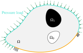
(a)

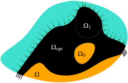
(b)

Figure 1: A schematic diagram for a pressure-loaded problem. (1(a)) Design domain. $\mathrm{\Omega}_{1}$ and $\mathrm{\Omega}_{0}$ denote the non-design solid and void regions, respectively. Fluidic pressure load is indicated via a set of arrows. Fixed boundary conditions are also depicted. (1(b)) A representative solution, $\mathrm{\Omega}_{\text{opt}}$

The applied input (external) load on structures can vary (design-dependent) or remain constant with optimization evolution. Though one encounters the former loads in various applications (Kumar et al., 2020), handling them in a TO framework is a heavy and involved task as their location, magnitude, and/or direction alter with optimization progress. Thus, developing new approaches or using the existing ones may be challenging, resulting in stiff learning curves for beginners and students. In addition, no open education codes for TO with (fluidic) design-dependent pressure loads yet exist in the current state-of-the-art (Wang et al., 2021). Therefore, the paper’s primary aim is to offer a pedagogical MATLAB code and its extensions for topology optimization of strucutres involving design-dependent fluidic pressure loads with all the required ingredients to reduce barriers to beginners’ learning steps and fill the existing gap. And also, we except that the proposed code will provide a basic platform for developing and extending it for different applications involving pressure (pneumatic) loads, e.g., pneumatically activated soft robotics (Xavier et al., 2022; Kumar, 2023), pressurized meta-material, etc.

Providing educational codes on TO for pedagogical purposes is a welcomed trend that commenced with the celebrated 99-line MATLAB code written by Sigmund (2001). An efficient version of 99-line code, top88, is presented in Andreassen et al. (2011). Codes use quadrilateral elements to parameterize the design domains. Such elements provide a node/point connection between two diagonally juxtaposed elements whereas polygonal/hexagonal elements offer non-singular connectivity. Therefore, by and large, geometrical anomalies (checkerboard patterns and point connections) get subdued inherently with such FEs (Saxena, 2011; Talischi et al., 2012; Kumar, 2023). MATLAB codes with polygonal/hexagonal elements are also presented in Saxena (2011); Talischi et al. (2012); Kumar (2023). Several MATLAB codes involving different physics also exist. Andreassen and Andreasen (2014); Xia and Breitkopf (2015) present codes for material modeling using the homogenization method. Gao et al. (2019) provide ConTop2D and ConTop3D MATLAB codes for TO of multiscale 2D and 3D composite structures, respectively. An efficient 137-line TO MATLAB code is provided by Han et al. (2021) for the structures experiencing finite deformation using a bi-directional structural optimization method. Christiansen and Sigmund (2021) present a MATLAB code for inverse design in phonotics. Ferrari et al. (2021) provide a code in MATLAB for linearized buckling in TO. Ali and Shimoda (2022) present a MATLAB code for concurrent topology optimization for lightweight structures with high heat conductivity and stiffness. Readers can find a comprehensive list of educational papers in Wang et al. (2021).

A schematic diagram for the pressure load problem is depicted in Fig. 1(a). A set of arrows indicates the applied pressure load. In a representative optimized design solution (Fig. 1(b)), one can see that the pressure load boundary shifts and settles within the design domain; thus, direction, and loading location alter. Therefore, such loads require a unique modeling technique in a TO framework. Hammer and Olhoff (2000) were the first to model pressure load in a TO framework for designing loadbearing structures. Many approaches have been proposed after that; see Picelli et al. (2019); Kumar et al. (2020); Kumar and Langelaar (2021) for the comprehensive lists. In a typical TO environment with a design-dependent pressure load, an ideal approach is expected to provide suitable solutions to the following challenges (C_i):

• C₁: How to relate the pressure load to the design variables.

• C₂: How to implicitly or explicitly locate bounding surface for applying the pressure load as TO advances

• C₃: How to convert the boundary pressure load (pressure field) to the consistent nodal forces.

• C₄: How to evaluate the load sensitivities efficiently that appear for the design-dependent forces in the sensitivity analysis.

The method in Kumar et al. (2020) employs the Darcy law with a drainage term to relate the pressure load and the design variables (C₁). That, in turn, also helps implicitly identify the pressure-bounding surface, i.e., a solution to C₂. The pressure load is consistently converted to nodal loads using a transformation matrix arising due to the equivalent body force, i.e., the approach takes care of C₃. Further, the method facilitates computationally cheap evaluation of the load sensitivities directly using the adjoint-variable method, i.e., it provides a viable and efficient solution to C₄. Note many previous TO approaches involving pressure loads neglect the load sensitivities that per Kumar et al. (2020) influence the optimized structures’ shape and topology. The approach presented in Kumar et al. (2020) is also suitable for designing pressure-driven compliant mechanisms (Kumar et al., 2020), which is expected to open a potential direction towards developing soft robots using TO (Kumar, 2023). Further, the method is readily extended for optimizing 3D loadbearing designs and pressure-driven compliant mechanisms in Kumar and Langelaar (2021). Therefore, this paper adopts the approach herein for developing the proposed code.

This paper provides a compact 100-line MATLAB code, TOPress, for topology optimization of structures involving fluidic pressure loads using the method of moving asymptotes (MMA, cf. Svanberg (1987)) for educational purposes. Though the MMA MATLAB code contains many lines (Svanberg, 1987), for brevity and compactness, the mmasub function call is counted as two lines in the provided 100-line code (Appendix B). TOPress is developed per the approach proposed by Kumar et al. (2020), and its various extensions are provided to solve benchmark problems. Steps to include a projection filter are also given to achieve close to black-and-white loadbearing structures. As mentioned above, the code uses the MMA (written in 1999 and updated in 2002 version) (Svanberg, 1987) as the optimizer, which can permit users to readily extend the code for various applications involving fluidic pressure loads with multiple constraints and/or different additional physics. In addition, with a design-dependent load, compliance objective may potentially lose its monotonous behavior with respect to the design variables due to load sensitivity terms, and, in such cases, the MMA optimizer is typically preferred (Bruyneel and Duysinx, 2005; Kumar, 2022).

The remainder of the paper is structured as follows. Sec. 2 presents a topology optimization framework—pressure load modeling and nodal load calculation, demonstration of the Darcy law, and optimization problem formulation with sensitivity analysis. Sec. 3 describes MATLAB implementation in detail and provides various extension for benchmark numerical examples. An extension of the 100-line code with the Heaviside projection filter is also provided. Lastly, concluding remarks are noted in Sec. 4.

2 Topology optimization framework

The section describes the modeling of the pressure load, evaluation of the consistent nodal loads, objective formulation, and sensitivity analysis in short. One can refer to Kumar et al. (2020) for a detailed description.

2.1 Pressure load modeling and nodal loads evaluation

As TO advances, the material states of FEs change. Thus, elements can be considered a porous medium at the beginning of TO. In addition, a pressure difference across the design domain is known already from the given pressure load boundary conditions. Therefore, the Darcy law determining the flux of a fluid flow due to pressure difference in a porous medium can be a natural and smart choice for modeling the fluidic pressure load (Kumar et al., 2020). Mathematically, one writes the flux $\mathbf{q}$ using the available pressure gradient $\nabla p$, permeability $\kappa$ of the medium, and the fluid viscosity $\mu$ as

$$\bm{q}=-\frac{\kappa}{\mu}\nabla p=-K(\tilde{\bm{\rho}})\nabla p,$$ (1)

where $\tilde{\bm{\rho}}$, the physical design vector herein, is the filtered design vector (Bruns and Tortorelli, 2001); $K(\tilde{\bm{\rho}})$, the flow coefficient, is defined for element $e$ using the flow contrast $\epsilon=\frac{K_{s}}{K_{v}}$ as

$$K(\tilde{\rho_{e}})=K_{v}\left(1-(1-\epsilon)\mathcal{H}(\tilde{{\rho_{e}}},\,\beta_{\kappa},\,\eta_{\kappa})\right),$$ (2)

where $K_{v}$ and $K_{s}$ are the flow coefficients of the void and solid phases of an element, and $\mathcal{H}(\bar{{\rho_{e}}},\,\beta_{\kappa},\,\eta_{\kappa})=\frac{\tanh{\left(\beta_{\kappa}\eta_{\kappa}\right)}+\tanh{\left(\beta_{\kappa}(\tilde{\rho}_{e}-\eta_{\kappa})\right)}}{\tanh{\left(\beta_{\kappa}\eta_{\kappa}\right)}+\tanh{\left(\beta_{\kappa}(1-\eta_{\kappa})\right)}}$, is a smooth Heaviside function. $\{\eta_{\kappa},\,\beta_{\kappa}\}$ are the flow parameters. $\eta_{\kappa}$ and $\beta_{\kappa}$ define the step position and slope of $K(\tilde{\rho_{e}})$, respectively. We set $K_{v}=1$, and $\epsilon=$1\text{\times}{10}^{-7}\text{\,}$$, i.e., $K_{s}=\epsilon$ (Kumar and Langelaar, 2021) in the provided code, TOPress. To this end, we write $K(\tilde{\rho_{e}})=1-(1-\epsilon)\mathcal{H}(\tilde{{\rho_{e}}},\,\beta_{\kappa},\,\eta_{\kappa})$. Using the fundamentals of the state equilibrium, the balanced equation corresponding to (1) is

$$\nabla\cdot\bm{q}=-\nabla\cdot\left(K(\tilde{\bm{\rho}})\nabla p\right)=0$$ (3)

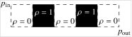
(a)

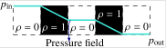
(b)

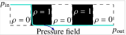
(c)

Figure 2: (2(a)) A test design domain, $p_{\text{in}}$ and $p_{\text{out}}$ are the input and output fluidic pressure, respectively. (2(b)) The obtained pressure field variation from the solution of the Darcy law (Eq. 3), and (2(c)) The desired pressure field variation.

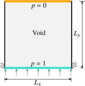
(a) SP1

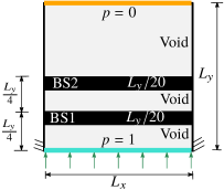
(b) SP2

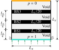
(c) SP3

Figure 3: Three sample problems (SP1, SP2, SP3) demonstrate the working of the Darcy law. $L_{x}\times L_{y}=$200\text{\,}$\times$200\text{\,}$$. Pressure loads of $1\text{\,}$ and $0\text{\,}$ are applied on the bottom and top edges, respectively. Strips in black with width $\frac{L_{y}}{20}$ are with $\rho=1$.

Figure 4: Pressure colorbar. ${p}_{\text{max}}=$1\text{\,}$$ and $p_{\text{min}}=$0\text{\,}$$.

(a) SP1 P-field

with DrainT=0 or 1

(b) SP2 P-field

with DrainT=0

(c) SP2 P-field

with DrainT=1

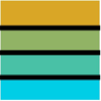
(d) SP3 P-field

with DrainT=0

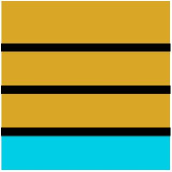
(e) SP3 P-field

with DrainT=1

Figure 5: Pressure field (P-field) plots.

(a) P-field

(b) Nodal forces

Figure 6: P-field and nodal forces along the vertical central line for SP2.

(a) P-field

(b) Nodal forces

Figure 7: P-field and nodal forces along the vertical central line for SP3.

One solves (3) using the standard finite element method to determine the pressure field across the given design domain. The given design domain is depicted in Fig. 2(a). $p_{\text{in}}$ and $p_{\text{out}}=0$ are the input and output fluidic pressure, respectively. With the Darcy law solution (3) and the given pressure load boundary conditions, the obtained pressure field for this problem (Fig. 2(a)) is as displayed in Fig. 2(b), which is physically unrealistic as the pressure gradient exists across the solid regions ($\rho=1$). Thus, to achieve the natural and desired pressure field/distribution, a conceptualized volumetric drainage per second in a unit volume term, $Q_{\text{drain}}$, with the Darcy law is used (Kumar et al., 2020). $Q_{\text{drain}}$ acts as a pressure drainer from the solid elements. The final balance equation in conjunction with $Q_{\text{drain}}$ can be written as (Kumar et al., 2020)

$$\nabla\cdot\bm{q}-Q_{\text{drain}}=\nabla\cdot\left(K(\tilde{\bm{\rho}})\nabla p\right)+Q_{\text{drain}}=0.$$ (4)

${Q}_{\text{drain}}=-D(\bar{\rho_{e}})(p-p_{\text{ext}})$ with $D(\bar{\rho_{e}})=D_{\text{s}}\mathcal{H}(\bar{{\rho_{e}}},\,\beta_{d},\,\eta_{d})$. $\left\{\eta_{\text{d}},\,\beta_{\text{d}}\right\}$ are the drainage parameters. Note, $D_{\text{s}}=\left(\frac{\ln{r}}{\Delta s}\right)^{2}K_{\text{s}}$, where $r=\frac{p|_{\Delta s}}{p_{\text{in}}}$; $\Delta s$, a penetration parameter, is set to width/height of a few FEs, and $p|_{\Delta s}$ is the pressure at $\Delta s$. Based on our experience, $r\in[0.001\,\,0.1]$. For all practical purposes and to reduce the number of user-defined parameters, we consider $\eta_{h}=\eta_{k}=\eta_{f}$ and $\beta_{h}=\beta_{k}=\beta_{f}$ in the provided code TOPress. However, one can choose them differently per the recommendation outlined in Kumar et al. (2020). In a discrete setting, using the standard finite element steps, (4), for element $i$, yields considering $p_{\text{out}}=0$ and $\mathbf{q}_{\mathrm{\Gamma}}=0$ to (Kumar et al., 2020)

$$\left[\int_{\Omega_{e}}\left(K~{}\mathbf{B}^{\top}_{\text{p}}\mathbf{B}_{\text{p}}\right)\text{d}V+\int_{\Omega_{e}}\left(D~{}\mathbf{N}^{\top}_{\text{p}}\mathbf{N}_{\text{p}}\right)\text{d}V~{}\right]\mathbf{p}_{e}=\mathbf{0},$$ (5)

where $\mathbf{N}_{\text{p}}=[N_{1},\,N_{2},\,N_{3},\,N_{4}]^{\top}$ are the bilinear shape functions for the quadrilateral elements employed to parameterized the design domains, $\mathbf{B}^{\top}_{\text{p}}=\nabla\mathbf{N}_{\text{p}}$, and $\mathbf{p}_{e}=[p_{1},\,p_{2},\,p_{3},\,p_{4}]^{\top}$. Note $N_{i}$ and $p_{i}$ ($i=1,\,\cdots,\,4$) represent the shape function and pressure degree of freedom for the $i^{\text{th}}$ node of element $e$, respectively (see Fig. 9(b)). In light of numerical integration, (5) yields to

$$\mathbf{K}_{\text{p}}^{e}\mathbf{p}_{e}+\mathbf{K}^{e}_{\text{Dp}}\mathbf{p}_{e}=\mathbf{A}_{e}\mathbf{p}_{e}=\mathbf{0},$$ (6)

where $\mathbf{\mathbf{K}}_{\text{p}}^{e}$ and $\mathbf{K}^{e}_{\text{Dp}}$ are the element flow matrices due to the Darcy law and the drainage term, respectively (See Appendix A). $\mathbf{A}_{e}$ indicates the overall element flow matrix. At the global level, (6) transpires to

$$\mathbf{Ap}=\mathbf{0},$$ (7)

where $\mathbf{p}$ and $\mathbf{A}$ are the global pressure vector and flow matrix, respectively. Note, $\mathbf{A}$ is obtained by assembling $\mathbf{K}_{\text{p}}^{i}$ and $\mathbf{K}^{i}_{\text{Dp}}$. The solution to (7) gives the pressure field $\mathbf{p}$ as a function of the design variables. To this end, when the problem shown in Fig. 2(a) is solved using (7), one obtains the pressure field as indicated in Fig. 2(c), which is indeed a realistic pressure distribution.

Further, the obtained $\mathbf{p}$ is expressed as an equivalent body force using the balance equation, which gives (Kumar et al., 2020)

$$\bm{b}\text{d}V=-\nabla p\text{d}V,$$ (8)

where $\bm{b}$ is the body force per unit volume. In view of the standard finite element methods, (8) provides

$$\mathbf{F}_{e}=-\left[\int_{\mathrm{\Omega}_{e}}{\mathbf{N}}^{\!\top}_{\mathbf{u}}\mathbf{B}_{p}d{V}\right]\,\mathbf{p}_{e}=\mathbf{T}_{e}\,\mathbf{p}_{e},$$ (9)

where $\mathbf{N}_{\mathbf{u}}=[N_{1}\mathbf{I},\,N_{2}\mathbf{I},\,N_{3}\mathbf{I},\,N_{4}\mathbf{I}]$, with $\mathbf{I}$ the identity matrix in $\mathcal{R}^{2}$. In global sense, (8) yields to

$$\mathbf{F}=-\mathbf{T}\mathbf{p},$$ (10)

where $\mathbf{T}$ is the global transformation matrix, and $\mathbf{F}$ is the global force vector.

To summarize, (7) is used for determining the pressure field, whereas the corresponding consistent nodal force vector for an element is calculated using (9).

2.2 Demonstration of the Darcy law

To demonstrate success of the Darcy law with drainage term, we consider a set of three problems, SP1, SP2, and SP3, shown in Fig. 3. SP1 is considered fully void, whereas SP2 and SP3 contain two and three solid bars of width $\frac{L_{y}}{20}$ each. We use $L_{x}$ and $L_{y}$ to represent the dimensions of the designs in $x-$ and $y-$directions, respectively. $L_{x}=$200\text{\,}$$ and $L_{y}=$200\text{\,}$$ are set. The out of plane thickness, t, is set to $1\text{\,}$. The bottom edges of the domains experience $\texttt{Pin}=$1\text{\,}$$ pressure load, whereas their top edges are placed on zero pressure load. The bottom parts of the left and right edges are fixed. The domains are parameterized by $\texttt{nelx}\times\texttt{nely}=\texttt{nel}=200\times 200$ square bi-linear finite elements, where nelx and nely indicate number of the squared finite elements (FEs) in $x-$ and $y-$directions, respectively. nel is the total number of finite elements used to parameterize the design domains. Fig. 4 provides the color scheme used to display the pressure variation for the problems.

Figure 5 shows the pressure field (P-field) variation for SP1, SP2, and SP3. For SP2 and SP3, two cases are considered–with drainage term (DrainT=1) and without drainage term (DrainT=0). Fig. 5(b) and Fig. 5(d) display pressure variation for SP2 and SP3 with DrainT=0, respectively . They are unrealistic pressure variations, as one can observe a pressure gradient across the solid strips. A realistic pressure distribution (no pressure gradient across the solid bars) can be noted with DrainT=1 (Fig. 5(c) and Fig. 5(e)). The pressure field (P-field) and nodal forces along the vertical central line are plotted in Fig. 6 for SP2. One again notes an unrealistic pressure field with DrainT=0 (Fig. 5(d)). The variation of pressure and nodal forces along the central line of SP3 are displayed in Fig. 7(a) and Fig. 7(b), respectively. For all the sample problems, we find $\texttt{MFx}=$0.0\text{\,}$$ and $\texttt{MFy}=$200.0\text{\,}$$. $x-$ and $y-$ magnitudes of the forces are indicated by MFx and MFy, respectively. The force applied by the given pressure load is $\texttt{Pin}\times\texttt{t}\times{L_{x}}=1\times 1\times 200=$200\text{\,}$$ in the vertical direction, which equals to MFy, and that indeed proves the correctness of the pressure load modeling. Therefore, herein it gets established that the Darcy formulation with the drainage term ($\texttt{DrainT}=1$) gives the realistic pressure field while maintaining the force magnitude. With regard to this study, TOPress uses DraintT=1, as default. Next, we present the topology optimization formulation for the compliance minimization problem with the above-described Darcy law.

2.3 Topology optimization formulation

We present TOPress code for the compliance minimization with the given volume fraction for the loadbearing structures. The optimization problem can be written as

$$\left.\begin{aligned} \hfil\displaystyle\begin{split}&{\min_{\tilde{\bm{\rho}}}}\quad C({\tilde{\bm{\rho}}})=\mathbf{u}^{\top}\mathbf{K}(\tilde{\bm{\rho}})\mathbf{u}=\sum_{j=1}^{\mathtt{nel}}\mathbf{u}_{j}^{\top}\mathbf{k}_{j}(\rho_{j})\mathbf{u}_{j}\\ &\text{subjected to:}\\ &\bm{\lambda}_{1}:\,\,\mathbf{A}\mathbf{p}=\mathbf{0}\\ &\bm{\lambda}_{2}:\,\,\mathbf{K}\mathbf{u}=\mathbf{F}=-\mathbf{T}\mathbf{p}\\ &\Lambda:V(\tilde{\bm{\rho}})-V^{*}\leq 0\\ &\quad\,\,\,\,\bm{0}\leq\bm{\rho}\leq\bm{1}\\ &\text{Data:}\quad V^{*},\,E_{0},\,E_{\text{min}},\,p,\,K_{v},\,\epsilon\end{split}\end{aligned}\right\},$$ (11)

where $C$ indicates the structure’s compliance and nel is the total number of elements used to describe the design domain. $\mathbf{u}$ and $\mathbf{K}$ represent the global displacement vector and stiffness matrix, respectively. $V^{*}$ indicates the permitted resource, and $V$ represents the current volume of the evolving domain. $\mathbf{F}$, the global force vector, appears due to the pressure loads. $\bm{\lambda}_{1}$ (vector), $\bm{\lambda}_{2}$ (vector) and $\Lambda$ (scalar) are the Lagrange multipliers. $\tilde{\bm{\rho}}$ is the filtered design vector corresponding to the actual design variable vector $\bm{\rho}$. We use the classical density filter (Bruns and Tortorelli, 2001) in the provided codes. The filtered design variable for element $i$ is determined as:

$$\tilde{\rho}_{i}=\frac{\displaystyle\sum_{j=1}^{\texttt{nel}}\rho_{j}\mathrm{v}_{j}\mathrm{w}(\mathbf{x}_{i},\mathbf{x}_{j})}{\displaystyle\sum_{j=1}^{\texttt{nel}}\mathrm{v}_{j}\mathrm{w}(\mathbf{x}_{i},\mathbf{x}_{j})}\;,$$ (12)

where weight $\mathrm{w}(\mathbf{x}_{i},\mathbf{x}_{j})$ = $\mathrm{max}\left(0\;,\;1-\frac{\|\mathrm{\mathbf{x}}_{i}-\mathrm{\mathbf{x}}_{j}\|}{\mathrm{r}_{\mathrm{fill}}}\right)$ (Bruns and Tortorelli, 2001). $r_{\text{fill}}$ is the filter radius. $\mathrm{v}_{j}$ is the volume of element $j$. Note that $\mathrm{v}_{j}$ and $\mathrm{w}(\mathrm{x}_{i},\mathrm{x}_{j})$ do not alter with TO iterations; thus, they are determined once at the beginning of the optimization and are stored in a matrix $\mathbf{H}$ as:

$$\mathrm{H}_{i,j}=\frac{\mathrm{v}_{j}\>\mathrm{w}(\mathrm{\mathbf{x}}_{i},\mathrm{\mathbf{x}}_{j})}{{\displaystyle\sum_{j=1}^{\texttt{nel}}\mathrm{v}_{j}\mathrm{w}(\mathrm{\mathbf{x}}_{k},\mathrm{\mathbf{x}}_{j})}}\>.$$ (13)

To this end, one writes the filtered design vector as $\bm{\tilde{\rho}}=\mathbf{H}\bm{\rho}$ and its derivative as $\frac{\partial\bm{\tilde{\rho}}}{\partial\bm{\rho}}=\mathbf{H}^{\top}$. We perform the filtering using imfilter MATLAB function in the 100-line code (see Appendix B). Note that one may also use sensitivity filtering as per Sigmund (2001).

At each TO iteration, $\mathbf{u}$ is determined by solving the structure state equation, $\mathbf{K}\mathbf{u}=\mathbf{F}=-\mathbf{T}\mathbf{p}$, wherein $\mathbf{p}$ is the solve of fluid flow equilibrium $\mathbf{Ap}=\mathbf{0}$, and $\mathbf{T}$ is the transformation matrix as described above. Stiffness matrix $\mathbf{K}$ depends upon the physical design variables wherein the modified solid Isotropic Material with Penalization (SIMP) scheme (Sigmund, 2007) is employed to interpolate Young’s modulus of element $i$. Mathematically,

$$\mathrm{E}_{i}=\mathrm{E}_{\mathrm{min}}+\tilde{\rho}^{p}_{i}(\mathrm{E}_{0}-\mathrm{E}_{\mathrm{min}}),$$ (14)

where $p$, the SIMP parameter encourages convergence of TO towards 0-1 solutions. $E_{0}$ and $E_{\text{min}}$ are Young’s moduli of the solid and void states of an element, respectively, and $E_{i}$ is Young’s modulus of element $i$.

2.3.1 Sensitivity analysis

The presented 100-line code and its extensions employ a gradient-based optimizer, the method of moving asymptotes (MMA, cf. Svanberg (1987)), to solve the optimization problem (11). Therefore, derivatives of the objective and constraints with respect to design variables are required. We use the adjoint-variable method to determine the sensitivities by evaluating the Lagrange multipliers corresponding to the balance equations. Typically, one uses the adjoint-variable method wherein the number of design variables exceeds the number of constraints/state-dependent responses. The augmented performance function $\mathcal{L}$ is defined using the objective function and equilibrium equations (11) as

$$\mathcal{L}=\mathbf{u}^{\top}\mathbf{K}\mathbf{u}+\bm{\lambda}_{1}^{\top}\mathbf{AP}+\bm{\lambda}_{2}^{\top}\left(\mathbf{KU+TP}\right).$$ (15)

Differentiating (15) with respect to physical variables, that yields

$$\begin{split}\frac{d\mathcal{L}}{d\tilde{\bm{\rho}}}=&2\mathbf{u}^{\top}\mathbf{K}\frac{\partial\mathbf{u}}{\partial\tilde{\bm{\rho}}}+\mathbf{u}^{\top}\frac{\partial\mathbf{K}}{\partial\tilde{\bm{\rho}}}\mathbf{u}+\bm{\lambda}_{1}^{\top}\left(\frac{\partial\mathbf{A}}{\partial\tilde{\bm{\rho}}}\mathbf{p}\right)+\bm{\lambda}_{1}^{\top}\left(\mathbf{A}\frac{\partial\mathbf{p}}{\partial\tilde{\bm{\rho}}}\right)\\ &+\bm{\lambda}_{2}^{\top}\left(\frac{\partial\mathbf{K}}{\partial\tilde{\bm{\rho}}}\mathbf{u}+\mathbf{K}\frac{\partial\mathbf{u}}{\partial\tilde{\bm{\rho}}}\right)+\bm{\lambda}_{2}^{\top}\left(\frac{\partial\mathbf{T}}{\partial\tilde{\bm{\rho}}}\mathbf{p}+\mathbf{T}\frac{\partial\mathbf{p}}{\partial\tilde{\bm{\rho}}}\right)\\ =&\mathbf{u}^{\top}\frac{\partial\mathbf{K}}{\partial\tilde{\bm{\rho}}}\mathbf{u}+\bm{\lambda}_{2}^{\top}\left(\frac{\partial\mathbf{K}}{\partial\tilde{\bm{\rho}}}\mathbf{u}\right)+\bm{\lambda}_{1}^{\top}\left(\frac{\partial\mathbf{A}}{\partial\tilde{\bm{\rho}}}\mathbf{p}\right)\\ &+\underbrace{\left(2\mathbf{u}^{\top}\mathbf{K}+\bm{\lambda}_{2}^{\top}\mathbf{K}\right)}_{\Theta_{1}}\frac{\partial\mathbf{u}}{\partial\tilde{\bm{\rho}}}+\underbrace{\left(\bm{\lambda}_{1}^{\top}\mathbf{A}+\bm{\lambda}_{2}^{\top}\mathbf{T}\right)}_{\Theta_{2}}\frac{\partial\mathbf{p}}{\partial\tilde{\bm{\rho}}}\end{split}$$ (16)

In light of the fundamentals of the adjoint-variable method, we select $\bm{\lambda}_{1}$ and $\bm{\lambda}_{2}$ such that $\Theta_{1}=0$ and $\Theta_{2}=0$, which give

$$\bm{\lambda}_{2} =-2\mathbf{u},$$ (17)

$$\bm{\lambda}_{1}^{\top} =-\bm{\lambda}_{2}^{\top}\mathbf{T}\mathbf{A}^{-1}=2\mathbf{u}^{\top}\mathbf{T}\mathbf{A}^{-1},$$

and

$$\frac{d{C}}{d\tilde{\bm{\rho}}}=-\mathbf{u}^{\top}\frac{\partial\mathbf{K}}{\partial\tilde{\bm{\rho}}}\mathbf{u}+\underbrace{2\mathbf{u}^{\top}\mathbf{T}\mathbf{A}^{-1}\frac{\partial\mathbf{A}}{\partial\tilde{\bm{\rho}}}\mathbf{p}}_{\text{Load sensitivities}}$$ (18)

One notes, the load sensitivities modify the total sensitivities of compliance. With a constant load case, the compliance sensitivities contain only the first term of (18). The load sensitivity terms affect the monotonous behavior of the compliance objective of the design problem with the design-dependent loads (Kumar, 2022). Finally, one can use the chain rule to determine the derivatives of the objective with respect to the design variables as

$$\frac{d{C}}{d\bm{\rho}}=\frac{d{C}}{d\tilde{\bm{\rho}}}\frac{d\tilde{\bm{\rho}}}{d\bm{\rho}}$$ (19)

The derivative of the volume constraint is calculated per Sigmund (2001), which is straightforward. Having discussed all the ingredients needed for the pressure load formulation in a density-based TO formulation, next, we present the MATLAB implementation for the 100-line code and its various extensions for different pressure-loaded problems.

3 MATLAB Implementation

The internally pressurized arch design is the classical problem in TO with design-dependent pressure load. The problem was first presented and solved by Hammer and Olhoff (2000). Many researchers also consider the problem to test their method after that, e.g., Chen and Kikuchi (2001); Du and Olhoff (2004); Sigmund and Clausen (2007); Zhang et al. (2008); Xia et al. (2015); Picelli et al. (2015); Emmendoerfer Jr et al. (2018); Picelli et al. (2019); Neofytou et al. (2020); Kumar et al. (2020); Ibhadode et al. (2020); Huang et al. (2022), to name a few. Thus, we consider the arc problem to demonstrate the presented 100-line MATLAB code, TOPress. The design domain, pressure, and structure boundary conditions for the internally pressurized arch are displayed in Fig. 8.

One calls TOPress from the MATLAB prompt as

⬇

TOPress(nelx,nely,volf,penal,rmin,etaf,betaf,lst,maxit)

where volf is the permitted volume fraction, penal is the SIMP penalization parameter $p$, rmin is the filter radius $r_{\text{fill}}$, etaf denotes both (the step position) $\eta_{\kappa}$ and $\eta_{d}$ (Sec. 2.1), betaf indicates $\beta_{\kappa}$ and $\beta_{d}$ (Sec. 2.1) and maxit is the maximum number for the MMA optimizer. lst determines participation of load sensitivities in (18), i.e., $\texttt{lst}=1$ indicates load sensitivities are included, whereas $\texttt{lst}=0$ implies otherwise.

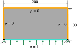
Figure 8: Internally pressurized arch design. Pressure load is applied on the bottom edges, whereas remaining edges are fixed at 0 pressure.

TOPress primarily contains the following six parts:

• PART 1: MATERIAL AND FLOW PARAMETERS

• PART 2: FINITE ELEMENT ANALYSIS PREPARATION and NON-DESIGN DOMAIN

• PART 3: PRESSURE & STRUCTURE B.C’s, LOADs

• PART 4: FILTER PREPARATION

• PART 5: MMA OPTIMIZATION PREPARATION

• PART 6: MMA OPTIMIZATION LOOP

which are described in detail below.

PART 1 records the material and flow parameters (lines 2-7). $\mathtt{E1}$ is Young’s modulus $E_{1}$ of the material, $\mathtt{Emin}$ is the Young’s modulus assigned to the void elements to avoid numerical issues, and the Poisson’s ratio is indicated via nu. Kv is the flow coefficient of void element, $K_{v}$, epsf is the flow contrast $\epsilon$, Dels is the penetration depth $\Delta s$, Ds is the drainage parameter $D_{s}$, and kvs is $K_{v}(1-\epsilon)$. Note, Kv is set to 1, therefore ${K_{s}}=\epsilon$, i.e., $K_{s}=\texttt{epsf}$.

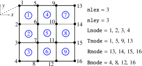
(a) Mesh grid nomenclature: Global format

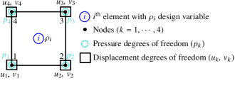
(b) Nomenclature for element $i$: Local format

Figure 9: Nomenclature for element $i$ and a mesh grid are displayed. Each node is characterized by two displacements and one pressure degree of freedom. nelx and nely are the number of elements used in $x-$ and $y-$directions, respectively. Lnode, Tnode, Rnode and Bnode indicate arrays of nodes constituting the left, top, right and bottom edges, respectively.

PART 2 provides finite element analysis preparation steps (lines 8-33). Figure 9(a) displays terminology and style for nodes and elements numbering employed for the discretized domains. The local nomenclature and numbering for element $i$ are depicted in Fig. 9(b). $\rho_{i}$ is the design variable that is considered constant within element $i$ and thus, its physical density $\tilde{{\rho_{i}}}$ (Sec. 2.3). Each element poses four nodes and two and one degrees of freedom (DOFs) per node for the displacement and pressure fields, respectively (Fig. 9(b)). Node $k$ poses $2k-1$ and $2k$ DOFs for the displacement in $x-$ and $y-$directions, respectively. The node number indicates the respective pressure DOF. The total number of elements and nodes are evaluated on line 9, which are denoted via nel and nno, respectively. Lines 10-12 are as per Andreassen et al. (2011) where matrix Udof contains element-wise displacement DOFs. Row $i$ of Udof gives the DOFs of nodes of element $i$.

Nodes constituting the left, top, right, and bottom edges of the domains are recorded in arrays Lnode, Tnode, Rnode and Bnode, respectively (lines 13-14). Element-wise pressure DOFs are recorded in Pdofs (line 15). Arrays allPdofs and allUdofs record pressure and displacement DOFs of the parameterized domains. Vectors iP and jP record the rows and columns indices for the flow matrix using Pdofs and nel (lines 16-17). Likewise, $\left\{\texttt{iT,\,jT}\right\}$ and $\left\{\texttt{iK,\,jK}\right\}$ contain the rows and columns indices for the transformation and stiffness matrices, respectively (lines 18-21). These vectors are defined per Andreassen et al. (2011) as described for $\left\{\texttt{iK,\,jK}\right\}$.

Next, Kp determines the element Darcy flow matrix $\mathbf{K}_{\text{p}}^{e}$ (6) with unit flow coefficient on line 22. Likewise, KDp evaluates the element drainage matrix $\mathbf{K}_{\text{DP}}^{e}$ (6) with unit $D_{s}$ on line 23. Lines 25-29 provide a routine to determine the element stiffness matrix with unit Young’s modulus on line 29 per Andreassen et al. (2011). Lines 30-33 provide a function handle for the Heaviside function and its derivative. Line 34 records the elements constituting non-design solid and non-design void regions in NDS and NDV, respectively. act determined on line 35 contains the active set of elements.

PART 3 describes the boundary conditions for the flow and structure settings (lines 36-44). PF and Pin contain the initialize pressure vector and input pressure load (line 37). Line 38 applies the given pressure loading conditions for the arc problem. One needs to modify this line as per the different problems. The fixed pressure DOFs and the given corresponding pressure values are recorded in vectors fixedPdofs and pfixeddofsv, respectively. Vector fixedUdofs (line 42) contains the displacement DOFs, and corresponding free DOFs are determined on line 43 (vector freeUdofs). Line 44 initializes the displacement vector $\mathbf{u}$ and the Lagrange multiplier $\bm{\lambda}_{1}$ (11).

PART 4 provides filter preparation per Ferrari et al. (2021) using the in-built imfilter function (lines 45-48). The function allows to specify zero-Dirichlet or zero-Neumann boundary conditions. Here, we use the former, the default option for imfilter.

PART 5 provides MMA optimization preparation, initialization, and allocations for some variables (lines 49-58). x (line 50) and xphys (line 52) denote the actual and physical design variables, respectively. Vector x is first initialized to a zero vector (line 50). Then it is updated per the non-design solid and void regions (line 51), i.e., for the active set of elements. Variables mentioned on lines 52-57 are specifically related to the MMA optimizer (Svanberg, 1987). Scalars nMMA and mMMA indicate the number of active design variables and constraints, respectively (line 52). The design variable vector for the MMA is denoted by xMMA, which is initialized to the active design variable vector, x(act). xphys is initialized on line 52. mvLt (line 52) is the external move limit for the MMA optimizer. On line 53, the minimum and maximum values of the design vector are defined by xminvec and xmaxvec, respectively. Vectors low and upp contain the lower and upper limits of the design variables, respectively (line 54). The MMA constants, cMMA, dMMA, a0 and aMMA are defined on line 55. Vectors xold1 and xold2 contain the old value of the design vector xMMA, which are initialized on line 56. The optimization loop counter is recorded in loop (line 57), and the absolute change in the design vector is read in change (line 57). The derivative of the volume constraint dvol0 is determined on line 50 and filtered on line 58, which is recorded in dvol.

PART 6 is executed on lines 59-100 and contains five sub-parts. All variables within this part are repeatedly determined within the optimization loop. sparse function is employed for assembling the element flow, transformation and stiffness matrices using the vectors $\left\{\texttt{iP,\,jP}\right\}$, $\left\{\texttt{iT,\,jT}\right\}$, and $\left\{\texttt{iK,\,jK}\right\}$, respectively.

Subpart 6.1 solves the flow balance equation (7) on lines 62-69. Using the Heaviside function handle (line 30), the flow (Kc) and drainage (Dc) coefficients of elements are determined on line 63 and line 64, respectively. Kc and Dc indicate $K$ and $D$ (4), respectively. The design-dependent flow vector is determined on line 65. Kp and KDp are converted into column vectors, are multiplied respectively by Kc (flow coefficient K (2)) and Dc (Drainage term D (4)) and then added to evaluate flow vector Ae. The global flow matrix AG (used to represent $\mathbf{A}$ (7)) is determined on line 66 by placing Ae vector as third entries. Line 66 determines the flow matrix Aff that corresponds to free pressure DOFs. PF, i.e., $\mathbf{p}$ (7) is evaluated on line 67 using decomposition MATLAB function. On line 69, the vector PF is modified per the given pressure boundary conditions.

Subpart 6.2 solves the structure balance equation (lines 70-77). The first part determines the global transformation matrix $\mathbf{T}$ (10) denoted via TG (line 72) from the vector Ts. Ts is evaluated by converting $\mathbf{T}_{e}$ (9) indicated by Te matrix into a column vector and appropriately reshaping it (line 71). The global consistent force vector is determined on line 73. Design-dependent Young’s modulus vector E is determined on line 74. The stiffness vector Ks (line 75) is evaluated as Ae (line 65) using element stiffness matrix ke and E. The global stiffness matrix $\mathbf{K}$ indicated via KG is determined on line 76. The global displacement vector $\mathbf{u}$ denoted by U is determined on line 77 using the decomposition function with Cholesky.

Subpart 6.3 determines the objective, its sensitivities, and volume constraint (lines 78-87). Compliance (11) of the domain is minimized that is evaluated on line 79. Vector lam1 indicate the Lagrange multiplier $\bm{\lambda}_{1}$ (17) which is determined on line 80. Note that $\bm{\lambda}_{2}$ equals to -$2\mathbf{u}$. Vector objsT1 contains the first term of the right-hand side of (18). Note that line 82 and line 83 evaluate the sensitivity terms pertaining to the Darcy flow and drainage term, respectively. These are added to determine objsT1. Likewise, the load sensitivities are evaluated and recorded in vector objsT2 (line 84). Vector objsens (line 84) contains the total objective sensitivities (18). The volume constraint is determined on line 85 (scalar Vol). We normalize the objective and hence its sensitivities. The normalization scalar normf is determined on line 86 using the initial (loop=1) objective value. Objective sensitivities are filtered with normalization on line 87. However, one can prefer to perform normalization after evaluating the filtered sensitivities.

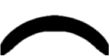
(a) $C=36.25$

(b)

Figure 10: Optimized designs for internally pressurized arch structure with lst=1. (10(a)) Optimized arch design and (10(b)) Optimized material layout with the final pressure field

Subpart 6.4 executes the optimization and updates of the design variables (lines 88-96). The mmasub (line 91) function is called wherein xval is initialized to xMMA. Vectors xminvec and xmaxvec are updated on line 90 using mvLt, the external move limit (line 52). On line 92, vectors xold2, xold1 and xnew are updated using the deal MATLAB function. Line 95 updates the vectors xMMA and xphys using the new solution xnew provided by the MMA, and determines the filtered design variables. On line 96, xphys is updated with respect to the non-design solid and void elements.

We use MMA (mmasub) MATLAB code written in 1999 and updated in 2002 by Svanberg (1987). The optimized structures may remain the same; however, their final objective values may differ (a little) due to numerical calculations and different parameter values used inside the MMA code if one uses a different version of the MMA. One can also choose to define (PART 4) and apply (lines 58, 87, 95) the density filtering in a classical manner per Sigmund (2001); Andreassen et al. (2011) and thereof, may get (slightly) different final objective values for the optimized designs due to numerical calculations and approximations.

subpart 6.5 prints and plots the results using the fprintf and imagesc (lines 97-99). To print the material distribution with the pressure field, one can place the following lines of code below the end of TOPress:

⬇

[xx,yy,nod_dV] = deal(0:nelx, 0:-1:-nely,zeros(nno,1));

convert =[1; 1/2*ones(nely-1,1);1;reshape([1/2*ones(nelx-1,1),1/4*ones(nelx-1,nely-1)...

,1/2*ones(nelx-1,1)]’,[],1);1; 1/2*ones(nely-1,1); 1];

PFP = figure(2); set(PFP,’color’,’w’);

for i = 1:nel, nod_dV(Pdofs(i,:)) = nod_dV(Pdofs(i,:)) + xphys(i); end

xphysnodal = full(reshape(nod_dV.*convert,nely+1,nelx+1)); % nodal density grid

PnodMat = -full(reshape((PF)/Pin, nely+1, nelx+1));% nodal pressure field

winter1 = [ linspace(0,0.85)’ linspace(0.8078,0.65)’ linspace(0.9,0.15)’]; % colorbar style

colormap([winter1; 0. 0. 0. ]); black = 0.01* ones(nely+1, nelx+1);

PrDenHand = surf(xx,yy,PnodMat, ’FaceColor’, ’interp’); caxis([-1 0.0]);hold on

Hbl = imagesc(xx, yy, black, [-1 0.01]); shading interp;xlim ([0 nelx]); ylim([-nely, 0]); view(0,90);

PwDenHand = Hbl; axis equal off; set(PwDenHand, ’AlphaData’, xphysnodal); hold on;

set(PrDenHand, ’CData’, PnodMat); set(PrDenHand,’ZData’,PnodMat);

Next, we solve the internally pressurized arch structure by TOPress and then, the 100-line code is modified for different problems.

3.1 The internally pressurized arch design

To get the optimized designs for the loadbearing arch design (Fig. 8), we call TOPress as

⬇

TOPress(nelx,nely,volf,penal,rmin,etaf,betaf,lst,maxit)

with the following data. $\texttt{nelx}=200$, nely=100, $\texttt{volf}=0.30$, $\texttt{penal}=3$, $\texttt{rmin}=2.4$, $\texttt{etaf}=0.2$, $\texttt{betaf}=8$, $\texttt{lst}=1$ (load sensitivities are included), $\texttt{maxit}=100$ and change$>0.01$ are set.

The optimized arch design, the final P-field with the optimum material layout and convergence curve are depicted in Fig. 10(a), Fig. 10(b) and Fig. 11, respectively. The arch problem is converged at 97${}^{\text{th}}$ MMA iteration. Note that for plotting the final pressure field with the optimized material layout, the code mentioned above is inserted at the end of the 100-line code. The objective convergence is smooth and rapid (Fig. 11). The volume constraint is satisfied and remains active at the end of the optimization (Fig. 11).

Next, we present a study with different volume fractions with and without load sensitivity terms to understand their effects on the optimized designs. We use four volume fractions, volf =0.05, 0.1, 0.25,  and 0.5. $\left\{\texttt{etaf,\,betaf}\right\}$ are set to $\left\{\texttt{volf},\,6\right\}$ (Kumar et al., 2020). Other parameters are taken the same as employed above.

Figure 11: Convergence plot for the internally pressurized arch problem

volf=0.05

$C=1.12,\,\texttt{lst}=1$

volf=0.05

$C=1.14,\,\texttt{lst}=0$

volf=0.1

$C=3.43,\,\texttt{lst}=1$

volf=0.1

$C=3.57,\,\texttt{lst}=0$

volf=0.25

$C=23.58,\,\texttt{lst}=1$

volf=0.25

$C=24.62,\,\texttt{lst}=0$

volf=0.5

$C=135.14,\,\texttt{lst}=1$

volf=0.5

$C=135.80,\,\texttt{lst}=0$

Figure 12: Optimized designs for internally pressurized arch structures for various volume fractions with lst=1 and lst =0.

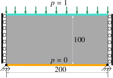
(a)

(b) $C=14.48,\,\texttt{lst}=1$

(c) $C=15.30,\,\texttt{lst}=0$

Figure 13: The design domain, pressure and displacement boundary conditions for the bridge-like structure is depicted in (13(a)). Optimized results with lst=1 and lst=0 are displayed in (13(b)) and (13(c)), respectively.

The optimized designs of the arch structure with (lst=1) and without (lst=0) load sensitivities are displayed in Fig. 12. One can note that optimized designs obtained with lst=1 are relatively stiffer, i.e., high performing (lowered in height) than their counterparts obtained with lst=0. Though the final topologies with lst=1 and with lst=0 are, by and large, same for this problem, and their performances are also close to each other, neglecting load sensitivities (18) may not be a good idea. This gets readily confirmed by other forthcoming numerical examples presented below. The difference in the height of the arch designs is directly related to the final compliance difference for lst=0 and lst=1. TOPress provides good results even for relatively low volume fraction (Fig. 12). One can note that $C$ increases with the volume fraction, which should be the case. Next, we modify TOPress as per the pressure and displacement boundary conditions of different problems of interest.

3.2 Bridge-like pressure loadbearing structure

Figure 13(a) displays the design domain, pressure, and displacement boundary conditions for a bridge-like loadbearing structure per Du and Olhoff (2004). Pressure load is applied on the top edge, whereas the bottom edge is assigned zero pressure load. Left and right edges are permitted to move in the vertical direction. For this problem, one needs to make the following modifications in TOPress. Line 38 is changed to

⬇

PF(Bnode) = 0; PF(Tnode) = Pin; % applying pressure load

and line 42 is altered to

⬇

fixedUdofs = [2*Bnode(1)-1 2*Bnode(1) 2*Bnode(end)-1 2*Bnode(end) 2*Lnode-1 2*Rnode-1]; %fixed displ.

With the above changes, the optimized design depicted in Fig. 13(b) and Fig. 13(c) respectively are obtained by the following call:

⬇

TOPress(200,100,0.20,3,2.5,0.20,10,1,150)

and

⬇

TOPress(200,100,0.20,3,2.5,0.20,10,0,150).

The structure obtained with lst=1 (Fig. 13(b)) is stiffer (high performing) and has less arch height than that obtained with lst=0 (Fig. 13(c)). The observation is similar to what we find for internally pressurized arch structures. In addition, they have different topologies (Fig. 13(b) and Fig. 13(c)). Thus, load sensitivities affect the final topology and can help improve the performance of the optimized designs.It may happen that for certain value of $\left\{\eta_{f},\,\beta_{f}\right\}$, one may get optimized designs with leakage. Therefore, one may follow the recommendation given for $\left\{\eta_{f},\,\beta_{f}\right\}$ in Kumar et al. (2020) to achieve a leak-proof optimized design.

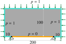
(a)

(b) $C=17.80,\,\texttt{lst}=1$

(c) $C=19.81,\,\texttt{lst}=0$

Figure 14: (14(a)) The design domain, pressure and displacement boundary conditions for the bridge-like structure. In (13(b)) and (13(c)) show the optimized results with lst=1 and lst=0, respectively.

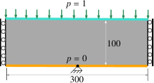
(a)

(b) $C=17.72,\,\texttt{lst}=1$

(c) $C=17.65,\,\texttt{lst}=0$

Figure 15: (15(a)) The piston head the design domain with pressure and displacement boundary conditions. (15(b)) The optimized piston head design with lst=1, (15(c)) The optimized piston head design with lst=0

3.3 Externally pressurized arch structure

The externally pressurized arch problem was first solved in Hammer and Olhoff (2000), and subsequently it also appeared in Chen and Kikuchi (2001); Du and Olhoff (2004); Sigmund and Clausen (2007); Xia et al. (2015); Emmendoerfer Jr et al. (2018); Picelli et al. (2015, 2019); Neofytou et al. (2020), to name a few. The design domain, pressure, and displacement boundary conditions for the problem are shown in Fig. 14(a). The left, right, top, and some parts’ bottom edges are on pressure load $p=1$. Both ends of the bottom edge are fixed, as shown. The following lines of TOPress are modified to account for the boundary conditions associated with this problem. Line 38 (pressure input) is changed to

⬇

PF([Tnode,Lnode,Rnode, Bnode(1:nelx/10), Bnode(end-nelx/10:end)]) = Pin; PF(Bnode(nelx/10+1:end-nelx/10-1)) = 0; % applying pressure

and line 42 is modified to

⬇

fixedUdofs = [2*Bnode(nelx/10+1)-1 2*Bnode(nelx/10+1) 2*Bnode(end-nelx/10-1)-1 2*Bnode(end-nelx/10-1)]; %fixed displ.

The optimized arch structures with lst=1 in Fig. 14(b) and lst=0 in Fig. 14(c) are respectively obtained by the following function call

⬇

TOPress(200,100,0.2,3,4,0.15,8,lst,100)

The optimized design with $\texttt{lst}=1$ has relatively lower-height arch and compliance (Fig. 14(b)) than that obtained with $\texttt{lst}=0$ (Fig. 14(c)). Including load sensitivities within the formulation may certainly affect the optimized shape and topology and thus, the final objective value. The shape of the former resembles one presented in Sigmund and Clausen (2007), whereas the shape of the latter resembles that reported in Picelli et al. (2019); Neofytou et al. (2020).

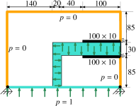
(a)

(b) $C=11.78,\,\texttt{volf}=0.2$

(c) $C=68.52,\,\texttt{volf}=0.4$

Figure 16: (16(a)) The design domain for the pressurized chamber with pressure and displacement boundary conditions. (16(b)) and (16(c)) display the optimized optimized designs with volf $=0.2$ and volf$=0.4$, respectively.

3.4 Piston design

We extend TOPress code for designing the pressure head here. This problem was first reported in Bourdin and Chambolle (2003); after that, many papers also solved it, e.g., Sigmund and Clausen (2007); Picelli et al. (2015); Emmendoerfer Jr et al. (2018); Picelli et al. (2019); Neofytou et al. (2020); Kumar et al. (2020); Huang et al. (2022), to name a few. The design domain specification with pressure and displacement boundary conditions for the piston head model is shown in Fig. 15(a). Pressure load is applied on the top edge, whereas the bottom edge is fixed and set at zero pressure load. The middle point of the bottom edge is fixed. The left and right edges are permitted to move in the $y-$axis. One makes the following changes in TOPress to solve this problem. Line 38 is changed to

⬇

PF(Bnode) = 0; PF(Tnode) = Pin; % applying pressure load

and line 42 is modified to

⬇

fixedUdofs = [2*Bnode(ceil((nelx+1)/2))-1 2*Bnode(ceil((nelx+1)/2)) 2*Lnode-1 2*Rnode-1]; %fixed displ.

The optimized designs depicted in Fig. 15(b), 15(c) that are obtained by the following call

⬇

TOPress(300,100,0.2,3,2.4,0.1,8,lst,150)

with lst=1 and lst=0, respectively.

We consider the full model to solve this problem to check any deviation from the symmetric nature of the problem. One notes that the optimized design retains the symmetric nature (Fig. 15(b)) and qualitatively resembles the features of the piston structures reported in the previous literature. One may also solve this problem using only the symmetric half of the domain. For achieving leak-proof optimized pistons, the user may refer to Kumar et al. (2020) for recommendations on choosing etaf and betaf. Different optimized material layouts are obtained with lst=1 and lst=0.

3.5 Pressurized chamber design

Herein TOPress is modified to solve the pressurized chamber design that was first presented by Hammer and Olhoff (2000). The problem is subsequently solved in Chen and Kikuchi (2001); Zhang et al. (2008); Picelli et al. (2015, 2019); Neofytou et al. (2020); Huang et al. (2022). The design domain with pressure and displacement boundary conditions is shown in Fig. 16(a). The pressure load is applied using a chamber as indicated in the figure. The initial structure of the chamber is constructed through the non-design void and solid regions (Fig. 16). Both corners of the bottom edge and the right most edges of the solid non-design domains are fixed (Fig. 16(a)). The following modifications one needs to perform to solve this problem with TOPress. Lines 34-35 are replaced by

⬇

elNrs = reshape(1:nel,nely,nelx);

sr1 = elNrs(3*nely/8:17*nely/40, 2*nelx/3:nelx);

sr2 = elNrs(23*nely/40:5*nely/8, 2*nelx/3:nelx);

vr1 = elNrs(17*nely/40:end,7*nelx/15:8*nelx/15);

vr2 = elNrs(17*nely/40:23*nely/40,8*nelx/15:nelx);

[NDS, NDV] = deal( [sr1(:);sr2(:)], [vr1(:); vr2(:)] );

act = setdiff( (1 : nel)’, union( NDS, NDV ) );

s1fix = elNrs(3*nely/8:17*nely/40, nelx);

s2fix = elNrs(23*nely/40:25*nely/40, nelx);

fixx = unique(Pdofs([s1fix(:); s2fix(:)],:));

where elNrs gives the matrix of elements for the parameterized domain. sr1 and sr2 provide elements in the solid regions (black bars, Fig. 16(a)). Likewise, vr1 and vr2 record the elements forming void regions. Pressurized regions are also depicted. NDS and NDV contain elements representing solid and void regions, respectively. The rightmost part of the solid regions contain elements recorded in vectors s1fix and s2fix. Vector fixx gives the nodes corresponding to s1fix and s2fix, which are fixed. Next, line 46 is changed to

⬇

PF([Tnode,Lnode,Rnode]) = 0; PF([unique(Pdofs(NDV,:))’,Bnode]) = Pin;% applying pressure load

and line 50 is altered to

⬇

fixedUdofs = [2*Bnode(1)-1 2*Bnode(1) 2*Bnode(end)-1 2*Bnode(end) 2*fixx’-1 2*fixx’]; %fixed displ.

With the above modifications, the code is called as

⬇

TOPress(300,200,volf,3,6,0.1,10,1,200),

The optimized results corresponding to volf=0.2 and volf =0.4 are shown in Fig. 16(b) and Fig. 16(c), respectively. Features of the optimized designs resemble those reported in the previous research papers. The optimized shape of the pressure chamber changes into an arbitrary shape. In addition, the pressure chamber gets a small arch design at the rightmost part of the bottom edge, which is expected in accordance with the boundary conditions of the internally pressurized arch structure (Fig. 8).

3.6 Heaviside projection filter

The 100-line code is extended here with the Heaviside projection filter to achieve the optimized pressure loadbearing designs close to 0-1 . Three variables are used to represent each element: the actual variable ($\rho$), the filtered variable ($\tilde{\rho})$, and the projection variable ($\bar{\rho})$. The latter is determined for element $i$ as

$$\bar{\rho}_{i}=\frac{\tanh(\frac{\beta}{2})+\tanh(\beta(\tilde{\rho}_{i}-\frac{1}{2}))}{2\tanh(\frac{\beta}{2})},$$ (20)

where $\beta\in[0,\,\infty)$ is called the steepness parameter, and $\bar{\rho}_{i}$ is also termed the physical variable of element $i$. We represent $\rho$, $\tilde{\rho}$ and $\bar{\rho}$ by $\mathtt{x}$,  $\mathtt{xtilde}$ and $\mathtt{xPhys}$ in the extended code. Here, $\beta$ is increased from $1$ to $\beta_{\text{max}}=256$ using a continuation scheme wherein $\beta$ gets doubled at every 25 MMA iterations. The chain rule is employed to determine the derivative of $\bar{\rho}$ with respect to $\rho$ and thus that of the objective and constraints. One determines derivatives of $\bar{\rho}$ with respect to $\tilde{\rho}$ as

$$\frac{\partial\bar{\rho}_{i}}{\partial\tilde{{\rho_{i}}}}=\beta\frac{1-\tanh(\beta(\tilde{{\rho_{i}}}-\frac{1}{2}))^{2}}{2\tanh(\frac{\beta}{2})}.$$ (21)

TOPress is modified to cater to this filter for the internally pressurized arch design (Sec. 3.1). One can adopt similar steps for achieving black-and-white loadbearing designs for other problems with the projection filter. The following piece of code is inserted after line 57

⬇

betap = 1;

xPhys = IFprj(xTilde,0.5,betap);

where betap represents $\beta$ (20). Vector xTilde that corresponds to the filtered variables is defined and initialized on line 52. The following line is inserted after line 62 to evaluate the filter matrix dHs as

⬇

dHs = Hs./ reshape( dIFprj( xTilde, 0.5, betap ), nely, nelx);

As the matrix dHs varies in each iteration, the derivatives of volume constraint is now determined within the loop after line 86 as

⬇

dVol = imfilter(reshape(dVol0, nely, nelx)./dHs,h); %filtered volume sensitivity

The objective sensitivities are accordingly determined using dHs. Lines 96-97 are replaced by

⬇

xMMA = xnew; xTilde(act) = xnew;

xTilde = imfilter(reshape(xTilde, nely, nelx),h)./Hs;xTilde = xTilde(:);

if(mod(loop,25)==0 && betap<=betamax), betap= betap*2;end

xphys = IFprj(xTilde,0.5,betap);xphys(NDS)=1; xphys(NDV)=0;

wherein $\beta$ (betap) is doubled at each 25 MMA iterations until it reaches to $\beta_{\text{max}}$ (betamax). The projection filtering and updation of $\beta$ ideally should be performed after line 99 as the employed projection filter is not volume preserving. However, to keep the printing/plotting position consistent and notwithstanding the small error introduced in printing values, we have included projection filtering on line 96-97. We now include $\beta_{\text{max}}$ (betamax) in the input of the main code

⬇

TOPress(nelx,nely,volfrac,penal,rmin,etaf,betaf,betamax,lst,maxit)

One should set an appropriate value for $\beta_{\text{max}}$ so that it can be achieved within the assigned maxit. With the above modification, the code is called with $\texttt{volf}=0.3,\,\texttt{rmin}=4.8,\,\texttt{etaf}=0.2,\,\texttt{betaf}=8,\,\texttt{betamax}=256,\,\texttt{lst}=1$, as

⬇

TOPress(200,100,0.30,3,2.4,0.2,8,256,1,250)

to solve the internally pressurized arch design.

Figure 17: Optimized internally pressurized arch structure with the Heaviside projection. $C=30.39$

Fig. 17 displays the optimized material layout of the internally pressurized arch structure with the Heaviside projection filter. The obtained gray scale parameter $M_{nd}$ (Sigmund, 2007) of the optimized structure is $8.77\text{\times}{10}^{-6}\text{\,}$% which indicates that the optimized arch structure is very close to binary.

Figure 18: Optimized pressure chamber design with the projection filter. $C=61.87$

We also implement the projection filter for the pressure chamber design problem (Sec. 3.5) After incorporating the aforementioned changes, the 100-line code is called with the projection filter for the pressurized chamber with volume fraction 0.4 as

⬇

TOPress(300,200,0.40,3,6,0.1,10,256,1,250)

The optimized design with material layout is depicted in Fig. 18. $M_{\text{nd}}=3.1\times${10}^{-2}\text{\,}$$% is found. Thus, the optimized pressure chamber design (Fig. 18) is close to a 0-1 solution. The topology of the optimized design (Fig. 18) is different than that obtained without the projection filter (Fig. 16(c)). The cardinal reason could be that the projection filter changes the search direction, leading to a different optimum point and, thus, a different optimized topology.

3.7 Other extensions

The numerical experiments performed in the above subsections suggest that TOPress can be readily modified to determine optimized designs for different pressure loadbearing structures. Problems in Figs. 8, 13(a), 14(a) and 15(a) can also be solved by exploiting their vertical symmetric nature, we, however, use the full domain to check any deviation from symmetric. Extending the code for three-dimensional problems requires modifications, though the structure of the code may remain the same. The 100-line code can also be extended to design pressure-driven compliant mechanisms per Kumar et al. (2020); Kumar and Langelaar (2021). Further, toward additional physics, one can develop the code for thermal-fluid problems with design-dependent deformation (Zhao et al., 2021). Furthermore, one can extend the code with advanced constraints, e.g., buckling, stress, etc., as per the requirement.

4 Concluding remarks

This paper presents a compact 100-line MATLAB code, TOPress, for topology optimization of structures involving design-dependent pressure loads using the method of moving asymptotes. Such loads alter their magnitude, direction, and location with topology optimization’s progress; dealing with them becomes a challenging and involved task. TOPress, developed based on the method first proposed in Kumar et al. (2020), aims to facilitate the newcomers’ and students’ learning and provide a potential platform for extending and developing codes/strategies for different applications involving design-dependent pressure loads. The 100-line code and its simple extensions for different problems are explained in detail. A subroutine to plot the pressure field with material layout is also provided. The code is provided in Appendix B. Extending the code for three-dimensional problems requires modification on multiple fronts; however, the structure of the code may remain the same. The code can also be extended for the design problems with advanced constraints, e.g., buckling, stress, etc.

In conjunction with the drainage term, the Darcy law is employed to model the pressure load, wherein the flow coefficient is defined using a smooth Heaviside function per Kumar et al. (2020). The consistent nodal loads corresponding to the obtained pressure field are determined. The approach is qualified using three preliminary numerical examples, which indicate that the Darcy law with the drainage term gives the appropriate (realistic) and accurate pressure load modeling and nodal force calculation. The approach facilitates computationally cheap determination of the load sensitivities, which can be switched on/off in the provided code.

Compliance of the structure is minimized with the given volume fraction. Benchmark problems involving pressure load are solved with and without load sensitivities. Including load sensitivities within the formulation can affect the optimized designs’ shape and topology, and thus the final objective values. One can obtain relatively better-performing pressure loadbearing structures using the load sensitivities. Based on the numerical examples we perform, it is recommended to consider load sensitivities while optimizing such problems; neglecting them cannot be considered physically correct and a welcomed idea. TOPress contains six main parts which are described in detail. We believe the newcomers, students, and researchers will benefit from the provided codes and the paper, and they will extend/use the codes for their research works involving design-dependent pressure (pneumatic) loads.

Replication of results

The 100-line code is explained in detail and provided in Appendix B. In addition, TOPress and its extensions are supplied as supplemental material to reproduce the solutions. If anything is missing can be obtained directly from the author.

Compliance to ethical standards

Conflicts of interest

The author declares no conflicts of interest.

Ethical approval

This article does not contain any studies with human participants or animals performed by the author.

Appendix A Expressions for flow and transformation matrices: $\mathbf{\mathbf{K}}_{\text{p}}^{i}$, $\mathbf{K}^{i}_{\text{Dp}}$ and $\mathbf{T}_{i}$

The expressions for the flow matrices $\mathbf{\mathbf{K}}_{\text{p}}^{i}$ and $\mathbf{K}^{i}_{\text{Dp}}$, and transformation matrix $\mathbf{T}_{i}$ are provided for element $i$ herein.

Figure 19 displays the local node numbers with nodal coordinates $(x_{i},\,y_{i})$, $(x_{i}+\text{D}x,\,y_{i})$, $(x_{i}+\text{D}x,\,y_{i}+\text{D}y)$, and $(x_{i},\,y_{i}+\text{D}y)$ for element $i$ .

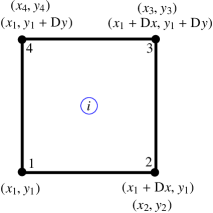
Figure 19: Nodal coordinates of element $i$

As mentioned earlier, we employ the bi-linear shape functions for the finite element analysis. To determine, $\mathbf{\mathbf{K}}_{\text{p}}^{i}$ and $\mathbf{K}^{i}_{\text{Dp}}$ as written in (5) and $\mathbf{T}_{i}$ as provided in (9), numerical integration approach using the Gauss points is employed (Zienkiewicz et al., 2005). Mathematically,

$$\mathbf{\mathbf{K}}_{\text{p}}^{i} =\int_{\Omega_{e}}K~{}\mathbf{B}^{\top}_{\text{p}}\mathbf{B}_{\text{p}}\text{d}V$$ (A.1)

$$=t_{i}\int_{-1}^{1}\int_{-1}^{1}\left(K~{}\mathbf{B}^{\top}_{\text{p}}\mathbf{B}_{\text{p}}\right)\det\mathbf{J}d\xi d\zeta$$

$$\mathbf{K}^{i}_{\text{Dp}} =\int_{\Omega_{e}}D~{}\mathbf{N}^{\top}_{\text{p}}\mathbf{N}_{\text{p}}\text{d}V$$

$$=t_{i}\int_{-1}^{1}\int_{-1}^{1}\left(D~{}\mathbf{N}^{\top}_{\text{p}}\mathbf{N}_{\text{p}}\right)\det\mathbf{J}d\xi d\zeta$$

$$\mathbf{T}_{i} =-\int_{\mathrm{\Omega}_{e}}{\mathbf{N}}^{\!\top}_{\mathbf{u}}\mathbf{B}_{\text{p}}\text{d}V=t_{i}\int_{-1}^{1}\int_{-1}^{1}{\mathbf{N}}^{\!\top}_{\mathbf{u}}\mathbf{B}_{\text{p}}\det\mathbf{J}d\xi d\zeta$$

where $\mathbf{J}$ is the Jacobian matrix given as

$$\mathbf{J}=\frac{1}{4}\begin{bmatrix}J11&\quad J12\\ J21&\quad J22,\end{bmatrix}$$ (A.2)

where $J11=-(1-\zeta)x_{1}+(1-\zeta)x_{2}+(1+\zeta)x_{3}-(1+\zeta)x_{4}$, $J12=\quad-(1-\zeta)y_{1}+(1-\zeta)y_{2}+(1+\zeta)y_{3}-(1+\zeta)y_{4}$, $J21=-(1-\xi)x_{1}+(1-\xi)x_{2}+(1+\xi)x_{3}-(1+\xi)x_{4},$ and $J22=-(1-\xi)y_{1}+(1-\xi)y_{2}+(1+\xi)y_{3}-(1+\xi)y_{4}$, with $N_{k}=\frac{1}{4}(1+\xi\xi_{k})(1+\zeta\zeta_{k})$, where $(\xi_{k},\,\zeta_{k})$ are natural coordinates with (-1, -1), (1, -1), (1, 1) and (-1, 1) for node $k$. (A.1) yields the following with $2\times 2$ Gauss-quadrature rule:

$$\mathbf{\mathbf{K}}_{\text{p}}^{i}=\frac{t_{i}}{6DxDy}\begin{bmatrix}K_{p1}&\quad K_{p2}&\quad-0.5K_{p1}&\quad K_{p3}\\ &\quad K_{p1}&\quad K_{p3}&\quad-0.5K_{p1}\\ &\text{Sym.}&K_{p1}&\quad K_{p2}\\ &&&\quad K_{p1}\end{bmatrix}$$ (A.3)

where $K_{p1}=2(Dx^{2}+Dy^{2})$,  $K_{p2}=Dx^{2}-2Dy^{2}$, $K_{p3}=Dy^{2}-2Dx^{2}$.

$$\mathbf{\mathbf{K}}_{\text{Dp}}^{i}=\frac{t_{i}DxDy}{36}\begin{bmatrix}4&\quad 2&\quad 1&\quad 2\\ &\quad 4&\quad 2&\quad 1\\ &\text{Sym.}&\quad 4&\quad 2\\ &&&\quad 4\end{bmatrix}$$ (A.4)

and

$$\mathbf{T}_{i}=\frac{t_{i}}{12}\begin{bmatrix}-2Dy&\quad 2Dy&\quad Dy&\quad-Dy\\ -2Dx&\quad-Dx&\quad Dx&\quad 2Dx\\ -2Dy&\quad 2Dy&\quad Dy&\quad-Dy\\ -Dx&\quad-2Dx&\quad 2Dx&\quad Dx\\ -Dy&\quad Dy&\quad 2Dy&\quad-2Dy\\ -Dx&\quad-2Dx&\quad 2Dx&\quad Dx\\ -Dy&\quad Dy&\quad 2Dy&\quad-2Dy\\ -2Dx&\quad-Dx&\quad Dx&\quad 2Dx\end{bmatrix}$$ (A.5)

For the square elements which we consider to parameterize the design domain with $t_{i}=1$ (plane-stress cases). The expressions for $\mathbf{\mathbf{K}}_{\text{p}}^{i}$, $\mathbf{\mathbf{K}}_{\text{Dp}}^{i}$ and $\mathbf{T}_{i}$ transpire to

$$\mathbf{\mathbf{K}}_{\text{p}}^{i}=\frac{1}{6}\begin{bmatrix}4&\quad-1&\quad-2&\quad-1\\ &4&\quad-1&\quad-2\\ &\text{Sym.}&4&\quad-1\\ &&&4\end{bmatrix}$$ (A.6)

$$\mathbf{\mathbf{K}}_{\text{Dp}}^{i}=\frac{1}{36}\begin{bmatrix}4&\quad 2&\quad 1&\quad 2\\ &\quad 4&\quad 2&\quad 1\\ &\text{Sym.}&\quad 4&\quad 2\\ &&&\quad 4\end{bmatrix}$$ (A.7)

and

$$\mathbf{T}_{i}=\frac{1}{12}\begin{bmatrix}-2&\quad 2&\quad 1&\quad-1\\ -2&\quad-1&\quad 1&\quad 2\\ -2&\quad 2&\quad 1&\quad-1\\ -1&\quad-2&\quad 2&\quad 1\\ -1&\quad 1&\quad 2&\quad-2\\ -1&\quad-2&\quad 2&\quad 1\\ -1&\quad 1&\quad 2&\quad-2\\ -2&\quad-1&\quad 1&\quad 2\end{bmatrix}$$ (A.8)

Appendix B The MATLAB code: TOPress

⬇

1function TOPress(nelx,nely,volfrac,penal,rmin,etaf,betaf,lst,maxit)

2%% ___PART 1.____________________________MATERIAL AND FLOW PARAMETERS

3E1 = 1;

4Emin = E1*1e-6;

5nu = 0.30;

6[Kv,epsf,r,Dels] = deal(1,1e-7,0.1,2); % flow parameters

7[Ds, kvs]= deal((log(r)/Dels)^2*epsf,Kv*(1 - epsf)); % flow parameters

8%% ____PART 2._______________FINITE ELEMENT ANALYSIS PREPARATION and NON-DESIGN DOMAIN

9[nel,nno] = deal(nelx*nely, (nelx+1)*(nely+1));

10nodenrs = reshape(1:(1+nelx)*(1+nely),1+nely,1+nelx);

11edofVec = reshape(2*nodenrs(1:end-1,1:end-1)+1,nelx*nely,1);

12Udofs = repmat(edofVec,1,8)+repmat([0 1 2*nely+[2 3 0 1] -2 -1],nelx*nely,1);

13[Lnode,Rnode,]= deal(1:nely+1, (nno-nely):nno);

14[Bnode,Tnode]= deal((nely+1):(nely+1):nno, 1:(nely+1):(nno-nely));

15[Pdofs,allPdofs, allUdofs] = deal(Udofs(:,2:2:end)/2,1:nno,1:2*nno);

16iP = reshape(kron(Pdofs,ones(4,1))’,16*nel,1);

17jP = reshape(kron(Pdofs,ones(1,4))’,16*nel,1);

18iT = reshape(kron(Udofs,ones(4,1))’,32*nel,1);

19jT = reshape(kron(Pdofs,ones(1,8))’,32*nel,1);

20iK = reshape(kron(Udofs,ones(8,1))’,64*nel,1);

21jK = reshape(kron(Udofs,ones(1,8))’,64*nel,1);

22Kp = 1/6*[4 -1 -2 -1;-1 4 -1 -2; -2 -1 4 -1; -1 -2 -1 4]; % flow matrix: Darcy Law

23KDp = 1/36*[4 2 1 2; 2 4 2 1; 1 2 4 2; 2 1 2 4]; % Drainage matrix

24Te = 1/12*[-2 2 1 -1;-2 -1 1 2;-2 2 1 -1;-1 -2 2 1;-1 1 2 -2; -1 -2 2 1; -1 1 2 -2; -2 -1 1 2]; % tran matrix

25A11 = [12 3 -6 -3; 3 12 3 0; -6 3 12 -3; -3 0 -3 12];

26A12 = [-6 -3 0 3; -3 -6 -3 -6; 0 -3 -6 3; 3 -6 3 -6];

27B11 = [-4 3 -2 9; 3 -4 -9 4; -2 -9 -4 -3; 9 4 -3 -4];

28B12 = [ 2 -3 4 -9; -3 2 9 -2; 4 9 2 3; -9 -2 3 2];

29ke = 1/(1-nu^2)/24*([A11 A12;A12’ A11]+nu*[B11 B12;B12’ B11]); %stiffness matrix

30IFprj=@(xv,etaf,betaf)((tanh(betaf*etaf) + tanh(betaf*(xv-etaf)))/... %projection function

31 (tanh(betaf*etaf) + tanh(betaf*(1 - etaf))));

32dIFprj=@(xv,etaf,betaf) betaf*(1-tanh(betaf*(xv-etaf)).^2)...

33 /(tanh(betaf*etaf)+tanh(betaf*(1-etaf))); % derivative of the projection function

34[NDS, NDV ] = deal( [], [] );

35act = setdiff((1 : nel)’, union( NDS, NDV ));

36%% ____PART 3.______PRESSURE & STRUCTURE B.C’s, LOADs

37[PF, Pin] =deal(0.00001*ones(nno,1),1); %pressure-field preparation

38PF([Tnode,Lnode,Rnode]) = 0; PF(Bnode) = Pin; % applying pressure load

39fixedPdofs = allPdofs(PF~=0.00001); % given P-dofs

40freePdofs = setdiff(allPdofs,fixedPdofs); % free P-dofs

41pfixeddofsv = [fixedPdofs’ PF(fixedPdofs)]; % p-fixed and its value

42fixedUdofs = [2*Bnode(1)-1 2*Bnode(1) 2*Bnode(end)-1 2*Bnode(end)]; %fixed displ.

43freeUdofs = setdiff(allUdofs,fixedUdofs); % free dofs for displ.

44[U, lam1] = deal(zeros(2*nno,1),zeros(nno,1)); %lam1:Lagrange mult.

45%% ___PART 4._________________________________________FILTER PREPARATION

46[dy,dx] = meshgrid(-ceil(rmin)+1:ceil(rmin)-1,-ceil(rmin)+1:ceil(rmin)-1);

47h = max( 0, rmin-sqrt( dx.^2 + dy.^2 ) ); % conv. kernel

48Hs = imfilter(ones(nely, nelx ), h); % matrix of weights (filter)

49%% ___PART 5.__________________________MMA OPTIMIZATION PREPARATION & INITIALIZATION

50[x,dVol0] = deal(zeros(nel,1),ones(nel,1)/(nel*volfrac)); %design var. and vol. cont. der.

51x(act) = (volfrac*(nel-length(NDV))-length(NDS) )/length(act); x(NDS) = 1; % updating

52[nMMA,mMMA,xphys,xMMA,mvLt] = deal(length(act),1,x,x(act),0.1); % diff. varbls.

53[xminvec,xmaxvec] = deal(zeros(nMMA,1),ones(nMMA,1)); %Min. & Max

54[low, upp] = deal(xminvec,xmaxvec); % Low and Upp limits MMA

55[cMMA,dMMA, a0, aMMA] = deal(1000*ones(mMMA,1),zeros(mMMA,1),1,zeros(mMMA,1));

56[xold1,xold2] = deal(xMMA);

57[loop, change] =deal(0,1); % loop counter and convergence change criteria

58dVol = imfilter(reshape(dVol0, nely, nelx)./Hs,h); %filtered volume sensitivity

59%% ____PART 6._____________________________________MMA OPTIMIZATION LOOP

60while(loop<maxit && change>0.01)

61loop = loop + 1; % Updating the opt. iteration

62%___PART 6.1__________SOLVING FLOW BALANCE EQUATION

63Kc = Kv*(1-(1-epsf)*IFprj(xphys,etaf,betaf)); %Flow coefficient

64Dc = Ds*IFprj(xphys,etaf,betaf); %Drainage coefficient

65Ae = reshape(Kp(:)*Kc’ + KDp(:)*Dc’,16*nel,1); %Elemental flow matrix

66AG = (sparse(iP,jP,Ae)+ sparse(iP,jP,Ae)’)/2; %Global flow matrix

67Aff = AG(freePdofs,freePdofs); %AG for free pressure dofs

68PF(freePdofs) = decomposition(Aff,’ldl’)\(-AG(freePdofs,fixedPdofs)*pfixeddofsv(:,2));

69PF(pfixeddofsv(:,1)) = pfixeddofsv(:,2); % Final P-field

70%__PART 6.2_DETERMINING CONSISTENT NODAL LOADS and GLOBAL Disp. Vector

71Ts = reshape(Te(:)*ones(1,nel), 32*nel, 1); %Elemental transformation matrix

72TG = sparse(iT, jT, Ts); %Global transformation matrix

73F = -TG*PF; % Dertmining nodal forces

74E = Emin + xphys.^penal*(E1 - Emin); %Material interpolation

75Ks = reshape(ke(:)*E’,64*nel,1); %Elemental stiffness matrix

76KG = (sparse(iK,jK,Ks) + sparse(iK,jK,Ks)’)/2; %Global stiffnes matrix

77U(freeUdofs) = decomposition(KG(freeUdofs,freeUdofs),’chol’,’lower’)\F(freeUdofs); %Global Disp. Vect.

78%__PART 6.3__OBJECTIVE, CONSTRAINT and THEIR SENSITIVITIES COMPUTATION

79obj = U’*KG*U; % determining objective

80lam1(freePdofs) = (2*U(freeUdofs)’*TG(freeUdofs,freePdofs))/Aff; % Lagrange mult.

81objsT1 = -(E1 - Emin)*penal*xphys.^(penal - 1).*sum(([U(Udofs)]*ke).*[U(Udofs)],2);

82dC1k = -dIFprj(xphys,etaf,betaf).* sum((lam1(Pdofs)*(kvs*Kp)) .* PF(Pdofs),2);

83dC1h = dIFprj(xphys,etaf,betaf).* sum((lam1(Pdofs)*(Ds*KDp)) .* PF(Pdofs),2);

84objsT2 = dC1k + dC1h; objsens = (objsT1 + lst*objsT2); % final sensitivities

85Vol = sum(xphys)/(nel*volfrac)-1; % volume fraction

86if(loop ==1), normf = 1000/(obj);save normf normf;end, load normf normf;

87objsens = imfilter(reshape(objsens*normf, nely, nelx)./Hs,h); % Obj. sens.

88%___PART 6.4______________________SETTING and CALLING MMA OPTIMIZATION

89xval = xMMA;

90[xminvec, xmaxvec]= deal(max(0, xval - mvLt),min(1, xval + mvLt));

91[xmma,~,~,~,~,~,~,~,~,low,upp] = mmasub(mMMA,nMMA,loop,xval,xminvec,xmaxvec,xold1,xold2, ...

92 obj*normf,objsens(act)’,objsens(act)’*0,Vol,dVol(act)’,dVol(act)’*0,low,upp,a0,aMMA,cMMA,dMMA); % call MMA

93[xold2,xold1, xnew]= deal(xold1, xval,xmma); % updating

94change = max(abs(xnew-xMMA)); % Calculating change

95xMMA = xnew; xphys(act) = xnew;xphys = imfilter(reshape(xphys, nely, nelx),h)./Hs;

96xphys = xphys(:); xphys(NDS)=1; xphys(NDV)=0; % updating xphys

97%___PART 6.5_____________________________Printing and plotting results

98fprintf(’ It.:%5i Obj.:%11.4f Vol.:%7.3f ch.:%7.3f\n’,loop,obj*normf,mean(xphys),change);

99colormap(gray); imagesc(1-reshape(xphys, nely, nelx));caxis([0 1]);axis equal off;drawnow;

100end

numbers=none

⬇

1%%%%%%%%%%%%%%%%%%%%%%%%%%%%%%%%%%%%%%%%%%%%%%%%%%%%%%%%%%%%%%%%%%%%%%%%%%%%%%%%%%%%%%

2% The code, TOPress, is provided for pedagogical purposes. A detailed %

3% description is presented in the paper:"TOPress: a MATLAB implementation for %

4% topology optimization of structures subjected to design-dependent pressure %

5% loads" Structural and Mutltidisciplinary Optimization, 2023. %

6% %

7% One can download the code and its extensions for the different problems %

8% from the online supplementary material and also from: %

9% https://github.com/PrabhatIn/TOPress %

10% %

11% Please send your comment to: pkumar@mae.iith.ac.in %

12% %

13% One may also refer to the following two papers for more detail: %

14% %

15% 1. Kumar P, Frouws JS, Langelaar M (2020) Topology optimization of fluidic %

16% pressure-loaded structures and compliant mechanisms using the Darcy method. %

17% Structural and Multidisciplinary Optimization 61(4):1637-1655 %

18% 2. Kumar P, Langelaar M (2021) On topology optimization of design-dependent %

19% pressure-loaded three-dimensional structures and compliant mechanisms. %

20% International Journal for Numerical Methods in Engineering 122(9):2205-2220 %

21% %

22% Disclaimer: %

23% The author does not guarantee that the code is free from erros but reserves %

24% all rights. Further, the author shall not be liable in any event caused by %

25% use of the above 100-line code and its extensions %

26% %

27%%%%%%%%%%%%%%%%%%%%%%%%%%%%%%%%%%%%%%%%%%%%%%%%%%%%%%%%%%%%%%%%%%%%%%%%%%%%%%%%%%%%%%

References

- Ali and Shimoda (2022) Ali MA, Shimoda M (2022) Toward multiphysics multiscale concurrent topology optimization for lightweight structures with high heat conductivity and high stiffness using MATLAB. Structural and Multidisciplinary Optimization 65(7):1–26
- Andreassen and Andreasen (2014) Andreassen E, Andreasen CS (2014) How to determine composite material properties using numerical homogenization. Computational Materials Science 83:488–495
- Andreassen et al. (2011) Andreassen E, Clausen A, Schevenels M, Lazarov BS, Sigmund O (2011) Efficient topology optimization in MATLAB using 88 lines of code. Structural and Multidisciplinary Optimization 43(1):1–16
- Bourdin and Chambolle (2003) Bourdin B, Chambolle A (2003) Design-dependent loads in topology optimization. ESAIM: Control, Optimisation and Calculus of Variations 9:19–48
- Bruns and Tortorelli (2001) Bruns TE, Tortorelli DA (2001) Topology optimization of non-linear elastic structures and compliant mechanisms. Comput Method Appl Mech Eng 190(26-27):3443–3459
- Bruyneel and Duysinx (2005) Bruyneel M, Duysinx P (2005) Note on topology optimization of continuum structures including self-weight. Structural and Multidisciplinary Optimization 29(4):245–256
- Chen and Kikuchi (2001) Chen BC, Kikuchi N (2001) Topology optimization with design-dependent loads. Finite elements in analysis and design 37(1):57–70
- Christiansen and Sigmund (2021) Christiansen RE, Sigmund O (2021) Compact 200 line MATLAB code for inverse design in photonics by topology optimization: tutorial. JOSA B 38(2):510–520
- Du and Olhoff (2004) Du J, Olhoff N (2004) Topological optimization of continuum structures with design-dependent surface loading–part i: new computational approach for 2D problems. Structural and Multidisciplinary Optimization 27(3):151–165
- Emmendoerfer Jr et al. (2018) Emmendoerfer Jr H, Fancello EA, Silva ECN (2018) Level set topology optimization for design-dependent pressure load problems. International Journal for Numerical Methods in Engineering 115(7):825–848
- Ferrari et al. (2021) Ferrari F, Sigmund O, Guest JK (2021) Topology optimization with linearized buckling criteria in 250 lines of matlab. Structural and Multidisciplinary Optimization 63(6):3045–3066
- Gao et al. (2019) Gao J, Luo Z, Xia L, Gao L (2019) Concurrent topology optimization of multiscale composite structures in matlab. Structural and Multidisciplinary Optimization 60(6):2621–2651
- Hammer and Olhoff (2000) Hammer VB, Olhoff N (2000) Topology optimization of continuum structures subjected to pressure loading. Structural and Multidisciplinary Optimization 19(2):85–92
- Han et al. (2021) Han Y, Xu B, Liu Y (2021) An efficient 137-line MATLAB code for geometrically nonlinear topology optimization using bi-directional evolutionary structural optimization method. Structural and Multidisciplinary Optimization 63(5):2571–2588
- Huang et al. (2022) Huang H, Hu J, Liu S, Liu Y (2022) A thermal-solid–fluid method for topology optimization of structures with design-dependent pressure load. Acta Mechanica Solida Sinica pp 1–12
- Ibhadode et al. (2020) Ibhadode O, Zhang Z, Rahnama P, Bonakdar A, Toyserkani E (2020) Topology optimization of structures under design-dependent pressure loads by a boundary identification-load evolution (bile) model. Structural and Multidisciplinary Optimization 62(4):1865–1883
- Kumar (2023) Kumar P (2023) HoneyTop90: A 90-line MATLAB code for topology optimization using honeycomb tessellation. Optimization and Engineering 24(2):1433-1460
- Kumar (2022) Kumar P (2022) Topology optimization of stiff structures under self-weight for given volume using a smooth Heaviside function. Structural and Multidisciplinary Optimization 65(4):1–17
- Kumar (2023) Kumar P (2023) Towards Topology Optimization of Pressure-Driven Soft Robots. In: Conference on Microactuators and Micromechanisms, Springer, pp 19–30
- Kumar and Langelaar (2021) Kumar P, Langelaar M (2021) On topology optimization of design-dependent pressure-loaded three-dimensional structures and compliant mechanisms. International Journal for Numerical Methods in Engineering 122(9):2205–2220
- Kumar et al. (2020) Kumar P, Frouws JS, Langelaar M (2020) Topology optimization of fluidic pressure-loaded structures and compliant mechanisms using the Darcy method. Structural and Multidisciplinary Optimization 61(4):1637–1655
- Neofytou et al. (2020) Neofytou A, Picelli R, Huang TH, Chen JS, Kim HA (2020) Level set topology optimization for design-dependent pressure loads using the reproducing kernel particle method. Structural and Multidisciplinary Optimization 61(5):1805–1820
- Picelli et al. (2015) Picelli R, Vicente W, Pavanello R (2015) Bi-directional evolutionary structural optimization for design-dependent fluid pressure loading problems. Engineering Optimization 47(10):1324–1342
- Picelli et al. (2019) Picelli R, Neofytou A, Kim HA (2019) Topology optimization for design-dependent hydrostatic pressure loading via the level-set method. Structural and Multidisciplinary Optimization 60(4):1313–1326
- Saxena (2011) Saxena A (2011) Topology design with negative masks using gradient search. Structural and Multidisciplinary Optimization 44(5):629–649
- Sigmund (2001) Sigmund O (2001) A 99 line topology optimization code written in matlab. Structural and multidisciplinary optimization 21(2):120–127
- Sigmund (2007) Sigmund O (2007) Morphology-based black and white filters for topology optimization. Struct Multidiscip O 33(4-5):401–424
- Sigmund and Clausen (2007) Sigmund O, Clausen PM (2007) Topology optimization using a mixed formulation: an alternative way to solve pressure load problems. Computer Methods in Applied Mechanics and Engineering 196(13-16):1874–1889
- Sigmund and Maute (2013) Sigmund O, Maute K (2013) Topology optimization approaches. Structural and Multidisciplinary Optimization 48(6):1031–1055
- Svanberg (1987) Svanberg K (1987) The method of moving asymptotes–a new method for structural optimization. Int J Numer Meth Eng 24(2):359–373
- Talischi et al. (2012) Talischi C, Paulino GH, Pereira A, Menezes IF (2012) PolyTop: a matlab implementation of a general topology optimization framework using unstructured polygonal finite element meshes. Structural and Multidisciplinary Optimization 45(3):329–357
- Wang et al. (2021) Wang C, Zhao Z, Zhou M, Sigmund O, Zhang XS (2021) A comprehensive review of educational articles on structural and multidisciplinary optimization. Structural and Multidisciplinary Optimization 64(5):2827–2880
- Xavier et al. (2022) Xavier MS, Tawk CD, Zolfagharian A, Pinskier J, Howard D, Young T, Lai J, Harrison SM, Yong YK, Bodaghi M, et al. (2022) Soft pneumatic actuators: A review of design, fabrication, modeling, sensing, control and applications. IEEE Access
- Xia and Breitkopf (2015) Xia L, Breitkopf P (2015) Design of materials using topology optimization and energy-based homogenization approach in Matlab. Structural and multidisciplinary optimization 52(6):1229–1241
- Xia et al. (2015) Xia Q, Wang MY, Shi T (2015) Topology optimization with pressure load through a level set method. Computer Methods in Applied Mechanics and Engineering 283:177–195
- Zhang et al. (2008) Zhang H, Zhang X, Liu S (2008) A new boundary search scheme for topology optimization of continuum structures with design-dependent loads. Structural and Multidisciplinary Optimization 37(2):121–129
- Zhao et al. (2021) Zhao J, Zhang M, Zhu Y, Cheng R, Wang L, Li X (2021) Topology optimization of planar heat sinks considering out-of-plane design-dependent deformation problems. Meccanica 56(7):1693–1706
- Zienkiewicz et al. (2005) Zienkiewicz OC, Taylor RL, Zhu JZ (2005) The finite element method: its basis and fundamentals. Elsevier