Controllability and Stabilizability of the linearized compressible Navier-Stokes system with Maxwell’s law

Abstract.

In this paper, we study the control properties of the linearized compressible Navier-Stokes system with Maxwell’s law around a constant steady state $(\rho_{s},u_{s},0),\rho_{s}>0,u_{s}>0$ in the interval $(0,2\pi)$ with periodic boundary data. We explore the exact controllability of the coupled system by means of a localized interior control acting in any of the equations when time is large enough. We also study the boundary exact controllability of the linearized system using a single control force when the time is sufficiently large. In both cases, we prove the exact controllability of the system in the space $L^{2}(0,2\pi)\times L^{2}(0,2\pi)\times L^{2}(0,2\pi)$. We establish the exact controllability results by proving an observability inequality with the help of an Ingham-type inequality. Next, we prove the small time lack of controllability of the concerned system for the case of localized interior control.

Further, using a Gramian-based approach demonstrated by Urquiza, we prove the exponential stabilizability of the corresponding closed-loop system with an arbitrary prescribed decay rate using boundary feedback control law.

1. Introduction and Main results

1.1. Setting of the problem

The control and stabilization of fluid flow have been extensively studied due to their numerous practical applications such as weather prediction, water flow in a pipe, designing aircraft and cars. Many researchers have been interested in the subject of the controllability of fluid flows, more so for incompressible flow (see [2], [19], [33], [34], [37]) than for compressible flow (see [11], [12]). In our research, we focus on investigating the exact controllability and stabilizability of the linearized compressible Navier-Stokes system with Maxwell’s law.

Let us consider the one-dimensional compressible Navier-Stokes system in the domain $(0,2\pi)$:

$$\left.\begin{aligned} &\partial_{t}\hat{\rho}+\partial_{x}(\hat{\rho}\hat{u})=0\qquad\qquad\qquad\qquad\text{ in }(0,T)\times(0,2\pi),\\ &\partial_{t}\left({\hat{\rho}\hat{u}}\right)+\partial_{x}\left({\hat{\rho}\hat{u}^{2}}\right)+\partial_{x}p=\partial_{x}\hat{S}\qquad\text{in }(0,T)\times(0,2\pi),\end{aligned}\right\}$$ (1.1)

where, $\hat{\rho}$, $\hat{u}$, $p$ and $\hat{S}$ represent the density, velocity, pressure and stress tensor of the fluid, respectively. Equation (1.1)₁ is the consequence of conservation of mass and equation (1.1)₂ is the consequence of conservation of momentum. We assume that the pressure $p$ satisfies the following constitutive law:

$$p(\hat{\rho})=a\hat{\rho}^{\gamma},\>\quad\gamma\geq 1,$$ (1.2)

where $a$ is a positive constant. While, the stress tensor $\hat{S}$ is assumed to satisfy the Maxwell’s law:

$$\kappa\partial_{t}\hat{S}+\hat{S}=\mu\partial_{x}\hat{u},\text{ in }(0,T)\times(0,2\pi).$$ (1.3)

Here $\mu$ and $\kappa$ are positive constants, with $\mu$ representing the fluid viscosity and $\kappa$ denoting the relaxation time that characterizes the time delay in the response of the stress tensor to the velocity gradient. For more detailed information, refer to [22] and references therein. Relation $\eqref{max law}$ is first proposed by Maxwell, in order to describe the relation of stress tensor and velocity gradient for a non-simple fluid.

In this paper, we study the control aspects of the one-dimensional compressible Navier-Stokes system with Maxwell’s law and with periodic boundary conditions linearized around a constant steady state $\left(\rho_{s},u_{s},0\right),\rho_{s}>0,u_{s}>0$ of (1.1). More precisely we consider the following system:

$$\left.\begin{aligned} &\partial_{t}\rho+u_{s}\partial_{x}\rho+\rho_{s}\partial_{x}u=\mathbbm{1}_{\mathcal{O}_{1}}f_{1},\qquad&&\text{in }(0,T)\times(0,2\pi),\\ &\partial_{t}u+u_{s}\partial_{x}u+a\gamma{\rho_{s}}^{\gamma-2}\partial_{x}\rho-\frac{1}{\rho_{s}}\partial_{x}S=\mathbbm{1}_{\mathcal{O}_{2}}f_{2},\qquad&&\text{in }(0,T)\times(0,2\pi),\\ &\partial_{t}S+\frac{1}{\kappa}S-\frac{\mu}{\kappa}\partial_{x}u=\mathbbm{1}_{\mathcal{O}_{3}}f_{3},\qquad&&\text{in }(0,T)\times(0,2\pi),\\ &\rho(t,0)=\rho(t,2\pi),\>u(t,0)=u(t,2\pi),\>S(t,0)=S(t,2\pi),\qquad&&t\in(0,T),\\ &\rho(0,x)=\rho_{0}(x),\quad u(0,x)=u_{0}(x),\quad S(0,x)=S_{0}(x),\qquad&&x\in(0,2\pi),\end{aligned}\right\}$$ (1.4)

where $\mathbbm{1_{\mathcal{O}_{j}}}$ is the characteristic function of an open set ${\mathcal{O}}_{j}\subset(0,2\pi),$ $j=1,2,3$ and $f_{i}$, $i=1,2,3$ are the distributed controls.

To establish the controllability results, we have to consider the following restriction on the constant steady state $(\rho_{s},u_{s},0)$:

$$\left(a\gamma\rho_{s}^{\gamma-1}-u_{s}^{2}\right)\geq 0.$$ (1.5)

Definition 1.1.

The system (1.4) is exactly controllable in $(L^{2}(0,2\pi))^{3}$ at time $T>0$, if for any initial condition $(\rho_{0},u_{0},S_{0})^{\top}\in(L^{2}(0,2\pi))^{3}$ and any other $(\rho_{1},u_{1},S_{1})^{\top}\in(L^{2}(0,2\pi))^{3}$, there exist controls $f_{i}\in L^{2}\left(0,T;L^{2}(\mathcal{O}_{i})\right),i=1,2,3,$ such that the corresponding solution $(\rho,u,S)^{\top}$ of (1.4) satisfies

$$(\rho,u,S)^{\top}(T,x)=(\rho_{1},u_{1},S_{1})^{\top}(x),\text{ for all }x\in(0,2\pi).$$ (1.6)

Let us first mention controllability results for some fluid models related to our system. The existence of the solution of the compressible Navier-Stokes system with Maxwell’s law, along with the blow-up results has been studied, for example, in [21, 22, 41] and references therein. If $\kappa=0$, then the Maxwell’s law (1.3) turns into the Newtonian law $\hat{S}=\mu\partial_{x}\hat{u}$ and the equation (1.1) becomes Navier-Stokes system of a viscous, compressible, isothermal barotropic fluid (density is function of pressure only), in a bounded domain $(0,2\pi)$. The compressible Navier-Stokes system linearized around a constant trajectory $(\rho_{s},u_{s})$ for $\rho_{s}>0,u_{s}>0$, yields a coupled transport-parabolic system with constant coefficients. The controllability of such systems with constant coefficients in one dimension has been extensively studied in the literature. In [9, 10], the authors studied this system in the domain $(0,2\pi)$ with periodic boundary conditions and localized interior control acting only in the parabolic equation. In [9], using the moment method, the authors proved the null controllability in $H^{s+1}_{\textnormal{m}}(0,2\pi)\times H^{s}(0,2\pi),$ $s>6.5,$ at time $T>\frac{2\pi}{|u_{s}|},$ where $H^{s}_{\textnormal{m}}(0,2\pi)$ is the space of periodic Sobolev space with mean zero. This result was improved in [10] by showing that the null controllability holds for any initial data in $H^{1}_{\textnormal{m}}(0,2\pi)\times L^{2}(0,2\pi).$ Moreover, the authors also proved that, the system in consideration is not null controllable in $H^{s}_{\textnormal{m}}(0,2\pi)\times L^{2}(0,2\pi),$ $0\leqslant s<1,$ at any time $T>0$ by $L^{2}$-control acting in the parabolic equation. Thus $H^{1}_{\textnormal{m}}(0,2\pi)\times L^{2}(0,2\pi)$ is the largest space in which the system is null controllable by a $L^{2}$-parabolic control.

Recently, in [3], the above results have been extended to more general coupled transport-parabolic systems with constant coefficients. The authors considered coupling of several transport and parabolic equations in one-dimensional torus $\mathbb{T}$ and studied the null controllability with localized interior control in optimal time. Moreover, an algebraic necessary and sufficient condition on the coupling term was obtained when controls act only on the parabolic or transport components. For the extension of these results to the general coupling matrix, one can refer to the work [24].

The local null controllability of the nonlinear compressible Navier-Stokes system around a trajectory with non-zero velocity at large time $T>0$ has been obtained in [16, 15, 17, 31, 30, 32].

In [1], the authors considered the one-dimensional compressible Navier-Stokes equations with Maxwell’s law linearized around a constant steady state $(\rho_{s},0,0),\rho_{s}>0$ with Dirichlet boundary conditions and with interior controls in the interval $(0,\pi)$. They have proved that the system is not null controllable at any time using localized controls in density and stress equations and even everywhere control in the velocity equation. Moreover, they have shown that the system is null controllable at any time $T>0$ in the space $(L^{2}(0,\pi))^{3}$, if the control acts everywhere in the density or stress equation. Approximate controllability at large time using localized controls has also been studied.

In the following subsection, we state our main results regarding the interior controllability of the system (1.4)

1.2. Interior controllability

At first, we consider the case when $f_{2}=0=f_{3}$ in (1.4). Performing integration by parts and using the boundary conditions, from the system (1.4), we deduce

$$\frac{d}{dt}\left(\int_{0}^{2\pi}u(t,x)\>{\rm d}x\right)=0,\quad\frac{d}{dt}\left(\int_{0}^{2\pi}S(t,x)e^{\frac{t}{\kappa}}\>{\rm d}x\right)=0,$$

and therefore,

$$\int_{0}^{2\pi}u(T,x)\>{\rm d}x=\int_{0}^{2\pi}u_{0}(x)\>{\rm d}x,\quad\int_{0}^{2\pi}S(T,x)e^{\frac{T}{\kappa}}\>{\rm d}x=\int_{0}^{2\pi}S_{0}(x)\>{\rm d}x.$$

Thus if the system (1.4) with $f_{2}=0=f_{3}$ is exactly controllable at time $T>0$ then necessarily

$$\int_{0}^{2\pi}u_{0}(x)\>{\rm d}x=0=\int_{0}^{2\pi}S_{0}(x)\>{\rm d}x.$$ (1.7)

Let us define the space

$$L^{2}_{m}(0,2\pi)=\left\{f\in L^{2}(0,2\pi):\int_{0}^{2\pi}f(x)\,{\rm d}x=0\right\}.$$

Theorem 1.2.

Let $f_{2}=0=f_{3}$ in (1.4) and $\mathcal{O}_{1}\subseteq(0,2\pi)$. Let us assume (1.5). Then there exists a $T_{0}>0$ such that the system (1.4) is exactly controllable in $L^{2}(0,2\pi)\times L^{2}_{m}(0,2\pi)\times L_{m}^{2}(0,2\pi)$ at time $T>T_{0}$, by a interior control $f_{1}\in L^{2}\left(0,T;L^{2}(\mathcal{O}_{1})\right)$ for the density.

Remark 1.3.

In fact, if the control is used in one of the equations, then the following exact controllability results can be obtained:

1. Let $f_{1}=0=f_{3}$ in (1.4) and $\mathcal{O}_{2}\subseteq(0,2\pi)$. Let us assume (1.5). Then the system (1.4) is exactly controllable in $L_{m}^{2}(0,2\pi)\times L^{2}(0,2\pi)\times L_{m}^{2}(0,2\pi)$ at time $T>T_{0}$, by a interior control $f_{2}\in L^{2}\left(0,T;L^{2}(\mathcal{O}_{2})\right)$ for the velocity.

2. Let $f_{1}=0=f_{2}$ in (1.4) and $\mathcal{O}_{3}\subseteq(0,2\pi)$. Let us assume (1.5). Then the system (1.4) is exactly controllable in $L_{m}^{2}(0,2\pi)\times L_{m}^{2}(0,2\pi)\times L^{2}(0,2\pi)$ at time $T>T_{0}$, by a interior control $f_{3}\in L^{2}\left(0,T;L^{2}(\mathcal{O}_{3})\right)$ for the stress.

Remark 1.4.

Note that the characteristics equations associated to our system (1.4) can be written as:

$$x+\beta_{1}t=c_{1},\quad x+\beta_{2}t=c_{2},\quad x+\beta_{3}t=c_{3},$$

where $c_{1},c_{2},c_{3}$ are constants and $\beta_{1},\beta_{2},\beta_{3}$ are the roots (distinct and nonzero) of the equation

$$r^{3}+2u_{s}r^{2}+\left(u_{s}^{2}-b\rho_{s}-\frac{\mu}{\kappa\rho_{s}}\right)r-\frac{\mu u_{s}}{\kappa\rho_{s}}=0.$$ (1.8)

In the above theorem, the waiting time $T_{0}$ is of the form

$$T_{0}={2\pi}{\left(\frac{1}{|\beta_{1}|}+\frac{1}{|\beta_{2}|}+\frac{1}{|\beta_{3}|}\right)}.$$

This result is a consequence of the particular construction on the biorthogonal family in Theorem 7.8. In Theorem 1.2, the exact controllability result is proved for any time $T>T_{0}$. We can not claim that $T_{0}$ is the minimal time to have the exact controllability of the system. Determine the minimal time $T_{min}>0$, such that the system is exactly controllable at $T\geq T_{min}$ and the system is not exactly controllable at $T<T_{min}$ is a challenging open problem. In particular, notice that the minimal control time should depend on the support of the localized control.

Remark 1.5.

Assumption (1.5) may not be a necessary condition for the controllability of the system (1.4). In this paper, the proof of the controllability results relies on the spectrum of the linear operator associated with the system. We have used an Ingham-type inequality to prove these results. To use this inequality, we need a uniform spectral gap(see 7.1) and condition (1.5) ensures the same. Thus assuming condition (1.5) is a limitation of our method.

Next, we will study the controllability properties of the linearized compressible Navier–Stokes system with Maxwell’s law when the control acts only in the boundary.

1.3. Boundary controllability

Let us consider the following system:

$$\left.\begin{aligned} &\partial_{t}\rho+u_{s}\partial_{x}\rho+\rho_{s}\partial_{x}u=0,\qquad&&\text{in }(0,T)\times(0,2\pi),\\ &\partial_{t}u+u_{s}\partial_{x}u+a\gamma{\rho_{s}}^{\gamma-2}\partial_{x}\rho-\frac{1}{\rho_{s}}\partial_{x}S=0,\qquad&&\text{in }(0,T)\times(0,2\pi),\\ &\partial_{t}S+\frac{1}{\kappa}S-\frac{\mu}{\kappa}\partial_{x}u=0,\qquad&&\text{in }(0,T)\times(0,2\pi),\\ &\rho(0,x)=\rho_{0}(x),\quad u(0,x)=u_{0}(x),\quad S(0,x)=S_{0}(x),\qquad&&x\in(0,2\pi),\end{aligned}\right\}$$ (1.9)

along with one of the following boundary conditions in the time interval $(0,T):$

$$\textit{Control in density: }\rho(t,0)=\rho(t,2\pi)+q(t),\>u(t,0)=u(t,2\pi),\>S(t,0)=S(t,2\pi),$$ (1.10)

$$\textit{Control in velocity: }\rho(t,0)=\rho(t,2\pi),\>u(t,0)=u(t,2\pi)+r(t),\>S(t,0)=S(t,2\pi),$$ (1.11)

$$\textit{Control in stress: }\rho(t,0)=\rho(t,2\pi),\>u(t,0)=u(t,2\pi),\>S(t,0)=S(t,2\pi)+p(t),$$ (1.12)

where $q,r,p$, are the controls. We recall the definition of boundary exact controllability of the system (1.9)-(1.10).

Definition 1.6.

The system (1.9)-(1.10) is boundary exactly controllable in $(L^{2}(0,2\pi))^{3}$ at time $T>0$, if for any initial condition $(\rho_{0},u_{0},S_{0})^{\top}\in(L^{2}(0,2\pi))^{3}$ and any other $(\rho_{1},u_{1},S_{1})^{\top}\in(L^{2}(0,2\pi))^{3}$, there exists control $q\in L^{2}\left(0,T\right)$ such that the corresponding solution $(\rho,u,S)^{\top}$ of (1.9)-(1.10) satisfies

$$(\rho,u,S)^{\top}(T,x)=(\rho_{1},u_{1},S_{1})^{\top}(x),\text{ for all }x\in(0,2\pi).$$

We now mention some boundary controllability results of the linearized compressible Navier-Stokes system. In [9], the authors studied null controllability of the concerned system in $H^{s+1}_{\textnormal{m}}(0,2\pi)\times H^{s}(0,2\pi),$ $s>4.5,$ using boundary control acting at the parabolic component at time $T>\frac{2\pi}{|u_{s}|}$ with periodic boundary data. Recently, in the work [27], the above result has been improved. The author established the boundary null controllability of the system in the space $L^{2}(0,2\pi)\times L^{2}(0,2\pi)$ using density control and in the space $H^{1}_{m}(0,2\pi)\times L^{2}(0,2\pi)$ using velocity control in time $T>\frac{2\pi}{|u_{s}|}$. This paper extends these two results for the linearized compressible Navier-Stokes equation with non-barotropic fluids. In the context of Dirichlet boundary, the paper [4] dealt with the boundary null controllability of this system with a density control in the space $H^{s}(0,1)\times L^{2}(0,1),s>\frac{1}{2}$ at time $T>1$. The authors have also explored the approximate controllability of the system in the space $L^{2}(0,1)\times L^{2}(0,1)$ at time $T>1$. Null controllability “up to a finite-dimensional space” in the space $H^{s}(0,1)\times L^{2}(0,1),s>\frac{1}{2}$ has been shown by a velocity control in time $T>1$ with periodic-Dirichlet boundary set up.

Next, we will state our boundary controllability results for the system (1.9). Observe that, if the system (1.9)-(1.10) is boundary exactly controllable then necessarily

$$\int_{0}^{2\pi}\rho_{0}(x)\,{\rm d}x+ u_{s}\int_{0}^{T}q(t){\rm d}t=0,\quad\int_{0}^{2\pi}u_{0}(x)\,{\rm d}x+b\int_{0}^{T}q(t)\,{\rm d}t=0,\quad\int_{0}^{2\pi}S_{0}(x)\,{\rm d}x=0,$$

which imply

$$b\int_{0}^{2\pi}\rho_{0}(x)\,{\rm d}x=u_{s}\int_{0}^{2\pi}u_{0}(x)\,{\rm d}x,\quad\int_{0}^{2\pi}S_{0}(x)\,{\rm d}x=0.$$

For the sake of simplicity, we take $\int_{0}^{2\pi}\rho_{0}(x)\,{\rm d}x=\int_{0}^{2\pi}u_{0}(x)\,{\rm d}x=0.$ Hence we consider the following space for our study:

$$L_{m}^{2}(0,2\pi)\times L_{m}^{2}(0,2\pi)\times L_{m}^{2}(0,2\pi).$$

Theorem 1.7.

Let us assume (1.5). Then the system (1.9)-(1.10) is exactly controllable in $L_{m}^{2}(0,2\pi)\times L_{m}^{2}(0,2\pi)\times L_{m}^{2}(0,2\pi)$ at time $T>T_{0}$ (same as in 1.4), by a boundary control $q\in L^{2}(0,T)$ for the density.

Remark 1.8.

If the control acts in one of the boundary, then we get the exact controllability of the system (1.9):

1. Let us assume (1.5). Then the control system (1.9)-(1.11) is exactly controllable in $L_{m}^{2}(0,2\pi)\times L_{m}^{2}(0,2\pi)\times L_{m}^{2}(0,2\pi)$ at time $T>T_{0}$, by a boundary control $r\in L^{2}(0,T)$ for the velocity.

2. Let us assume (1.5). Then the control system (1.9)-(1.12) is exactly controllable in $L_{m}^{2}(0,2\pi)\times L_{m}^{2}(0,2\pi)\times L_{m}^{2}(0,2\pi)$ at time $T>T_{0}$, by a boundary control $p\in L^{2}(0,T)$ for the stress.

The proof of the exact controllability result relies on an observability inequality and the spectral analysis of the linearized operator. The spectrum of the linear operator consists of three sequences of complex eigenvalues whose real parts converge to three distinct finite numbers, and the imaginary parts behave as $n$ for $|n|\rightarrow\infty$ (see, Section 2.1). Therefore the system behaves like a hyperbolic system. Hence the geometric control condition is needed for the controllability of the system using localized control. Moreover, the eigenfunctions of the linearized operator and its adjoint form Riesz bases on $L^{2}(0,2\pi)\times L^{2}(0,2\pi)\times L^{2}(0,2\pi)$. Then using the series representation of the solution of the adjoint problem and a hyperbolic type Ingham inequality, we can prove Theorem 1.2. The proof of the Ingham-type inequality relies on the construction of a family biorthogonal to the family of exponentials $\{e^{-{\lambda_{k}^{l}}t},k\in\mathbb{Z}^{*},l=1,2,3\}$, see Section 7. The technique we have adapted is inspired from [28] and [5]. The entire study relies on the theory of logarithmic integral and complex analysis. One can refer to the book [42] for more details. Moreover, it is worthwhile to mention that a modification (for example [10, Proposition 3.1] or [1, Proposition 8.1]) to the general hyperbolic Ingham inequality (see [23], [29, Theorem 4.1]) is not enough to prove the required Ingham-type inequality for our case.

This paper also deals with the lack of controllability of the system (1.4). For the influence of the transport component of the system, it is relevant to guess that the system (1.4) cannot be steered to zero (as exact and null controllability are equivalent for our system) at small time (see Theorem 5.1). More precisely, in Section 5, we have established that, the system is not exactly controllable at small time by means of localized interior control. We have utilized the work [3, Section 3] to establish this result. The same result can be proved for boundary case also (for example, see [8], [27]).

1.4. Stabilizability

In this paper, we also study the boundary feedback stabilization of linearized compressible Navier-Stokes system with Maxwell’s law (1.9) with the control acting only in the any boundary of density (1.10), velocity (1.11) and stress (1.12). More precisely, we construct a feedback control law which forces the solution of (1.9)-(1.10) to decay exponentially towards the origin with any order. In finite-dimensional cases, the notions of controllability and complete stabilizability (stabilization with any decay rate) are equivalent. Whereas for infinite-dimension cases, this does not hold in general. For bounded control operator, it is known that controllability immediately implies stabilizability, see Theorem 3.3 in [43], [14]. Thus for the case of interior control, our linearized Maxwell’s system is exponentially stabilizable with any decay rate. However, for the boundary control cases, the corresponding control operator is unbounded. Thus our work adds one more example where controllability implies stabilizability for the unbounded control operator, like [7], [8].

In our case, we prove the exponential stabilization result by an explicit feedback law following a method demonstrated by J.M. Urquiza [36] which relies on the Gramian approach and the Riccati equations, see [38], [25] for more details. This method addresses the exponential stabilization issue for an exactly controllable system with an operator that generates an infinitesimal group of continuous operator. This approach has been successfully utilized to study rapid exponential stabilization of KdV equation [7], Boussinesq system of KdV-KdV type in [6], linearized compressible Navier-Stokes equation in the case of creeping flow in [8]. Our work regarding exponential stabilization is inspired from [7], [6] and [8]. Recently, classical moment method has been extensively utilized to establish the exact controllability and stabilizability of some dispersive system, see [39], [40]. In these works, utilizing the group structure of the corresponding system, the authors conclude the stabilizability from the controllability in some periodic Sobolev spaces.

Let us state the main stabilization result for the closed-loop system (1.9)-(1.10).

Theorem 1.9.

Let us assume (1.5). Then the control system (1.9)-(1.10) is completely stabilizable in $L_{m}^{2}(0,2\pi)\times L_{m}^{2}(0,2\pi)\times L_{m}^{2}(0,2\pi)$ by boundary feedback control $q\in L^{2}\left(0,\infty\right)$ for the density. That means, for any initial data $(\rho_{0},u_{0},S_{0})\in L_{m}^{2}(0,2\pi)\times L_{m}^{2}(0,2\pi)\times L_{m}^{2}(0,2\pi)$ and any $\nu>0$, there exists a continuous linear map $\Pi$ such that the system (1.9)-(1.10) with $q(t)=\Pi(\left(\rho(t,\cdot),u(t,\cdot),S(t,\cdot)\right))$ satisfies the following

$$\left\|\rho(t,\cdot)\right\|_{L^{2}(0,2\pi)}+\left\|u(t,\cdot)\right\|_{L^{2}(0,2\pi)}+\left\|S(t,\cdot)\right\|_{L^{2}(0,2\pi)} \leqslant Ce^{-\nu t}\bigg{[}\left\|\rho_{0}\right\|_{L^{2}(0,2\pi)}+\left\|u_{0}\right\|_{L^{2}(0,2\pi)}+\left\|S_{0}\right\|_{L^{2}(0,2\pi)}\bigg{]},$$

for all $t>0$, where $C=C(T)$ is a positive constant, independent of $\rho_{0},u_{0},S_{0},q$ and $t$.

1.5. Organization of the paper

The plan of the paper is as follows. In Section 2, we study the well-posedness of the system (1.4) using semigroup theory, and we determine the adjoint of the linear operator associated to the coupled system. Then in Section 2.1, we analyze the behavior of the spectrum of the linearized operator associated to the system (1.4). After that we show that the eigenfunctions of the linear operator form a Riesz basis in $(L^{2}(0,2\pi))^{3}$. The exact controllability result Theorem 1.2 is proved in Section 3. The proof of boundary exact controllability result Theorem 1.7 is given in Section 4. In Section 5, we will present a further discussion on the lack of controllability of the system (1.4) in small time. After that, we study the rapid exponential stabilization (Theorem 1.9) in Section 6. Section 7 is devoted to the proof of the Ingham-type inequality 7.22.

2. Linearized operator

Let us define $\mathcal{{Z}}=L^{2}(0,2\pi)\times L^{2}(0,2\pi)\times L^{2}(0,2\pi)$ and the positive constant

$$b=a\gamma{\rho_{s}}^{\gamma-2}.$$ (2.1)

Let $\mathcal{{Z}}$ be endowed with the inner product

$$\left\langle\begin{pmatrix}\rho\\ u\\ S\end{pmatrix},\begin{pmatrix}\sigma\\ v\\ \tilde{S}\end{pmatrix}\right\rangle_{\mathcal{{Z}}}=b\int_{0}^{2\pi}\rho\bar{\sigma}\,{\rm d}x+\rho_{s}\int_{0}^{2\pi}u\bar{v}\,{\rm d}x+\frac{\kappa}{\mu}\int_{0}^{2\pi}S\bar{\tilde{S}}\,{\rm d}x.$$ (2.2)

We now define the unbounded operator $\left(\mathcal{A},\mathcal{D}(\mathcal{A};\mathcal{{Z}})\right)$ in $\mathcal{{Z}}$ by

$$\mathcal{D}(\mathcal{A};\mathcal{{Z}})=\left\{\begin{pmatrix}\rho\\ u\\ S\end{pmatrix}\in\mathcal{{Z}}\>:\>\left(\rho,u,S\right)^{\top}\in H^{1}(0,2\pi)\times H^{1}(0,2\pi)\times H^{1}(0,2\pi),\>\begin{aligned} &\rho(0)=\rho(2\pi),\\ &u(0)=u(2\pi),\\ &S(0)=S(2\pi).\end{aligned}\right\}$$

and

$$\mathcal{A}=\begin{bmatrix}-u_{s}\frac{d}{dx}\hskip 2.84526pt&-\rho_{s}\frac{d}{dx}\hskip 2.84526pt&0\vspace{2mm}\\ -b\frac{d}{dx}&-u_{s}\frac{d}{dx}&\frac{1}{\rho_{s}}\frac{d}{dx}\vspace{2mm}\\ 0&\frac{\mu}{\kappa}\frac{d}{dx}&-\frac{1}{\kappa}\end{bmatrix}.$$ (2.3)

The control operator $\mathcal{B}\in\mathcal{L}(\mathcal{{Z}};\mathcal{{Z}})$ is defined by

$$\mathcal{B}f=\left(\mathbbm{1}_{\mathcal{O}_{1}}f_{1},\mathbbm{1}_{\mathcal{O}_{2}}f_{2},\mathbbm{1}_{\mathcal{O}_{3}}f_{3}\right)^{\top},\qquad f=(f_{1},f_{2},f_{3})^{\top}\in\mathcal{{Z}}.$$ (2.4)

With the above introduced notations, the system (1.4) can be rewritten as

$$\dot{z}(t)=\mathcal{A}z(t)+\mathcal{B}f(t),\quad t\in(0,T),\qquad z(0)=z_{0},$$ (2.5)

where, we have set $z(t)=(\rho(t,\cdot),u(t,\cdot),S(t,\cdot))^{\top},$ $z_{0}=(\rho_{0},u_{0},S_{0})^{\top},\text{ and }f(t)=(f_{1}(t,\cdot),f_{2}(t,\cdot),f_{3}(t,\cdot))^{\top}.$

Next, we will prove the well-posedness of the system (2.5).

Proposition 2.1.

The operator $(\mathcal{A},\mathcal{D}(\mathcal{A};\mathcal{{Z}}))$ is the infinitesimal generator of a strongly continuous semigroup $\left\{\mathbb{T}_{t}\right\}_{t\geq 0}$ on $\mathcal{{Z}}.$ Further, for any $f\in L^{2}(0,T;\mathcal{{Z}})$ and for any $z_{0}\in\mathcal{{Z}}$, (2.5) admits a unique solution $(\rho,u,S)\in C([0,T];\mathcal{{Z}})$ with

$$\|(\rho,u,S)\|_{C([0,T];\mathcal{{Z}})}\leqslant C\Big{(}\|z_{0}\|_{\mathcal{{Z}}}+\|f\|_{L^{2}(0,T;\mathcal{{Z}})}\Big{)}.$$

Proof.

We rewrite $\mathcal{A}:=\mathcal{A}_{1}+\mathcal{A}_{2},$ with

$$\mathcal{A}_{1}=\begin{bmatrix}-u_{s}\frac{d}{dx}\hskip 2.84526pt&-\rho_{s}\frac{d}{dx}\hskip 2.84526pt&0\vspace{2mm}\\ -b\frac{d}{dx}&-u_{s}\frac{d}{dx}&\frac{1}{\rho_{s}}\frac{d}{dx}\vspace{2mm}\\ 0&\frac{\mu}{\kappa}\frac{d}{dx}&0\end{bmatrix},\quad\mathcal{A}_{2}=\begin{bmatrix}0&0&0\\ 0&0&0\\ 0&0&-\frac{1}{\kappa}\end{bmatrix}.$$

Note that

$$\left\|\mathcal{A}_{2}\begin{pmatrix}\rho\\ u\\ S\end{pmatrix}\right\|_{\mathcal{{Z}}}\leqslant\frac{1}{{\kappa}}\left\|\begin{pmatrix}\rho\\ u\\ S\end{pmatrix}\right\|_{\mathcal{{Z}}}\quad\mbox{ for all }\begin{pmatrix}\rho\\ u\\ S\end{pmatrix}\in\mathcal{{Z}}.$$

Thus $\mathcal{A}_{2}$ is a bounded perturbation of the operator $\mathcal{A}_{1}$ on $\mathcal{{Z}}$. Therefore, it is sufficient to show that $\mathcal{A}_{1}$ generates a $C^{0}$-semigroup on $\mathcal{{Z}},$ (for details, see [35, Theorem 2.11.2]).

The adjoint $\mathcal{A}^{*}_{1}$ of $\mathcal{A}_{1}$ with the domain $\mathcal{D}(\mathcal{A}_{1}^{*};\mathcal{{Z}})=\mathcal{D}(\mathcal{A};\mathcal{{Z}})$ is given by

$$\mathcal{A}^{*}_{1}=\begin{bmatrix}u_{s}\frac{d}{dx}\hskip 2.84526pt&\rho_{s}\frac{d}{dx}\hskip 2.84526pt&0\vspace{2mm}\\ b\frac{d}{dx}&u_{s}\frac{d}{dx}&-\frac{1}{\rho_{s}}\frac{d}{dx}\vspace{2mm}\\ 0&-\frac{\mu}{\kappa}\frac{d}{dx}&0\end{bmatrix}=-\mathcal{A}_{1}.$$

Thus $\mathcal{A}_{1}$ is a skew-adjoint operator. Then using Stone Theorem ([35, Theorem 3.8.6]), we get that $\mathcal{A}_{1}$ generates a unitary group on $\mathcal{{Z}}$. ∎

Thus, we have the following well-posedness result for the system (1.4).

Theorem 2.2.

For any $(\rho_{0},u_{0},S_{0})^{\top}\in\mathcal{{Z}}$ and $f_{i}\in L^{2}(0,T;L^{2}(0,2\pi)),\,i=1,2,3,$ the system (1.4) admits a unique solution $(\rho,u,S)^{\top}\in C\left([0,T];\mathcal{{Z}}\right)$ with

$$\|(\rho,u,S)\|_{C([0,T];\mathcal{{Z}})}\leqslant C\Big{(}\|(\rho_{0},u_{0},S_{0})\|_{\mathcal{{Z}}}+\|(f_{1},f_{2},f_{3})\|_{L^{2}(0,T;\mathcal{{Z}})}\Big{)}.$$

Note that, the exact controllability of the pair $(\mathcal{A},\mathcal{B})$ is equivalent to the observability of the pair $(\mathcal{A}^{*},\mathcal{B}^{*}),$ where $\mathcal{A}^{*}$ and $B^{*}$ are the adjoint operators of $\mathcal{A}\text{ and }\mathcal{B}$ respectively (see [13, Chapter 2.3] for details). Thus it is important to derive the adjoint of the operator $\mathcal{A}:$

Proposition 2.3.

The adjoint of $(\mathcal{A},\mathcal{D}(\mathcal{A};\mathcal{{Z}}))$ in $\mathcal{{Z}}$ is defined by

$$\mathcal{D}(\mathcal{A}^{*};\mathcal{{Z}})=\mathcal{D}(\mathcal{A};\mathcal{{Z}}),$$ (2.6)

and

$$\mathcal{A}^{*}=\begin{bmatrix}u_{s}\frac{d}{dx}\hskip 2.84526pt&\rho_{s}\frac{d}{dx}\hskip 2.84526pt&0\vspace{2mm}\\ b\frac{d}{dx}&u_{s}\frac{d}{dx}&-\frac{1}{\rho_{s}}\frac{d}{dx}\vspace{2mm}\\ 0&-\frac{\mu}{\kappa}\frac{d}{dx}&-\frac{1}{\kappa}\end{bmatrix}.$$ (2.7)

Moreover, $(\mathcal{A}^{*},\mathcal{D}(\mathcal{A}^{*};\mathcal{{Z}}))$ is the infinitesimal generator of a strongly continuous semigroup $\left\{\mathbb{T}^{*}_{t}\right\}_{t\geq 0}$ on $\mathcal{{Z}}.$

As mentioned in Section 1.2, the controllability results for (1.4) is expected in the subspaces of $\mathcal{Z}$ satisfying (1.7). Thus, we need to have that the restriction of the operator $\mathcal{A}$ on those subspaces of $\mathcal{Z}$ also generates a semigroup. From [35, Proposition 2.4.4, Section 2.4, Chapter 2], the following result holds.

Proposition 2.4.

Let us define the spaces

$${\mathcal{Z}_{m}}= L^{2}(0,\pi)\times L_{m}^{2}(0,\pi)\times L_{m}^{2}(0,\pi),$$ (2.8)

$${\mathcal{Z}_{m,m}}= L_{m}^{2}(0,\pi)\times L_{m}^{2}(0,\pi)\times L_{m}^{2}(0,\pi).$$ (2.9)

where the spaces ${\mathcal{Z}_{m}},{\mathcal{Z}_{m,m}}$ are equipped with the inner product (2.2).

Then $\mathcal{Z}_{m}$ is invariant under the semigroups $\mathbb{T}$ and $\mathbb{T}^{*}$. The restriction of $\mathbb{T}$ to $\mathcal{Z}_{m}$ is a strongly continuous semigroup in $\mathcal{Z}_{m}$ generated by $(\mathcal{A},\mathcal{D}(\mathcal{A};\mathcal{Z}_{m}))$, where $\mathcal{D}(\mathcal{A};\mathcal{Z}_{m})=\mathcal{D}(\mathcal{A},\mathcal{Z})\cap\mathcal{Z}_{m}$. Also, the restriction of $\mathbb{T}^{*}$ to $\mathcal{Z}_{m}$ is a strongly continuous semigroup in $\mathcal{Z}_{m}$ generated by $(\mathcal{A}^{*},\mathcal{D}(\mathcal{A}^{*};\mathcal{Z}_{m}))$, where $\mathcal{D}(\mathcal{A}^{*};\mathcal{Z}_{m})=\mathcal{D}(\mathcal{A}^{*},\mathcal{Z})\cap\mathcal{Z}_{m}$.

Similarly, $\mathcal{Z}_{m,m}$ is invariant under the semigroups $\mathbb{T}$ and $\mathbb{T}^{*}$. The restriction of $\mathbb{T}$ to $\mathcal{Z}_{m,m}$ is a strongly continuous semigroup in $\mathcal{Z}_{m,m}$ generated by $(\mathcal{A},\mathcal{D}(\mathcal{A};\mathcal{Z}_{m,m}))$, where $\mathcal{D}(\mathcal{A};\mathcal{Z}_{m,m})=\mathcal{D}(\mathcal{A},\mathcal{Z})\cap\mathcal{Z}_{m,m}$. Also, the restriction of $\mathbb{T}^{*}$ to $\mathcal{Z}_{m,m}$ is a strongly continuous semigroup in $\mathcal{Z}_{m,m}$ generated by $(\mathcal{A}^{*},\mathcal{D}(\mathcal{A}^{*};\mathcal{Z}_{m,m}))$, where $\mathcal{D}(\mathcal{A}^{*};\mathcal{Z}_{m,m})=\mathcal{D}(\mathcal{A}^{*},\mathcal{Z})\cap\mathcal{Z}_{m,m}$.

2.1. Spectral analysis of the linearized operator

We define a Fourier basis $\left\{\phi_{0,1},\>\phi_{n,l},\>l=1,2,3\right\}_{n\in\mathbb{Z}^{*}}$ $\left(\>\mathbb{Z}^{*}=\mathbb{Z}\setminus\{0\}\right)$ in $\mathcal{{Z}}_{m}$ as follows :

$$\phi_{0,1}(x)=\frac{1}{\sqrt{2\pi b}}\begin{pmatrix}1\\ 0\\ 0\end{pmatrix},\>\phi_{n,1}(x)=\frac{1}{\sqrt{2\pi b}}\begin{pmatrix}e^{inx}\\ 0\\ 0\end{pmatrix},$$

$$\phi_{n,2}(x)=\frac{1}{\sqrt{2\pi\rho_{s}}}\begin{pmatrix}0\\ e^{inx}\\ 0\end{pmatrix},\>\phi_{n,3}(x)=\sqrt{\frac{\mu}{2\pi\kappa}}\begin{pmatrix}0\\ 0\\ e^{inx}\end{pmatrix},\quad n\in\mathbb{Z}^{*}.$$ (2.10)

Let us define the following finite dimensional spaces

$$\mathbf{V}_{0}=\text{span}\left\{\phi_{0,1}\right\},\>\mathbf{V}_{n}=\text{span}\left\{\phi_{n,l},\>l=1,2,3\right\},n\in\mathbb{Z}^{*},$$

where ’span’ stands for the vector space generated by those functions. One can verify that $\mathcal{{Z}}_{m}=\oplus_{n\in\mathbb{Z}}\mathbf{V}_{n}.$

Lemma 2.5.

For all $n\in\mathbb{Z}^{*}$, $\mathbf{V}_{n}$ is invariant under $\mathcal{A}$ and

$$\mathcal{A}_{n}=\mathcal{A}|_{\mathbf{V}_{n}}\in\mathcal{L}(\mathbf{V}_{n}),$$

has the following matrix representation

$$\begin{pmatrix}-inu_{s}&-in\sqrt{b\rho_{s}}&0\\ -in\sqrt{b\rho_{s}}&-inu_{s}&in\sqrt{\frac{\mu}{\kappa\rho_{s}}}\\ 0&in\sqrt{\frac{\mu}{\kappa\rho_{s}}}&-\frac{1}{\kappa}\end{pmatrix}$$

in the basis $\left\{\phi_{n,l},\>l=1,2,3\right\}_{n\in\mathbb{Z}^{*}}$ of $\mathbf{V}_{n}$.

Proposition 2.6.

The spectrum of the operator $(\mathcal{A},\mathcal{D}(\mathcal{A};\mathcal{{Z}}_{m}))$ consists of $0$ and three sequences $\lambda_{n}^{1}$, $\lambda_{n}^{2}$ and $\lambda_{n}^{3}$ of eigenvalues. Furthermore, we have the following asymptotic behaviors:

$$\left.\begin{aligned} \lambda_{n}^{1}=&-\omega_{1}+i\beta_{1}n+O\left(\frac{1}{|n|}\right),\\ \lambda_{n}^{2}=&-\omega_{2}+i\beta_{2}n+O\left(\frac{1}{|n|}\right),\\ \lambda_{n}^{3}=&-\omega_{3}+i\beta_{3}n+O\left(\frac{1}{|n|}\right),\end{aligned}\right\}$$ (2.11)

for $|n|$ large enough, where $\beta_{j},j=1,2,3$ are the distinct real roots of the equation

$$r^{3}+2u_{s}r^{2}+\left(u_{s}^{2}-b\rho_{s}-\frac{\mu}{\kappa\rho_{s}}\right)r-\frac{\mu u_{s}}{\kappa\rho_{s}}=0,$$ (2.12)

and

$$\omega_{j}=\frac{\beta_{j}^{2}+2u_{s}\beta_{j}+u_{s}^{2}-b\rho_{s}}{\kappa\left(3\beta_{j}^{2}+4u_{s}\beta_{j}+u_{s}^{2}-b\rho_{s}-\mu/\kappa\rho_{s}\right)}\neq 0,\quad j=1,2,3.$$ (2.13)

Proof.

We see that $\mathcal{A}\phi_{0,1}=0\cdot\phi_{0,1}$ and $\phi_{0,1}\neq\mathbf{0}$. Thus $0$ is an eigenvalue of $\mathcal{A}$.

From 2.5, the characteristic equation is given by:

$$\mathcal{F}_{n}(\lambda):=\lambda^{3}+\left(\frac{1}{\kappa}+2inu_{s}\right)\lambda^{2}+ \left(-u_{s}^{2}n^{2}+b\rho_{s}n^{2}+\frac{\mu n^{2}}{\kappa\rho_{s}}+\frac{2iu_{s}n}{\kappa}\right)\lambda$$

$$+ \left(-\frac{u_{s}^{2}n^{2}}{\kappa}+\frac{b\rho_{s}n^{2}}{\kappa}+\frac{i\mu u_{s}n^{3}}{\kappa\rho_{s}}\right)=0,\quad n\in\mathbb{Z}^{*}.$$ (2.14)

Let $\lambda_{n}^{l}=\eta_{n}^{l}+i\tau_{n}^{l}$ with $\eta_{n}^{l}\in\mathbb{R}$, $\tau_{n}^{l}\in\mathbb{R}$, and $l=1,2,3$ are the roots of (2.1). Using [44, Theorem 3.2], we can show that all the roots of (2.1) have negative real parts, i.e.,

$$\eta_{n}^{l}<0,\text{ for }l=1,2,3\text{ and }n\in\mathbb{Z}^{*}.$$ (2.15)

From the relation between roots and coefficients of the equation (2.1), we get

$$\eta_{n}^{1}+\eta_{n}^{2}+\eta_{n}^{3}=-\frac{1}{\kappa},$$ (2.16)

$$\tau_{n}^{1}+\tau_{n}^{2}+\tau_{n}^{3}=-2u_{s}n,$$ (2.17)

$$\left(\eta_{n}^{1}\eta_{n}^{2}+\eta_{n}^{1}\eta_{n}^{3}+\eta_{n}^{2}\eta_{n}^{3}\right)-\left(\tau_{n}^{1}\tau_{n}^{2}+\tau_{n}^{1}\tau_{n}^{3}+\tau_{n}^{2}\tau_{n}^{3}\right)=\left(b\rho_{s}+\frac{\mu}{\kappa\rho_{s}}-u^{2}_{s}\right)n^{2},$$ (2.18)

$$\eta_{n}^{1}\left(\tau_{n}^{2}+\tau_{n}^{3}\right)+\eta_{n}^{2}\left(\tau_{n}^{1}+\tau_{n}^{3}\right)+\eta_{n}^{3}\left(\tau_{n}^{1}+\tau_{n}^{2}\right)=\frac{2u_{s}}{\kappa}n,$$ (2.19)

$$\eta_{n}^{1}\eta_{n}^{2}\eta_{n}^{3}-\eta_{n}^{1}\tau_{n}^{2}\tau_{n}^{3}-\eta_{n}^{2}\tau_{n}^{1}\tau_{n}^{3}-\eta_{n}^{3}\tau_{n}^{1}\tau_{n}^{2}=\frac{u^{2}_{s}-b\rho_{s}}{\kappa}n^{2},$$ (2.20)

$$\tau_{n}^{1}\tau_{n}^{2}\tau_{n}^{3}-\tau_{n}^{1}\eta_{n}^{2}\eta_{n}^{3}-\eta_{n}^{1}\tau_{n}^{2}\eta_{n}^{3}-\eta_{n}^{1}\eta_{n}^{2}\tau_{n}^{3}=\frac{\mu u_{s}}{\kappa\rho_{s}}n^{3}.$$ (2.21)

We will prove (2.11) in the following steps.

Step 1: Asymptotic behavior of real part of eigenvalues:

Since $\eta_{n}^{l}<0$, for $l=1,2,3$ and $n\in\mathbb{Z}^{*}$, from (2.16), we observe that the sequence $\left\{\eta_{n}^{l}\right\}_{n\in\mathbb{Z}^{*}}$ is bounded for $l=1,2,3.$ Thus we get $\frac{\eta_{n}^{l}}{n}\rightarrow 0$ as $|n|\rightarrow\infty$, for $l=1,2,3.$

Step 2: Asymptotic behavior of imaginary part of eigenvalues:

Thanks to (2.16), (2.17) and (2.18), we have

$$\left(\left(\eta_{n}^{1}\right)^{2}+\left(\eta_{n}^{2}\right)^{2}+\left(\eta_{n}^{3}\right)^{2}\right)-\left(\left(\tau_{n}^{1}\right)^{2}+\left(\tau_{n}^{2}\right)^{2}+\left(\tau_{n}^{3}\right)^{2}\right)=\frac{1}{\kappa^{2}}-2\left(u_{s}^{2}+b\rho_{s}+\frac{\mu}{\kappa\rho_{s}}\right)n^{2}.$$ (2.22)

Set $\tilde{\tau}_{n}^{l}=\frac{\tau_{n}^{l}}{n}$, $l=1,2,3$. Then using Step 1 and (2.22), it follows that

$$\lim\limits_{|n|\rightarrow\infty}\left(\left(\tilde{\tau}_{n}^{1}\right)^{2}+\left(\tilde{\tau}_{n}^{2}\right)^{2}+\left(\tilde{\tau}_{n}^{3}\right)^{2}\right)=2\left(u_{s}^{2}+b\rho_{s}+\frac{\mu}{\kappa\rho_{s}}\right).$$ (2.23)

Thus the sequence $\left\{\tilde{\tau}_{n}^{l}\right\}_{n\in\mathbb{Z}^{*}}$ is bounded for $l=1,2,3.$

Also from (2.17), (2.18) and (2.21), we deduce that

$$\left.\begin{aligned} \tilde{\tau}_{n}^{1}+\tilde{\tau}_{n}^{2}+\tilde{\tau}_{n}^{3}=&-2u_{s},\\ \lim\limits_{|n|\rightarrow\infty}\left(\tilde{\tau}_{n}^{1}\tilde{\tau}_{n}^{2}+\tilde{\tau}_{n}^{1}\tilde{\tau}_{n}^{3}+\tilde{\tau}_{n}^{2}\tilde{\tau}_{n}^{3}\right)=&u_{s}^{2}-b\rho_{s}-\frac{\mu}{\kappa\rho_{s}},\\ \lim\limits_{|n|\rightarrow\infty}\tilde{\tau}_{n}^{1}\tilde{\tau}_{n}^{2}\tilde{\tau}_{n}^{3}=&\frac{\mu u_{s}}{\kappa\rho_{s}}.\end{aligned}\right\}$$ (2.24)

Thus from (2.24), it follows that

$$\left.\begin{aligned} \tilde{\tau}_{n}^{1}+\tilde{\tau}_{n}^{2}+\tilde{\tau}_{n}^{3}=&-2u_{s},\\ \tilde{\tau}_{n}^{1}\tilde{\tau}_{n}^{2}+\tilde{\tau}_{n}^{1}\tilde{\tau}_{n}^{3}+\tilde{\tau}_{n}^{2}\tilde{\tau}_{n}^{3}=&u_{s}^{2}-b\rho_{s}-\frac{\mu}{\kappa\rho_{s}}+\delta^{1}_{n},\\ \tilde{\tau}_{n}^{1}\tilde{\tau}_{n}^{2}\tilde{\tau}_{n}^{3}=&\frac{\mu u_{s}}{\kappa\rho_{s}}+\delta^{2}_{n},\end{aligned}\right\}$$ (2.25)

where $\left|\delta^{l}_{n}\right|\rightarrow 0$, as $|n|\rightarrow\infty$, for $l=1,2$. Therefore, $\tilde{\tau}_{n}^{l},l=1,2,3$ satisfies the following equation:

$$\mathcal{P}_{n}\left(r\right):=r^{3}+2u_{s}r^{2}+\left(u_{s}^{2}-b\rho_{s}-\frac{\mu}{\kappa\rho_{s}}+\delta^{1}_{n}\right)r-\left(\frac{\mu u_{s}}{\kappa\rho_{s}}+\delta^{2}_{n}\right)=0,\quad n\in\mathcal{Z}^{*}.$$ (2.26)

Set

$$\mathcal{P}\left(r\right):=r^{3}+2u_{s}r^{2}+\left(u_{s}^{2}-b\rho_{s}-\frac{\mu}{\kappa\rho_{s}}\right)r-\frac{\mu u_{s}}{\kappa\rho_{s}}=0.$$ (2.27)

Let us denote the roots of (2.27) by $\beta_{l}$, $l=1,2,3$. Observe that the coefficients of $\mathcal{P}_{n}$ converge to the coefficients of $\mathcal{P}$, as $|n|\rightarrow\infty$. Then using the fact that the roots of a polynomial continuously depend on the coefficients of the polynomial (see [20]), we get that the roots of the polynomial $\mathcal{P}_{n}$ converge to the roots of the polynomial $\mathcal{P}$, as $|n|\rightarrow\infty$, i.e., $\frac{\tau_{n}^{l}}{n}\rightarrow\beta_{l}$ as $|n|\rightarrow\infty$, for $l=1,2,3.$

Step 3: Behavior of roots of the polynomial $\mathcal{P}$:

The discriminant of the cubic polynomial $\mathcal{P}$ is given by

$$D=\frac{9\mu^{2}u_{s}^{2}}{\kappa^{2}\rho_{s}^{2}}+\frac{36\mu u_{s}^{2}}{\kappa\rho_{s}}\left(b\rho_{s}-u_{s}^{2}\right)+\frac{32\mu u_{s}^{4}}{\kappa\rho_{s}}+4u_{s}^{2}\left(u_{s}^{2}-b\rho_{s}-\frac{\mu}{\kappa\rho_{s}}\right)^{2}+4\left(b\rho_{s}-u_{s}^{2}+\frac{\mu}{\kappa\rho_{s}}\right)^{3}.$$ (2.28)

Using (1.5) and (2.1), we get $D>0$, i.e., the roots of the polynomial $\mathcal{P}$ are real and distinct, which imply

$$\mathcal{P}^{\prime}\left(\beta_{l}\right)=3\beta_{l}^{2}+4u_{s}\beta_{l}+u_{s}^{2}-b\rho_{s}-\frac{\mu}{\kappa\rho_{s}}\neq 0,\text{ for }l=1,2,3.$$ (2.29)

Step 4: Asymptotic behavior of the eigenvalues:

Using Step 1 and Step 2, we can rewrite the roots of (2.1) as

$$\lambda_{n}=i\beta n+\epsilon_{n},$$ (2.30)

where $\beta$ is a root of the equation (2.27) and

$$\epsilon_{n}=n\theta_{n}^{1}+in\theta_{n}^{2},\quad\theta_{n}^{l}\rightarrow 0\text{ as }\left|n\right|\rightarrow\infty,\text{ for }l=1,2.$$ (2.31)

From (2.31), it follows that

$$\frac{\epsilon_{n}}{n}\rightarrow 0\text{ as }\left|n\right|\rightarrow\infty.$$ (2.32)

Now, we will see the asymptotic behavior of $\epsilon_{n}$. From (2.1) and (2.30), we get that $\epsilon_{n}$ satisfy the following equation:

$$\epsilon_{n}^{3}+\left(\frac{1}{\kappa}+\left(3\beta+2u_{s}\right)in\right)\epsilon_{n}^{2}+\left(\left(-3\beta^{2}-4u_{s}\beta-u_{s}^{2}+b\rho_{s}+\frac{\mu}{\kappa\rho_{s}}\right)n^{2}+2\frac{\beta+u_{s}}{\kappa}in\right)\epsilon_{n}$$

$$+\frac{b\rho_{s}-u_{s}^{2}-2u_{s}\beta-\beta^{2}}{\kappa}n^{2}=0.$$

Using (2.29) and the fact that $\beta$ is root of (2.27), we can rewrite the above equation in the following form

$$\epsilon_{n}=-\frac{\frac{\epsilon_{n}^{2}}{\kappa n^{2}}-\frac{b\rho_{s}-u_{s}^{2}-2u_{s}\beta-\beta^{2}}{\kappa}}{\left(\frac{2u_{s}+3\beta}{2}+\frac{\epsilon_{n}}{in}\right)^{2}+\mathcal{P}^{\prime}(\beta)-\left(\frac{\left(2u_{s}+3\beta\right)^{2}}{4}+2i\frac{u_{s}+\beta}{\kappa n}\right)}.$$ (2.33)

Denoting numerator of (2.33) by $c_{n}$ and denominator of (2.33) by $d_{n}$, then using (2.29) and (2.32), we get

$$c_{n}\rightarrow\frac{b\rho_{s}-u_{s}^{2}-2u_{s}\beta-\beta^{2}}{\kappa}\text{ as }\left|n\right|\rightarrow\infty,$$ (2.34)

$$d_{n}\rightarrow\mathcal{P}^{\prime}(\beta)\neq 0\text{ as }\left|n\right|\rightarrow\infty.$$ (2.35)

Therefore (2.33) is well-defined for $\left|n\right|$ large enough. Thus from (2.33), (2.34) and (2.35), it follows that

$$\epsilon_{n}\rightarrow-\frac{\beta^{2}+2u_{s}\beta+u_{s}^{2}-b\rho_{s}}{\kappa\mathcal{P}^{\prime}(\beta)}:=-\omega(\text{say}),\text{ as }\left|n\right|\rightarrow\infty.$$ (2.36)

Next, we will find the explicit asymptotic of the eigenvalues. For that, let us define

$$F\left(\zeta,\eta\right)=\zeta+\frac{-\frac{1}{\kappa}\zeta^{2}\eta^{2}-\frac{b\rho_{s}-u_{s}^{2}-2u_{s}\beta-\beta^{2}}{\kappa}}{\left(\frac{2u_{s}+3\beta}{2}-{\zeta\eta}\right)^{2}+\mathcal{P}^{\prime}(\beta)-\left(\frac{\left(2u_{s}+3\beta\right)^{2}}{4}+2\frac{u_{s}+\beta}{\kappa}\eta\right)},\quad\zeta,\eta\in\mathbb{C}.$$ (2.37)

Using (2.29), we can see that $F$ is well defined and analytic in a neighborhood of $\left(-\omega,0\right)$. Moreover

$$F\left(-\omega,0\right)=\lim\limits_{\eta\rightarrow 0}F\left(-\omega,\eta\right)=0,$$

and

$$\frac{\partial F}{\partial\zeta}\left(-\omega,0\right)=\lim\limits_{\eta\rightarrow 0}\frac{\partial F}{\partial\zeta}\left(-\omega,\eta\right)=1\neq 0.$$

Then using the Implicit Function Theorem, there exist neighborhoods $N\left(-\omega\right)$ and $N\left(0\right)$ such that the equation $F\left(\zeta,\eta\right)=0$ has a unique root $\zeta=G\left(\eta\right)$ in $N\left(-\omega\right)$ for any given $\eta\in N\left(0\right)$. Moreover, the function $G\left(\eta\right)$ is single-valued and analytic in $N\left(0\right)$, and satisfies the condition $G\left(0\right)=-\omega$. Therefore we obtain

$$\zeta=G\left(\eta\right)= G\left(0\right)+G^{\prime}\left(0\right)\eta+\dots$$

$$= -\omega+O\left(\eta\right)\quad\text{ in }N\left(0\right).$$ (2.38)

From (2.33), (2.36), (2.37) and (2.1), it follows that, for $|n|$ large enough, $\epsilon_{n}\in N\left(-\omega\right)$, $\frac{i}{n}\in N(0)$, $F\left(\epsilon_{n},\frac{i}{n}\right)=0$ and

$$\epsilon_{n}=-\omega+O\left(\frac{1}{|n|}\right).$$

Thus from (2.30), we get

$$\lambda_{n}=-\omega+i\beta n+O\left(\frac{1}{|n|}\right),$$ (2.39)

for $|n|$ large enough.

Since the equation (2.27) has three distinct real roots, we get three distinct real values of $\beta$ and for each $\beta$, from (2.36), we get a real $\omega.$ Furthermore, we can show that $\omega_{1}\neq\omega_{2}\neq\omega_{3}\neq 0$. Indeed, suppose that $\omega_{j}=0$, which implies

$$\beta_{j}^{2}+2u_{s}\beta_{j}+u_{s}^{2}-b\rho_{s}=0.$$ (2.40)

Since $\beta_{j}$ is a root of the equation (2.27), we get

$$\beta_{j}^{3}+2u_{s}\beta_{j}^{2}+\left(u_{s}^{2}-b\rho_{s}-\frac{\mu}{\kappa\rho_{s}}\right)\beta_{j}-\frac{\mu u_{s}}{\kappa\rho_{s}}=0,$$

which along with (2.40) implies $\beta_{j}=-u_{s}$. This is a contradiction, since $-u_{s}$ is not a root of the equation (2.27) $\left(\text{ as }\mathcal{P}\left(-u_{s}\right)=b\rho_{s}u_{s}>0\right)$.

Moreover, from (2.29) and (2.36), we have

$$\omega_{j}-\omega_{l}=\frac{\beta_{j}-\beta_{l}}{\kappa\mathcal{P}^{\prime}(\beta_{j})\mathcal{P}^{\prime}(\beta_{l})}\left[-\frac{2\mu u_{s}^{2}}{\kappa\rho_{s}\beta_{p}}-\beta_{p}\left(2b\rho_{s}-2u_{s}^{2}-\frac{\mu}{\kappa\rho_{s}}\right)-2u_{s}(b\rho_{s}-u_{s}^{2})\right],$$ (2.41)

where $j,l,p\in\{1,2,3\},j\neq l\neq p.$ Using the fact that $\beta_{j}$ are distinct and using (1.5), from (2.41), one can show that $\omega_{j}\neq\omega_{l}$. Thus 2.6 follows. ∎

Remark 2.7.

From the asymptotic behaviors (2.11) of the eigenvalues, it is clear that all eigenvalues are simple at least for large $n$. Thus if there exist multiple eigenvalues depending on the system parameters $\rho_{s},u_{s},b,\kappa,\mu$, they are finite in numbers.

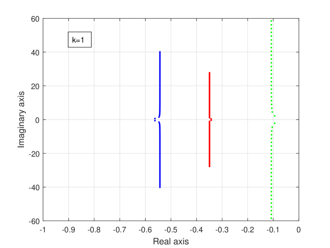
Figure 1. Eigenvalues of $\mathcal{A}$ in the complex plane for $|n|$ varies from $1$ to $30$ when $\mu=\rho_{s}=u_{s}=b=1$ and k=1.

For the case of multiple eigenvalues the following results follow by introducing generalized eigenfunctions suitably (for more details see [1, Section 7]). From the previous remark, we see that the multiple eigenvalues of $\mathcal{A}$, if at all they occur, are only finitely many. Since the asymptotic behaviors of the coefficients of the eigen vectors are needed for our later analysis, we avoid the explicit computation of the generalized eigenfunctions.

Thus, now onwards, we assume the following :

The spectrum of $$\mathcal{A} \mathcal{{Z}}_{m} {{\mathcal{H}}}$$ has simple eigenvalues on . ()

We define the family $\left\{\xi_{0}\right\}\cup\left\{\xi_{n,l}\>|\>1\leqslant l\leqslant 3,n\in\mathbb{Z}^{*}\right\}$ as follows :

We choose a normalized eigenfunctions of $\mathcal{A}$ for the eigenvalue $\lambda_{0}=0$ defined by

$$\xi_{0}=\frac{1}{\sqrt{2b\pi}}\begin{pmatrix}1\\ 0\\ 0\end{pmatrix},$$

and for the eigenvalue $\lambda_{n}^{l}$, the normalized eigenfunction defined by

$$\xi_{n,l}=\frac{1}{\theta_{n,l}}\begin{pmatrix}-1\vspace{1mm}\\ \frac{\lambda_{n}^{l}+inu_{s}}{{in\rho_{s}}}\vspace{1mm}\\ \frac{\mu\left(\lambda_{n}^{l}+inu_{s}\right)}{\rho_{s}\left(1+\kappa\lambda_{n}^{l}\right)}\end{pmatrix}e^{inx},\>l\in\left\{1,2,3\right\},\>n\in\mathbb{Z}^{*},$$ (2.42)

where

$$\theta_{n,l}=\sqrt{2{\pi}\left(b+\frac{\left|\lambda_{n}^{l}+inu_{s}\right|^{2}}{\rho_{s}n^{2}}+\frac{\kappa\mu\left|\lambda_{n}^{l}+inu_{s}\right|^{2}}{\rho_{s}^{2}\left|1+\kappa\lambda_{n}^{l}\right|^{2}}\right)}.$$ (2.43)

$\left|1+\kappa\lambda_{n}^{l}\right|\neq 0\left(l=1,2,3\right)$, as $-1/\kappa$ is not a root of the characteristic polynomial (2.1).
Similarly, we choose $\left\{\xi^{*}_{0}\right\}\cup\left\{\xi^{*}_{n,l}\>|\>1\leqslant l\leqslant 3,n\in\mathbb{Z}^{*}\right\}$ as follows :

$\xi^{*}_{0}$ is an eigenfunction of $\mathcal{A}^{*}$ with the eigenvalue $\lambda_{0}=0$ defined by

$$\xi^{*}_{0}=\frac{1}{\sqrt{2b\pi}}\begin{pmatrix}1\\ 0\\ 0\end{pmatrix},$$ (2.44)

and for the eigenvalue $\overline{\lambda_{n}^{l}}$, the eigenfunction defined by

$$\xi^{*}_{n,l}=\frac{1}{\psi_{n,l}}\begin{pmatrix}1\vspace{1mm}\\ \frac{\overline{\lambda_{n}^{l}}-inu_{s}}{{in\rho_{s}}}\vspace{1mm}\\ -\frac{\mu\left(\overline{\lambda_{n}^{l}}-inu_{s}\right)}{\rho_{s}\left(1+\kappa\overline{\lambda_{n}^{l}}\right)}\end{pmatrix}e^{inx},\>l\in\left\{1,2,3\right\},\>n\in\mathbb{Z}^{*},$$ (2.45)

where

$$\psi_{n,l}=\frac{\sqrt{{2\pi}}\left(-b+\frac{\left(\overline{\lambda_{n}^{l}+inu_{s}}\right)^{2}}{\rho_{s}n^{2}}-\frac{\mu\kappa\left(\overline{\lambda_{n}^{l}+inu_{s}}\right)^{2}}{\rho_{s}^{2}\left(1+\kappa\overline{\lambda_{n}^{l}}\right)^{2}}\right)}{\sqrt{\left(b+\frac{\left|\lambda_{n}^{l}+inu_{s}\right|^{2}}{\rho_{s}n^{2}}+\frac{\kappa\mu\left|\lambda_{n}^{l}+inu_{s}\right|^{2}}{\rho_{s}^{2}\left|1+\kappa\lambda_{n}^{l}\right|^{2}}\right)}}.$$ (2.46)

Here for all $n\in\mathbb{Z}^{*}$, $\psi_{n,l}\neq 0$ for $l=1,2,3$, because of the assumption (${{\mathcal{H}}}$).

The choice of this family of eigenfunctions of $\mathcal{A}$ and $\mathcal{A}^{*}$ ensures the following lemma.

Lemma 2.8.

Under the assumption (${{\mathcal{H}}}$), the families $\left\{\xi_{0}\right\}\cup\left\{\xi_{n,l}\>|\>1\leqslant l\leqslant 3,n\in\mathbb{Z}^{*}\right\}$ and $\left\{\xi^{*}_{0}\right\}\cup\left\{\xi^{*}_{n,l}\>|\>1\leqslant l\leqslant 3,n\in\mathbb{Z}^{*}\right\}$ satisfy the following bi-orthonormality relations :

$$\left\langle\xi_{0},\xi^{*}_{k,p}\right\rangle_{\mathcal{Z}}=0,\quad\left\langle\xi_{n,l},\xi^{*}_{k,p}\right\rangle_{\mathcal{Z}}=\delta_{k}^{n}\delta_{p}^{l},\>l,p\in\left\{1,2,3\right\},\>k,n\in\mathbb{Z}^{*},$$ (2.47)

$$\left\langle\xi_{0},\xi^{*}_{0}\right\rangle_{\mathcal{Z}}=1,\quad\left\langle\xi_{n,l},\xi^{*}_{0}\right\rangle_{\mathcal{Z}}=0,\>l\in\left\{1,2,3\right\},\>n\in\mathbb{Z}^{*},$$ (2.48)

where

$$\delta_{n}^{l}=\begin{cases}0,\>n\neq l\\ 1,\>n=l.\end{cases}$$

Moreover, the asymptotic behaviors of $\theta_{n,l}$ and $\psi_{n,l}$ are as follows :

$$\left|\theta_{n,l}\right|,\left|\psi_{n,l}\right|\rightarrow\sqrt{2{\pi}\left(b+\frac{\left(\beta_{l}+u_{s}\right)^{2}}{\rho_{s}}+\frac{\mu\left(\beta_{l}+u_{s}\right)^{2}}{\kappa\rho_{s}^{2}\beta_{l}^{2}}\right)},\text{ for }l=1,2,3\text{ as }|n|\rightarrow\infty.$$ (2.49)

Also if we write the eigenfunctions of $\mathcal{A}^{*}$ in the following way

$$\xi_{n,l}^{*}=\frac{1}{\psi_{n,l}}\begin{pmatrix}\alpha_{n,l}^{1}\\ \alpha_{n,l}^{2}\\ \alpha_{n,l}^{3}\end{pmatrix}e^{inx},\quad n\in\mathbb{Z}^{*},l=1,2,3,$$ (2.50)

then we have the following asymptotic behaviors

$$\alpha_{n,l}^{1}=1,\text{ for }l=1,2,3,\text{ for all }n\in\mathbb{Z}^{*},$$ (2.51)

$$\left|\alpha_{n,l}^{2}\right|\rightarrow\left|\frac{\beta_{l}+u_{s}}{\rho_{s}}\right|,\text{ for }l=1,2,3,\text{ as }|n|\rightarrow\infty,$$ (2.52)

$$\left|\alpha_{n,l}^{3}\right|\rightarrow\left|\frac{\mu\left(\beta_{l}+u_{s}\right)}{\kappa\rho_{s}\beta_{l}}\right|,\text{ for }l=1,2,3,\text{ as }|n|\rightarrow\infty.$$ (2.53)

Now, we show that the eigenfunctions of $\mathcal{A}$ form a Riesz basis in $\mathcal{Z}_{m}$. Recall from (2.1) that $\left\{\phi_{0,1},\phi_{n,1},\phi_{n,2},\phi_{n,3}|n\in\mathbb{Z}^{*}\right\}$ forms an orthonormal basis in $\mathcal{Z}_{m}$.

For the definition of Riesz basis in $\mathcal{Z}_{m}$, we refer [35, Definition 2.5.1, Chapter 2, Section 2.5]. In other words, the sequence $\left\{\xi_{0}\right\}\cup\left\{\xi_{n,l}\>|\>1\leqslant l\leqslant 3\right\}_{n\in\mathbb{Z}^{*}}$ forms a Riesz basis in $\mathcal{Z}_{m}$ if there exists an invertible operator $Q\in\mathcal{L}\left(\mathcal{Z}_{m}\right)$ such that

$$Q\phi_{0,1}=\xi_{0},\>Q\phi_{n,1}=\xi_{n,1},\>Q\phi_{n,2}=\xi_{n,2},\>Q\phi_{n,3}=\xi_{n,3},\>\forall n\in\mathbb{Z}^{*}.$$

Lemma 2.9.

Assume (${{\mathcal{H}}}$). Let us set $\mathcal{B}_{n}^{1}=\left\{\phi_{n,l}\>|l=1,2,3\right\}$ and $\mathcal{B}_{n}^{2}=\left\{\xi_{n,l}\>|l=1,2,3\right\}$ for all $n\in\mathbb{Z}^{*}$, where $\left\{\phi_{n,l}\right\}_{1\leqslant l\leqslant 3}$ and $\left\{\xi_{n,l}\right\}_{1\leqslant l\leqslant 3}$ are defined as in (2.1) and (2.42). Let $z_{n}\in\mathbf{V}_{n}$ be expressed in the basis $\mathcal{B}_{n}^{1}$ and $\mathcal{B}_{n}^{2}$ as follows :

$$z_{n}=\sum\limits_{p=1}^{3}c_{n,p}\phi_{n,p}=\sum\limits_{l=1}^{3}d_{n,l}\xi_{n,l},$$ (2.54)

and let the operator $\Gamma_{n}\in\mathbb{C}^{3\times 3}$ be defined by

$$\Gamma_{n}\begin{pmatrix}c_{n,1}\\ c_{n,2}\\ c_{n,3}\end{pmatrix}=\begin{pmatrix}d_{n,1}\\ d_{n,2}\\ d_{n,3}\end{pmatrix}.$$ (2.55)

Then there exist positive constants $l_{1}$ and $l_{2}$ independent of $n$ such that

$$\left\|\Gamma_{n}\right\|<l_{1},\quad\left\|\Gamma_{n}^{-1}\right\|<l_{2},\text{ for all }n\in\mathbb{Z}^{*}.$$

Proof.

Let $n\in\mathbb{Z}^{*}$ and $z_{n}$ as in (2.54). Taking inner product of $z_{n}$ with each $\xi_{n,l}^{*}$ for $1\leqslant l\leqslant 3$, and using the bi-orthonormality relation (2.47), we get

$$d_{n,l}= \left\langle z_{n},\xi_{n,l}^{*}\right\rangle_{\mathcal{{Z}}}=\sum\limits_{p=1}^{3}c_{n,p}\left\langle\phi_{n,p},\xi_{n,l}^{*}\right\rangle_{\mathcal{{Z}}}$$

$$= \sqrt{2\pi b}\frac{\overline{\alpha_{n,l}^{1}}}{\overline{\psi_{n,l}}}c_{n,1}+\sqrt{2\pi\rho_{s}}\frac{\overline{\alpha_{n,l}^{2}}}{\overline{\psi_{n,l}}}c_{n,2}+\sqrt{\frac{2\pi\kappa}{\mu}}\frac{\overline{\alpha_{n,l}^{3}}}{\overline{\psi_{n,l}}}c_{n,3}.$$

Then the matrix $\Gamma_{n}$ in (2.55) is given by

$$\Gamma_{n}=\begin{pmatrix}\sqrt{2\pi b}\frac{\overline{\alpha_{n,1}^{1}}}{\overline{\psi_{n,1}}}&\sqrt{2\pi\rho_{s}}\frac{\overline{\alpha_{n,1}^{2}}}{\overline{\psi_{n,1}}}&\sqrt{\frac{2\pi\kappa}{\mu}}\frac{\overline{\alpha_{n,1}^{3}}}{\overline{\psi_{n,1}}}\\ \sqrt{2\pi b}\frac{\overline{\alpha_{n,2}^{1}}}{\overline{\psi_{n,2}}}&\sqrt{2\pi\rho_{s}}\frac{\overline{\alpha_{n,2}^{2}}}{\overline{\psi_{n,2}}}&\sqrt{\frac{2\pi\kappa}{\mu}}\frac{\overline{\alpha_{n,2}^{3}}}{\overline{\psi_{n,2}}}\\ \sqrt{2\pi b}\frac{\overline{\alpha_{n,3}^{1}}}{\overline{\psi_{n,3}}}&\sqrt{2\pi\rho_{s}}\frac{\overline{\alpha_{n,3}^{2}}}{\overline{\psi_{n,3}}}&\sqrt{\frac{2\pi\kappa}{\mu}}\frac{\overline{\alpha_{n,3}^{3}}}{\overline{\psi_{n,3}}}\end{pmatrix}.$$ (2.56)

Then using (${{\mathcal{H}}}$), we obtain

$$\det\left(\Gamma_{n}\right)= \frac{2\pi\sqrt{2\pi b\rho_{s}\kappa\mu}}{in\rho_{s}^{2}\overline{\psi_{n,1}}\overline{\psi_{n,2}}\overline{\psi_{n,3}}}\begin{vmatrix}1&\lambda_{n}^{1}+inu_{s}&\frac{\lambda_{n}^{1}+inu_{s}}{1+\kappa\lambda_{n}^{1}}\\ 1&\lambda_{n}^{2}+inu_{s}&\frac{\lambda_{n}^{2}+inu_{s}}{1+\kappa\lambda_{n}^{2}}\\ 1&\lambda_{n}^{3}+inu_{s}&\frac{\lambda_{n}^{3}+inu_{s}}{1+\kappa\lambda_{n}^{3}}\end{vmatrix}$$

$$= \frac{2\pi\kappa\sqrt{2\pi b\rho_{s}\kappa\mu}}{in\rho_{s}^{2}\overline{\psi_{n,1}}\overline{\psi_{n,2}}\overline{\psi_{n,3}}}\frac{\left(\lambda_{n}^{1}-\lambda_{n}^{2}\right)\left(\lambda_{n}^{1}-\lambda_{n}^{3}\right)\left(\lambda_{n}^{2}-\lambda_{n}^{3}\right)\left(1-\kappa inu_{s}\right)}{\left(1+\kappa\lambda_{n}^{1}\right)\left(1+\kappa\lambda_{n}^{2}\right)\left(1+\kappa\lambda_{n}^{3}\right)}\neq 0.$$ (2.57)

Using (2.11) and (2.49), we get

$$\left|\det\left(\Gamma_{n}\right)\right|\rightarrow C\text{ as }|n|\rightarrow\infty,$$

where $C$ is a positive constant. Thus, for each $n\in\mathbb{Z}^{*},\Gamma_{n}$ is invertible with the inverse $\Gamma_{n}^{-1}$.

From the matrix $\Gamma_{n}$, using (2.49), (2.51), (2.52) and (2.53), we get a positive constant $l_{1}$ independent of $n$ such that

$$\left\|\Gamma_{n}\right\|<l_{1},\>\forall\>n\in\mathbb{Z}^{*}.$$

Similarly, we can get a positive constant $l_{2}$ independent of $n$ such that

$$\left\|\Gamma_{n}^{-1}\right\|<l_{2},\>\forall\>n\in\mathbb{Z}^{*}.$$

∎

Using 2.9 and from the second part of [35, Proposition 2.5.3, Chapter 2, Section 2.5], we can see that the eigenfunctions of $\mathcal{A}$, $\big{\{}\xi_{0},\xi_{n,l}\>|1\leqslant l\leqslant 3,\>n\in\mathbb{Z}^{*}\big{\}}$ forms a Riesz basis in $\mathcal{Z}_{m}$. Also, using [35, Proposition 2.8.6, Chapter 2, Section 2.8], [35, Definition 2.6.1, Chapter 2, Section 2.6] and 2.8, we obtain $\left\{\xi_{0}^{*},\xi^{*}_{n,l}\>|1\leqslant l\leqslant 3,\>n\in\mathbb{Z}^{*}\right\}$ forms a Riesz basis in $\mathcal{Z}_{m}$.

Proposition 2.10.

Assume (${{\mathcal{H}}}$) holds. Then any $z\in{\mathcal{{Z}}_{m}}$ can be uniquely represented as

$$z=\sum\limits_{n\in\mathbb{Z}^{*}}\sum\limits_{l=1}^{3}\left\langle z,\xi^{*}_{n,l}\right\rangle_{\mathcal{{Z}}}\xi_{n,l}+\left\langle z,\xi^{*}_{0}\right\rangle_{\mathcal{{Z}}}\xi_{0}.$$ (2.58)

There exist positive numbers $C_{1}$ and $C_{2}$ such that

$$C_{1}\left(\left|\left\langle z,\xi^{*}_{0}\right\rangle\right|^{2}+\sum_{n\in\mathbb{Z}^{*}}\sum_{l=1}^{3}\left|\left\langle z,\xi^{*}_{n,l}\right\rangle\right|^{2}\right)\leqslant\left\|z\right\|^{2}_{{\mathcal{{Z}}}}\leqslant C_{2}\left(\left|\left\langle z,\xi^{*}_{0}\right\rangle\right|^{2}+\sum_{n\in\mathbb{Z}^{*}}\sum_{l=1}^{3}\left|\left\langle z,\xi^{*}_{n,l}\right\rangle\right|^{2}\right).$$ (2.59)

Similarly, any $z\in\mathcal{{Z}}_{m}$ can be uniquely represented in the basis $\left\{\xi_{0}^{*}\right\}\cup\{\xi^{*}_{n,l}\>|1\leqslant l\leqslant 3,\>n\in\mathbb{Z}^{*}\}$ by

$$z=\sum\limits_{n\in\mathbb{Z}^{*}}\sum\limits_{l=1}^{3}\left\langle z,\xi_{n,l}\right\rangle_{\mathcal{{Z}}}\xi^{*}_{n,l}+\left\langle z,\xi_{0}\right\rangle_{\mathcal{{Z}}}\xi^{*}_{0},$$ (2.60)

and

$$\frac{1}{C_{2}}\left(\left|\left\langle z,\xi_{0}\right\rangle\right|^{2}+\sum_{n\in\mathbb{Z}^{*}}\sum_{l=1}^{3}\left|\left\langle z,\xi_{n,l}\right\rangle\right|^{2}\right)\leqslant\left\|z\right\|^{2}_{{\mathcal{{Z}}}}\leqslant\frac{1}{C_{1}}\left(\left|\left\langle z,\xi_{0}\right\rangle\right|^{2}+\sum_{n\in\mathbb{Z}^{*}}^{\infty}\sum_{l=1}^{3}\left|\left\langle z,\xi_{n,l}\right\rangle\right|^{2}\right).$$ (2.61)

As a consequence of the above proposition, from [35, Remark 2.6.4, Chapter 2, Section 2.6], we get the following result of spectrum of $\mathcal{A}$ and $\mathcal{A}^{*}$.

Theorem 2.11.

Assume (${{\mathcal{H}}}$) holds. Then the spectrum of the operator $(\mathcal{A},\mathcal{D}(\mathcal{A};\mathcal{{Z}}_{m}))$ and $(\mathcal{A}^{*},\mathcal{D}(\mathcal{A}^{*};\mathcal{{Z}}_{m}))$ are given by

$$\sigma(\mathcal{A}) =\left\{\lambda_{0}=0,\lambda_{n}^{j},\>n\in\mathbb{Z}^{*},\>j=1,2,3\right\},$$

$$\sigma(\mathcal{A}^{*}) =\left\{\lambda_{0},\overline{\lambda_{n}^{j}},\>n\in\mathbb{Z}^{*},\>j=1,2,3\right\}.$$

3. Interior controllability

This section is devoted to the exact controllability of the system (1.4) by means of localized interior control acting in any of the equations. Our proof relies on the duality between the controllability of the system and the observability of the corresponding adjoint system. Here we only prove the exact controllability result when the control acts only in the density equation. For the other two cases, the proofs follow in a similar fashion.

We recall the final state observability of $(\mathcal{A}^{*},\mathcal{B}^{*}):$ For $(\mathcal{A}^{*},\mathcal{D}(\mathcal{A}^{*};\mathcal{{Z}}_{m}))$ defined in (2.6)-(2.7) and $(\sigma_{T},v_{T},\tilde{S}_{T})^{\top}\in\mathcal{{Z}}_{m},$ we set

$$(\sigma(t),v(t),\tilde{S}(t))^{\top}=\mathbb{T}_{T-t}^{*}(\sigma_{T},v_{T},\tilde{S}_{T})^{\top}\qquad(t\in[0,T]),$$

where $\mathbb{T}^{*}$ is the $C^{0}$-semigroup generated by $(\mathcal{A}^{*},\mathcal{D}(\mathcal{A}^{*};\mathcal{{Z}}_{m}))$ on $\mathcal{{Z}}_{m}$. In view of 2.3, $(\sigma,v,\tilde{S})^{\top}$ belongs to $C([0,T];\mathcal{{Z}}_{m})$ and satisfies:

$$\begin{cases}\partial_{t}\sigma+u_{s}\partial_{x}\sigma+{\rho_{s}}\partial_{x}v=0&\mbox{ in }(0,T)\times(0,2\pi),\\ \partial_{t}v+b\partial_{x}\sigma+u_{s}\partial_{x}v-\frac{1}{\rho_{s}}\partial_{x}\tilde{S}=0&\mbox{ in }(0,T)\times(0,2\pi),\\ \partial_{t}\tilde{S}-\frac{1}{\kappa}\tilde{S}-\frac{\mu}{\kappa}\partial_{x}v=0&\mbox{ in }(0,T)\times(0,2\pi),\\ \sigma(t,0)=\sigma(t,2\pi),v(t,0)=v(t,2\pi),\>\tilde{S}(t,0)=\tilde{S}(t,2\pi),&\mbox{ in }(0,T),\\ \sigma(T,x)=\sigma_{T}(x),\quad v(T,x)=v_{T}(x),\quad\tilde{S}(T,x)=\tilde{S}_{T}(x)&\mbox{ in }(0,2\pi).\end{cases}$$ (3.1)

Here, at first we discuss a standard approach to deduce the observability inequality for the adjoint system (3.1) which essentially gives the exact controllability of the main system (1.4). Let us consider the linear map $\mathcal{F}_{T}:L^{2}(0,T,L^{2}(0,2\pi)\to(L^{2}(0,2\pi))^{3}$ by $\mathcal{F}_{T}(f_{1})=\left(\rho(T,\cdot),u(T,\cdot),S(T,\cdot)\right)^{\top}$ where $(\rho,u,S)^{\top}$ is the solution of the system (1.4) with $(\rho_{0},u_{0},S_{0})^{\top}=(0,0,0)^{\top}$ and $f_{2}=f_{3}=0$. It is clear that exact controllability of (1.4) is equivalent to the surjectivity of the linear map $\mathcal{F}_{T}$. Note that the map $\mathcal{F}_{T}$ is surjective if and only if there exists a constant $C>0$ such that the following inequality holds:

$$\left\|\mathcal{F}_{T}^{*}{z}\right\|_{L^{2}(0,T,L^{2}(0,2\pi)}\geq C\left\|z\right\|_{(L^{2}(0,2\pi))^{3}},\,\text{ for all }z\in(L^{2}(0,2\pi))^{3}.$$ (3.2)

A direct computation shows that $\mathcal{F}_{T}^{*}((\sigma_{T},v_{T},\tilde{S}_{T})^{\top})=\mathbbm{1}_{\mathcal{O}_{1}}\sigma$, where $(\sigma,v,\tilde{S})$ is the solution of the adjoint system (3.1) with the terminal data $(\sigma_{T},v_{T},\tilde{S}_{T})$. Thus the exact controllability of the system (1.4) is equivalent to the following observability inequality:

Proposition 3.1.

Let $T>0$. Assume $f_{2}=0=f_{3}$. Then the system (1.4) is exactly controllable in $\mathcal{{Z}}_{m}$ at time $T>0$ using a control $f_{1}$ in $L^{2}(0,T;L^{2}(0,2\pi))$ with support in $\mathcal{O}_{1}$ acting only in the density equation, if and only if, there exists a positive constant $C_{T}>0$ such that for any $(\sigma_{T},v_{T},\tilde{S}_{T})^{\top}\in\mathcal{{Z}}_{m}$, $(\sigma,v,\tilde{S})^{\top}$, the solution of (3.1), satisfies the following observability inequality:

$$\int_{0}^{2\pi}|\sigma_{T}(x)|^{2}\ {\rm d}x\;+\;\int_{0}^{2\pi}|v_{T}(x)|^{2}\ {\rm d}x+\;\int_{0}^{2\pi}|\tilde{S}_{T}(x)|^{2}\ {\rm d}x\leqslant C_{T}\int_{0}^{T}\int_{\mathcal{O}_{1}}|\sigma(t,x)|^{2}\,{\rm d}x\,{\rm d}t.$$ (3.3)

Next, we prove Theorem 1.2 by showing the observability inequality (3.3) using the following Ingham-type inequality.

Proposition 3.2.

Let $T>{2\pi}\left(\frac{1}{|\beta_{1}|}+\frac{1}{|\beta_{2}|}+\frac{1}{|\beta_{3}|}\right)$ and $M\in\mathbb{N}$. Then there exist positive constants $C$ and $C_{1}$ depending on $T$ such that for $g(t)=\displaystyle\sum_{|n|\geq M}\sum_{l=1}^{3}{a_{n}^{l}e^{\overline{\lambda_{n}^{l}}(T-t)}}$ with $\displaystyle{\sum_{|n|\geq M}}\sum_{l=1}^{3}|a_{n}^{l}|^{2}<\infty$, the following inequality holds:

$$C\sum_{|n|\geq M}\sum_{l=1}^{3}|a_{n}^{l}|^{2}\leqslant\int_{0}^{T}|g(t)|^{2}\,{\rm d}t\leqslant C_{1}\sum_{|n|\geq M}\sum_{l=1}^{3}|a_{n}^{l}|^{2}.$$ (3.4)

Proof.

The proof follows trivially from (7.22) of Section 7 by suitable choices of $\{a_{n}^{l}\}$ and a change of variable. ∎

3.1. Proof of Theorem 1.2:

Let $(\sigma_{T},v_{T},\tilde{S}_{T})^{\top}\in\mathcal{{Z}}_{m}.$ From 2.10, we have

$$\begin{pmatrix}\sigma_{T}\\ v_{T}\\ \tilde{S}_{T}\end{pmatrix}=\sum\limits_{n\in\mathbb{Z}^{*}}\sum\limits_{l=1}^{3}c_{n,l}\xi^{*}_{n,l}+c_{0}\xi_{0}^{*},\quad\mathrm{with}\quad\sum\limits_{n\in\mathbb{Z}^{*}}\sum\limits_{l=1}^{3}\left|c_{n,l}\right|^{2}+\left|c_{0}\right|^{2}<\infty.$$ (3.5)

Then the corresponding solution $(\sigma(t),v(t),\tilde{S}(t))^{\top}$ of the adjoint problem (3.1) can be written as

$$\begin{pmatrix}\sigma\\ v\\ \tilde{S}\end{pmatrix}(t,x)=\sum\limits_{n\in\mathbb{Z}^{*}}\sum\limits_{l=1}^{3}c_{n,l}e^{\overline{\lambda_{n}^{l}}(T-t)}\xi^{*}_{n,l}(x)+c_{0}e^{\overline{\lambda_{0}}(T-t)}\xi_{0}^{*}(x).$$ (3.6)

In particular, using the expression of $\xi^{*}_{0}$ and $\xi^{*}_{n,l}$ ( eq. (2.44), (2.45) and (2.50)), from (3.6) we get

$$\sigma(t,x)=\sum\limits_{n\in\mathbb{Z}^{*}}^{\infty}\sum\limits_{l=1}^{3}\frac{c_{n,l}}{\psi_{n,l}}e^{\overline{\lambda_{n}^{l}}(T-t)}e^{inx}+\frac{c_{0}}{\sqrt{2b\pi}},\quad\forall\,t\in(0,T),\quad x\in(0,2\pi),$$ (3.7)

$$v(t,x)=\sum\limits_{n\in\mathbb{Z}^{*}}^{\infty}\sum\limits_{l=1}^{3}\frac{c_{n,l}}{\psi_{n,l}}\alpha_{n,l}^{2}e^{\overline{\lambda_{n}^{l}}(T-t)}e^{inx},\quad\forall\,t\in(0,T),\quad x\in(0,2\pi),$$ (3.8)

$$\tilde{S}(t,x)=\sum\limits_{n\in\mathbb{Z}^{*}}^{\infty}\sum\limits_{l=1}^{3}\frac{c_{n,l}}{\psi_{n,l}}\alpha_{n,l}^{3}e^{\overline{\lambda_{n}^{l}}(T-t)}e^{inx},\quad\forall\,t\in(0,T),\quad x\in(0,2\pi).$$ (3.9)

Since $\left\{e^{inx},x\in(0,2\pi)\right\}_{n\in\mathbb{Z}}$ is an orthonormal basis in $L^{2}\left(0,2\pi\right)$ and $\{e^{inx},$ $x\in(0,2\pi)\}_{n\in\mathbb{Z}^{*}}$ is an orthonormal basis in $L_{m}^{2}\left(0,2\pi\right)$, then using Parseval’s identity, we get

$$\int_{0}^{2\pi}|\sigma^{T}(x)|^{2}\ {\rm d}x\;+\;\int_{0}^{2\pi}|v^{T}(x)|^{2}\ {\rm d}x+\;\int_{0}^{2\pi}|\tilde{S}^{T}(x)|^{2}\ {\rm d}x$$

$$= \sum\limits_{n\in\mathbb{Z}^{*}}^{\infty}\left(\left|\sum\limits_{l=1}^{3}\frac{c_{n,l}}{\psi_{n,l}}+\frac{c_{0}}{\sqrt{2b\pi}}\right|^{2}+\left|\sum\limits_{l=1}^{3}\frac{c_{n,l}}{\psi_{n,l}}\alpha_{n,l}^{2}\right|^{2}+\left|\sum\limits_{l=1}^{3}\frac{c_{n,l}}{\psi_{n,l}}\alpha_{n,l}^{3}\right|^{2}\right).$$ (3.10)

Now using (2.52) and (2.53), we get a positive constant $C$, independent of $n$ and a large $N\in\mathbb{N}$, such that

$$\sum\limits_{|n|>N}\left(\left|\sum\limits_{l=1}^{3}\frac{c_{n,l}}{\psi_{n,l}}+\frac{c_{0}}{\sqrt{2b\pi}}\right|^{2}+\left|\sum\limits_{l=1}^{3}\frac{c_{n,l}}{\psi_{n,l}}\alpha_{n,l}^{2}\right|^{2}+\left|\sum\limits_{l=1}^{3}\frac{c_{n,l}}{\psi_{n,l}}\alpha_{n,l}^{3}\right|^{2}\right)$$

$$\leqslant C\left(\sum\limits_{|n|>N}\sum\limits_{l=1}^{3}\left|\frac{c_{n,l}}{\psi_{n,l}}\right|^{2}+\left|\frac{c_{0}}{\sqrt{2b\pi}}\right|^{2}\right).$$ (3.11)

Let us define

$$a_{n}^{l}(x)=\frac{c_{n,l}}{\psi_{n,l}}e^{inx},\text{ for }|n|>N,l=1,2,3,\text{ and }x\in(0,2\pi).$$

Using (2.49) and (3.5), we have $\displaystyle{\sum_{|n|\geq N}}\sum_{l=1}^{3}|a_{n}^{l}(x)|^{2}<\infty$. Thanks to 3.2, for $T>{2\pi}\left(\frac{1}{|\beta_{1}|}+\frac{1}{|\beta_{2}|}+\frac{1}{|\beta_{3}|}\right)$, we have

$$\sum\limits_{|n|>N}\sum\limits_{l=1}^{3}\left|\frac{c_{n,l}}{\psi_{n,l}}e^{inx}\right|^{2}\leqslant C\int_{0}^{T}\left|\sum\limits_{\left|n\right|>N}\sum_{l=1}^{3}\frac{c_{n,l}}{\psi_{n,l}}e^{inx}e^{\overline{\lambda_{n}^{l}}(T-t)}\right|^{2}\,{\rm d}t.$$

Integrating both sides over $\mathcal{O}_{1}$, we get

$$\sum\limits_{|n|>N}\sum\limits_{l=1}^{3}\left|\frac{c_{n,l}}{\psi_{n,l}}\right|^{2}\leqslant C\int_{0}^{T}\int_{\mathcal{O}_{1}}\left|\sum\limits_{\left|n\right|>N}\sum_{l=1}^{3}\frac{c_{n,l}}{\psi_{n,l}}e^{inx}e^{\overline{\lambda_{n}^{l}}(T-t)}\right|^{2}\,{\rm d}x\,{\rm d}t.$$ (3.12)

Therefore only finitely many terms are leaving. Since by ${{\mathcal{H}}}$, all the eigenvalues are distinct, then the missing finitely many exponential ( for $|n|\leqslant N$) can be added one by one in the inequality (3.12) as the required gap condition for the eigenvalues holds. For similar details one can see [29, Chapter 4, Theorem 4.3 ].

Thus for $T>{2\pi}\left(\frac{1}{|\beta_{1}|}+\frac{1}{|\beta_{2}|}+\frac{1}{|\beta_{3}|}\right)$, we get

$$\sum\limits_{n\in\mathbb{Z}^{*}}\sum\limits_{l=1}^{3}\left|\frac{c_{n,l}}{\psi_{n,l}}\right|^{2}+\left|\frac{c_{0}}{\sqrt{2b\pi}}\right|^{2} \leqslant C\int_{0}^{T}\int_{\mathcal{O}_{1}}\left|\sum\limits_{n\in\mathbb{Z}^{*}}\sum_{l=1}^{3}\frac{c_{n,l}}{\psi_{n,l}}e^{inx}e^{\overline{\lambda_{n}^{l}}(T-t)}+\frac{c_{0}}{\sqrt{2b\pi}}\right|^{2}{\rm d}x\,{\rm d}t$$

$$=C\int_{0}^{T}\int_{\mathcal{O}_{1}}\left|\sigma(t,x)\right|^{2}{\rm d}x\,{\rm d}t.\>(\text{ using }\eqref{nmaxrepsigma})$$ (3.13)

Therefore using (3.1), (3.1) and (3.1), we obtain (3.3). Then by 3.1, we conclude Theorem 1.2.∎

Remark 3.3.

In the proof of Theorem 1.2, i.e, in the proof of the observability inequality (3.1), we assume that all the eigenvalues of $\mathcal{A}$ are simple to get the Ingham-type inequality for full class of exponentials $\{e^{-\overline{\lambda_{n}^{l}}t}:n\in\mathbb{Z}^{*},l\in\{1,2,3\}\}.$ In 2.7, we have mentioned that the spectrum of $\mathcal{A}$ may have finite number of multiple eigenvalues. In this case also, one can prove the observability inequality with a slight modification of the technique for simple eigenvalue case. Details analysis can be found in [10, Section 4.1]. One can also refer to the book [26, Remarks, Page 178] for a version of Ingham inequality with repeated eigenvalues.

4. Boundary controllability

In this section, we will discuss the boundary controllability of the compressible Navier–Stokes system with Maxwell’s law (1.9) with any of the boundary conditions (1.10), (1.11) and (1.12). At first, we study the boundary controllability of the system (1.9), when the control acts only in density.

4.1. Control in density

Let us consider the system (1.9) with (1.10). For the reader’s convenience, we recall the system:

$$\left.\begin{aligned} &\partial_{t}\rho+u_{s}\partial_{x}\rho+\rho_{s}\partial_{x}u=0,\qquad&&\text{in }(0,T)\times(0,2\pi),\\ &\partial_{t}u+u_{s}\partial_{x}u+a\gamma{\rho_{s}}^{\gamma-2}\partial_{x}\rho-\frac{1}{\rho_{s}}\partial_{x}S=0,\qquad&&\text{in }(0,T)\times(0,2\pi),\\ &\partial_{t}S+\frac{1}{\kappa}S-\frac{\mu}{\kappa}\partial_{x}u=0,\qquad&&\text{in }(0,T)\times(0,2\pi),\\ &\rho(t,0)=\rho(t,2\pi)+q(t),\>u(t,0)=u(t,2\pi),\>S(t,0)=S(t,2\pi),\qquad&&t\in(0,T),\\ &\rho(0,x)=\rho_{0}(x),\quad u(0,x)=u_{0}(x),\quad S(0,x)=S_{0}(x),\qquad&&x\in(0,2\pi).\end{aligned}\right\}$$ (4.1)

4.1.1. Well-posedness

Like interior controllability cases, at first let us write the system (4.1) in the following abstract form:

$$\dot{z}(t)=\mathcal{A}z(t)+\mathcal{B}_{\rho}q(t),\quad t\in(0,T),\qquad z(0)=z_{0},$$ (4.2)

where we have set $z(t)=(\rho(t,\cdot),u(t,\cdot),S(t,\cdot))^{\top},$ $z_{0}=(\rho_{0},u_{0},S_{0})^{\top}$. One can identify the operator $\mathcal{A},\mathcal{B}$ through its adjoint by taking the scalar product of (4.2) with a vector of smooth functions $(\phi,\psi,\xi)$ and comparing it with (4.1). $\mathcal{A}$ is the unbounded operator given by (2.3) with its domain

$$\mathcal{D}(\mathcal{A};\mathcal{Z}_{m,m})=\left\{\begin{pmatrix}\rho\\ u\\ S\end{pmatrix}\in\mathcal{Z}_{m,m}\>:\>\left(\rho,u,S\right)^{\top}\in H^{1}(0,2\pi)\times H^{1}(0,2\pi)\times H^{1}(0,2\pi),\>\begin{aligned} &\rho(0)=\rho(2\pi),\\ &u(0)=u(2\pi),\\ &S(0)=S(2\pi).\end{aligned}\right\}.$$

The control operator $\mathcal{B}_{\rho}\in\mathcal{L}(\mathbb{C};\mathcal{D}(\mathcal{A}^{*})^{\prime})$ defined by

$$\left<{\mathcal{B}_{\rho}q(t)},{(\phi,\psi,\xi)}\right>_{\mathcal{D}(\mathcal{A}^{*})^{\prime},\mathcal{D}(\mathcal{A}^{*})}=q(t)\left(bu_{s}\overline{\phi(2\pi)}+b\rho_{s}\overline{\psi(2\pi)}\right).$$

Clearly $\mathcal{B}_{\rho}$ is well-defined as $\mathcal{B}_{\rho}q$ is continuous on $H^{1}(0,2\pi)\times H^{1}(0,2\pi)\times H^{1}(0,2\pi)$ (by the embedding theorem $H^{1}(0,2\pi)\hookrightarrow C[0,2\pi]$). Its adjoint $\mathcal{B}_{\rho}^{*}\in\mathcal{L}(\mathcal{D}(\mathcal{A}^{*});\mathbb{C})$ is

$$\mathcal{B}_{\rho}^{*}(\phi,\psi,\xi)=\mathbbm{1}_{\{x=2\pi\}}\begin{pmatrix}bu_{s}\\ b\rho_{s}\\ 0\end{pmatrix}(\phi,\psi,\xi)=bu_{s}{\phi(2\pi)}+b\rho_{s}{\psi(2\pi)}.$$ (4.3)

One can prove that the operator $\mathcal{B}_{{\rho}}$ satisfies the following so-called admissibility condition

$$\int_{0}^{T}|\mathcal{B}_{\rho}^{*}\mathbb{T}_{T-t}^{*}\Phi|^{2}\,{\rm d}t\leqslant C\left\|\Phi\right\|_{{\mathcal{Z}}},\forall\,\Phi\in\mathcal{D}(\mathcal{A}^{*}),$$ (4.4)

where $C$ is some positive constant. The proof relies on the explicit expression of the solution of the adjoint (3.1) and the right hand side inequality of (3.4). Since $\mathcal{A}$ generates a contraction semigroup and $\mathcal{B}_{\rho}$ is an admissible operator, we can prove the following well-posedness result (see Theorem $2.37$ in page 53 of [13], for more details):

Proposition 4.1.

Let $T>0$, $(\rho_{0},u_{0},S_{0})^{\top}\in L_{m}^{2}(0,2\pi)\times L_{m}^{2}(0,2\pi)\times L_{m}^{2}(0,2\pi)$ and $q\in L^{2}(0,T)$. Then the system (4.1) has a unique solution $(\rho,u,S)^{\top}\in C\left([0,T];(L^{2}(0,2\pi)^{3})\right)$ and the solution satisfies

$$\|(\rho,u,S)\|_{C([0,T];\mathcal{{Z}})}\leqslant C\Big{(}\|(\rho_{0},u_{0},S_{0})\|_{\mathcal{{Z}}}+\|q\|_{L^{2}(0,T)}\Big{)},$$

where $C=C(T)$ is a positive constant, independent of $\rho_{0},u_{0},S_{0},q$ and $t$.

4.1.2. Exact Controllability

In this section, we prove the exact controllability of the system (4.1). As interior control case, here at first we discuss the classical approach to deduce the observability inequality for the adjoint system (3.1) which essentially gives the exact controllability of the main system (4.1). Let us consider the linear map $\mathcal{F}_{T}:L^{2}(0,T)\to(L^{2}(0,2\pi))^{3}$ by $\mathcal{F}_{T}(q)=\left(\rho(T,\cdot),u(T,\cdot),S(T,\cdot)\right)^{\top}$, where $(\rho,u,S)$ is the solution of the system (4.1) with $(\rho_{0},u_{0},S_{0})=(0,0,0)$. It is clear that exact controllability for (4.1) is equivalent to the surjectivity of the map $\mathcal{F}_{T}$. Note that the map $\mathcal{F}_{T}$ is surjective if and only if there exists a constant $C>0$ such that the following inequality holds:

$$\left\|\mathcal{F}_{T}^{*}\mathbf{z}\right\|_{L^{2}(0,T)}\geq C\left\|\mathbf{z}\right\|_{(L^{2}(0,2\pi))^{3}},\,\text{ for all }\mathbf{z}\in(L^{2}(0,2\pi))^{3}.$$ (4.5)

A direct computation shows that $\mathcal{F}_{T}^{*}((\sigma_{T},v_{T},\tilde{S}_{T}))=bu_{s}\sigma(t,2\pi)+b\rho_{s}v(t,2\pi)$, where $(\sigma,v,\tilde{S})$ is the solution of the adjoint system (3.1) with the terminal data $(\sigma_{T},v_{T},\tilde{S}_{T})$. Thus we get the following proposition.

Proposition 4.2.

The system (4.1) is exactly controllable in $\mathcal{Z}_{m,m}$ at time $T>0$ using a control $q$ in $L^{2}(0,T)$ acting only in the density, if and only if, there exists a positive constant $C_{T}>0$ such that for any $(\sigma_{T},v_{T},\tilde{S}_{T})\in\mathcal{Z}_{m,m}$, $(\sigma,v,\tilde{S})$, the solution of (3.1), satisfies the following observability inequality:

$$\int_{0}^{2\pi}|\sigma_{T}(x)|^{2}\,{\rm d}x+\int_{0}^{2\pi}|v_{T}(x)|^{2}\,{\rm d}x+\int_{0}^{2\pi}|\tilde{S}_{T}(x)|^{2}\,{\rm d}x\leqslant C_{T}\int_{0}^{T}|bu_{s}\sigma(t,2\pi)+b\rho_{s}v(t,2\pi)|^{2}\,{\rm d}t.$$ (4.6)

Before giving the proof of the above observability inequality, we mention the following lemma which ensures that the observation term is nonzero.

Lemma 4.3.

Let us recall the eigen functions $\mathcal{E}(\mathcal{A}^{*})=\left\{\xi^{*}_{n,l}\>|\>1\leqslant l\leqslant 3,n\in\mathbb{Z}^{*}\right\}$ of the unbounded operator $\mathcal{A}^{*}.$ Then we have the following result:

$$\mathcal{B}_{\rho}^{*}\xi\neq 0,\forall\,\xi\in\mathcal{E}(\mathcal{A}^{*}),$$

where $\mathcal{B}_{\rho}^{*}$ is the observation operator associated to the system (4.1), defined by (4.3).

Proof.

Observe that, $\mathcal{B}_{\rho}^{*}\xi^{*}_{n,l}=\frac{b}{{\psi}_{n}^{l}}\left({u_{s}\alpha^{1}_{n,l}+\rho_{s}\alpha^{2}_{n,l}}\right).$ From the first equation of the eigen equations $\mathcal{A}^{*}\xi^{*}_{n,l}=\overline{\lambda_{n}^{l}}\xi^{*}_{n,l}$, we obtain

$$\frac{b}{{\psi}_{n}^{l}}\left({u_{s}\alpha^{1}_{n,l}+\rho_{s}\alpha^{2}_{n,l}}\right)=\frac{b\alpha_{n,l}^{1}\overline{\lambda_{n}^{l}}}{{\psi}_{n}^{l}in}=\frac{\overline{\lambda_{n}^{l}}}{{\psi}_{n}^{l}in}\neq 0\,(\text{ using }\eqref{negrealpart},\,\eqref{nmaxequ-psi_nl}).$$ (4.7)

Thus $\mathcal{B}_{\rho}^{*}\xi^{*}_{n,l}\neq 0.$ ∎

4.1.3. Proof of Theorem 1.7

Proof.

Let $(\sigma_{T},v_{T},\tilde{S}_{T})^{\top}\in\mathcal{Z}_{m,m}.$ From 2.10, we have

$$\begin{pmatrix}\sigma_{T}\\ v_{T}\\ \tilde{S}_{T}\end{pmatrix}=\sum\limits_{n\in\mathbb{Z}^{*}}\sum\limits_{l=1}^{3}c_{n,l}\,\xi^{*}_{n,l}\quad\mathrm{with}\quad\sum\limits_{n\in\mathbb{Z}^{*}}\sum\limits_{l=1}^{3}\left|c_{n,l}\right|^{2}<\infty.$$ (4.8)

Then the corresponding solution $(\sigma(t),v(t),\tilde{S}(t))^{\top}$ of the adjoint problem (3.1) can be written as

$$\begin{pmatrix}\sigma\\ v\\ \tilde{S}\end{pmatrix}(t,x)=\sum\limits_{n\in\mathbb{Z}^{*}}\sum\limits_{l=1}^{3}c_{n,l}e^{\overline{\lambda_{n}^{l}}(T-t)}\xi^{*}_{n,l}(x)$$ (4.9)

In particular, using the expression of $\xi^{*}_{n,l}$ (4.9), we get

$$\sigma(t,x)=\sum\limits_{n\in\mathbb{Z}^{*}}^{\infty}\sum\limits_{l=1}^{3}\frac{c_{n,l}}{\psi_{n,l}}e^{\overline{\lambda_{n}^{l}}(T-t)}e^{inx},\quad\forall\,t\in(0,T),\quad x\in(0,2\pi),$$ (4.10)

$$v(t,x)=\sum\limits_{n\in\mathbb{Z}^{*}}^{\infty}\sum\limits_{l=1}^{3}\frac{c_{n,l}}{\psi_{n,l}}\alpha_{n,l}^{2}e^{\overline{\lambda_{n}^{l}}(T-t)}e^{inx},\quad\forall\,t\in(0,T),\quad x\in(0,2\pi),$$ (4.11)

$$\tilde{S}(t,x)=\sum\limits_{n\in\mathbb{Z}^{*}}^{\infty}\sum\limits_{l=1}^{3}\frac{c_{n,l}}{\psi_{n,l}}\alpha_{n,l}^{3}e^{\overline{\lambda_{n}^{l}}(T-t)}e^{inx},\quad\forall\,t\in(0,T),\quad x\in(0,2\pi).$$ (4.12)

then, in a similar technique used in the proof of Theorem 1.2, we get a positive constant $C$, independent of $n$, and a large $N\in\mathbb{N}$, such that

$$\sum\limits_{|n|>N}\left(\left|\sum\limits_{l=1}^{3}\frac{c_{n,l}}{\psi_{n,l}}\right|^{2}+\left|\sum\limits_{l=1}^{3}\frac{c_{n,l}}{\psi_{n,l}}\alpha_{n,l}^{2}\right|^{2}+\left|\sum\limits_{l=1}^{3}\frac{c_{n,l}}{\psi_{n,l}}\alpha_{n,l}^{3}\right|^{2}\right)$$

$$\leqslant C\sum\limits_{|n|>N}\sum\limits_{l=1}^{3}\left|\frac{c_{n,l}}{\psi_{n,l}}\right|^{2}.$$ (4.13)

Putting $x=2\pi$ in (4.10) and (4.11), we have

$$\sigma(t,2\pi)=\sum\limits_{n\in\mathbb{Z}^{*}}^{\infty}\sum\limits_{l=1}^{3}\frac{c_{n,l}}{\psi_{n,l}}e^{\overline{\lambda_{n}^{l}}(T-t)},\quad\forall\,t\in(0,T),$$ (4.14)

$$v(t,2\pi)=\sum\limits_{n\in\mathbb{Z}^{*}}^{\infty}\sum\limits_{l=1}^{3}\frac{c_{n,l}}{\psi_{n,l}}\alpha_{n,l}^{2}\,e^{\overline{\lambda_{n}^{l}}(T-t)},\quad\forall\,t\in(0,T),$$ (4.15)

$$S(t,2\pi)=\sum\limits_{n\in\mathbb{Z}^{*}}^{\infty}\sum\limits_{l=1}^{3}\frac{c_{n,l}}{\psi_{n,l}}\alpha_{n,l}^{3}\,e^{\overline{\lambda_{n}^{l}}(T-t)},\quad\forall\,t\in(0,T).$$ (4.16)

Now the observation term becomes

$$|bu_{s}\sigma(t,2\pi)+b\rho_{s}v(t,2\pi)|=\left|\sum\limits_{n\in\mathbb{Z}^{*}}^{\infty}\sum\limits_{l=1}^{3}\frac{c_{n,l}}{\psi_{n,l}}(bu_{s}+\alpha_{n,l}^{2}b\rho_{s})e^{\overline{\lambda_{n}^{l}}(T-t)}\right|.$$ (4.17)

Using 3.2, along with (4.1.3) and (4.17), for $T>{2\pi}\left(\frac{1}{|\beta_{1}|}+\frac{1}{|\beta_{2}|}+\frac{1}{|\beta_{3}|}\right)$, we have the following inequality:

$$\sum\limits_{|n|>N}\left(\left|\sum\limits_{l=1}^{3}\frac{c_{n,l}}{\psi_{n,l}}\right|^{2}+\left|\sum\limits_{l=1}^{3}\frac{c_{n,l}}{\psi_{n,l}}\alpha_{n,l}^{2}\right|^{2}+\left|\sum\limits_{l=1}^{3}\frac{c_{n,l}}{\psi_{n,l}}\alpha_{n,l}^{3}\right|^{2}\right)$$

$$\quad\quad\leqslant C\int_{0}^{T}\left|\sum\limits_{|n|>N}\sum\limits_{l=1}^{3}\frac{c_{n,l}}{\psi_{n,l}}(u_{s}+\alpha_{n,l}^{2}b)e^{\overline{\lambda_{n}^{l}}(T-t)}\right|^{2}\,{\rm d}t.$$ (4.18)

Then by ${{\mathcal{H}}}$ and 4.3, the missing finitely many exponential ( for $|n|\leqslant N$) can be added one by one in the inequality (4.1.3) as the required gap condition for the eigenvalues holds. Thus finally we deduce the following observability inequality

$$\int_{0}^{2\pi}|\sigma_{T}(x)|^{2}\ {\rm d}x\;+\;\int_{0}^{2\pi}|v_{T}(x)|^{2}\ {\rm d}x+\;\int_{0}^{2\pi}|\tilde{S}_{T}(x)|^{2}\ {\rm d}x$$

$$\quad\quad\quad\quad\leqslant C\int_{0}^{T}\left|u_{s}\sigma(t,2\pi)+bv(t,2\pi)\right|^{2}\,{\rm d}t.$$ (4.19)

provided $T>{2\pi}\left(\frac{1}{|\beta_{1}|}+\frac{1}{|\beta_{2}|}+\frac{1}{|\beta_{3}|}\right)$. Hence Theorem 1.7 is proved. ∎

In a similar approach as density control case, we can also prove the exact controllability result (see 1.8) of the system (1.9), when control acts only on the velocity or stress. In the following sections, we just indicate the changes according to the system (1.9)-(1.11) and (1.9)-(1.12).

4.2. Control in velocity

Here the control operator $\mathcal{B}_{u}\in\mathcal{L}(\mathbb{C};\mathcal{D}(\mathcal{A}^{*})^{\prime})$ is defined by

$$\left<{\mathcal{B}_{u}r(t)},{(\phi,\psi,\xi)}\right>_{\mathcal{D}(\mathcal{A}^{*})^{\prime},\mathcal{D}(\mathcal{A}^{*})}=r\left(b\rho_{s}\overline{\phi(2\pi)}+\rho_{s}u_{s}\overline{\psi(2\pi)}-\overline{\xi(2\pi)}\right).$$

Clearly $\mathcal{B}_{u}$ is well-defined as $\mathcal{B}_{u}r$ is continuous on $H^{1}(0,2\pi)\times H^{1}(0,2\pi)\times H^{1}(0,2\pi)$ (by the embedding theorem $H^{1}(0,2\pi)\hookrightarrow C^{0}[0,2\pi]$). Its adjoint $\mathcal{B}_{u}^{*}\in\mathcal{L}(\mathcal{D}(\mathcal{A}^{*});\mathbb{C})$ is given by

$$\mathcal{B}_{u}^{*}(\phi,\psi,\xi)=\mathbbm{1}_{\{x=2\pi\}}\begin{pmatrix}b\rho_{s}\\ \rho_{s}u_{s}\\ -1\end{pmatrix}(\phi,\psi,\xi)=b\rho_{s}{\phi(2\pi)}+\rho_{s}u_{s}{\psi(2\pi)}-{\xi(2\pi)}.$$ (4.20)

As in the density control case, here also one can prove that the control operator satisfies the admissibility condition (4.4). Thus for any $(\rho_{0},u_{0},S_{0})^{\top}\in\mathcal{Z}_{m,m}$ and $r\in L^{2}(0,T)$, the system (1.9)-(1.11) has a unique solution and the solution satisfies:

$$\|(\rho,u,S)\|_{C([0,T];(L^{2}(0,2\pi)^{3})}\leqslant C\Big{(}\|(\rho_{0},u_{0},S_{0})\|_{\mathcal{Z}}+\|r\|_{L^{2}(0,T)}\Big{)},$$

where $C=C(T)$ is a positive constant, independent of $\rho_{0},u_{0},S_{0},r$ and $t$.

Proposition 4.4.

The system (1.9)-(1.11) is exactly controllable in $\mathcal{{Z}}_{m,m}$ at time $T>0$ using a boundary control $r$ in $L^{2}(0,T)$ acting only in the velocity, if and only if, there exists a positive constant $C_{T}>0$ such that for any $(\sigma_{T},v_{T},\tilde{S}_{T})^{\top}\in\mathcal{Z}_{m,m}$, $(\sigma,v,\tilde{S})$, the solution of (3.1), satisfies the following observability inequality:

$$\int_{0}^{2\pi}|\sigma_{T}(x)|^{2}\,{\rm d}x+\int_{0}^{2\pi}|v_{T}(x)|^{2}\,{\rm d}x+\int_{0}^{2\pi}|\tilde{S}_{T}(x)|^{2}\,{\rm d}x\leqslant C_{T}\int_{0}^{T}|b\rho_{s}\sigma(t,2\pi)\\ +\rho_{s}u_{s}v(t,2\pi)-\tilde{S}(t,2\pi)|^{2}\,{\rm d}t.$$ (4.21)

Lemma 4.5.

Let us recall the eigen functions $\mathcal{E}(\mathcal{A}^{*})=\left\{\xi^{*}_{n,l}\>|\>1\leqslant l\leqslant 3,n\in\mathbb{Z}^{*}\right\}$ of the unbounded operator $\mathcal{A}^{*}.$ Then we have the following result:

$$\mathcal{B}_{u}^{*}\xi\neq 0,\forall\,\xi\in\mathcal{E}(\mathcal{A}^{*}).$$

Proof.

From (4.20) and (2.50), we have

$$\mathcal{B}_{u}^{*}\xi^{*}_{n,l}=\frac{1}{\psi_{n,l}}(b\rho_{s}+\alpha_{n,l}^{2}\rho_{s}u_{s}-\alpha_{n,l}^{3}).$$ (4.22)

The second equation of the eigen-equations $\mathcal{A}^{*}\xi^{*}_{n,l}=\overline{\lambda_{n}^{l}}\xi^{*}_{n,l}$ gives

$$b\rho_{s}+\alpha_{n,l}^{2}\rho_{s}u_{s}-\alpha_{n,l}^{3}=\frac{\rho_{s}\alpha_{n,l}^{2}\overline{\lambda_{n}^{l}}}{in}.$$ (4.23)

Thus from (4.22), (4.23) and (2.45), we have

$$\mathcal{B}_{u}^{*}\xi^{*}_{n,l}=-\frac{\rho_{s}\overline{\lambda_{n}^{l}}(\overline{\lambda_{n}^{l}}-inu_{s})}{n^{2}\psi_{n,l}\rho_{s}}\neq 0,$$

since all the eigenvalues have negative real part. ∎

4.3. Control in stress

The control operator $\mathcal{B}_{S}\in\mathcal{L}(\mathbb{C};\mathcal{D}(\mathcal{A}^{*})^{\prime})$ defined by

$$\left<{\mathcal{B}_{S}p(t)},{(\phi,\psi,\xi)}\right>_{\mathcal{D}(\mathcal{A}^{*})^{\prime},\mathcal{D}(\mathcal{A}^{*})}=-p\psi(2\pi).$$

Clearly $\mathcal{B}_{S}$ is well-defined as $\mathcal{B}_{S}p$ is continuous on $H^{1}(0,2\pi)\times H^{1}(0,2\pi)\times H^{1}(0,2\pi)$ (by the embedding theorem $H^{1}(0,2\pi)\hookrightarrow C^{0}[0,2\pi]$). Its adjoint $\mathcal{B}_{S}^{*}\in\mathcal{L}(\mathcal{D}(\mathcal{A}^{*});\mathbb{C})$ is

$$\mathcal{B}_{S}^{*}(\phi,\psi,\xi)=\mathbbm{1}_{\{x=2\pi\}}\begin{pmatrix}0\\ -1\\ 0\end{pmatrix}(\phi,\psi,\xi)=-{\psi(2\pi)},$$ (4.24)

and also $\mathcal{B}_{S}^{*}\xi\neq 0,\forall\,\xi\in\mathcal{E}(\mathcal{A}^{*}).$

5. Small time lack of controllability

In this section, we study the lack of exact controllability of the system (1.4) when the localized interior control is acting on the density equation. Similar result holds true for the remaining two cases (control in velocity or control in stress). We establish the result by violating the observability inequality on an appropriate solution of the corresponding adjoint system. Our proof is in the same spirit of [3, Section 3]. We first find a candidate function as a terminal data of the transport equation and exploit the lack of null controllability of the same in small time.

Without loss of generality, we consider the control domain $\mathcal{O}_{1}=(l_{1},l_{2}),0\leqslant l_{1}<l_{2}<2\pi.$

Theorem 5.1.

Let us take $|\beta_{1}|T<\max\{l_{1},2\pi-l_{2}\}$. Then the system (1.4) is not exactly controllable in time $T$ by means of a control $f_{1}\in L^{2}\left(0,T;L^{2}(\mathcal{O}_{1})\right)$ acting on density equation.

Proof.

Since $|\beta_{1}|T<\max\{l_{1},2\pi-l_{2}\}$, there exists a nontrivial function $\hat{\sigma}_{T}\in C_{c}^{\infty}(0,2\pi)$ such that the solution of the following equation

$$\begin{cases}\hat{\sigma}_{t}-\beta_{1}\hat{\sigma}_{x}-\omega_{1}\hat{\sigma}=0,&\mbox{ in }(0,T)\times(0,2\pi),\\ \hat{\sigma}(t,0)=\hat{\sigma}(t,2\pi),&\mbox{ in }(0,T),\\ \hat{\sigma}(T,x)=\hat{\sigma}_{T}(x),&\mbox{ in }(0,2\pi),\end{cases}$$ (5.1)

satisfies that $\text{supp}(\hat{\sigma})\cap[0,T]\times\mathcal{O}_{1}=\emptyset$ (see also [3, Section 3]). We will use the asymptotic behavior of the spectrum of the linearized operator to show the lack of controllability. At first, we construct a high-frequency version of the candidate function $\hat{\sigma}_{T}$. Let $N>0$ be a fixed integer. Next, we define the polynomial

$$P^{N}(X):=\prod_{j=-N}^{N}(X-j),$$

and the function

$$\hat{\sigma}_{T}^{N}:=P^{N}\left(-i\frac{d}{dx}\right)\hat{\sigma}_{T}.$$

Since $\hat{\sigma}_{T}^{N}$ is the image of $\hat{\sigma}_{T}$ by a differential operator, we have $\text{supp}({\hat{\sigma}_{T}^{N}})\subset\text{supp}(\hat{\sigma}_{T})$. Let us write

$$\hat{\sigma}_{T}=\sum_{n\in\mathbb{Z}}a_{n}e^{inx}\text{, where }a_{n}=\int_{0}^{2\pi}e^{inx}\hat{\sigma}_{T}(x)dx,\forall n\in\mathbb{Z}.$$

Then using the definition of $P^{N}$ and $\hat{\sigma}_{T}^{N}$, we can write $\hat{\sigma}_{T}^{N}$ in the following:

$$\hat{\sigma}_{T}^{N}(x)=\sum_{n\in\mathbb{Z}}a_{n}\prod_{j=-N}^{N}\left(-i\frac{d}{dx}-j\right)e^{inx}=\sum_{n\in\mathbb{Z}}a_{n}\prod_{j=-N}^{N}\left(n-j\right)e^{inx}=\sum_{n\in\mathbb{Z}}a_{n}P^{N}(n)e^{inx},$$

for $(t,x)\in(0,T)\times(0,2\pi)$. Note that $P^{N}(n)=0$ for all $|{n}|\leqslant N$ and therefore

$$\hat{\sigma}_{T}^{N}(x)=\sum_{{|n|}\geq N+1}a_{n}P^{N}(n)e^{inx}.$$ (5.2)

Next, we denote the function $\hat{\sigma}^{N}$ is the solution of the following equation

$$\begin{cases}\hat{\sigma}^{N}_{t}-\beta_{1}\hat{\sigma}^{N}_{x}-\omega_{1}\hat{\sigma}^{N}=0,&\mbox{ in }(0,T)\times(0,2\pi),\\ \hat{\sigma}^{N}(t,0)=\hat{\sigma}^{N}(t,2\pi),&\mbox{ in }(0,T),\\ \hat{\sigma}^{N}(T,x)=\hat{\sigma}_{T}^{N}(x),&\mbox{ in }(0,2\pi).\end{cases}$$ (5.3)

Let $(\sigma^{N},v^{N},\tilde{S}^{N})$ be the solution of the following adjoint system:

$$\begin{cases}\partial_{t}\sigma^{N}+u_{s}\partial_{x}\sigma^{N}+{\rho_{s}}\partial_{x}v^{N}=0,&\mbox{ in }(0,T)\times(0,2\pi),\\ \partial_{t}v^{N}+b\partial_{x}\sigma^{N}+u_{s}\partial_{x}v^{N}-\frac{1}{\rho_{s}}\partial_{x}\tilde{S}^{N}=0,&\mbox{ in }(0,T)\times(0,2\pi),\\ \partial_{t}\tilde{S}^{N}-\frac{1}{\kappa}\tilde{S}^{N}-\frac{\mu}{\kappa}\partial_{x}v^{N}=0,&\mbox{ in }(0,T)\times(0,2\pi),\\ \sigma^{N}(t,0)=\sigma^{N}(t,2\pi),v^{N}(t,0)=v^{N}(t,2\pi),\>\tilde{S}^{N}(t,0)=\tilde{S}^{N}(t,2\pi),&\mbox{ in }(0,T),\\ \sigma^{N}(T,x)=\hat{\sigma}^{N}_{T}(x),\quad v^{N}(T,x)=\hat{v}^{N}_{T}(x),\quad\tilde{S}^{N}(T,x)=\hat{S}^{N}_{T}(x),&\mbox{ in }(0,2\pi),\end{cases}$$ (5.4)

where $\displaystyle(\hat{\sigma}^{N}_{T},\hat{v}^{N}_{T},\hat{S}^{N}_{T})=\sum_{|n|\geq N+1}c^{1}_{n}\,\xi^{*}_{n,1},\text{ where }\frac{c^{1}_{n}}{\psi_{n,1}}=a_{n}^{N}=a_{n}P^{N}(n)$ and $\psi_{n,1},\,\xi^{*}_{n,1}$ are defined in (2.50). We write the solutions of the systems (5.3) and (5.4) respectively as

$$\hat{\sigma}^{N}(t,x) =\sum_{|{n}|\geq N+1}a^{N}_{n}\,e^{(-\beta_{1}in-\omega_{1})(T-t)}e^{inx},$$ (5.5)

$$\sigma^{N}(t,x) =\sum_{|{n}|\geq N+1}a^{N}_{n}\,e^{\overline{\lambda_{n}^{1}}(T-t)}e^{inx}.$$ (5.6)

Now, we prove that the solution component $\sigma^{N}$ of (5.4) approximates the solution $\hat{\sigma}^{N}$ of (5.3). Indeed,

$$\left\|\sigma^{N}(t,\cdot)-\hat{\sigma}^{N}(t,\cdot)\right\|_{L^{2}(0,2\pi)}^{2}$$

$$\leqslant C\sum_{|{n}|\geq N+1}|{a^{N}_{n}}|^{2}\left|e^{\overline{\lambda_{n}^{1}}(T-t)}-e^{\left({-\omega_{1}-i\beta_{1}n}\right)(T-t)}\right|^{2}$$

$$\leqslant C\sum_{|{n}|\geq N+1}\frac{1}{|{n}|^{2}}|{a^{N}_{n}}|^{2},$$

for all $t\in[0,T]$ and therefore performing integration over $[0,T]$ we have

$$\left\|\sigma^{N}-\hat{\sigma}^{N}\right\|_{L^{2}(0,T,L^{2}(0,\pi))}^{2}\leqslant\frac{C}{|{N}|^{2}}\sum_{|{n}|\geq N+1}|{a^{N}_{n}}|^{2}.$$

Using triangle inequality, we deduce

$$\left\|\sigma^{N}\right\|_{L^{2}(0,T,L^{2}(\mathcal{O}_{1}))}^{2} \leqslant\left\|\sigma^{N}-\hat{\sigma}^{N}\right\|_{L^{2}(0,T,L^{2}(\mathcal{O}_{1})}^{2}+\left\|\hat{\sigma}^{N}\right\|_{L^{2}(0,T,L^{2}(\mathcal{O}_{1}))}^{2}.$$

Since the support of $\hat{\sigma}_{N}$ does not intersect the domain $[0,T]\times\mathcal{O}_{1}$, the second term of the right hand sides vanishes. Thus we get

$$\left\|\sigma^{N}\right\|_{L^{2}(0,T,L^{2}(\mathcal{O}_{1}))}^{2}\leqslant\frac{C}{|{N}|^{2}}\sum_{|{n}|\geq N+1}|{a^{N}_{n}}|^{2}.$$ (5.7)

Next, if possible we assume that the observability for the system (5.4) holds. Therefore we have the following:

$$\int_{0}^{2\pi}|\hat{\sigma}^{N}_{T}(x)|^{2}\ {\rm d}x\;+\;\int_{0}^{2\pi}|\hat{v}^{N}_{T}(x)|^{2}\ {\rm d}x+\;\int_{0}^{2\pi}|\hat{S}^{N}_{T}(x)|^{2}\ {\rm d}x\leqslant C_{T}\int_{0}^{T}\int_{\mathcal{O}_{1}}|\sigma^{N}(t,x)|^{2}\,{\rm d}x\,{\rm d}t.$$ (5.8)

Using (5.2), (5.7) (5.8), we have

$$\int_{0}^{2\pi}|\hat{\sigma}^{N}_{T}(x)|^{2}\ {\rm d}x\leqslant\left\|\hat{\sigma}^{N}\right\|_{L^{2}(0,T,L^{2}(\mathcal{O}_{1}))}^{2}\leqslant\frac{C}{|{N}|^{2}}\sum_{|{n}|\geq N+1}|{a^{N}_{n}}|^{2}=\frac{C}{|{N}|^{2}}\int_{0}^{2\pi}|\hat{\sigma}^{N}_{T}(x)|^{2}\ {\rm d}x,$$ (5.9)

which gives a contradiction. ∎

6. Rapid exponential stabilization

Let us recall the control system (1.9). The goal of this section is to study the boundary stabilization issues for (1.9) with single boundary control force. More precisely, we construct a stationary feedback law $q(t)$, $r(t)$ or $p(t)$) of the form $\Pi\left(\rho(t,\cdot),u(t,\cdot),S(t,\cdot)\right)$ such that the solution of the closed loop system (1.9) decays exponentially to zero at any prescribed decay rate. At first we describe Urquiza’s approach [36] which is the key argument of this section.

6.1. Urquiza’s method

Let us consider an abstract control system

$$\begin{cases}\dot{y}(t)=\mathcal{A}y(t)+\mathcal{B}q(t),\quad t\in(0,T),\\ y(0)=y_{0},\end{cases}$$ (6.1)

where $y(t)\in\mathcal{H},y_{0}\in\mathcal{H},q\in L^{2}(0,T)$, $\mathcal{B}$ is an unbounded operator from $\mathbb{C}$ to $\mathcal{H}$. $\mathcal{A}:D(\mathcal{A})\subset\mathcal{H}\to\mathcal{H}$ is an unbounded operator and $\mathcal{D}(\mathcal{A})$ is dense in $\mathcal{H}.$ To employ the method of Urquiza, one needs to take the following assumptions on the operator $\mathcal{A}$ and $\mathcal{B}$

• $\mathcal{A}$ is the infinitesimal generator of a strongly continuous group $\{e^{t\mathcal{A}}\}_{t\in\mathbb{R}}$ on $\mathcal{H}$.

• $\mathcal{B}:\mathbb{C}\to\mathcal{D}(\mathcal{A}^{*})^{\prime}$ is linear and continuous.

• Regularity property. For all $T>0$ there exists $C(T)>0$ such that

  $$\int_{0}^{T}\left|\mathcal{B}^{*}e^{-t\mathcal{A}^{*}}y_{T}\right|^{2}\leqslant C\left\|y_{T}\right\|^{2}_{\mathcal{H}},\quad\forall\,y_{T}\in\mathcal{D}(\mathcal{A}^{*}).$$

• Controllability property. There are two constants $T>0$ and $c(T)>0$ such that

  $$\int_{0}^{T}\left|\mathcal{B}^{*}e^{-t\mathcal{A}^{*}}y_{T}\right|^{2}\geq c\left\|y_{T}\right\|^{2}_{\mathcal{H}},\quad\forall\,y_{T}\in\mathcal{D}(\mathcal{A}^{*}).$$

These hypotheses lead to the the following stabilization result. Its proof relies on algebraic Riccati equation associated with the linear quadratic regulator problem [18]. Let us introduce the growth bound of the semigroup $\{e^{\mathcal{A}t}\}_{t\geq 0}$ of continuous linear operator as follows:

$$g(\mathcal{A})=\inf_{t>0}\frac{1}{t}\log\left\|e^{t\mathcal{A}}\right\|_{\mathcal{L}(\mathcal{H})}.$$

Theorem 6.1.

[Urquiza [36], Theorem $2.1$] Consider operators $\mathcal{A}$ and $\mathcal{B}$ under assumptions (H1)-(H4). For any $\omega>\max\left(g(-\mathcal{A}),0\right)$, we have

• The symmetric positive operator $\Lambda_{\omega}$ defined by

  $$\left<{\Lambda_{\omega}x},{z}\right>_{\mathcal{H}}=\int_{0}^{\infty}\left<{\mathcal{B}^{*}e^{-\tau(\mathcal{A}+\omega I)^{*}}x},{\mathcal{B}^{*}e^{-\tau(\mathcal{A}+\omega I)^{*}}z}\right>_{\mathbb{C}}d\tau,\,\forall\,x,z\in\mathcal{H}$$

  is coercive and is an isomorphism on $\mathcal{H}$.

• Let $\Pi_{\omega}:=-\mathcal{B}^{*}\Lambda_{\omega}^{-1}$. The operator $\mathcal{A}+\mathcal{B}\Pi_{\omega}$ with $\mathcal{D}(\mathcal{A}+\mathcal{B}\Pi_{\omega})=\Lambda_{\omega}(\mathcal{D}(\mathcal{A}^{*}))$ is the infinitesimal generator of a strongly continuous semigroup on $\mathcal{H}$.

• The closed-loop system (6.1) with $q=\Pi_{\omega}(y)$ is exponentially stable that is,

  $$\left\|e^{t(\mathcal{A}+\mathcal{B}\Pi_{\omega})}x\right\|_{\mathcal{H}}\leqslant Ce^{\left(-2\omega+g(-\mathcal{A})\right)t}\left\|x\right\|_{\mathcal{H}},\forall x\in\mathcal{H},$$

  where $C$ is a positive constant.

We utilize Theorem 6.1 to prove the complete exponential stabilization of the linearized compressible Navier-Stokes equation with Maxwell’s law (1.9)-(1.10) with boundary feedback law.

6.2. Control in density

To apply the method mentioned above we need to show that all the assumptions (H1)-(H4) hold true for our system (4.1). Let us recall the corresponding spatial operator $(\mathcal{A},\mathcal{D}(\mathcal{A};\mathcal{Z}_{m,m})$, where $\mathcal{Z}_{m,m}=L_{m}^{2}(0,2\pi)\times L_{m}^{2}(0,2\pi)\times L_{m}^{2}(0,2\pi)$.

It can be check that the operator $(\mathcal{A},\mathcal{D}(\mathcal{A};\mathcal{Z}_{m,m})$ generates a strongly continuous group $\{\mathbb{T}_{t}\}_{t\in\mathbb{R}}$ of continuous linear operator. Hence (H1) holds. Also (H2) is true, see (4.3). We get (H3) and (H4) by Ingham inequality.

6.3. Feedback control law and proof of Theorem 1.9

In this section we employ Urquiza’s method to construct the feedback law for our system (4.1). Let us take $U^{1}_{0}=(\sigma^{1}_{0},v^{1}_{0},\tilde{S}^{1}_{0}),U^{2}_{0}=(\sigma^{1}_{0},v^{1}_{0},\tilde{S}^{1}_{0})\in\mathcal{Z}_{m,m}.$ We consider the bilinear form

$$a_{w}(U^{1}_{0},U^{2}_{0})=\int_{0}^{\infty}e^{-2\omega t}\left(bu_{s}{\sigma^{1}(t,2\pi)}+b\rho_{s}{v^{1}(t,2\pi)}\right)\overline{\left(bu_{s}{\sigma^{2}(t,2\pi)}+b\rho_{s}{v^{2}(t,2\pi)}\right)}\,{\rm d}t,$$

where $U^{1}=(\sigma^{1},v^{1},\tilde{S}^{1})$ and $U^{2}=(\sigma^{2},v^{2},\tilde{S}^{2})$ are the solutions of the following systems respectively

$$\begin{cases}\partial_{t}\sigma^{1}+u_{s}\partial_{x}\sigma^{1}+{\rho_{s}}\partial_{x}v^{1}=0&\mbox{ in }(0,T)\times(0,2\pi),\\ \partial_{t}v^{1}+b\partial_{x}\sigma^{1}+u_{s}\partial_{x}v^{1}-\frac{1}{\rho_{s}}\partial_{x}\tilde{S}^{1}=0&\mbox{ in }(0,T)\times(0,2\pi),\\ \partial_{t}\tilde{S}^{1}-\frac{1}{\kappa}\tilde{S}^{1}-\frac{\mu}{\kappa}\partial_{x}v^{1}=0&\mbox{ in }(0,T)\times(0,2\pi),\\ \sigma^{1}(t,0)=\sigma^{1}(t,2\pi),v^{1}(t,0)=v^{1}(t,2\pi),\>\tilde{S}^{1}(t,0)=\tilde{S}^{1}(t,2\pi),&\mbox{ in }(0,T),\\ \left(\sigma^{1}(T,x),v^{1}(T,x),\tilde{S}^{1}(T,x)\right)=\mathbb{T}_{-T}\left(\sigma^{1}_{0}(x),v^{1}_{0}(x),\tilde{S}^{1}_{0}(x)\right)&x\in(0,2\pi).\end{cases}$$ (6.2)

and

$$\begin{cases}\partial_{t}\sigma^{2}+u_{s}\partial_{x}\sigma^{2}+{\rho_{s}}\partial_{x}v^{2}=0&\mbox{ in }(0,T)\times(0,2\pi),\\ \partial_{t}v^{2}+b\partial_{x}\sigma^{2}+u_{s}\partial_{x}v^{2}-\frac{1}{\rho_{s}}\partial_{x}\tilde{S}^{2}=0&\mbox{ in }(0,T)\times(0,2\pi),\\ \partial_{t}\tilde{S}^{2}-\frac{1}{\kappa}\tilde{S}^{2}-\frac{\mu}{\kappa}\partial_{x}v^{2}=0&\mbox{ in }(0,T)\times(0,2\pi),\\ \sigma^{2}(t,0)=\sigma^{2}(t,2\pi),v^{2}(t,0)=v^{2}(t,2\pi),\>\tilde{S}^{2}(t,0)=\tilde{S}^{2}(t,2\pi),&\mbox{ in }(0,T),\\ \left(\sigma^{2}(T,x),v^{2}(T,x),\tilde{S}^{2}(T,x)\right)=\mathbb{T}_{-T}\left(\sigma^{2}_{0}(x),v^{2}_{0}(x),\tilde{S}^{2}_{0}(x)\right)&x\in(0,2\pi).\end{cases}$$ (6.3)

Let us define the operator $\Lambda_{\omega}:\mathcal{Z}_{m,m}\to\mathcal{Z}_{m,m}$ satisfying the following

$$\left<{\Lambda_{\omega}U^{1}_{0}},{U^{2}_{0}}\right>_{\mathcal{Z}_{m,m}}=a_{\omega}(U^{1}_{0},U^{2}_{0}),\,U^{1}_{0},U^{2}_{0}\in\mathcal{Z}_{m,m}.$$ (6.4)

Next we see that

$$a_{w}(U^{1}_{0},U^{2}_{0})= \int_{0}^{\infty}e^{-2\omega t}\left(bu_{s}{\sigma^{1}(t,2\pi)}+b\rho_{s}{v^{1}(t,2\pi)}\right)\,\,\overline{\left(bu_{s}{\sigma^{2}(t,2\pi)}+b\rho_{s}{v^{2}(t,2\pi)}\right)}\,{\rm d}t$$

$$= \int_{0}^{\infty}e^{-2\omega t}{\mathcal{B}^{*}_{\rho}}U^{1}(t)\,\,\overline{{\mathcal{B}^{*}_{\rho}}U^{2}(t)}\,{\rm d}t$$

$$= \int_{0}^{\infty}e^{-2\omega t}\left({\mathcal{B}^{*}_{\rho}}\mathbb{T}^{*}_{T-t}\mathbb{T}^{*}_{-T}U^{1}_{0}\right)\overline{\left({\mathcal{B}^{*}_{\rho}}\mathbb{T}^{*}_{T-t}\mathbb{T}^{*}_{-T}U^{2}_{0}\right)}\,{\rm d}t$$

$$= \int_{0}^{\infty}e^{-2\omega t}\left({\mathcal{B}^{*}_{\rho}}\mathbb{T}^{*}_{-t}U^{1}_{0}\right)\overline{\left({\mathcal{B}^{*}_{\rho}}\mathbb{T}^{*}_{-t}U^{2}_{0}\right)}\,{\rm d}t.$$

Therefore from (6.4), we have

$$\left<{\Lambda_{\omega}U^{1}_{0}},{U^{2}_{0}}\right>_{\mathcal{Z}_{m,m}}=\int_{0}^{\infty}e^{-2\omega t}\left<{{\mathcal{B}^{*}_{\rho}}\mathbb{T}^{*}_{-t}U^{1}_{0}},{\,{\mathcal{B}^{*}_{\rho}}\mathbb{T}^{*}_{-t}U^{2}_{0}}\right>_{\mathbb{C}}\,{\rm d}t.$$ (6.5)

Thanks to Theorem 6.1, the operator $\Lambda_{\omega}$ defined by (6.4) is coercive and isomorphism. Finally, let us define the operator ${\Pi}_{\omega}:\mathcal{Z}_{m,m}\to\mathbb{C}$ by

$${\Pi}_{\omega}(\mathbf{z})=-\left(bu_{s}{\sigma^{1}_{0}(2\pi)}+b\rho_{s}{v^{1}_{0}(2\pi)}\right),$$

where $U^{1}_{0}=(\sigma^{1}_{0},v^{1}_{0},\tilde{S}^{1}_{0})$ is the solution of the following Lax-Milgram problem

$$a_{\omega}(U^{1}_{0},U^{2}_{0})=\left<{\mathbf{z}},{U^{2}_{0}}\right>,\,\forall\,U^{2}_{0}\in\mathcal{Z}_{m,m}.$$

Hence we obtain $\left<{\Lambda_{\omega}U^{1}_{0}},{U^{2}_{0}}\right>_{\mathcal{Z}_{m,m}}=\left<{\mathbf{z}},{U^{2}_{0}}\right>,\forall\,U^{2}_{0}\in\mathcal{Z}_{m,m}.$ This gives $\Lambda_{\omega}U^{1}_{0}=\mathbf{z}.$ It follows that $U^{1}_{0}=\Lambda_{\omega}^{-1}\mathbf{z}.$ Thus we have ${\Pi}_{\omega}=-{\mathcal{B}}^{*}\Lambda_{\omega}^{-1}.$ Thanks to Theorem 6.1, rapid exponential stabilization for the system (4.1) is established by means of the feedback law $q(t)={\Pi}_{\omega}(\rho(t,\cdot),v(t,\cdot),S(t,\cdot))$. More precisely, we get a positive constant $C$ such that the solution of (4.1) satisfies the following estimate

$$\left\|\rho(t,\cdot)\right\|_{L^{2}(0,2\pi)}+\left\|u(t,\cdot)\right\|_{L^{2}(0,2\pi)}+\left\|S(t,\cdot)\right\|_{L^{2}(0,2\pi)} \leqslant Ce^{-\nu t}\bigg{[}\left\|\rho_{0}\right\|_{L^{2}(0,2\pi)}+\left\|u_{0}\right\|_{L^{2}(0,2\pi)}+\left\|S_{0}\right\|_{L^{2}(0,2\pi)}\bigg{]}.$$ (6.6)

A similar process will give the complete stabilization for the control systems (1.9)-(1.11) and (1.9)-(1.12).

7. Construction of the biorthogonal family and Ingham-type inequality

This section is devoted to the proof of a suitable Ingham-type inequality which essentially helps to derive the required observability inequality. The proof of the Ingham-type inequality relies on the construction of a biorthogonal family of $\{e^{-{\lambda_{k}^{l}}t}\}_{k\in\mathbb{Z}^{*},l\in\{1,2,3\}}$. All the constants used in this section while finding the relevant estimates are generic, which may vary from line to line.

Let us assume (${{\mathcal{H}}}$). We recall the expressions of the eigenvalues of $\mathcal{A}$ in the following manner.

$$\left.\begin{aligned} \lambda_{n}^{1}=&-\omega_{1}+i\beta_{1}n+O\left(\frac{1}{|n|}\right),&n\in\mathbbm{Z}^{*},\\ \lambda_{n}^{2}=&-\omega_{2}+i\beta_{2}n+O\left(\frac{1}{|n|}\right),&n\in\mathbbm{Z}^{*},\\ \lambda_{n}^{3}=&-\omega_{3}+i\beta_{3}n+O\left(\frac{1}{|n|}\right)&n\in\mathbbm{Z}^{*}.\end{aligned}\right\}$$ (7.1)

We further denote the following notation:

$$\Sigma=\{(n,j):n\in\mathbb{Z}^{*},1\leqslant j\leqslant 3\}.$$

Lemma 7.1 (Gap properties of the spectrum).

For any $(n,j),(k,l)\in\Sigma$, there exists $\hat{C}>0$ depending on $\omega_{1},\omega_{2},\omega_{3},\beta_{1},\beta_{2},\beta_{3}$, such that

$$\left|\lambda_{n}^{j}-\lambda_{k}^{l}\right|\geq\hat{C}.$$ (7.2)

Proof.

Note that $\omega_{1},\omega_{2},\omega_{3}$ are distinct and $\beta_{1},\beta_{2},\beta_{3}$ are also distinct. Thanks to the asymptotic behavior of the eigenvalues (7.1), we have a large $N\in\mathbb{N}$ such that for $(n,j),(k,j)\in\Sigma,\text{ with }n\neq k$ and $|n|,|k|>N$,

$$\left|\lambda_{n}^{j}-\lambda_{k}^{j}\right|\geq\left|\Im({\lambda_{n}^{j}-\lambda_{k}^{j}})\right|\geq C\left|\beta_{j}(n-k)\right|\geq C|\beta_{j}|.$$

Analogously, for $(n,j),(k,l)\in\Sigma,j\neq l$, $|n|,|k|>N$, we have

$$\left|\lambda_{n}^{j}-\lambda_{k}^{l}\right|\geq\left|\Re({\lambda_{n}^{j}-\lambda_{k}^{l}})\right|\geq C\left|\omega_{j}-\omega_{l}\right|.$$

As the eigenvalues are simple, we also find the gap condition (7.2) for finite number of the lower frequencies. ∎

Let us first define the exponential type and sine type functions.

Definition 7.2 (Entire functions of exponential type).

An entire function $f$ is said to be of exponential type $A$ if there exist positive constants $A,B$ such that

$$|f(z)|\leqslant Be^{A|z|},\,z\in\mathbb{C},$$

and of exponential type at most $A$, if for any $\epsilon>0$, there exits $B_{\epsilon}>0$ such that

$$|f(z)|\leqslant B_{\epsilon}\,e^{(A+\epsilon)|z|},\,z\in\mathbb{C}.$$

Definition 7.3.

(Sine type function) An entire function $f$ of exponential type $\pi$ is said to be of sine type if

• the zeros of $f(z)$, say $\mu_{k}$ satisfy the gap condition, i.e., there exists $\delta>0$ such that $|\mu_{k}-\mu_{l}|>\delta$ for $k\neq l$, and

• there exist positive constants $C_{1}$,$C_{2}$ and $C_{3}$ such that

  $$C_{1}e^{\pi|y|}\leqslant|f(x+iy)|\leqslant C_{2}e^{\pi|y|},\,\forall\,x,y\in\mathbb{R}\text{ with }|y|\geq C_{3}.$$

The following proposition states some important properties of sine-type functions:

Proposition 7.4.

Let $f$ be a sine type function, and let $\{\mu_{k}\}_{k\in\mathcal{I}}$ with $\mathcal{I}\subset\mathbb{Z}$ be its sequence of zeros. Then, we have:

• for any $\epsilon>0$, there exist constants $K_{\epsilon},\tilde{K}_{\epsilon}>0$ such that

  $$K_{\epsilon}e^{\pi|y|}\leqslant|f(x+iy)|\leqslant\tilde{K}_{\epsilon}e^{\pi|y|},\text{ if dist$\left(x+iy,\{\mu_{k}\}\right)>\epsilon$},$$

• there exist some constants $K_{1},K_{2}>0$ such that

  $$K_{1}<|f^{\prime}(\mu_{k})|<K_{2},\quad\forall k\in\mathcal{I}.$$

The main goal of this section is to find a class of entire functions $\mathcal{G}=\{\Psi_{k}^{j}\}_{(k,j)\in\Sigma}$ with the following properties:

• The family $\mathcal{G}$ contains entire functions of exponential type $\frac{T}{2}$. That means there exists a positive constant $C$ such that

  $$\left|\Psi_{k}^{j}(z)\right|\leqslant Ce^{\frac{T}{2}\left|z\right|},\quad\forall z\in\mathbb{C},\,\,(k,j)\in\Sigma.$$ (7.3)

• All the members of $\mathcal{G}$ are square-integrable on the real line, i.e.,

  $$\int_{\mathbb{R}}\left|\Psi_{k}^{j}(x)\right|^{2}\,{\rm d}x<\infty.$$ (7.4)

Let us now state the celebrated Paley-Wiener theorem, from which we can conclude about the desired biorthogonal family using the family $\mathcal{G}$.

Theorem 7.5 (Paley-Wiener).

Let $f$ be an entire function of exponential type $A$ and suppose

$$\int_{-\infty}^{\infty}|f(x)|^{2}\,{\rm d}x<\infty.$$

Then there exists a function $\phi\in L^{2}(-A,A)$ with the following representation

$$f(z)=\int_{-A}^{A}e^{izt}\phi(t)\,{\rm d}t,\,z\in\mathbb{C}.$$

Thus if we have the existence of such family $\mathcal{G}$ of entire functions satisfying (7.3)-(7.4), then applying the Paley-Wiener theorem for the same, one can get a family of functions $\mathcal{J}=\{\Theta_{k}^{j},\}_{(k,j)\in\Sigma}$ supported in $[-\frac{T}{2},\frac{T}{2}]$, such that the following representation holds

$$\Psi_{k}^{j}(z)=\int_{-\frac{T}{2}}^{\frac{T}{2}}e^{izt}\Theta_{k}^{j}(t)dt,\,z\in\mathbb{C}.$$ (7.5)

Clearly, $\Theta_{k}^{j}$ are the Fourier transformations of $\Psi_{k}^{j}$ respectively, for $(k,j)\in\Sigma.$ Also, by Plancharel’s Theorem, we have

$$\int_{\mathbb{R}}\left|\Psi_{k}^{j}(x)\right|^{2}=2\pi\int_{-\frac{T}{2}}^{\frac{T}{2}}\left|\Theta_{k}^{j}(t)\right|^{2}\,{\rm d}t.$$

Now we are in the position of formulating the construction of the family $\mathcal{G}$ satisfying (7.3)-(7.4). Let us first introduce the following entire function, which has simple zeros exactly at $i\overline{\lambda_{k}^{j}}:$

$$P(z)=z^{3}\prod_{(k,j)\in\Sigma}\left(1-\frac{z}{i\overline{\lambda_{k}^{j}}}\right).$$ (7.6)

Proposition 7.6.

Let $P$ be the canonical product defined in (7.6). Then $P$ is an entire function of exponential type $\pi\left(\frac{1}{|\beta_{1}|}+\frac{1}{|\beta_{2}|}+\frac{1}{|\beta_{3}|}\right)$, which satisfies the following properties:

• There exists a positive constant $C>0$ such that

  $$|P(x)|\leqslant C,\quad\forall x\in\mathbb{R}.$$ (7.7)

• There exists constant $C_{2}>0$ such that

  $$\left|P^{\prime}\left(i\overline{\lambda_{k}^{j}}\right)\right|\geq C_{2},\forall(k,j)\in\Sigma.$$ (7.8)

Proof.

Let us denote $\nu_{n}^{j}=\frac{1}{\beta_{j}}\lambda_{n}^{j}.$ thus, we have:

$$\begin{cases}\nu_{n}^{1}=-\frac{\omega_{1}}{\beta_{1}}+in+O\left(\frac{1}{|n|}\right),\\ \nu_{n}^{2}=-\frac{\omega_{2}}{\beta_{2}}+in+O\left(\frac{1}{|n|}\right),\\ \nu_{n}^{3}=-\frac{\omega_{3}}{\beta_{3}}+in+O\left(\frac{1}{|n|}\right).\end{cases}$$ (7.9)

Let us denote the products $P_{j},j\in\{1,2,3\}$ by

$$P_{j}(z)=z\prod_{k\in\mathbb{Z}^{*}}\left(1-\frac{z}{i\overline{\nu_{k}^{j}}}\right).$$ (7.10)

Thus the canonical product $P$ can be written in the following form

$$P(z)=\prod_{j\in\{1,2,3\}}\beta_{j}P_{j}\left(\frac{z}{\beta_{j}}\right).$$ (7.11)

Lemma 7.7 (Young[42], Rosier [28]).

Let $\Lambda_{k}=k+d_{k}$, where $d_{k}=d+O(k^{-1}),$ as $\left|k\right|\to\infty$ for some constant $d\in\mathbb{C}$, and that $\Lambda_{k}\neq\Lambda_{l}$ for $k\neq l.$ Then $f(z)=z\prod_{k\in\mathbb{Z}^{*}}\left(1-\frac{z}{\Lambda_{k}}\right)$ is an entire function of sine type.

Note that, $i\overline{\nu_{k}^{j}}=-i\frac{\omega_{j}}{\beta_{j}}+n+O\left(\frac{1}{|n|}\right),j\in\{1,2,3\}$. Also $i\overline{\nu_{k}^{j}}\neq i\overline{\nu_{l}^{j}},$ for $l\neq k$. Thanks to 7.7, each $P_{j}$ is a sine type function. Moreover, each of these functions is an entire function of exponential type $\pi$. Hence, $P$ is an entire function of the exponential type $\pi\left(\frac{1}{|\beta_{1}|}+\frac{1}{|\beta_{2}|}+\frac{1}{|\beta_{3}|}\right)$.

Thanks to the definition of sine-type function, for any $\epsilon>0$ there exist positive constants $C_{1},C_{2},C_{3},C_{4},$ $C_{5}$, where $C_{2}$ and $C_{3}$ depend on $\epsilon$, such that

$$\left|P_{j}(z)\right|\leqslant C_{1}^{j}e^{\pi\left|z\right|}, \>\>z\in\mathbb{C},\quad j\in\{1,2,3\},$$ (7.12)

$$C_{2}^{j}e^{\pi\left|y\right|}\leqslant\left|P_{j}(x+iy)\right|\leqslant C_{3}^{j}e^{\pi\left|y\right|},\>\> \text{if }dist\left(x+iy,\{i\overline{\nu_{j}^{k}}\}\right)>\epsilon,$$ (7.13)

$$C_{4}^{j}<\left|P_{j}^{\prime}\left(i\overline{\nu_{k}^{j}}\right)\right|<C_{5}^{j}, \>\>\forall(k,j)\in\Sigma.$$ (7.14)

Now using the above inequality (7.13) and continuity of $P_{j}$, we get a positive constant $C^{j}$ such that

$$\left|P_{j}(x)\right|\leqslant C^{j},\quad\forall\,x\in\mathbb{R}.$$ (7.15)

Therefore the estimate (7.7) holds.

Using (7.11) and (7.14) we have:

$$\left|P^{\prime}\left(i\overline{\lambda_{n}^{j}}\right)\right|=\left|P_{j}^{\prime}\left(i\overline{\nu_{n}^{j}}\right)\prod_{\begin{subarray}{c}l\in\{1,2,3\}\\ l\neq j\end{subarray}}\beta_{l}P_{l}\left(\frac{i\overline{\lambda_{n}^{j}}}{\beta_{l}}\right)\right|\geq\min_{1\leqslant j\leqslant 3}\{C_{4}^{j}\}\prod_{\begin{subarray}{c}l\in\{1,2,3\}\\ l\neq j\end{subarray}}\left|\beta_{l}P_{l}\left(\frac{i\overline{\lambda_{n}^{j}}}{\beta_{l}}\right)\right|.$$ (7.16)

Therefore to prove the estimate (7.8), we need to compute the estimate of the quantities $P_{l}\left(\frac{i\overline{\lambda_{n}^{j}}}{\beta_{l}}\right),l\neq j.$ Thanks to 7.1, we have

$$\left|\frac{i\overline{\lambda_{n}^{j}}}{\beta_{l}}-i\overline{\nu_{k}^{l}}\right|=\frac{1}{|\beta_{l}|}\left|{\overline{\lambda_{n}^{j}}}-\beta_{l}\overline{\nu_{k}^{l}}\right|=\frac{1}{|\beta_{l}|}\left|{\overline{\lambda_{n}^{j}}}-\overline{\lambda_{k}^{l}}\right|>\hat{C}.$$

Therefore using the estimate (7.13), we finally have the estimate

$$\left|P_{l}\left(\frac{i\overline{\lambda_{n}^{j}}}{\beta_{l}}\right)\right|\geq C_{2}^{l}e^{\pi\left|\frac{\omega_{j}}{\beta_{l}}\right|}.$$ (7.17)

Hence (7.16) along with (7.17) provide the estimate (7.8). ∎

Theorem 7.8.

Let $T>2\pi\left(\frac{1}{|\beta_{1}|}+\frac{1}{|\beta_{2}|}+\frac{1}{|\beta_{3}|}\right).$ Then there exists a family $\{\Theta_{n}^{j}\}_{(n,j)\in\Sigma}$ which is biorthogonal to the family of exponentials $\{e^{-{\lambda_{k}^{l}}t}\}_{(k,l)\in\Sigma}$ in $L^{2}\left(-\frac{T}{2},\frac{T}{2}\right)$, i.e.,

$$\int_{-\frac{T}{2}}^{\frac{T}{2}}\Theta_{n}^{j}(t)e^{-\overline{\lambda_{k}^{l}}t}\,{\rm d}t=\delta_{nk}\delta_{jl}.$$ (7.18)

Moreover, there exists a positive constant $C>0$ such that the following estimate holds:

$$\left\|\sum_{(n,j)\in\Sigma}a_{n}^{j}\Theta_{n}^{j}\right\|_{L^{2}\left(-\frac{T}{2},\frac{T}{2}\right)}^{2}\leqslant C\sum_{(n,j)\in\Sigma}|a_{n}^{j}|^{2},$$ (7.19)

for any finite sequence of complex numbers $\{a_{n}^{j}\}_{(n,j)\in\Sigma}$.

Proof.

Let us first define the entire function

$$\Psi_{n}^{j}(z):=\frac{P(z)}{(z-i\overline{\lambda_{n}^{j}})P^{\prime}\left(i\overline{\lambda_{n}^{j}}\right)}.$$

Clearly, $\Psi_{n}^{j}$ is a collection of entire functions of exponential type at most $\pi\left(\frac{1}{|\beta_{1}|}+\frac{1}{|\beta_{2}|}+\frac{1}{|\beta_{3}|}\right).$ Moreover, it is easy to check that

$$\int_{\mathbb{R}}\left|\Psi_{n}^{j}(x)\right|^{2}\,{\rm d}x<C.$$ (7.20)

Therefore by Paley-Wiener Theorem (Theorem 7.5), there exists a collection of functions $\{\Theta_{n}^{j}\}_{(n,j)\in\Sigma}$ supported in $[-\frac{T^{\prime}}{2},\frac{T^{\prime}}{2}]$, with $T^{\prime}=2\pi\left(\frac{1}{|\beta_{1}|}+\frac{1}{|\beta_{2}|}+\frac{1}{|\beta_{3}|}\right)$ such that the following relation holds

$$\Psi_{n}^{j}(z)=\int_{-\frac{T^{\prime}}{2}}^{\frac{T^{\prime}}{2}}e^{izt}\Theta_{n}^{j}(t)\,{\rm d}t,\,z\in\mathbb{C}.$$ (7.21)

Also, we can deduce

$$\Psi_{n}^{j}(i\overline{\lambda_{k}^{l}})=\delta_{nk}\delta_{jl},\,\,(n,j),(k,l)\in\Sigma.$$

Thus we have the family $\{\Theta_{n}^{j}\}_{(n,j)\in\Sigma}$ which is biorthogonal to the family of exponentials $\{e^{-{\lambda_{k}^{l}}t}\}_{(k,l)\in\Sigma}$ in $L^{2}\left(-\frac{T^{\prime}}{2},\frac{T^{\prime}}{2}\right)$ and by Plancharel’s Theorem and (7.20), we have

$$2\pi\int_{-\frac{T^{\prime}}{2}}^{\frac{T^{\prime}}{2}}\left|\Theta_{k}^{j}(t)\right|^{2}\,{\rm d}t=\int_{\mathbb{R}}\left|\Psi_{k}^{j}(x)\right|^{2}\,{\rm d}x\leqslant C.$$

Then using [35, Proposition 8.3.9], we have for any $T>T^{\prime}$, there exists a biorthogonal family $\{\Theta_{n}^{j}\}_{(n,j)\in\Sigma}$ of $\{e^{-{\lambda_{k}^{l}}t}\}_{(k,l)\in\Sigma}$ in $L^{2}\left(-\frac{T}{2},\frac{T}{2}\right)$ such that the estimate (7.19) holds. ∎

The following corollary is an immediate consequence of the above theorem which will essentially give us the required Ingham-type inequality.

Corollary 7.9.

Let us assume $T>2\pi\left(\frac{1}{|\beta_{1}|}+\frac{1}{|\beta_{2}|}+\frac{1}{|\beta_{3}|}\right).$ Then for any finite sequence of scalars $\{a_{n}^{j}\}_{(n,j)\in\Sigma}$, there exist two positive constants $C_{1},C_{2}$ such that the following inequality holds:

$$C_{1}\sum_{(n,j)\in\Sigma}|a_{n}^{j}|^{2}\leqslant\left\|\sum_{(n,j)\in\Sigma}a_{n}^{j}e^{-\overline{\lambda_{n}^{j}}t}\right\|_{L^{2}\left(-\frac{T}{2},\frac{T}{2}\right)}^{2}\leqslant C_{2}\sum_{(n,j)\in\Sigma}|a_{n}^{j}|^{2}.$$ (7.22)

Proof.

Using (7.18), we can deduce

$$\sum_{(n,j)\in\Sigma}|a_{n}^{j}|^{2}= \int_{-\frac{T}{2}}^{\frac{T}{2}}{\left(\sum_{(n,j)\in\Sigma}a_{n}^{j}e^{-\overline{\lambda_{n}^{j}}t}\right)}\left(\sum_{(k,l)\in\Sigma}\overline{a_{k}^{l}}\Theta_{k}^{l}(t)\right)\,{\rm d}t$$

$$\leqslant \left\|\sum_{(n,j)\in\Sigma}a_{n}^{j}e^{-\overline{\lambda_{n}^{j}}t}\right\|_{L^{2}\left(-\frac{T}{2},\frac{T}{2}\right)}\left\|\sum_{(n,j)\in\Sigma}\overline{a_{k}^{l}}\Theta_{k}^{l}\right\|_{L^{2}\left(-\frac{T}{2},\frac{T}{2}\right)}.$$ (7.23)

The inequality (7) along with (7.19) establish the left inequality of (7.22).

Straightforward estimate provides the right hand inequality. Indeed,

$$\left\|\sum_{(n,j)\in\Sigma}a_{n}^{j}e^{-\overline{\lambda_{n}^{j}}t}\right\|_{L^{2}\left(-\frac{T}{2},\frac{T}{2}\right)}^{2}\leqslant C_{2}\sum_{j=1}^{3}\left\|\sum_{n\in\mathbb{Z}^{*}}a_{n}^{j}e^{-\overline{\lambda_{n}^{j}}t}\right\|_{L^{2}\left(-\frac{T}{2},\frac{T}{2}\right)}^{2}.$$

Next, utilizing the Ingham-type inequality [1, Proposition 8.1], one can get the right hand inequality.∎

Data availability statement

This article describes entirely theoretical research. Thus, data sharing is not applicable to this article as no datasets were generated or analysed during the current study.

References

• [1] S. Ahamed and D. Mitra, Some controllability results for linearized compressible Navier-Stokes system with Maxwell’s law, Submitted, (2022) .
• [2] V. Barbu, I. Lasiecka, and R. Triggiani, Tangential boundary stabilization of Navier-Stokes equations, Mem. Amer. Math. Soc., 181 (2006), pp. x+128.
• [3] K. Beauchard, A. Koenig, and K. Le Balc’h, Null-controllability of linear parabolic transport systems, J. Éc. polytech. Math., 7 (2020), pp. 743–802.
• [4] K. Bhandari, S. Chowdhury, R. Dutta, and J. Kumbhakar, Boundary null-controllability of 1d linearized compressible navier-stokes system by one control force, 2022.
• [5] U. Biccari and S. Micu, Null-controllability properties of the wave equation with a second order memory term, Journal of Differential Equations, 267 (2019), pp. 1376–1422.
• [6] R. d. A. Capistrano-Filho, E. Cerpa, and F. A. Gallego, Rapid exponential stabilization of a boussinesq system of kdv-kdv type, Communications in Contemporary Mathematics, (2021).
• [7] E. Cerpa and E. Crépeau, Rapid exponential stabilization for a linear Korteweg-de Vries equation, Discrete Contin. Dyn. Syst. Ser. B, 11 (2009), pp. 655–668.
• [8] S. Chowdhury, R. Dutta, and S. Majumdar, Boundary controllability and stabilizability of a coupled first-order hyperbolic-elliptic system, Evol. Equ. Control Theory, 12 (2023), pp. 907–943.
• [9] S. Chowdhury and D. Mitra, Null controllability of the linearized compressible Navier-Stokes equations using moment method, J. Evol. Equ., 15 (2015), pp. 331–360.
• [10] S. Chowdhury, D. Mitra, M. Ramaswamy, and M. Renardy, Null controllability of the linearized compressible Navier Stokes system in one dimension, J. Differential Equations, 257 (2014), pp. 3813–3849.
• [11] S. S. Collis, K. Ghayour, M. Heinkenschloss, M. Ulbrich, and S. Ulbrich, Numerical solution of optimal control problems governed by the compressible Navier-Stokes equations, in Optimal control of complex structures (Oberwolfach, 2000), vol. 139 of Internat. Ser. Numer. Math., Birkhäuser, Basel, 2002, pp. 43–55.
• [12]  , Optimal control of unsteady compressible viscous flows, Internat. J. Numer. Methods Fluids, 40 (2002), pp. 1401–1429.
• [13] J.-M. Coron, Control and nonlinearity, vol. 136 of Mathematical Surveys and Monographs, American Mathematical Society, Providence, RI, 2007.
• [14] R. Datko, A linear control problem in an abstract Hilbert space, J. Differential Equations, 9 (1971), pp. 346–359.
• [15] S. Ervedoza, O. Glass, and S. Guerrero, Local exact controllability for the two- and three-dimensional compressible Navier-Stokes equations, Comm. Partial Differential Equations, 41 (2016), pp. 1660–1691.
• [16] S. Ervedoza, O. Glass, S. Guerrero, and J.-P. Puel, Local exact controllability for the one-dimensional compressible Navier-Stokes equation, Arch. Ration. Mech. Anal., 206 (2012), pp. 189–238.
• [17] S. Ervedoza and M. Savel, Local boundary controllability to trajectories for the 1D compressible Navier Stokes equations, ESAIM Control Optim. Calc. Var., 24 (2018), pp. 211–235.
• [18] F. Flandoli, I. Lasiecka, and R. Triggiani, Algebraic Riccati equations with nonsmoothing observation arising in hyperbolic and Euler-Bernoulli boundary control problems, Ann. Mat. Pura Appl. (4), 153 (1988), pp. 307–382 (1989).
• [19] A. V. Fursikov, Stabilization for the 3D Navier-Stokes system by feedback boundary control, vol. 10, 2004, pp. 289–314. Partial differential equations and applications.
• [20] G. Harris and C. Martin, The roots of a polynomial vary continuously as a function of the coefficients, Proc. Amer. Math. Soc., 100 (1987), pp. 390–392.
• [21] Y. Hu and R. Racke, Compressible navier-stokes equations with revised maxwell’s law, J. Math. Fluid Mech., 19 (2017), p. 77–90.
• [22] Y. Hu and N. Wang, Global existence versus blow-up results for one dimensional compressible navier–stokes equations with maxwell’s law, Mathematische Nachrichten, 292 (2019), pp. 826–840.
• [23] A. E. Ingham, Some trigonometrical inequalities with applications to the theory of series, Math. Z., 41 (1936), pp. 367–379.
• [24] A. Koenig and P. Lissy, Null-controllability of underactuated linear parabolic-transport systems with constant coefficients, 2023.
• [25] V. Komornik, Exact controllability and stabilization, RAM: Research in Applied Mathematics, Masson, Paris; John Wiley & Sons, Ltd., Chichester, 1994. The multiplier method.
• [26] V. Komornik and P. Loreti, Fourier series in control theory, Springer Monographs in Mathematics, Springer-Verlag, New York, 2005.
• [27] J. Kumbhakar, Null controllability of one-dimensional linearized compressible navier-stokes system in periodic setup using one boundary control, 2023.
• [28] P. Martin, L. Rosier, and P. Rouchon, Null controllability of the structurally damped wave equation with moving control, SIAM J. Control Optim., 51 (2013), pp. 660–684.
• [29] S. Micu and E. Zuazua, An introduction to the controllability of partial differential equations, Quelques questions de théorie du contrôle. Sari, T., ed., Collection Travaux en Cours Hermann, to appear, (2004).
• [30] D. Mitra, M. Ramaswamy, and M. Renardy, Interior local null controllability of one-dimensional compressible flow near a constant steady state, Math. Methods Appl. Sci., 40 (2017), pp. 3445–3478.
• [31] D. Mitra and M. Renardy, Interior local null controllability for multi-dimensional compressible flow near a constant state, Nonlinear Anal. Real World Appl., 37 (2017), pp. 94–136.
• [32] N. Molina, Local exact boundary controllability for the compressible Navier-Stokes equations, SIAM J. Control Optim., 57 (2019), pp. 2152–2184.
• [33] J.-P. Raymond, Feedback boundary stabilization of the two-dimensional Navier-Stokes equations, SIAM J. Control Optim., 45 (2006), pp. 790–828.
• [34] J.-P. Raymond, Feedback boundary stabilization of the three-dimensional incompressible Navier-Stokes equations, J. Math. Pures Appl. (9), 87 (2007), pp. 627–669.
• [35] M. Tucsnak and G. Weiss, Observation and control for operator semigroups, Birkhäuser Advanced Texts: Basler Lehrbücher. [Birkhäuser Advanced Texts: Basel Textbooks], Birkhäuser Verlag, Basel, 2009.
• [36] J. M. Urquiza, Rapid exponential feedback stabilization with unbounded control operators, SIAM J. Control Optim., 43 (2005), pp. 2233–2244.
• [37] R. Vazquez and M. Krstic, Control of turbulent and magnetohydrodynamic channel flows, Systems & Control: Foundations & Applications, Birkhäuser Boston, Inc., Boston, MA, 2008. Boundary stabilization and state estimation.
• [38] A. Vest, Rapid stabilization in a semigroup framework, SIAM J. Control Optim., 51 (2013), pp. 4169–4188.
• [39] F. J. Vielma Leal and A. Pastor, Control and stabilization for the dispersion generalized Benjamin equation on the circle, ESAIM Control Optim. Calc. Var., 28 (2022), pp. Paper No. 54, 42.
• [40]  , Two simple criterion to obtain exact controllability and stabilization of a linear family of dispersive PDE’s on a periodic domain, Evol. Equ. Control Theory, 11 (2022), pp. 1745–1773.
• [41] N. Wang and Y. Hu, Blowup of solutions for compressible navier-stokes equations with revised maxwell’s law, Appl. Math. Lett., 103 (2020), pp. 106221, 6 pp.
• [42] R. M. Young, An introduction to nonharmonic Fourier series, vol. 93 of Pure and Applied Mathematics, Academic Press, Inc. [Harcourt Brace Jovanovich, Publishers], New York-London, 1980.
• [43] J. Zabczyk, Mathematical control theory, modern birkhäuser classics, 2008.
• [44] Z. Zahreddine and E. F. Elshehawey, On the stability of a system of differential equations with complex coefficients, Indian J. Pure Appl. Math., 19 (1988), pp. 963–972.