Relational Inductive Biases for Object-Centric Image Generation

Abstract

Conditioning image generation on specific features of the desired output is a key ingredient of modern generative models. Most existing approaches focus on conditioning the generation based on free-form text, while some niche studies use scene graphs to describe the content of the image to be generated. This paper explores novel methods to condition image generation that are based on object-centric relational representations. In particular, we propose a methodology to condition the generation of a particular object in an image on the attributed graph representing its structure and associated style. We show that such architectural biases entail properties that facilitate the manipulation and conditioning of the generative process and allow for regularizing the training procedure. The proposed framework is implemented by means of a neural network architecture combining convolutional operators that operate on both the underlying graph and the 2D grid that becomes the output image. The resulting model learns to generate multi-channel masks of the object that can be used as a soft inductive bias in the downstream generative task. Empirical results show that the proposed approach compares favorably against relevant baselines on image generation conditioned on human poses.

1 Introduction

Graphs are an abstraction that allows for representing objects as collections of entities and binary relationships. Previous research on graph-based image generation has been limited to the high-level conditioning of the image content by means of scene graphs, i.e., graphs where nodes represent objects, and edges denote subject-predicate-object relationships [1, 2]. Conversely, conditioning on desired fine-grained properties, e.g., spatial location, arrangement or visual attributes, is usually performed without considering a relational structure. In fact, most of the literature dealing with pose-constrained image generation, e.g., [3, 4, 5, 6, 7], represents key points and semantic attributes with 2D masks or feature vectors; hence not exploiting known relationships among the components of the object being generated. This paper aims at bridging this gap, showing how a graph, encoding these unexploited relational inductive biases, can be used as an effective and compact, fine-grained object-centric representation for the content of an image. In fact, a graph can jointly describe an object, its composing parts, its attributes, and their location in space together with the relationships among them. We propose an approach to condition the generation of an object in an image by means of what we call a pose graph: an attributed graph whose nodes have both positional and style attributes. Each node represents a particular landmark in the object’s structure and may carry further attributes that characterize it, e.g., color or class. In our formulation, all the desired properties of the generated image are encoded in the graph, without relying on additional inputs, such as reference images or similar. Furthermore, in our method, the relational structure of the graph provides both the conditioning for generation and inductive bias on the processing by exploiting neural message passing [8] and Graph Neural Networks (GNNs) [9, 10]. The resulting generative model, then, extracts information from a structured representation of the desired conditioning on the image content which is contextually exploited to constrain the generation process in the neural architecture.

The framework allows for conditioning the generation flexibly by easily changing the complexity of the scene or the number of landmarks we use to represent an object, all without any architectural change. Inspired by [1], our method learns to generate a multi-channel non-binary mask, that can be used as a bias for generative models on a downstream task. To overcome the lack of pre-annotated masks for a specific use case, we also propose the use of surrogate masks of pose graphs, as a pre-training step performed ahead of training on the target task. Additionally, by pre-training on random graphs, outside the target distribution, the proposed method can acts as a regularization, to prevent overfitting the most common poses. To the best of our knowledge, this is the first work to use object-centric graph-based relational inductive biases for the conditioning of a neural generative model. We summarize our contribution as follows:

• We provide a novel and general methodology to solve the task of generating images conditioned on an attributed graph that represents the structure of an object.

• We provide a specific implementation of such methodology, together with a training procedure based on a task-independent surrogate objective to enable transfer to different problems.

Note that the proposed approach can be nicely extended to more complex scenes that contain multiple objects, each with its arrangement and attributes. In fact, the appeal of our method resides in its flexibility as we will detail throughout the paper. We name our model GraPhOSE, to highlight that it is designed to work on attributed pose graphs.

2 Preliminaries

A pose graph is a couple ${\mathcal{G}}=\left({\mathcal{V}},{\mathcal{E}}\right)$, ${\mathcal{V}}$ is the set of vertices (or nodes) and ${\mathcal{E}}$ is the set of edges that connect such nodes. We define node attributes ${\bm{v}}_{i}=\left({\bm{p}}_{i},{\bm{x}}_{i}\right)$ where ${\bm{p}}_{i}\in\mathbb{R}^{2}$, ${\bm{x}}_{i}\in\mathbb{R}^{d}$ represents the 2D position of the $i$-th node in ${\mathcal{V}}$ and its $d$-dimensional feature vector, respectively. We denote with ${\bm{V}}$ the node attribute matrix ${\bm{V}}=\left({\bm{P}}\|{\bm{X}}\right)$ stacking all the node attribute vectors. The edge connecting the $i$-th to the $j$-th node is indicated as $e_{ij}=\langle i,j\rangle$. We assume the graph to be undirected and indicate its (symmetric) adjacency matrix as ${\bm{A}}$; nonetheless, our approach can be seamlessly extended to directed graphs. The described graph can be processed by stacking GNN layers; in particular, we rely on the message passing framework [8], which provides a template for building GNNs by specifying update and aggregation functions to process a node’s representation and those of its neighbors.

We indicate as deep generative model a neural network that, optionally given a conditioning input, can be trained to match a desired data distribution. The sampling is often obtained by feeding random noise from a fixed distribution to the model, while conditioning allows for controlling the generative process, e.g., by specifying a class label. In our case, we consider generative processes conditioned on the structure of the objects being generated, represented as pose graphs.

3 Graph-based Object-Centric Generation

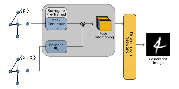
Figure 1: The proposed pipeline. In grey, we have the network that generates the conditioning input. The mask-generating network is the only section that gets pre-trained on surrogate masks. The downstream model, in yellow, can be any trainable generative model able to accept a 3-d tensor as conditioning input. The whole pipeline can be trained end-to-end.

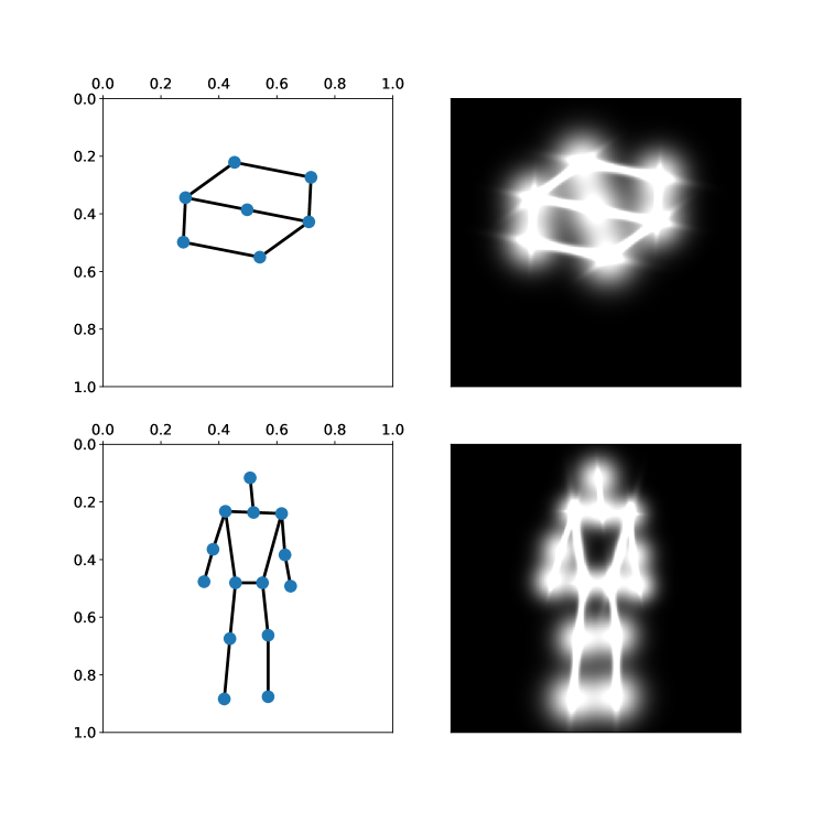
Figure 2: Examples of surrogate masks for a random graph (top) and for a graph representing a person (bottom). The position of a node in graph space is normalized between $0$ and $1$.

In this Section, we first provide a high-level description of our method, consequently propose an architecture implementing the framework and finally present our surrogate pre-training objective. Section 5 then empirically validates the proposed design.

3.1 Overview

Figure 1 provides an high-level view of our approach. Given an input pose graph ${\mathcal{G}}$, we wish to output a multi-channel mask ${\bm{\mathsfit{L}}}\in\left[0,1\right]^{C\times H\times W}$, which will then be used to condition the downstream model on a target generative task. We design the mask generation process so that the final mask is obtained by aggregating masks localized w.r.t. each node. In particular, we decompose the generation of ${\bm{\mathsfit{L}}}$ into the generation of a mask ${\bm{M}}_{i}\in\left[0,1\right]^{H\times W}$ and a feature vector ${\bm{f}}_{i}\in\left[0,1\right]^{C}$ for each node ${\bm{v}}_{i}$, such that:

$${\bm{\mathsfit{L}}}=\frac{1}{|{\mathcal{V}}|}\sum_{i\in{\mathcal{V}}}{\bm{f}}_{i}\otimes{\bm{M}}_{i},$$ (1)

where $\otimes$ indicates the tensor product. Notably, we make each ${\bm{M}}_{i}$ dependant on pose attributes ${\bm{P}}$ only, while features ${\bm{f}}$ depend on both pose and attributes $\left({\bm{P}}\|{\bm{X}}\right)$, so that the former encodes only structural information, while the latter will also eventually account for style. In particular, we compute both ${\bm{f}}_{i}$ and ${\bm{M}}_{i}$ by means of two learnable functions, such that our generative model can be summarized as:

$$\begin{split}{\bm{F}}&=\Phi_{\phi}\left({\bm{V}},{\bm{A}}\right)\\ {\bm{\mathsfit{M}}}&=\mu_{\theta}\left({\bm{P}},{\bm{A}}\right)\\ {\bm{\mathsfit{L}}}&=\frac{1}{|{\mathcal{V}}|}\sum_{i\in{\mathcal{V}}}{\bm{f}}_{i}\otimes{\bm{M}}_{i}\end{split}$$ (2)

Where ${\bm{\mathsfit{M}}}$ indicates the tensor encompassing all the ${\bm{M}}_{i}$ masks. The $\Phi_{\phi}$ function can be learned end-to-end with the downstream model, as shown in Section 5.2. Differently, we pre-train $\mu_{\theta}$ on a surrogate task designed to foster the learning of masks coherent with the structure of the object being generated. After pre-training, $\mu_{\theta}$ can be fine-tuned end-to-end with the downstream model on the target task. This approach is suitable for flexibly conditioning the generation on different tasks based on the structure of the objects. Notably, we implement our method with two neural networks that work in parallel: the Encoder ($\Phi_{\phi}$) and the Mask Generator ($\mu_{\theta}$). The former implements function $\Phi_{\phi}$ from Equation (2), while the latter implements function $\mu_{\theta}$. The outputs of the two networks are combined to obtain pose conditioning feature maps.

3.2 Implementing the encoder $\Phi_{\phi}$

The Encoder ($\Phi_{\phi}$) network is based on what we call a PoseConvolution layer, which consists of the following message-passing operator:

$${\bm{h}}_{i}^{\prime}=g_{g}\left(g_{s}\left({\bm{h}}_{i},{\bm{p}}_{i}\right)+\sum_{j\in\mathcal{N}\left(i\right)}g_{l}\left({\bm{h}}_{j},{\bm{p}}_{j}-{\bm{p}}_{i}\right),{\bm{h}}_{i}\right)$$ (3)

where $\mathcal{N}\left(i\right)$ is the set of neighbours of the $i$-th node, while $g_{s}$, $g_{l}$ and $g_{g}$ can be any learnable function (e.g., MLPs). Consistently with the previous naming convention, ${\bm{h}}_{i}$ and ${\bm{p}}_{i}$ indicate node features and position respectively. The layer is inspired by PointNet [11] but uses two distinct functions for processing the representation of the central node and computing messages coming from neighbors. In particular, $g_{s}$ can be seen as implementing a parametrized skip connection to mitigate over-smoothing node representations [12]. The final node encodings are obtained by stacking blocks of the form

$${\mathcal{G}}_{{\bm{H}}^{\prime}\|{\bm{P}}}=\textsc{BN}\left(\textsc{ReLU}\left(\textsc{PConv}\left({\mathcal{G}}_{{\bm{H}}\|{\bm{P}}}\right)\right)\right),$$ (4)

where BN denotes Batch Normalization [13], ReLU is the activation function,PConv is our PoseConvolution layer and ${\mathcal{G}}_{{\bm{H}}\|{\bm{P}}}$ a pose graph with features ${\bm{H}}$ and node coordinates ${\bm{P}}$.

3.3 Implementing the mask generator $\mu_{\theta}$

The Mask Generator ($\mu_{\theta}$) network consists of a first block of stacked Pose Convolutional layers analogous to the ones in Equation (4). The outputs of these layers are then reshaped into bi-dimensional matrices used as input for the second stack of layers consisting of a combination of convolution blocks (like those used in BigGan’s generator network [14]), interleaved with PoseConvolution2D layers. Such layers implement the following message-passing layer:

$$\begin{split}{\bm{O}}_{i}&=\sum_{j\in\mathcal{N}\left(i\right)}g_{o}\left({\bm{H}}_{i},{\bm{H}}_{j}\right)\\ {\bm{H}}_{i}^{\prime}&=g_{s}\left({\bm{H}}_{i}\right)+\sigma\left({\bm{O}}_{i}\right)\odot g_{g}\left({\bm{O}}_{i}\right)\end{split}$$ (5)

where, $\odot$ denotes the Hadamard product, $\mathcal{N}\left(i\right)$ is the set of neighbors of node $i$ and $g_{s}$, $g_{l}$ and $g_{g}$ can be any learnable function that has two-dimensional inputs and outputs.

In our case, $g_{g}$ is a 2D convolutional layer while $g_{o}$ is the previously mentioned BigGan’s generator block and $g_{s}$ is a linear upsampling operation followed by a 2D convolution, where the upsampling is needed to match the dimensions of the output of the $g_{o}$. The rationale behind the design of Equation (5) is promoting heterogeneity between the masks generated by different nodes by exploiting gating and skip connections. Notably, $g_{s}$ can act as skip connection preserving the node representation while the gating operation allows for selectively aggregating information coming for the neighbors. Indeed, over-smoothing the node features would be particularly detrimental in this case as it would compromise the locality of the masks learned w.r.t. each node. Said property is desirable as, per Equation (1) this would in turn make the learned node embeddings localized w.r.t. their neighborhood. Note that these soft constraints, i.e., architectural biases, can be seen as a form of regularization aligned with object-centric generation tasks.

3.4 Surrogate Task

As mentioned previously, we want to pre-train $\mu_{\theta}$ on the generic surrogate task of mapping a pose graph to a 2D mask. For this purpose, we define a surrogate mask associated with a graph ${\mathcal{G}}$, as shown in Figure 2, which, intuitively, is a grayscale image that depicts the structure of the graph.

The mask for the whole graph is obtained by composing partial masks relative to each node and edge. In particular, given pixel coordinates $c$, we define the value of the partial surrogate mask associated with the $i$-th node, at that pixel, as

$$\textsc{S}_{{\bm{N}},i}\left({\bm{c}}\right)=\exp\left(-\frac{\left\|{\bm{p}}_{i}-{\bm{c}}\right\|_{2}^{2}}{2\sigma^{2}}\right)$$ (6)

and, analogously, the value of the partial surrogate mask associated with edge $e_{ij}$ as

$$\textsc{S}_{{\bm{E}},ij}\left({\bm{c}}\right)=\sqrt{\frac{\exp\left(-d_{ij}({\bm{c}})^{T}\cdot{\bm{T}}_{ij}^{-1}\cdot d_{ij}({\bm{c}})\right)}{\left(2\pi\right)^{2}\cdot\det\left({\bm{T}}_{ij}\right)}},$$ (7)

where ${\bm{T}}_{ij}$ denotes a $2\times 2$ rotation and scaling matrix dependent on the length and angle of the segment connecting nodes $i$ and $j$ (see the supplementary material for the details); conversely, $d_{ij}({\bm{c}})$ is defined as

$$d_{ij}({\bm{c}})={\bm{c}}-\left(\frac{{\bm{p}}_{i}+{\bm{p}}_{j}}{2}\right)$$ (8)

and denotes the distance between ${\bm{c}}$ and the midpoint between the coordinates of nodes $i$ and $j$.

The value associated with pixel ${\bm{c}}$ of the final surrogate mask for ${\mathcal{G}}$ is then obtained as

$$\textsc{S}_{{\mathcal{G}}}\left({\bm{c}}\right)=\sum_{i\in{\mathcal{G}}}\textsc{S}_{{\bm{N}},i}\left({\bm{c}}\right)+\sum_{\langle i,j\rangle\in{\mathcal{G}}}\textsc{S}_{{\bm{E}},i,j}\left({\bm{c}}\right)$$ (9)

which is the pixel-wise sum of the masks associated with each node and edge. All the values are then clipped between $0$ and $1$. More details about the computation of the mask can be found in Appendix A.3. Intuitively, the mask corresponding to a node is obtained by considering an isotropic bi-variate Gaussian with mean equal to the node coordinate and standard deviation $\sigma$, over a discrete grid with the same size as the image we wish to generate. The mask corresponding to an edge, instead, is obtained by considering a bi-variate Gaussian with mean equal to the middle point between the two nodes connected by the edge, and covariance matrix dependent on the distance between the two points and the orientation of the line joining them. The surrogate mask obtained in such a way is agnostic w.r.t. the object represented by the graph and hence general. Note that differently from, e.g., segmentation masks, the mask we are referring to depends entirely on the structure of the objects in the image being generated, which can, in principle, vary in terms of style, structure, and class.

As a final remark, the surrogate mask has a lattice structure, which may not properly resemble the desired mask for all target tasks; indeed, depending on the specific object, some loops should be filled, or some parts should have peculiarly shaped features (e.g., four nodes forming a box or the nodes corresponding to hands in a human skeleton). Nonetheless, such surrogate masks are helpful in providing supervision for the pre-training routine and act as a regularization for the model. Details on the fine-tuning procedure on downstream tasks are discussed in Section 5.3. The pre-training routine is carried out by minimizing a surrogate loss $\mathcal{L}_{re}$ based on a reconstruction error, e.g., mean squared error or binary cross entropy.

4 Related Works

Image generation is a popular application of deep learning models from Generative Adversarial Networks (GANs) [15], to Variational Autoencoders (VAEs) [16] and, more recently, Diffusion Models [17, 18, 19]. Concurrently, many researchers have explored ways of conditioning the generation of such images, from simple class labels [20, 14], to fully articulated sentences [21, 22] or even other images [23, 24, 25]. Although no previous work directly exploits pose graphs to guide image generation, several approaches focused on Scene-Graph-Conditioned Image Generation and Pose-Conditioned Image Generation.

Scene-Graph-Conditioned Image Generation

Scene graphs are a way of representing a visual scene context as a graph linking object nodes through predicate edges. The first work that proposes image generation conditioned on a particular scene graph was written by Johnson et al. [1]. In their work they propose a GNN that maps the scene graph into a scene layout, that is then used to bias a generator network. Ivgi et al. [2], improved the first approach by using a GNN that directly works on 2D feature maps. Differently from the above, however, our work focuses on representing a specific object and its structure in space through a graph, rather than multiple abstract objects and their relationship without any geometrical constraint.

Pose-Conditioned Image Generation

Other prior works that we deem related to ours are concerned with pose-guided image generation. In particular, this niche deals with human image generation. The first deep learning approach to generate a person image conditioned on a particular pose and reference image was proposed by Ma et al. [3]. Others built on this approach using deformable convolutions [4], dense poses [5] or explicit attributes [26]. A typical problem solved by these techniques is person re-identification [6]. The work by Horiuchi et al. [27], instead, implicitly uses a graph-based representation for the pose and a reference image for semantics. The main difference with our approach is that we jointly encode pose and semantics in a graph. This makes the conditioning more flexible and unties it from a pre-existing person image composed of a specific set of properties that are difficult to modify indiependently.

5 Experiments

This section reports the results obtained by applying our method. In particular, we first show our results in pre-training the mask generator $\mu_{\theta}$ with surrogate masks created from random graphs. Finally, we present an application to image generation conditioned on human poses and compare our approach against relevant baselines. The code used to run the experiments is provided in the supplementary materials.

5.1 Surrogate Pre-Training

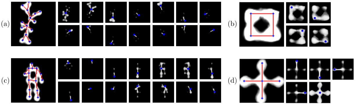
Figure 3: Examples of masks generated from different graphs. For each sample, the larger figure shows the aggregated mask, while the smaller ones those of each specific node. The blue dots highlight the position of the node being considered. Samples (b) and (d) are simple handcrafted graphs. Sample (a) is an example of a random graph like those in the pre-training routine. Sample (c) is a human pose graph.

For surrogate pre-training, we generate random graphs using a Barbasi-Albert model [28], with number of nodes uniformly sampled in the interval $\left[5,30\right]$; number of edges for new nodes is set to $1$ in $90\%$ of the cases and to $2$ in the remaining $10\%$. These parameters are chosen as to generate graphs simple to be drawn on the plane, i.e., with only a few intersections among edges. The position of each node is determined by using Kamada-Kawai’s force-directed graph drawing algorithm [29]. While alternatives exist, and even random placing is a possible choice, the Kamada-Kawai’s algorithm creates structures that mostly avoid edge overlaps for a wide range of node counts. Objective masks are computed as in Equation (9) and the model is fitted to minimize the Binary Cross Entropy (BCE) loss. Figure 3 shows sample results for the mask generation. Each of the bigger images corresponds to the full mask generated from the input graph superimposed in blue (nodes) and red (edges), while the smaller images are the masks relative to each node (superimposed in blue). The model is able to produce masks that match the topology of the graph, even for complex structures. More interestingly, results show that the proposed architecture is indeed capable of generating node-level masks that capture the structure of the neighbourhood of each node. By looking at samples (b) and (d), which contain handcrafted graphs, we see that this property is preserved for graphs with a small diameter; even though, nodes with high connectivity tend to produce richer masks that may span it completely. Indeed, locality is preserved against over-smoothing which is typical of isotropic graph convolutional filters; conversely, the learned node-level masks are diverse and properly localized.

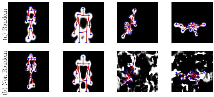
Figure 4: Examples of masks generated by pre-training on random graphs (a) and on graphs from the downstream task (b). First two columns are graphs from the downstream task, while the last two are random graphs. In (b), performance clearly degrades out of distribution.

In Figure 4, we additionally show how pre-training on randomly generated graphs act as regularization by yielding a model able to perform properly for graphs outside the distribution of the downstream task,

5.2 Application

Model	FID $\downarrow$	# Train Params	# Inference Params
BigGAN	91.71	9.77 M	4.89 M
Baseline	57.71	13.82 M	8.57 M
GraPhOSE	46.97	14.15 M	8.87 M
No Pretrain	74.63	14.15 M	8.87 M

Table 1: Frechet Inception Distance (FID) score (lower is better) and parameters counts. Note that at inference time the discriminator model is not needed.

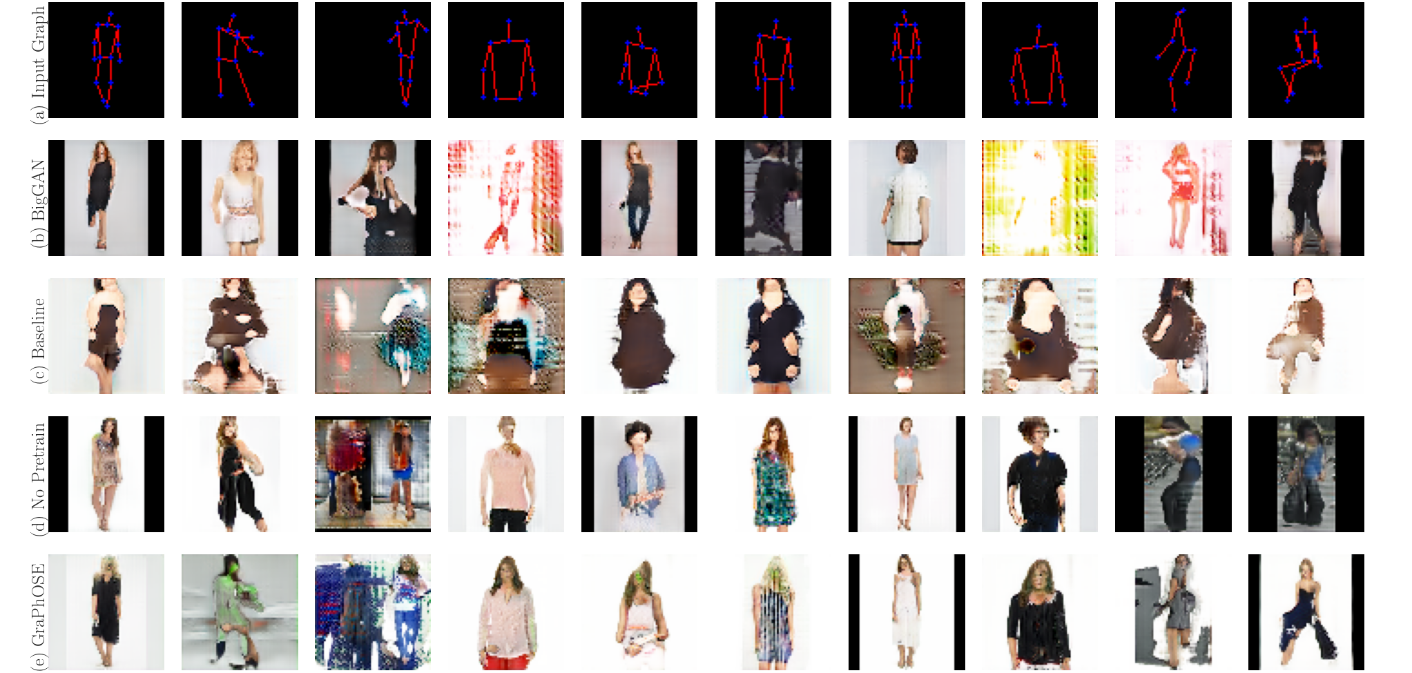
Figure 5: Random sample of images generated by GraPhOSE (e), GraPhOSE without surrogate mask pre-training (d), baseline without explicit relational structure (c), BigGAN without conditioning (b). The first row (a) shows the pose graph used for conditioning.

As an example of downstream task for which our methodology can be used, we choose that of person image generation conditioned on a specific pose and keypoint IDs as attributes. We use BigGan [14] as downstream model, slightly modified to receive as input our conditioning as a multi-channel mask. Moreover, similarly to [1], each stage of the generator takes as input both the previous stage’s output and a properly downsampled version of the multi-channel conditioning mask to guide generation at different scales. The original discriminator is also modified to receive the graph as input, together with the real/fake image; further details are provided in Appendix A.4. Note that, during the end-to-end training, we drop the reconstruction loss originally used to pre-train the mask generator. This is to allow for adapting to the downstream task, without the bias coming from the surrogate loss. We pre-train the mask generator as described in Section 5.1, and the whole pipeline is trained on data coming from three different datasets: MPII Human Pose Dataset [30], Market 1501 [31] and DeepFashion [32]. For the DeepFashion dataset we use just the Fashion Landmark Detection and the In-Shop Retrieval subsets. The keypoint annotations for DeepFashion In-Shop Retreival and Market 1501 are based on [33], and were generated by using the open-source software OpenPose [34]. For DeepFashion Fashion Landmark we instead rely on MediaPipe’s BlazePose [35], while MPII Human Pose already contains pose features. All annotations are reduced to the COCO Keypoint standard [36] and used to generate the corresponding graphs with node coordinates normalized between $0$ and $1$. Images are resized, and zero-padded when needed, to a $64\times 64$ shape.

We compare the results obtained by our model against two different baselines. The first one is a standard BigGan, analogous to the one modified to use as a downstream model for our pipeline; this baseline is to assess the quality achievable by a model without any conditioning. The other baseline is, instead, a non-relational model: if we consider Equation (2), we can describe it in an analogous way as

$$\begin{split}{\bm{F}}&=\Psi{\psi}\left({\bm{V}}\right)\\ {\bm{\mathsfit{M}}}&=\operatorname*{\mathchoice{\Bigg{\|}}{\Big{\|}}{\|}{\|}}_{i\in{\mathcal{V}}}\left(\textsc{S}_{{\bm{N}},i}\left({\bm{C}}\right)+\sum_{j\in{\mathcal{N}}(i)}\textsc{S}_{{\bm{E}},ij}\left({\bm{C}}\right)\right)\\ {\bm{\mathsfit{L}}}&=\frac{1}{|{\mathcal{V}}|}\sum_{i\in{\mathcal{V}}}{\bm{f}}_{i}\otimes{\bm{M}}_{i},\end{split}$$ (10)

where $\operatorname*{\mathchoice{\Bigg{\|}}{\Big{\|}}{\|}{\|}}_{i\in{\mathcal{V}}}$ indicates concatenation along a new axis, while, for ease of notation, $\textsc{S}_{{\bm{N}},i}\left({\bm{C}}\right)$ and $\textsc{S}_{{\bm{E}},ij}\left({\bm{C}}\right)$ denote the respective operations applied over all the pixel coordinates. In particular, in Equation (10), ${\bm{\mathsfit{M}}}$ is computed by means of a fixed (non-trainable) function, leveraging the procedure used for creating surrogate masks. $\Psi_{\psi}$ instead denotes a learnable function that is shared across all nodes and does not consider relational information (i.e., the adjacency matrix); it is implemented by means of a network analogous to the encoder used in the relational model, minus the message passing. The objective, in this case, is to compare against a model that does not account for the graph structure within the processing architecture, while still maintaining a similar design with conditioning on a hand-crafted mask. See Appendix A.5 for a detailed description of the baselines. All models were trained under the same settings; more details can be found in Appendix A.2.

Table 1 shows the Frechet Inception Distance (FID) score [37] for our model and the baselines we wish to compare it to. GraPhOSE achieves a better score when compared to the non-relational baseline, and results suggest that the surrogate mask pre-training plays a relevant role in achieving these results given an equivalent training setting. In fact, the model without pre-training performs worse than the one with pre-training and even worse than the vanilla BigGan baseline. Finally, we comment that the downstream model on its own has worse performance than that of models with a conditioning on the generative process. However, it is worth noting that FID accounts for the overall similarity between the distribution of images in the dataset and the one generated by the models; indeed, FID does not account for the position of the objects in the generated images. We assess this property visually, in a qualitative manner.

In this regard, Figure 5, shows results generated by BigGAN, the non-relational baseline and GraPhOSE, for a random sample from our validation set. For images generated by BigGAN, row (b), the pose graph bears no meaning, as the model is not conditioned on it, but they give a visual cue on how the images generated from our model have similar quality w.r.t. the ones generated by the downstream model. For GraPhOSE, row (e), the overall pose and scale of the person in the generated image comply with the input graph, even though specific details might be missing, e.g., for complex poses. However, this is also likely to be a bias coming from the training data, in which simple standing poses are more frequent. Moreover, training at a higher resolution might improve the generation of fine-grained details, e.g., hands, that in $64\times 64$ images occupy a very limited amount of pixels.

The images generated by training GraPhOSE without pre-training on surrogate masks, row (d), are still consistent with the input pose, even though, as shown in Figure 6, the intermediate masks ${\bm{M}}_{i}$, generated in such setting, do not visually resemble the persons’ pose. The lack of structure in the mask leads to degradation of the performance, in particular for uncommon poses, as results suggest. Note that, even without pre-training, the model still leverages the relational biases encoded in the graph, although not in the way our design intended, which benefits from localized masks. This shows the usefulness of pre-training as a soft regularization, which localizes node features w.r.t. corresponding portions of the image. Finally, by looking at the images generated by the non-relational baseline, row (c), it is possible to notice a generally worse visual appeal, with skin tones placed inconsistently across the figure; even though the FID score was comparable to that of the other models. The pose is somewhat respected, but the relational representation plays nonetheless a significant role in guiding the generation toward a coherent result.

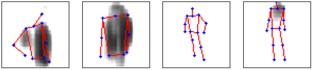
Figure 6: Samples of masks generated by GraPhOSE’s mask generator after end-to-end training without surrogate mask pre-training. The input graph is superimposed in blue (nodes) and red (edges).

5.3 Task specific mask adaptation

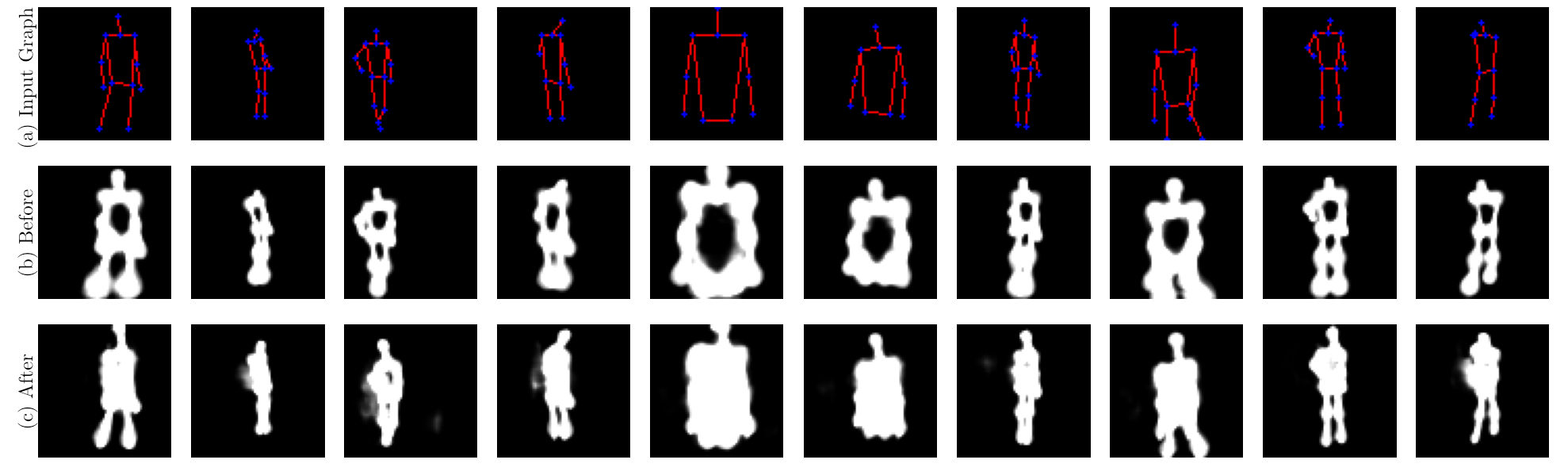
Figure 7: Random sample of masks generated by our model before the end-to-end training on the downstream task (b) and after (c). The top row (a) shows the corresponding input graph. Row (b) shows masks after pre-training (no fine-tuning).

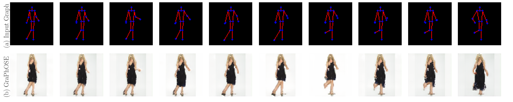
Figure 8: Row (b) shows the results obtained by fixing all inputs to our model and just changing the attributes describing the position of some nodes. The top row (a) is the corresponding input graph pose.

The purpose of pre-training on surrogate masks of random pose graphs is to learn a general mapping between the graph and the image representation of the structure it entails. However, this learned mapping might not produce the exact visual properties desirable for a specific downstream task. We wish to adapt to these properties while learning the target task, during the end-to-end training. Figure 7 shows changes in the masks being generated before and after training on the target task, given the same input. We can notice how the model learned that the torso section needs to be filled, that the legs should be thinner, and that the head is composed of a slim section and a round part. This result is particularly relevant, as it shows that after a pre-training that pushes the mask generator in the correct direction, it is then possible to have it learn the specifics on the target downstream task.

5.4 Pose Manipulation

To assess whether the model is able to disentangle pose attributes and style, we experiment with providing it with a series of input graphs with slightly different limb positions, while maintaining all other inputs fixed. As shown in Figure 8, generated figure moves are rearranged according to the changes in the input pose while the style is mostly unchanged. Note that, however, in case of more significant changes in the pose, the resulting images were visually different. This emergent property is nonetheless interesting and provides ground for future research.

6 Conclusions and Future Work

We propose GraPhOSE, a method to exploit attributed graphs as object-centric relational inductive biases to flexibly condition image generation. Our approach has several advantages compared to standard approaches which result in a scalable and flexible framework. Notably, we shone a light on the properties of relational representation in this context, by showing how they can be used to regularize and manipulate the generative model. Future research could investigate different approaches to generate meaningful and coherent masks without pre-training and investigate methods to further disentangle the different elements that contribute to the final generated image. We argue that our study has the potential of sparking new interest in object-centric relational inductive biases for generative modeling and that the results presented here constitute the first building block for future research in this direction.

Appendix A Implementation Details

In the following we clarify some details on the settings used to train the models, on the specifics of some models’ architectures, as well as further details on surrogate masks and the hardware and software we used to run the experiments.

A.1 Hardware and Software

The code to run the experiments is all written in Python 3.9, leveraging Pytorch [38] and Pytorch Lightning [39] to define models and data, while Hydra [40] is used to manage the experiment configuration. Weights & Biases [41] is used to log and compare experiment results. We run all the experiments on an NVIDIA RTX A5000 GPU equipped with 24GBs of VRAM. All code will be made open-source through GitHub upon publication.

A.2 Training settings

Each model is trained under the same settings, chosen based on those used originally to train BigGAN [14]. In particular, we use the Adam [42] optimizer, with Cosine Annealing [43] learning rate schedule with period $150$, starting learning rate $0.002$ and final learning rate $0.00002$. Models are trained for $150$ epochs each, with a batch size of $64$. Notice that the learning rate for the parameters of the pre-trained mask generator used in GraPhOSE was 100 times smaller with respect to the learning rate of the other parameters, in order to avoid catastrophic foregetting at the beginning of training. This procedure could be enhanced by slowly raising the learning rate of the pre-trained parameters back to the value of other parameters, as training epochs go by, with the aim of favoring mask adaptation after the training has stabilized during the first epochs.

A.3 Surrogate Mask

Referring to Equation (7), we explicitly define ${\bm{T}}_{ij}$ as

$$\begin{split}d_{ij}&=\frac{\|{\bm{p}}_{i}-{\bm{p}}_{j}\|^{2}_{2}}{4}\\ \alpha_{ij}&=\arctan 2\left({\bm{p}}_{j}-{\bm{p}}_{i}\right)\\ {t}_{a,ij}&=d_{ij}\cdot\cos\left(\alpha_{ij}\right)^{2}+\frac{d_{ij}}{a^{2}}\cdot\sin\left(\alpha_{ij}\right)^{2}\\ {t}_{b,ij}&=d_{ij}\cdot\sin\left(\alpha_{ij}\right)^{2}+\frac{d_{ij}}{a^{2}}\cdot\cos\left(\alpha_{ij}\right)^{2}\\ {t}_{c,ij}&=\left(d_{ij}-\frac{d_{ij}}{a^{2}}\right)\cdot\sin\left(\alpha_{ij}\right)\cdot\cos\left(\alpha_{ij}\right)\\ {\bm{T}}_{ij}&=\begin{bmatrix}{t}_{a,ij}&{t}_{c,ij}\\ {t}_{c,ij}&{t}_{b,ij}\end{bmatrix},\end{split}$$ (11)

where vectors ${\bm{p}}$ denote node coordinates, $\arctan 2$ is the element-wise 2-argument arctangent and $a$ denotes a parameter that regulates the scaling ratio of the second dimension w.r.t. the first one. In our experiments $a$ is set to $10$.

A.4 Changes to the downstream model

As mentioned in Section 5.2, we modify BigGAN’s generator and discriminator for our purposes; the former to accept our conditioning, the latter to take both an image and a graph as input. Regarding the generator, we simply concatenate our multi-channel conditioning mask to the optional 2D noise matrix that is originally the generator’s input. Furthermore, we modify its original convolution block to have the following form

$$\begin{split}{\bm{\mathsfit{H}}}^{\prime}&=\sigma\left(\textsc{Conv2D}\left(\textsc{Upsample}\left(\sigma\left({\bm{\mathsfit{H}}}\right)\right)\right)\right)\\ {\bm{\mathsfit{K}}}&=\textsc{Conv2D}\left(\textsc{AvgPool2D}\left({\bm{\mathsfit{L}}}\right)\right)\\ {\bm{\mathsfit{H}}}^{\prime\prime}&=\textsc{Conv2D}\left({\bm{\mathsfit{H}}}\right)+\textsc{Conv2D}\left({\bm{\mathsfit{H}}}^{\prime}\|{\bm{\mathsfit{K}}}\right),\end{split}$$ (12)

where ${\bm{\mathsfit{H}}}$ represents the input feature maps, while ${\bm{\mathsfit{L}}}$ is the conditioning multi-channel mask. Conv2D is a two-dimensional convolution layer, Upsample denotes a channel-wise times-two linear interpolation upsample operation and $\sigma$ is batch-normalization followed by a rectified linear unit. Lastly, AvgPool2D is a two-dimensional average pooling operation that matches the size of the last two dimensions of ${\bm{\mathsfit{L}}}$ to those of ${\bm{\mathsfit{H}}}^{\prime}$. ${\bm{\mathsfit{H}}}^{\prime\prime}$ is the output of the convolution block.

Regarding the discriminator, instead, we add a graph encoder with the same network architecture used to implement $\Phi_{\phi}$ in Equation (2). The output of this encoder is then concatenated to the feature vector extracted from the input image by the discriminator’s original image encoder. The resulting vector goes through a linear layer, a ReLU and another linear layer, as in the original BigGAN’s discriminator. This final output is then used to compute the adversarial loss. Note that our additional graph encoder does not change the discriminator’s original design.

A.5 Non-relational Baseline architecture

The non-relational baseline model architecture follows the same structure of our GraPhOSE model, with the main difference that, instead of graph convolutions, it uses only shared linear layers to compute $\Psi_{\psi}$, in Equation (10). In particular, we keep the same architecture used for GraPhOSE, made of layers of the form shown in Equation (4), where, instead of PConv layers, we have the following operator

$${\bm{h}}_{i}^{\prime}=g\left({\bm{h}}_{i},{\bm{p}}_{i}\right),$$ (13)

where ${\bm{h}}_{i}$ are node features and ${\bm{p}}_{i}$ denotes node positions. In our case $g$ is a linear layer. Node masks ${\bm{M}}_{i}$ are computed as shown in Equation (10). The rest of the generator is the same as the one used by our model. The discriminator for the baseline extracts features from the input graph following the same principle described in Appendix A.4, with the only difference that the features are extracted using $\Psi_{\psi}$ instead of $\Phi_{\phi}$. Note that this model has no access to explicit relational information regarding how the key points are connected together, even though this information is implicitly provided through the non-learnable masks, as it is still necessary to have a meaningful comparison with our model.

Appendix B Other experiments

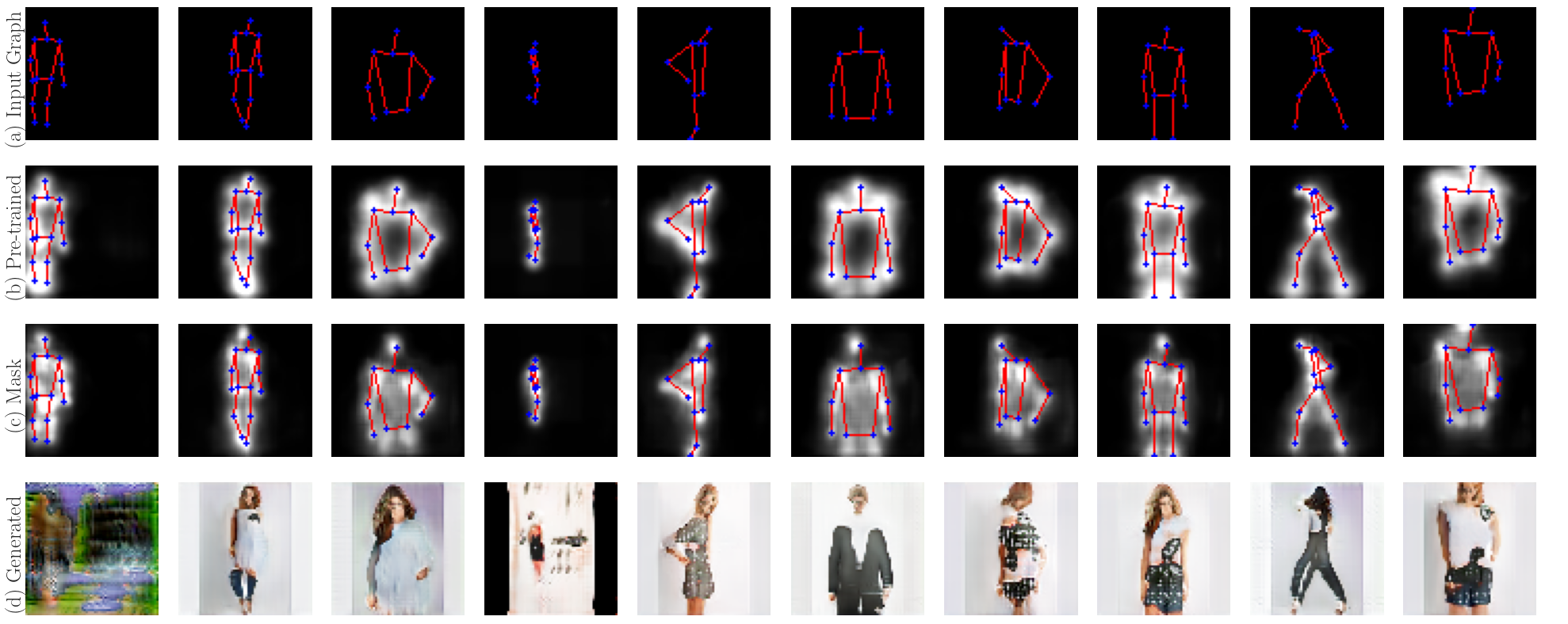
Figure 9: Examples of images (d) and masks (c) generated by training GraPhOSE with a mask generator pre-trained on the MSE loss function. Row (a) shows the input graph, while row (b) shows the masks generated by the pre-trained mask generator, before end-to-end training.

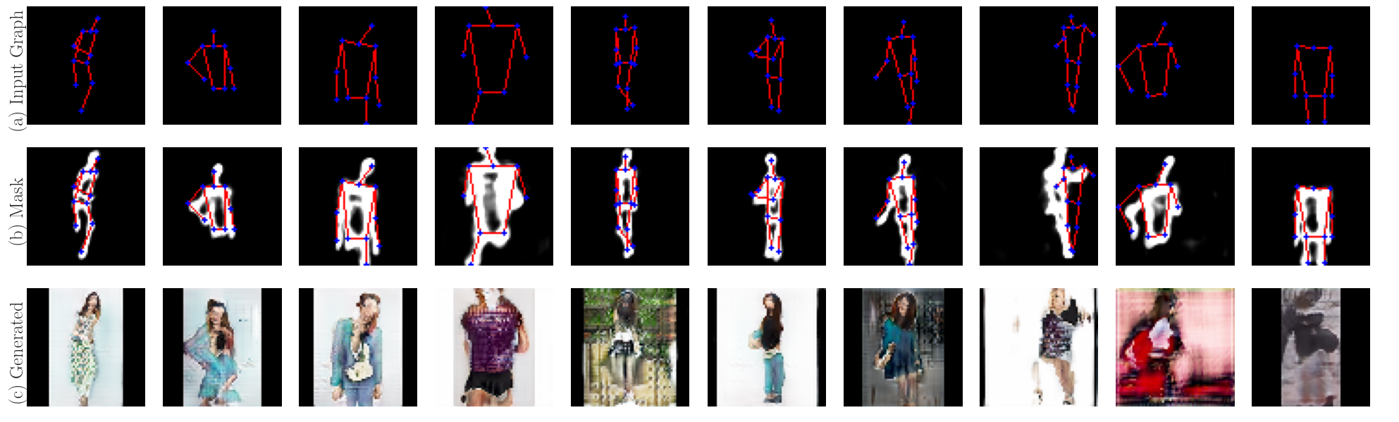
Figure 10: Examples of images (c) and masks (b) generated by training GraPhOSE with a discriminator that does not take the graph as input. Row (a) shows the input graph.

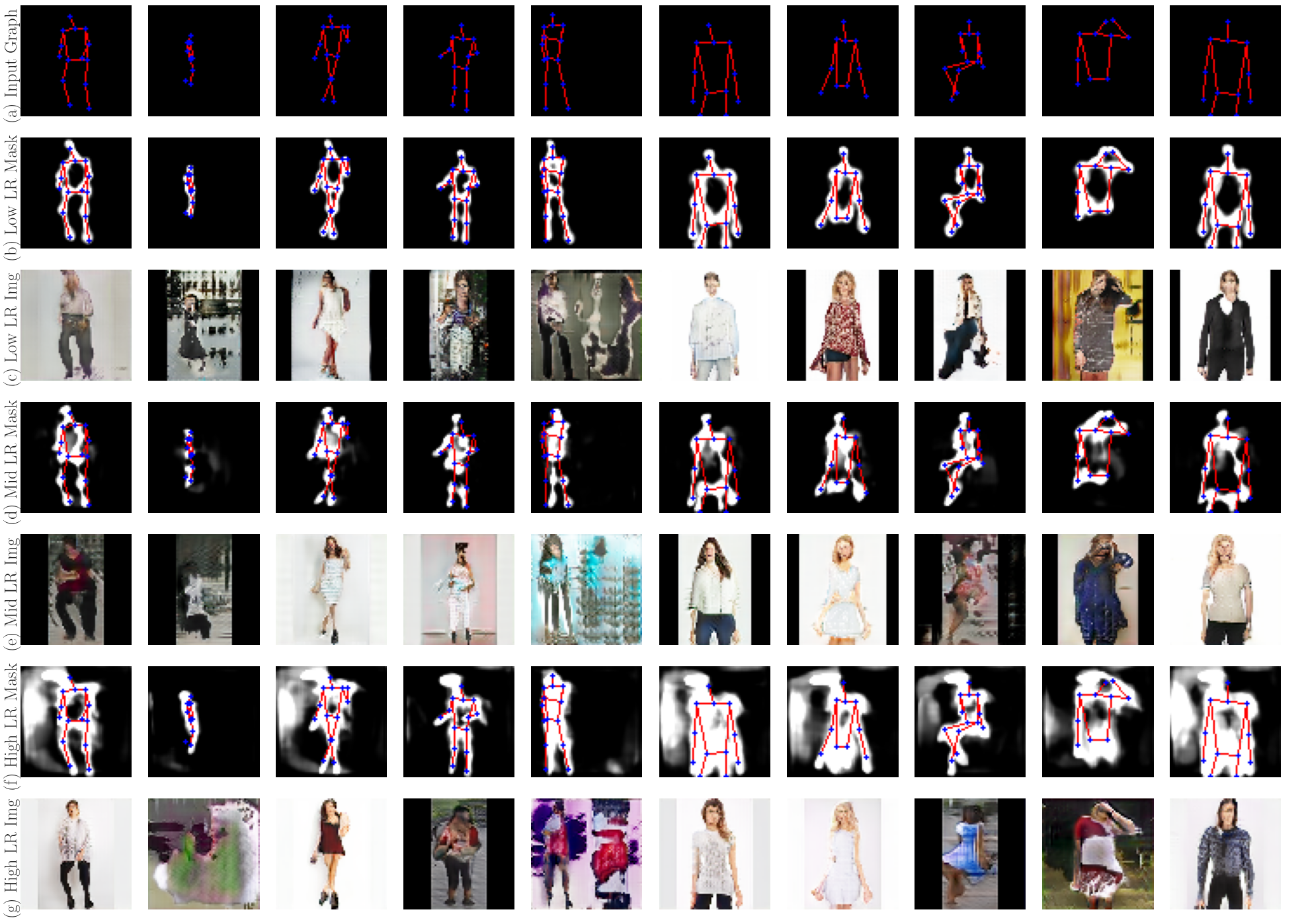
Figure 11: Examples of images and masks generated by training GraPhOSE with different learning rates for the pre-trained parameters. Row (a) shows the input graph. Rows (b) and (c) show, respectively, the masks and images obtained with the lowest learning rate used. Equivalently, rows (d) and (e), and rows (f) and (g), show those obtained by using a middle ground learning rate and an higher one respectively.

Here is a collection of result images generated by training models with slight architectural changes. We deemed these changes to not affect the results sufficiently or clearly enough to be part of an interesting discussion, but we still provide them for completeness and for interested readers.

B.1 MSE pre-trained Mask Generator

We experiment with using the Mean Square Error (MSE) as loss function for the mask reconstruction during pre-training. Figure 9 shows a sample of the results we achieved. The most evident characteristic of the masks produced with these settings is that they appear softer than those produced by using a BCE loss. This is likely due to the structure of the losses themselves; nonetheless we can see that the softer conditioning is still able to produce good results on average, while possibly being more prone to forgetting during end-to-end training.

B.2 Image-only Discriminator

Figure 10 shows a sample of the results obtained by training GraPhOSE with the standard BigGAN’s discriminator, which does not take the graph as input, but only the real/fake image. It is noticeable how the input pose is mostly respected, however, the model is more susceptible to failure when receiving uncommon poses. The generated masks, on row (b), are more detached from the input graph’s pose; this is most likely due to the fact that, as the discriminator cannot leverage information about the conditioning, it cannot effectively recognize as fake, images with good visuals but incorrect poses. This, in turn, provides a less useful adversarial training cycle, and we could expect that, with an higher learning rate on the mask generator, or more training epochs, the pre-learned function could be completely forgotten.

B.3 Varying learning rate reduction factor

As already mentioned in Section A.2, we applied a reduction factor to the learning rate of the pre-trained parameters, in order to avoid catastrophic forgetting during the early training steps. Here we show the results obtained by using a smaller reduction factor, hence an higher learning rate, for such parameters.

Model	LR Reduction Factor	FID $\downarrow$
Low LR	0.01	50.69
Mid LR	0.05	57.13
High LR	0.1	54.86

Table 2: Frechet Inception Distance (FID) score (lower is better) for different learning rate reduction factors on the pre-trained parameters.

The FID scores, reported in Table 2, show that, given otherwise equal training conditions, the highest reduction, hence the lower learning rate, provides the best results. However, the difference is rather small, which points towards the fact that some more advanced learning rate scheduling might be used to provide stability during the first epochs and more adaptability during the later ones.

By looking at the results shown in Figure 11, we can see how, on average, we reach good results for all the three settings of the pre-trained parameters learning rate. Noticeably, the characteristics of the generated masks vary strongly as the learning rate is increased, which, as mentioned, is a thing we might wish for the later stages of training, in order to better conform to the specifics of the downstream task. Another thing worth noting is that, for the highest learning rate setting, the masks start to contain patches outside of the object’s outline. This suggest the model is trying to condition the background, which in principle could be useful. Further exploration of this behavior may suggest a design in which an additional entity is added to the relational structure to account for the general conditioning of the background and a more complex learning rate scheduling is used. .

References

- Johnson et al. [2018] J. Johnson, A. Gupta, and L. Fei-Fei, “Image Generation from Scene Graphs,” arXiv:1804.01622 [cs], Apr. 2018, arXiv: 1804.01622. [Online]. Available: http://arxiv.org/abs/1804.01622
- Ivgi et al. [2021] M. Ivgi, Y. Benny, A. Ben-David, J. Berant, and L. Wolf, “Scene Graph to Image Generation with Contextualized Object Layout Refinement,” arXiv, Tech. Rep. arXiv:2009.10939, Jul. 2021, arXiv:2009.10939 [cs] type: article. [Online]. Available: http://arxiv.org/abs/2009.10939
- Ma et al. [2017] L. Ma, X. Jia, Q. Sun, B. Schiele, T. Tuytelaars, and L. Van Gool, “Pose guided person image generation,” Advances in neural information processing systems, vol. 30, 2017.
- Siarohin et al. [2018] A. Siarohin, E. Sangineto, S. Lathuiliere, and N. Sebe, “Deformable gans for pose-based human image generation,” in Proceedings of the IEEE conference on computer vision and pattern recognition, 2018, pp. 3408–3416.
- Neverova et al. [2018] N. Neverova, R. A. Guler, and I. Kokkinos, “Dense pose transfer,” in Proceedings of the European conference on computer vision (ECCV), 2018, pp. 123–138.
- Qian et al. [2018] X. Qian, Y. Fu, T. Xiang, W. Wang, J. Qiu, Y. Wu, Y.-G. Jiang, and X. Xue, “Pose-normalized image generation for person re-identification,” in Proceedings of the European conference on computer vision (ECCV), 2018, pp. 650–667.
- Jiang et al. [2022] Y. Jiang, S. Yang, H. Qju, W. Wu, C. C. Loy, and Z. Liu, “Text2human: Text-driven controllable human image generation,” ACM Transactions on Graphics (TOG), vol. 41, no. 4, pp. 1–11, 2022.
- Gilmer et al. [2017] J. Gilmer, S. S. Schoenholz, P. F. Riley, O. Vinyals, and G. E. Dahl, “Neural message passing for quantum chemistry,” in International conference on machine learning. PMLR, 2017, pp. 1263–1272.
- Bacciu et al. [2020] D. Bacciu, F. Errica, A. Micheli, and M. Podda, “A gentle introduction to deep learning for graphs,” Neural Networks, vol. 129, pp. 203–221, 2020.
- Bronstein et al. [2021] M. M. Bronstein, J. Bruna, T. Cohen, and P. Veličković, “Geometric deep learning: Grids, groups, graphs, geodesics, and gauges,” arXiv preprint arXiv:2104.13478, 2021.
- Qi et al. [2017] C. R. Qi, H. Su, K. Mo, and L. J. Guibas, “Pointnet: Deep learning on point sets for 3d classification and segmentation,” in Proceedings of the IEEE conference on computer vision and pattern recognition, 2017, pp. 652–660.
- Li et al. [2019] G. Li, M. Muller, A. Thabet, and B. Ghanem, “DeepGCNs: Can GCNs go as deep as CNNs?” in Proceedings of the IEEE/CVF international conference on computer vision, 2019, pp. 9267–9276.
- Ioffe and Szegedy [2015] S. Ioffe and C. Szegedy, “Batch normalization: Accelerating deep network training by reducing internal covariate shift,” in International conference on machine learning. PMLR, 2015, pp. 448–456.
- Brock et al. [2018] A. Brock, J. Donahue, and K. Simonyan, “Large scale gan training for high fidelity natural image synthesis,” arXiv preprint arXiv:1809.11096, 2018.
- Goodfellow et al. [2014] I. J. Goodfellow, J. Pouget-Abadie, M. Mirza, B. Xu, D. Warde-Farley, S. Ozair, A. C. Courville, and Y. Bengio, “Generative adversarial nets,” in NIPS, 2014.
- Kingma and Welling [2013] D. P. Kingma and M. Welling, “Auto-encoding variational bayes,” arXiv preprint arXiv:1312.6114, 2013.
- Sohl-Dickstein et al. [2015] J. Sohl-Dickstein, E. Weiss, N. Maheswaranathan, and S. Ganguli, “Deep unsupervised learning using nonequilibrium thermodynamics,” in International Conference on Machine Learning. PMLR, 2015, pp. 2256–2265.
- Song and Ermon [2019] Y. Song and S. Ermon, “Generative modeling by estimating gradients of the data distribution,” Advances in neural information processing systems, vol. 32, 2019.
- Ho et al. [2020] J. Ho, A. Jain, and P. Abbeel, “Denoising diffusion probabilistic models,” Advances in Neural Information Processing Systems, vol. 33, pp. 6840–6851, 2020.
- Mirza and Osindero [2014] M. Mirza and S. Osindero, “Conditional generative adversarial nets,” arXiv preprint arXiv:1411.1784, 2014.
- Ramesh et al. [2022] A. Ramesh, P. Dhariwal, A. Nichol, C. Chu, and M. Chen, “Hierarchical text-conditional image generation with clip latents,” arXiv preprint arXiv:2204.06125, 2022.
- Rombach et al. [2022] R. Rombach, A. Blattmann, D. Lorenz, P. Esser, and B. Ommer, “High-resolution image synthesis with latent diffusion models,” in Proceedings of the IEEE/CVF Conference on Computer Vision and Pattern Recognition, 2022, pp. 10 684–10 695.
- Isola et al. [2017] P. Isola, J.-Y. Zhu, T. Zhou, and A. A. Efros, “Image-to-image translation with conditional adversarial networks,” in Proceedings of the IEEE conference on computer vision and pattern recognition, 2017, pp. 1125–1134.
- Liu et al. [2017] M.-Y. Liu, T. Breuel, and J. Kautz, “Unsupervised image-to-image translation networks,” Advances in neural information processing systems, vol. 30, 2017.
- Zhu et al. [2017] J.-Y. Zhu, T. Park, P. Isola, and A. A. Efros, “Unpaired image-to-image translation using cycle-consistent adversarial networks,” in Computer Vision (ICCV), 2017 IEEE International Conference on, 2017.
- Men et al. [2020] Y. Men, Y. Mao, Y. Jiang, W.-Y. Ma, and Z. Lian, “Controllable person image synthesis with attribute-decomposed gan,” in Proceedings of the IEEE/CVF conference on computer vision and pattern recognition, 2020, pp. 5084–5093.
- Horiuchi et al. [2021] Y. Horiuchi, E. Simo-Serra, S. Iizuka, and H. Ishikawa, “Differentiable rendering-based pose-conditioned human image generation,” in Proceedings of the IEEE/CVF Conference on Computer Vision and Pattern Recognition, 2021, pp. 3921–3925.
- Albert and Barabási [2002] R. Albert and A.-L. Barabási, “Statistical mechanics of complex networks,” Reviews of modern physics, vol. 74, no. 1, p. 47, 2002.
- Kamada and Kawai [1989] T. Kamada and S. Kawai, “An algorithm for drawing general undirected graphs,” Information Processing Letters, vol. 31, no. 1, pp. 7–15, Apr. 1989. [Online]. Available: https://doi.org/10.1016/0020-0190(89)90102-6
- Andriluka et al. [2014] M. Andriluka, L. Pishchulin, P. Gehler, and B. Schiele, “2d human pose estimation: New benchmark and state of the art analysis,” in IEEE Conference on Computer Vision and Pattern Recognition (CVPR), June 2014.
- Zheng et al. [2015] L. Zheng, L. Shen, L. Tian, S. Wang, J. Wang, and Q. Tian, “Scalable person re-identification: A benchmark,” in Computer Vision, IEEE International Conference on, 2015.
- Liu et al. [2016] Z. Liu, P. Luo, S. Qiu, X. Wang, and X. Tang, “Deepfashion: Powering robust clothes recognition and retrieval with rich annotations,” in Proceedings of IEEE Conference on Computer Vision and Pattern Recognition (CVPR), June 2016.
- Zhu et al. [2019] Z. Zhu, T. Huang, B. Shi, M. Yu, B. Wang, and X. Bai, “Progressive pose attention transfer for person image generation,” arXiv preprint arXiv:1904.03349, 2019.
- Cao et al. [2019] Z. Cao, G. Hidalgo Martinez, T. Simon, S. Wei, and Y. A. Sheikh, “Openpose: Realtime multi-person 2d pose estimation using part affinity fields,” IEEE Transactions on Pattern Analysis and Machine Intelligence, 2019.
- Bazarevsky et al. [2020] V. Bazarevsky, I. Grishchenko, K. Raveendran, T. Zhu, F. Zhang, and M. Grundmann, “Blazepose: On-device real-time body pose tracking,” 2020. [Online]. Available: https://arxiv.org/abs/2006.10204
- Lin et al. [2014] T.-Y. Lin, M. Maire, S. Belongie, L. Bourdev, R. Girshick, J. Hays, P. Perona, D. Ramanan, C. L. Zitnick, and P. Dollár, “Microsoft coco: Common objects in context,” 2014. [Online]. Available: https://arxiv.org/abs/1405.0312
- Heusel et al. [2017] M. Heusel, H. Ramsauer, T. Unterthiner, B. Nessler, and S. Hochreiter, “Gans trained by a two time-scale update rule converge to a local nash equilibrium,” in Advances in Neural Information Processing Systems, I. Guyon, U. V. Luxburg, S. Bengio, H. Wallach, R. Fergus, S. Vishwanathan, and R. Garnett, Eds., vol. 30. Curran Associates, Inc., 2017. [Online]. Available: https://proceedings.neurips.cc/paper/2017/file/8a1d694707eb0fefe65871369074926d-Paper.pdf
- Paszke et al. [2019] A. Paszke, S. Gross, F. Massa, A. Lerer, J. Bradbury, G. Chanan, T. Killeen, Z. Lin, N. Gimelshein, L. Antiga et al., “Pytorch: An imperative style, high-performance deep learning library,” Advances in neural information processing systems, vol. 32, 2019.
- Falcon and team [2019] W. Falcon and T. P. L. team, “Pytorch lightning,” 3 2019. [Online]. Available: https://www.pytorchlightning.ai
- Yadan [2019] O. Yadan, “Hydra - a framework for elegantly configuring complex applications,” Github, 2019. [Online]. Available: https://github.com/facebookresearch/hydra
- Biewald [2020] L. Biewald, “Experiment tracking with weights and biases,” 2020, software available from wandb.com. [Online]. Available: https://www.wandb.com/
- Kingma and Ba [2014] D. P. Kingma and J. Ba, “Adam: A method for stochastic optimization,” arXiv preprint arXiv:1412.6980, 2014.
- Loshchilov and Hutter [2016] I. Loshchilov and F. Hutter, “Sgdr: Stochastic gradient descent with warm restarts,” arXiv preprint arXiv:1608.03983, 2016.