PDPP: Projected Diffusion for Procedure Planning in Instructional Videos

Abstract

In this paper, we study the problem of procedure planning in instructional videos, which aims to make goal-directed plans given the current visual observations in unstructured real-life videos. Previous works cast this problem as a sequence planning problem and leverage either heavy intermediate visual observations or natural language instructions as supervision, resulting in complex learning schemes and expensive annotation costs. In contrast, we treat this problem as a distribution fitting problem. In this sense, we model the whole intermediate action sequence distribution with a diffusion model (PDPP), and thus transform the planning problem to a sampling process from this distribution. In addition, we remove the expensive intermediate supervision, and simply use task labels from instructional videos as supervision instead. Our model is a U-Net based diffusion model, which directly samples action sequences from the learned distribution with the given start and end observations. Furthermore, we apply an efficient projection method to provide accurate conditional guides for our model during the learning and sampling process. Experiments on three datasets with different scales show that our PDPP model can achieve the state-of-the-art performance on multiple metrics, even without the task supervision. Code and trained models are available at https://github.com/MCG-NJU/PDPP.

1 Introduction

Instructional videos[44, 1, 35] are strong knowledge carriers, which contain rich scene changes and various actions. People watching these videos can learn new skills by figuring out what actions should be performed to achieve the desired goals. Although this seems to be natural for humans, it is quite challenging for AI agents. Training a model that can learn how to make action plans to transform from the start state to goal is crucial for the next-generation AI system as such a model can analyze complex human behaviours and help people with goal-directed problems like cooking or repairing items. Nowadays the computer vision community is paying growing attention to the instructional video understanding [4, 43, 26, 9, 8]. Among them, Chang et al. [4] proposed a problem named as procedure planning in instructional videos, which requires a model to produce goal-directed action plans given the current visual observation of the world. Different with traditional procedure planning problem in structured environments [12, 33], this task deals with unstructured environments and thus forces the model to learn structured and plannable representations in real-life videos. We follow this work and tackle the procedure planning problem in instructional videos. Specifically, given the visual observations at start and end time, we need to produce a sequence of actions which transform the environment from start state to the goal state, as shown in Fig. 1.

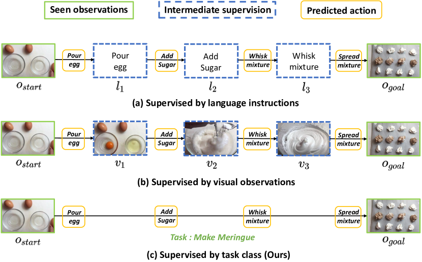
Figure 1: Procedure planning example. Given a start observation $o_{start}$ and a goal state $o_{goal}$, the model is required to generate a sequence of actions that can transform $o_{start}$ to $o_{goal}$. Previous approaches rely on heavy intermediate supervision during training, while our model only needs the task class labels (bottom row).

Previous approaches for procedure planning in instructional videos often treat it as a sequence planning problem and focus on predicting each action accurately. Most works rely on a two-branch autoregressive method to predict the intermediate states and actions step by step [34, 4, 2]. Such models are complex and easy to accumulate errors during the planning process, especially for long sequences. Recently, Zhao et al. [42] proposed a single branch non-autoregressive model based on transformer [38] to predict all intermediate steps in parallel. To obtain a good performance, they used a learnable memory bank in the transformer decoder, augmented their model with an extra generative adversarial framework [14] and applied a Viterbi post-processing method [39]. This method brought multiple learning objectives, complex training schemes and tedious inference process. Instead, we assume procedure planning as a distribution fitting problem and planning is solved with a sampling process. We aim to directly model the joint distribution of the whole action sequence in instructional video rather than every discrete action. In this perspective, we can use a simple MSE loss to optimize our generative model and generate action sequence plans in one shot with a sampling process, which results in less learning objectives and simpler training schemes.

For supervision in training, in addition to the action sequence, previous methods often require heavy intermediate visual [34, 4, 2] or language [42] annotations for their learning process. In contrast, we only use task labels from instructional videos as a condition for our learning (as shown in Fig. 1), which could be easily obtained from the keywords or captions of videos and requires much less labeling cost. Another reason is that task information is closely related to the action sequences in a video. For example, in a video of $jacking$ $up$ $a$ $car$, the possibility for action $add$ $sugar$ appears in this process is nearly zero.

Modeling the uncertainty in procedure planning is also an important factor that we need to consider. That is, there might be more than one reasonable plan sequences to transform from the given start state to goal state. For example, change the order of $add$ $sugar$ and $add$ $butter$ in $making$ $cake$ process will not affect the final result. So action sequences can vary even with the same start and goal states. To address this problem, we consider adding randomness to our distribution-fitting process and perform training with a diffusion model [19, 29]. Solving procedure planning problem with a diffusion model has two main benefits. First, a diffusion model changes the goal distribution to a random Gaussian noise by adding noise slowly to the initial data and learns the sampling process at inference time as an iterative denoising procedure starting from a random Gaussian noise. So randomness is involved both for training and sampling in a diffusion model, which is helpful to model the uncertain action sequences for procedure planning. Second, it is convenient to apply conditional diffusion process with the given start and goal observations based on diffusion models, so we can model the procedure planning problem as a conditional sampling process with a simple training scheme. In this work, we concatenate conditions and action sequences together and propose a projected diffusion model to perform conditional diffusion process.

Contributions. To sum up, the main contributions of this work are as follows: a) We cast the procedure planning as a conditional distribution-fitting problem and model the joint distribution of the whole intermediate action sequence as our learning objective, which can be learned with a simple training scheme. b) We introduce an efficient approach for training the procedure planner, which removes the supervision of visual or language features and relies on task supervision instead. c) We propose a novel projected diffusion model (PDPP) to learn the distribution of action sequences and produce all intermediate steps at one shot. We evaluate our PDPP on three instructional videos datasets and achieve the state-of-the-art performance across different prediction time horizons. Note that our model can still achieve excellent results even if we remove the task supervision and use the action labels only.

2 Related work

Procedural video understanding. The problem of procedural video understanding has gained more and more attention with an aim to learn the inter-relationship between different events in videos recently. Zhao et al. [43] investigated the problem of abductive visual reasoning, which requires vision systems to infer the most plausible visual explanation for the given visual observations. Furthermore, Liang et al. [26] proposed a new task: given an incomplete set of visual events, AI agents are asked to generate descriptions not only for the visible events and but also for the lost events by logical inferring. Unlike these works trying to learn the abductive information of intermediate events, Chang et al. [4] introduced procedure planning in instructional videos which requires AI systems to plan an action sequence that can transform the given start observation to the goal state. In this paper, we follow this work and study the procedural video understanding problem by learning goal-directed actions planning.

Diffusion probabilistic models. Nowadays, diffusion probabilistic models [31] have achieved great success in many research areas. Ho et al. [19] used a reweighted objective to train diffusion model and achieved great synthesis quality for image synthesis problem. Janner et al. [22] studied the trajectory planning problem with diffusion model and get remarkable results. Besides, diffusion models are also used in video generation[21, 18], density estimation[24], human motion[36], sound generation[41], text generation[25] and many other domains, all achieved competitive results. In this work, we apply diffusion process to procedure planning in instructional videos and propose our projected diffusion model, which achieves state-of-the-art performance only with a simple learning scheme.

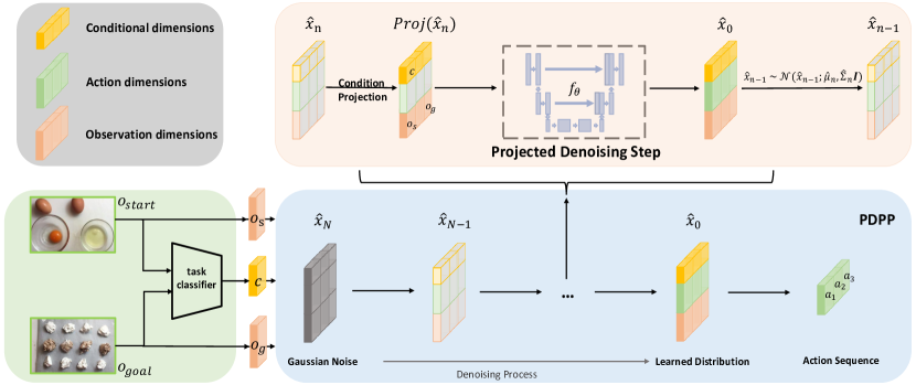
Figure 2: Overview of our projected diffusion model (prediction horizon $T$ = 3). We first train a task classifier to generate conditional information $c$, which will be used as guidance along with the given observations $o_{s}$ and $o_{g}$. Then we compute the denoising process iteratively. In each step, we first conduct a condition projection to the input, then predict the initial distribution by the learned model $f_{\theta}$. After that we calculate $\hat{x}_{n-1}$ with the predicted $\hat{x}_{0}$. We finally select the action dimensions as our result after $N$ denoising steps.

Projected gradient descent. Projected gradient descent is an optimal solution suitable for constrained optimization problems, which is proven to be effective in optimization with rank constraints [5], online power system optimization problems [15] and adversarial attack [6]. The core idea of projected gradient descent is to add a projection operation to the normal gradient descent method, so that the result is ensured to be constrained in the feasible region. Inspired by this, we add a similar projection operation to our diffusion process, which keeps the conditional information for diffusion unchangeable and thus provides accurate guides for learning.

3 Method

In this section, we present the details of our projected diffusion model for procedure planning (PDPP). We will first introduce the setup for this problem in Sec. 3.1. Then we present the diffusion model used to model the action sequence distribution in Sec. 3.2. To provide more precise conditional guidance both for the training and sampling process, a simple projection method is applied to our model, which we will discuss in Sec. 3.3. Finally, we show the training scheme (Sec. 3.4) and sampling process (Sec. 3.5) of our PDPP. An overview of PDPP is provided in Fig. 2.

3.1 Problem formulation

We follow the problem set-up of Chang et al. [4]: given a start visual observation $o_{s}$ and a visual goal $o_{g}$, a model is required to plan a sequence of actions $a_{1:T}$ so that the environment state can be transformed from $o_{s}$ to $o_{g}$. Here $T$ is the horizon of planning, which denotes the number of action steps for the model to take and {$o_{s}$, $o_{g}$} indicates two different environment states in an instructional video.

We decompose the procedure planning problem into two sub-problems, as shown in Eq. 1. The first problem is to learn the task-related information $c$ with the given {$o_{s}$, $o_{g}$} pair. This can be seen as a preliminary inference for procedure planning. Then the second problem is to generate action sequences with the task-related information and given observations. Note that Jing et al. [2] also decompose the procedure planning problem into two sub-problems, but their purpose of the first sub-problem is to provide long-horizon information for the second stage since Jing et al. [2] plans actions step by step, while our purpose is to get condition for sampling to achieve an easier learning.

$$p(a_{1:T}|o_{s},o_{g})=\int p(a_{1:T}|o_{s},o_{g},c)p(c|o_{s},o_{g})dc.$$ (1)

At training time, we first train a simple model (implemented as multi-layer perceptrons (MLPs)) with the given observations {$o_{s},o_{g}$} to predict which the task category is. We use the task labels in instructional videos $\overline{c}$ to supervise the output $c$. After that, we evaluate $p(a_{1:T}|o_{s},o_{g},c)$ in parallel with our model and leverage the ground truth (GT) intermediate action labels as supervision for training. Compared with the visual and language supervision in previous works, task label supervision is easier to get and brings simpler learning schemes. At inference phase, we just use the start and goal observations to predict the task class information $c$ and then samples action sequences $a_{1:T}$ from the learned distribution with the given observations and predicted $c$, where $T$ is the planning horizon.

3.2 Projected diffusion for procedure planning

Our method consists of two stages: task class prediction and action sequence distribution modeling. The first stage learning is a traditional classification problem which we implement with a simple MLP model. The main part of our model is the second one. That is, how to model $p(a_{1:T}|o_{s},o_{g},c)$ to solve the procedure planning problem. Jing et al. [2] assume this as a Goal-conditioned Markov Decision Process and use a policy $p(a_{t}|o_{t})$ along with a transition model $\tau_{\mu}(o_{t}|c,o_{t-1},a_{t-1})$ to perform the planning step by step, which is complex to train and slow for inference. We instead treat this as a direct distribution fitting problem with a diffusion model.

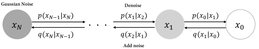
Figure 3: Schematic diagram for the forward and reverse diffusion processes.

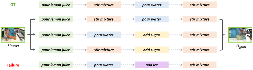
Figure 3: Visualization of diverse plans produced by our model with horizon $T=4$.

Diffusion model. A diffusion model [19, 29] solves the data generation problem by modeling the data distribution $p(x_{0})$ as a denoising Markov chain over variables {$x_{N}...x_{0}$} and assume $x_{N}$ to be a random Gaussian distribution. The forward process of a diffusion model is incrementally adding Gaussian noise to the initial data $x_{0}$ and can be represented as $q(x_{n}|x_{n-1})$, by which we can get all intermediate noisy latent variables $x_{1:N}$ with a diffusion step $N$. In the sampling stage, the diffusion model conducts iterative denoising procedure $p(x_{n-1}|x_{n})$ for $N$ times to approximate samples from the target data distribution. The forward and reverse diffusion processes are shown in Fig. 3.

In a standard diffusion model, the ratio of Gaussian noise added to the data at diffusion step $n$ is pre-defined as $\{\beta_{n}\in(0,1)\}_{n=1}^{N}$. Each adding noise step can be parametrized as

$$q(x_{n}|x_{n-1})=\mathcal{N}(x_{n};\sqrt{1-\beta_{n}}x_{n-1},\beta_{n}\textbf{I}).$$ (2)

Since hyper-parameters $\{\beta_{n}\}_{n=1}^{N}$ are pre-defined, there is no training in the noise-adding process. As discussed in [19], re-parameterize Eq. 2 we can get:

$$x_{n}=\sqrt{\overline{\alpha}_{n}}x_{0}+\sqrt{1-\overline{\alpha}_{n}}\epsilon,$$ (3)

where $\overline{\alpha}_{n}=\prod_{s=1}^{n}(1-\beta_{s})$ and $\epsilon\sim\mathcal{N}(0,I)$.

In the denoising process, each step is parametrized as:

$$p_{\theta}(x_{n-1}|x_{n})=\mathcal{N}(x_{n-1};\mu_{\theta}(x_{n},n),\Sigma_{\theta}(x_{n},n)),$$ (4)

where $\mu_{\theta}$ is produced by a learnable model and $\Sigma_{\theta}$ can be directly calculated with $\{\beta_{n}\}_{n=1}^{N}$ [19]. The learning objective for a typical diffusion model in [19] is the noise added to the uncorrupted data $x_{0}$ at each step. When training, the diffusion model first selects a diffusion step $n\in[1,N]$ and calculates $x_{n}$ as shown in Eq. 3. Then the learnable model will compute $\epsilon_{\theta}(x_{n},n)$ and calculate loss with the true noise add to the distribution at step $n$. After training, the diffusion model can simply generate data like $x_{0}$ by iteratively processing the denoising step starting from a random Gaussian noise.

However, applying this kind of diffusion model to procedure planning directly is not suitable. First, the sampling process in our task is condition-guided while no condition is applied in the standard diffusion model. Second, the distribution we want to fit is the whole action sequence, which has a strong semantic information. Directly predicting the semantically meaningless noise sampled from random Gaussian distribution can be hard. In experiments which take noise as the predicting objective, our model just fails to be trained. To address these problems, we make two modifications to the standard diffusion model: one is about input and the other is the learning objective of model.

Conditional action sequence input. The input of a standard diffusion model is the data distribution it needs to fit and no guided information is required. For the procedure planning problem, the distribution we aim to fit is the intermediate action sequences $[a_{1},a_{2}...a_{T}]$, which depends on the given observations and task class we get in the first learning stage. Thus we need to find how to add these guided conditions into the diffusion process. Although there are multiple guided diffusion models presented [7, 20], they are expensive for learning and need complex training or sampling strategy. Inspired by Janner et al. [22], we here apply a simple way to achieve our goal: just treat these conditions as additional information and concatenate them along the action feature dimension. Notably, we concatenate $o_{s}$ and $a_{1}$ together, same for $o_{g}$ and $a_{T}$. In this way, we introduce a prior knowledge that the start/end observations are more related to the first/last actions, which turns out to be useful for our learning (details are provided in the supplementary material). Thus our model input for training now can be represented as a multi-dimension array:

$$\begin{bmatrix}c&c&&c&c\\ a_{1}&a_{2}&...&a_{T-1}&a_{T}\\ o_{s}&0&&0&o_{g}\end{bmatrix}.$$ (5)

Each column in our model input represents the condition information, action one-hot code, and the corresponding observation for a certain action. Note that we do not need the intermediate visual observations as supervision, so all observation dimensions are set to zero except for the start and end observations.

Learning objective of our diffusion model. As mentioned above, the learning objective of a standard diffusion model is the random noise added to the distribution at each diffusion step. This learning scheme has demonstrated great success in data synthesis area, partly because predicting noise rather than the initial input $x_{0}$ brings more variations for data generation. For procedure planning problem, however, the distribution we need to fit contains high-level features rather than pixels. Since the planning horizon $T$ is relatively short and the one-hot action features require less randomness than in data generation, predicting noise in diffusion process for procedure planning will just increase the difficulty of learning. So we modify the learning objective to the initial input $x_{0}$, which will be described in Sec. 3.4.

3.3 Condition projection during learning

Our model transforms a random Gaussian noise to the final result, which has the same structure with our model input (see Eq. 5) by conducting $N$ denoising steps. Since we combine the conditional information with action sequences as the data distribution, these conditional guides can be changed during the denoising process. However, the change of these conditions will bring wrong guidance for the learning process and make the observations and conditions useless. To address this problem, we add a condition projection operation into the learning process. That is, we force the observation and condition dimensions not to be changed during training and inference by assigning the initial value. The input $x$ of condition projection is either a noise-add data (Alg.1 L5) or the predicted result of model (Alg.1 L7). We use $\{\hat{c},\hat{a},\hat{o}\}$ to represent different dimensions in $x$, then our projection operation $\mathrm{Proj}()$ can be denoted as:

$$\begin{bmatrix}\hat{c}_{1}&\hat{c}_{2}&&&\hat{c}_{T}\\ \hat{a}_{1}&\hat{a}_{2}&...&&\hat{a}_{T}\\ \hat{o}_{1}&\hat{o}_{2}&&&\hat{o}_{T}\end{bmatrix}\to\begin{bmatrix}c&c&&&c\\ \hat{a}_{1}&\hat{a}_{2}&...&&\hat{a}_{T}\\ o_{s}&0&&&o_{g}\end{bmatrix},$$ (6)

$$x\qquad\qquad\qquad\qquad\mathrm{Proj}(x)$$

where $\hat{c}_{i}$, $\hat{o}_{i}$ and $\hat{a}_{i}$ denote the $i^{th}$ horizon class, observation dimensions and predicted action logits in $x$, respectively. $c$, $o_{s},o_{g}$ are the conditions.

3.4 Training scheme

Our training scheme contains two stages: a) training a task-classifier model $\mathcal{T}_{\phi}(c|o_{s},o_{g})$ that extracts conditional guidance from the given start and goal observations; b) leveraging the projected diffusion model to fit the target action sequence distribution.

For the first stage, we apply MLP models to predict the task class $c$ with the given $o_{s},o_{g}$. Ground truth task class labels $\overline{c}$ are used as supervision. In the second learning stage, we follow the basic training scheme for diffusion model, but change the learning objective as the initial input $x_{0}$. We use a U-Net model [30] $f_{\theta}(x_{n},n)$ as the learnable model and our training loss is:

$$\mathcal{L}_{\mathrm{diff}}=\sum_{n=1}^{N}(f_{\theta}(x_{n},n)-x_{0})^{2},$$ (7)

We believe that $a_{1}$ and $a_{T}$ are more important because they are the most related actions for the given observations. Thus we rewrite Eq. 7 as a weighted loss by multiplying a weight matrix to $\mathcal{L}_{\mathrm{diff}}$ as follows:

$$\begin{bmatrix}1&1&&1&1\\ w&1&...&1&w\\ 1&1&&1&1\end{bmatrix}.$$ (8)

Besides, we add a condition projection step to our diffusion process. So given the initial input $x_{0}$ which contains action sequences, task conditions and observations, we first add noise to the input to get $x_{n}$, and then apply condition projection to ensure the guidance not changed. With $x_{n}$ and the corresponding diffusion step $n$, we calculate the denosing output $f_{\theta}(x_{n},n)$, followed by condition projection again. Finally, we compute the weighted $\mathcal{L}_{\mathrm{diff}}$ and update model, as shown in Algorithm 1.

Algorithm 1 Training

1:Initial input $x_{0}$, total diffusion steps number $N$, model $f_{\theta}$, $\{\overline{\alpha}_{n}\}_{n=1}^{N}$, weight matrix $w$

2:repeat

3:     $n\sim Uniform(\{1,...,N\})$

4:     $\epsilon\sim\mathcal{N}(0,I)$

5:     $x_{n}=\sqrt{\overline{\alpha}_{n}}x_{0}+\sqrt{1-\overline{\alpha}_{n}}\epsilon$

6:     $\hat{x}_{0}=f_{\theta}(Proj(x_{n}),n)$

7:     Take gradient descent step on

8:      $\bigtriangledown_{\theta}\left|\left|\left(x_{0}-Proj(\hat{x}_{0})\right)*w\right|\right|^{2}$

9:until converged

3.5 Inference

At inference time, only the start observation $o_{s}$ and goal observation $o_{g}$ are provided. We first predict the task class by choosing the maximum probability value in the output of task-classifier model $\mathcal{T}_{\phi}$. Then the predicted task class $c$ is used as the class condition. To sample from the learned action sequence distribution, we start with a Gaussian noise, and iteratively conduct denoise and condition projection for $N$ times. The detailed inference process is shown in Algorithm 2.

Algorithm 2 Inference

1:total diffusion steps number $N$, model $f_{\theta}$, $\{\overline{\alpha}_{n}\}_{n=1}^{N}$, $\{\beta_{n}\}_{n=1}^{N}$

2:$\hat{x}_{N}\sim\mathcal{N}(0,I)$

3:for $n=N,...,1$ do

4:     $\hat{x}_{0}=f_{\theta}(Proj(\hat{x}_{n}),n)$

5:     if $n>1$ then

6:         $\hat{\mu}_{n}=\frac{\sqrt{\overline{\alpha}_{n-1}}\beta_{n}}{1-\overline{\alpha}_{n}}\hat{x}_{0}+\frac{\sqrt{\alpha_{n}}(1-\overline{\alpha}_{n-1})}{1-\overline{\alpha}_{n}}\hat{x}_{n}$

7:         $\hat{\Sigma}_{n}=\frac{1-\overline{\alpha}_{n-1}}{1-\overline{\alpha}_{n}}\cdot\beta_{n}$

8:         $\hat{x}_{n-1}\sim\mathcal{N}(\hat{x}_{n-1};\hat{\mu}_{n},\hat{\Sigma}_{n}\textbf{I})$

9:     end if

10:end for

11:return $\hat{x}_{0}$

Once we get the predicted output $\hat{x}_{0}$, we take out the action sequence dimensions $[\hat{a}_{1},...,\hat{a}_{T}]$ and select the index of every maximum value in $\hat{a}_{i}(i=1,...,T)$ as the action sequence plan for procedure planning. Note that for the training stage, the class condition dimensions of $x_{0}$ are the ground truth task labels, not the output of our task-classifier as in inference.

4 Experiments

In this section, we evaluate our PDPP model on three real-life datasets and show our competitive results for various planning horizons. We first present the result of our first training stage, which predicts the task class with the given observations in Sec. 4.3. Then we compare our performance with other alternative approaches on the three datasets and demonstrate the effectiveness of our model in Sec. 4.4. We also study the role of task-supervision for our model in Sec. 4.5. Finally, we show our prediction uncertainty evaluation results in Sec. 4.6.

4.1 Implementation details

We use the basic U-Net [30] as our learnable model for projection diffusion, in which a modification is made by using a convolution operation along the planning horizon dimension for downsampling rather than max-pooling as in [22]. For training, we use the linear warm-up training scheme to optimize our model. We train different steps for the three datasets, corresponding to their scales. More details about training and model architecture are provided in the supplementary material.

4.2 Evaluation protocol

Datasets. We evaluate our PDPP model on three instructional video datasets: CrossTask [44], NIV [1], and COIN [35]. CrossTask contains 2,750 videos from 18 different tasks, with an average of 7.6 actions per video. The NIV dataset consists of 150 videos about 5 daily tasks, which has 9.5 actions in one video on average. COIN is much larger with 11,827 videos, 180 different tasks and 3.6 actions/video. We randomly select 70% data for training and 30% for testing as previous work [4, 2, 42]. Note that we do not select 70%/30% for videos in each task, but in the whole dataset. Following previous work[4, 2, 42], we extract all action sequences $\{[a_{i},...,a_{i+T-1}]\}_{i=1}^{n-T+1}$ with predicting horizon $T$ from the given video which contains $n$ actions by sliding a window of size $T$. Then for each action sequence $[a_{i},...,a_{i+T-1}]$, we choose the video clip feature at the beginning time of action $a_{i}$ and clip feature around the end time of $a_{i+T-1}$ as the start observation $o_{s}$ and goal state $o_{g}$, respectively. Both clips are 3 seconds long. For experiments conduct on CrossTask, we use two kinds of pre-extracted video features as the start and goal observations. One are the features provided in CrossTask dataset: each second of video content is encoded into a 3200-dimensional feature vector as a concatenation of the I3D, ResNet-152 and audio VGG features[16, 17, 3], which are also applied in [2, 4]. The other kind of features are generated by the encoder trained with the HowTo100M[27] dataset, as in [42]. For experiments on the other two datasets, we follow [42] to use the HowTo100M features for a fair comparison.

	CrossTaskBase	CrossTaskHow	COIN	NIV
$T$ = 3	83.87	92.43	79.42	100.00
$T$ = 4	83.64	92.98	78.89	100.00
$T$ = 5	83.37	93.39	-	-
$T$ = 6	83.85	93.20	-	-

Table 1: Classification results on all datasets. CrossTask_Base uses features provided by the dataset while CrossTask_How applies features extracted by HowTo100M trained encoder.

		$T$ = 3			$T$ = 4
Models	Supervision	SR$\uparrow$	mAcc$\uparrow$	mIoU$\uparrow$	SR$\uparrow$	mAcc$\uparrow$	mIoU$\uparrow$
Random	-	$<$0.01	0.94	1.66	$<$0.01	0.83	1.66
Retrieval-Based	-	8.05	23.30	32.06	3.95	22.22	36.97
WLTDO[10]	-	1.87	21.64	31.70	0.77	17.92	26.43
UAAA[11]	-	2.15	20.21	30.87	0.98	19.86	27.09
UPN[33]	V	2.89	24.39	31.56	1.19	21.59	27.85
DDN[4]	V	12.18	31.29	47.48	5.97	27.10	48.46
Ext-GAILw/o Aug.[2]	V	18.01	43.86	57.16	-	-	-
Ext-GAIL[2]	V	21.27	49.46	61.70	16.41	43.05	60.93
P3IV[42]	L	23.34	49.96	73.89	13.40	44.16	70.01
OursBase	C	25.52	53.43	56.90	15.40	49.42	56.99
OursHow	C	37.20	64.67	66.57	21.48	57.82	65.13

Table 2: Evaluation results on CrossTask for procudure planning with prediction horizon $T\in\{3,4\}$. The $Supervision$ column denotes the type of supervision applied in training, where V denotes intermediate visual states, L denotes language feature and C means task class. Note that we compute mIoU by calculating average of every IoU of a single antion sequence rather than a mini-batch.

Metrics. Following previous work[4, 2, 42], we apply three metrics to evaluate the performance. a) Success Rate (SR) considers a plan as a success only if every action matches the ground truth sequence. b) mean Accuracy (mAcc) calculates the average correctness of actions at each individual time step, which means an predicted action is considered correct if it matches the action in ground truth at the same time step. c) mean Intersection over Union (mIoU) measures the overlap between predicted actions and ground truth by computing Iou $\frac{|\{a_{t}\}\cap\{\hat{a_{t}}\}|}{|\{a_{t}\}\cup\{\hat{a_{t}}\}|}$, where $\{a_{t}\}$ is the set of ground truth actions and $\{\hat{a_{t}}\}$ is the set of predicted actions.

Previous approaches [42, 2] compute the mIoU metric on every mini-batch (batch size larger than one) and calculate the average as the result. This brings a problem that the mIoU value can be influenced heavily by batch size. Consider if we set batch size is equal to the size of training data, then all predicted actions can be involved in the ground truth set and thus be correct predictions. However, if batch size is set to one, then any predicted action that not appears in the corresponding ground truth action sequence will be wrong. To address this problem, we standardize the way to get mIoU as computing IoU on every single sequence and calculating the average of these IoUs as the result (equal to setting of batch size $=1$).

Baselines. Models for procedure planning[4, 2, 42] and other fully supervised planning approaches[11, 10, 33] are all involved in our comparison. Descriptions for these methods are available in the supplementary material.

	$T$ = 3	$T$ = 4	$T$ = 5	$T$ = 6
Models	SR$\uparrow$	SR$\uparrow$	SR$\uparrow$	SR$\uparrow$
Retrieval-Based	8.05	3.95	2.40	1.10
DDN[4]	12.18	5.97	3.10	1.20
P3IV[42]	23.34	13.40	7.21	4.40
OursBase	25.52	15.40	9.37	6.76
OursHow	37.20	21.48	13.45	8.41

Table 3: Success Rate evaluation results on CrossTask with longer planning horizons.

4.3 Results for task-classifier

The first stage of our learning is to predict the task class with the given start and goal observations. We implement this with MLP models and the detailed first-stage training process is described in the supplementary material. The classification results for different planning horizons on three datasets are shown in Tab. 1. We can see that our classifier can perfectly figure out the task class in the NIV dataset since only 5 tasks are involved. For larger datasets CrossTask and COIN, our model can make right predictions most of the time.

4.4 Comparison with other approaches

We follow previous work[42] and compare our approach with other alternative methods on three datasets, across multiple prediction horizons.

			NIV			COIN
Horizon	Models	Sup.	SR$\uparrow$	mAcc$\uparrow$	mIoU$\uparrow$	SR$\uparrow$	mAcc$\uparrow$	mIoU$\uparrow$
$T$ = 3	Random	-	2.21	4.07	6.09	$<$0.01	$<$0.01	2.47
	Retrieval	-	-	-	-	4.38	17.40	32.06
	DDN [4]	V	18.41	32.54	56.56	13.9	20.19	64.78
	Ext-GAIL [2]	V	22.11	42.20	65.93	-	-	-
	P3IV [42]	L	24.68	49.01	74.29	15.4	21.67	76.31
	Ours	C	30.20	48.45	57.28	21.33	45.62	51.82
$T$ = 4	Random	-	1.12	2.73	5.84	$<$0.01	$<$0.01	2.32
	Retrieval	-	-	-	-	2.71	14.29	36.97
	DDN [4]	V	15.97	27.09	53.84	11.13	17.71	68.06
	Ext-GAIL [2]	V	19.91	36.31	53.84	-	-	-
	P3IV [42]	L	20.14	38.36	67.29	11.32	18.85	70.53
	Ours	C	26.67	46.89	59.45	14.41	44.10	51.39

Table 4: Evaluation results on NIV and COIN with prediction horizon $T\in\{3,4\}$. Sup. denotes the type of supervision in training. Note that we compute IoU on every action sequence and take the mean as mIoU.

CrossTask (short horizon). We first evaluate on CrossTask with two prediction horizons typically used in previous work. We use Ours_Base to denote our model with features provided by CrossTask and Ours_How as model with features extracted by HowTo100M trained encoder. Note that we compute mIoU by calculating the mean of every IoU for a single antion sequence rather than a mini-batch as explained in Sec. 4.2, though the latter can achieve a higher mIoU value. Results in Tab. 2 show that Ours_Base beats all methods for most metrics except for the success rate (SR) when $T=4$, where our model is the second best, and Ours_How just significantly outperforms all previous methods. Specifically, for using HowTo100M-extracted video features, we outperform [42] by around 14% and more than 8% for SR when $T=3,4$, respectively. As for features provided by CrossTask, Ours_Base outperforms the previous best method [2] by around 4% both for SR and mAcc when $T=3$.

CrossTask (long horizon). We further study the ability of predicting with longer horizons for our model. Following [42], we here evaluate the SR value with planning horizon $T=\{3,4,5,6\}$. We present the result of our model along with other approaches that reported results for longer horizons in Tab. 3. This result shows our model can get a stable and great improvement with all planning horizons compared with the previous best model.

NIV and COIN. Tab. 4 shows our evaluation results on the other two datasets NIV and COIN, from which we can see that our approach remains to be the best performer for both datasets. Specifically, in the NIV dataset where mAcc is relatively high, our model raises the SR value by more than 6% both for the two horizons and outperforms the previous best by more than 8% on mAcc metric when $T=4$. As for the large COIN dataset where mAcc is low, our model significantly improves mAcc by more than 20%.

All the results suggest that our model performs well across datasets with different scales.

4.5 Study on task supervision

In this section, we study the role of task supervision for our model. Tab. 5 shows the results of learning with and without task supervision, which suggest that the task supervision is quite helpful to our learning. Besides, we find that task supervision helps more for learning in the COIN dataset. We assume the reason is that fitting the COIN dataset is hard to our model since the number of tasks in COIN is large. Thus the guidance of task class information is more important to COIN compared with the other two datasets. Notably, training our model without task supervision also achieves state-of-the-art performance on multiple metrics, which suggests the effective of our approach.

	Dataset	w. task sup.			w.o. task sup.
		SR$\uparrow$	mAcc$\uparrow$	mIoU$\uparrow$	SR$\uparrow$	mAcc$\uparrow$	mIoU$\uparrow$
$T$ = 3	CrossTaskBase	25.52	53.43	56.90	22.82	51.56	54.36
	CrossTaskHow	37.20	64.67	66.57	35.69	63.91	66.04
	NIV	30.20	48.45	57.28	28.37	45.96	54.31
	COIN	21.33	45.62	51.82	16.48	36.57	43.48
$T$ = 4	CrossTaskBase	15.40	49.42	56.99	14.91	49.55	56.28
	CrossTaskHow	21.48	57.82	65.13	20.52	57.47	64.39
	NIV	26.67	46.89	59.45	26.50	46.08	58.94
	COIN	14.41	44.10	51.39	11.65	35.04	41.75
$T$ = 5	CrossTaskBase	9.37	45.93	56.32	8.95	45.77	56.34
	CrossTaskHow	13.45	54.01	65.32	12.80	53.44	64.01
$T$ = 6	CrossTaskBase	6.76	43.61	57.51	6.06	44.15	57.07
	CrossTaskHow	8.41	49.65	64.70	8.15	50.45	64.13

Table 5: Ablation study on the role of task supervision. The $w.$ $task$ $sup.$ denotes learning with task supervision and $w.o.$ $task$ $sup.$ means training with the basic action labels only.

4.6 Evaluating probabilistic modeling

As discussed in Sec. 1, we introduce diffusion model to procedure planning to model the uncertainty in this problem. Here we follow [42] to evaluate our probabilistic modeling. We focus on CrossTask_How as it has the most uncertainty for planning. Results on other datasets and further details are available in the supplement.

Our model is probabilistic by starting from random noises and denoising step by step. We here introduce two baselines to compare with our diffusion based approach. We first remove the diffusion process in our method to establish the Noise baseline, which just samples from a random noise with the given observations and task class condition in one shot. Then we further establish the Deterministic baseline by setting the start distribution $\hat{x}_{N}=0$, thus the model directly predicts a certain result with the given conditions. We reproduce the KL divergence, NLL, ModeRec and ModePrec in [42] and use these metrics along with SR to evaluate our probabilistic model. The results in Tab. 6 and Tab. 7 suggest our approach has an excellent ability to model the uncertainty in procedure planning and can produce both diverse and reasonable plans(visualizations available in the supplement). Specifically, our approach improves ModeRec greatly for longer horizons. There is less uncertainty when $T$ = 3, thus the diffusion based models performs worse than the deterministic one.

Metric$\downarrow$	Model	T = 3	T=4	T=5	T=6
NLL	Deterministic	3.57	4.29	4.70	5.12
	Noise	3.58	4.04	4.45	4.79
	Ours	3.61	3.85	3.77	4.06
KL-Div	Deterministic	2.99	3.40	3.54	3.82
	Noise	3.00	3.15	3.30	3.49
	Ours	3.03	2.96	2.62	2.76

Table 6: Evaluation results of the plan distributions metrics.

Metric$\uparrow$	Model	T = 3	T=4	T=5	T=6
SR	Deterministic	38.79	21.17	12.59	7.47
	Noise	34.92	18.99	12.04	7.82
	Ours	37.20	21.48	13.45	8.41
ModePrec	Deterministic	55.60	45.65	35.47	25.24
	Noise	51.04	43.90	34.35	24.51
	Ours	53.14	44.55	36.30	25.61
ModeRec	Deterministic	34.13	18.35	11.20	6.75
	Noise	39.42	25.56	15.67	11.04
	Ours	36.49	31.10	29.45	22.68

Table 7: Evaluation results of diversity and accuracy metrics.

5 Conclusion

In this paper, we have casted procedure planning in instructional videos as a distribution fitting problem and addressed it with a projected diffusion model. Compared with previous work, our model requires less supervision and can be trained with a simple learning objective. We evaluate our approach on three datasets with different scales and find our model achieves the state-of-the-art performance among multiple planning horizons. Our work demonstrates that modeling action sequence as a whole distribution is an effective solution to procedure planning in instructional videos, even without intermediate supervision.

Acknowledgements. This work is supported by the National Key R$\&$D Program of China (No. 2022ZD0160900), the National Natural Science Foundation of China (No. 62076119, No. 61921006), the Fundamental Research Funds for the Central Universities (No. 020214380091), and the Collaborative Innovation Center of Novel Software Technology and Industrialization.

A Supplementary Material

Our supplementary material consists of the following: Sec. B provides the details of our model architecture, training process and dataset curation. Sec. C describes the baselines we compare with. Sec. D shows the details of training the task classifier in the first learning stage. We talk about another different evaluation protocol used by previous approach[34] and present the performance of our model with this protocol in Sec. E. Then in Sec. F, we study how batch size affects the value of mIoU metric and show the results of evaluating mIoU with different batch size on the same model. In Sec. G, we discuss the importance of introducing prior knowledge that the start/end observations are more related to the first/last actions to our model. Finally, we provide more results, details and visualizations about the ability to model uncertainty of our approach in Sec. H.

B Implementation Details

B.1 Details of model architecture

The maintain of our model is the learnable model $f_{\theta}$, which we implement as a basic 3-layer U-Net[30]. As in [22], each layer in our model consists of two residual blocks[16] and one downsample or upsample operation. One residual block consists of two convolutions, each followed by a group norm[40] and Mish activation function[28]. Time embedding is produced by a fully-connected layer and added to the output of first convolution. We apply a 1d-convolution along the planning horizon dimension as the downsample/upsample operation. Considering that the value of planning horizon is small ($T=\{3,4,5,6\}$), we set the kernel size of 1d-convolution as $2$, stride as $1$, padding as $0$ so the length change of planning horizon dimension keeps $1$ after each downsample or upsample.

The input for our model is the concatenation of task class, actions labels and observation features, so the size of feature dimension is $dim=L_{c}+L_{a}+L_{o}$. Here $L_{c}$ means the number of task classes in the dataset, $L_{a}$ is the number of different actions in the dataset and $L_{o}$ is the length of visual features. Our model embeds the input feature with shape $[dim\to 256\to 512\to 1024]$ in the downsample process and recover to the initial size in the upsample process as $[1024\to 512\to 256\to dim]$.

For diffusion, we use the cosine noise schedule to produce the hyper-parameters $\{\beta_{n}\}_{n=1}^{N}$, which denote the ratio of Gaussian noise added to the data at each diffusion step.

B.2 Dataset curation details

Each video in the dataset is annotated with action labels and temporal boundaries. That is, the start time and end time of each action in an instructional video are annotated as $\{s_{i},e_{i}\}_{i=1}^{num}$, where $s_{i}$ and $e_{i}$ denote the start and end time of the $i_{th}$ action, $num$ denotes the number of actions in the video. We in this paper follow previous work[4, 2] to extract all action sequences with predicting horizon $T$ $\{[a_{i},...,a_{i+T-1}]\}_{i=1}^{num-T+1}$ from the given video which contains $num$ actions by sliding a window of size $T$. Thus each action sequence we need to predict can be presented as $\{a_{i},a_{i+1},...,a_{i+T-1}\}$. We choose the video clip feature at the beginning time of action $a_{i}$ and clip feature around the end time of $a_{i+T-1}$ as the start observation $o_{s}$ and goal state $o_{g}$, respectively. Specifically, we first round the start and end time of this action sequence to get $\left\lfloor s_{i}\right\rfloor$ and $\left\lceil e_{i+T-1}\right\rceil$. Then we choose clip feature starts from $\left\lfloor s_{i}\right\rfloor$ and clip feature ends with $\left\lceil e_{i+T-1}\right\rceil$ as $o_{s},o_{g}$, as shown in Fig. 1. Both clips are 3 seconds long.

B.3 Details of training process

We train our model with a linear warm-up scheme. For different datasets, the training scheme changes due to different scales. In CrossTask_Base, we set the diffusion step as $200$ and train our model for $12,000$ steps with learning rate increasing linearly to $8\times 10^{-4}$ in the first $4,000$ steps. Then the learning rate decays to $4\times 10^{-4}$ at step $10,000$. In CrossTask_How, we keep diffusion step as 200 and train our model for $24,000$ steps with learning rate increasing linearly to $5\times 10^{-4}$ in the first $4,000$ steps and decays by 0.5 at step $10,000,16,000$ and $22,000$. In NIV, the diffusion step is $50$ and we train $6,500$ steps due to its small size. The learning rate increases linearly to $3\times 10^{-4}$ in the first $4,500$ steps and decays by $0.5$ at step $6,000$. The COIN dataset requires much more training steps due to its large scale. We set diffusion step as $200$ and train our model for $160,000$ steps. The learning rate increases linearly to $1\times 10^{-5}$ in the first $4,000$ steps and decays by $0.5$ at step $14,000$ and step $24,000$. Then we keep learning rate as $2.5\times 10^{-6}$ for the remaining training steps. The training batch size for all experiments is $256$. For the weighted loss in our training process, we set $w=10$. All our experiments are conducted with ADAM[23] on 8 NVIDIA TITAN Xp GPUs.

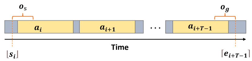
Figure 1: Selection of observations with a given action sequence.

C Baselines

Choices	T = 3	T=4	T=5	T=6
MLP+Crossentropy	81.94	82.61	83.14	84.08
ResMLP+Crossentropy	81.60	82.47	82.77	82.83
ResMLP+MSEloss	83.87	83.64	83.37	83.85

Table 1: Task classification results in the first stage with different training choices for CrossTask_Base.

In this section, we introduce the baselines we used in our paper.

- $Random$. This policy randomly selects actions from the available action space in dataset to produce the plans.

- $Retrieval$-$Based$. Given the observations $\{o_{s},o_{g}\}$, the retrieval-based method retrieves the closest neighbor by calculating the minimum visual feature distance in the train dataset. Then the action sequence associated with the retrieved result will be used as the action plan.

- $WLTDO$[10]. This approach applies a recurrent neural network(RNN) to predict action steps with the given observation pairs.

- $UAAA$[11]. UAAA is a two-stage approach which uses RNN-HMM model to predict action steps autoregressively.

- $UPN$[33]. UPN is a physical-world path planning algorithm and learns a plannable representation to make predictions. To produce the discrete action steps, we follow [4] to add a softmax layer to the output of this model.

- $DDN$[4]. DDN model is a two-branch autoregressive model, which learns an abstract representation of action steps and tries to predict the state-action transition in the feature space.

- $PlaTe$[34]. PlaTe model follows DDN and uses transformer modules in two-branch to predict instead. Note that the evaluation protocol of PlaTe is different with other models, so we move the comparison with PlaTe to supplementary material, which we will discuss later.

- $Ext$-$GAIL$[2]. This model solves the procedure planning problem by reinforcement learning techniques. Similar to our work, Ext-GAIL decomposes the procedure planning problem into two sub-problems. However, the purpose of the first sub-problem in Ext-GAIL is to provide long-horizon information for the second stage while our purpose is to get condition for sampling.

- $P^{3}IV$[42]. P³IV is a single-branch transformer-based model which augments itself with a learnable memory bank and an extra generative adversarial framework. Like our model, P³IV predicts all action steps at once during inference process.

D Details of the first learning stage

In the first learning stage, we need to predict the task class with the given observations $\{o_{s},o_{g}\}$. We use a simple 4-layer MLP model to achieve this and calculate the cross entropy loss for the output of the model and the ground truth task class label to train our model, except for CrossTask_Base. A two-layer Res-MLP [37] trained with MSE loss is applied to CrossTask_Base. The task classification results in the first learning stage for different models with different training losses on CrossTask_Base are shown in Tab. 1.

E Evaluation with another evaluation protocol

As talked in Sec. C, PlaTe[34] used another protocol for evaluation. P³IV[42] later evaluated SR with this protocol to compare with PlaTe. We name this as ”protocol 2”. In all experiments of the main paper, we follow previous work[4, 2, 42] to use a 70%/30% split for training/testing and rely on a sliding window to get our learning data. In this section, we evaluate our model with ”protocol 2” and compare our performance with previous works that evaluated with this protocol.

The main differences of ”protocol 2” are as followed: a) ”protocol 2” uses a 2390/360 split for train/test. b) ”protocol 2” randomly selects one procedure plan with prediction horizon $T$ in each video for training and testing, rather than relying on a $T$-$size$ sliding window to consider all procedure plans in each video. c) Given the planning horizon $T$, ”protocol 2” only predicts $T-1$ actions.

We evaluate our model with ”protocol 2” on CrossTask and compare the results with the previous best approach, considering both short and long horizons. Specifically, we use CrossTask_Base to compare with PlaTe for shorter horizons and CrossTask_How to compare with P³IV for longer horizons. In this way we align the visual features used in different approaches with our model to conduct a fair comparison. The task classification accuracy results for $T$ = $\{3,4,5,6\}$ with ”protocol 2” are provided in Tab. 2. Tab. 3 shows the results of our model with short horizons, and Tab. 4 shows the results of SR metric with longer prediction horizons. Note that we compute mIoU by calculating the mean of every IoU for a single antion sequence rather than a mini-batch. We can see that our method keeps the top performance for all prediction horizons.

Model	T = 3	T=4	T=5	T=6
CrossTaskBase	81.71	83.63	84.65	84.53
CrossTaskHow	91.78	93.31	93.50	93.75

Table 2: Task classification results with protocol2.

Models	T = 3			T = 4
	SR$\uparrow$	mAcc$\uparrow$	mIoU$\uparrow$	SR$\uparrow$	mAcc$\uparrow$	mIoU$\uparrow$
PlaTe[34]	16.00	36.17	65.91	14.00	35.29	55.36
OursBase	33.61	50.83	49.86	24.17	51.48	54.33

Table 3: Evaluation results with protocol2 on CrossTask. Prediction horizon set to $T=\{3,4\}.$ Note that we compute IoU on every action sequence and take the mean as mIoU.

Models	T = 3	T = 4	T = 5	T = 6
	SR$\uparrow$	SR$\uparrow$	SR$\uparrow$	SR$\uparrow$
P3IV[42]	24.4	15.8	11.8	8.3
OursHow	53.06	35.28	21.39	13.33

Table 4: Evaluation results of SR with protocol 2 on CrossTask. Prediction horizon set to $T=\{3,4,5,6\}.$

F Impact of batch size on mIoU

As we discussed in the main paper, previous approaches calculate the IoU value on every mini-batch and take their mean as the final mIoU. However, the batch size value for different methods may be different, which results in an unfair comparison. In this section, we study the impact of batch size on mIoU, which can illustrate the importance for the standardization of computing mIoU.

We use our trained models to compute the mIoU metric on CrossTask with different evaluation batch size. Planning horizon is set to $\{3,4,5,6\}$. The results are shown in Tab. 5, which validate our thought and show the huge impact of batch size on mIoU. The value of mIoU evaluated on the same model can vary widely as batch size changes, so comparing mIoU with different evaluation batch size has no meaning. To address this problem, we standardize the way to compute mIoU as setting evaluation batch size to 1 at inference time.

	Batch size	T = 3	T=4	T=5	T=6
OursBase	1	56.90	56.99	56.32	57.51
	4	65.30	67.14	67.10	70.48
	8	68.83	69.64	67.39	69.31
	16	69.79	67.26	64.53	63.19
OursHow	1	66.57	65.13	65.32	65.38
	4	75.21	77.07	78.56	78.59
	8	79.74	81.74	81.73	80.88
	16	80.50	82.32	81.41	78.64

Table 5: Evaluation results of mIoU with different batch size on CrossTask.

G Role of prior knowledge

In this section, we study the role of leveraging a prior knowledge that the start/end observations are more related to the first/last actions for our model.

Inspired by [13], we establish a baseline not using this prior knowledge by tiling the observations and task class conditions to the output of the U-Net encoder before decoding. A residual convolution block is applied to reduce the channel dimension of observation features. Then the features and conditions are replicate $k$ times($k$ is the horizon length of the U-Net encoder output) and concatenated along the channel dimension. We conduct experiments on CrossTask and the results are shown in Tab. 6, which demonstrates that the introduced prior knowledge is quite useful to the learning process with visual features provided by CrossTask(Ours_Base), while not good when better visual features are provided(Ours_How).

	T=3			T=4
	SR$\uparrow$	mAcc$\uparrow$	mIoU$\uparrow$	SR$\uparrow$	mAcc$\uparrow$	mIoU$\uparrow$
TileBase	22.34	49.10	53.71	14.13	45.80	55.03
OursBase	25.52	53.43	56.90	15.40	49.42	56.99
TileHow	36.21	65.12	66.79	22.31	59.00	66.20
OursHow	37.20	64.67	66.57	21.48	57.82	65.13

Table 6: Ablation study on the role of prior knowledge.

H Additional study on modeling uncertainty

In the main paper, we study the probabilistic modeling ability of our model on CrossTask_How and show that our diffusion based model can produce both diverse and accurate plans. Here we provide more details, results and visualizations about modeling the uncertainty in procedure planning by our model.

Details of evaluating uncertainty modeling. For the Deterministic baseline, we just sample once to get the plan since the result for Deterministic is certain when observations and task class conditions are given. For the Noise baseline and our diffusion based model, we sample 1500 action sequences as our probabilistic result to calculate the uncertain metrics. Furthermore, in order to efficiently complete the process of 1500 sampling, we apply the DDIM [32] sampling method to our model, with which one sampling process can be completed with 10 steps(accelerating the sampling for CrossTask and COIN by 20 times and NIV by 5 times). Note that the multiple sampling process is only required while evaluating probabilistic modeling and our model can generate a good plan just by sampling once.

	T=3		T=4
	KL-Div$\downarrow$	NLL$\downarrow$	KL-Div$\downarrow$	NLL$\downarrow$
Deterministic	5.40	5.49	5.13	5.26
Noise	4.92	5.00	5.04	5.17
Ours	4.85	4.93	4.62	4.75

Table 7: Evaluation results of the plan distributions metrics on NIV.

	T=3			T=4
	SR$\uparrow$	Prec$\uparrow$	Rec$\uparrow$	SR$\uparrow$	Prec$\uparrow$	Rec$\uparrow$
Deterministic	27.94	29.63	27.44	25.43	26.64	24.08
Noise	25.73	26.87	38.37	22.84	23.05	31.89
Ours	30.20	31.78	33.09	26.67	29.10	33.08

Table 8: Evaluation results of diversity and accuracy metrics on NIV.

	T=3		T=4
	KL-Div$\downarrow$	NLL$\downarrow$	KL-Div$\downarrow$	NLL$\downarrow$
Deterministic	4.52	5.46	4.43	5.84
Noise	4.55	5.50	4.52	5.92
Ours	4.76	5.71	4.62	6.03

Table 9: Evaluation results of the plan distributions metrics on COIN.

	T=3			T=4
	SR$\uparrow$	Prec$\uparrow$	Rec$\uparrow$	SR$\uparrow$	Prec$\uparrow$	Rec$\uparrow$
Deterministic	27.96	34.35	27.40	19.98	30.65	19.63
Noise	18.49	25.67	29.82	12.58	22.25	19.32
Ours	21.33	28.03	23.49	14.41	24.83	16.28

Table 10: Evaluation results of diversity and accuracy metrics on COIN.

Uncertainty modeling results on other datasets. We here provide the uncertainty modeling results on NIV(Tab. 7,Tab. 8) and COIN(Tab. 9,Tab. 10). Different with CrossTask, we here find the diffusion process still helps for NIV, but harms the performance on COIN. We suspect the reason for this is that data scales and variability in goal-conditioned plans of these datasets are different. To verify our thought, we calculate the average number of distinct plans with the same start and goal observations in these datasets, as in [42]. The results in Tab. 11 show that the variability in CrossTask is the much larger than the other two datasets. And longer horizons can bring more diverse plans for all datasets. Thus our diffusion based approach performs best on CrossTask with longer horizons $T$ = 4, 5, 6. For NIV, we hypothesize that our model can fit this small dataset well thus adding noises to the learning does not harm the accurancy of planning much. With our diffusion based method, the model makes a good trade-off between the diversity and accuracy of planning, resulting in the best results. However, for the large COIN dataset, our model can not fit it really well and introducing noises to our model just makes the learning harder.

Visualizations for uncertainty modeling. In Figures Fig. 2 to Fig. 5, we show the visualizations of different plans with the same start and goal observations proceduced by our diffusion based model CrossTask_How for different prediction horizons. In each figure, the images denote the start and goal observations, the first row denotes the ground truth actions(rows with ”GT”), the last row denotes a failure plan(rows with ”Failure”) and the middle rows denote multiple reasonable plans produced by our model, respectively. Here the reasonable plans are plans that share the same start and end actions with the ground truth plan and exist in the test dataset.

Datasets	T=3	T=4	T=5	T=6
CrossTask	4.02	7.82	10.92	11.51
NIV	1.31	1.50	-	-
COIN	1.74	2.52	-	-

Table 11: Average number of paths with the same start and goal states across multiple horizons and datasets.

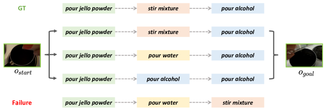
Figure 2: Visualization of diverse plans produced by our model with horizon $T=3$.

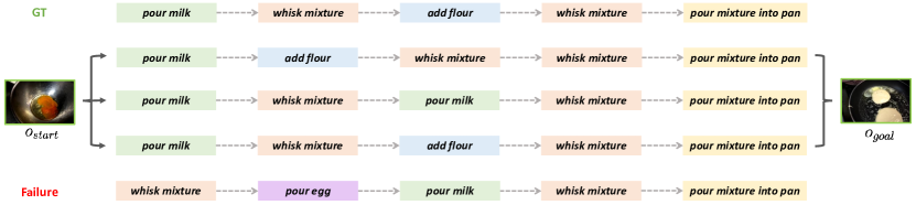
Figure 4: Visualization of diverse plans produced by our model with horizon $T=5$.

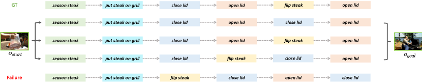
Figure 5: Visualization of diverse plans produced by our model with horizon $T=6$.

References

- [1] Jean-Baptiste Alayrac, Piotr Bojanowski, Nishant Agrawal, Josef Sivic, Ivan Laptev, and Simon Lacoste-Julien. Unsupervised learning from narrated instruction videos. In CVPR, pages 4575–4583. IEEE Computer Society, 2016.
- [2] Jing Bi, Jiebo Luo, and Chenliang Xu. Procedure planning in instructional videos via contextual modeling and model-based policy learning. In ICCV, pages 15591–15600. IEEE, 2021.
- [3] João Carreira and Andrew Zisserman. Quo vadis, action recognition? A new model and the kinetics dataset. In CVPR, pages 4724–4733. IEEE Computer Society, 2017.
- [4] Chien-Yi Chang, De-An Huang, Danfei Xu, Ehsan Adeli, Li Fei-Fei, and Juan Carlos Niebles. Procedure planning in instructional videos. In ECCV (11), volume 12356 of Lecture Notes in Computer Science, pages 334–350. Springer, 2020.
- [5] Yudong Chen and Martin J. Wainwright. Fast low-rank estimation by projected gradient descent: General statistical and algorithmic guarantees. CoRR, abs/1509.03025, 2015.
- [6] Yingpeng Deng and Lina J. Karam. Universal adversarial attack via enhanced projected gradient descent. In ICIP, pages 1241–1245. IEEE, 2020.
- [7] Prafulla Dhariwal and Alexander Quinn Nichol. Diffusion models beat gans on image synthesis. In NeurIPS, pages 8780–8794, 2021.
- [8] Nikita Dvornik, Isma Hadji, Konstantinos G. Derpanis, Animesh Garg, and Allan D. Jepson. Drop-dtw: Aligning common signal between sequences while dropping outliers. In NeurIPS, pages 13782–13793, 2021.
- [9] Nikita Dvornik, Isma Hadji, Hai Pham, Dhaivat Bhatt, Brais Martínez, Afsaneh Fazly, and Allan D. Jepson. Flow graph to video grounding for weakly-supervised multi-step localization. In ECCV (35), volume 13695 of Lecture Notes in Computer Science, pages 319–335. Springer, 2022.
- [10] Kiana Ehsani, Hessam Bagherinezhad, Joseph Redmon, Roozbeh Mottaghi, and Ali Farhadi. Who let the dogs out? modeling dog behavior from visual data. In CVPR, pages 4051–4060. Computer Vision Foundation / IEEE Computer Society, 2018.
- [11] Yazan Abu Farha and Juergen Gall. Uncertainty-aware anticipation of activities. In ICCV Workshops, pages 1197–1204. IEEE, 2019.
- [12] Chelsea Finn and Sergey Levine. Deep visual foresight for planning robot motion. In ICRA, pages 2786–2793. IEEE, 2017.
- [13] Ruohan Gao and Kristen Grauman. Co-separating sounds of visual objects. In ICCV, pages 3878–3887. IEEE, 2019.
- [14] Ian J. Goodfellow, Jean Pouget-Abadie, Mehdi Mirza, Bing Xu, David Warde-Farley, Sherjil Ozair, Aaron C. Courville, and Yoshua Bengio. Generative adversarial nets. In NIPS, pages 2672–2680, 2014.
- [15] Adrian Hauswirth, Saverio Bolognani, Gabriela Hug, and Florian Dörfler. Projected gradient descent on riemannian manifolds with applications to online power system optimization. In Allerton, pages 225–232. IEEE, 2016.
- [16] Kaiming He, Xiangyu Zhang, Shaoqing Ren, and Jian Sun. Deep residual learning for image recognition. In CVPR, pages 770–778. IEEE Computer Society, 2016.
- [17] Shawn Hershey, Sourish Chaudhuri, Daniel P. W. Ellis, Jort F. Gemmeke, Aren Jansen, R. Channing Moore, Manoj Plakal, Devin Platt, Rif A. Saurous, Bryan Seybold, Malcolm Slaney, Ron J. Weiss, and Kevin W. Wilson. CNN architectures for large-scale audio classification. In ICASSP, pages 131–135. IEEE, 2017.
- [18] Jonathan Ho, William Chan, Chitwan Saharia, Jay Whang, Ruiqi Gao, Alexey A. Gritsenko, Diederik P. Kingma, Ben Poole, Mohammad Norouzi, David J. Fleet, and Tim Salimans. Imagen video: High definition video generation with diffusion models. CoRR, abs/2210.02303, 2022.
- [19] Jonathan Ho, Ajay Jain, and Pieter Abbeel. Denoising diffusion probabilistic models. In NeurIPS, 2020.
- [20] Jonathan Ho and Tim Salimans. Classifier-free diffusion guidance. CoRR, abs/2207.12598, 2022.
- [21] Jonathan Ho, Tim Salimans, Alexey A. Gritsenko, William Chan, Mohammad Norouzi, and David J. Fleet. Video diffusion models. CoRR, abs/2204.03458, 2022.
- [22] Michael Janner, Yilun Du, Joshua B. Tenenbaum, and Sergey Levine. Planning with diffusion for flexible behavior synthesis. In ICML, volume 162 of Proceedings of Machine Learning Research, pages 9902–9915. PMLR, 2022.
- [23] Diederik P. Kingma and Jimmy Ba. Adam: A method for stochastic optimization. In ICLR (Poster), 2015.
- [24] Diederik P. Kingma, Tim Salimans, Ben Poole, and Jonathan Ho. Variational diffusion models. CoRR, abs/2107.00630, 2021.
- [25] Xiang Lisa Li, John Thickstun, Ishaan Gulrajani, Percy Liang, and Tatsunori B. Hashimoto. Diffusion-lm improves controllable text generation. CoRR, abs/2205.14217, 2022.
- [26] Chen Liang, Wenguan Wang, Tianfei Zhou, and Yi Yang. Visual abductive reasoning. In CVPR, pages 15544–15554. IEEE, 2022.
- [27] Antoine Miech, Dimitri Zhukov, Jean-Baptiste Alayrac, Makarand Tapaswi, Ivan Laptev, and Josef Sivic. Howto100m: Learning a text-video embedding by watching hundred million narrated video clips. In ICCV, pages 2630–2640. IEEE, 2019.
- [28] Diganta Misra. Mish: A self regularized non-monotonic neural activation function. CoRR, abs/1908.08681, 2019.
- [29] Alexander Quinn Nichol and Prafulla Dhariwal. Improved denoising diffusion probabilistic models. In ICML, volume 139 of Proceedings of Machine Learning Research, pages 8162–8171. PMLR, 2021.
- [30] Olaf Ronneberger, Philipp Fischer, and Thomas Brox. U-net: Convolutional networks for biomedical image segmentation. In MICCAI (3), volume 9351 of Lecture Notes in Computer Science, pages 234–241. Springer, 2015.
- [31] Jascha Sohl-Dickstein, Eric A. Weiss, Niru Maheswaranathan, and Surya Ganguli. Deep unsupervised learning using nonequilibrium thermodynamics. In ICML, volume 37 of JMLR Workshop and Conference Proceedings, pages 2256–2265. JMLR.org, 2015.
- [32] Jiaming Song, Chenlin Meng, and Stefano Ermon. Denoising diffusion implicit models. CoRR, abs/2010.02502, 2020.
- [33] Aravind Srinivas, Allan Jabri, Pieter Abbeel, Sergey Levine, and Chelsea Finn. Universal planning networks: Learning generalizable representations for visuomotor control. In ICML, volume 80 of Proceedings of Machine Learning Research, pages 4739–4748. PMLR, 2018.
- [34] Jiankai Sun, De-An Huang, Bo Lu, Yun-Hui Liu, Bolei Zhou, and Animesh Garg. Plate: Visually-grounded planning with transformers in procedural tasks. IEEE Robotics Autom. Lett., 7(2):4924–4930, 2022.
- [35] Yansong Tang, Dajun Ding, Yongming Rao, Yu Zheng, Danyang Zhang, Lili Zhao, Jiwen Lu, and Jie Zhou. COIN: A large-scale dataset for comprehensive instructional video analysis. In CVPR, pages 1207–1216. Computer Vision Foundation / IEEE, 2019.
- [36] Guy Tevet, Sigal Raab, Brian Gordon, Yonatan Shafir, Daniel Cohen-Or, and Amit H. Bermano. Human motion diffusion model. CoRR, abs/2209.14916, 2022.
- [37] Hugo Touvron, Piotr Bojanowski, Mathilde Caron, Matthieu Cord, Alaaeldin El-Nouby, Edouard Grave, Armand Joulin, Gabriel Synnaeve, Jakob Verbeek, and Hervé Jégou. Resmlp: Feedforward networks for image classification with data-efficient training. CoRR, abs/2105.03404, 2021.
- [38] Ashish Vaswani, Noam Shazeer, Niki Parmar, Jakob Uszkoreit, Llion Jones, Aidan N. Gomez, Lukasz Kaiser, and Illia Polosukhin. Attention is all you need. In NIPS, pages 5998–6008, 2017.
- [39] Andrew J. Viterbi. Error bounds for convolutional codes and an asymptotically optimum decoding algorithm. IEEE Trans. Inf. Theory, 13(2):260–269, 1967.
- [40] Yuxin Wu and Kaiming He. Group normalization. In ECCV (13), volume 11217 of Lecture Notes in Computer Science, pages 3–19. Springer, 2018.
- [41] Dongchao Yang, Jianwei Yu, Helin Wang, Wen Wang, Chao Weng, Yuexian Zou, and Dong Yu. Diffsound: Discrete diffusion model for text-to-sound generation. CoRR, abs/2207.09983, 2022.
- [42] He Zhao, Isma Hadji, Nikita Dvornik, Konstantinos G. Derpanis, Richard P. Wildes, and Allan D. Jepson. Piv: Probabilistic procedure planning from instructional videos with weak supervision. In CVPR, pages 2928–2938. IEEE, 2022.
- [43] Wenliang Zhao, Yongming Rao, Yansong Tang, Jie Zhou, and Jiwen Lu. Videoabc: A real-world video dataset for abductive visual reasoning. IEEE Trans. Image Process., 31:6048–6061, 2022.
- [44] Dimitri Zhukov, Jean-Baptiste Alayrac, Ramazan Gokberk Cinbis, David F. Fouhey, Ivan Laptev, and Josef Sivic. Cross-task weakly supervised learning from instructional videos. In CVPR, pages 3537–3545. Computer Vision Foundation / IEEE, 2019.