On the tightness of information-theoretic bounds on generalization error of learning algorithms

Abstract

A recent line of works, initiated by [1] and [2], has shown that the generalization error of a learning algorithm can be upper bounded by information measures. In most of the relevant works, the convergence rate of the expected generalization error is in the form of $O(\sqrt{\lambda/n})$ where $\lambda$ is some information-theoretic quantities such as the mutual information or conditional mutual information between the data and the learned hypothesis. However, such a learning rate is typically considered to be “slow", compared to a “fast rate" of $O(\lambda/n)$ in many learning scenarios. In this work, we first show that the square root does not necessarily imply a slow rate, and a fast rate result can still be obtained using this bound under appropriate assumptions. Furthermore, we identify the critical conditions needed for the fast rate generalization error, which we call the $(\eta,c)$-central condition. Under this condition, we give information-theoretic bounds on the generalization error and excess risk, with a fast convergence rate for specific learning algorithms such as empirical risk minimization and its regularized version. Finally, several analytical examples are given to show the effectiveness of the bounds.

I Introduction

The generalization error of a learning algorithm lies in the core analysis of the statistical learning theory, and the estimation of which becomes remarkably crucial. Conventionally, many bounding techniques are proposed under different conditions and assumptions. To name a few, Vapnik [3], Vapnik and Chervonenkis [4] proposed VC-dimension which describes the richness of a hypothesis class for generalization ability. Bousquet and Elisseeff [5] introduced a strong notion called “algorithmic stability" for bounding the generalization error, to examine where a single training sample can largely affect the generalization error. McAllester [6] investigated the bound under the Bayes framework by imposing the prior distribution over the hypothesis space. Xu and Mannor [7] developed another notion, namely robustness for the generalization. Unlike stability, the robustness conveys geometric intuition in terms of the geometric distance between instances and it can be extended to non-standard setups such as Markov chain or quantile loss, facilitating new bounds on generalization. However, most bounds mentioned above are only concerned with the hypothesis or the algorithm solely. For example, VC-dimension methods care about the worst-case bound which only depends on the hypothesis space. The stability methods only specify the properties of learning algorithms but do not require additional assumptions on hypothesis space. To fully characterize the intrinsic nature of a learning problem, it is shown in some recent works that the generalization error can be upper bounded using the information-theoretic quantities [2, 1] and the bound usually takes the following form:

$$\mathbb{E}_{W\mathcal{S}_{n}}[\mathcal{E}(W,\mathcal{S}_{n})]\leq\sqrt{\frac{cI(W;\mathcal{S}_{n})}{n}},$$ (1)

where the expectation is taken w.r.t. the joint distribution of $W$ and $\mathcal{S}_{n}$ induced by some algorithm $\mathcal{A}$. Here, $\mathcal{E}(w,\mathcal{S}_{n})$ denotes the generalization error (properly defined in (3) in Section II) for a given hypothesis $w$ and data sample $\mathcal{S}_{n}=(Z_{i})_{i=1,\cdots,n}$, and $I(W;\mathcal{S}_{n})$ denotes the mutual information between the hypothesis and data sample, and $c$ is some positive constant. In particular, if the loss function is $\sigma$-sub-Gaussian under the distribution $P_{W}\otimes P_{Z}$, $c$ is equal to $2\sigma^{2}$. By introducing the mutual information, such a bound gives a data-algorithm dependent bound that can recover the previous results in terms of VC dimension [2], algorithmic stability [8], differential privacy [9] under mild conditions. Further, as pointed out by [10], the information-theoretic upper bound could be substantially tighter than the traditional bounds if we could exploit specific properties of the learning algorithm.

However, there are mainly two issues recognized from this bound. The first problem is that the convergence rate is usually $O(\sqrt{I(W;\mathcal{S}_{n})/n})$, and if the mutual information is bounded by some constant, the bound is sub-optimal in some learning scenarios. The second issue is that the mutual information term can be arbitrarily large for deterministic algorithms [11, 12]. The latter can be addressed by introducing ghost samples [9] or using random subset methods [11, 13, 14]. Only a few works are dedicated to the former problem. In this work, we develop a general framework for the fast rate bounds using the mutual information following this line of works [15, 16, 12] and the contributions are listed as follows.

• We argue that the square root sign in (1) does not necessarily imply a slow rate. Specifically, we show that the fast rate is still achievable using the same bound, by making a slight change in the assumption, where the sub-Gaussian condition is assumed on the excess risk instead of on the loss function. Then the fast rate (e.g., $\frac{\lambda}{n}$ where $\lambda$ is the sample-wise information measure that we will specify in the Section II) is attainable if $\sigma^{2}$ has the same order as the excess risk w.r.t. the sample size, which could address the two issues simultaneously. To demonstrate the tightness of our proposed upper bound, we also propose a matching lower bound that has a similar form and the same convergence rate as the upper bound in specific learning setups.

• Inspired by the analysis under the sub-Gaussian case, we identify the critical assumptions needed for a more general fast-rate learning framework, which we call $(\eta,c)$-central condition, for the excess risk. Compared with typical mutual information bounds, the convergence rate of the novel bound has a cleaner and possibly more general presentation, which also improves from $O(\sqrt{\lambda/n})$ to $O(\lambda/n)$ under some widely used algorithms such as empirical risk minimization (ERM).

• Furthermore, our results are extended to regularized ERM algorithms, and intermediate rates could be achieved with the relaxed $(v,c)$-central condition. The fast rate results are confirmed for a few simple regression and classification examples analytically or numerically, showing the effectiveness of the proposed bounds.

II Problem formulation

Consider a dataset $\mathcal{S}_{n}=\left(z_{1},z_{2},\cdots,z_{n}\right)$ where each instance $z_{i}$ is i.i.d. drawn from some distribution $\mu$, we would like to learn a hypothesis $w$ that exploits the properties of $\mathcal{S}_{n}$, with the aim of making predictions for previously unseen new data correctly. The choice of $w$ is performed within a set of member functions $\mathcal{W}$ with the possibly randomised algorithm $\mathcal{A}:\mathcal{Z}^{n}\rightarrow\mathcal{W}$ and we define the corresponding loss function $\ell:\mathcal{W}\times\mathcal{Z}\rightarrow\mathbb{R}$. Particularly if we consider the supervised learning problem, we can write $\mathcal{Z}=\mathcal{X}\times\mathcal{Y}$ and $z_{i}=(x_{i},y_{i})$ as a feature-label pair. Then the hypothesis $w:\mathcal{X}\rightarrow\mathcal{Y}$ can be regarded as a predictor for the input sample. We will call $(\mu,\ell,\mathcal{W},\mathcal{A})$ a learning tuple. In a typical statistical learning problem, one may wish to minimize the expected loss function $L_{\mu}(w)=E_{z\sim\mu}[\ell(w,z)]$. However, as the underlying distribution $\mu$ is usually unknown in practice, one may wish to learn $w$ by some learning principle, for example, one typical way is minimizing the empirical risk induced by the dataset $\mathcal{S}_{n}$, denoted as $w_{{\sf{ERM}}}$, such that

$$w_{{\sf{ERM}}}=\operatorname*{argmin}_{w\in\mathcal{W}}\frac{1}{n}\sum_{i=1}^{n}\ell(w,z_{i}),$$ (2)

which will be employed as a predictor for the new data. We point out that many of our results obtained in this paper also hold for more general algorithms other than ERM algorithm. Here we define $\hat{L}(w,\mathcal{S}_{n})=\frac{1}{n}\sum_{i=1}^{n}\ell(w,z_{i})$ as the empirical loss. To assess how this predictor performs on unseen samples, the generalization error is then introduced to evaluate whether a learner suffers from the over-fitting (or under-fitting). For any $w\in\mathcal{W}$, we define the generalization error as

$$\mathcal{E}(w,\mathcal{S}_{n}):=\mathbb{E}_{Z\sim\mu}[\ell(w,Z)]-\frac{1}{n}\sum_{i=1}^{n}\ell(w,z_{i}).$$ (3)

Another important metric, the excess risk, is defined as

$$\mathcal{R}(w):=\mathbb{E}_{Z\sim\mu}[\ell(w,Z)]-\mathbb{E}_{Z\sim\mu}[\ell(w^{*},Z)].$$ (4)

where the optimal hypothesis for the true risk is defined as $w^{*}$ as

$$w^{*}=\operatorname*{argmin}_{w\in\mathcal{W}}E_{Z\sim\mu}[\ell(w,Z)],$$ (5)

which is unknown in practice. The excess risk evaluates how well a hypothesis $w$ performs with respect to $w^{*}$ given the data distribution $\mu$. We also define the corresponding empirical excess risk as

$$\hat{\mathcal{R}}(w,\mathcal{S}_{n}):=\frac{1}{n}\sum_{i=1}^{n}r(w,z_{i}),$$ (6)

where $r(w,z)=\ell(w,z)-\ell(w^{*},z)$. In the sequel, we are particularly interested in bounding the expected generalization error $\mathbb{E}_{W\mathcal{S}_{n}}[\mathcal{E}(W,\mathcal{S}_{n})]$ and the excess risk $\mathbb{E}_{W}[\mathcal{R}(W)]$ for any $P_{W}$ induced by the algorithm $\mathcal{A}$.

III A Change on Assumption

III-A Existing Bounds

In this section, we first review some known results on generalization error under different assumptions on the loss function. For example, the recent advances show that under the sub-Gaussian assumption, the generalization error can be upper bounded using the information-theoretic quantities such as mutual information [2, 11, 13] or conditional mutual information [9]. The bound usually takes the following general form.

Theorem 1 (Generalization error of Generic Hypothesis[11]).

Assume that the cumulant generating function of the random variable $\ell(W,Z)-\mathbb{E}\left[\ell(W,Z)\right]$ is upper bounded by $\psi(-\lambda)$ in the interval $(b_{-},0)$ and $\psi(\lambda)$ in the interval $(0,b_{+})$ under the product distribution $P_{W}\otimes\mu$ for some $b_{-}<0$ and $b_{+}>0$ where $P_{W}$ is induced by the data distribution and the algorithm. Then the expectation of the generalization error in (3) is upper bounded as

$$\mathbb{E}_{W\mathcal{S}_{n}}\left[\mathcal{E}(W,\mathcal{S}_{n})\right]\leq\frac{1}{n}\sum_{i=1}^{n}\psi^{*-1}_{-}(I(W;Z_{i})),$$ (7)

$$-\mathbb{E}_{W\mathcal{S}_{n}}\left[\mathcal{E}(W,\mathcal{S}_{n})\right]\leq\frac{1}{n}\sum_{i=1}^{n}\psi^{*-1}_{+}(I(W;Z_{i})),$$ (8)

where we define

$$\psi^{*-1}_{-}(x) :=\inf_{\lambda\in[0,-b_{-})}\frac{x+\psi(-\lambda)}{\lambda},$$ (9)

$$\psi^{*-1}_{+}(x) :=\inf_{\lambda\in[0,b_{+})}\frac{x+\psi(\lambda)}{\lambda}.$$ (10)

For different learning tasks and data distributions, the above theorem can be specialized to sub-exponential, sub-Gamma and sub-Gaussian random variables by identifying the CGF bounding function $\psi(\lambda)$. A few concrete examples are then provided that lead to different bounds in the following. More discussions on the CGF bounding function can be found in [17, 11].

Example 1 (Sub-exponential bound).

We say $X$ is a $\left(\nu^{2},\alpha\right)$-sub-exponential random variable with parameters $\nu,\alpha>0$ if:

$$\log\mathbb{E}\left[e^{\lambda(X-\mathbb{E}[X])}\right]\leq\frac{\lambda^{2}\nu^{2}}{2},\quad\forall\lambda:|\lambda|<\frac{1}{\alpha}.$$ (11)

Assume that $\ell(W,Z)$ is ($\nu^{2}$, $\alpha$)-sub-exponential under the distribution $P_{W}\otimes\mu$ for some $\nu^{2}$ and $\alpha>0$. Then it holds that

$$\mathbb{E}_{W\mathcal{S}_{n}}\left[\mathcal{E}(W,\mathcal{S}_{n})\right]\leq\begin{cases}\frac{1}{n}\sum_{i=1}^{n}\sqrt{2\nu^{2}I(W;Z_{i})},\textup{ if }I(W;Z_{i})\leq\frac{\nu^{2}}{2\alpha^{2}}\textup{ for all }i\in[n],\\ \frac{\nu^{2}}{2\alpha}+\frac{\alpha}{n}\sum_{i=1}^{n}I(W;Z_{i}),\textup{ if }I(W;Z_{i})>\frac{\nu^{2}}{2\alpha^{2}}\textup{ for all }i\in[n].\end{cases}$$ (12)

Example 2 (Sub-Gamma bound).

We say $X$ is a ($\nu^{2},\alpha$)-sub-Gamma random variable with variance parameter $\nu^{2}$ and scale parameter $\alpha$ if:

$$\log\mathbb{E}\left[e^{\lambda(X-\mathbb{E}[X])}\right]\leq\frac{\nu^{2}\lambda^{2}}{2(1-\alpha\lambda)},\quad\forall\lambda:0<\lambda<\frac{1}{\alpha}.$$ (13)

Assume that $\ell(W,Z)$ is ($\nu^{2}$, $\alpha$)-sub-Gamma under the distribution $P_{W}\otimes\mu$ for some $\nu^{2}$ and $\alpha>0$. Then it holds that

$$\mathbb{E}_{W\mathcal{S}_{n}}\left[\mathcal{E}(W,\mathcal{S}_{n})\right]\leq\frac{1}{n}\sum_{i=1}^{n}\sqrt{2\nu^{2}I(W;Z_{i})}+\alpha I(W;Z_{i}).$$ (14)

Example 3 (Sub-Gaussian bound).

We say $X$ is a $\sigma$-sub-Gaussian random variable with variance parameter $\sigma$ if:

$$\log\mathbb{E}\left[e^{\lambda(X-\mathbb{E}[X])}\right]\leq\frac{\sigma^{2}\lambda^{2}}{2},\quad\forall\lambda\in\mathbb{R}.$$ (15)

Note that the sub-Gaussian random variable is sub-exponential random variable but not the other way around. Suppose that $\ell({W},{Z})$ is $\sigma$-sub-Gaussian under the distribution $P_{W}\otimes\mu$ where $P_{W}$ is the marginal induced the algorithm $\mathcal{A}$ and data distribution $\mu$, then

$$\mathbb{E}_{W\mathcal{S}_{n}}\left[\mathcal{E}(W,\mathcal{S}_{n})\right]\leq\frac{1}{n}\sum_{i=1}^{n}\sqrt{2\sigma^{2}I\left(W;Z_{i}\right)}.$$ (16)

Remark 1.

Throughout this section, we will focus on the case when $I(W;Z_{i})\sim O(1/n)$ in the sequel so the bound in (16) gives a convergence rate of $O(\sqrt{1/n})$ for a constant $\sigma^{2}$ for both the sub-Gaussian and sub-Gamma bounds. For a broader family of the loss function that is sub-exponential, the upper bound will even not converge if the mutual information is larger than $\frac{\sigma^{2}}{2\alpha}$ for some positive constants $\sigma$ and $\alpha$ if we refer to 12. The above assumption holds for many learning settings such as ERM in the linear regression problem [8], the Gibbs algorithm with mild assumptions [8, 2, 18, 12]. More generally, the generalization error will also decay exponentially as $n$ increases if the mutual information decays exponentially, an example of which can be found in Section V-A.

From the above result, it is usually recognized that the square root sign prevents us from the fast rate, even in the following simple Gaussian mean estimation problem considered in [11].

Example 4.

Let $\ell(w,z_{i})=(w-z_{i})^{2}$, each sample is drawn from some Gaussian distribution, $Z_{i}\sim\mathcal{N}(\mu,\sigma_{N}^{2})$. We consider the ERM algorithm that gives,

$$W_{{\sf{ERM}}}=\frac{1}{n}\sum_{i=1}^{n}Z_{i}\sim\mathcal{N}(\mu,\frac{\sigma_{N}^{2}}{n}).$$

The true generalization error can be calculated to be

$$\mathbb{E}_{W\mathcal{S}_{n}}\left[\mathcal{E}(W_{\sf{ERM}},\mathcal{S}_{n})\right]=\frac{2\sigma_{N}^{2}}{n},$$

To evaluate the upper bound in Theorem 1 for this example, we notice that for any $i$, $\ell(W,Z_{i})\sim\frac{n+1}{n}\sigma_{N}^{2}\chi_{1}^{2}$ where $\chi^{2}_{1}$ denotes the chi-squared distribution with 1 degree of freedom. Hence, the cumulant generating function can be calculated as,

$$\log\mathbb{E}_{P_{W}\otimes\mu}\left[e^{\eta(\ell(W,Z)-\mathbb{E}[\ell(W,Z)])}\right]=-\sigma_{W}^{2}\eta-\frac{1}{2}\log\left(1-2\sigma_{W}^{2}\eta\right),$$

where $\eta\leq\frac{1}{2\sigma^{2}_{W}}$ and $\sigma^{2}_{W}=\frac{n+1}{n}\sigma_{N}^{2}$ to simplify the notation. In this case, it can be proved that,

$$-\sigma_{W}^{2}\eta-\frac{1}{2}\log\left(1-2\sigma_{W}^{2}\eta\right)\leq\sigma_{W}^{4}\eta^{2}.$$ (17)

We can also calculate the mutual information as

$$I(W;Z_{i})=\frac{1}{2}\log\frac{n}{n-1}.$$

With the upper bound on the CGF in (17), the bound becomes

$$\mathbb{E}_{W\mathcal{S}_{n}}\left[\mathcal{E}(W,\mathcal{S}_{n})\right]\leq\frac{\sigma_{N}^{2}}{n}\sum_{i=1}^{n}\sqrt{2\frac{(n+1)^{2}}{n^{2}}\log\frac{n}{n-1}}\leq\sigma^{2}_{N}\sqrt{\frac{2(n+1)^{2}}{(n-1)^{3}}},$$ (18)

which will be of the order $O(\frac{1}{\sqrt{n}})$ as $n$ goes to infinity, which leads to a slow convergence rate as the true generalization error is $O(\frac{1}{n})$.

III-B Bounds with A Change on the Assumption

In this section, we show that in fact the same bound can be used to derive the correct (fast) convergence rate of $O(1/n)$, with a small yet important change on the assumption. Intuitively speaking, to achieve a fast rate bound for both the generalization error and the excess risk in expectation, the output hypothesis of the learning algorithm must be “good" enough compared to the optimal hypothesis $w^{*}$. Here we encode the notion of goodness in terms of the cumulant generating function by controlling the gap between $\ell(w,Z)$ and $\ell(w^{*},Z)$. To facilitate such an idea, we make the sub-Gaussian assumption w.r.t. the excess risk and bound the generalization error as follows.

Theorem 2.

Suppose that $r({W},{Z})$ is $\sigma$-sub-Gaussian under distribution $P_{W}\otimes\mu$, then

$$\mathbb{E}_{W\mathcal{S}_{n}}\left[\mathcal{E}(W,\mathcal{S}_{n})\right]\leq\frac{1}{n}\sum_{i=1}^{n}\sqrt{2\sigma^{2}I\left(W;Z_{i}\right)}.$$ (19)

Furthermore, the excess risk can be bounded by,

$$\mathbb{E}_{W}\left[\mathcal{R}(W)\right]\leq\mathbb{E}_{W\mathcal{S}_{n}}\left[\hat{\mathcal{R}}(W,\mathcal{S}_{n})\right]+\frac{1}{n}\sum_{i=1}^{n}\sqrt{2\sigma^{2}I\left(W;Z_{i}\right)}.$$ (20)

Now we evaluate the bound in Theorem 2 for the Gaussian example. Notice that (19) is identical to (16), and the only difference between them is the assumption.

Example 5 (Continuing from Example 4).

Consider the settings in Example 4. First, we note that the expected risk minimizer $w^{*}$ is calculated as $\mu$. Then we have,

$$r(w,z_{i})=(w-z_{i})^{2}-(\mu-z_{i})^{2}.$$

The expected excess risk can be calculated as

$$\mathbb{E}_{W}[\mathcal{R}(W)]=\frac{\sigma_{N}^{2}}{n}.$$

We can then calculate the cumulant generating function as,

$$\log\mathbb{E}_{P_{W}\otimes\mu}\left[e^{\eta(r(W,Z)-\mathbb{E}[r(W,Z)])}\right]\leq\frac{4\eta^{2}\sigma_{N}^{4}}{n},$$

for any $\eta\in\mathbb{R}$ and any $n>\max\left\{\frac{(4\eta^{2}\sigma^{4}_{N}+\eta\sigma^{2}_{N})(2\eta^{2}\sigma^{4}_{N}+\eta\sigma^{2}_{N})}{\eta^{2}\sigma^{4}_{N}},4\eta^{2}\sigma_{N}^{4}+2\eta\sigma_{N}^{2}\right\}$ where the detailed calculations can be found in Appendix A-J. Hence $r(W,Z)$ is $\sqrt{\frac{8\sigma_{N}^{4}}{n}}$-sub-Gaussian under the distribution $P_{W}\otimes\mu$. Then the bound becomes,

$$\mathbb{E}_{W\mathcal{S}_{n}}\left[\mathcal{E}(W,\mathcal{S}_{n})\right]\leq\frac{\sigma_{N}^{2}}{n}\sum_{i=1}^{n}\sqrt{\frac{8}{n}\log\frac{n}{n-1}}\leq\frac{2\sqrt{2}\sigma^{2}_{N}}{n-1},$$

which is $O(1/n)$, yielding a fast rate characterization.

In light of our existing findings, the change of assumption appears to be well-justified, as we provide a thorough comprehension of the underlying reasons in Section IV-B.

IV Fast Rate Results

IV-A Bounds with Excess Risk

As observed in the results from the previous section, while our new bound is tight, it still contains a square root term in the bound. In fact, many information-theoretic bounds for generalization error [2, 8, 11, 13, 9, 1] contain the square root with the sub-Gaussian assumption, which is often seen as the obstacle to achieving fast rate results. However, as mentioned earlier, the bounds in (16) and (19) have the same structure but lead to different convergence rates. By slightly adjusting the assumption, we can obtain a fast rate result. However, this formulation of the result is still not very satisfying because both bounds contain the quantity $\sigma^{2}$ that could scale with $n$, making it hard to determine the actual convergence rate directly from the bounds. To this end, we propose a different type of bound to alleviate this drawback. To make the “fast rate" result more explicit, we first provide an alternative bound based on the sub-Gaussian assumption and the key property of the following bound is that it does not contain the square root.

Theorem 3 (Fast Rate with Sub-Gaussian Condition).

Assume that $r(W,Z)$ is $\sigma$-subgaussian under the distribution $P_{W}\otimes\mu$. Then it holds that

$$\mathbb{E}_{W\mathcal{S}_{n}}\left[\mathcal{E}(W,\mathcal{S}_{n})\right]\leq\frac{1-a_{\eta}}{a_{\eta}}\mathbb{E}_{W\mathcal{S}_{n}}[\hat{\mathcal{R}(W,\mathcal{S}_{n})}]+\frac{1}{n\eta a_{\eta}}\sum_{i=1}^{n}I\left(W;Z_{i}\right).$$ (21)

for any $0<\eta<\frac{2\mathbb{E}_{P_{W}\otimes\mu}[r(W,Z_{i})]}{\sigma^{2}}$ and $a_{\eta}=1-\frac{\eta\sigma^{2}}{2\mathbb{E}_{P_{W}\otimes\mu}[r(W,Z_{i})]}$. Furthermore, the expected excess risk is bounded by,

$$\mathbb{E}_{W}[\mathcal{R}(W)]\leq \frac{1}{a_{\eta}}\mathbb{E}_{W\mathcal{S}_{n}}[\hat{\mathcal{R}(W,\mathcal{S}_{n})}]+\frac{1}{n\eta a_{\eta}}\sum_{i=1}^{n}I\left(W;Z_{i}\right).$$

We continue to examine the bound in Theorem 3 with the Gaussian mean estimation.

Example 6.

Since the expected excess risk can be calculated as $\mathbb{E}_{W}[\mathcal{R}(W)]=\frac{\sigma_{N}^{2}}{n}$, and $r(W,Z)$ is $\sqrt{\frac{8\sigma_{N}^{4}}{n}}$-sub-Gaussian, then we require that $0<\eta<\frac{1}{2\sqrt{2}\sigma_{N}^{2}}$, which is independent of the sample size. For simplicity, we can consider the case $\eta=\frac{1}{4\sigma_{N}^{2}}$ as an example, then $a_{\eta}$ is calculated to be $\frac{1}{2}$. For any $n$ that satisfies the condition in Example 5, we have the generalization error bound,

$$\frac{1-a_{\eta}}{a_{\eta}}\mathbb{E}_{W\mathcal{S}_{n}}\left[\hat{\mathcal{R}}(W_{\sf{ERM}},\mathcal{S}_{n})\right]+\frac{1}{\eta a_{\eta}n}\sum_{i=1}^{n}I(W;Z_{i})\leq\frac{3\sigma_{N}^{2}}{n},$$

where the empirical excess risk $\mathbb{E}_{W\mathcal{S}_{n}}\left[\hat{\mathcal{R}}(W_{\sf{ERM}},\mathcal{S}_{n})\right]$ is calculated as $-\frac{\sigma^{2}_{N}}{n}$ and the bound has the rate of $O(1/n)$.

Remark 2.

Notice that both $\eta$ and $\alpha_{\eta}$ depend on the expected excess risk $\mathbb{E}_{P_{W}\otimes\mu}[r(W,Z)]$ and $\sigma^{2}$, which potentially depend on $n$ as well. Hence a more careful examination is needed. Specifically, it can be seen that if the ratio of the two quantities remains a constant independent of $n$, the fast rate result will then hold.

Ideally, we aim for a bound that does not contain extra quantities that depend on $n$, the key to such a bound is the so-called expected ($\eta,c$)-central condition (or we simply say ($\eta,c$)-central condition for short), inspired by the works [15, 19, 16, 12], which is the key condition leading to the fast rate. Similarly, we will first define the $(\eta,c)$-central condition for a non-negative random variable and use this notation to bound the generalization error with the loss function and excess risk.

Definition 1 ($(\eta,c)$-central condition).

Let ${\eta}>0$ and $0<c\leq 1$ be two constants. We say that a random variable $X$ endowed with a probability measure $P$ satisfies the $(\eta,c)$-central condition if the following inequality holds:

$$\log\mathbb{E}_{P} \left[e^{-{\eta}X}\right]\leq-c\eta\mathbb{E}_{P}\left[X\right].$$ (22)

given that $0<E_{P}[X]<\infty$.

Remark 3.

Comparing the $(\eta,c)$-central condition with the $\sigma$-sub-Gaussian condition defined as

$$\log\mathbb{E}_{P}[e^{-\eta X}]\leq-\eta\mathbb{E}_{P}[X]+\frac{\eta^{2}\sigma^{2}}{2},\forall\eta\in\mathbb{R},$$

the main difference is on the bounding terms for the CGF where the variance proxy term $\frac{\eta^{2}\sigma^{2}}{2}$ is replaced by the term $(1-c)\eta E_{P}[X]$ for a positive $\eta$. Such a condition is closely related to the Bernstein condition [20, 16, 12] and witness condition [16] that are proposed for the "fast" rate results. Different from the sub-Gaussian condition, we could eliminate the dependency of the sample size $n$ for the variance proxy $\sigma^{2}$ with the $(\eta,c)$-central condition.

Then we make the following assumption that the unexpected excess risk satisfies the $(\eta,c)$-central condition.

Assumption 1.

We assume the unexpected excess risk $r(W,Z_{i})$ satisfies the $\left(\eta,c\right)$-central condition for any $i\in[n]$, some constants $\eta>0$ and $0<c\leq 1$ under the data distribution $\mu$ and algorithm $\mathcal{A}$, e.g.,

$$\log\mathbb{E}_{P_{W}\otimes\mu} \left[e^{-{\eta}\left(\ell(W,Z)-\ell(w^{*},Z)\right)}\right]\leq-c\eta\mathbb{E}_{P_{W}\otimes\mu}\left[\ell(W,Z)-\ell(w^{*},Z)\right].$$ (23)

Compared to the conventional $\eta$-central condition [15, Def. 3.1] by setting $c=0$ in (23) as

$$\log\mathbb{E}_{P_{W}\otimes\mu} \left[e^{-{\eta}\left(\ell(w,Z)-\ell(w^{*},Z)\right)}\right]\leq 0,$$ (24)

the RHS of (23) is negative and has a tighter control than (24) of the tail behaviour for some $c>0$. Note that since the $\eta$-central condition in [15] may be strong and is usually difficult to satisfy for all $w\in\mathcal{W}$ even in some trivial examples as shown in Appendix A-J. Our proposed ($\eta,c$)-central condition is weaker in the sense that it is only required to be satisfied in expectation.

Remark 4.

With the Chernoff bound, if the loss function satisfies the $(\eta,c)$-central condition, we have the lower tail probability bound as:

$$P(r(W,Z_{i})\leq-t)\leq e^{-\eta(t+c\mathbb{E}_{P_{W}\otimes\mu}[r(W,Z_{i})])}.$$

We provide a probabilistic interpretation on the lower tail of the excess risk and this bound is particularly useful in the following two senses. On the one hand, this condition ensures that for all $\eta^{\prime}\leq\eta$, the probability that $w$ outperforms $w^{*}$ by more than $t$ is exponentially small in $t+c\mathbb{E}[r(W,Z)]$. On the other hand, this implicitly provides an upper tail bound on the excess risk probability.

With the definitions in place, we derive the fast rate bounds under the $(\eta,c)$-central condition as follows.

Theorem 4 (Fast Rate with $(\eta,c)$-central condition).

Suppose Assumption 1 is satisfied, then for all $\eta^{\prime}\in\left(0,\eta\right]$ it holds that,

$$\mathbb{E}_{W\mathcal{S}_{n}}[\mathcal{E}(W,\mathcal{S}_{n})]\leq \frac{1-c}{c}\mathbb{E}_{P_{W\mathcal{S}_{n}}}[\hat{\mathcal{R}}\left(W,\mathcal{S}_{n}\right)]+\frac{1}{c\eta^{\prime}n}\sum_{i=1}^{n}I(W;Z_{i}).$$

Furthermore, the excess risk is bounded by,

$$\mathbb{E}_{W}[\mathcal{R}(W)]\leq \frac{1}{c}\mathbb{E}_{P_{W\mathcal{S}_{n}}}[\hat{\mathcal{R}}\left(W,\mathcal{S}_{n}\right)]+\frac{1}{c\eta^{\prime}n}\sum_{i=1}^{n}I(W;Z_{i}).$$

Such a bound has a similar form with [12, Eq. (3)] which consists of the empirical excess risk and mutual information terms and the first term is negative for some algorithms such as ERM. Notice that different from the bound in Theorem 3, the bound in Theorem 4 contains constants $c$ and $\eta^{\prime}$ that do not depend on the sample size $n$. By absorbing the necessary dependence on $n$ in the definition of the ($\eta,c$)-central condition, in this case, the convergence rate will depend on the mutual information $I(W;Z_{i})$, which can achieve the convergence rate of $O({1}/{n})$ for appropriate learning problems and algorithms [18, 9, 12]. In the following, we analytically examine our bounds in Gaussian mean estimation, and we also empirically verify our bounds with a logistic regression problem in Appendix V-C.

Example 7.

We can examine whether the unexpected excess risk satisfies the $(\eta,c)$-central condition in the Gaussian mean estimation problem. It can be checked that for $n>\max\left\{\frac{(4\eta^{2}\sigma^{4}_{N}-\eta\sigma^{2}_{N})(2\eta^{2}\sigma^{4}_{N}-\eta\sigma^{2}_{N})}{\eta^{2}\sigma^{4}_{N}},4\eta^{2}\sigma_{N}^{4}-2\eta\sigma_{N}^{2}\right\}$,

$$\log\mathbb{E}_{P_{W}\otimes\mu}\left[e^{-\eta r(W,Z)}\right]\leq\frac{4\eta^{2}\sigma_{N}^{4}-\eta\sigma_{N}^{2}}{n}\leq-c\eta\frac{\sigma_{N}^{2}}{n}.$$

From the above inequality, this learning problem satisfies the $(\eta,c)$-central condition for any $0<\eta<\frac{1}{4\sigma_{N}^{2}}$ and any $c\leq 1-4\eta\sigma_{N}^{2}$, which is independent of the sample size and thus does not affect the convergence rate. Similarly, take $\eta=\frac{1}{8\sigma_{N}^{2}}$ and $c=\frac{1}{2}$, the bound becomes

$$\frac{1-c}{c}\mathbb{E}_{P_{W\mathcal{S}_{n}}}[\hat{\mathcal{R}}\left(W,\mathcal{S}_{n}\right)]+\frac{1}{c\eta^{\prime}n}\sum_{i=1}^{n}I(W;Z_{i})\leq\frac{7\sigma_{N}^{2}}{n},$$

which coincides with the bound in Example 6 and we can arrive at the fast rate since $I(W;Z_{i})\sim O(1/n)$.

It is natural to consider whether we can apply the ($\eta,c$)-central condition to the loss function and obtain fast rate results. We present the following theorem regarding the generalization error when the loss function satisfies the $(\eta,c)$-central condition.

Theorem 5 (Generalization Error Bounds with $(\eta,c)$-central condition w.r.t. the loss function).

Assume the loss function $\ell(w,z_{i})$ satisfies the $\left(\eta,c\right)$-central condition for any $i\in[n]$, some constants $\eta>0$ and $0<c\leq 1$ under the data distribution $\mu$ and algorithm $\mathcal{A}$. Then, for all $\eta^{\prime}\in\left(0,\eta\right]$, it holds that,

$$\mathbb{E}_{W\mathcal{S}_{n}}[\mathcal{E}(W,\mathcal{S}_{n})]\leq \frac{1-c}{c}\mathbb{E}_{W\mathcal{S}_{n}}[\hat{L}(W,\mathcal{S}_{n})]+\frac{\sum_{i=1}^{n}I(W;Z_{i})}{c\eta n}.$$ (25)

Remark 5.

From Theorem 5, we can evidently see the trade-off of the generalization from (25): if the empirical loss is small, we then possibly have large mutual information as $W$ fits $Z_{i}$ well, which usually leads to an over-fitting scenario and the generalization error will be large. In contrast, if the mutual information term $I(W;Z_{i})$ is small, the empirical risk tends to be large as $W$ does not exploit much knowledge from the data and hence becomes less dependent on each instance $Z_{i}$, which leads to the under-fitting scenario. If we consider an extreme case where $c=1$, the bound in (25) holds tightly as the inequality in (22) becomes equality due to Jensen’s inequality and the loss function $\ell(W,Z_{i})$ will be a constant for any $W$ and $Z_{i}$. For such a case, both L.H.S. and R.H.S. in (25) are becoming zero and the bound is tight for a constant loss. Nevertheless, this bound may not be tight as the empirical loss may not be converging with increasing sample size, as illustrated in the example below.

Example 8.

Concretely, let us again examine the Gaussian mean estimation problem. To verify the ($\eta,c$)-central condition w.r.t. the loss function, we can calculate the CGF under the distribution $P_{W}\otimes\mu$ as:

$$\log\mathbb{E}_{P_{W}\otimes\mu}[e^{-\eta\ell(W,Z)}]=-\frac{1}{2}\log(1+2\eta\frac{n+1}{n}\sigma_{N}^{2}),$$ (26)

while the expected loss can be calculated as,

$$\mathbb{E}_{P_{W}\otimes\mu}[\ell(W,Z)]=\frac{n+1}{n}\sigma_{N}^{2}.$$

Then the $(\eta,c)$-central condition can be written as:

$$-\log(1+2\eta\frac{n+1}{n}\sigma_{N}^{2})\leq-2c\eta\frac{n+1}{n}\sigma_{N}^{2}.$$

For arbitrary choice of $\eta$ and any $n\geq 1$, we can select $c$ as,

$$c=\frac{\log(1+4\eta\sigma^{2}_{N})}{4\eta\sigma^{2}_{N}}\leq\frac{\log(1+2\eta\frac{n+1}{n}\sigma_{N}^{2})}{2\eta\frac{n+1}{n}\sigma_{N}^{2}},$$

as the function $\frac{\log(1+x)}{x}$ is non-increasing for all $x>0$. The generalization error can be upper bounded by,

$$\mathbb{E}_{W\mathcal{S}_{n}}[\mathcal{E}(W,\mathcal{S}_{n})]\leq \frac{1-c}{c}\frac{n-1}{n}\sigma^{2}_{N}+\frac{1}{2c\eta(n-1)}.$$ (27)

which converges to $\frac{1-c}{c}\sigma^{2}_{N}$ with the rate of $O(\frac{1}{n})$, and the bound is not tight in this case.

Remark 6.

As can be seen from the above example, the R.H.S. of (27) does not converge to zero with $n$ increasing when $c$ and $\eta$ are chosen to be independent of the sample size $n$, which does not match the true generalization error. We can draw a comparable insight from this example as illustrated in the previous section: obtaining the fast rate result requires us to make appropriate assumptions on the unexpected excess risk $r(W,Z)$, while making assumptions under the loss function itself is not sufficient to a tight bound.

IV-B Tightness and Justification

In the following, we examine the tightness of the bound and show why $r(W,Z)$ is a more sensible choice. Technically, we use the variational representation of the KL divergence. Specifically, let $X$ be a random variable with alphabet $\mathcal{X}$ and let $P,Q$ be two probability density functions. The KL Divergence admits the following dual representation [21]:

$$D(P\|Q)=\sup_{f:\mathcal{X}\rightarrow\mathbb{R}}\mathbb{E}_{P}[f(X)]-\log\left(\mathbb{E}_{Q}\left[e^{f(X)}\right]\right).$$ (28)

and the tightness of the bound hinges on the choice of the function $f$ in (28). It is well known that under mild conditions [22], the optimal function for the Donsker-Varadhan representation in the mutual information $I(W;Z_{i})$ is achieved by $f^{\prime}(dP_{W|Z_{i}}/dP_{W}$) where $f(t)=t\log t$. We will calculate this optimizer explicitly and show that the choice of $r(W,Z_{i})$ is actually tight. To this end, we firstly calculate the densities of $P_{W}$ and $P_{W|Z_{i}}$ as: $dP_{W}=\frac{\sqrt{n}}{\sqrt{2\pi\sigma_{N}^{2}}}\exp(\frac{-(W-\mu)^{2}n}{2\sigma_{N}^{2}})$, $dP_{W|Z_{i}}=\frac{n}{\sqrt{2\pi\sigma_{N}^{2}(n-1)}}\exp(-\frac{(W-\frac{n-1}{n}\mu-\frac{1}{n}Z_{i})^{2}n^{2}}{2\sigma_{N}^{2}(n-1)}).$ Then we can calculate the optimizer as:

$$f^{\prime}(dP_{W|Z_{i}}/dP_{W}) =\log\frac{dP_{W|Z_{i}}}{dP_{W}}+1$$

$$=\frac{1}{2}\log\frac{n}{n-1}-\frac{(w-\frac{n-1}{n}\mu-\frac{1}{n}z_{i})^{2}n^{2}}{2\sigma_{N}^{2}(n-1)}+\frac{(w-\mu)^{2}n}{2\sigma_{N}^{2}}+1$$

$$=-\frac{(w-z_{i})^{2}-(\mu-z_{i})^{2}}{2\sigma_{N}^{2}}-\frac{(w-z_{i})^{2}}{2\sigma_{N}^{2}(n-1)}+1+\frac{1}{2}\log\frac{n}{n-1}$$

for fixed $w$ and $z_{i}$. The above function can be written as:

$$f^{\prime}(dP_{W|Z_{i}}/dP_{W})=-\frac{r(w,z_{i})}{2\sigma_{N}^{2}}-\frac{\ell(w,z_{i})}{2\sigma_{N}^{2}(n-1)}+\frac{1}{2}\log\frac{n}{n-1}+1.$$

The unexpected excess risk $r(w,z_{i})$ clearly appears in the optimizer with some scaling factor and shifting constant (up to a $O(\frac{1}{n})$ difference), which, however, will not affect the convergence. To rigorously show this, we state the following result.

Lemma 1.

Let $\eta=\frac{1}{2\sigma^{2}_{N}}$, the choice of the function $-r(w,z_{i})$ satisfies the following inequality:

$$\frac{n-1}{n}I(W;Z_{i})\leq\mathbb{E}_{WZ_{i}}[-\eta r(W,Z_{i})]-\log\mathbb{E}_{P_{W}\otimes\mu}[e^{-\eta r(W,Z_{i})}]\leq I(W;Z_{i}),$$

The above lemma ensures that the variational representation is essentially tight for the Gaussian example. On the other hand, the mutual information bound may not be tight if we use the loss function $\ell$ without the reference to $w^{*}$ as the equality in the variational representations may not be achieved (up to $O(\frac{1}{n})$).

Unlike typical information-theoretic results where the bounds are based on the assumption that the loss function is $\sigma$-sub-Gaussian, we assume that the excess risk is $\sigma$-sub-Gaussian. Even though the bound in (16) has exactly the same form as in (19), the key difference is that under our assumption, $\sigma$ can depend on the sample size and will converge to $0$ as the sample size increases, while this is not the case under the previous assumption as we see in Example 4. Moreover, the excess risk can be straightforwardly upper bounded as in (20).

We further argue that the choice of $-r(w,z_{i})$ leads to a tight upper bound on the generalization error by proving a matching lower bound for both the excess risk and generalization error for the Gaussian mean estimation problem.

Theorem 6 (Matching Lower Bound).

Consider the Gaussian mean estimation problem with the ERM algorithm. With a large $n$, we have:

$$\mathbb{E}_{P_{W}\otimes\mu}[r(W,Z)]\geq\frac{2\sigma^{2}_{N}}{n}\sum_{i=1}^{n}I(W;Z_{i})+\mathbb{E}_{W\mathcal{S}_{n}}[\hat{\mathcal{R}}(W,\mathcal{S}_{n})]-\frac{1}{n-1}\mathbb{E}_{W\mathcal{S}_{n}}[\mathcal{E}(W,\mathcal{S}_{n})].$$

For the generalization error, we have:

$$\mathbb{E}_{W\mathcal{S}_{n}}[\mathcal{E}(W,\mathcal{S}_{n})]\geq 2\sigma_{N}^{2}\frac{n-1}{n^{2}}\sum_{i=1}^{n}I(W;Z_{i}).$$

Remark 7.

From the above results, we observe that the sample-wise mutual information appears in both the upper and lower bounds. For the generalization error, the upper and lower bounds are matching in terms of the convergence rate with different leading constants. For the excess risk in the Gaussian mean example, the upper bound is tight since the empirical excess risk and generalization error are both of $O(\frac{1}{n})$. However, for more general learning problems, the lower bounds of the excess risk mainly depend on the empirical excess risk and the generalization error.

IV-C Connection with Other Bounds

Fast rate conditions are widely investigated under different learning frameworks and conditions [15, 19, 20, 23, 16, 24, 12]. As the most relevant work, our bound is similar to that found in [12] which applies conditional mutual information [9], but their results do not hold for unbounded losses and specifically do not hold for sub-Gaussian losses. Our result applies to general algorithms with mutual information and our assumptions are weaker since we only require the proposed conditions to hold in expectation w.r.t. $P_{W}$, instead of for all $w\in\mathcal{W}$. Our results also have the benefit of allowing the convergence factors to be further improved by using different metrics and data-processing techniques, see [17, 25, 13] for examples. Now it is instructive to compare the different assumptions used in the related works. We point out that the $(\eta,c)$-central condition is indeed the key assumption for generalizing the result of Theorem 3, which also coincides with some well-known conditions that lead to a fast rate. We firstly show that the Bernstein condition [26, 27, 28, 23] implies the $(\eta,c)$-central condition for certain $\eta$ and $c$ in the following corollary.

Corollary 1.

Let $\beta\in[0,1]$ and $B\geq 1$. For a learning tuple $(\mu,\ell,\mathcal{W},\mathcal{A})$, we say that the Bernstein condition holds if the following inequality holds for the optimal hypothesis $w^{*}$:

$${\mathbb{E}}_{P_{W}\otimes\mu} \left[\left(\ell\left(W,Z^{\prime}\right)-\ell\left(w^{*},Z^{\prime}\right)\right)^{2}\right]\leq B\left({\mathbb{E}}_{P_{W}\otimes\mu}\left[\ell\left(W,Z^{\prime}\right)-\ell\left(w^{*};Z^{\prime}\right)\right]\right)^{\beta}.$$

Then, if $\beta=1$ and $r(w,z_{i})$ is bounded by $-b$ with some $b>0$ for all $w$ and $z_{i}$, the learning tuple also satisfies $(\min(\frac{1}{b},\frac{1}{2B(e-2)}),\frac{1}{2})$-central condition.

The Bernstein condition is usually recognized as a characterization of the “easiness" of the learning problem under various $\beta$ where $\beta=1$ corresponds to the “easiest" learning case. For bounded loss functions, the Bernstein condition will automatically hold with $\beta=0$. The standard Bernstein condition requires that the inequality holds for any $w\in\mathcal{W}$, which is usually difficult to satisfy even in some trivial examples as we will see in Example 4. Different from the standard setting, we only require that the learned (randomised) hypothesis $W$ satisfy the inequality in expectation. This is a weaker but more natural condition in the sense that we do not expect any $w\in\mathcal{W}$ will work but hope that the algorithm outputs the hypothesis that performs well in average.

The second condition is the central condition with the witness condition [15, 16], which also implies the $(\eta,c)$-central condition. We say $(\mu,\ell,\mathcal{W},\mathcal{A})$ satisfies the $\eta$-central condition [15, 16] if for the optimal hypothesis $w^{*}$, the following inequality holds,

$$\mathbb{E}_{P_{W}\otimes\mu}\left[e^{-{\eta}\left(\ell(W,Z)-\ell(w^{*},Z)\right)}\right]\leq 1.$$

We also say the learning tuple $(\mu,\ell,\mathcal{W},\mathcal{A})$ satisfies the $(u,c)$-witness condition [16] if for constants $u>0$ and $c\in(0,1]$, the following inequality holds.

$$\mathbb{E}_{P_{W}\otimes\mu} [\left(\ell(W,Z)-\ell({w^{*}},Z)\right)\cdot\mathbf{1}_{\left\{\ell(W,Z)-\ell({w^{*}},Z)\leq u\right\}}]\geq c\mathbb{E}_{P_{W}\otimes\mu}\left[\ell(W,Z)-\ell({w^{*}},Z)\right],$$

where $\mathbf{1}_{\{\cdot\}}$ denotes the indicator function. Then we have the following corollary.

Corollary 2.

If the learning tuple satisfies both $\eta$-central condition and $(u,c)$-witness condition, then the learning tuple also satisfies the $(\eta^{\prime},\frac{c-\frac{c\eta^{\prime}}{\eta}}{\eta^{\prime}u+1})$-central condition for any $0<\eta^{\prime}<\eta$.

The standard $\eta$-central condition is a key condition for proving the fast rate [15, 19, 16]. Some examples are exponential concave loss functions (including log-loss) with $\eta=1$ (see [19, 24] for examples) and bounded loss functions with Massart noise condition with different $\eta$ [15]. Again, different from the standard central condition, we only require that it holds in expectation w.r.t. the distribution induced by the algorithm $\mathcal{A}$. The witness condition [16, Def. 12] is imposed to rule out situations in which learnability simply cannot hold. The intuitive interpretation of this condition is that we exclude bad hypothesis $w$ with negligible probability (but still can contribute to the expected loss), which we will never witness empirically.

The above two conditions are useful in the sense that they rely on the algorithm, the loss function and the data distribution, for which the verification in real learning scenarios may be difficult. To give more concrete examples, we further specify the distribution classes of the excess risk that are more general than the sub-Gaussian assumption, and we claim that our proposed condition can be applied to heavier tail distributions such as sub-exponential, and sub-Gamma families.

Corollary 3.

If $r(W,Z)$ is ($\nu^{2}$, $\alpha$)-sub-exponential under the distribution $P_{W}\otimes\mu$, then the learning tuple satisfies $(\min(\frac{1}{\alpha},\frac{\nu^{2}}{\mathbb{E}_{P_{W}\otimes\mu}[r(W,Z)]}),\frac{1}{2})$-central condition. If we plug in the corresponding $\eta$ and $c$ into the generalization error bound, we have the upper bound as

$$\mathbb{E}_{W\mathcal{S}_{n}}[\mathcal{E}(W,\mathcal{S}_{n})]\leq \mathbb{E}_{P_{W\mathcal{S}_{n}}}[\hat{\mathcal{R}}\left(W,\mathcal{S}_{n}\right)]+\frac{2}{\eta^{\prime}n}\sum_{i=1}^{n}I(W;Z_{i}).$$ (29)

for any $0<\eta^{\prime}<\min(\frac{1}{\alpha},\frac{\nu^{2}}{\mathbb{E}_{P_{W}\otimes\mu}[r(W,Z)]})$.

Corollary 4.

If $r(W,Z)$ is ($\nu^{2}$, $\alpha$)-sub-Gamma under the distribution $P_{W}\otimes\mu$, then the learning tuple satisfies $(\frac{\mathbb{E}_{P_{W}\otimes\mu}[r(W,Z)]}{\nu^{2}+\alpha\mathbb{E}_{P_{W}\otimes\mu}[r(W,Z)]},\frac{1}{2})$-central condition.

We summarize and outline all essential technical conditions in Table I, allowing for more straightforward comparisons. From the table, we can see that our proposed $(\eta,c)$-central condition coincides with many existing works such as [16] and [12] for certain choices of $c$ and $\eta$. With the bounded loss, $\beta=1$ in the Bernstein condition is equivalent to the central condition with the witness condition for fast rate, from which $(\eta,c)$-central condition follows. As an example of unbounded loss functions, the log-loss will satisfy the central and witness conditions under well-specified model [29, 16], which also consequently implies the $(\eta,c)$-central condition. As suggested by Theorem 3, Corollary 3 and Corollary 4, the sub-Gaussian, sub-exponential and sub-Gamma conditions can also satisfy the $(\eta,c)$-central condition for different parameters in the assumptions.

TABLE I: Technical Conditions Comparisons

Condition	Key Inequality
$(\eta,c)$-Central Condition	$\log\mathbb{E}\left[e^{-\eta r(W,Z)}\right]\leq-c\eta\mathbb{E}[r(W,Z)]$
Bernstein Condition with $\beta=1$	$\log\mathbb{E}\left[e^{-\eta r(W,Z)}\right]\leq-\frac{1}{2}\eta\mathbb{E}[r(W,Z)]$
Central + Witness Condition	$\log\mathbb{E}\left[e^{-\eta r(W,Z)}\right]\leq-\frac{1}{c_{u}}\eta\mathbb{E}[r(W,Z)]$
Central Condition Only	$\log\mathbb{E}\left[e^{-\eta r(W,Z)}\right]\leq 0$
Sub-Gaussian Condition	$\log\mathbb{E}\left[e^{-\eta r(W,Z)}\right]\leq-\eta\mathbb{E}[r(W,Z)]+\frac{\eta^{2}\sigma^{2}}{2}$
Sub-exponential Condition	$\log\mathbb{E}\left[e^{-\eta r(W,Z)}\right]\leq-\eta\mathbb{E}[r(W,Z)]+\frac{\eta^{2}\nu^{2}}{2}$
Sub-Gamma Condition	$\log\mathbb{E}\left[e^{-\eta r(W,Z)}\right]\leq-\eta\mathbb{E}[r(W,Z)]+\frac{\nu^{2}\lambda^{2}}{2(1-\alpha\lambda)}$

IV-D Extensions

It is essential to note that in real practice, the exact empirical risk minimization algorithms can be sometimes non-trivial to implement. A straightforward and effective alternative is the regularized ERM algorithm, which involves minimizing the empirical risk function and a regularization term simultaneously to control the complexity of the hypothesis. Moreover, the regularization term can sometimes make the ERM problem easier to solve. For example, in linear regression problems, adding a regularization term can help solve ill-posed issues when there is collinearity between input features. In this section, we further apply the learning bound in Theorem 4 to the regularized ERM algorithm with the following optimization problem:

$$w_{\sf{RERM}}=\operatorname*{argmin}_{w\in\mathcal{W}}\hat{L}(w,\mathcal{S}_{n})+\frac{\lambda}{n}g(w),$$

where $g:\mathcal{W}\rightarrow\mathbb{R}$ denotes the regularizer function and $\lambda$ is some coefficient. We define $\hat{\mathcal{R}}_{\textup{reg}}(w,\mathcal{S}_{n})=\hat{\mathcal{R}}(w,\mathcal{S}_{n})+\frac{\lambda}{n}(g(w)-g(w^{*}))$, then we have the following lemma.

Corollary 5.

Suppose Assumption 1 hold and also assume $|g(w_{1})-g(w_{2})|\leq B$ for any $w_{1}$ and $w_{2}$ in $\mathcal{W}$ with some $B>0$. Then for the regularized ERM hypothesis $W_{\sf{RERM}}$:

$$\mathbb{E}_{W}[\mathcal{R}(W_{\sf{RERM}})]\leq \frac{1}{c}\mathbb{E}_{P_{W\mathcal{S}_{n}}}[\hat{\mathcal{R}}_{\textup{reg}}\left(W_{\sf{RERM}},\mathcal{S}_{n}\right)]+\frac{\lambda B}{cn}+\frac{1}{c\eta^{\prime}n}\sum_{i=1}^{n}I(W_{\sf{RERM}};Z_{i}).$$

As $\hat{\mathcal{R}}_{\textup{reg}}(w,\mathcal{S}_{n})$ will be negative for $w_{\sf{RERM}}$, the regularized ERM algorithm can lead to the fast rate if $I(W_{\sf{RERM}};Z_{i})\sim O(1/n)$, which coincides with results in [20].

From Theorem 4, we can achieve the linear convergence rate $O(1/n)$if the mutual information between the hypothesis and data example is converging with $O(1/n)$. To further relax the $(\eta,c)$-central condition, we can also derive the intermediate rate with the order of $O(n^{-\alpha})$ for $\alpha\in[\frac{1}{2},1]$. Similar to the $v$-central condition, which is a weaker condition of the $\eta$-central condition [15, 16], we propose the $(v,c)$-central condition first and derive the intermediate rate results in Theorem 7.

Definition 2 ($(v,c)$-Central Condition).

We say that $(\mu,\ell,\mathcal{W},\mathcal{A})$ satisfies the $(\eta,c)$-central condition up to some $\epsilon>0$ if the following inequality holds for the optimal hypothesis $w^{*}$:

$$\log\mathbb{E}_{P_{W}\otimes\mu} \left[e^{-{\eta}\left(\ell(W,Z)-\ell(w^{*},Z)\right)}\right]\leq-c\eta\mathbb{E}_{P_{W}\otimes\mu}\left[\ell(W,Z)-\ell(w^{*},Z)\right]+\eta\epsilon.$$ (30)

Let $v:[0,\infty)\rightarrow[0,\infty)$ is a bounded and non-decreasing function satisfying $v(\epsilon)>0$ for all $\epsilon>0$. We say that $(\mu,\ell,\mathcal{W},\mathcal{A})$ satisfies the $(v,c)$-central condition if for all $\epsilon\geq 0$ such that (30) is satisfied with $\eta=v(\epsilon)$.

Theorem 7.

Assume the learning tuple $(\mu,\ell,\mathcal{W},\mathcal{A})$ satisfies the $\left(v,c\right)$-central condition up to $\epsilon$ for some function $v$ as defined in Def. 2 and $0<c<1$. Then it holds that for any $\epsilon\geq 0$ and any $0<\eta^{\prime}\leq v(\epsilon)$,

$$\mathbb{E}_{W\mathcal{S}_{n}}[\mathcal{E}(W,\mathcal{S}_{n})]\leq \frac{1-c}{c}\mathbb{E}_{P_{W\mathcal{S}_{n}}}[\hat{\mathcal{R}}\left(W,\mathcal{S}_{n}\right)]+\frac{1}{n}\sum_{i=1}^{n}\left(\frac{1}{\eta^{\prime}c}I(W;Z_{i})+\frac{\epsilon}{c}\right).$$

In particular, if $v(\epsilon)\asymp\epsilon^{1-\beta}$ for some $\beta\in[0,1]$, then the generalization error is bounded by,

$$\mathbb{E}_{W\mathcal{S}_{n}}[\mathcal{E}(W,\mathcal{S}_{n})]\leq \frac{1-c}{c}\mathbb{E}_{P_{W\mathcal{S}_{n}}}[\hat{\mathcal{R}}\left(W,\mathcal{S}_{n}\right)]+\frac{2}{nc}\sum_{i=1}^{n}I(W;Z_{i})^{\frac{1}{2-\beta}}.$$

Thus, the expected generalization is found to have an order of $I(W;Z_{i})^{\frac{1}{2-\beta}}$, which corresponds to the results under Bernstein’s condition [28, 23, 12].

V Examples

In this section, we present several additional examples of fast rates that satisfy the $(\eta,c)$-central condition. In certain examples, the convergence rate may be faster than $O(1/n)$, for instance, when the mutual information $I(W;Z_{i})$ exhibits an exponential convergence. In addition, we examine two supervised learning problems: linear regression, a simple problem, and logistic regression, a slightly more complicated problem, both of which demonstrate a convergence rate of $O(1/n)$. For completeness, we have also included some exceptional instances where the $(\eta,c)$-central condition is not satisfied, despite being relatively uncommon in learning problems.

V-A Gaussian Mean Estimation with Discrete $\mathcal{W}$

In the Gaussian mean estimation problem, instead of considering $\mathcal{W}=\mathbb{R}$, we now consider an example where we assume $z_{i}\sim\mathcal{N}(w,1),i=1,\cdots,n$ for some $w$ in the hypothesis space $\mathcal{W}$ that has finite elements, e.g., $\mathcal{W}=\{-1,1\}$. We assume $w=1$ is the true mean. Let the algorithm be maximum likelihood estimation, that is,

$$w_{\textup{MLE}} =\operatorname*{argmin}_{W\in\mathcal{W}}\frac{1}{n}\sum_{i=1}^{n}{(z_{i}-w)^{2}},$$ (31)

which can be viewed as the empirical risk minimization with the squared loss of $\ell(w,z)=(w-z)^{2}$. Similar to Example 9, the ERM algorithm produces the decision rule by:

$$w_{{\sf{ERM}}}=\begin{cases}1,\textup{ if }\frac{1}{n}\sum_{i=1}^{n}Z_{i}\geq 0,\\ -1,\textup{ otherwise.}\end{cases}$$

As $\frac{1}{n}\sum_{i=1}^{n}Z_{i}\sim\mathcal{N}(1,\frac{1}{n})$, we then have that,

$$P(w=1) =1-Q(\sqrt{n})\leq 1-\frac{\sqrt{n}}{1+n}\frac{1}{\sqrt{2\pi}}\exp(-n/2),$$

where $Q(\cdot)$ is the tail distribution function of the standard normal distribution. Similarly, we have,

$$P(w=-1) \leq\frac{1}{\sqrt{n}}\frac{1}{\sqrt{2\pi}}\exp(-n/2).$$

Then we can calculate the expected risk and the excess risk by,

$$\mathbb{E}_{P_{W}\otimes\mu}[\ell(W,Z)] =P(w=1)\mathbb{E}_{Z}[(Z-1)^{2}]+P(w=-1)\mathbb{E}_{Z}[(Z+1)^{2}]$$

$$=1+4Q(\sqrt{n})$$

$$\leq 1+\frac{4}{\sqrt{2\pi n}}\exp(-n/2).$$

It is easily calculated that $w^{*}=1$ in this case and

$$\mathbb{E}_{Z}[\ell(w^{*},Z)] =\mathbb{E}_{Z}[(Z-1)^{2}]=1.$$

Then the expected excess risk is calculated as,

$$\mathbb{E}_{P_{W}\otimes\mu}[\ell(W,Z)]-\mathbb{E}_{Z}[\ell(W^{*},Z)]\leq\frac{5}{\sqrt{2\pi n}}\exp(-\frac{n}{2})=O(\frac{e^{-n}}{\sqrt{n}}).$$

The expected generalization error is given by,

$$\mathbb{E}_{P_{W}\otimes\mu}[\ell(W,Z_{i})]-\frac{1}{n}\sum_{i=1}^{n}\mathbb{E}_{WZ_{i}}[\ell(W,Z_{i})] =2\mathbb{E}_{W\mathcal{S}_{n}}[W\frac{1}{n}\sum_{i=1}^{n}Z_{i}]-2\mathbb{E}_{W}[W]$$

$$=2\mathbb{E}_{\mathcal{S}_{n}}[|\frac{1}{n}\sum_{i=1}^{n}Z_{i}|]-2\mathbb{E}_{W}[W]$$

$$=2\sqrt{\frac{2}{n\pi}}\exp(-\frac{n}{2})=O(\frac{e^{-n}}{\sqrt{n}}).$$

Now we evaluate our mutual information bound and compare it to the true excess risk and generalization error. For a fixed $z_{i}$, we have,

$$P(w=1|z_{i}) =P(\frac{1}{n-1}\sum_{j\neq i}Z_{j}\geq-\frac{1}{n-1}z_{i})$$

$$=Q(\frac{z_{i}}{\sqrt{n-1}}+\sqrt{n-1}).$$

We then calculate the mutual information for a large $n$ by:

$$I(W;Z_{i}) =H(W)-H(W|Z_{i})$$

$$=h_{2}(Q(\sqrt{n}))-h_{2}(\mathbb{E}_{Z_{i}}[Q(\frac{Z_{i}}{\sqrt{n-1}}+\sqrt{n-1})])$$

$$\leq h_{2}(Q(\sqrt{n}))-h_{2}(Q(\frac{1}{\sqrt{n-1}}+\sqrt{n-1}))$$

$$=O(\frac{e^{-n}}{\sqrt{n}}),$$

where the inequality follows Jensen’s inequality with the fact that $Q$-function is locally convex for a large $n$ as $Q^{\prime\prime}(x)=\frac{x}{\sqrt{2\pi}}e^{-\frac{x^{2}}{2}}$ and $h_{2}$ is a concave function. By writing the excess risk as $r(w,z)=\ell(w,z)-\ell(w^{*},z)=(w-z)^{2}-(1-z)^{2}$, its moment generating function is calculated by:

$$\mathbb{E}_{P_{W}\otimes\mu}[e^{-\eta r(W,Z)}] =P(w=1)+P(w=-1)\mathbb{E}_{Z}[e^{-4\eta Z}]$$

$$=1-Q(\sqrt{n})+Q(\sqrt{n})\mathbb{E}_{Z}[e^{-4\eta Z}].$$

We can then calculate

$$\mathbb{E}_{Z}[e^{-4\eta Z}] =e^{8\eta^{2}-4\eta}$$

and

$$\log\mathbb{E}_{P_{W}\otimes\mu}[e^{-\eta r(W,Z)}]=\log(1-Q(\sqrt{n})+Q(\sqrt{n})\exp(8\eta^{2}-4\eta)).$$

Therefore, we can check the $(\eta,c)$-central condition with $\log(1+x)\leq x$ for any $x>-1$:

$$\log\mathbb{E}_{P_{W}\otimes\mu}[e^{-\eta r(W,Z)}] \leq Q(\sqrt{n})(e^{8\eta^{2}-4\eta}-1)$$

$$=-4c\eta Q(\sqrt{n}).$$

where we can choose $c=\frac{1-e^{8\eta^{2}-4\eta}}{4\eta}\leq 1-2\eta$ with selecting any $\eta\in(0,\frac{1}{2})$. Then the bound shows that:

$$\mathbb{E}_{W\mathcal{S}}[\mathcal{E}(W,\mathcal{S})]\leq\frac{2}{\eta n}\sum^{n}_{i=1}I(W;Z_{i})=O(\frac{e^{-n}}{\sqrt{n}}),$$

which dominantly decays exponentially. Such a bound matches the true convergence rate and this example shows that with the $(\eta,c)$-central condition, the convergence rate is dominated by the mutual information between the hypothesis and the instances.

V-B Linear Regression

We now extend the Gaussian mean estimation example to the linear regression problem where we have the instance space $\mathcal{Z}=\mathcal{X}\times\mathcal{Y}$ where $\mathcal{X}\subseteq\mathbb{R}^{d}$ represents the feature space and $\mathcal{Y}\subseteq\mathbb{R}$ represents the label space. We consider the linear regression model with the case $\mathcal{X}\subseteq\mathbb{R}$ for simplicity such that the label is generated in the following way:

$$Y_{i}=w^{*}X_{i}+\epsilon_{i}$$ (32)

where $w^{*}\in\mathbb{R}$ denotes the underlying (but unknown) hypothesis and $\epsilon_{i}$ are the noises i.i.d. drawn from some zero-mean distribution. We consider the loss function $\ell(w,z_{i})=(y_{i}-wx_{i})^{2}$. Then the ERM solution can be calculated as:

$$w_{{\sf{ERM}}}=\frac{\sum_{i=1}^{n}x_{i}y_{i}}{\sum_{i=1}^{n}x^{2}_{i}}=w^{*}+\sum_{i}\frac{x_{i}}{\sum_{i}x^{2}_{i}}\epsilon_{i}.$$

We consider the fixed design such that $x_{i}$ is not randomized where the optimal hypothesis is $w^{*}$ and we assume $x_{i}\neq x_{j}$ for $i\neq j$. Assume $\epsilon_{i}\sim\mathcal{N}(0,\sigma^{2})$, we can then calculate the expected loss over $\epsilon$ as:

$$\mathbb{E}_{Z_{i}}[\ell(w^{*},Z_{i})]=\mathbb{E}_{\epsilon_{i}}[(w^{*}x_{i}+\epsilon_{i}-w^{*}x_{i})^{2}]=\mathbb{E}_{\epsilon_{i}}[\epsilon_{i}^{2}]=\sigma^{2}.$$

The expected loss under $w_{{\sf{ERM}}}$ can be calculated as:

$$\mathbb{E}_{P_{W}\otimes Z_{i}}[\ell(W_{\sf{ERM}},Z_{i})] =\mathbb{E}_{\epsilon\otimes\epsilon^{\prime}_{i}}[(w^{*}x_{i}+\epsilon^{\prime}_{i}-W_{\sf{ERM}}x_{i})^{2}]$$

$$=\mathbb{E}_{\epsilon_{j}\otimes\epsilon^{\prime}_{i}}[(\epsilon^{\prime}_{i}-\sum_{j}\frac{x_{i}x_{j}}{\sum_{j}x^{2}_{j}}\epsilon_{j})^{2}]$$

$$=\sigma^{2}+\frac{x^{2}_{i}}{\sum_{j}x^{2}_{j}}\sigma^{2}$$

Therefore the excess risk can be calculated as:

$$\frac{1}{n}\sum_{i=1}^{n}\mathbb{E}_{P_{W}\otimes\mu}[\ell(W_{\sf{ERM}},Z_{i})]-\frac{1}{n}\sum_{i=1}^{n}\mathbb{E}_{Z_{i}}[\ell(w^{*},Z_{i})]=\frac{1}{n}\sigma^{2},$$

which scales with $O(\frac{1}{n})$. For the generalization error, we have,

$$\frac{1}{n}\sum_{i=1}^{n}\mathbb{E}_{P_{W}\otimes Z_{i}}[\ell(W_{\sf{ERM}},Z_{i})]-\frac{1}{n}\sum_{i=1}^{n}\mathbb{E}_{WZ_{i}}[\ell(W_{\sf{ERM}},Z_{i})] =\frac{1}{n}(\sigma^{2}+\frac{1}{n}\sigma^{2}-\sigma^{2}-\frac{1}{n}\sigma^{2}+2\frac{\sigma^{2}}{n})$$

$$=\frac{2}{n}\sigma^{2},$$

which also scales with $O(\frac{1}{n})$. Next, we can calculate the mutual information by:

$$I(W;Z_{i}) =h(W)-h(W|Z_{i})=\frac{1}{2}\log\frac{\sum_{j}x_{j}^{2}}{\sum_{j\backslash i}x_{j}^{2}}.$$

Then we have,

$$\frac{1}{n}\sum_{i=1}^{n}I(W;Z_{i}) \leq\frac{1}{2n}\sum_{i}\frac{x^{2}_{i}}{\sum_{j\backslash i}x^{2}_{j}}.$$

For $n>3$ and any $i$, there exists a constant $c\in(0,1)$ such that $\sum_{j\backslash i}x^{2}_{j}\geq c\sum_{j}x^{2}_{j}$ holds. Then we can further upper bound the mutual information terms by,

$$\frac{1}{n}\sum_{i=1}^{n}I(W;Z_{i}) \leq\frac{1}{2n}\sum_{i}\frac{x^{2}_{i}}{c\sum_{j}{x^{2}_{j}}}=\frac{1}{2nc},$$

which scales with $O(1/n)$. Since $\ell(W,Z_{i})$ is $(1+\frac{x^{2}_{i}}{\sum_{j}x^{2}_{j}})\sigma^{2}\chi^{2}$ distributed, we calculate the moment generating function as,

$$\mathbb{E}_{P_{W}\otimes\mu}[e^{\eta\ell(W_{\sf{ERM}},Z_{i})}] =-\frac{1}{2}\log(1-2(1+\frac{x^{2}_{i}}{\sum_{j}x^{2}_{j}})\sigma^{2}\eta).$$ (33)

Let $\sigma_{i}=(1+\frac{x^{2}_{i}}{\sum_{j}x^{2}_{j}})\sigma^{2}$. We have,

$$\mathbb{E}_{P_{W}\otimes\mu}[\exp{\eta(\ell(W_{\sf{ERM}},Z_{i})-\mathbb{E}[\ell(W_{\sf{ERM}},Z_{i})])}] \leq 2\sigma_{i}^{4}\eta^{2}.$$ (34)

Therefore, the generalization error bound becomes:

$$\frac{1}{n}\sum_{i=1}^{n}\sqrt{2\sigma^{4}_{i}I(W;Z_{i})}=\frac{1}{n}\sum_{i=1}^{n}\sqrt{2\left(\frac{\sum_{j}x^{2}_{j}+x^{2}_{i}}{\sum_{j}x^{2}_{j}}\right)^{2}\sigma^{4}I(W;Z_{i})}\leq\sqrt{(2-c)^{2}\sigma^{4}\frac{1}{nc}},$$

which scales with $O(\sqrt{\frac{1}{n}})$. If we consider the excess risk $r(W,Z_{i})$, we can calculate that,

$$\log\mathbb{E}_{P_{W}\otimes\mu}\left[\exp(-\eta r(W,Z_{i}))\right]=\frac{1}{2}\log\frac{\sum_{j}x^{2}_{j}/x^{2}_{i}}{\sum_{j}x^{2}_{j}/x^{2}_{i}-(4\eta^{2}\sigma^{4}-2\eta\sigma^{2})}\leq\frac{2\eta^{2}\sigma^{4}-\eta\sigma^{2}}{\sum_{j}x^{2}_{j}/x^{2}_{i}}\leq-c\eta\frac{\sigma^{2}x^{2}_{i}}{\sum_{j}x^{2}_{j}}.$$

Hence the $(\eta,c)$ is satisfied for $c\leq 1-2\eta\sigma^{2}$ and $\eta\leq\frac{1}{4\sigma^{2}}$. By selecting $\eta=\frac{1}{4\sigma^{2}}$ and $c=\frac{1}{2}$, the bounds for the ERM (by ignoring the empirical excess risk terms) become:

$$\mathbb{E}_{W\mathcal{S}_{n}}[\mathcal{E}(W,\mathcal{S}_{n})]\leq\frac{1}{\eta cn}\sum_{i=1}^{n}I(W;Z_{i})\leq\frac{8\sigma^{2}}{n}\sum_{i=1}^{n}I(W;Z_{i})$$

which scales with $O(\frac{1}{n})$.

V-C Logistic Regression

We apply our bound in a typical classification problem. Consider a logistic regression problem in a 2-dimensional space. For each $w\in\mathbb{R}^{2}$ and $z_{i}=(x_{i},y_{i})\in\mathbb{R}^{2}\times\{0,1\}$, the loss function is given by

$$\ell(w,z_{i}):=-(y_{i}\log(\sigma(w^{T}x_{i}))+(1-y_{i})\log(1-\sigma(w^{T}x_{i})))$$

where $\sigma(x)=\frac{1}{1+e^{-x}}$. Here each $x_{i}$ is drawn from a standard multivariate Gaussian distribution $\mathcal{N}(0,\mathbf{I}_{2})$ and Let $w^{*}=(0.5,0.5)$, then each $y_{i}$ is drawn from the Bernoulli distribution with the probability $P(Y_{i}=1|x_{i},w^{*})=\sigma(-x^{T}_{i}w^{*})$. We also restrict hypothesis space as $\mathcal{W}=\{w:\|w\|_{2}<3\}$ where $W_{{\sf{ERM}}}$ falls in this area with high probability. Since the hypothesis is bounded and under the log-loss, then the learning problem will satisfy the central and witness condition [15, 16]. Therefore, it will satisfy the $(\eta,c)$-central condition. We will evaluate the generalization error and excess risk bounds in (4). To this end, we need to estimate $\eta$, $c$ and mutual information $I(W_{{\sf{ERM}}},Z_{i})$ efficiently, hence we repeatedly generate $W_{{\sf{ERM}}}$ and $Z_{i}$ and use the empirical density for estimation. Specifically, we vary the sample size $n$ from $50$ to $400$ and for each $n$ we repeat the logistic regression algorithm 2000 times to generate a set of $W_{\sf{ERM}}$. By fixing $\eta=0.8$ as an example, we can empirically estimate the CGF and expected excess risk with the data sample and a set of ERM hypotheses, which leads to $c\approx 0.42$. It is worth noting that from the experiments, once $\eta$ is fixed, the choice of $c$ actually does not depend on the sample size $n$, which empirically confirms the ($\eta,c$)-central condition. For the mutual information, we decompose $I(W;X,Y)=I(W;Y)+P(Y=0)I(W;X|y=0)+P(Y=1)I(W;X|y=1)$ by chain rule, and the first term can be approximated using the continuous-discrete estimator[30] for mutual information and the rest terms are continuous-continuous ones[31, 32]. To demonstrate the usefulness of the results, we also compare the bounds with the true excess risk and true generalization error. The comparisons are shown in Figure 1.

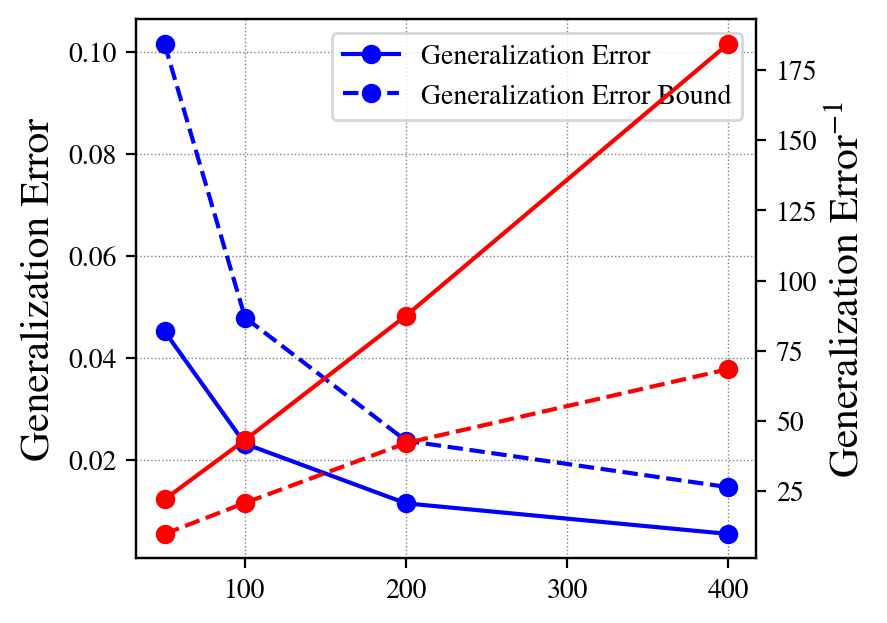
(a) Generalization Error

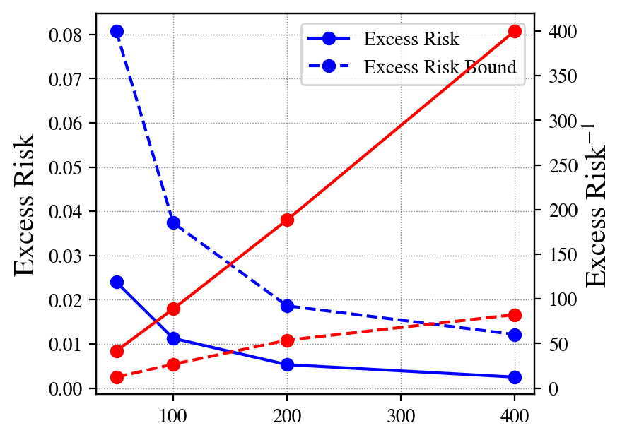
(b) Excess Risk

Figure 1: We represent the true expected generalization error in (a) and true excess risk in (b) along with their bounds in Theorem 4. Here we vary $n$ from 50 to 400. We also plot their reciprocals to show the rate w.r.t. sample size $n$. All results are derived by 2000 experimental repeats.

From the figure, we can see that both the generalization error and excess risk converge as $O(\frac{1}{n})$, and the bounds in Theorem 4 are tight, which capture the true behaviours with the same decay rate.

V-D Examples when $(\eta,c)$-central condition does not hold

There are cases where $(\eta,c)$-central condition does not hold. One instance is, when $\mathbb{E}_{P_{W}\otimes\mu}[r(W,Z)]=0$ but $\log\mathbb{E}_{P_{W}\otimes\mu}[e^{-\eta r(W,Z)}]>0$. This is an extreme case such that the algorithm yields the hypothesis that could achieve the same loss as the optimal hypothesis $w^{*}$, but a positive CGF of $r(w,z)$ under $P_{W}\otimes\mu$. For example, if there is more than one optimal hypothesis for the learning task and we denote the optimal set by $\mathcal{W}^{*}=(w^{*}_{1},w^{*}_{2},\cdots,w^{*}_{k})$ (e.g., all hypotheses in the hypothesis space are optimal), and if there is an algorithm that could produce a hypothesis distributed over $\mathcal{W}^{*}$, the expected excess risk will be zero with choosing an arbitrary optimal hypothesis from $\mathcal{W}^{*}$. But the CGF may not necessarily be zero as we have variances in the choices of the optimal hypothesis under $P_{W}$. Due to the fact that these regimes are rarely encountered in actual learning problems, the excess risk is presumed to be non-zero in order to satisfy the $(\eta,c)$-central condition. However, we still point this out to ensure the completeness of the results. In the following, we give an example where $(\eta,c)$-central condition does not hold.

Example 9 (Gaussian mean estimation with all hypotheses equally optimal).

Different from the example in V-A, we consider the zero mean Gaussian case where $Z_{i}\sim\mathcal{N}(0,1),i=1,\cdots,n$ and the same hypothesis space $\mathcal{W}=\{-1,1\}$. Intuitively speaking, unlike the previous situation, even if we have abundant data, both $1$ and $-1$ are the optimal hypothesis due to the symmetry. Mathematically, let the algorithm be maximum likelihood estimation and the ERM algorithm produces the decision rule by:

$$W_{{\sf{ERM}}}=\begin{cases}1,\textup{ if }\frac{1}{n}\sum_{i=1}^{n}Z_{i}\geq 0,\\ -1,\textup{ otherwise.}\end{cases}$$

Then the distribution of $W_{{\sf{ERM}}}$ is Bernoulli distributed with $P(w=1)=P\left(\frac{1}{n}\sum_{i=1}^{n}Z_{i}\geq 0\right).$ As $\frac{1}{n}\sum_{i=1}^{n}Z_{i}\sim\mathcal{N}(0,\frac{1}{n})$, we have that,

$$P(w=1) =P(w=-1)=\frac{1}{2}$$

due to the symmetry. Then we can calculate the expected risk and the excess risk by,

$$\mathbb{E}_{P_{W}\otimes\mu}[\ell(W,Z)] =P(w=1)\mathbb{E}_{Z}[(Z-1)^{2}]+P(w=-1)\mathbb{E}_{Z}[(Z+1)^{2}]=2.$$

It is important to note that $w^{*}$ can be either $-1$ or $1$ in this case, and

$$\mathbb{E}_{Z}[\ell(W^{*},Z)] =\mathbb{E}_{Z}[(Z-1)^{2}]=2.$$

Then the excess risk is calculated as,

$$\mathbb{E}_{P_{W}\otimes\mu}[\ell(W,Z)]-\mathbb{E}_{Z}[\ell(W^{*},Z)]=0.$$

The expected generalization error is given by,

$$\mathbb{E}_{P_{W}\otimes\mu}[\ell(W,Z_{i})]-\frac{1}{n}\sum_{i=1}^{n}\mathbb{E}_{WZ_{i}}[\ell(W,Z_{i})] =2\mathbb{E}_{\mathcal{S}_{n}}\left[\left|\frac{1}{n}\sum_{i=1}^{n}Z_{i}\right|\right]=\sqrt{\frac{8}{\pi n}}$$

due to the fact that the expectation of the absolute Gaussian r.v. with mean of $\mu$ and variance of $\sigma^{2}$ is $\sigma\sqrt{\frac{2}{\pi}}e^{-\frac{\mu^{2}}{2\sigma^{2}}}+\mu\left(1-2\Phi\left(\frac{-\mu}{\sigma}\right)\right)$. If we choose $w^{*}=1$ and the excess risk can be written as $r(w,z)=\ell(w,z)-\ell(w^{*},z)=(w-z)^{2}-(1-z)^{2}$, now we can calculate the MGF of the excess risk explicitly as:

$$\mathbb{E}_{P_{W}\otimes\mu}[e^{\eta r(W,Z)}] =P(w=1)+P(w=-1)\mathbb{E}_{Z}[e^{4\eta Z}]=\frac{1}{2}+\frac{1}{2}\mathbb{E}_{Z}[e^{4\eta Z}].$$

For the second term, we have the following:

$$\mathbb{E}_{Z}[e^{4\eta Z}] =\int^{+\infty}_{-\infty}\frac{1}{\sqrt{2\pi}}e^{-\frac{z^{2}}{2}}e^{4\eta z}dz=e^{8\eta^{2}}.$$

Finally, it yields the CGF by,

$$\log\mathbb{E}_{P_{W}\otimes\mu}[e^{\eta r(W,Z)}]=\log(\frac{1}{2}+\frac{1}{2}\exp(8\eta^{2})).$$

In this case, the $(\eta,c)$-central condition does not hold as $\log\mathbb{E}_{P_{W}\otimes\mu}[e^{-\eta r(W,Z)}]=\log(\frac{1}{2}+\frac{1}{2}\exp(8\eta^{2}))\geq 0$ for any $\eta>0$.

Example 10 (Hypothesis Selection [1]).

Let us consider a different scenario for hypothesis selection that does not satisfy the $(\eta,c)$-central condition as well. Let $\mathcal{S}=(Z_{1},Z_{2},\cdots,Z_{n})$ where $Z_{i}\in\mathbb{R}$ is a random variable with the mean of $\mu_{i}$ and $W$ to be some selection hypothesis such that $\mathcal{W}=[1:n]$. If we seek for the largest instance $Z_{i}$ in the dataset $\mathcal{S}$, we define the loss function $\ell(W,\mathcal{S})=-Z_{W}$ and simply minimising the loss function will lead to a hypothesis that produces the instance with the largest value. Then we have that $\mathbb{E}_{W\mathcal{S}}[\ell(W,\mathcal{S})]=-\mathbb{E}_{W\mathcal{S}}[Z_{W}]$ and $\mathbb{E}_{W\otimes\mathcal{S}}[\ell(W,\mathcal{S})]=-\mathbb{E}_{W\otimes\mathcal{S}}[Z_{W}]=-\mathbb{E}_{W}\mathbb{E}_{\mathcal{S}}[Z_{W}]=-\mathbb{E}_{W}[\mu_{W}]$. We can write:

$$|\mathbb{E}_{W\mathcal{S}}[\ell(W,\mathcal{S})]-\mathbb{E}_{W\otimes\mathcal{S}}[\ell(W,\mathcal{S})]|=|\mathbb{E}_{W\mathcal{S}}[Z_{W}-\mu_{W}]|.$$

We consider the ERM hypothesis $W=\operatorname*{argmin}\ell(W,\mathcal{S})=\operatorname*{argmax}_{i}Z_{i}$ and assume all $Z_{i}$ are normally distributed and have the same mean of some positive $\mu$ and variance of $\sigma^{2}$ for simplicity. Then we have that:

$$I(W;\mathcal{S})=H(W)-H(W|\mathcal{S})=H(W)=\log n.$$

Since we assume $\mu_{W}=\mu$ for all $W$, as $n$ goes to infinity, $|\mathbb{E}_{W\mathcal{S}}[Z_{W}-\mu_{W}]|=\sqrt{2\sigma^{2}\log n}$. Now we check the $(\eta,c)$-central condition w.r.t. the excess risk function $r(W,\mathcal{S})=\ell(W,\mathcal{S})-\ell(w^{*},\mathcal{S})$ where $w^{*}$ can be any index in $[1:n]$:

$$\log\mathbb{E}_{W\otimes\mathcal{S}}\left[e^{-\eta r(W,\mathcal{S})}\right]\leq-c\eta\mathbb{E}_{W\otimes\mathcal{S}}\left[r(W,\mathcal{S})\right]$$

for some $c\in[0,1]$. We can then calculate that

$$\log\mathbb{E}_{W\otimes\mathcal{S}}\left[e^{-\eta r(W,\mathcal{S})}\right]=\log\left(\frac{1}{n}+\frac{n-1}{n}\exp{\sigma^{2}\eta^{2}}\right)>0,$$

for positive $\eta$ while the expected excess risk is $\mathbb{E}_{W\otimes\mathcal{S}}\left[r(W,\mathcal{S})\right]=0$ and this contradicts to the proposed $(\eta,c)$-central condition. In both examples, we observe that the expected excess risk for the ERM hypothesis is always zero because each hypothesis in the class is optimal for the given distribution. However, the CGF could still be positive since we have stochasticity in the hypothesis derived, which is a rare occurrence in most learning scenarios, and we highlight this unique scenario for completeness.

VI Conclusion

As we demonstrate in this paper, if the sub-Gaussian assumption is made regarding the excess loss in the typical information-theoretic generalization error bounds, the square root does not necessarily prevent us from the fast rate. On top of that, we identify the key conditions that lead to the fast and intermediate rate bound in expectation. Intuitively speaking, to achieve a fast rate bound for both the generalization error in expectation, the output hypothesis of a learning algorithm must be “good" enough compared to the optimal hypothesis $w^{*}$. Here we encode the notion of goodness in terms of the CGF by controlling the gap between $\ell(w,Z)$ and $\ell(w^{*},Z)$. Further, we verify the proposed bounds and present the results analytically with examples. We remark that there is some room for future work to improve the bounds. One possible direction is to develop novel techniques for removing the empirical excess risk term in the bound for general algorithms other than ERM or regularized ERM. Additionally, in most cases, $w^{*}$ is usually not known but one could possibly seek a reference hypothesis $\hat{w}$ that could be trained from the sample and close to $w^{*}$, allowing more flexibility of the bounds in real applications.

Appendix A Proofs

A-A Proof of Theorem 2

Proof.

It is found that, due to $w^{*}$ is independent of $Z_{i}$, we have

$$\mathbb{E}_{W\mathcal{S}_{n}}[\mathcal{E}(W,\mathcal{S}_{n})]=\mathbb{E}_{W\mathcal{S}_{n}}[\mathcal{R}(W)-\hat{\mathcal{R}}(W,\mathcal{S}_{n})]=\mathbb{E}_{W\otimes\mathcal{S}_{n}}[\hat{\mathcal{R}}(W,\mathcal{S}_{n})]-\mathbb{E}_{W\mathcal{S}_{n}}[\hat{\mathcal{R}}(W,\mathcal{S}_{n})].$$ (35)

Let the distribution $P_{WZ_{i}}$ denote the joint distribution induced by $P_{W\mathcal{S}_{n}}$ with the algorihtm $P_{W|\mathcal{S}_{n}}$. With the i.i.d. assumption, we can rewrite the generalization error by,

$$\mathbb{E}_{W\mathcal{S}_{n}}[\mathcal{E}(W,\mathcal{S}_{n})]=\frac{1}{n}\sum_{i=1}^{n}\mathbb{E}_{P_{W}\otimes\mu}[r(W,Z_{i})]-\mathbb{E}_{WZ_{i}}[r(W,Z_{i})].$$ (36)

Using the KL-divergence property [2, 11] that

$$\sqrt{2\sigma^{2}D\left(P_{WZ_{i}}\|P_{W}\otimes P_{Z_{i}}\right)}\geq\mathbb{E}_{P_{W}\otimes\mu}[r(W,Z_{i})]-\mathbb{E}_{WZ_{i}}[r(W,Z_{i})]$$ (37)

under the $\sigma$-subgaussian assumption under the distribution $P_{W}\otimes\mu$. Summing up every term concludes the proof. ∎

A-B Proof of Theorem 6

Proof.

With Jensen’s inequality, we have that:

$$I(W;Z_{i}) =\mathbb{E}_{P_{WZ_{i}}}\left[-\frac{r(W,Z_{i})}{2\sigma_{N}^{2}}-\frac{(W-Z_{i})^{2}}{2\sigma^{2}_{N}(n-1)}\right]-\log\mathbb{E}_{P_{W}\otimes\mu}\left[\exp{\left(-\frac{r(W,Z_{i})}{2\sigma_{N}^{2}}-\frac{(W-Z_{i})^{2}}{2\sigma^{2}_{N}(n-1)}\right)}\right]$$

$$\leq\mathbb{E}_{P_{WZ_{i}}}\left[-\frac{r(W,Z_{i})}{2\sigma_{N}^{2}}-\frac{(W-Z_{i})^{2}}{2\sigma^{2}_{N}(n-1)}\right]-\mathbb{E}_{P_{W}\otimes\mu}\left[{-\frac{r(W,Z_{i})}{2\sigma_{N}^{2}}-\frac{(W-Z_{i})^{2}}{2\sigma^{2}_{N}(n-1)}}\right],$$ (38)

By re-arrange the inequality, we have that the following holds for all $i=1,2,\cdots,n$,

$$\mathbb{E}_{P_{W}\otimes\mu}\left[r(W,Z_{i})\right]\geq 2\sigma^{2}_{N}I(W;Z_{i})+\mathbb{E}_{P_{WZ_{i}}}[r(W,Z_{i})]+\frac{1}{n-1}(\mathbb{E}_{WZ_{i}}\left[\ell(W,Z_{i})\right]-\mathbb{E}_{P_{W}\otimes\mu}\left[\ell(W,Z_{i})\right]).$$ (39)

We complete the proof of the lower bound on the excess risk by averaging over $Z_{i}$. For the generalization error, we rewrite (38) as

$$\frac{1}{2\sigma^{2}_{N}}\frac{n}{n-1}(\mathbb{E}_{P_{W}\otimes\mu}\left[\ell(W,Z_{i})\right]-\mathbb{E}_{WZ_{i}}\left[\ell(W,Z_{i})\right])\geq I(W;Z_{i}).$$ (40)

Summing up every term for $Z_{i}$ completes the proof for the generalization error. ∎

A-C Proof of Theorem 3

Proof.

Using the Donsker-Varadhan representation of the KL divergence, we build on the following inequality for some $\eta>0$,

$$\frac{I(W;Z_{i})}{\eta}+\mathbb{E}_{P_{WZ_{i}}}\left[r(W,Z_{i})\right] \geq-\frac{1}{\eta}\log\mathbb{E}_{P_{W}\otimes\mu}[e^{-\eta(r(W,Z_{i}))}].$$ (41)

We will bound the R.H.S. using the following technique. For any $a$, we have,

$$\log\mathbb{E}_{P_{W}\otimes\mu}[e^{a\eta\mathbb{E}[r(W,Z_{i})]-\eta(r(W,Z_{i}))}] =\log\mathbb{E}_{P_{W}\otimes\mu}[e^{a\eta\mathbb{E}[r(W,Z_{i})]-\eta(r(W,Z_{i}))}]$$ (42)

$$=\log\mathbb{E}_{P_{W}\otimes\mu}[e^{\eta(\mathbb{E}[r(W,Z_{i})]-r(W,Z_{i}))+(a-1)\eta\mathbb{E}[r(W,Z_{i})]}]$$ (43)

$$\leq\frac{\sigma^{2}\eta^{2}}{2}+(a-1)\eta\mathbb{E}[r(W,Z_{i})].$$ (44)

By setting $0<a_{\eta}=1-\frac{\eta\sigma^{2}}{2\mathbb{E}[r(W,Z_{i})]}<1$, we have,

$$0<\eta<\frac{2\mathbb{E}[r(W;Z_{i})]}{\sigma^{2}},$$ (45)

and

$$\log\mathbb{E}_{P_{W}\otimes\mu}[e^{-\eta(r(W,Z_{i}))}] \leq-a_{\eta}\eta\mathbb{E}[r(W,Z_{i})].$$ (46)

We then rewrite the inequality by,

$$-\frac{1}{\eta}\log\mathbb{E}_{P_{W}\otimes\mu}[e^{-\eta(r(W,Z_{i}))}] \geq a_{\eta}\mathbb{E}[r(W,Z_{i})],$$ (47)

and we further have the following bound,

$$\frac{I(W;Z_{i})}{\eta}+\mathbb{E}_{P_{WZ_{i}}}[r(W,Z_{i})] \geq a_{\eta}\mathbb{E}_{P_{W}P_{Z_{i}}}[r(W,Z_{i})].$$ (48)

Hence,

$$\mathbb{E}_{P_{W}P_{Z_{i}}}[r(W,Z_{i})]-\mathbb{E}_{P_{WZ_{i}}}[r(W,Z_{i})]\leq\frac{I(W;Z_{i})}{\eta a_{\eta}}+\frac{1-a_{\eta}}{a_{\eta}}\mathbb{E}_{P_{WZ_{i}}}[r(W,Z_{i})].$$ (49)

Summing every term for $Z_{i}$, we have,

$$\mathbb{E}_{W\mathcal{S}_{n}}\left[\mathcal{E}(W,\mathcal{S}_{n})\right]\leq \frac{1-a_{\eta}}{a_{\eta}}\mathbb{E}_{W\mathcal{S}_{n}}[\hat{\mathcal{R}(W,\mathcal{S}_{n})}]+\frac{1}{n\eta a_{\eta}}\sum_{i=1}^{n}I\left(W;Z_{i}\right),$$ (50)

which completes the proof. ∎

A-D Proof of Theorem 5

Proof.

By the definition of mutual information, we have that for each $Z_{i}$:

$$I(W;Z_{i}) \geq-\mathbb{E}_{WZ_{i}}[\eta^{\prime}\ell(W,Z_{i})]-\log\mathbb{E}_{P_{W}\otimes\mu}\left[e^{-\eta^{\prime}\ell(W,Z_{i})}\right]$$ (51)

$$\geq-\mathbb{E}_{WZ_{i}}[\eta^{\prime}\ell(W,Z_{i})]+c\eta^{\prime}\mathbb{E}_{P_{W}\otimes\mu}[\ell(W,Z)]$$ (52)

for any $\eta^{\prime}\in(0,\eta]$. The last inequality holds due to the Jensen’s inequality and the $(\eta,c)$-central condition. By rearranging the equation, we arrive at the bound for the generalization error as:

$$\mathbb{E}_{P_{W}\otimes\mu}[\ell(W,Z_{i})]-\mathbb{E}_{WZ_{i}}[\ell(W,Z_{i})]\leq\frac{I(W;Z_{i})}{c\eta}+\frac{1-c}{c}\mathbb{E}_{WZ_{i}}[\ell(W,Z_{i})]$$ (53)

which completes the proof by:

$$\mathbb{E}_{W\mathcal{S}_{n}}[\mathcal{E}(W,\mathcal{S}_{n})]\leq\frac{\sum_{i=1}^{n}I(W;Z_{i})}{c\eta n}+\frac{1-c}{c}\mathbb{E}_{W\mathcal{S}_{n}}[\hat{L}(W,\mathcal{S}_{n})].$$ (54)

∎

A-E Proof of Corollary 1

Proof.

We first present the expected Bernstein inequality which will be the key technical lemma for the fast rate bound.

Lemma 2 (Expected Bernstein Inequality [23, 33]).

Let $U$ be a random variable bounded from below by $-b<0$ almost surely, and let $\kappa(x)=(e^{x}-x-1)/x^{2}.$ For all $\eta>0$, we have

$$\log\mathbb{E}_{U}\left[e^{\eta(\mathbb{E}[U]-U})\right]\leq\eta^{2}c_{\eta}\cdot\mathbb{E}[U^{2}],\quad\text{ for all }c_{\eta}\geq\kappa(\eta b).$$ (55)

Proof.

The proof of the lemma follows from [33] and [23]. Firstly we define $Y=-U$ which is upper bounded by $b$, then using the property that $\frac{e^{Y}-Y-1}{Y^{2}}$ in non-increasing for $Y\in\mathbb{R}$, then we define $Z=\eta Y$ such that,

$$\frac{e^{Z}-Z-1}{Z^{2}}\leq\frac{e^{\eta b}-\eta b-1}{\eta^{2}b^{2}}=\kappa(\eta b).$$ (56)

Rearranging the inequality, we then arrive at,

$$e^{Z}-Z-1\leq Z^{2}\kappa(\eta b).$$ (57)

Taking the expectation on both sides and using the fact that $\log(x+1)\leq x$ for any $x\in\mathbb{R}$, we have,

$$\log\mathbb{E}[e^{Z}]-\mathbb{E}[Z]\leq\mathbb{E}[Z^{2}]\kappa(\eta b).$$ (58)

By substituting $Z=\eta Y$, we have

$$\mathbb{E}[e^{\eta(Y-\mathbb{E}[Y])}]\leq e^{\eta^{2}\mathbb{E}[Y^{2}]\kappa(\eta b)}.$$ (59)

Define $c_{\eta}\geq\kappa(\eta b)$, it yields that

$$\mathbb{E}[e^{\eta(Y-\mathbb{E}[Y])}]\leq e^{\eta^{2}c_{\eta}\mathbb{E}[Y^{2}]}.$$ (60)

By substituting $Y=-U$, we finally have,

$$\mathbb{E}[e^{\eta(\mathbb{E}[U]-U)}]\leq e^{\eta^{2}c_{\eta}\mathbb{E}[U^{2}]},$$ (61)

which completes the proof. ∎

Using the Bernstein condition and we also assume that $r(w,z_{i})$ is lower bounded by $-b$ almost surely, we have for all $0<\eta<\frac{1}{b}$ and all $c>\frac{e^{\eta b}-\eta b-1}{\eta^{2}b^{2}}>0$, the following inequality holds:

$$e^{\eta(\mathbb{E}_{P_{W}\otimes\mu}\left[r(W,Z_{i})\right]-r(W,Z_{i}))}\leq e^{\eta^{2}c\mathbb{E}_{P_{W}\otimes\mu}\left[r^{2}(W,Z_{i})\right]}.$$ (62)

With Lemma 2, we have that for some $\beta\in[0,1]$, any $c>0$ and $\eta<\frac{1}{2Bc}$, then for all $0<\beta^{\prime}\leq\beta$ we have

$$\eta^{2}c\mathbb{E}_{P_{W}\otimes\mu}\left[r^{2}(w,Z_{i})\right]\leq\left(\frac{1}{2}\wedge\beta^{\prime}\right)\eta\left({\mathbb{E}_{P_{W}\otimes\mu}}[r(w,Z_{i})]\right)+(1-\beta^{\prime})\cdot(2Bc\eta)^{\frac{1}{1-\beta^{\prime}}}\eta.$$ (63)

Hence the equation (62) can be further bounded by

$$e^{\eta(\mathbb{E}_{P_{W}\otimes\mu}\left[r(W,Z_{i})\right]-r(W,Z_{i}))}\leq e^{\left(\frac{1}{2}\wedge\beta^{\prime}\right)\eta\left({\mathbb{E}_{P_{W}\otimes\mu}}[r(w,Z_{i})]\right)+(1-\beta^{\prime})(2Bc\eta)^{\frac{1}{1-\beta^{\prime}}}\eta}$$ (64)

for $\eta^{\prime}<\min(\frac{1}{2B(e-2)},\frac{1}{b})$. Here we can choose $c$ to be $\max_{\eta}\frac{e^{\eta b}-\eta b-1}{\eta^{2}b^{2}}=e-2$ since the function $\frac{e^{x}-x-1}{x^{2}}$ is non-decreasing in $[0,1]$. Furthermore, if $\beta^{\prime}=1$, we can rewrite (64) as,

$$e^{\eta(\mathbb{E}_{P_{W}\otimes\mu}\left[r(W,Z_{i})\right]-r(W,Z_{i}))}\leq e^{\frac{1}{2}\eta\left({\mathbb{E}_{P_{W}\otimes\mu}}[r(w,Z_{i})]\right)}$$ (65)

which completes the proof. ∎

A-F Proof of Corollary 2

Proof.

We first present the following Lemma for bounding the excess risk using the cumulant generating function.

Lemma 3 (Generalized from Lemma 13 in [16]).

Let $\bar{\eta}>0$. Assume that the expected $\eta$-strong central condition holds, and suppose further that the $(u,c)$-witness condition holds for $u>0$ and $c\in(0,1]$. Let $0<\eta^{\prime}<\eta$ and $c_{u}:=\frac{1}{c}\frac{\eta^{\prime}u+1}{1-\frac{\eta^{\prime}}{\eta}}>1$, then the following inequality holds:

$$\mathbb{E}_{P_{W}\otimes\mu}\left[r(W,Z)\right]\leq-\frac{c_{u}}{\eta^{\prime}}\log\mathbb{E}_{P_{W}\otimes\mu}\left[e^{-\eta^{\prime}r(W,Z)}\right].$$ (66)

The proof of the above lemma is similar to the proof in Appendix C.1 (page 48) in [16] by taking the expectation over the hypothesis distribution $P_{W}$, which is omitted here. Now with Lemma 3, we have that for any $0<\eta^{\prime}<\eta$,

$$\log\mathbb{E}_{P_{W}\otimes\mu}\left[e^{-\eta^{\prime}\left(r(W,Z)-\mathbb{E}_{P_{W}\otimes\mu}[r(W,Z)]\right)}\right] \leq-\frac{\eta^{\prime}}{c_{u}}\mathbb{E}_{P_{W}\otimes\mu}\left[r(W,Z)\right]+\eta^{\prime}\mathbb{E}_{P_{W}\otimes\mu}\left[r(W,Z)\right]$$ (67)

$$=(1-\frac{1}{c_{u}})\eta^{\prime}\mathbb{E}_{P_{W}\otimes\mu}\left[r(W,Z)\right].$$ (68)

Therefore, the central condition with the witness condition implies the expected $(\eta^{\prime},\frac{c-\frac{c\eta^{\prime}}{\eta}}{\eta^{\prime}u+1})$-central condition for any $0<\eta^{\prime}<\eta$. ∎

A-G Proof of Theorem 4

Proof.

Firstly we rewrite excess risk and empirical excess risk by:

$$\mathcal{R}(w) =\mathbb{E}_{Z\sim\mu}[\ell(w,Z)]-\mathbb{E}_{Z\sim\mu}[\ell(w^{*},Z)]$$

$$=\frac{1}{n}\sum_{i=1}^{n}\mathbb{E}_{Z_{i}\sim\mu}[\ell(w,Z_{i})]-\mathbb{E}_{Z_{i}\sim\mu}[\ell(w^{*},Z_{i})]$$

$$=\mathbb{E}_{\mathcal{S}_{n}}[\hat{\mathcal{R}}(w,\mathcal{S}_{n})],$$ (69)

and

$$\hat{\mathcal{R}}(w,\mathcal{S}_{n}) =\hat{L}(w,\mathcal{S}_{n})-\hat{L}(w^{*},\mathcal{S}_{n}).$$ (70)

Given any $\mathcal{S}_{n}$, the gap between the excess risk and empirical excess risk can be written as,

$$\mathcal{R}(w)-\hat{\mathcal{R}}(w,\mathcal{S}_{n})=\mathbb{E}_{\mathcal{S}_{n}}[\hat{\mathcal{R}}(w,\mathcal{S}_{n})]-\hat{\mathcal{R}}(w,\mathcal{S}_{n}).$$ (71)

We will bound the above quantity by taking the expectation w.r.t. $w$ learned from $\mathcal{S}_{n}$ by:

$$\mathbb{E}_{W\mathcal{S}_{n}}[\mathcal{E}(W)] =\mathbb{E}_{W\mathcal{S}_{n}}[\mathcal{R}(w)-\hat{\mathcal{R}}(w,\mathcal{S}_{n})]$$ (72)

$$=\mathbb{E}_{P_{W}\otimes\mathcal{S}_{n}}[\hat{\mathcal{R}}(w,\mathcal{S}_{n})]-\mathbb{E}_{W\mathcal{S}_{n}}[\hat{\mathcal{R}}(w,\mathcal{S}_{n})]$$ (73)

$$=\frac{1}{n}\sum_{i=1}^{n}\mathbb{E}_{P_{W}\otimes\mu}[r(W,Z_{i})]-\mathbb{E}_{WZ_{i}}[r(W,Z_{i})].$$ (74)

Recall that the variational representation of the KL divergence between two distributions $P$ and $Q$ defined over $\mathcal{X}$ is given as (see, e. g. [34])

$$D(P||Q)=\sup_{f}\{\mathbb{E}_{P}\left[f(X)\right]-\log\mathbb{E}_{Q}\left[e^{f(x)}\right]\},$$ (75)

where the supremum is taken over all measurable functions such that $\mathbb{E}_{Q}\left[e^{f(x)}\right]$ exists. Under the expected $(\eta,c)$-central condition, for any $0<\eta^{\prime}\leq\eta$, let $f(w,z_{i})=-\eta^{\prime}r(w,z_{i})$, we have,

$$D(P_{WZ_{i}}\|P_{W}\otimes P_{Z_{i}}) \geq\mathbb{E}_{P_{WZ_{i}}}\left[-\eta^{\prime}r(W,Z_{i})\right]-\log\mathbb{E}_{P_{W}\otimes\mu}[e^{-\eta^{\prime}(r(W,Z_{i}))}]$$

$$=\mathbb{E}_{P_{WZ_{i}}}\left[-\eta^{\prime}r(W,Z_{i})\right]-\log\mathbb{E}_{P_{W}\otimes\mu}[e^{-\eta^{\prime}(r(W,Z_{i})-\mathbb{E}_{P_{W}\otimes\mu}[r(W,Z_{i})])}]+\mathbb{E}_{P_{W}\otimes\mu}\left[\eta^{\prime}r(W,Z_{i})\right]$$

$$=\eta^{\prime}\left(\mathbb{E}_{P_{W}\otimes\mu}\left[r(W,Z_{i})\right]-\mathbb{E}_{P_{WZ_{i}}}\left[r(W,Z_{i})\right]\right)-\log\mathbb{E}_{P_{W}\otimes\mu}[e^{\eta^{\prime}(\mathbb{E}_{P_{W}\otimes\mu}[r(W,Z_{i})]-r(W,Z_{i}))}].$$ (76)

Next we will upper bound the second term $\log\mathbb{E}_{P_{W}\otimes\mu}[e^{\eta^{\prime}(\mathbb{E}_{P_{W}\otimes\mu}[r(W,Z_{i})]-r(W,Z_{i}))}]$ in R.H.S. using the expected $(\eta,c)$-central condition. From the $(\eta,c)$-central condition, we have,

$$\log\mathbb{E}_{P_{W}\otimes\mu}[e^{\eta(\mathbb{E}_{P_{W}\otimes\mu}[r(W,Z_{i})]-r(W,Z_{i}))}]\leq(1-c)\eta\mathbb{E}_{P_{W}\otimes\mu}[r(W,Z_{i})].$$ (77)

Since $\eta^{\prime}\leq\eta$, Jensen’s inequality yields:

$$\log\mathbb{E}_{P_{W}\otimes\mu}[e^{\eta^{\prime}(\mathbb{E}_{P_{W}\otimes\mu}[r(W,Z_{i})]-r(W,Z_{i}))}] =\log\mathbb{E}_{P_{W}\otimes\mu}[e^{\frac{\eta^{\prime}}{\eta}\eta(\mathbb{E}_{P_{W}\otimes\mu}[r(W,Z_{i})]-r(W,Z_{i}))}]$$ (78)

$$\leq\log\left(\mathbb{E}_{P_{W}\otimes\mu}[e^{\eta(\mathbb{E}_{P_{W}\otimes\mu}[r(W,Z_{i})]-r(W,Z_{i}))}]\right)^{\frac{\eta^{\prime}}{\eta}}$$ (79)

$$\leq\frac{\eta^{\prime}}{\eta}(1-c)\eta\mathbb{E}_{P_{W}\otimes\mu}[r(W,Z_{i})]$$ (80)

$$=\eta^{\prime}(1-c)\mathbb{E}_{P_{W}\otimes\mu}[r(W,Z_{i})].$$ (81)

Substitute (81) into (76), we arrive at,

$$I(W;Z_{i})\geq\eta^{\prime}\left(\mathbb{E}_{P_{W}\otimes\mu}\left[r(W,Z_{i})\right]-\mathbb{E}_{P_{WZ_{i}}}\left[r(W,Z_{i})\right]\right)-(1-c)\eta^{\prime}\mathbb{E}_{P_{W}\otimes\mu}[r(W,Z_{i})].$$ (82)

Divide $\eta^{\prime}$ on both side, we arrive at,

$$\frac{I(W;Z_{i})}{\eta^{\prime}}\geq\mathbb{E}_{P_{W}\otimes\mu}\left[r(W,Z_{i})\right]-\mathbb{E}_{P_{WZ_{i}}}\left[r(W,Z_{i})\right]-(1-c)\mathbb{E}_{P_{W}\otimes\mu}[r(W,Z_{i})].$$ (83)

Rearrange the equation and yields,

$$c\mathbb{E}_{P_{W}\otimes\mu}\left[r(W,Z_{i})\right]\leq\mathbb{E}_{P_{WZ_{i}}}\left[r(W,Z_{i})\right]+\frac{I(W;Z_{i})}{\eta^{\prime}}.$$ (84)

Therefore,

$$\mathbb{E}_{P_{W}\otimes\mu}\left[r(W,Z_{i})\right]-\mathbb{E}_{P_{WZ_{i}}}\left[r(W,Z_{i})\right]\leq(\frac{1}{c}-1)\left({\mathbb{E}_{P_{WZ_{i}}}}[r(w,Z_{i})]\right)+\frac{I(W;Z_{i})}{c\eta^{\prime}}.$$ (85)

Summing up every term for $Z_{i}$ and divide by $n$, we end up with,

$$\mathbb{E}_{P_{W}\otimes P_{\mathcal{S}_{n}}}\left[\hat{\mathcal{R}}(W,\mathcal{S}_{n})\right]-\mathbb{E}_{P_{W\mathcal{S}_{n}}}\left[\hat{\mathcal{R}}(W,\mathcal{S}_{n})\right]\leq (\frac{1}{c}-1)\left({\mathbb{E}_{P_{W\mathcal{S}_{n}}}}[\hat{\mathcal{R}}(W,\mathcal{S}_{n})]\right)+\frac{1}{n}\sum_{i=1}^{n}\frac{I(W;Z_{i})}{c\eta^{\prime}}.$$ (86)

Finally we completes the proof by,

$$\mathbb{E}_{W\mathcal{S}_{n}}[\mathcal{E}(W)]\leq(\frac{1}{c}-1)\left({\mathbb{E}_{P_{W\mathcal{S}_{n}}}}[\hat{\mathcal{R}}(W,\mathcal{S}_{n})]\right)+\frac{1}{n}\sum_{i=1}^{n}\frac{I(W;Z_{i})}{c\eta^{\prime}}.$$ (87)

∎

A-H Proof of Corollary 5

Proof.

We first define,

$$\hat{{L}}_{\textup{reg}}(w,\mathcal{S}_{n}):=\hat{{L}}(w,\mathcal{S}_{n})+\frac{\lambda}{n}g(w).$$ (88)

Based on Theorem 4, we can bound the excess risk for $W_{\sf{RERM}}$ by,

$$\mathbb{E}_{W}[\mathcal{R}(W_{\sf{RERM}})] \leq\frac{1}{c}\mathbb{E}_{P_{W\mathcal{S}_{n}}}[\hat{\mathcal{R}}\left(W_{\sf{RERM}},\mathcal{S}_{n}\right)]+\frac{1}{c\eta^{\prime}n}\sum_{i=1}^{n}I(W_{\sf{RERM}};Z_{i})$$ (89)

$$=\frac{1}{c}\left(\mathbb{E}_{P_{W\mathcal{S}_{n}}}[\hat{L}\left(W_{\sf{RERM}},\mathcal{S}_{n}\right)-\hat{L}\left(w^{*},\mathcal{S}_{n}\right)]\right)+\frac{1}{c\eta^{\prime}n}\sum_{i=1}^{n}I(W_{\sf{RERM}};Z_{i})$$ (90)

$$\overset{(a)}{\leq}\frac{1}{c}\left(\mathbb{E}_{P_{W\mathcal{S}_{n}}}[\hat{{L}}_{\textup{reg}}\left(W_{\sf{RERM}},\mathcal{S}_{n}\right)]-\mathbb{E}_{P_{W\mathcal{S}_{n}}}[\hat{{L}}_{\textup{reg}}\left(w^{*},\mathcal{S}_{n}\right)]\right)+\frac{\lambda B}{cn}+\frac{1}{c\eta^{\prime}n}\sum_{i=1}^{n}I(W_{\sf{RERM}};Z_{i})$$ (91)

$$=\frac{1}{c}\mathbb{E}_{P_{W\mathcal{S}_{n}}}[\hat{\mathcal{R}}_{\textup{reg}}\left(W_{\sf{RERM}},\mathcal{S}_{n}\right)]+\frac{1}{c\eta^{\prime}n}\sum_{i=1}^{n}I(W_{\sf{RERM}};Z_{i})$$ (92)

$$\overset{(b)}{\leq}\frac{\lambda B}{cn}+\frac{1}{c\eta^{\prime}n}\sum_{i=1}^{n}I(W_{\sf{RERM}};Z_{i}).$$ (93)

where (a) follows since $|g(w^{*})-g(W_{\sf{RERM}}))|\leq B$ the expected empirical risk is negative for $W_{{\sf{ERM}}}$ and (b) holds due to that $W_{\sf{RERM}}$ is the minimizer of the regularized loss. ∎

A-I Proof of Theorem 7

Proof.

We will build upon (76). With the $(v,c)$-central condition, for any $\epsilon\geq 0$ and any $0<\eta^{\prime}\leq v(\epsilon)$, the Jensen’s inequality yields:

$$\log\mathbb{E}_{P_{W}\otimes\mu}[e^{\eta^{\prime}(\mathbb{E}_{P_{W}\otimes\mu}[r(W,Z_{i})]-r(W,Z_{i}))}] =\log\mathbb{E}_{P_{W}\otimes\mu}[e^{\frac{\eta^{\prime}}{v(\epsilon)}v(\epsilon)(\mathbb{E}_{P_{W}\otimes\mu}[r(W,Z_{i})]-r(W,Z_{i}))}]$$ (94)

$$\leq\log\left(\mathbb{E}_{P_{W}\otimes\mu}[e^{v(\epsilon)(\mathbb{E}_{P_{W}\otimes\mu}[r(W,Z_{i})]-r(W,Z_{i}))}]\right)^{\frac{\eta^{\prime}}{v(\epsilon)}}$$ (95)

$$\leq\frac{\eta^{\prime}}{v(\epsilon)}\left((1-c)v(\epsilon)\mathbb{E}_{P_{W}\otimes\mu}[r(W,Z_{i})]+v(\epsilon)\epsilon\right)$$ (96)

$$=\eta^{\prime}(1-c)\mathbb{E}_{P_{W}\otimes\mu}[r(W,Z_{i})]+\eta^{\prime}\epsilon.$$ (97)

Substitute (97) into (76), we arrive at,

$$I(W;Z_{i})\geq\eta^{\prime}\left(\mathbb{E}_{P_{W}\otimes\mu}\left[r(W,Z_{i})\right]-\mathbb{E}_{P_{WZ_{i}}}\left[r(W,Z_{i})\right]\right)-(1-c)\eta^{\prime}\mathbb{E}_{P_{W}\otimes\mu}[r(W,Z_{i})]-\eta^{\prime}\epsilon.$$ (98)

Divide $\eta^{\prime}$ on both side, we arrive at,

$$\frac{I(W;Z_{i})}{\eta^{\prime}}\geq\mathbb{E}_{P_{W}\otimes\mu}\left[r(W,Z_{i})\right]-\mathbb{E}_{P_{WZ_{i}}}\left[r(W,Z_{i})\right]-(1-c)\mathbb{E}_{P_{W}\otimes\mu}[r(W,Z_{i})]-\epsilon.$$ (99)

Rearrange the equation and yields,

$$c\mathbb{E}_{P_{W}\otimes\mu}\left[r(W,Z_{i})\right]\leq\mathbb{E}_{P_{WZ_{i}}}\left[r(W,Z_{i})\right]+\frac{I(W;Z_{i})}{\eta^{\prime}}+\epsilon.$$ (100)

Therefore,

$$\mathbb{E}_{P_{W}\otimes\mu}\left[r(W,Z_{i})\right]-\mathbb{E}_{P_{WZ_{i}}}\left[r(W,Z_{i})\right]\leq(\frac{1}{c}-1)\left({\mathbb{E}_{P_{WZ_{i}}}}[r(w,Z_{i})]\right)+\frac{I(W;Z_{i})}{c\eta^{\prime}}+\frac{\epsilon}{c}.$$ (101)

Summing up every term for $Z_{i}$ and divide by $n$, we end up with,

$$\mathbb{E}_{P_{W}\otimes P_{\mathcal{S}_{n}}}\left[\hat{\mathcal{R}}(W,\mathcal{S}_{n})\right]-\mathbb{E}_{P_{W\mathcal{S}_{n}}}\left[\hat{\mathcal{R}}(W,\mathcal{S}_{n})\right]\leq (\frac{1}{c}-1)\left({\mathbb{E}_{P_{W\mathcal{S}_{n}}}}[\hat{\mathcal{R}}(W,\mathcal{S}_{n})]\right)+\frac{1}{n}\sum_{i=1}^{n}\left(\frac{I(W;Z_{i})}{c\eta^{\prime}}+\frac{\epsilon}{c}\right).$$ (102)

Finally we arrive at the following inequality:

$$\mathbb{E}_{W\mathcal{S}_{n}}[\mathcal{E}(W)]\leq(\frac{1}{c}-1)\left({\mathbb{E}_{P_{W\mathcal{S}_{n}}}}[\hat{\mathcal{R}}(W,\mathcal{S}_{n})]\right)+\frac{1}{n}\sum_{i=1}^{n}\left(\frac{I(W;Z_{i})}{c\eta^{\prime}}+\frac{\epsilon}{c}\right).$$ (103)

In particular, if $v(\epsilon)=\epsilon^{1-\beta}$ for some $\beta\in[0,1]$, then by choosing $\eta^{\prime}=v(\epsilon)$ and $\frac{I(W;Z_{i})}{c\eta^{\prime}}+\frac{\epsilon}{c}$ is optimized when $\epsilon=I(W;Z_{i})^{\frac{1}{2-\beta}}$ and the bound becomes,

$$\mathbb{E}_{W\mathcal{S}_{n}}[\mathcal{E}(W)]\leq(\frac{1}{c}-1)\left({\mathbb{E}_{P_{W\mathcal{S}_{n}}}}[\hat{\mathcal{R}}(W,\mathcal{S}_{n})]\right)+\frac{2}{nc}\sum_{i=1}^{n}I(W;Z_{i})^{\frac{1}{2-\beta}},$$ (104)

which completes the proof. ∎

A-J Calculation Details

In this section, we present the calculation details of the Gaussian mean estimation case. Let us consider the 1D-Gaussian mean estimation problem. Let $\ell(w,z_{i})=(w-z_{i})^{2}$, each sample is drawn from some Gaussian distribution, i.e., $Z_{i}\sim\mathcal{N}(\mu,\sigma_{N}^{2})$. Then the ERM algorithm arrives at,

$$W_{{\sf{ERM}}}=\frac{1}{n}\sum_{i=1}^{n}Z_{i}\sim\mathcal{N}(\mu,\frac{\sigma_{N}^{2}}{n}).$$ (105)

It can be easily calculated that the optimal $w^{*}$ satisfies:

$$w^{*}=\operatorname*{argmin}\mathbb{E}_{Z}\left[\ell(w,Z)\right]=\operatorname*{argmin}\mathbb{E}_{Z}\left[(w-Z)^{2}\right]=\mu.$$ (106)

Also it can be calculated that the expected excess risk is,

$$\mathbb{E}_{W}\left[\mathcal{R}(W_{\sf{ERM}})\right] =\mathbb{E}_{P_{W}\otimes\mu}[\ell(W_{\sf{ERM}},Z)]-\mathbb{E}_{Z}[\ell(w^{*},Z)]$$ (107)

$$=\mathbb{E}_{P_{W}\otimes\mu}[(W_{\sf{ERM}}-Z)^{2}]-\mathbb{E}_{Z}[(\mu-Z)^{2}]$$ (108)

$$=\mu^{2}+\frac{\sigma_{N}^{2}}{n}+\mu^{2}+\sigma_{N}^{2}-2\mu^{2}-\mu^{2}-\mu^{2}-\sigma_{N}^{2}+2\mu^{2}$$ (109)

$$=\frac{\sigma_{N}^{2}}{n}.$$ (110)

The corresponding empirical excess risk is given by,

$$\mathbb{E}_{W\mathcal{S}_{n}}\left[\hat{\mathcal{R}}(W_{\sf{ERM}},\mathcal{S}_{n})\right] =\mathbb{E}_{W_{\sf{ERM}}\mathcal{S}_{n}}\left[\hat{L}(W_{\sf{ERM}},\mathcal{S}_{n})-\hat{L}(w^{*},\mathcal{S}_{n})\right]$$ (111)

$$=\mathbb{E}\left[\frac{1}{n}\sum_{i=1}^{n}(W-Z_{i})^{2}-\frac{1}{n}\sum_{i=1}^{n}(\mu-Z_{i})^{2}\right]$$ (112)

$$=\mu^{2}+\frac{\sigma_{N}^{2}}{n}-\mu^{2}-2\mu^{2}-\frac{2}{n}\sigma_{N}^{2}+2\mu^{2}$$ (113)

$$=-\frac{\sigma_{N}^{2}}{n}.$$ (114)

Then it yields the expected generalization error as,

$$\mathbb{E}_{W\mathcal{S}_{n}}\left[\mathcal{E}(W_{\sf{ERM}},\mathcal{S}_{n})\right] =\mathbb{E}_{W\mathcal{S}_{n}}\left[\mathcal{R}(W_{\sf{ERM}})-\hat{\mathcal{R}}(W_{\sf{ERM}},\mathcal{S}_{n})\right]$$ (115)

$$=\frac{\sigma_{N}^{2}}{n}-(-\frac{\sigma_{N}^{2}}{n})$$ (116)

$$=\frac{2\sigma_{N}^{2}}{n}.$$ (117)

The expected loss can be calculated as,

$$\mathbb{E}_{P_{W}\otimes\mu}[\ell(W_{{\sf{ERM}}},Z)]=\frac{n+1}{n}\sigma_{N}^{2}:=\sigma_{W}^{2}.$$ (118)

Let us verify the moment generating functions for the squared loss. Since $\ell(W_{\sf{ERM}},Z)$ is $\sigma^{2}_{W}\chi^{2}_{1}$ distributed,

$$\log\mathbb{E}_{P_{W}\otimes\mu}[e^{\eta(W_{\sf{ERM}}-Z)^{2}}]=-\frac{1}{2}\log(1-2\sigma^{2}_{W}\eta).$$ (119)

Hence,

$$\log\mathbb{E}_{P_{W}\otimes\mu}[e^{\eta\left((W_{\sf{ERM}}-Z)^{2}-\mathbb{E}[(W_{\sf{ERM}}-Z)^{2}]\right)}]=-\frac{1}{2}\log(1-2\sigma^{2}_{W}\eta)-\sigma^{2}_{W}\eta.$$ (120)

It is easily to prove that for any $x\leq 0$,

$$-\frac{1}{2}\log(1-2x)-x\leq x^{2},$$ (121)

which yields,

$$\log\mathbb{E}_{P_{W}\otimes\mu}[e^{\eta\left((W_{\sf{ERM}}-Z)^{2}-\mathbb{E}[(W_{\sf{ERM}}-Z)^{2}]\right)}]=-\frac{1}{2}\log(1-2\sigma^{2}_{W}\eta)-\sigma^{2}_{W}\eta\leq\sigma_{W}^{4}\eta^{2}$$ (122)

for any $\eta<0$. Therefore, $\ell(W,Z)$ is $\sqrt{2\sigma^{4}_{W}}$-sub-Gaussian and we can only achieve the slow rate of $O(\sqrt{1/n})$.

Now we introduce $w^{*}$ in the sequel as a comparison. For a given $\eta$ and $w$, we calculate the moment generating function for the term $r(w,Z)=(w-Z)^{2}-(w^{*}-Z)^{2}$ as follows.

$$\mathbb{E}_{\mu}[e^{\eta r(w,Z)}] =\frac{1}{\sqrt{2\pi\sigma_{N}^{2}}}\int e^{-\frac{(z-\mu)^{2}}{2\sigma_{N}^{2}}}e^{\eta((w-z)^{2}-(w^{*}-z)^{2})}dz$$ (123)

$$=\frac{1}{\sqrt{2\pi\sigma_{N}^{2}}}\int\operatorname{exp}\left(-\frac{(z-\mu+2\eta\sigma_{N}^{2}(w-\mu))^{2}}{2\sigma_{N}^{2}}\right)dz\operatorname{exp}\left(-2\mu\eta(w-\mu)+2\eta^{2}\sigma_{N}^{2}(w-\mu)^{2}-\eta(\mu^{2}-w^{2})\right)$$ (124)

$$=\operatorname{exp}\left(-2\mu\eta(w-\mu)+2\eta^{2}\sigma_{N}^{2}(w-\mu)^{2}-\eta(\mu^{2}-w^{2})\right)$$ (125)

$$=\operatorname{exp}\left((2\eta^{2}\sigma_{N}^{2}+\eta)(w-\mu)^{2}\right).$$ (126)

Taking expectation over $w$ w.r.t. ERM solution, we have,

$$\mathbb{E}_{P_{W}\otimes\mu}[e^{\eta r(W,Z)}] =\mathbb{E}_{W}\left[\operatorname{exp}\left((2\eta^{2}\sigma_{N}^{2}+\eta)(w-\mu)^{2}\right)\right]$$ (127)

$$=\frac{1}{\sqrt{2\pi\frac{\sigma_{N}^{2}}{n}}}\int\operatorname{exp}\left(-\frac{(w-\mu)^{2}}{2\sigma_{N}^{2}/n}+(2\eta^{2}\sigma_{N}^{2}+\eta)(w-\mu)^{2}\right)dw$$ (128)

$$=\frac{\sqrt{\frac{1}{\frac{n}{\sigma_{N}^{2}}-(4\eta^{2}\sigma_{N}^{2}+2\eta)}\frac{n}{\sigma_{N}^{2}}}}{\sqrt{2\pi\frac{1}{\frac{n}{\sigma_{N}^{2}}-(4\eta^{2}\sigma_{N}^{2}+2\eta)}}}\int\operatorname{exp}\left(-\frac{(w-\mu)^{2}}{2}(\frac{n}{\sigma_{N}^{2}}-(4\eta^{2}\sigma_{N}^{2}+2\eta))\right)dw$$ (129)

$$=\sqrt{\frac{n}{n-(4\eta^{2}\sigma_{N}^{4}+2\eta\sigma_{N}^{2})}}.$$ (130)

Therefore for any $\eta\in\mathbb{R}$ and any $n>\max\left\{\frac{(4\eta^{2}\sigma^{4}_{N}+\eta\sigma^{2}_{N})(2\eta^{2}\sigma^{4}_{N}+\eta\sigma^{2}_{N})}{\eta^{2}\sigma^{4}_{N}},4\eta^{2}\sigma_{N}^{4}+2\eta\sigma_{N}^{2}\right\}$, we arrive at,

$$\log\mathbb{E}_{P_{W}\otimes\mu}[e^{\eta(r(W,Z)-\mathbb{E}[r(W,Z)]}] =\frac{1}{2}\log\frac{n}{n-(4\eta^{2}\sigma_{N}^{4}+2\eta\sigma_{N}^{2})}-\frac{\eta\sigma_{N}^{2}}{n}$$ (131)

$$\leq\frac{1}{2}\frac{4\eta^{2}\sigma_{N}^{4}+2\eta\sigma_{N}^{2}}{n-4\eta^{2}\sigma^{4}_{N}-2\eta\sigma^{2}_{N}}-\frac{\eta\sigma_{N}^{2}}{n}$$ (132)

$$\leq\frac{4\eta^{2}\sigma_{N}^{4}}{n}.$$ (133)

which is of the order $O(\frac{1}{n})$ and we used the fact that $\frac{a+b}{n-2a-2b}\leq\frac{2a+b}{n}$ for $n>\max\left\{\frac{(2a+b)(2a+2b)}{a},2a+2b\right\}$ with $a>0$. The mutual information can be calculated as,

$$I(W_{\sf{ERM}};Z_{i}) =h(W_{\sf{ERM}})-h(W_{\sf{ERM}}|Z_{i})$$ (134)

$$=\frac{1}{2}\log\frac{2\pi e\sigma_{N}^{2}}{n}-\frac{1}{2}\log\frac{2\pi e(n-1)\sigma_{N}^{2}}{n^{2}}$$ (135)

$$=\frac{1}{2}\log\frac{n}{n-1}$$ (136)

$$=O(\frac{1}{n}).$$ (137)

Quantity	Values/Distribution
$\mathcal{S}_{n}$	$\{Z_{1},Z_{2},\cdots,Z_{n}\}$
$Z_{i}$	$\mathcal{N}(\mu,\sigma_{N}^{2})$
$\ell(w,z)$	$(w-z)^{2}$
$\hat{L}(w,\mathcal{S}_{n})$	$\frac{1}{n}\sum_{i=1}^{n}\ell(w,z_{i})$
$L(w)$	$\mathbb{E}_{Z}\left[\ell(w,Z)\right]$
$W_{\sf{ERM}}$	$\mathcal{N}(\mu,\frac{\sigma_{N}^{2}}{n})$
$w^{*}$	$\mu$
$r(w,z)$	$(w-z)^{2}-(w^{*}-z)^{2}$
$\mathcal{R}(w)$	$L(w)-L(w^{*})$
$\hat{\mathcal{R}}(w,\mathcal{S}_{n})$	$\hat{L}(w)-\hat{L}(w^{*})$
$\mathcal{E}(w,\mathcal{S}_{n})$	$L(w)-\frac{1}{n}\sum_{i=1}^{n}\ell(w,z_{i})$
$M_{Z}[r(w,Z)]$	$-\frac{1}{\eta}\log\mathbb{E}_{Z}\left[e^{-\eta r(w,Z)}\right]$
$M_{P_{W}\otimes\mu}[r(w,Z)]$	$-\frac{1}{\eta}\log\mathbb{E}_{P_{W}\otimes\mu}\left[e^{-\eta r(W,Z)}\right]$
$\mathbb{E}_{W\mathcal{S}_{n}}\left[\hat{\mathcal{R}}(W_{\sf{ERM}},\mathcal{S}_{n})\right]$	$-\frac{\sigma_{N}^{2}}{n}$
$\mathbb{E}_{W}\left[\mathcal{R}(W_{\sf{ERM}})\right]/\mathbb{E}_{P_{W}\otimes\mu}[r(W,Z)]$	$\frac{\sigma_{N}^{2}}{n}$
$\mathbb{E}_{W\mathcal{S}_{n}}\left[\mathcal{E}(W_{\sf{ERM}},\mathcal{S}_{n})\right]$	$\frac{2\sigma_{N}^{2}}{n}$
$\mathcal{R}(w)/\mathbb{E}_{Z}[r(w,Z)]$	$(w-\mu)^{2}$
$\mathbb{E}_{Z}[e^{\eta r(w,Z)}]$	$\operatorname{exp}\left((2\eta^{2}\sigma_{N}^{2}+\eta)(w-\mu)^{2}\right)$
$\mathbb{E}_{P_{W}\otimes\mu}[e^{\eta r(W,Z)}]$	$\sqrt{\frac{n}{n-(4\eta^{2}\sigma_{N}^{4}+2\eta\sigma_{N}^{2})}}$
$\mathbb{E}_{Z}[e^{-\eta r(w,Z)}]$	$\operatorname{exp}\left((2\eta^{2}\sigma_{N}^{2}-\eta)(w-\mu)^{2}\right)$
$\mathbb{E}_{P_{W}\otimes\mu}[e^{-\eta r(W,Z)}]$	$\sqrt{\frac{n}{n-(4\eta^{2}\sigma_{N}^{4}-2\eta\sigma_{N}^{2})}}$
$M_{Z}[r(w,Z)]$	$(1-2\eta\sigma_{N}^{2})(w-\mu)^{2}$
$M_{P_{W}\otimes\mu}[r(w,Z)]$	$(1-2\eta\sigma_{N}^{2})\frac{\sigma_{N}^{2}}{n}$
$\mathbb{E}_{Z}[r(w,Z)^{2}]$	$(w-\mu)^{4}+4(w-\mu)^{2}\sigma_{N}^{2}$
$\mathbb{E}_{P_{W}\otimes\mu}[r(W,Z)^{2}]$	$\frac{3\sigma_{N}^{4}}{n^{2}}+\frac{4\sigma_{N}^{4}}{n}$
$I(W;Z_{i})$	$\frac{1}{2}\log\frac{n}{n-1}$

TABLE II: Summarized Quantities

We then summarize all the quantities of interest in Table II for references. From the table, we can check to conclude that for most fast rate conditions such as Berstein’s condition, central condition, and sub-Gaussian condition, the results will hold in expectation, but this is not the case for any $w\in\mathcal{W}$. To see this, we will check whether the condition is in succession.

• When checking $\eta$-central condition,

  • For any $w$,

    $$\mathbb{E}_{\mu}[e^{-\eta r(w,Z)}]=\operatorname{exp}\left((2\eta^{2}\sigma_{N}^{2}-\eta)(w-\mu)^{2}\right)\leq 1,$$ (138)

    then we require $0<\eta\leq\frac{1}{2\sigma_{N}^{2}}$.

  • For $W_{\sf{ERM}}$,

    $$\mathbb{E}_{P_{W}\otimes\mu}[e^{-\eta r(W,Z)}]=\sqrt{\frac{n}{n-(4\eta^{2}\sigma_{N}^{4}-2\eta\sigma_{N}^{2})}}\leq 1.$$ (139)

    then we require $0<\eta\leq\frac{1}{2\sigma_{N}^{2}}$.

• When checking Bernstein’s condition,

  • For any $w\in\mathcal{W}$,

    $$\mathbb{E}_{\mu}[r(w,Z)^{2}] =(w-\mu)^{4}+4(w-\mu)^{2}\sigma_{N}^{2}$$ (140)

    $$\leq B(\mathbb{E}_{Z}[r(w,Z)])^{\beta}=B(w-\mu)^{2\beta}.$$ (141)

    Apparently, this does not hold for all $w\in\mathbb{R}$ when $\beta\in[0,1]$.

  • For $W_{\sf{ERM}}$,

    $$\mathbb{E}_{P_{W}\otimes\mu}[r(W_{\sf{ERM}},Z)^{2}] =\frac{3\sigma_{N}^{4}}{n^{2}}+\frac{4\sigma_{N}^{4}}{n}$$ (142)

    $$\leq B(\mathbb{E}_{P_{W}\otimes\mu}[r(W_{\sf{ERM}},Z)])^{\beta}$$ (143)

    $$=B(\frac{\sigma_{N}^{2}}{n})^{\beta}.$$ (144)

    This holds for $\beta=1$ and $B=7\sigma_{N}^{2}$.

• When checking witness condition,

  • For any $w\in\mathcal{W}$, we require that,

    $$\mathbb{E}_{Z}\left[\left(r(w,Z)\right)\cdot\mathbf{1}_{\left\{r(w,Z)\leq u\right\}}\right] \geq c\mathbb{E}_{Z}\left[r(w,Z)\right]=c(w-\mu)^{2}.$$ (145)

    There does not exist finite $c$ and $u$ that satisfy the above inequality, so the witness condition does not hold for all $w\in\mathbb{W}$.

  • For $W_{\sf{ERM}}$,

    $$\mathbb{E}_{P_{W}\otimes\mu}\left[\left(r(W_{\sf{ERM}},Z)\right)\cdot\mathbf{1}_{\left\{r(W_{\sf{ERM}},Z)\leq u\right\}}\right]\geq c\mathbb{E}_{P_{W}\otimes\mu}\left[r(W,Z)\right]=\frac{c\sigma_{N}^{2}}{n}.$$ (146)

    In this case, with high probability $r(W,Z)$ approaches zero and there exists $u$ and $c$ satisfying the above inequality.

• When checking the sub-Gaussian condition,

  • For $W_{\sf{ERM}}$, when $0<\eta\leq\frac{1}{2\sigma_{N}^{2}}$, we have,

    $$\log\mathbb{E}_{P_{W}\otimes\mu}\left[e^{-\eta\left(r(W_{\sf{ERM}},Z)-\mathbb{E}[r(W_{\sf{ERM}},Z)]\right)}\right]\sim\frac{2\eta^{2}\sigma_{N}^{4}}{n}.$$ (147)

    Then it satisfy with the $\sigma^{\prime 2}$-sub-Gaussian condition that $\sigma^{\prime 2}=\frac{4\sigma_{N}^{4}}{n}$.

  • For any $w$,

    $$\log\mathbb{E}_{Z}[e^{\eta r(w,Z)}]=2\eta^{2}\sigma_{N}^{2}(w-\mu)^{2}.$$ (148)

    Since $w$ is unbounded, it does not satisfy the sub-Gaussian assumption for all $w\in\mathcal{W}$.

• When checking the $(\eta,c)$-central condition, we confirmed that the learning tuple satisfies the $(\eta,c)$-central condition under $P_{W}\otimes\mu$ for the ERM algorithm. Now we consider the case for any hypothesis $w$.

  • For any constant hypothesis $w$: we have that

    $$\mathbb{E}_{\mu}[e^{-\eta r(w,Z)}]=\operatorname{exp}\left((2\eta^{2}\sigma_{N}^{2}-\eta)(w-\mu)^{2}\right),$$ (149)

    where the excess risk can be calculated as:

    $$\mathbb{E}_{\mu}[r(w,Z)]=(w-\mu)^{2}.$$ (150)

    Therefore, the $(\eta,c)$-central condition is satisfied as

    $$\log\mathbb{E}_{\mu}[e^{-\eta r(w,Z)}]=(2\eta^{2}\sigma_{N}^{2}-\eta)(w-\mu)^{2}\leq-c\eta(w-\mu)^{2}.$$ (151)

    for any $\eta\leq\frac{1}{2\sigma^{2}_{N}}$ and any $c\leq 1-2\eta\sigma^{2}_{N}$.

References

• Russo and Zou [2016] D.ย Russo and J.ย Zou, โ€œControlling bias in adaptive data analysis using information theory,โ€ in Artificial Intelligence and Statistics.ย ย ย PMLR, 2016, pp. 1232โ€“1240.
• Xu and Raginsky [2017] A.ย Xu and M.ย Raginsky, โ€œInformation-theoretic analysis of generalization capability of learning algorithms,โ€ in Proceedings of the 31st International Conference on Neural Information Processing Systems, 2017, pp. 2521โ€“2530.
• Vapnik [1999] V.ย Vapnik, The nature of statistical learning theory.ย ย ย Springer science & business media, 1999.
• Vapnik and Chervonenkis [2015] V.ย N. Vapnik and A.ย Y. Chervonenkis, โ€œOn the uniform convergence of relative frequencies of events to their probabilities,โ€ Measures of complexity: festschrift for alexey chervonenkis, pp. 11โ€“30, 2015.
• Bousquet and Elisseeff [2002] O.ย Bousquet and A.ย Elisseeff, โ€œStability and Generalization,โ€ Journal of Machine Learning Research, vol.ย 2, no. Mar, pp. 499โ€“526, 2002.
• McAllester [1999] D.ย A. McAllester, โ€œSome PAC-Bayesian theorems,โ€ Machine Learning, vol.ย 37, no.ย 3, pp. 355โ€“363, 1999.
• Xu and Mannor [2012] H.ย Xu and S.ย Mannor, โ€œRobustness and generalization,โ€ Machine learning, vol.ย 86, no.ย 3, pp. 391โ€“423, 2012.
• Raginsky etย al. [2016] M.ย Raginsky, A.ย Rakhlin, M.ย Tsao, Y.ย Wu, and A.ย Xu, โ€œInformation-theoretic analysis of stability and bias of learning algorithms,โ€ in 2016 IEEE Information Theory Workshop (ITW).ย ย ย IEEE, 2016, pp. 26โ€“30.
• Steinke and Zakynthinou [2020] T.ย Steinke and L.ย Zakynthinou, โ€œReasoning about generalization via conditional mutual information,โ€ in Conference on Learning Theory.ย ย ย PMLR, 2020, pp. 3437โ€“3452.
• Asadi etย al. [2018] A.ย Asadi, E.ย Abbe, and S.ย Verdu, โ€œChaining Mutual Information and Tightening Generalization Bounds,โ€ in Advances in Neural Information Processing Systems 31, S.ย Bengio, H.ย Wallach, H.ย Larochelle, K.ย Grauman, N.ย Cesa-Bianchi, and R.ย Garnett, Eds.ย ย ย Curran Associates, Inc., 2018, pp. 7234โ€“7243.
• Bu etย al. [2020] Y.ย Bu, S.ย Zou, and V.ย V. Veeravalli, โ€œTightening mutual information-based bounds on generalization error,โ€ IEEE Journal on Selected Areas in Information Theory, vol.ย 1, no.ย 1, pp. 121โ€“130, 2020.
• Grunwald etย al. [2021] P.ย Grunwald, T.ย Steinke, and L.ย Zakynthinou, โ€œPAC-Bayes, MAC-Bayes and Conditional Mutual Information: Fast rate bounds that handle general VC classes,โ€ in Conference on Learning Theory.ย ย ย PMLR, 2021, pp. 2217โ€“2247.
• Zhou etย al. [2022] R.ย Zhou, C.ย Tian, and T.ย Liu, โ€œIndividually conditional individual mutual information bound on generalization error,โ€ IEEE Transactions on Information Theory, 2022.
• Haghifam etย al. [2020] M.ย Haghifam, J.ย Negrea, A.ย Khisti, D.ย M. Roy, and G.ย K. Dziugaite, โ€œSharpened Generalization Bounds based on Conditional Mutual Information and an Application to Noisy, Iterative Algorithms,โ€ no. NeurIPS, 2020. [Online]. Available: http://arxiv.org/abs/2004.12983
• Vanย Erven etย al. [2015] T.ย Vanย Erven, P.ย Grunwald, N.ย A. Mehta, M.ย Reid, R.ย Williamson etย al., โ€œFast rates in statistical and online learning,โ€ 2015.
• Grรผnwald and Mehta [2020] P.ย D. Grรผnwald and N.ย A. Mehta, โ€œFast Rates for General Unbounded Loss Functions: From ERM to Generalized Bayes,โ€ J. Mach. Learn. Res., vol.ย 21, pp. 56โ€“1, 2020.
• Jiao etย al. [2017] J.ย Jiao, Y.ย Han, and T.ย Weissman, โ€œDependence measures bounding the exploration bias for general measurements,โ€ in 2017 IEEE International Symposium on Information Theory (ISIT).ย ย ย IEEE, 2017, pp. 1475โ€“1479.
• Aminian etย al. [2021] G.ย Aminian, Y.ย Bu, L.ย Toni, M.ย Rodrigues, and G.ย Wornell, โ€œAn exact characterization of the generalization error for the Gibbs algorithm,โ€ Advances in Neural Information Processing Systems, vol.ย 34, 2021.
• Mehta [2017] N.ย Mehta, โ€œFast rates with high probability in exp-concave statistical learning,โ€ in Artificial Intelligence and Statistics.ย ย ย PMLR, 2017, pp. 1085โ€“1093.
• Koren and Levy [2015] T.ย Koren and K.ย Levy, โ€œFast rates for exp-concave empirical risk minimization,โ€ Advances in Neural Information Processing Systems, vol.ย 28, 2015.
• Donsker and Varadhan [1975] M.ย D. Donsker and S.ย S. Varadhan, โ€œAsymptotic evaluation of certain markov process expectations for large time, i,โ€ Communications on Pure and Applied Mathematics, vol.ย 28, no.ย 1, pp. 1โ€“47, 1975.
• Birrell etย al. [2022] J.ย Birrell, M.ย A. Katsoulakis, and Y.ย Pantazis, โ€œOptimizing variational representations of divergences and accelerating their statistical estimation,โ€ IEEE Transactions on Information Theory, 2022.
• Mhammedi etย al. [2019] Z.ย Mhammedi, P.ย D. Grunwald, and B.ย Guedj, โ€œPAC-Bayes Un-Expected Bernstein Inequality,โ€ arXiv preprint arXiv:1905.13367, 2019.
• Zhu [2020] J.ย Zhu, โ€œSemi-supervised learning: the case when unlabeled data is equally useful,โ€ in Conference on Uncertainty in Artificial Intelligence.ย ย ย PMLR, 2020, pp. 709โ€“718.
• Hafez-Kolahi etย al. [2020] H.ย Hafez-Kolahi, Z.ย Golgooni, S.ย Kasaei, and M.ย Soleymani, โ€œConditioning and processing: Techniques to improve information-theoretic generalization bounds,โ€ Advances in Neural Information Processing Systems, vol.ย 33, pp. 16โ€‰457โ€“16โ€‰467, 2020.
• Bartlett and Mendelson [2006] P.ย L. Bartlett and S.ย Mendelson, โ€œEmpirical minimization,โ€ Probability theory and related fields, vol. 135, no.ย 3, pp. 311โ€“334, 2006.
• Bartlett etย al. [2006] P.ย L. Bartlett, M.ย I. Jordan, and J.ย D. McAuliffe, โ€œConvexity, classification, and risk bounds,โ€ Journal of the American Statistical Association, vol. 101, no. 473, pp. 138โ€“156, 2006.
• Hanneke [2016] S.ย Hanneke, โ€œRefined error bounds for several learning algorithms,โ€ The Journal of Machine Learning Research, vol.ย 17, no.ย 1, pp. 4667โ€“4721, 2016.
• Wong and Shen [1995] W.ย H. Wong and X.ย Shen, โ€œProbability inequalities for likelihood ratios and convergence rates of sieve MLEs,โ€ The Annals of Statistics, pp. 339โ€“362, 1995.
• Gao etย al. [2017] W.ย Gao, S.ย Kannan, S.ย Oh, and P.ย Viswanath, โ€œEstimating mutual information for discrete-continuous mixtures,โ€ Advances in neural information processing systems, vol.ย 30, 2017.
• Moddemeijer [1989] R.ย Moddemeijer, โ€œOn estimation of entropy and mutual information of continuous distributions,โ€ Signal processing, vol.ย 16, no.ย 3, pp. 233โ€“248, 1989.
• Kraskov etย al. [2004] A.ย Kraskov, H.ย Stรถgbauer, and P.ย Grassberger, โ€œEstimating mutual information,โ€ Physical review E, vol.ย 69, no.ย 6, p. 066138, 2004.
• Cesa-Bianchi and Lugosi [2006] N.ย Cesa-Bianchi and G.ย Lugosi, Prediction, learning, and games.ย ย ย Cambridge university press, 2006.
• Boucheron etย al. [2013] S.ย Boucheron, G.ย Lugosi, and P.ย Massart, Concentration Inequalities: A Nonasymptotic Theory of Independence.ย ย ย OUP Oxford, Feb. 2013.