Inflationary Dynamics and Swampland Criteria for Modified Gauss-Bonnet Gravity Compatible with GW170817

Abstract

In this article we present an alternative formalism for the inflationary phenomenology of rescaled Einstein-Gauss-Bonnet models which are in agreement with the GW170817 event. By constraining the propagation velocity of primordial tensor perturbations, an approximate form for the time derivative of the scalar field coupled to the Gauss-Bonnet density is extracted. In turn, the overall degrees of freedom decrease and similar to the case of the canonical scalar field, only one scalar function needs to be designated, while the other is extracted from the continuity equation of the scalar field. We showcase explicitly that the slow-roll indices can be written in a closed form as functions of three dimensionless parameters, namely $x=\frac{1}{2\alpha}\bigg{(}\frac{\kappa\xi^{\prime}}{\xi^{\prime\prime}}\bigg{)}^{2}$, $\beta=8H^{2}\xi^{\prime\prime}$ and $\gamma=\frac{\xi^{\prime}\xi^{\prime\prime\prime}}{\xi^{\prime\prime 2}}$ and in turn, we prove that the Einstein-Gauss-Bonnet model can in fact produce a blue-tilted tensor spectral index if the condition $\beta\geq 1$ is satisfied, which is possible only for Einstein-Gauss-Bonnet models with $\xi^{\prime\prime}(\phi_{k})>0$. Afterwards, a brief comment on the running of the spectral indices is made where it is shown that $a_{\mathcal{S}}(k_{*})$ and $a_{\mathcal{T}}(k_{*})$ in the constrained case are approximately of the order $\mathcal{O}(10^{-3})$, if not smaller. Last but not least, we examine the conditions under which the Swampland criteria are satisfied. We connect the tracking condition related to scalar field theories with the present models, and we highlight the important feature of the models we propose that the tracking condition can be satisfied only if the Swampland criteria are simultaneously satisfied, however the cases with $\xi\sim 1/V$ and $\xi\sim V$ are excluded, as they cannot describe the inflationary era properly. Also, even though the Swampland criteria can be in agreement with a blue-tilted tensor spectral index, we prove that there exists no model that respects the tracking condition while at the same time it manifests a blue-tilted tensor spectrum. We also discuss the preheating and reheating era implications and also issues related to the energy spectrum of primordial gravitational waves.

I Introduction

Currently, the maim focus in theoretical particle physics and cosmology is on observations related to the inflationary era. Inflation itself [1, 2, 3, 4] is a consistent theoretical proposal towards describing the early Universe, which solves a lot of shortcomings of the standard hot Big Bang cosmology, however, to date it is not observationally verified. There are two smoking gun observations that will verify the occurrence of the inflationary era, the direct detection of the $B$-modes in the Cosmic Microwave Background (CMB) radiation polarization pattern, or a direct detection of primordial tensor modes by some of the future gravitational wave experiments [5, 6, 7, 8, 9, 10]. The stage four CMB experiments [11, 12] will further seek for $B$-modes and will further constrain inflation. Thus the urge for finding viable inflationary models that can predict detectable primordial gravitational waves is compelling, since in the case of finding a signal in the future experiments, this must be explained theoretically. One class of candidate theories that yields a detectable gravitational wave signal is the Einstein-Gauss-Bonnet theory [13, 14, 15, 16, 17, 18, 19, 20, 21, 22, 23, 24, 25, 26, 27, 28, 29, 30, 31, 32, 33, 34, 35, 36, 37, 38, 39, 40, 41, 42, 43, 44, 45, 46, 47, 48, 49, 50, 51, 52, 53, 54, 55, 56, 57, 58, 59], which in most cases results in a blue-tilted tensor spectrum [60]. Such theories though are plagued with the issue of having a gravitational wave speed different from that of light’s in the vacuum, which after the GW170817 event [61, 62, 63], are considered less appealing, if not an incorrect description of nature. For a complete list of theories that were excluded after the GW170817 event, see for example [64, 65, 66, 67]. However, such theories can be remedied if the propagation speed of the inflationary tensor modes are equal to unity in natural units (equal to that of light’s in vacuum and in natural units $c=1$), and this can be achieved if their non-trivial Gauss-Bonnet coupling function, usually denoted as $\xi(\phi)$, is constrained [68, 69, 70]. In this article we shall present an alternative and refined formalism for studying the inflationary phenomenology of Einstein-Gauss-Bonnet theories which have the Ricci scalar term rescaled by a coupling constant $\alpha$. The agreement of the theory with the GW170817 will be a prerequisite for these theories, thus the coupling function and the scalar potential are interrelated and should not be freely chosen in an independent way. Hence, the total degrees of freedom of the model decrease and, similar to the case of the canonical scalar field, only the scalar potential needs to be specified, while the other is extracted from the continuity equation of the scalar field. We demonstrate explicitly that the slow-roll indices can be written in a closed form as functions of three dimensionless parameters, namely $x=\frac{1}{2\alpha}\bigg{(}\frac{\kappa\xi^{\prime}}{\xi^{\prime\prime}}\bigg{)}^{2}$, $\beta=8H^{2}\xi^{\prime\prime}$ and $\gamma=\frac{\xi^{\prime}\xi^{\prime\prime\prime}}{\xi^{\prime\prime 2}}$ and in turn, we prove that the Einstein-Gauss-Bonnet model can in fact produce a blue-tilted tensor spectral index if the condition $\beta\geq 1$ is satisfied, which is possible only for Einstein-Gauss-Bonnet models with $\xi^{\prime\prime}(\phi_{k})>0$. The running of the spectral indices is also considered, in which case it is shown that $a_{\mathcal{S}}(k_{*})$ and $a_{\mathcal{T}}(k_{*})$ in the constrained case are approximately of the order $\mathcal{O}(10^{-3})$, if not smaller. Finally, we examine the conditions under which the Swampland criteria are satisfied [71, 72, 73, 74, 75, 76, 77, 78, 79, 80, 81, 82, 83, 84, 85, 86, 87, 88, 89, 90, 91, 92, 93, 94, 95, 96, 97, 98, 99, 100, 101, 102, 103, 104, 105, 106, 107, 108, 109, 110, 111, 112, 113, 114, 115, 116, 117] . We also try to establish a connection between the tracking condition related to scalar field theories, with the present rescaled Einstein-Gauss-Bonnet models, and we highlight the important feature of the models we propose, which is that the tracking condition can be satisfied only if the Swampland criteria are simultaneously satisfied, however the cases with $\xi\sim 1/V$ and $\xi\sim V$ are excluded, as they cannot describe the inflationary era consistently. Also, even though the Swampland criteria can be in agreement with a blue-tilted tensor spectral index, we prove that there exists no model that respects the tracking condition while at the same time it results to a blue-tilted tensor spectrum. Furthermore we discuss several issues related to the reheating era [118, 119, 120, 121, 122, 123, 124, 125, 126], and finally the amplification of the primordial gravitational waves is considered by theories in our theoretical framework [127, 128, 129, 130, 131, 132, 133, 134, 135, 136, 137, 138, 139, 140, 141, 142, 143, 144, 145, 146, 147, 148, 149, 150, 151, 152]. The paper focuses mainly on the derivation of the duration of the preheating and reheating eras assuming a non canonical effective EoS which remains constant. The contribution of the Gauss-Bonnet term under the assumption that the scalar coupling function satisfies a specific differential equation in order to produce massless primordial gravitons is highlighted and also tested by using a specific model of interest. Finally the energy spectrum of primordial gravitational waves is discussed and as shown the amplitude can be amplified compared to the GR description, not only due to running of the effective Planck mass, owning to the presence of the Gauss-Bonnet term in the gravitational action that effective changes its value, but also due to the possibility of generating a blue spectrum once the condition $\beta>1$ is satisfied. The latter of course applies to the high frequency regime and is connected to the primordial era given that high frequency modes are the first to become subhorizon.

This paper is organized as follows: In section II we present the formalism of the rescaled Einstein-Gauss-Bonnet theories, and we extract the inflationary indices and the observational indices in some detail. Related issues, such as the gravitational wave speed, the non-Gaussianities predictions and the overall phenomenological viability of the theory at hand are considered. In section III, the running of the spectral indices in rescaled Einstein-Gauss-Bonnet theories is considered, while in section IV we discuss how the Swampland criteria can be satisfied by the rescaled Einstein-Gauss-Bonnet theories. In section V, the reheating era is considered in detail in the present context while in VI, the amplification of the primordial gravitational waves is discussed in the present context. Finally, the conclusions follow in the end of the article.

II Rescaled Einstein-Gauss-Bonnet Inflationary Phenomenology

Let us commence the study by specifying the gravitational action of the model we shall consider. For the case at hand, we assume a rescaled version of the standard Einstein-Gauss-Bonnet model of the form,

$$\centering\mathcal{S}=\int d^{4}x\sqrt{-g}\bigg{(}\frac{\alpha R}{2\kappa^{2}}-\frac{1}{2}g^{\mu\nu}\nabla_{\mu}\phi\nabla_{\nu}\phi-V(\phi)-\xi(\phi)\mathcal{G}\bigg{)}\,,\@add@centering$$ (1)

for reviews on Einstein-Gauss-Bonnet gravity see [153, 154, 155, 156], where $\kappa=\frac{1}{M_{Pl}}=\sqrt{8\pi G}$ is the gravitational constant, $M_{Pl}$ being the reduced Planck mass and $\alpha$ is a dimensionless constant parameter introduced for the sake of generality [27] and is strictly positive with the limit $\alpha\to 1$ generating the usual contribution. Such effective field theory models may emerge for example from an $f(R)$ gravity at early times, with the Einstein-Hilbert term in Eq. (1) being replaced by

$$\centering\mathcal{S}=\int d^{4}x\sqrt{-g}\frac{f(R)}{2\kappa^{2}}\,,\@add@centering$$ (2)

and an example of an $f(R)$ gravity which may result to a rescaled Einstein-Hilbert term is [157],

$$f(R)=R-\gamma\lambda\Lambda-\lambda R\exp\left(-\frac{\gamma\Lambda}{R}\right)-\frac{\Lambda\left(\frac{R}{m_{s}^{2}}\right)^{\delta}}{\zeta}\,.$$ (3)

In the large curvature limit, the exponential term of Eq. (3) at leading order yields,

$$\lambda R\exp\left(-\frac{\gamma\Lambda}{R}\right)\simeq-\gamma\lambda\Lambda-\frac{\gamma^{3}\lambda\Lambda^{3}}{6R^{2}}+\frac{\gamma^{2}\lambda\Lambda^{2}}{2R}+\lambda R\,,$$ (4)

hence, the effective action during inflation contains terms of the Ricci scalar as follows,

$$\mathcal{S}=\int d^{4}x\sqrt{-g}\left(\frac{1}{2\kappa^{2}}\left(\alpha R+\frac{\gamma^{3}\lambda\Lambda^{3}}{6R^{2}}-\frac{\gamma^{2}\lambda\Lambda^{2}}{2R}-\frac{\Lambda}{\zeta}\left(\frac{R}{m_{s}^{2}}\right)^{\delta}+\mathcal{O}(1/R^{3})+...\right)-\frac{1}{2}g^{\mu\nu}\nabla_{\mu}\phi\nabla_{\nu}\phi-V(\phi)-\xi(\phi)\mathcal{G}\right)\,,$$ (5)

where $\alpha=1-\lambda$. Thus such rescaled form of Einstein-Gauss-Bonnet gravity as the one in Eq. (1) is well motivated from phenomenological reasoning. Of course, the form of $f(R)$ gravity given in Eq. (3) is just a working example, but the same result can be obtained from other forms of the $f(R)$ gravity. A good point to mention is that the effect of a rescaled Ricci scalar term would affect the effective gravitational Newton’s constant and the constraints of the Big Bang Nucleosynthesis would apply. However, the rescaled form of the $F(R)$ gravity in the form of $F(R)\sim\alpha R$ is valid only at early times, well before the commencing of the reheating era and during the inflationary era, when the curvature is large. In the post inflationary era, during the reheating and the subsequent radiation domination era, the approximation in Eq. (4) holds no longer true, thus during the BBN, which is deeply in the radiation domination era, no rescaling affects the evolution anymore. Thus the constraints on the effective gravitational constant $G$ are not affected by the rescaled gravity. This rescaled gravity is valid only during the inflationary era and ceases to be valid at the end of inflation and at the beginning of the reheating era.

In this work we shall approach the problem in an agnostic way and use such a rescaling without specifying the underlying theory that generates it. In addition, the existence of a canonical scalar field is assumed with $\frac{1}{2}g^{\mu\nu}\nabla_{\mu}\phi\nabla_{\nu}\phi$ and $V(\phi)$ being the kinetic term and the canonical potential, with the latter remaining unspecified for the time being and furthermore, a non minimal coupling between the scalar field and the Gauss-Bonnet density is assumed, with the latter being, $\mathcal{G}=R^{2}-4R_{\mu\nu}R^{\mu\nu}+R^{\mu\nu\rho\sigma}R_{\mu\nu\rho\sigma}$ where $R_{\mu\nu}$ and $R_{\mu\nu\rho\sigma}$ are the Ricci and Riemann tensor respectively. Note that similar to the scalar potential, the Gauss-Bonnet scalar coupling function, which is dimensionless, shall remain arbitrary, however in the following it shall be constrained by demanding a specific time evolution so that compatibility with the recent GW170817 event can be achieved. It should also be stated that while the Gauss-Bonnet density cannot be inserted in the gravitational action in a linear form given that it vanishes as a surface term, the arbitrary scalar coupling function assures that the Gauss-Bonnet term participates both in the background equations and in the perturbed equations as long as it dynamically evolves, that is $\dot{\xi}\neq 0$. It is also worth mentioning that in recent developments, it was showcased that the Gauss-Bonnet density can in fact be inserted linearly in the action in $D$ dimensions and, by assuming a $\phi$ independent $\xi$, meaning no coupling between $\mathcal{G}$ and the scalar field, a simple rescaling of $\xi$ as $\xi\to\frac{\xi}{D-4}$ can in fact result in the appearance of the Gauss-Bonnet term in the field equations when taking the limit $D\to 4$, see Ref. [45, 58]. An interesting result is that in this approach, the propagation velocity of gravitational waves is not affected in contrast to the non-minimal model. This scenario, although quite interesting, shall not be studied here and instead the non-minimal coupling shall be considered.

Before continuing it is worth discussing the motivation in considering Lagrangian densities containing both Gauss-Bonnet terms and $f(R)$ gravity terms, since these Lagrangian densities are somewhat complicated. The motivation comes from string theory and quantum corrected scalar field Lagrangian densities. The most general scalar field Lagrangian in four dimensions which contains at most two derivatives has the following form,

$$\mathcal{S}_{\varphi}=\int\mathrm{d}^{4}x\sqrt{-g}\left(\frac{1}{2}Z(\varphi)g^{\mu\nu}\partial_{\mu}\varphi\partial_{\nu}\varphi+\mathcal{V}(\varphi)+h(\varphi)\mathcal{R}\right)\,.$$ (6)

When the scalar fields are considered to be evaluated in their vacuum configuration, the scalar field must be either minimally or conformally coupled to gravity. In our case the scalar field is minimally coupled, and in this case, the one loop quantum corrected scalar field action consistent with diffeomorphism invariance and which contains up to order four derivatives is the following [158],

$$\mathcal{S}_{eff}=\int\mathrm{d}^{4}x\sqrt{-g}\Big{(}\Lambda_{1}+\Lambda_{2}\mathcal{R}+\Lambda_{3}\mathcal{R}^{2}+\Lambda_{4}\mathcal{R}_{\mu\nu}\mathcal{R}^{\mu\nu}+\Lambda_{5}\mathcal{R}_{\mu\nu\alpha\beta}\mathcal{R}^{\mu\nu\alpha\beta}+\Lambda_{6}\square\mathcal{R}$$ (7)

$$+\Lambda_{7}\mathcal{R}\square\mathcal{R}+\Lambda_{8}\mathcal{R}_{\mu\nu}\square\mathcal{R}^{\mu\nu}+\Lambda_{9}\mathcal{R}^{3}+\mathcal{O}(\partial^{8})+...\Big{)}\,,$$

with the parameters $\Lambda_{i}$, $i=1,2,...,6$ being appropriate dimensionful constants. Thus the rescaled gravity Lagrangian which also contains higher order powers of Ricci and Riemann tensors, or even theories with a combination of them in the form of the Gauss-Bonnet invariant, result from quantum corrections of the scalar field Lagrangian and thus are string theory motivated. Here we consider only the overall simplified form of a simple rescaling appearing in the $R$ term.

Furthermore, motivated by the fact that the metric corresponds to a homogeneous and isotropic expanding universe with the Friedmann-Robertson-Walker (FRW) line element,

$$\centering ds^{2}=-dt^{2}+a^{2}(t)\delta_{ij}dx^{i}dx^{j}\,,\@add@centering$$ (8)

where $a(t)$, not to be confused with the constant parameter $\alpha$, is the scale factor, it will also be assumed that the scalar field is homogeneous therefore it depends solely on cosmic time $t$. In turn, assuming that $\phi=\phi(t)$ simplifies both its kinetic term, which is now equal to $\frac{1}{2}g^{\mu\nu}\nabla_{\mu}\phi\nabla_{\nu}\phi=-\frac{1}{2}\dot{\phi}^{2}$ where the “dot” as usual implies differentiation with respect to $t$, and also its dynamical evolution which is dictated by the continuity equation. Before we start working on the background equations however, let us focus briefly on tensor perturbations and in particular on their propagation velocity.

The inclusion of the Gauss-Bonnet density through the assumption that a non-minimal coupling between the scalar field and curvature exists, seems to have an interesting impact on tensor perturbations. Since this model can safely be considered as a specific subclass of Horndeski’s theory [159], given that the action (1) results in a second order differential equation for the scalar field, the propagation velocity of gravitational waves if one performs a linear analysis on tensor perturbations, can easily be derived and expressed in the following form [13],

$$\centering c_{\mathcal{T}}^{2}=1-\frac{Q_{f}}{Q_{t}}\,,\@add@centering$$ (9)

where $Q_{f}=8(\ddot{\xi}-H\dot{\xi})$ and $Q_{t}=\frac{\alpha}{\kappa^{2}}-8\dot{\xi}H$ with natural units being used for convenience such that $c=1$. As shown, there exists a deviation from the speed of light which is quantified by the magnitude of the ratio $\frac{Q_{f}}{Q_{t}}$ and appears due to the fact that the non-minimal coupling is considered. This realization seems to be at variance with observations as the merging of two neutron stars in the kilonova GW170817 event [61] made it abundantly clear that gravitational waves propagate through spacetime with the velocity of light as electromagnetic and gravitational radiation reached Earth simultaneously. In order to reconcile the model at hand with observations, hereafter the Gauss-Bonnet scalar coupling function is assumed to satisfy the following differential equation,

$$\centering\ddot{\xi}=H\dot{\xi}\,.\@add@centering$$ (10)

The same conclusion about tensor perturbations can be reached from Ref. [33], where linear perturbations were also studied. This constraint is quite powerful as it decreases the overall degrees of freedom [68] and also restores compatibility of the Einstein-Gauss-Bonnet model with observations. It should also be stated that, while the GW170817 event is in fact observed in the late-era, the constraint can be imposed regardless of the era studied and thus, in our case it is imposed on the early era (see Ref. [160] for the impact of the constraint on the late-time acceleration). This may be bizarre as one may be inclined to believe that the constraint itself is not needed in order to obtain compatibility with observations. This is because the GW170817 event which as mentioned before is a late-time observation, could be in agreement with the Einstein-Gauss-Bonnet model provided that the scalar field has reached its vacuum expectation value and does not evolve dynamically. In turn, this implies that $\dot{\xi}=0=\ddot{\xi}$ and thus Eq. (9) safely reaches the limit $c_{\mathcal{T}}=1$ without implementing any constraint. While this statement is indeed valid, the same argument cannot be used in the early era since during inflation, the canonical scalar field evolves dynamically as it drives inflation and thus the propagation velocity of tensor perturbations cannot be equal to the speed of light. While there exists no evidence that excludes the possibility of $c_{\mathcal{T}}<1$ primordially, the constraint (10) is implemented simply because the inclusion of the non-minimal coupling between the scalar field and the Gauss-Bonnet density $\mathcal{G}$ serves as a low-energy effective string inspired model which would then predict that primordial gravitons are massive. In addition, their mass would vanish as soon as the scalar field reaches its vacuum expectation value, suggesting the existence of a procedure which is the inverse of the Higgs mechanism. In order to avoid the appearance of primordial massive gravitons in the model at hand, the constraint (10) is implemented. In turn, assuming that the scalar field evolves slowly, one can show that the time derivative of the scalar field is given by the following expression [68],

$$\centering\dot{\phi}\simeq\frac{H\xi^{\prime}}{\xi^{\prime\prime}}\,,\@add@centering$$ (11)

which serves as a $\dot{\phi}(\phi)$ solution. As a result, the continuity equation of the scalar field is not required in order to extract algebraically $\dot{\phi}$, provided that $\ddot{\phi}\ll H\dot{\phi}$, but it can be used in order to constrain one of the scalar functions. Let us showcase this explicitly.

The gravitational action (1) for the model at hand is a functional of the metric tensor $g^{\mu\nu}$ and the scalar field, that is $S=S[g^{\mu\nu},\phi]$. Therefore, by varying the aforementioned action with respect to the metric and the scalar field, the field equations and the continuity equation of the scalar field are extracted which in this case read [13],

$$\centering\frac{\alpha}{\kappa^{2}}G_{\mu\nu}=T^{(\xi)}_{\mu\nu}+\nabla_{\mu}\phi\nabla_{\nu}\phi-\bigg{(}\frac{1}{2}g^{\alpha\beta}\nabla_{\alpha}\phi\nabla_{\beta}\phi+V\bigg{)}g_{\mu\nu}\,,\@add@centering$$ (12)

where the stress-energy tensor of the string corrections $T_{\mu\nu}^{(\xi)}=-\frac{2}{\sqrt{-g}}\frac{\delta(\sqrt{-g}\xi(\phi)\mathcal{G})}{\delta g^{\mu\nu}}$ is given by the following expression,

$$T^{(\xi)}_{\mu\nu}=-2\bigg{[}\bigg{(}\frac{1}{2}\mathcal{G}g_{\mu\nu}+4R_{\mu\alpha}R^{\alpha}_{\nu}+4R^{\alpha\beta}R_{\mu\alpha\nu\beta}-2R_{\mu}^{\,\,\,\alpha\beta\gamma}R_{\nu\alpha\beta\gamma}-2RR_{\mu\nu}\bigg{)}\xi$$ (13)

$$-4\bigg{(}\xi^{;\alpha\beta}R_{\mu\alpha\nu\beta}-\Box\xi R_{\mu\nu}+2\xi_{;\alpha(\nu}R^{\alpha}_{\mu)}-\frac{1}{2}\xi_{,\mu;\nu}R\bigg{)}+2(2\xi_{;\alpha\beta}R^{\alpha\beta}-\Box\xi R)g_{\mu\nu}\bigg{]}\,.$$

Similarly, the continuity equation of the scalar field which is derived by varying (1) with respect to the scalar field reads,

$$\centering\Box\phi-V^{\prime}-T^{(\xi)}=0\,,\@add@centering$$ (14)

where $\Box=\nabla_{\mu}\nabla^{\mu}$ and $T^{(\xi)}=\xi^{\prime}\mathcal{G}$. From Eq. (12), the temporal and the spatial components corresponding to the Friedmann and the Raychaudhuri equations respectively can be isolated and by recalling that the scalar field is assumed to be homogeneous, the background equations for the model at hand obtain the following forms [68],

$$\centering\frac{3H^{2}(\alpha-8\kappa^{2}\ddot{\xi})}{\kappa^{2}}=\frac{1}{2}\dot{\phi}^{2}+V\,,\@add@centering$$ (15)

$$\centering-\frac{2\dot{H}(\alpha-8\kappa^{2}\ddot{\xi})}{\kappa^{2}}=\dot{\phi}^{2}\,,\@add@centering$$ (16)

$$\centering\ddot{\phi}+3H\dot{\phi}+V^{\prime}+\xi^{\prime}\mathcal{G}=0\,,\@add@centering$$ (17)

where the condition $\ddot{\xi}=H\dot{\xi}$ has been used. As shown, the equations themselves are quite simple compared to the unconstrained model [27]. In addition, the fact that the contribution of the Gauss-Bonnet term can be absorbed in the prefactor of the Hubble rate expansion and its time derivative in the Friedmann and Raychaudhuri equation respectively, in the same manner simplifies the overall phenomenology, not just for inflation but also for primordial eras in general. This is because it can be treated as a general dynamical factor which does not result in the inclusion of additional terms on the right hand side, meaning the energy density, and can reach a fixed value for de Sitter solutions, where no time dependence is expected. In other words, the effective gravitational constant can be written in the following form [152],

$$\centering G_{eff}=\frac{G}{\alpha-64\pi G\ddot{\xi}}\,.\@add@centering$$ (18)

This treatment of the factor $\alpha-8\kappa^{2}\ddot{\xi}$ has been considered during the reheating era in Ref. [118] where it was shown that the duration of reheating is mildly affected by such term since it effectively shifts the numerical value of the energy density $\rho_{end}$ without spoiling the condition $\dot{\phi}^{2}(t_{end})=V(\phi_{end})$ which applies to the case of a canonical scalar field. Now for simplicity, in order to study the inflationary dynamics, since the slow-roll assumption has already been made in the derivation of $\dot{\phi}$ in Eq. (11), let us also use the relations $\frac{1}{2}\dot{\phi}^{2}\ll V$ and $8\kappa^{2}\ddot{\xi}\ll\alpha$. In turn, one finds that equations (15) and (16) are written as,

$$\centering H^{2}\simeq\frac{\kappa^{2}V}{3\alpha}\,,\@add@centering$$ (19)

$$\centering\dot{H}\simeq-\frac{\kappa^{2}\dot{\phi}^{2}}{2\alpha}\,,\@add@centering$$ (20)

$$\centering 3H\dot{\phi}+V^{\prime}+24\xi^{\prime}H^{4}\simeq 0\,,\@add@centering$$ (21)

where the fact that $\dot{H}\ll H^{2}$ can easily be inferred from the dynamics of the scalar field. Note also that Eq. (17) now, due to the fact that $\dot{\phi}$ is specified from Eq. (11), can actually be treated as a differential equation with respect to either the scalar potential, which would then make it a first order differential equation, or the Gauss-Bonnet scalar coupling function, thus making it a second order differential equation. Regardless of the choice, only one scalar function needs to be specified. By treating it as a second order differential equation, the solution may be non-trivial as integral forms can be extracted [51], however integral forms can in fact be convenient as they suggest a specific dependence of the tensor-to-scalar ratio or, as we shall showcase subsequently the first slow-roll index, on the $e$-foldings number $N$. This has been showcased explicitly in Ref. [70] where depending on the relation between $r$ and $N$, various integral forms were extracted by means of reconstruction and by also using the constraint $\ddot{\xi}=H\dot{\xi}$. Let us now proceed with the inflationary phenomenology, and for the Einstein-Gauss-Bonnet model, the spectral indices of the theory can be described properly if one defines the following inflationary indices [13],

$$\centering\epsilon_{1}\@add@centering =-\frac{\dot{H}}{H^{2}}, \epsilon_{2} =\frac{\ddot{\phi}}{H\dot{\phi}}, \epsilon_{3} =\frac{\dot{E}}{2HE}, \epsilon_{4} =\frac{\dot{Q}_{t}}{2HQ_{t}}\,,$$ (22)

where $E=\frac{\alpha}{\kappa^{2}}\bigg{[}1+\frac{3Q_{a}^{2}}{2Q_{t}\dot{\phi}^{2}}\bigg{]}$, $Q_{t}=\frac{\alpha}{\kappa^{2}}+\frac{Q_{a}}{H}$, $Q_{a}=-8\dot{\xi}H^{2}$. As shown, the third and fourth indices carry information about string corrections, meaning they showcase the impact that the Gauss-Bonnet density has on the overall phenomenology, while the first indices are typical. Typically, $Q_{t}=\frac{1}{\kappa_{eff}^{2}}$, therefore it is connected to the shifted Planck mass due to the presence of the Gauss-Bonnet term. While the slow-roll dynamics have been incorporated, the above indices should not be considered as slow-roll indices because it may be the case that their numerical value is actually large, see Ref. [161] where this is showcased explicitly for an $f(R)$ model. Now by working with the previously extracted expression of $\dot{\phi}$, one can show that the above indices take the following approximate expressions,

$$\centering\epsilon_{1}=\frac{x}{1-2\beta x}\,,\@add@centering$$ (23)

$$\centering\epsilon_{2}=1-\epsilon_{1}-\gamma\,,\@add@centering$$ (24)

$$\centering\epsilon_{3}=\frac{3\beta^{2}\epsilon_{1}}{1+3\beta^{2}\epsilon_{1}}\bigg{[}1-2\epsilon_{1}-\epsilon_{2}-\epsilon_{4}\bigg{]}\,,\@add@centering$$ (25)

$$\centering\epsilon_{4}=-\beta\epsilon_{1}(1-\epsilon_{1})\,,\@add@centering$$ (26)

where $x=\frac{1}{2\alpha}\bigg{(}\frac{\kappa\xi^{\prime}}{\xi^{\prime\prime}}\bigg{)}^{2}$, $\beta=8H^{2}\xi^{\prime\prime}$ and $\gamma=\frac{\xi^{\prime}\xi^{\prime\prime\prime}}{\xi^{\prime\prime 2}}$. Typically Eq. (10) suggests that $2\beta x\to\frac{2\beta x}{1-\epsilon_{2}}$ in the denominator with $x=\frac{1}{2\alpha}\bigg{(}\frac{\kappa\dot{\phi}}{H}\bigg{)}^{2}$, but hereafter the latter is deemed subleading. Note that the condition $8\kappa^{2}\ddot{\xi}\ll\alpha$ is not required in order to extract the first index, but it was presented in order to specify the Hubble rate (19) and its derivative (20). In fact, by carrying out some calculations, it can be shown that $\frac{8\kappa^{2}\ddot{\xi}}{\alpha}=\frac{2\beta\epsilon_{1}}{1+2\beta\epsilon_{1}}=2\beta x$ therefore in the limit $\beta\epsilon_{1}\ll 1$, one obtains the expression $\epsilon_{1}\simeq x$ which was used in Ref. [68] for $\alpha=1$. As shown, only $x$, $\beta$ and $\gamma$ are needed in order to fully specify all the indices, which in turn are specified by the free parameters of the models and in particular $\xi(\phi)$ since $V(\phi)$ is connected to $\xi(\phi)$ through Eq. (17). Note that in order to proceed, it is assumed that $\beta\epsilon_{1}\ll 1$. Let us now see how the spectral indices are connected to the above results. According to Ref. [13], the observables are now functions of the indices in Eq. (22) as follows,

$$\centering n_{\mathcal{S}}\@add@centering =1-2\frac{2\epsilon_{1}+\epsilon_{2}+\epsilon_{3}}{1-\epsilon_{1}}\,, r =16\bigg{|}\bigg{(}\epsilon_{1}-\frac{\kappa^{2}Q_{e}}{4\alpha H}\bigg{)}\frac{\alpha c_{\mathcal{S}}^{3}}{\kappa^{2}Q_{t}}\bigg{|}\,, n_{\mathcal{T}} =-2\frac{\epsilon_{1}+\epsilon_{4}}{1-\epsilon_{1}}\,,$$ (27)

where $Q_{e}=-32\dot{\xi}\dot{H}$ and $c_{\mathcal{S}}$ is the propagation velocity of scalar perturbations. Here, it becomes apparent that the tensor spectral index and the tensor-to-scalar ratio are in fact specified only by $\epsilon_{1}$ and $\beta$ while $\gamma$ can in principle affect the scalar spectral index. The value of $\epsilon_{2}$ can become problematic in certain models if it is quite large. Consider for instance the findings of Ref. [46] which showed that for a linear Gauss-Bonnet scalar coupling function, $\epsilon_{2}=1$ identically and therefore the scalar spectral index cannot become viable. This is shown more transparently here since for $\xi(\phi)=\frac{\phi}{f}$, Eq. (11) may not be valid but the replacement $-\frac{\beta\epsilon_{1}}{1+2\beta\epsilon_{1}}\to y=-\frac{4\kappa^{2}\dot{\phi}H}{f\alpha}$ in equations (25) and (26) while $\epsilon_{1}=\frac{1}{2\alpha}\bigg{(}\frac{\kappa\dot{\phi}}{H}\bigg{)}^{2}$ and $\epsilon_{2}=1$ suffices. In consequence, the quite large value of $\epsilon_{2}$ cannot be countered by anything else since $\epsilon_{1}$, $\epsilon_{3}$ and $\epsilon_{4}$ remain small due to the requirement that $\frac{\kappa\dot{\phi}}{H}\ll 1$. It can be shown that this feature can be avoided in extended modified gravity theories, such as the $f(R)$ gravity case. Let us now focus on the tensor spectral index and the tensor-to-scalar ratio. By focusing on the constraint in Eq. (10), one can show that,

$$\centering r\@add@centering =16\epsilon_{1}c_{\mathcal{S}}^{3}\,,$$ (28)

where it is simplified to quite an extent and in fact, for $c_{\mathcal{S}}\simeq 1$, it coincides with the usual result. Due to the fact that $\epsilon_{1}$ is positive by definition, the absolute value is lifted if we assume a positively defined sound wave velocity which essentially reads [13],

$$\centering c_{\mathcal{S}}^{2}=1-\frac{4\epsilon_{1}^{2}\beta^{2}}{1+3\beta^{2}\epsilon_{1}}\,,\@add@centering$$ (29)

and due to the fact that $\epsilon_{1}$ is considered to be small because of the slow-roll assumption, it can easily be inferred that by expanding $c_{\mathcal{S}}$ in terms of $\epsilon_{1}$, the tensor-to-scalar ratio at leading order becomes,

$$\centering r=16\epsilon_{1}\bigg{[}1-6\beta^{2}\epsilon_{1}^{2}\bigg{]}+\mathcal{O}(\epsilon_{1}^{4})\,.\@add@centering$$ (30)

similar to the result extracted in Ref. [49] (in this case, it was assumed that $\frac{V^{\prime}}{\kappa V}=\tilde{\gamma}$ is a constant however it can easily be proven that $\tilde{\gamma}\sim\sqrt{\epsilon_{1}}$ therefore the results agree). Note that this expression is valid only if $\beta\epsilon_{1}\ll 1$ otherwise Eq. (28) should be used. Once again, the case of a linear Gauss-Bonnet scalar coupling function, although incompatible with observations, is obtained by the replacement $-\frac{\beta\epsilon_{1}}{1+2\beta\epsilon_{1}}\to y$. Overall, this means that the tensor-to-scalar ratio is mildly shifted due to the presence of the Gauss-Bonnet term, but it is mainly specified by the first slow-roll index. Indeed, this has already been considered in Ref. [70] where prior to the reconstruction of $\xi(\phi)$, the tensor-to-scalar ratio was considered to be linear in $\epsilon_{1}$, which as showcased here is justifiable. Finally, it should be stated that the tensor spectral index (27) in the context of the present formalism reads,

$$\centering n_{\mathcal{T}}=-\frac{2\epsilon_{1}}{1-\epsilon_{1}}+2\beta\epsilon_{1}\,,\@add@centering$$ (31)

if index $\epsilon_{4}$ is substituted from Eq. (26), which can in fact become positive provided that $\beta=8\xi^{\prime\prime}H^{2}>\frac{1}{1-\epsilon_{1}}$, or roughly speaking $\beta>1$, which is in agreement with the findings of Ref. [69] where $1/\beta$ was essentially used. For instance, having $\epsilon_{1}=0.0035$, $\beta=1.2$ and $\gamma=1.001$, the observables are $n_{\mathcal{S}}=0.965038$, $r=0.0559941$ and $n_{\mathcal{T}}=0.00137541$. Obviously the Gauss-Bonnet term spoils the consistency relation as now $r\neq-8n_{\mathcal{T}}$ unless $|\beta|\ll 1$. Note that for consistency, since we require $8\ddot{\xi}\kappa^{2}\ll\alpha$, or in other words $2\beta\epsilon_{1}\ll 1$, the parameter $\beta$ in this example was chosen to be of the order $\mathcal{O}(1)$ and positive, but if it becomes negative, then there exists no limitation to its value. It is also worth mentioning that the above results clearly state that a blue-tilted tensor spectral index cannot be derived for any model that predicts $\xi^{\prime\prime}(\phi_{k})\leq 0$. The sign of the spectral index does not affect the inflationary phenomenology, however a positive value is connected to the amplification of the energy spectrum of primordial gravitational waves, which in general is quantified by the running Planck mass [60, 152],

$$\centering a_{M}=\frac{2z}{1+2z}(1-\epsilon_{1})\,,\@add@centering$$ (32)

with $z=-\frac{4\kappa^{2}\dot{\xi}H}{\alpha}$. This form is valid for a random cosmological era however under the slow-roll assumption one finds that $z=-\frac{\beta\epsilon_{1}}{1+2\beta\epsilon_{1}}$ and thus $a_{M}\simeq 2\epsilon_{4}$.

Lastly, it is worth mentioning in brief that for the case of scalar non-Gaussianities, the equilateral non-linear term, similar to the scalar spectral index, is affected by all the parameters since, according to the findings of Ref. [162], where $f_{NL}^{eq}=\frac{55}{36}(\epsilon_{1}-4\delta_{\xi})+\frac{5}{12}\eta+\frac{10}{3}\delta_{\xi}$ with $\eta=\frac{\dot{\epsilon}_{1}}{H\epsilon_{1}}$ and $\delta_{\xi}=\frac{\kappa^{2}H\dot{\xi}}{\alpha}$, it can be shown that now,

$$\centering f_{NL}^{eq}\@add@centering =\frac{55}{36}\bigg{[}\epsilon_{1}-\beta x\bigg{]}+\frac{5}{6}\bigg{[}\epsilon_{1}+\epsilon_{2}+\beta x+\beta\epsilon_{1}(\gamma+2\epsilon_{2})\bigg{]}\,,$$ (33)

where in the limit $\xi\to 0$, the canonical scalar field result is safely reached. For the linear Gauss-Bonnet scalar coupling function, one would simply replace $-\frac{\beta\epsilon_{1}}{1+2\beta\epsilon_{1}}$ with $y$ however, as shown in [46], the model is not compatible with the Planck data. Having a viable inflationary era with $\epsilon_{1},\epsilon_{2}\sim\mathcal{O}(10^{-3})$ such that the scalar spectral index and the tensor-to-scalar ratio are simultaneously in agreement with observations, suggests that the equilateral non-linear term is approximately of the order $\mathcal{O}(10^{-2}-10^{-3})$. This is expected since as shown in Ref. [162], only models with a small value for the sound wave velocity $c_{\mathcal{S}}$ during the first horizon crossing can result in relatively large values of the equilateral non-linear term. Therefore, for a potential driven inflation model, the constrained Gauss-Bonnet model is essentially quite similar to the canonical model case which seems to be in agreement with the results of Ref. [50] where the constrained Gauss-Bonnet model was studied under the constant-roll assumption.

III Running of the Spectral Indices in Rescaled Einstein-Gauss-Bonnet Models

In the previous section it was showcased explicitly that the spectral indices can we written as functions of the first slow-roll index, and of $\beta$ and $\gamma$, the last one appearing only in the scalar spectral index. For a specific model, after the free parameters of the model are specified, the final value of the scalar field can be derived from the condition $\epsilon_{1}(\phi_{end})=1$ which is indicative of the end of inflation. Afterwards, the initial value of the scalar field can be derived from the definition of the $e$-foldings number $N=\int_{t_{k}}^{t_{end}}Hdt=\int_{\phi_{k}}^{\phi_{end}}\frac{H}{\dot{\phi}}d\phi$ which is the value that is inserted in the spectral indices and the tensor-to-scalar ratio, in order for computing their numerical values. In this approach, $\phi_{k}$ and $\phi_{end}$ are completely specified by the free parameters of the model. The computation of the aforementioned spectral indices is performed at the pivot scale $k_{*}=0.05\,$Mpc^-1 and according to the latest Planck data, the respective values are [163],

$$\centering n_{\mathcal{S}}\@add@centering =0.9649\pm 0.0042, 68\%\operatorname{C.L}\,,$$

$$r <0.064, 95\%\operatorname{C.L}\,,$$ (34)

while the tensor spectral index remains unspecified given that $B$-modes have yet to be observed in the CMB [128], however an upper bound exists, provided that a blue-tilted tensor spectral index is obtained, which suggests that $n_{\mathcal{T}}<0.5$, see Ref. [139], since values beyond this threshold cannot be the result of a stochastic gravitational wave background. These values are nearly scale invariant, meaning that changing the wavenumber $k$ should not in principle alter the numerical value of the spectral indices computed at the pivot scale $k_{*}$. By definition, the tensor-to-scalar ratio is specified at the pivot scale, so there exists no reason to evaluate it at different scales, however the spectral indices, as functions of $k$, can be computed for a plethora of values for $k$ differing from the CMB pivot scale. In fact, by expanding the power-spectra, one can show that the spectral indices scale indeed with $k$ as shown below [164],

$$\centering n_{\mathcal{S}/\mathcal{T}}(k)=n_{\mathcal{S}/\mathcal{T}}(k_{*})+\sum_{n=1}^{\infty}\frac{d^{n}n_{\mathcal{S}/\mathcal{T}}}{d\ln k^{n}}\bigg{|}_{k_{*}}\frac{\ln^{n}\frac{k}{k_{*}}}{(n+1)!}\,,\@add@centering$$ (35)

which is a power-series. As shown, higher powers of $n$ do not become so important and thus one can focus solely on the first derivatives $a_{\mathcal{S}/\mathcal{T}}(k_{*})=\frac{dn_{\mathcal{S}/\mathcal{T}}}{d\ln k}\bigg{|}_{k_{*}}$. Recent observations speculate that their numerical values vary between $\mathcal{O}(10^{-4}-10^{-3})$ [163], therefore it would be interesting to see how the constraint in Eq. (10) can in fact affect the running of the spectral indices. We shall perform the computations analytically and derive conclusions based on the example mentioned previously that manifests a blue-tilted tensor spectral index.

Let us start by computing the corresponding expression of $a_{\mathcal{T}}(k_{*})$. According to Eq. (31) the running of the tensor spectral index for an arbitrary Einstein-Gauss-Bonnet model at first order, using the above auxiliary dimensionless parameters, should be,

$$\centering a_{\mathcal{T}}(k_{*})=\frac{1}{1-\epsilon_{1}}\bigg{[}\bigg{(}2(\epsilon_{1}+\epsilon_{2})+2\beta\epsilon_{1}\bigg{(}\gamma+2\epsilon_{2}\bigg{)}\bigg{)}\bigg{\{}n_{\mathcal{T}}-2\bigg{(}\frac{\epsilon_{1}}{1-\epsilon_{1}}\bigg{)}^{2}\bigg{\}}+2\beta\epsilon_{1}(\gamma-2\epsilon_{1})\bigg{]}\,,\@add@centering$$ (36)

so roughly speaking it is of the order $\mathcal{O}(10^{-3})$ and furthermore, in agreement with estimates [163]. Here, we made use of the chain-rule $\frac{dn_{\mathcal{T}}}{d\ln k}=\frac{dn_{\mathcal{T}}}{dN}\frac{dN}{d\ln k}$ with the respective derivatives being $\frac{dN}{d\ln k}=\frac{1}{1-\epsilon_{1}}$, as is the case with most $f(R,\phi)$ models, and $\frac{d}{dN}=\frac{1}{H}\frac{d}{dt}$ is the differential operator constructed according to the definition of the $e$-foldings number. Note that in the limit $\beta x\ll 1$, $\epsilon_{1}\simeq x$ therefore several simplifications occur. In addition, for the interesting case of $\beta>1$, it is possible to obtain a positive value.

Overall, the expressions that were used are,

$$\centering\frac{\dot{\epsilon}_{1}}{H\epsilon_{1}}\@add@centering =2(\epsilon_{1}+\epsilon_{2})+2\beta\epsilon_{1}(\gamma+2\epsilon_{2})\,, \frac{\dot{\beta}}{H\beta} =\gamma-2\epsilon_{1}\,,$$ (37)

with the first holding true for most scalar models while the second appears in the Einstein-Gauss-Bonnet case. Let us now proceed with the derivation of $a_{\mathcal{S}}(k_{*})$. In general, for the scalar spectral index, one requires additional information. If the variation of $\gamma$, which participates in (24), is extracted, we find that,

$$\centering\frac{\dot{\gamma}}{H\gamma}=1-2\gamma+\delta\,,\@add@centering$$ (38)

with $\delta$ being a new parameter $\delta=\frac{\xi^{\prime}\xi^{\prime\prime\prime\prime}}{\xi^{\prime\prime}\xi^{\prime\prime\prime}}$. This is a natural consequence as further derivatives of the Gauss-Bonnet scalar coupling function should appear in the perturbed equations, similar to the case of the tensor spectral index mentioned before. The only condition is that the fourth derivative of $\xi(\phi)$ exists, otherwise this term can be discarded, for instance in a $\xi\sim\phi^{3}$ model, however a well behaved $\gamma$, such that a compatible with observations $n_{\mathcal{S}}$ is extracted, suggests that $\delta\simeq\gamma$. In consequence, one can show that the evolution of the second index $\epsilon_{2}$ with respect to the $e$-foldings number is,

$$\centering\frac{\dot{\epsilon}_{2}}{H}=-2\epsilon_{1}(\epsilon_{1}+\epsilon_{2})-2\beta\epsilon_{1}^{2}(\gamma+2\epsilon_{2})-\gamma(1-2\gamma+\delta)\,.\@add@centering$$ (39)

Similarly, it can easily be inferred that the fourth index (26) evolves as,

$$\centering\frac{\dot{\epsilon}_{4}}{H}\@add@centering =\epsilon_{4}(\gamma+2\epsilon_{2})(1+2\beta\epsilon_{1})+2\beta\epsilon_{1}^{2}\bigg{[}\epsilon_{1}+\epsilon_{2}+\beta\epsilon_{1}(\gamma+2\epsilon_{2})\bigg{]}\,,$$ (40)

therefore, the evolution of the third (25) and most complex index can be specified by the following and quite lengthy expression,

$$\frac{\dot{\epsilon}_{3}}{H}=\frac{1}{1+3\beta^{2}\epsilon_{1}}\bigg{[}\epsilon_{3}\bigg{(}2\frac{\dot{\beta}}{H\beta}+\frac{\dot{\epsilon}_{1}}{H\epsilon_{1}}\bigg{)}-3\beta^{2}\epsilon_{1}\bigg{(}2\frac{\dot{\epsilon}_{1}}{H}+\frac{\dot{\epsilon}_{2}}{H}+\frac{\dot{\epsilon}_{4}}{H}\bigg{)}\bigg{]}\,.$$ (41)

These results are extracted without invoking any simplifications apart from the condition (11), in which the second index $\epsilon_{2}$ is absent since it was assumed that $\epsilon_{2}\ll 1$, for simplicity however typically the second term in both expressions which scales as $\mathcal{O}(\epsilon_{1}^{3})$ is subleading. In the end, if we combine all the above expressions, then the running of the scalar spectral index reads,

$$\centering a_{\mathcal{S}}(k_{*})\@add@centering =\frac{-2}{(1-\epsilon_{1})^{2}}\bigg{\{}2\epsilon_{1}\bigg{(}1+\frac{1-n_{\mathcal{S}}}{2}\bigg{)}\bigg{[}\epsilon_{1}+\epsilon_{2}+\beta\epsilon_{1}(\gamma+2\epsilon_{2})\bigg{]}-\gamma(1-2\gamma+\delta)+\frac{1}{1+3\beta^{2}\epsilon_{1}}\bigg{[}2\epsilon_{3}\bigg{(}\epsilon_{2}-\epsilon_{1}+\gamma+\beta\epsilon_{1}(\gamma+2\epsilon_{2})\bigg{)}$$

$$-3\beta^{2}\epsilon_{1}\bigg{(}2\epsilon_{1}(\epsilon_{1}+\epsilon_{2}+\beta\epsilon_{1}(\gamma+2\epsilon_{2}))-\gamma(1-2\gamma+\delta)+\epsilon_{4}(1+2\beta\epsilon_{1})(\gamma+2\epsilon_{2})+2\beta\epsilon_{1}^{2}(\epsilon_{1}+\epsilon_{2}+\beta\epsilon_{1}(\gamma+2\epsilon_{2}))\bigg{)}\bigg{]}\bigg{\}}\,,$$ (42)

from which the leading order seems to be around $\mathcal{O}(10^{-3})$ provided that $\delta$ is well behaved. Further simplifications occur in the limit $\beta x\ll 1$ where $\epsilon_{1}\simeq x$. Furthermore, letting $\xi\to 0$ suggests that $a_{\mathcal{S}}(k_{*})\simeq-4\epsilon_{1}(\epsilon_{1}+\epsilon_{2})$ while $a_{\mathcal{T}}(k_{*})\simeq 2(\epsilon_{1}+\epsilon_{2})n_{\mathcal{T}}$ which are the expected forms for the canonical scalar field case and are both negative. Overall, for viable inflationary models that seem to manifest spectral indices in agreement with observations, the running of the spectral indices is also negligible thus justifying the statement that the spectral indices are nearly scale invariant. The fact that a blue-tilted tensor spectral index is a plausible scenario for a relatively large value for parameter $\beta$ or that the model is constrained to satisfy the relation $\ddot{\xi}=H\dot{\xi}$ throughout the evolution of the universe does not seem to spoil the expected results [163] for $a_{\mathcal{S}/\mathcal{T}}(k_{*})$.

IV Swampland Criteria for Einstein-Gauss-Bonnet Models in agreement with the GW170817 Event

In this section of this paper we shall briefly discuss the validity of the Swampland criteria and the circumstances under which a viable inflationary model may reside in the Swampland. The Swampland criteria [71, 72, 73, 74, 75, 76, 77, 78, 79, 80, 81, 82, 83, 84, 85, 86, 87, 88, 89, 90, 91, 92, 93, 94, 95, 96, 97, 98, 99, 100, 101, 102, 103, 104, 105, 106, 107, 49, 108, 109, 110, 111, 112], see also [113, 114, 115], specify whether a model is in fact UV incomplete or not, depending on whether they are satisfied or not, and suggest that,

• $|\kappa\Delta\phi|\leq\mathcal{O}(1)$. This is the Swampland Distance Conjecture. It suggests that as an effective theory, a specific field range exists therefore the difference between the initial and final value of the scalar field during inflation cannot be arbitrarily large, it is however independent of the sign.

• $\bigg{|}\frac{V^{\prime}}{\kappa V}\bigg{|}\geq\mathcal{O}(1)$. The second condition is the de Sitter conjecture. It suggests that for a positively defined scalar potential, its derivative with respect to the scalar field at the start of inflation must have a lower bound but its sign is once again irrelevant.

It should be stated that there exists also a third criterion, mostly used as a supplementary condition for the second criterion, which is connected to the second derivative of the scalar potential as $-\frac{V^{\prime\prime}}{\kappa^{2}V}\geq\mathcal{O}(1)$ and states that the second derivative of the scalar potential during the first horizon crossing is not only negative but it also has a lower bound. The aforementioned criteria that distinguish models depending on their UV completeness are not mandatory and do not need to be satisfied simultaneously in order for a model to be UV incomplete. The easiest example that one can consider is the power-law model, see for instance Ref. [116] where it was shown that the chaotic model cannot satisfy simultaneously the second and third criterion since they are contradictory. In general, even if one condition is met then the criteria are satisfied and thus the theory can be considered as UV incomplete.

For the sake of simplicity, in the current paper we shall focus our work mainly on the second criterion and its phenomenological implications, however the rest shall be briefly considered. Let us commence by combining equations (11) and (17) which, upon performing a few calculations, it can easily be inferred that at the moment where modes become superhorizon, the second criterion can be written approximately with respect to the previously defined auxiliary parameters as,

$$\centering\frac{V^{\prime}}{\kappa V}=-\frac{3H^{2}}{\kappa^{2}V}\frac{\kappa\xi^{\prime}}{\xi^{\prime\prime}}\bigg{[}1+\frac{\epsilon_{2}}{3}+\beta(1-\epsilon_{1})\bigg{]}\simeq-\frac{1}{\alpha}\frac{\kappa\xi^{\prime}}{\xi^{\prime\prime}}\bigg{[}1+\beta\bigg{]}\,,\@add@centering$$ (43)

from which it becomes clear that, due to the fact that the criterion is proportional to the square-root of the first slow-roll index (23), given that $\sqrt{\alpha\epsilon_{1}}\sim|\frac{\kappa\xi^{\prime}}{\xi^{\prime\prime}}|$, it requires either a large value for $\beta$, regardless of its sign, or a quite small value for $\alpha$, if not both. Indeed, it can be shown that for a small value of the parameter $\alpha$, in particular for $\alpha\sim\mathcal{O}(10^{-3})$, the second condition is met since its numerical value increases beyond $\mathcal{O}(1)$. Note also that $\epsilon_{2}$ is not included, however in principle it participates in Eq. (11), therefore it should manifest here as well, it proves however to be subleading. Conclusions can be drawn for the third criterion as well since a derivative of (17) for a subleading $\ddot{\phi}$ with respect to the scalar field suggests that,

$$\centering-\frac{V^{\prime\prime}}{\kappa^{2}V}\@add@centering =\frac{3H^{2}}{\kappa^{2}V}\bigg{[}(\epsilon_{2}-\epsilon_{1})(1+\frac{\epsilon_{2}}{3})+\beta(1-\epsilon_{1})(1-4\epsilon_{1})+\frac{\dot{\epsilon}_{2}}{3H}-\beta\frac{\dot{\epsilon}_{1}}{H}\bigg{]}\simeq\frac{1}{\alpha}\bigg{[}\epsilon_{2}-\epsilon_{1}+\beta(1-5\epsilon_{1})\bigg{]}\,,$$ (44)

which is in agreement with the previous statements. In both cases, Eq. (19) was used however if $1-\frac{8\kappa^{2}\ddot{\xi}}{\alpha}$ is considered to participate in the Friedmann equation then a factor of $1+2\beta\epsilon_{1}$ should appear in equations (43) and (44) with $\frac{1}{2}\dot{\phi}^{2}$ being neglected. In this case, certain variations of $\beta$, $x$ and $\epsilon_{1}$ should appear in Eq. (44) and if one were to include the second slow-roll index in Eq. (11), more perplexed expressions would emerge but they should be regarded as subleading corrections. Therefore, it is possible to satisfy the Swampland criteria in the constrained Einstein-Gauss-Bonnet model, even though the second condition scales as $\sqrt{\epsilon_{1}}$, according to the continuity equation of the scalar field and the third is linear in $\epsilon_{1}$. Note that for $\beta>1$ and $\alpha=1$, the third criterion is satisfied along with $n_{\mathcal{T}}>0$ therefore it is possible to satisfy the Swampland criteria while a blue spectrum is obtained. Furthermore, the Lyth bound [165] which reads $\sqrt{\frac{\alpha r}{8}}\Delta N<|\kappa\Delta\phi|<\mathcal{O}(1)$ can be satisfied provided that the ratio $\frac{\kappa\xi^{\prime}}{\xi^{\prime\prime}}$ is in fact quite small during the first horizon crossing, something which is guaranteed if the inflationary phenomenology is actually viable. As a result, we find that the Lyth bound at first order, according to Eq. (30) reads [49] $|\kappa\Delta\phi|>\Delta N|\frac{\kappa\xi^{\prime}}{\xi^{\prime\prime}}|=\Delta N\sqrt{2\alpha x}$ and for $\Delta N\sim 60$, one can estimate that $|\frac{\kappa\xi^{\prime}}{\xi^{\prime\prime}}|$ must be of order $\mathcal{O}(10^{-3})$ and lesser. Note that the result is actually independent of the parameter $\alpha$. Typically at first order, one should require $\epsilon_{1}\leq 0.004$ in order for Eq. (30) to be in agreement with (III). While the compatibility of the scalar spectral index (27) may seem to be spoiled due to the fact that $\epsilon_{1}$ is small, the linear combination of indices (24) and (25) may still result in viable results for $n_{\mathcal{S}}$ while respecting the upper bound for $r$. Hence, having a small value for $\alpha$ and satisfying the condition $\frac{\kappa\xi^{\prime}}{\xi^{\prime\prime}}\ll 1$ suffices in order to satisfy most, if not all, Swampland criteria. Therefore, in a sense, the Lyth-bound that imposes an upper bound on the generation of primordial gravitational waves now manages to control the ratio between the first two derivatives of the Gauss-Bonnet scalar coupling function during the first horizon crossing for a potential driven inflationary model. Hence, it becomes clear that for a small value of $\alpha$ where the Swampland criteria are satisfied, the Lyth-bound can also be in agreement with the Swampland since the bound is controlled by the fraction $\frac{\kappa\xi^{\prime}}{\xi^{\prime\prime}}$ and is strongly affected by $\alpha$.

As a final note, let us briefly consider solutions that respect the tracking condition [166]. They were initially introduced in quintessence theories and essentially describe universal inflationary attractors to which the solution converges for a wide range of initial conditions. In order for this to occur, the following relation must be respected,

$$\centering\frac{V^{\prime}}{V}=\frac{H}{\dot{\phi}}\,,\@add@centering$$ (45)

which relates the ratio between the scalar potential and its derivative with the derivative of the $e$-foldings number. This can easily be inferred from the fact that $N=\int_{t_{k}}^{t_{end}}Hdt=\int_{\phi_{k}}^{\phi_{end}}\frac{H}{\dot{\phi}}d\phi$ for a scalar model. Usually, the tracking condition cannot be satisfied because it is at variance with the slow-roll dynamics. This can be seen from that fact that while $V^{\prime}\sim H\dot{\phi}$ in usual slow-roll inflation models with a canonical scalar field, the denominator implies that $V\sim\dot{\phi}^{2}$ however the slow-roll conditions forbid this equivalence. As a result, the tracking condition cannot be satisfied simultaneously with the slow-roll conditions and one needs to resort to different ways that may make Eq. (45) a viable relation, see for instance Ref. [167] where the constant-roll assumption is invoked. For the case of a Gauss-Bonnet model however, the ratio $\frac{H}{\dot{\phi}}$ is well known and is in fact connected to the Gauss-Bonnet scalar coupling function through the relation (11). By performing this substitution and working on the general expression, one can show that,

$$\centering\frac{V^{\prime}}{\kappa V}=\frac{\xi^{\prime\prime}}{\kappa\xi^{\prime}}\,,\@add@centering$$ (46)

which needs to be large due to the fact that $\frac{\kappa\xi^{\prime}}{\xi^{\prime\prime}}\ll 1$, which is also in agreement with the Lyth bound. In other words, when working on constrained Einstein-Gauss-Bonnet models which are in agreement with the GW170817 event, the tracking condition may be satisfied only if the Swampland criteria are simultaneously satisfied, similar to the results of the constant-roll case which were presented in Ref. [167]. Keep in mind that while it is possible for the Swampland criteria to be satisfied without the tracking condition, the opposite is not an option. Also, this result applies to the case of additional string corrections that do not affect the propagation velocity of tensor perturbations in Eq. (9), for instance the Galilean model $\xi(\phi)\Box\phi\nabla_{\mu}\phi\nabla^{\mu}\phi$ or additional kinetic terms $\xi(\phi)(\nabla_{\mu}\phi\nabla^{\mu}\phi)^{2}$. This is an interesting observation since it relates the UV completeness of the model with the existence of universal inflationary attractors. In addition, by taking the derivative of (45) with respect to $\phi$ and neglecting $\epsilon_{2}$, one finds that,

$$\centering\frac{V^{\prime\prime}}{\kappa^{2}V}=\bigg{(}\frac{V^{\prime}}{\kappa V}\bigg{)}^{2}\bigg{[}1-\epsilon_{1}-\epsilon_{2}\bigg{]}\,,\@add@centering$$ (47)

from which it becomes abundantly clear that while its numerical value is large, its sign is positive, therefore the third condition is not satisfied. This in principle is not a problem since as it was stated before, the criteria are met even if only one condition is satisfied. Therefore, the tracking condition simply states that the third criterion is not satisfied however if the sign is not important but only the order of magnitude is, then both are satisfied alongside the tracking condition. This is not in contrast to the previously extracted results as it was showcased before that $\frac{V^{\prime}}{\kappa V}\sim\sqrt{\epsilon_{1}}$ while $\frac{V^{\prime\prime}}{\kappa^{2}V}\sim\epsilon_{1}$. Furthermore, by combining equations (43) and (46), one can show that parameter $\beta$ should be fixed as follows,

$$\centering\beta\simeq-\frac{1}{2\epsilon_{1}}\,,\@add@centering$$ (48)

which works only if $\xi^{\prime\prime}(\phi_{k})<0$ since it was assumed that $\alpha$ is positive. The same result is also extracted if one replaces (17) in (45). The fact that $\beta<0$ implies that there exists no Gauss-Bonnet model that manages to respect the tracking condition while it simultaneously produces a blue-tilted tensor spectral index. In fact, if one substitutes this value of $\beta$ in the tensor spectral index (27), it becomes apparent that the value is $n_{\mathcal{T}}\simeq-1-2\epsilon_{1}$ provided that $\epsilon_{1}\leq\mathcal{O}(10^{-3})$. Hence, satisfaction of the Swampland criteria cannot be connected to a fixed sign for the tensor spectral index. The result is the same regardless of whether Eq. (15) or (19) is used in (43). As stated before, the fact that a red-tilted tensor spectral index is manifested simply suggests that the energy spectrum of primordial gravitational waves cannot be amplified [60], the inflationary phenomenology however remains viable. Note also that by equating (44) with (47) and using (48), a constraint on $\epsilon_{2}$, or in other words $\gamma$, is imposed however in this case there seems to be no agreement with the scalar spectral index. Due to the large value of $\beta$, $\gamma$ needs to be also positive and larger than unity however this assumption breaks the approximation imposed in Eq. (11) so a different approach in the constrained model is needed.

Before we closing this section, let us briefly comment on a possible expression that the scalar functions may share. Suppose that the Gauss-Bonnet scalar coupling function is connected to the scalar potential through the relation,

$$\centering\xi(\phi)=\frac{\lambda}{\kappa^{4}V(\phi)}\,,\@add@centering$$ (49)

where $\lambda$ is an auxiliary dimensionless parameter introduced for the sake of generality. This form is usually proposed since it serves as a quintessence model with viable late-time, therefore it would be interesting to see what the tracking condition implies for this designation. The above constraint does not spoil the criteria since $\frac{\xi^{\prime\prime}}{\kappa\xi^{\prime}}$ is large and this is given by the second and third condition. By taking consecutive derivatives with respect to the scalar field and substituting in the tracking condition, the following expression is derived,

$$\centering 3\bigg{(}\frac{V^{\prime}}{\kappa V}\bigg{)}^{2}=\frac{V^{\prime\prime}}{\kappa^{2}V}\,,\@add@centering$$ (50)

where as shown, since the second criterion is satisfied, the third has a quite large value, however the opposite sign and is thus not respected. This is the result of a power-law model as in the case of Ref. [68] and it can be proved analytically if Eq. (50) is treated as a differential equation and not consider it as being valid only during the first horizon crossing. Upon solving this differential equation, the scalar potential reads, $V(\phi)=\frac{V_{0}}{\sqrt{\kappa(\phi+\varphi)}}$ where $V_{0}$ is the potential amplitude and $\varphi$ is the integration constant with mass dimensions of eV for consistency. This in turn fixes the Gauss-Bonnet scalar coupling function into a power-law form with inverse power, that is however smaller than unity as now $\xi(\phi)=\tilde{\lambda}\sqrt{\kappa(\phi+\varphi)}$ with $\tilde{\lambda}=\frac{\lambda}{\kappa^{4}V_{0}}$. If the initial value of the scalar field is extracted exactly as it was mentioned at the start of the previous section then we find that $\phi_{k}\sim\mathrm{e}^{2N}M_{Pl}$ which obviously explodes for large values of the $e$-foldings number, and thus it cannot produce a viable inflationary phenomenology. Another way that may convince the reader it the comparison of (47) with (50) which, although they should approximately agree to some extend, it is impossible since the slow-roll indices $\epsilon_{1}$ and $\epsilon_{2}$ have quite small values. Therefore, the condition $\xi(\phi)V(\phi)=\lambda M_{Pl}^{4}$ cannot result in a viable inflationary era even though it respects the tracking condition. The same applies to the linear connection $\xi(\phi)=\lambda\kappa^{4}V(\phi)$ which, upon substituting in the tracking conditions, it generates the following relation,

$$\centering\bigg{(}\frac{V^{\prime}}{\kappa V}\bigg{)}^{2}=\frac{V^{\prime\prime}}{\kappa^{2}V}\,,\@add@centering$$ (51)

which once again implies that the third condition is at variance with the Swampland criteria, while the second is in agreement, however the solution of this differential equation is an exponential function $V(\phi)=V_{0}\mathrm{e}^{-\frac{\phi}{f}}$ and this coupling choice cannot describe the inflationary era properly as the first slow-roll index becomes $\phi$ independent, therefore one obtains a description for eternal or no inflation at all depending on the magnitude of the exponent [68]. Note also that this condition is identical to Eq. (47).

Before closing this section, let us briefly address a somewhat useful issue related to the above calculations. In principle, the proper solution of the constraint $\ddot{\xi}=H\dot{\xi}$ suggests that the second slow-roll index is,

$$\centering\epsilon_{2}=1-\frac{\xi^{\prime\prime}}{H\xi^{\prime}}\dot{\phi}\,,\@add@centering$$ (52)

which in turn implies that continuity equation of the scalar field produces the following solution,

$$\centering\dot{\phi}=\frac{2H\xi^{\prime}}{\xi^{\prime\prime}}\bigg{[}1\pm\sqrt{1+\frac{\xi^{\prime\prime}}{4H^{2}\xi^{\prime}}(V^{\prime}+\xi^{\prime}\mathcal{G})}\bigg{]}\,.\@add@centering$$ (53)

In other words, one could argue that,

$$\centering\epsilon_{2}=-1+2\sqrt{1-\frac{3}{4}\frac{\dot{\phi}_{UC}}{\dot{\phi}_{C}}}\,,\@add@centering$$ (54)

where $UC$ and $C$ subscripts refer to the unconstrained and constrained expressions for $\dot{\phi}$ extracted under the slow-roll assumption, meaning that $\dot{\phi}_{UC}=-\frac{V^{\prime}+\xi^{\prime}\mathcal{G}}{3H}$ and $\dot{\phi}_{C}=\frac{H\xi^{\prime}}{\xi^{\prime\prime}}$. Hence, the continuity equation, without any approximations, suggests that,

$$\centering\frac{V^{\prime}}{\kappa V}=-\frac{1}{\alpha}\frac{\kappa\xi^{\prime}}{\xi^{\prime\prime}}\bigg{[}\frac{1+\frac{\dot{\phi}^{2}}{2V}}{1-\frac{8\kappa^{2}\dot{\xi}H}{\alpha}}\bigg{]}\bigg{[}\frac{\dot{\phi}_{UC}}{\dot{\phi}_{C}}+\beta(1-\epsilon_{1})\bigg{]}\,,\@add@centering$$ (55)

while the tracking condition suggests that $\frac{V^{\prime}}{\kappa V}=\frac{H}{\kappa\dot{\phi}}$. In the end, by equating the two expressions, the solution for $\beta$ is,

$$\centering\beta=-\frac{1}{1-\epsilon_{1}}\bigg{[}\frac{\dot{\phi}_{UC}}{\dot{\phi}_{C}}+\frac{1-\frac{8\kappa^{2}\dot{\xi}H}{\alpha}}{1+\frac{\dot{\phi}^{2}}{2V}}\frac{\alpha}{2}\bigg{(}\frac{\xi^{\prime\prime}}{\kappa\xi^{\prime}}\bigg{)}^{2}\frac{1}{1-\sqrt{1-\frac{3}{4}\frac{\dot{\phi}_{UC}}{\dot{\phi}_{C}}}}\bigg{]}\,,\@add@centering$$ (56)

which remains negative, therefore indeed the spectrum cannot be blue even if the complete expression is considered. Of course, the fact that the slow-roll condition is violated, simply states that the scalar spectral index cannot obtain a phenomenologically acceptable value, therefore the tracking condition is not a viable option. There exists a difference since $\dot{\phi}$ and $\dot{\phi}_{C}$ differ by a factor of 2 but is approximately the same if $\frac{3}{4}\frac{\dot{\phi}_{UC}}{\dot{\phi}_{C}}$ is small. In principle, $\beta$ in this approach can become positive for large $\frac{\dot{\phi}_{UC}}{\dot{\phi}_{C}}$ but then the second slow-roll index becomes also large.

V Preheating Era in Rescaled Einstein-Gauss-Bonnet models

In this section we shall briefly discuss the phenomenological implications that the constraint in Eq. (10) has on the preheating era. This will be done by following the same steps as in Ref. [118]. Typically, preheating occurs immediately after inflation ceases in order to prepare the conditions so that the Universe can be thermalized. This is necessary, given that the temperature decreases drastically during inflation owning to the quasi-de Sitter expansion. In order to extract information, we relate the frequency of a mode at the pivot scale $k_{*}$ with the current value of the Hubble rate expansion by considering intermediate cosmological eras of interest. In particular [122],

$$\centering\frac{k_{*}}{a_{0}H_{0}}=\frac{a_{k}}{a_{end}}\frac{a_{end}}{a_{pre}}\frac{a_{pre}}{a_{re}}\frac{a_{re}}{a_{eq}}\frac{a_{eq}}{a_{0}}\frac{H_{eq}}{H_{0}}\frac{H_{k}}{H_{eq}}\frac{1}{c_{\mathcal{S}}}\,,\@add@centering$$ (57)

where subscripts “pre” and “re” refer to the end of preheating and reheating era respectively, while “eq” denotes the matter-radiation equivalence. Typically, during the first horizon crossing, the relation $c_{\mathcal{S}}k_{*}=a_{k}H_{k}$ holds true hence the reason why it appears in the denominator however, provided that $c_{\mathcal{S}}\simeq 1$ at the start of inflation, it is usually omitted in the literature. Here, for the sake of consistency, we shall keep its contribution in the final expression for the duration of the preheating era. Now by recalling that the $e$-foldings number is defined as $N=\ln a$, it can easily be inferred that,

$$\centering\ln\frac{k_{*}}{a_{0}H_{0}}=-N_{k}-N_{pre}-N_{re}+\ln\frac{a_{re}}{a_{0}}+\ln\frac{H_{k}}{H_{0}}-\ln c_{\mathcal{S}}\,,\@add@centering$$ (58)

where $N_{k}=\ln\frac{a_{end}}{a_{k}}$, $N_{pre}=\ln\frac{a_{pre}}{a_{end}}$ and $N_{re}=\ln\frac{a_{re}}{a_{pre}}$ are the duration of inflation, preheating and reheating respectively. Now in order to proceed, we shall exploit the fact that the Universe is evolving adiabatically, therefore the scale factor at the end of reheating and the current value are connected to the inverse of the temperature, or in other words $T\sim\frac{1}{a}$. In the end, one can show that [122],

$$\centering\frac{a_{re}}{a_{0}}=\frac{T_{0}}{T_{re}}\bigg{(}\frac{43}{11g_{*}}\bigg{)}^{\frac{1}{3}}\,,\@add@centering$$ (59)

where $g_{*}$ denotes the relativistic degrees of freedom in the radiation domination era. Until now, the reheating temperature is not known, however due to the fact that at the start of the radiation domination era the Universe has reached thermal equilibrium, it can easily be inferred that,

$$\centering\frac{3H^{2}_{re}}{\kappa^{2}}=\rho_{re}=\frac{\pi^{2}g_{*}}{30}T_{re}^{4}\,.\@add@centering$$ (60)

This expression can be used in order to replace $T_{re}$ in Eq. (59) however $\rho_{re}$ is still unknown. In order to specify it, we shall assume that the EoS between the preheating and reheating era is approximately the same. Suppose also that $\zeta$ is an auxiliary dimensionless parameter that relates the energy density at the start of preheating with that at the end of preheating, that is [120],

$$\centering\rho_{end}=\zeta\rho_{pre}\,,\@add@centering$$ (61)

where it is understood that approximately $\rho_{end}\sim a_{end}^{-3(1+\omega_{pre})}$ with $\omega_{pre}$ residing in the area $(-\frac{1}{3},1]$. Note that the effective EoS is assumed to be arbitrary so that a non-canonical reheating era can be realized, however it obtains values inside this interval in order to obtain a decelerating expansion. This can easily be understood since the special value of $\omega_{pre}=-\frac{1}{3}$ corresponds to $\ddot{a}=0$ while $\omega_{pre}=1$ is the maximally allowed value that respects causality. In consequence, the energy density at the start of the radiation dominance can be extracted from the end of the inflationary era as,

$$\centering\rho_{end}=\zeta\rho_{re}\bigg{(}\frac{a_{pre}}{a_{re}}\bigg{)}^{-3(1+\omega_{pre})}\,,\@add@centering$$ (62)

where for consistency, $\zeta\gg 1$. Now typically, one can extract information about the energy density at the end of inflation by postulating that $\dot{H}=-H^{2}$. By using equations (15) and (16), it becomes clear that the condition extracted is,

$$\centering\dot{\phi}^{2}_{end}=V_{end}\,,\@add@centering$$ (63)

which is exactly the same as in the canonical scalar field case. As a result, the energy density reads [118],

$$\centering\rho_{end}=\frac{3V_{end}}{2(1-X_{end})}\,,\@add@centering$$ (64)

where $X=\frac{8\kappa^{2}\dot{\xi}H}{\alpha}$. This is a more simplified expression compared to [120], since the constraint $\ddot{\xi}=H\dot{\xi}$ has been imposed. In the end, by combining all the above expressions, the duration of the preheating era for the rescaled Einstein-Gauss-Bonnet model is connected to the duration of reheating and inflation as follows,

$$\centering N_{pre}\@add@centering =61.6-\frac{1}{4}\ln\bigg{(}\frac{V_{end}}{\zeta H_{k}^{4}(1-X_{end})}\bigg{)}-N_{k}-\ln c_{\mathcal{S}}-\frac{1-3\omega_{pre}}{4}N_{re}\,,$$ (65)

where assuming that $\beta\epsilon_{1}$ is small, one can expand the sound wave velocity leaving us with $-\ln c_{\mathcal{S}}\simeq 2\beta^{2}\epsilon_{1}^{2}$ which serves as an small or rather insignificant correction. It should also be stated that by assuming that the preheating era is not necessary and after inflation, reheating occurs, this suggests that $N_{pre}=0$ and $\zeta=1$ leaving us with an expression for $N_{re}$ identical to the one extracted in Ref. [118]. Furthermore, for a vanishing Gauss-Bonnet coupling, it becomes clear that $X_{end}=0$ in the above expression therefore the result for the canonical scalar field for preheating [119] or reheating [122] emerges as it should. Obviously the special case of $\omega_{pre}=\frac{1}{3}$ cannot be used here. Regarding the expression for the duration of reheating, since $N_{re}=\frac{1}{3(1+\omega_{pre})}\ln\frac{\rho_{pre}}{\rho_{re}}$, by following similar steps it turns out that,

$$\centering N_{re}=\frac{1}{3(1+\omega_{pre})}\ln\bigg{(}\frac{45V_{end}}{\pi^{2}g_{*}\zeta T_{re}^{4}(1-X_{end})}\bigg{)}\,,\@add@centering$$ (66)

with $T_{re}$ being a free parameter now and is specified by the inflaton decay rate as [124, 125] $T_{re}=\bigg{(}\frac{90}{8\pi^{3}g_{*}}\bigg{)}^{\frac{1}{4}}\sqrt{\Gamma_{\phi}M_{Pl}}$. Note also that $\zeta$ shifts the value of $N_{re}$ and given that a viable phenomenology requires $\zeta\gg 1$, the duration of reheating decreases due to the fact that preheating serves as an intermediate era. Hence, for the preheating era, one requires the values for $\omega_{pre}$, $\zeta$ and $T_{re}$ in order to extract numerical results, in contrast to the reheating case, where either a value for $\omega_{re}\neq\frac{1}{3}$ or both $N_{re}$ and $T_{re}$ are required. Hence, the preheating era suggests an increase in the free parameters of the model by one, and should be constrained from physical arguments. The value of the reheating temperature is still unknown however a viable reheating era can be obtain for values between $10^{6}-10^{12}$GeV, see also Ref. [126] for MeV reheating temperature. Concerning the value of the Hubble rate expansion during the first horizon crossing, one can obtain information about the power-spectra $\mathcal{P}_{\mathcal{S}}=\mathcal{A}_{\mathcal{S}}\bigg{(}\frac{k}{k_{*}}\bigg{)}^{n_{\mathcal{S}}-1}$ which is equal to [13],

$$\centering\mathcal{P}_{\mathcal{S}}\@add@centering =\frac{\kappa^{2}H^{2}}{8\pi^{2}\alpha}\bigg{[}1-\epsilon_{1}+\frac{n_{\mathcal{S}}-1}{2}\bigg{(}\ln 2k|\eta|-2+\gamma_{E}\bigg{)}\bigg{]}^{2}\frac{4(1+\epsilon_{4})^{2}(1-X)}{(4\epsilon_{1}(1-X)^{2}+3X^{2})c_{\mathcal{S}}^{4-n_{\mathcal{S}}}}\,,$$ (67)

therefore at the pivot scale, one can show that,

$$\centering H_{k}\@add@centering \simeq\frac{\pi}{\kappa}\bigg{(}\frac{c_{\mathcal{S}}^{\frac{4-n_{\mathcal{S}}}{2}}}{1+\epsilon_{4}}\bigg{)}\sqrt{8\alpha\mathcal{A}_{\mathcal{S}}\frac{4\epsilon_{1}(1-X)^{2}+3X^{2}}{4(1-X)}}\simeq\frac{\pi}{\kappa}\sqrt{8\alpha\mathcal{A}_{\mathcal{S}}\epsilon_{1}c_{\mathcal{S}}^{3}}\,,$$ (68)

due to the fact that $\epsilon_{i},X\ll 1$ while $c_{\mathcal{S}}\simeq 1$ at the start of inflation. This was already considered in Ref. [118] and one can connect this result to the tensor-to-scalar ratio as $8\epsilon_{1}c_{\mathcal{S}}^{3}=\frac{r}{2}$ for the constrained rescaled Einstein-Gauss-Bonnet models. Note also that during the first horizon crossing, $X=2\beta x$. Another interesting issue that should be addressed here is the generation of gravitational waves during the preheating era. For the Einstein-Gauss-Bonnet model this has already been considered in Ref. [120] where it was shown that the energy density is proportional to the duration of preheating as,

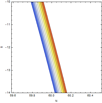
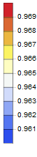
Figure 1: Scalar spectral index as a function of $\delta$ and e-folds $N$. As shown, the area of viability is quite slim for these set of values. It should also be stated that $\lambda$ needs to be fine tuned such that $n_{\mathcal{S}}$ deviates from unity.

$$\centering\Omega_{gw}(k)=\frac{\Omega_{gw,0}h^{2}}{\Omega_{r,0}h^{2}}\bigg{(}\frac{g_{*}}{g_{0}}\bigg{)}^{\frac{1}{3}}\mathrm{e}^{4N_{pre}}\,,\@add@centering$$ (69)

which in the context of Gauss-Bonnet model, it is mildly affected by the factor $X=\frac{8\kappa^{2}\dot{\xi}H}{\alpha}$. In general, the Gauss-Bonnet scalar coupling function and its dynamical evolution according to Eq. (10) has interesting applications in the energy spectrum of gravitational waves, especially in the high frequency regime and we shall showcase this explicitly in the following section. For the time being, let us examine an inflationary model.

Figure 2: Tensor-to-scalar ratio depending on $N$ and $\delta$. In contrast to the scalar spectral index, the area of viability is quite large and there exist a plethora of values capable of satisfying the condition $r<0.064$.

V.1 The case of $\xi(\phi)=\lambda\tanh(\delta\kappa\phi)\,$

In this explicit example, we shall consider that the Gauss-Bonnet scalar coupling function is known and is specified by the following expression [59],

$$\centering\xi(\phi)=\lambda\tanh(\delta\kappa\phi)\,,\@add@centering$$ (70)

where $\lambda$ and $\delta$ are arbitrary for the time being dimensionless parameters with the first denoting the amplitude of the coupling function. In order to specify the scalar potential, we shall follow the steps mentioned before in the inflationary phenomenology. Firstly, by solving the continuity equation under the slow-roll assumption (21) with respect to the scalar potential, it becomes clear that for the aforementioned Gauss-Bonnet coupling,

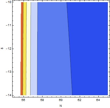
Figure 3: Tensor spectral index $n_{\mathcal{T}}$ versus e-folds and exponent $\delta$. As shown, there exist a lot of values that manage to generate a blue spectrum.

$$\centering V(\phi)=\frac{1}{\Lambda\kappa^{4}\sinh^{-\frac{1}{2\delta^{2}}}(\delta\kappa\phi)-\frac{4}{3}\kappa^{4}\lambda\tanh^{2}(\delta\kappa\phi)^{\frac{1}{2}-\frac{1}{4\delta^{2}}}\coth(\delta\kappa\phi)\text{sech}^{2}(\delta\kappa\phi)^{\frac{1}{4\delta^{2}}}B_{\text{sech}^{2}(\delta\kappa\phi)}\left(1-\frac{1}{4\delta^{2}},\frac{1}{4}\left(2+\frac{1}{\delta^{2}}\right)\right)}\,,\@add@centering$$ (71)

where $\Lambda$ is the integration parameter and $B_{\text{sech}}$ is the incomplete beta function. This is a quite non-trivial potential, however it is completely specified by the free parameters of the model. Note that hereafter for simplicity it is assumed that $\alpha=1$. In consequence, since the inflationary dynamics is mainly specified by the ratio $\frac{\xi^{\prime}}{\xi^{\prime\prime}}=-\frac{\coth(\delta\kappa\phi)}{2\delta\kappa}$, one can extract information about the scalar field. In particular, with regards to the free parameters of the model, the initial and final value of the scalar field during inflation reads,

$$\centering\phi_{k}=\frac{1}{\delta\kappa}\cosh^{-1}\left(\frac{e^{N/2}}{\sqrt{1-\frac{1}{8\delta^{2}}}}\right)\,,\@add@centering$$ (72)

$$\centering\phi_{end}=-\frac{\coth^{-1}\left(2\sqrt{2}\delta\right)}{\delta\kappa}\,.\@add@centering$$ (73)

Let us see how the model could yield viable results. Assuming that $(N,\delta,\lambda,\Lambda)=(60,-12,-10^{33},3\times 10^{9})$, it can easily be inferred that $n_{\mathcal{S}}=0.966794$, $r=0.0138885$ and $n_{\mathcal{T}}=0.0025591$ which are in agreement with observations [163], see Figs. 1, 2, 3 and see also Fig. 4 for a more detailed analysis where the resulting phenomenology is confronted with the latest Planck likelihood curves.

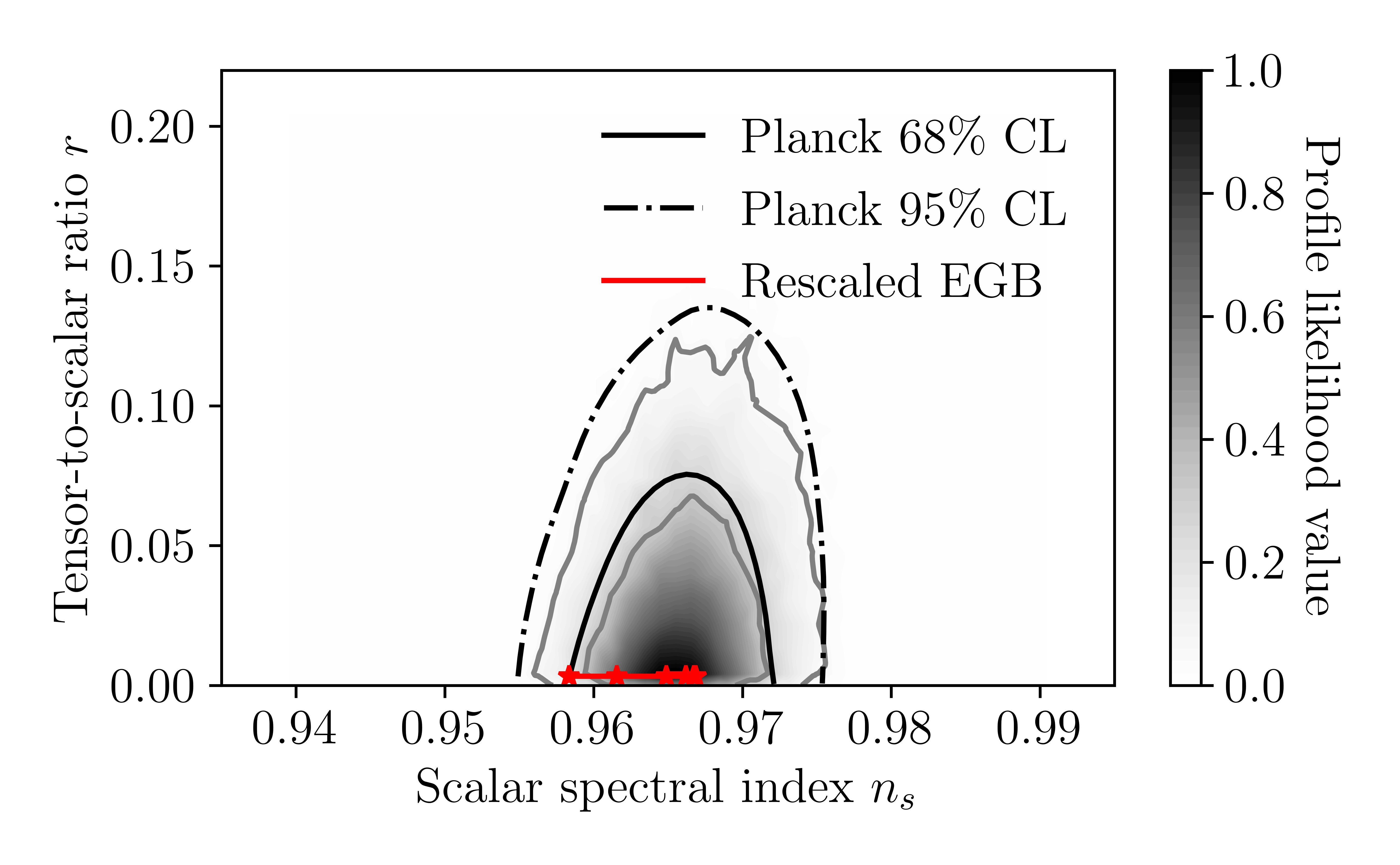
Figure 4: The phenomenological confrontation of the model $\xi(\phi)=\lambda\tanh(\delta\kappa\phi)\,$ with the latest Planck likelihood curves.

It is interesting to mention that the tensor spectral index is positive due to the fact that $\beta(\phi_{k})=2.47491$ is greater than unity and as it was proposed in the previous sections it is also worth stating that the Swampland criteria are met since $-\frac{V^{\prime\prime}(\phi_{k})}{\kappa^{2}V(\phi_{k})}=2.43902>\mathcal{O}(1)$. For this model, one finds that $\phi_{k}=-2.5578M_{Pl}$ while $\phi_{end}=-0.002456M_{Pl}$ which states that the scalar field reaches zero as time flows by. The form of the scalar potential is shown in Fig. 5. Furthermore, the slow-roll conditions are met since $\epsilon_{1}=0.000868=-\epsilon_{2}$, $\epsilon_{3}=0.01572$ and $\epsilon_{4}=-0.00215$.

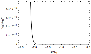
Figure 5: Diagrammatic representation of the scalar potential. An shown, negative values for the scalar field result in an apparent increase of the strength of the potential while the limit $V\to 0$ is reached for $\phi=0$ which serves as the minimum value.

Now in order to study subsequent cosmological eras, the value for $X_{end}$ is required. This can be derived from the very definition of $X=\frac{8\kappa^{2}\dot{\xi}H}{\alpha}$ at the end of inflation where $\dot{\phi}_{end}^{2}=V_{end}$. In the end, one finds that,

$$\centering X_{end}=\pm\frac{4\sqrt{2}\kappa^{3}V_{end}\xi^{\prime}_{end}}{\alpha^{\frac{3}{2}}\sqrt{1-X_{end}}}\,,\@add@centering$$ (74)

which can be solved numerically for the same set of parameters that were used in the inflationary phenomenology. Note that a viable approach requires $X_{end}<1$, however there exists no limit if $X<0$. Afterwards, by specifying $T_{re}$, $\omega_{pre}$ and substituting $\zeta$, information about the preheating and preheating era can be extracted. This is shown in Figs. 6 and Fig. 7 respectively, where as shown, while the duration of preheating increases with $\omega_{pre}$, the duration of the reheating era decreases. For a typical example, consider the case of $\zeta=10^{3}$ with $\omega_{pre}=\frac{1}{5}$ and $T_{re}=10^{8}$GeV where it turns out that $N_{pre}\simeq 11.6$ and $N_{re}\simeq 0.81$.

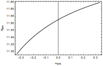
Figure 6: Duration of preheating $N_{pre}$ as a function of the preheating EoS. It becomes clear that the duration increases with the increase of $\omega_{pre}$. For this numerical analysis, it is assumed that $T_{re}=10^{8}$GeV and $\zeta=10^{3}$.

VI Amplification of the energy spectrum of primordial gravitational waves

Finally, in this section we shall briefly discuss the impact that modifications in Einstein’s gravity have on the energy spectrum of gravitational waves. In order to extract information about the impact that the Gauss-Bonnet scalar coupling function has on the overall phenomenology, one needs to study the behavior of tensor perturbations. Suppose that the perturbed metric now reads,

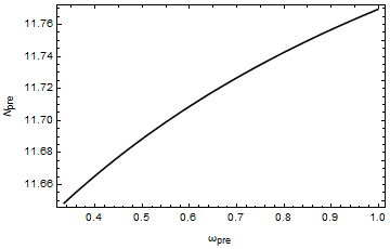
Figure 7: Reheating duration for the same set of parameters. In contrast to $N_{pre}$, $N_{re}$ seems to decrease with the increase of the $\omega_{pre}$.

$$\centering ds^{2}=-dt^{2}+a^{2}(t)(\delta_{ij}+h_{ij}(t,\bm{x}))dx^{i}dx^{j}\,,\@add@centering$$ (75)

where $h_{ij}(t,\bm{x})$ describes tensor perturbations in configuration space. For consistency, tensor perturbations need to be traceless and transverse therefore the conditions $\delta^{ij}h_{ij}=0=\partial_{i}h^{ij}$ must be respected. In consequence, by varying the perturbed action, the Fourier transformation of tensor modes must satisfy the following equation,

$$\centering\ddot{h}(k)+(3+a_{M})H\dot{h}(k)+\frac{k^{2}}{a^{2}}h(k)=0\,,\@add@centering$$ (76)

where $a_{M}=\frac{\dot{Q}_{t}}{HQ_{t}}$ denotes the running of the Planck mass [127, 151]. Note that the Gauss-Bonnet model is a subclass of Horndeski’s theory that affects the Planck mass therefore tensor modes are subsequently affected. This was showcased previously when the tensor spectral index was presented. Usually, for GR, $a_{M}=0$ therefore the solution is known. Due to the presence of the running Planck mass, one needs to extract a new solution for Eq. (76). This can be achieved by making use of the WKB approximation [127] where the solution is connected to the GR result as shown below,

$$\centering h=\mathrm{e}^{-\mathcal{D}}h_{GR}\,,\@add@centering$$ (77)

where $h_{ij}=he_{ij}$ and $\mathcal{D}=\int_{0}^{z}dz^{\prime}\frac{a_{M}}{1+z^{\prime}}$. This in turn implies that modified theories of gravity which predict a nontrivial running for the Planck mass manage, to affect the energy spectrum of gravitational waves by means of the exponential factor $\mathrm{e}^{-\mathcal{D}}$. This factor can result in an effected dumping or amplification of the energy spectrum. This becomes clear from the definition of the energy spectrum which in this case reads [127],

$$\centering\Omega_{gw}(k)=\frac{1}{\rho_{crit}}\frac{d\bra{0}\rho_{gw}\ket{0}}{d\ln k}=\frac{k^{2}\Delta_{h}^{2}}{12H_{0}^{2}}\,,\@add@centering$$ (78)

where $\Delta_{h}^{2}=\frac{d\bra{0}h_{ij}^{2}\ket{0}}{d\ln k}$ is the tensor power spectrum. In the context of modified theories of gravity, the tensor power spectrum is given by the following expression [128, 129, 130, 131, 132, 133, 134, 135, 136, 137, 138, 139, 140, 141, 142, 143, 144, 145, 146, 147, 60, 148, 149, 150],

$$\centering\Delta_{h}^{2}\@add@centering =\mathrm{e}^{-2\mathcal{D}}\Delta_{h}^{(p)2}\bigg{(}\frac{\Omega_{m}}{\Omega_{\Lambda}}\bigg{)}^{2}\bigg{(}\frac{g_{*}(T_{in})}{g_{*0}}\bigg{)}\bigg{(}\frac{g_{*s0}}{g_{*s}(T_{in})}\bigg{)}^{\frac{4}{3}}\bigg{(}\overline{\frac{3j_{1}(k\tau_{0})}{k\tau_{0}}}\bigg{)}^{2}T_{1}^{2}(x_{eq})T_{2}^{2}(x_{R})\,,$$ (79)

where $g_{*}$ denotes the relativistic degrees of freedom at different cosmological eras, hence the reason why it is a temperature dependent quantity, $T_{i}$ specifies the transfer function at a given era dictates by $x$ witch denotes the ratio of the pivot scale with either the matter-radiation equivalence of the reheating scale and finally, $\Delta_{h}^{(p)2}$ denotes the primordial tensor power spectrum which is connected to the amplitude of tensor perturbations as,

$$\centering\Delta_{h}^{(p)2}=\mathcal{A}_{\mathcal{T}}\bigg{(}\frac{k}{k_{*}}\bigg{)}^{n_{\mathcal{T}}}\,.\@add@centering$$ (80)

At this point, it should be stated that the amplitude of tensor perturbations, in contrast to scalar perturbations, has yet to be observed however it is connected to the tensor-to-scalar ratio as $\mathcal{A}_{\mathcal{T}}=r\mathcal{P}_{\zeta}$. Furthermore, the tensor spectral index that participates in the exponent should be treated as a frequency dependent parameter. In the end, by using Eq. (35) and by combining all the above expressions, one can show that [127],

$$\centering\Omega_{gw}(k)=\mathrm{e}^{-2\mathcal{D}}\frac{k^{2}}{12H_{0}^{2}}r\mathcal{P}_{\zeta}(k_{*})\bigg{(}\frac{k}{k_{*}}\bigg{)}^{n_{\mathcal{T}}(k_{*})+\frac{a_{\mathcal{T}(k_{*})}}{2}\ln\frac{k}{k_{*}}}\bigg{(}\frac{\Omega_{m}}{\Omega_{\Lambda}}\bigg{)}^{2}\bigg{(}\frac{g_{*}(T_{in})}{g_{*0}}\bigg{)}\bigg{(}\frac{g_{*s0}}{g_{*s}(T_{in})}\bigg{)}^{\frac{4}{3}}\bigg{(}\overline{\frac{3j_{1}(k\tau_{0})}{k\tau_{0}}}\bigg{)}^{2}T_{1}^{2}(x_{eq})T_{2}^{2}(x_{R})\,.\@add@centering$$ (81)

At this point, two key features need to be highlighted. Firstly, a negative factor $\mathcal{D}$ can in fact result in an apparent enhancement of the energy spectrum measured today at all frequency ranges. Secondly, provided that a blue-tilted tensor spectral index is produced for $\beta>1$, it becomes clear that modes which become subhorizon in primordial eras right after inflation, result in an additional apparent amplification of the energy spectrum, however this is possible only in the high frequency regime. This is an interesting statement since these modes carry information about subsequent eras such as reheating and radiation domination and by simply studying high frequencies, information about such eras can be obtained. Modified theories of gravity can in principle result in an apparent enhancement or dumping thus making the detection of gravitational waves at these frequencies either an easier or more difficult task.

For the model at hand, the modified Planck mass has already been computed in terms of the auxiliary parameter $Q_{t}=\frac{\alpha}{\kappa^{2}}-8\dot{\xi}H$ denoting the shifted Planck mass squared. In consequence, if one wants to compute the running Planck mass $a_{M}$, provided that the constraint $\ddot{\xi}=H\dot{\xi}$ is imposed, then it can easily be inferred that,

$$\centering a_{M}=-\frac{X}{1-X}\bigg{[}1+\frac{\dot{H}}{H^{2}}\bigg{]}\,,\@add@centering$$ (82)

where $X=\frac{8\kappa^{2}\dot{\xi}H}{\alpha}$. Hence, the deceleration parameter $q=-1-\frac{\dot{H}}{H^{2}}$ appears in the running Planck mass. Now assuming that $1-X>0$, $X<0$, the running Planck mass is negative during deceleration hence the amplitude can in principle be enhanced. In general, by solving Eq. (16) in the presence of perfect matter fluids with respect to $\dot{H}$, the deceleration parameter can be extracted and in consequence, one can show that the running Planck mass can be written with respect to dynamical variables as,

$$\centering a_{M}=\frac{X}{(1-X)^{2}}\bigg{[}-(1-X)+3Y^{2}+\frac{4\Omega_{\alpha r}+3\Omega_{\alpha m}}{2}\bigg{]}\,,\@add@centering$$ (83)

where $Y=\frac{\kappa\dot{\phi}}{\sqrt{6\alpha}H}$ and $\Omega_{\alpha i}=\frac{\kappa^{2}\rho_{i}}{3\alpha H^{2}}$. Generally speaking, for $\alpha\to 1$ the usual description emerges however under the assumption that $\alpha$ is an effective rescaled version of the Einstein-Hilbert action due to the fact that higher order curvature corrections provided by an $f(R)$ gravity result in an effective shift of the coefficient of the Ricci scalar primordially, one can extract information about the deceleration parameter by studying $z=\frac{R}{6H^{2}}$ and in this approach,

$$\centering a_{M}=\frac{X}{1-X}(1-z)\,.\@add@centering$$ (84)

As it proves however, the amplification caused by the extra $a_{M}$ contribution on the energy spectrum of the primordial gravitational waves is insignificant and of the order unity for many rescaled Einstein-Gauss-Bonnet models we examined, this is also common for ordinary Einstein-Gauss-Bonnet model [60]. Thus the amplification of the primordial gravitational waves energy spectrum can only occur due to a significantly large and blue tilted tensor spectral index.

VII Conclusions

In the present article the inflationary dynamics of the Einstein-Gauss-Bonnet theory for an arbitrary Gauss-Bonnet scalar coupling functions was considered. It was shown that under the assumption that tensor perturbations propagate through spacetime with the velocity of light, therefore predicting primordial massless gravitons and also being in agreement with the GW170817 event, the degrees of freedom still remain exactly the same as in the case of a canonical scalar field. Afterwards, the spectral indices and the tensor-to-scalar ratio were derived by making use of several auxiliary dimensionless indices and as shown the numerical value of the observables is completely dictated by three parameters of the model, namely the first slow-roll index $\epsilon_{1}$ which quantifies inflation, and parameters $\beta$ and $\gamma$ that carry information about the properties of the Gauss-Bonnet scalar coupling function. In turn, the free parameters of a given model should completely specify the above three parameters. Afterwards the running of the spectral indices was considered briefly were it was shown that regardless of the fact that a constrained Einstein-Gauss-Bonnet model was studied, which states that a handful of parameters may not necessarily be small (compatible with a slow-roll evolution) during the first horizon crossing, due to the fact that $\ddot{\xi}=H\dot{\xi}$, the value of the first derivatives $a_{\mathcal{S}/\mathcal{T}}(k_{*})$ evaluated at the pivot scale seems to be in agreement with observations. Finally, the Swampland criteria were briefly examined, were it was shown that while the second and third criterion scale as $\sqrt{\epsilon_{1}}$ and $\epsilon_{1}$ respectively, it is possible to become simultaneously greater than unity if a small rescaling parameter is used. In addition, having $\beta>1$ seems to satisfy the third criterion while a blue-tilted tensor spectral index is obtained. Also it was proved that the tracking condition can be satisfied in the constrained Gauss-Bonnet model only if the Swampland criteria are met simultaneously, however a blue-tilted tensor spectral index cannot be derived in that case. In addition, the model $\xi\sim 1/V$, along with $\xi\sim V$, were excluded from the tracking condition since the first is possible only for power-law model with an exponent lesser than unity while the latter is possible for exponential scalar functions which cannot describe the inflationary era properly in the constrained Gauss-Bonnet formalism. Afterwards the preheating era was briefly discussed where the duration $N_{pre}$ was derived as a function of the duration of the reheating era and temperature as well as the effective EoS. Assuming that the propagation velocity of tensor perturbations is fixed to coincide with the speed of light, it was shown that the energy density at the end of inflation is shifted by a factor of $1/1-X$ where $X=\frac{8\kappa^{2}\dot{\xi}H}{\alpha}$. The model was also tested by assuming that the Gauss-Bonnet scalar coupling function has a hyperbolic form $\xi(\phi)=\lambda\tanh(\delta\kappa\phi)$ where it was shown that the model can indeed be in agreement with observations. In consequence, a brief comment on the energy spectrum of primordial gravitational waves was made and as shown, the energy spectrum in the constrained Gauss-Bonnet model can be enhanced by either a negative factor $\mathcal{D}$ or by a positive value of the tensor spectral index, or in other words for $\beta>1$. The latter case is connected to the amplification of the energy spectrum of primordial gravitational waves in the high frequency region, in which modes re-enter the horizon relatively fast and can thus shine light towards primordial cosmological eras of interest. From a theoretical perspective, it would be interesting to see how certain inflationary models can yield viable results under the assumption that $\ddot{\xi}=H\dot{\xi}$ and also whether the Swampland criteria, if satisfied, are in agreement with the tracking condition. Furthermore, the possibility of a kinetic coupling of the form $\frac{1}{2}\xi(\phi)G^{\mu\nu}\nabla_{\mu}\phi\nabla_{\nu}\phi$ in the gravitational action may be promising since the constraint on the propagation velocity of tensor perturbations is now altered. We aim to address these interesting topics, along with a complete study of the rescaled Einstein-Gauss-Bonnet theories phenomenology, in future works.

References

- [1] A. D. Linde, Lect. Notes Phys. 738 (2008) 1 [arXiv:0705.0164 [hep-th]].
- [2] D. S. Gorbunov and V. A. Rubakov, “Introduction to the theory of the early universe: Cosmological perturbations and inflationary theory,” Hackensack, USA: World Scientific (2011) 489 p;
- [3] A. Linde, arXiv:1402.0526 [hep-th];
- [4] D. H. Lyth and A. Riotto, Phys. Rept. 314 (1999) 1 [hep-ph/9807278].
- [5] J. Baker, J. Bellovary, P. L. Bender, E. Berti, R. Caldwell, J. Camp, J. W. Conklin, N. Cornish, C. Cutler and R. DeRosa, et al. [arXiv:1907.06482 [astro-ph.IM]].
- [6] T. L. Smith and R. Caldwell, Phys. Rev. D 100 (2019) no.10, 104055 doi:10.1103/PhysRevD.100.104055 [arXiv:1908.00546 [astro-ph.CO]].
- [7] J. Crowder and N. J. Cornish, Phys. Rev. D 72 (2005), 083005 doi:10.1103/PhysRevD.72.083005 [arXiv:gr-qc/0506015 [gr-qc]].
- [8] T. L. Smith and R. Caldwell, Phys. Rev. D 95 (2017) no.4, 044036 doi:10.1103/PhysRevD.95.044036 [arXiv:1609.05901 [gr-qc]].
- [9] N. Seto, S. Kawamura and T. Nakamura, Phys. Rev. Lett. 87 (2001), 221103 doi:10.1103/PhysRevLett.87.221103 [arXiv:astro-ph/0108011 [astro-ph]].
- [10] S. Kawamura, M. Ando, N. Seto, S. Sato, M. Musha, I. Kawano, J. Yokoyama, T. Tanaka, K. Ioka and T. Akutsu, et al. [arXiv:2006.13545 [gr-qc]].
- [11] K. N. Abazajian et al. [CMB-S4], [arXiv:1610.02743 [astro-ph.CO]].
- [12] M. H. Abitbol et al. [Simons Observatory], Bull. Am. Astron. Soc. 51 (2019), 147 [arXiv:1907.08284 [astro-ph.IM]].
- [13] J. c. Hwang and H. Noh, Phys. Rev. D 71 (2005) 063536 doi:10.1103/PhysRevD.71.063536 [gr-qc/0412126].
- [14] S. Nojiri, S. D. Odintsov and M. Sami, Phys. Rev. D 74 (2006) 046004 doi:10.1103/PhysRevD.74.046004 [hep-th/0605039].
- [15] G. Cognola, E. Elizalde, S. Nojiri, S. Odintsov and S. Zerbini, Phys. Rev. D 75 (2007) 086002 doi:10.1103/PhysRevD.75.086002 [hep-th/0611198].
- [16] S. Nojiri, S. D. Odintsov and M. Sasaki, Phys. Rev. D 71 (2005) 123509 doi:10.1103/PhysRevD.71.123509 [hep-th/0504052].
- [17] S. Nojiri and S. D. Odintsov, Phys. Lett. B 631 (2005) 1 doi:10.1016/j.physletb.2005.10.010 [hep-th/0508049].
- [18] M. Satoh, S. Kanno and J. Soda, Phys. Rev. D 77 (2008) 023526 doi:10.1103/PhysRevD.77.023526 [arXiv:0706.3585 [astro-ph]].
- [19] K. Bamba, A. N. Makarenko, A. N. Myagky and S. D. Odintsov, JCAP 1504 (2015) 001 doi:10.1088/1475-7516/2015/04/001 [arXiv:1411.3852 [hep-th]].
- [20] Z. Yi, Y. Gong and M. Sabir, Phys. Rev. D 98 (2018) no.8, 083521 doi:10.1103/PhysRevD.98.083521 [arXiv:1804.09116 [gr-qc]].
- [21] Z. K. Guo and D. J. Schwarz, Phys. Rev. D 80 (2009) 063523 doi:10.1103/PhysRevD.80.063523 [arXiv:0907.0427 [hep-th]].
- [22] Z. K. Guo and D. J. Schwarz, Phys. Rev. D 81 (2010) 123520 doi:10.1103/PhysRevD.81.123520 [arXiv:1001.1897 [hep-th]].
- [23] P. X. Jiang, J. W. Hu and Z. K. Guo, Phys. Rev. D 88 (2013) 123508 doi:10.1103/PhysRevD.88.123508 [arXiv:1310.5579 [hep-th]].
- [24] P. Kanti, R. Gannouji and N. Dadhich, Phys. Rev. D 92 (2015) no.4, 041302 doi:10.1103/PhysRevD.92.041302 [arXiv:1503.01579 [hep-th]].
- [25] C. van de Bruck, K. Dimopoulos, C. Longden and C. Owen, arXiv:1707.06839 [astro-ph.CO].
- [26] P. Kanti, J. Rizos and K. Tamvakis, Phys. Rev. D 59 (1999) 083512 doi:10.1103/PhysRevD.59.083512 [gr-qc/9806085].
- [27] E. O. Pozdeeva, M. R. Gangopadhyay, M. Sami, A. V. Toporensky and S. Y. Vernov, Phys. Rev. D 102 (2020) no.4, 043525 doi:10.1103/PhysRevD.102.043525 [arXiv:2006.08027 [gr-qc]].
- [28] S. Vernov and E. Pozdeeva, Universe 7 (2021) no.5, 149 doi:10.3390/universe7050149 [arXiv:2104.11111 [gr-qc]].
- [29] E. O. Pozdeeva and S. Y. Vernov, Eur. Phys. J. C 81 (2021) no.7, 633 doi:10.1140/epjc/s10052-021-09435-8 [arXiv:2104.04995 [gr-qc]].
- [30] S. Koh, B. H. Lee, W. Lee and G. Tumurtushaa, Phys. Rev. D 90 (2014) no.6, 063527 doi:10.1103/PhysRevD.90.063527 [arXiv:1404.6096 [gr-qc]].
- [31] B. Bayarsaikhan, S. Koh, E. Tsedenbaljir and G. Tumurtushaa, JCAP 11 (2020), 057 doi:10.1088/1475-7516/2020/11/057 [arXiv:2005.11171 [gr-qc]].
- [32] G. Tumurtushaa, S. Koh and B. H. Lee, PoS ICHEP2018 (2019), 090 doi:10.22323/1.340.0090
- [33] I. Fomin, Eur. Phys. J. C 80 (2020) no.12, 1145 doi:10.1140/epjc/s10052-020-08718-w [arXiv:2004.08065 [gr-qc]].
- [34] M. De Laurentis, M. Paolella and S. Capozziello, Phys. Rev. D 91 (2015) no.8, 083531 doi:10.1103/PhysRevD.91.083531 [arXiv:1503.04659 [gr-qc]].
-
[35]
Scalar Field Cosmology, S. Chervon, I. Fomin, V. Yurov and
A. Yurov, World Scientific 2019,
doi:10.1142/11405 - [36] K. Nozari and N. Rashidi, Phys. Rev. D 95 (2017) no.12, 123518 doi:10.1103/PhysRevD.95.123518 [arXiv:1705.02617 [astro-ph.CO]].
- [37] S. D. Odintsov and V. K. Oikonomou, Phys. Rev. D 98 (2018) no.4, 044039 doi:10.1103/PhysRevD.98.044039 [arXiv:1808.05045 [gr-qc]].
- [38] S. Kawai, M. a. Sakagami and J. Soda, Phys. Lett. B 437, 284 (1998) doi:10.1016/S0370-2693(98)00925-3 [gr-qc/9802033].
- [39] Z. Yi and Y. Gong, Universe 5 (2019) no.9, 200 doi:10.3390/universe5090200 [arXiv:1811.01625 [gr-qc]].
- [40] C. van de Bruck, K. Dimopoulos and C. Longden, Phys. Rev. D 94 (2016) no.2, 023506 doi:10.1103/PhysRevD.94.023506 [arXiv:1605.06350 [astro-ph.CO]].
- [41] B. Kleihaus, J. Kunz and P. Kanti, Phys. Lett. B 804 (2020), 135401 doi:10.1016/j.physletb.2020.135401 [arXiv:1910.02121 [gr-qc]].
- [42] A. Bakopoulos, P. Kanti and N. Pappas, Phys. Rev. D 101 (2020) no.4, 044026 doi:10.1103/PhysRevD.101.044026 [arXiv:1910.14637 [hep-th]].
- [43] K. i. Maeda, N. Ohta and R. Wakebe, Eur. Phys. J. C 72 (2012) 1949 doi:10.1140/epjc/s10052-012-1949-6 [arXiv:1111.3251 [hep-th]].
- [44] A. Bakopoulos, P. Kanti and N. Pappas, Phys. Rev. D 101 (2020) no.8, 084059 doi:10.1103/PhysRevD.101.084059 [arXiv:2003.02473 [hep-th]].
- [45] W. Y. Ai, Commun. Theor. Phys. 72 (2020) no.9, 095402 doi:10.1088/1572-9494/aba242 [arXiv:2004.02858 [gr-qc]].
- [46] V. K. Oikonomou and F. P. Fronimos, EPL 131 (2020) no.3, 30001 doi:10.1209/0295-5075/131/30001 [arXiv:2007.11915 [gr-qc]].
- [47] S. D. Odintsov, V. K. Oikonomou and F. P. Fronimos, Annals Phys. 420 (2020), 168250 doi:10.1016/j.aop.2020.168250 [arXiv:2007.02309 [gr-qc]].
- [48] V. K. Oikonomou and F. P. Fronimos, Class. Quant. Grav. 38 (2021) no.3, 035013 doi:10.1088/1361-6382/abce47 [arXiv:2006.05512 [gr-qc]].
- [49] S. D. Odintsov and V. K. Oikonomou, Phys. Lett. B 805 (2020), 135437 doi:10.1016/j.physletb.2020.135437 [arXiv:2004.00479 [gr-qc]].
- [50] S. D. Odintsov, V. K. Oikonomou, F. P. Fronimos and S. A. Venikoudis, Phys. Dark Univ. 30 (2020), 100718 doi:10.1016/j.dark.2020.100718 [arXiv:2009.06113 [gr-qc]].
- [51] S. A. Venikoudis and F. P. Fronimos, Eur. Phys. J. Plus 136 (2021) no.3, 308 doi:10.1140/epjp/s13360-021-01298-y [arXiv:2103.01875 [gr-qc]].
- [52] S. B. Kong, H. Abdusattar, Y. Yin and Y. P. Hu, [arXiv:2108.09411 [gr-qc]].
- [53] R. Easther and K. i. Maeda, Phys. Rev. D 54 (1996) 7252 doi:10.1103/PhysRevD.54.7252 [hep-th/9605173].
- [54] I. Antoniadis, J. Rizos and K. Tamvakis, Nucl. Phys. B 415 (1994) 497 doi:10.1016/0550-3213(94)90120-1 [hep-th/9305025].
- [55] I. Antoniadis, C. Bachas, J. R. Ellis and D. V. Nanopoulos, Phys. Lett. B 257 (1991), 278-284 doi:10.1016/0370-2693(91)91893-Z
- [56] P. Kanti, N. Mavromatos, J. Rizos, K. Tamvakis and E. Winstanley, Phys. Rev. D 54 (1996), 5049-5058 doi:10.1103/PhysRevD.54.5049 [arXiv:hep-th/9511071 [hep-th]].
- [57] P. Kanti, N. Mavromatos, J. Rizos, K. Tamvakis and E. Winstanley, Phys. Rev. D 57 (1998), 6255-6264 doi:10.1103/PhysRevD.57.6255 [arXiv:hep-th/9703192 [hep-th]].
- [58] D. A. Easson, T. Manton and A. Svesko, JCAP 10 (2020), 026 doi:10.1088/1475-7516/2020/10/026 [arXiv:2005.12292 [hep-th]].
- [59] N. Rashidi and K. Nozari, Astrophys. J. 890, 58 doi:10.3847/1538-4357/ab6a10 [arXiv:2001.07012 [astro-ph.CO]].
- [60] V. K. Oikonomou, Astropart. Phys. 141 (2022), 102718 doi:10.1016/j.astropartphys.2022.102718 [arXiv:2204.06304 [gr-qc]].
- [61] B. P. Abbott et al. [LIGO Scientific and Virgo], Phys. Rev. Lett. 119 (2017) no.16, 161101 doi:10.1103/PhysRevLett.119.161101 [arXiv:1710.05832 [gr-qc]].
- [62] B. P. Abbott et al. [LIGO Scientific, Virgo, Fermi-GBM and INTEGRAL], Astrophys. J. Lett. 848 (2017) no.2, L13 doi:10.3847/2041-8213/aa920c [arXiv:1710.05834 [astro-ph.HE]].
- [63] B. P. Abbott et al. “Multi-messenger Observations of a Binary Neutron Star Merger,” Astrophys. J. 848 (2017) no.2, L12 doi:10.3847/2041-8213/aa91c9 [arXiv:1710.05833 [astro-ph.HE]].
- [64] J. M. Ezquiaga and M. Zumalacárregui, Phys. Rev. Lett. 119 (2017) no.25, 251304 doi:10.1103/PhysRevLett.119.251304 [arXiv:1710.05901 [astro-ph.CO]].
- [65] T. Baker, E. Bellini, P. G. Ferreira, M. Lagos, J. Noller and I. Sawicki, Phys. Rev. Lett. 119 (2017) no.25, 251301 doi:10.1103/PhysRevLett.119.251301 [arXiv:1710.06394 [astro-ph.CO]].
- [66] P. Creminelli and F. Vernizzi, Phys. Rev. Lett. 119 (2017) no.25, 251302 doi:10.1103/PhysRevLett.119.251302 [arXiv:1710.05877 [astro-ph.CO]].
- [67] J. Sakstein and B. Jain, Phys. Rev. Lett. 119 (2017) no.25, 251303 doi:10.1103/PhysRevLett.119.251303 [arXiv:1710.05893 [astro-ph.CO]].
- [68] S. D. Odintsov, V. K. Oikonomou and F. P. Fronimos, Nucl. Phys. B 958 (2020), 115135 doi:10.1016/j.nuclphysb.2020.115135 [arXiv:2003.13724 [gr-qc]].
- [69] V. K. Oikonomou, Class. Quant. Grav. 38 (2021) no.19, 195025 doi:10.1088/1361-6382/ac2168 [arXiv:2108.10460 [gr-qc]].
- [70] V. K. Oikonomou, P. D. Katzanis and I. C. Papadimitriou, Class. Quant. Grav. 39 (2022) no.9, 095008 doi:10.1088/1361-6382/ac5eba [arXiv:2203.09867 [gr-qc]].
- [71] C. Vafa, [arXiv:hep-th/0509212 [hep-th]].
- [72] H. Ooguri and C. Vafa, Nucl. Phys. B 766 (2007) 21 doi:10.1016/j.nuclphysb.2006.10.033 [hep-th/0605264].
- [73] E. Palti, C. Vafa and T. Weigand, arXiv:2003.10452 [hep-th].
- [74] R. Brandenberger, V. Kamali and R. O. Ramos, arXiv:2002.04925 [hep-th].
- [75] R. Blumenhagen, M. Brinkmann and A. Makridou, JHEP 2002 (2020) 064 [JHEP 2020 (2020) 064] doi:10.1007/JHEP02(2020)064 [arXiv:1910.10185 [hep-th]].
- [76] Z. Wang, R. Brandenberger and L. Heisenberg, arXiv:1907.08943 [hep-th].
- [77] M. Benetti, S. Capozziello and L. L. Graef, Phys. Rev. D 100 (2019) no.8, 084013 doi:10.1103/PhysRevD.100.084013 [arXiv:1905.05654 [gr-qc]].
- [78] E. Palti, Fortsch. Phys. 67 (2019) no.6, 1900037 doi:10.1002/prop.201900037 [arXiv:1903.06239 [hep-th]].
- [79] R. G. Cai, S. Khimphun, B. H. Lee, S. Sun, G. Tumurtushaa and Y. L. Zhang, Phys. Dark Univ. 26 (2019) 100387 doi:10.1016/j.dark.2019.100387 [arXiv:1812.11105 [hep-th]].
- [80] Y. Akrami, R. Kallosh, A. Linde and V. Vardanyan, Fortsch. Phys. 67 (2019) no.1-2, 1800075 doi:10.1002/prop.201800075 [arXiv:1808.09440 [hep-th]].
- [81] S. Mizuno, S. Mukohyama, S. Pi and Y. L. Zhang, JCAP 1909 (2019) no.09, 072 doi:10.1088/1475-7516/2019/09/072 [arXiv:1905.10950 [hep-th]].
- [82] V. Aragam, S. Paban and R. Rosati, arXiv:1905.07495 [hep-th].
- [83] S. Brahma and M. W. Hossain, Phys. Rev. D 100 (2019) no.8, 086017 doi:10.1103/PhysRevD.100.086017 [arXiv:1904.05810 [hep-th]].
- [84] U. Mukhopadhyay and D. Majumdar, Phys. Rev. D 100 (2019) no.2, 024006 doi:10.1103/PhysRevD.100.024006 [arXiv:1904.01455 [gr-qc]].
- [85] S. Brahma and M. W. Hossain, JHEP 1906 (2019) 070 doi:10.1007/JHEP06(2019)070 [arXiv:1902.11014 [hep-th]].
- [86] M. R. Haque and D. Maity, Phys. Rev. D 99 (2019) no.10, 103534 doi:10.1103/PhysRevD.99.103534 [arXiv:1902.09491 [hep-th]].
- [87] J. J. Heckman, C. Lawrie, L. Lin, J. Sakstein and G. Zoccarato, Fortsch. Phys. 67 (2019) no.11, 1900071 doi:10.1002/prop.201900071 [arXiv:1901.10489 [hep-th]].
- [88] B. S. Acharya, A. Maharana and F. Muia, JHEP 1903 (2019) 048 doi:10.1007/JHEP03(2019)048 [arXiv:1811.10633 [hep-th]].
- [89] E. Elizalde and M. Khurshudyan, Phys. Rev. D 99 (2019) no.10, 103533 doi:10.1103/PhysRevD.99.103533 [arXiv:1811.03861 [astro-ph.CO]].
- [90] D. Y. Cheong, S. M. Lee and S. C. Park, Phys. Lett. B 789 (2019) 336 doi:10.1016/j.physletb.2018.12.046 [arXiv:1811.03622 [hep-ph]].
- [91] J. J. Heckman, C. Lawrie, L. Lin and G. Zoccarato, Fortsch. Phys. 67 (2019) no.10, 1900057 doi:10.1002/prop.201900057 [arXiv:1811.01959 [hep-th]].
- [92] W. H. Kinney, S. Vagnozzi and L. Visinelli, Class. Quant. Grav. 36 (2019) no.11, 117001 doi:10.1088/1361-6382/ab1d87 [arXiv:1808.06424 [astro-ph.CO]].
- [93] S. K. Garg and C. Krishnan, JHEP 1911 (2019) 075 doi:10.1007/JHEP11(2019)075 [arXiv:1807.05193 [hep-th]].
- [94] C. M. Lin, Phys. Rev. D 99 (2019) no.2, 023519 doi:10.1103/PhysRevD.99.023519 [arXiv:1810.11992 [astro-ph.CO]].
- [95] S. C. Park, JCAP 1901 (2019) 053 doi:10.1088/1475-7516/2019/01/053 [arXiv:1810.11279 [hep-ph]].
- [96] Y. Olguin-Trejo, S. L. Parameswaran, G. Tasinato and I. Zavala, JCAP 1901 (2019) 031 doi:10.1088/1475-7516/2019/01/031 [arXiv:1810.08634 [hep-th]].
- [97] H. Fukuda, R. Saito, S. Shirai and M. Yamazaki, Phys. Rev. D 99 (2019) no.8, 083520 doi:10.1103/PhysRevD.99.083520 [arXiv:1810.06532 [hep-th]].
- [98] S. J. Wang, Phys. Rev. D 99 (2019) no.2, 023529 doi:10.1103/PhysRevD.99.023529 [arXiv:1810.06445 [hep-th]].
- [99] H. Ooguri, E. Palti, G. Shiu and C. Vafa, Phys. Lett. B 788 (2019) 180 doi:10.1016/j.physletb.2018.11.018 [arXiv:1810.05506 [hep-th]].
- [100] H. Matsui, F. Takahashi and M. Yamada, Phys. Lett. B 789 (2019) 387 doi:10.1016/j.physletb.2018.12.055 [arXiv:1809.07286 [astro-ph.CO]].
- [101] G. Obied, H. Ooguri, L. Spodyneiko and C. Vafa, arXiv:1806.08362 [hep-th].
- [102] P. Agrawal, G. Obied, P. J. Steinhardt and C. Vafa, Phys. Lett. B 784 (2018) 271 doi:10.1016/j.physletb.2018.07.040 [arXiv:1806.09718 [hep-th]].
- [103] H. Murayama, M. Yamazaki and T. T. Yanagida, JHEP 1812 (2018) 032 doi:10.1007/JHEP12(2018)032 [arXiv:1809.00478 [hep-th]].
- [104] M. C. David Marsh, Phys. Lett. B 789 (2019) 639 doi:10.1016/j.physletb.2018.11.001 [arXiv:1809.00726 [hep-th]].
- [105] S. D. Storm and R. J. Scherrer, Phys. Rev. D 102 (2020) no.6, 063519 doi:10.1103/PhysRevD.102.063519 [arXiv:2008.05465 [hep-th]].
- [106] O. Trivedi, [arXiv:2008.05474 [hep-th]].
- [107] U. K. Sharma, [arXiv:2005.03979 [physics.gen-ph]].
- [108] A. Mohammadi, T. Golanbari, J. Enayati, S. Jalalzadeh and K. Saaidi, [arXiv:2011.13957 [gr-qc]].
- [109] O. Trivedi, [arXiv:2011.14316 [astro-ph.CO]].
- [110] C. Han, S. Pi and M. Sasaki, Phys. Lett. B 791 (2019), 314-318 doi:10.1016/j.physletb.2019.02.037 [arXiv:1809.05507 [hep-ph]].
- [111] A. Achúcarro and G. A. Palma, JCAP 02 (2019), 041 doi:10.1088/1475-7516/2019/02/041 [arXiv:1807.04390 [hep-th]].
- [112] Y. Akrami, M. Sasaki, A. R. Solomon and V. Vardanyan, [arXiv:2008.13660 [astro-ph.CO]].
- [113] E. Ó Colgáin, M. H. P. M. van Putten and H. Yavartanoo, Phys. Lett. B 793 (2019), 126-129 doi:10.1016/j.physletb.2019.04.032 [arXiv:1807.07451 [hep-th]].
- [114] E. Ó. Colgáin and H. Yavartanoo, Phys. Lett. B 797 (2019), 134907 doi:10.1016/j.physletb.2019.134907 [arXiv:1905.02555 [astro-ph.CO]].
- [115] A. Banerjee, H. Cai, L. Heisenberg, E. Ó. Colgáin, M. M. Sheikh-Jabbari and T. Yang, [arXiv:2006.00244 [astro-ph.CO]].
- [116] V. K. Oikonomou, I. Giannakoudi, A. Gitsis and K. R. Revis, Int. J. Mod. Phys. D 31 (2022) no.02, 2250001 doi:10.1142/S0218271822500018 [arXiv:2105.11935 [gr-qc]].
- [117] A. Gitsis, K. R. Revis, S. A. Venikoudis and F. P. Fronimos, [arXiv:2301.08126 [gr-qc]].
- [118] S. A. Venikoudis and F. P. Fronimos, Nucl. Phys. B 984 (2022), 115945 doi:10.1016/j.nuclphysb.2022.115945 [arXiv:2208.08333 [gr-qc]].
- [119] K. El Bourakadi, [arXiv:2104.10552 [gr-qc]].
- [120] K. El Bourakadi, M. Ferricha-Alami, H. Filali, Z. Sakhi and M. Bennai, Eur. Phys. J. C 81 (2021) no.12, 1144 doi:10.1140/epjc/s10052-021-09946-4 [arXiv:2209.08581 [gr-qc]].
- [121] S. Koh, B. H. Lee and G. Tumurtushaa, Phys. Rev. D 98 (2018) no.10, 103511 doi:10.1103/PhysRevD.98.103511 [arXiv:1807.04424 [astro-ph.CO]].
- [122] J. L. Cook, E. Dimastrogiovanni, D. A. Easson and L. M. Krauss, JCAP 04 (2015), 047 doi:10.1088/1475-7516/2015/04/047 [arXiv:1502.04673 [astro-ph.CO]].
- [123] K. El Bourakadi, Z. Sakhi and M. Bennai, Int. J. Mod. Phys. A 37 (2022) no.17, 2250117 doi:10.1142/S0217751X22501172 [arXiv:2209.09241 [gr-qc]].
- [124] A. Mazumdar and B. Zaldivar, Nucl. Phys. B 886 (2014), 312-327 doi:10.1016/j.nuclphysb.2014.07.001 [arXiv:1310.5143 [hep-ph]].
- [125] J. Ellis, M. A. G. Garcia, D. V. Nanopoulos and K. A. Olive, JCAP 07 (2015), 050 doi:10.1088/1475-7516/2015/07/050 [arXiv:1505.06986 [hep-ph]].
- [126] T. Hasegawa, N. Hiroshima, K. Kohri, R. S. L. Hansen, T. Tram and S. Hannestad, JCAP 12 (2019), 012 doi:10.1088/1475-7516/2019/12/012 [arXiv:1908.10189 [hep-ph]].
- [127] S. D. Odintsov, V. K. Oikonomou and F. P. Fronimos, Phys. Dark Univ. 35 (2022), 100950 doi:10.1016/j.dark.2022.100950 [arXiv:2108.11231 [gr-qc]].
- [128] M. Kamionkowski and E. D. Kovetz, Ann. Rev. Astron. Astrophys. 54 (2016), 227-269 doi:10.1146/annurev-astro-081915-023433 [arXiv:1510.06042 [astro-ph.CO]].
- [129] M. S. Turner, M. J. White and J. E. Lidsey, Phys. Rev. D 48 (1993), 4613-4622 doi:10.1103/PhysRevD.48.4613 [arXiv:astro-ph/9306029 [astro-ph]].
- [130] L. A. Boyle and P. J. Steinhardt, Phys. Rev. D 77 (2008), 063504 doi:10.1103/PhysRevD.77.063504 [arXiv:astro-ph/0512014 [astro-ph]].
- [131] Y. Zhang, Y. Yuan, W. Zhao and Y. T. Chen, Class. Quant. Grav. 22 (2005), 1383-1394 doi:10.1088/0264-9381/22/7/011 [arXiv:astro-ph/0501329 [astro-ph]].
- [132] C. Caprini and D. G. Figueroa, Class. Quant. Grav. 35 (2018) no.16, 163001 doi:10.1088/1361-6382/aac608 [arXiv:1801.04268 [astro-ph.CO]].
- [133] T. J. Clarke, E. J. Copeland and A. Moss, JCAP 10 (2020), 002 doi:10.1088/1475-7516/2020/10/002 [arXiv:2004.11396 [astro-ph.CO]].
- [134] T. L. Smith, M. Kamionkowski and A. Cooray, Phys. Rev. D 73 (2006), 023504 doi:10.1103/PhysRevD.73.023504 [arXiv:astro-ph/0506422 [astro-ph]].
- [135] M. Giovannini, Class. Quant. Grav. 26 (2009), 045004 doi:10.1088/0264-9381/26/4/045004 [arXiv:0807.4317 [astro-ph]].
- [136] X. J. Liu, W. Zhao, Y. Zhang and Z. H. Zhu, Phys. Rev. D 93 (2016) no.2, 024031 doi:10.1103/PhysRevD.93.024031 [arXiv:1509.03524 [astro-ph.CO]].
- [137] S. Vagnozzi, Mon. Not. Roy. Astron. Soc. 502 (2021) no.1, L11-L15 doi:10.1093/mnrasl/slaa203 [arXiv:2009.13432 [astro-ph.CO]].
- [138] M. Kamionkowski, A. Kosowsky and M. S. Turner, Phys. Rev. D 49 (1994), 2837-2851 doi:10.1103/PhysRevD.49.2837 [arXiv:astro-ph/9310044 [astro-ph]].
- [139] W. Giarè and F. Renzi, Phys. Rev. D 102 (2020) no.8, 083530 doi:10.1103/PhysRevD.102.083530 [arXiv:2007.04256 [astro-ph.CO]].
- [140] W. Zhao and Y. Zhang, Phys. Rev. D 74 (2006), 043503 doi:10.1103/PhysRevD.74.043503 [arXiv:astro-ph/0604458 [astro-ph]].
- [141] P. D. Lasky, C. M. F. Mingarelli, T. L. Smith, J. T. Giblin, D. J. Reardon, R. Caldwell, M. Bailes, N. D. R. Bhat, S. Burke-Spolaor and W. Coles, et al. Phys. Rev. X 6 (2016) no.1, 011035 doi:10.1103/PhysRevX.6.011035 [arXiv:1511.05994 [astro-ph.CO]].
- [142] R. G. Cai, C. Fu and W. W. Yu, [arXiv:2112.04794 [astro-ph.CO]].
- [143] M. Benetti, L. L. Graef and S. Vagnozzi, Phys. Rev. D 105 (2022) no.4, 043520 doi:10.1103/PhysRevD.105.043520 [arXiv:2111.04758 [astro-ph.CO]].
- [144] J. Lin, S. Gao, Y. Gong, Y. Lu, Z. Wang and F. Zhang, [arXiv:2111.01362 [gr-qc]].
- [145] F. Zhang, J. Lin and Y. Lu, Phys. Rev. D 104 (2021) no.6, 063515 [erratum: Phys. Rev. D 104 (2021) no.12, 129902] doi:10.1103/PhysRevD.104.063515 [arXiv:2106.10792 [gr-qc]].
- [146] J. R. Pritchard and M. Kamionkowski, Annals Phys. 318 (2005), 2-36 doi:10.1016/j.aop.2005.03.005 [arXiv:astro-ph/0412581 [astro-ph]].
- [147] V. V. Khoze and D. L. Milne, [arXiv:2212.04784 [hep-ph]].
- [148] K. El Bourakadi, B. Asfour, Z. Sakhi, Z. M. Bennai and T. Ouali, Eur. Phys. J. C 82 (2022) no.9, 792 doi:10.1140/epjc/s10052-022-10762-7 [arXiv:2209.08585 [gr-qc]].
- [149] A. S. Arapoğlu and A. E. Yükselci, [arXiv:2210.16699 [gr-qc]].
- [150] W. Giarè, M. Forconi, E. Di Valentino and A. Melchiorri, [arXiv:2210.14159 [astro-ph.CO]].
- [151] S. D. Odintsov, V. K. Oikonomou and R. Myrzakulov, Symmetry 14 (2022) no.4, 729 doi:10.3390/sym14040729 [arXiv:2204.00876 [gr-qc]].
- [152] E. V. Linder, [arXiv:2108.11526 [astro-ph.CO]].
- [153] S. Nojiri, S. D. Odintsov and V. K. Oikonomou, Phys. Rept. 692 (2017) 1 [arXiv:1705.11098 [gr-qc]].
-
[154]
S. Capozziello, M. De Laurentis,
Phys. Rept. 509, 167 (2011);
- [155] V. Faraoni and S. Capozziello, Fundam. Theor. Phys. 170 (2010).
- [156] S. Nojiri, S.D. Odintsov, Phys. Rept. 505, 59 (2011);
- [157] V. K. Oikonomou, Phys. Rev. D 103 (2021) no.12, 124028 doi:10.1103/PhysRevD.103.124028 [arXiv:2012.01312 [gr-qc]].
- [158] A. Codello and R. K. Jain, Class. Quant. Grav. 33 (2016) no.22, 225006 doi:10.1088/0264-9381/33/22/225006 [arXiv:1507.06308 [gr-qc]].
- [159] G. W. Horndeski, Int. J. Theor. Phys. 10 (1974), 363-384 doi:10.1007/BF01807638
- [160] S. D. Odintsov, V. K. Oikonomou and F. P. Fronimos, Class. Quant. Grav. 38 (2021) no.7, 075009 doi:10.1088/1361-6382/abe24f [arXiv:2102.02239 [gr-qc]].
- [161] V. K. Oikonomou, Phys. Rev. D 106 (2022) no.4, 044041 doi:10.1103/PhysRevD.106.044041 [arXiv:2208.05544 [gr-qc]].
- [162] A. De Felice and S. Tsujikawa, JCAP 04 (2011), 029 doi:10.1088/1475-7516/2011/04/029 [arXiv:1103.1172 [astro-ph.CO]].
- [163] N. Aghanim et al. [Planck], Astron. Astrophys. 641 (2020), A6 [erratum: Astron. Astrophys. 652 (2021), C4] doi:10.1051/0004-6361/201833910 [arXiv:1807.06209 [astro-ph.CO]].
- [164] M. Zarei, Class. Quant. Grav. 33 (2016) no.11, 115008 doi:10.1088/0264-9381/33/11/115008 [arXiv:1408.6467 [astro-ph.CO]].
- [165] D. H. Lyth, Phys. Rev. Lett. 78 (1997), 1861-1863 doi:10.1103/PhysRevLett.78.1861 [arXiv:hep-ph/9606387 [hep-ph]].
- [166] P. J. Steinhardt, L. M. Wang and I. Zlatev, Phys. Rev. D 59 (1999), 123504 doi:10.1103/PhysRevD.59.123504 [arXiv:astro-ph/9812313 [astro-ph]].
- [167] V. K. Oikonomou, Int. J. Geom. Meth. Mod. Phys. 19 (2022) no.07, 2250099 doi:10.1142/S0219887822500992 [arXiv:2106.10778 [gr-qc]].