A spectral based goodness-of-fit test for stochastic block models

Abstract

Community detection in complex networks has attracted considerable attention, however, most existing methods need the number of communities to be specified beforehand. In this paper, a goodness-of-fit test based on the linear spectral statistic of the centered and rescaled adjacency matrix for the stochastic block model is proposed. We prove that the proposed test statistic converges in distribution to the standard Gaussian distribution under the null hypothesis. The proof uses some recent advances in generalized Wigner matrices. Simulations and real data examples show that our proposed test statistic performs well. This paper extends the work of Dong et al. [Information Science 512 (2020) 1360-1371].

, and ,

1 Introduction

Network data can be found in diverse areas, such as social networks, gene regulatory networks, food webs, and many others [10, 11, 20, 23, 28]. One of the fundamental problems in network analysis is detecting community structure. The stochastic block model(SBM) [9, 14] is probably the most studied tool to model large networks with community structures. For an undirected network $G=(V,E)$, we give a brief introduction about how to generate the adjacency matrix by the SBM. We suppose all the $n$ nodes split into $K$ disjoint communities as follows:

$$V=V^{1}\cup V^{2}\cup\cdots\cup V^{K}.$$

Let $A$ be the $n\times n$ adjacency matrix of $G$. In the SBM the entries $A_{ij}(i>j)$ of the symmetric adjacency $A$ are independent Bernoulli random variables satisfying

$$P(A_{ij}=1)=B_{g_{i}g_{j}}$$

where $g\in\left\{1,2,3\cdots K\right\}^{n}$ is the membership vector and $B=[B_{ab}]$ is a $K\times K$ symmetric matrix. Here $B$ is a probability matrix which controls edge probabilities between communities. In this paper self-loops are not allowed so that all the diagonal entries of A are 0.

Community detection is recovering the label vector $g$ while giving a single observation of $A$. This problem has received considerable attention from different research areas, many methods have been proposed such as spectral clustering [12, 19, 16], likelihood methods [3, 6, 22] and modularity maximization [21], see [1] for a review. However, most of these methods assume we know the number of clusters which we do not. To solve this problem, Bickel et al. [7] proposed to test $K=1$ vs $K>1$, under null hypothesis the proposed test statistic converges to the Tracy-Widom law. Lei [15] extend this hypothesis test to a more general situation that is to test $K=K_{0}$ vs $K>K_{0}$. However, both the test statistics they proposed approach the limiting Tracy–Widom distribution slowly. In order to deal with the low convergence rate they adopt an additional bootstrap step. As a result it is time-consuming especially when the size of the network is large. Recently Dong et al. [8] proposed a linear spectral statistic to test $K=1$ vs $K>1$. Under the null hypothesis the proposed test statistic converges to the standard normal distribution very fast even when $n$ is small, so one can omit the bootstrap step. Inspired by Lei [15], in this paper we extend Dong et al.’s [8] work to test $K=K_{0}$ vs $K>K_{0}$.

This paper is organized as follows. In Section 2 we introduce the linear spectral statistic and derive its asymptotic null distribution. A sequential testing algorithm is proposed to determine the number of communities. To illustrate the performance of the test statistic, some simulations and real data examples are given in Section 3 and 4. The technical proofs of the results are shown in Section 5. Finally, we conclude this paper in section 6.

2 Main results

2.1 A goodness-of-fit test for stochastic block model

Suppose we have a network of $n$ vertices and its adjacency matrix is represented mathematically by $A$. There is a question of whether we can fit this network by a stochastic block model with $K_{0}$ communities. Assume $K$ is the true cluster number which is unknown in advance, this question can be solved in the following hypothesis test framework:

$$H_{0}:K=K_{0}\quad vs\quad H_{1}:K\textgreater K_{0}.$$ (1)

To derive the goodness-of-fit statistic, we need to introduce some definitions and recent progress in random matrix theory (RMT).

Consider the $n\times n$ matrix $P$ given by $P_{ij}=B_{g_{i}g_{j}}$ we center each $A_{ij}$ by subtracting $P_{ij}$ and rescale it by dividing $\sqrt{nP_{ij}(1-P_{ij})}$. Denote $\widetilde{A}$ be

$$\widetilde{A}_{ij}=\left\{\begin{array}[]{rcl}\frac{A_{ij}-P_{ij}}{\sqrt{nP_{ij}(1-P_{ij})}}&&{i\neq j},\\ 0&&{i=j}.\\ \end{array}\right.$$ (4)

Now we introduce our test statistic

$$T=\frac{1}{\sqrt{6}}trace(\widetilde{A}^{3}),$$ (5)

where $trace$ represents the trace operator.

The centered and scaled adjacency matrix $\widetilde{A}$ is the so-called generalized Wigner matrix, satisfying $E(\widetilde{A}_{ij})=0$ and $Var(\widetilde{A}_{ij})=\frac{1}{\sqrt{n}}$ for all $(i\neq j)$. The limiting spectral distribution(LSD) and linear spectral statistics(LSS) of $W$ have been well studied in random matrix theory. In particular, combining recent developments in [26] and [4], we have the following theorem, whose proof is postponed to Section 5.

Theorem 1.

$\quad T=\frac{1}{\sqrt{6}}trace(\widetilde{A}^{3})\stackrel{{\scriptstyle d}}{{\longrightarrow}}N(0,1)$, where $\stackrel{{\scriptstyle d}}{{\longrightarrow}}$ means convergence in distribution.

Remark 2.1.

Theorem 1 is a nontrivial generalization of Theorem 1 in Dong et al. [8]. Next, we outline the main differences between the two results. First, Dong et al. [8] introduce new random variables $C_{ii}$ and let $A_{ii}=C_{ii}$, where $C_{ii}$ are i.i.d random variables such that $P(C_{ii}=-\frac{1}{\sqrt{n}})=P(C_{ii}=\frac{1}{\sqrt{n}})=\frac{1}{2}$, for all $i$. In this paper, we do not require such unnecessary random variables. Second, the proof in [8] needs the so-called homogeneity of fourth moments: $E[\widetilde{A}_{ij}^{4}]=M<\infty$, for $i\neq j$. However, the entries of $\widetilde{A}$ do not satisfy this condition when $K>1$. Thus, in this paper, we adopt the recent RMT results in [26] to avoid the homogeneity of fourth moments condition. Most importantly, to determine the number of communities, Dong et al. need a multiple tests procedure. However, when multiple tests are conducted simultaneously, one has to resort to some corrections (e.g., Bonferroni correction) to control the overall Type I error rate. It is known that the corrections may be conservative if there are a large number of tests [13]. Through our Theorem 1, we can get an algorithm (Algorithm 1 below) that does not require multiple test.

In real network datasets we do not know the true parameter $P$. As a result we cannot use $T$ as our test statistic. In the following we give an estimated $\hat{T}$ by plugging in an estimated $\hat{P}$ and prove that the estimated test statistic $\hat{T}$ still holds asymptotic normality in Theorem 2.

Let $\hat{g}$ be a consistently estimated community membership vector with the communities number being $K=K_{0}$. Define $\hat{n}_{k}=\#(\hat{V}_{k})$, and $\hat{V}_{k}=\left\{i:1\leq i\leq n,\hat{g}(i)=k\right\},$ for all $1\leq k\leq K_{0}$. We consider the plug-in estimator of $B$ [15]:

$$\hat{B}_{kl}=\left\{\begin{array}[]{rcl}\frac{\sum\nolimits_{i\in\hat{\mathcal{N}}_{k},j\in\hat{\mathcal{N}}_{l}}A_{ij}}{\hat{n}_{k}\hat{n}_{l}},&&{k\neq l},\\ \frac{\sum\nolimits_{i,j\in\hat{\mathcal{N}}_{k},i\leq j}A_{ij}}{\hat{n}_{k}(\hat{n}_{k}-1)/2},&&{k=l}.\\ \end{array}\right.$$

By plugging in $\hat{B}$ we get an new centered and rescaled $\widetilde{A}{{}^{\prime}}$:

$$\widetilde{A}^{{}^{\prime}}_{ij}=\left\{\begin{array}[]{rcl}\frac{A_{ij}-\hat{P}_{ij}}{\sqrt{n\hat{P}_{ij}(1-\hat{P}_{ij})}}&&{i\neq j},\\ 0&&{i=j}.\\ \end{array}\right.$$

For establishing the theoretical results, we need the following assumption:

Assumption 1.

There exists a constant $c_{0}>0$ such that $\min\limits_{1\leq k\leq K}n_{k}\geq\frac{c_{0}n}{K}$ for all $n$.

Theorem 2.

Suppose that Assumption 1 holds, then under the null hypothesis $H_{0}:K=K_{0}$, if $K_{0}=o({\sqrt{n}})$, the estimated test statistic $\hat{T}=\frac{1}{\sqrt{6}}trace(\widetilde{A}^{{}^{\prime}3})\stackrel{{\scriptstyle d}}{{\longrightarrow}}N(0,1).$

We defer the proof to section 5. Given Theorem 2, for the testing problem 1, we reject $H_{0}$ when $\hat{T}\geq|t_{1-\alpha/2}|$, where $t_{\alpha}$ is the $\alpha$-th quantile of the standard normal distribution.

2.2 Hypothesis testing algorithm

In this section, we put forward a sequential testing algorithm to determine the number of communities. We can see from Theorem 2 our test statistic $\hat{T}$ converges to the standard normal distribution. Given this result, we propose the following algorithm 1 to find the number of communities. Note that in the third step of algorithm 1 we use the spectral clustering that was introduced in Von Luxburg [24]. The choice of spectral clustering is not connected to the hypothesis test. One can use any other community detection method.

1: $\bf{Function}$ HypothesisTest $(A,K_{max})$

2: For $1\leq K_{0}\leq K_{max}$ do 3-5

3: $\bf{Function}$ CommunityDetect $(A,K_{0})$

4: Compute $\hat{T}(K_{0})=\frac{1}{\sqrt{6}}trace(\widetilde{A}^{{}^{\prime}3})$

5: Compute p-value($K_{0}$) under the standard normal distribution.

6: $\hat{K}=\arg\max_{K_{0}}$ p-value($K_{0}$).

Algorithm 1 Hypothesis testing algorithm

3 Numerical experiments

In this section, we illustrate the performance of our proposed test statistic. Note that in the following simulations spectral clustering algorithm [24] is used to derive the estimated label $\hat{g}$.

3.1 The null distribution

In this simulation, we examine the finite sample null distribution of the test statistic and verify the results in Theorem 1 and Theorem 2. We follow the same set-ups in Lei [15]: there are two equal-sized communities, with $B_{11}=B_{22}=0.7$ and $B_{12}=B_{21}=0.3$, as to sample sizes we consider a small network with $n=50$.

In Figure 1 we present the histogram plots of our test statistics from 1000 independent realizations under the null hypothesis. The standard normal density curve(red line) is also plotted as the reference. It visually confirms the results in Theorem 1 and Theorem 2.

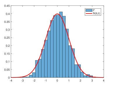
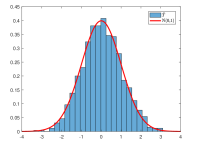
Figure 1: Histogram plots of the test statistic and the standard normal distribution. Left: $P$ is known; Right: $P$ is unknown.

3.2 Type I and type II errors

In this simulation, we examine the type I error of the proposed test under the null hypothesis and the power against the alternative distributions. The edge probability between communities $k$ and $l$ is 0.2+0.4$\times I(k=l)$. The membership vector $g$ is generated by sampling each entry independently from $\left\{1,...,K\right\}$ with equal probability. The network size $n=1000$, after repeatedly performing the proposed hypothesis test 200 times, the proportion of rejection at nominal level 0.05 is summarized in Table 1. It can be seen from this table that the Type I error is close to the nominal level and our test statistic is powerful.

Table 1: Proportion of rejection at nominal level 0.05 over 200 realizations.

$K_{0}$	$K=K_{0}$	$K=K_{0}+1$
2	0.04	1
3	0.06	1
4	0.05	1

Next, we compare the performance of our test statistic $\hat{T}$ with Lei [15]. For their test statistic, we also use the bootstrap correction procedure suggested in his paper. The test statistic is referred to as $TW_{1}$. We fix the network size at $n=1000$ and let both $K$ and $K_{0}$ vary from 2 to 5. We take the same parameter settings as in [15]. The edge probabilities between communities $k$ and $l$ are $B_{kl}=0.3+4\times I\{k=l\}$. The membership vector $g$ is generated by sampling each entry independently from $\{1,2,\cdots,K\}$ with equal probability.

Under 100 independent replications, the proportion of rejection at the nominal significance level of 0.05 can be seen in Table 2. It can be seen from Table 2 that the two tests have comparable Type I and Type II errors. Here * represents alternatives that are not considered since we only consider a one-sided test with the alternative $H_{1}:K>K_{0}$.

Table 2: Proportion of rejection at nominal level 0.05 over 100 realizations.

	$\hat{T}$				$TW_{1}$
$K$	2	3	4	5	2	3	4	5
$K_{0}=2$	$\bf{0.05}$	1.00	1.00	1.00	$\bf{0.04}$	1.00	1.00	1.00
$K_{0}=3$	*	$\bf{0.05}$	1.00	1.00	*	$\bf{0.07}$	1.00	1.00
$K_{0}=4$	*	*	$\bf{0.02}$	1.00	*	*	$\bf{0.03}$	1.00
$K_{0}=5$	*	*	*	$\bf{0.05}$	*	*	*	$\bf{0.06}$

3.3 Estimating $K$ by algorithm 1

In the third simulation, we examine the performance of algorithm 1. The edge probabilities between communities $k$ and $l$ are $B_{kl}=r(3+4\times I\{k=l\})$, where $r$ controls the sparsity of the network. We consider $r\in\{0.01,0.05,0.1\}$, and values of $K$ vary from 2 to 5. The membership vector $g$ is generated by sampling each entry independently from $\{1,2,\cdots,K\}$ with equal probability. For each of $K$ and $r$, we generate 200 independent adjacency matrices $A$ with network size $n=1000$. The proportion of correct estimates can be seen in Table 3. It can be seen from Table 3 that algorithm 1 works well for $K=2,3$ at all sparsity levels. When $K$ gets larger, $K=4,5$, algorithm 1 requires a dense network to have good performance.

Table 3: Proportion of correct estimates of $K$ over 200 repetitions under different sparsity levels indexed by $r$.

$r$	0.01	0.05	0.1
$K=2$	1	1	1
$K=3$	1	1	0.99
$K=4$	0.26	0.95	0.99
$K=5$	0.00	0.87	0.93

4 Real Data Example

4.1 The dolphin network

In this subsection we turn our attention to a popularly studied network collected by Lusseau et al. [18] (The original data can be downloaded from http://www-personal.umich.edu/~mejn/netdata/). The nodes are the bottlenose dolphins of a bottlenose dolphin community living off Doubtful Sound, a fjord in New Zealand, it has 62 nodes and 159 edges. Every time a school of dolphins was encountered in the fjord between 1995 and 2001, each adult member of the school was photographed and identified from natural markings on the dorsal fin. This information was utilized to determine how often two individuals were seen together. Lusseau et al. then built a social network with 62 dolphins and 159 undirected ties representing preferred companionship. At first it is well believed that this network can be divided into two groups. Now it was argued in [17] that $K=4$ is also reasonable. The p-values corresponding to $K\in\{2,3,4\}$ are listed in Table 4. In Figure 2 we present the community detection results that are obtained by using different $K$.

Table 4: p-values corresponding to $K\in\{2,3,4\}$.

$K$	2	3	4
p-value	$1.6\times 10^{-6}$	$2.5\times 10^{-6}$	0.0014

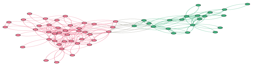
(a) $K=2$

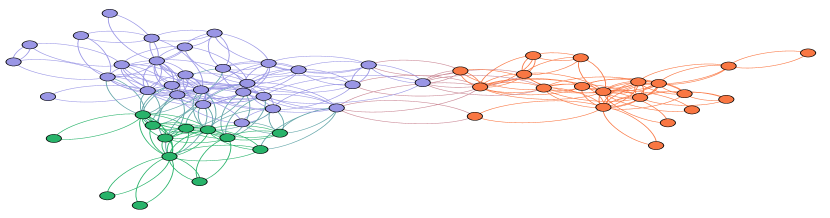
(b) $K=3$

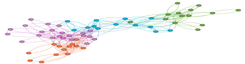
(c) $K=4$

Figure 2: Community detection results for different $K$.

4.2 The political blog data

In this subsection we consider a well-known network collected by Adamic [2] (The original data is freely available from the website http://www-personal.umich.edu/~mejn/netdata/). The nodes in this network represent political blogs and edges represent hyperlinks between blogs. The network data records hyperlinks between web blogs shortly before the 2004 US presidential election. As it is commonly done in the literature [25, 29] we only consider the largest connected component of this network, which consists of 1222 nodes. This network can be divided into two groups: the liberal and conservative communities, but there exist high degree nodes (see Figure 3), so it is more proper to fit this network by the degree corrected block model [15, 14]. Under $K=2$, we derived the $p$-value is 0. As result it is inappropriate to fit this network by the SBM with two communities.

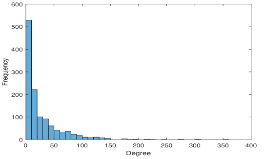
Figure 3: Degree histograms for the political blog network.

5 Technical proofs

In this section, we will prove Theorems 1-2. We first introduce some definitions and recent progress in random matrix theory(RMT).

Let $W$ be an $n\times n$ Wigner matrix with eigenvalues $\lambda_{i}$, $i=1,2,\cdots,n$. The empirical spectral distribution (ESD) of $W$ is defined as

$$F_{n}(x)=\frac{1}{n}\sum_{i=1}^{n}I(\lambda_{i}\leq x),$$

It has been proved in Bai et al [4] that $F_{n}(x)$ converges to the semicircular law $F(x)$ almost surely, see the following Lemma 1, whose density is given by

$$F(dx)=\frac{1}{2\pi}\sqrt{4-x^{2}},\quad-2\leq x\leq 2.$$

Lemma 1.

(Theorem 2.9 in Bai et al. [4]). Suppose that $W_{n}=\frac{1}{\sqrt{n}}X_{n}$ is a Wigner matrix and the entries above or on the diagonal of $X_{n}$ are independent but may be dependent on $n$ and may not necessarily be identically distributed. Assume that all the entries of $X_{n}$ are of mean zero and variance 1 and satisfy the condition that, for any constant $\eta>0$,

$$(A.1)\quad\quad\lim\limits_{n\to\infty}\frac{1}{n^{2}}\sum_{i,j}E(|X_{i,j}|^{2})I(|X_{i,j}|\geq\eta\sqrt{n})=0.$$

Then, the ESD of $W_{n}$ converges to the semicircular law almost surely.

Let $\mathcal{U}$ be an open set of the real line that contains the interval $[-2,2]$, which is the support of the semicircular law $F$. Next define $\mathcal{A}$ to be the set of analytic functions $f:\mathcal{U}\rightarrow\mathbb{R}$, where $\mathbb{R}$ is the set of real numbers. We then consider the empirical process $G_{n}={G_{n}(f)}$ given by:

$$(A.2)\quad\quad{G_{n}(f)}=n\int_{-\infty}^{\infty}f(x)[F_{n}-F]\,(dx),\qquad f\in\mathcal{A}.$$

Under the following moment conditions(1)-(3), Wang et al. [26] proved that $G_{n}$ converges weakly to a Gaussian process, see the following Lemma 2.

(1) For all $i$, $E(|X_{i,i}|^{2})=\sigma^{2}$, for all $i<j$, $E(|X_{i,j}|^{2})=1.$

(2) $\lim_{n\rightarrow\infty}\sum_{i,j}E|X_{i,j}|^{4}=L$.

(3) For any $\eta\geq 0$ as ${n\to\infty},$

$$\frac{1}{\eta^{4}n^{2}}\sum_{i,j}E[|X_{i,j}|^{4}I(|X_{i,j}|\geq\eta\sqrt{n})]=o(1).$$

Lemma 2.

(Theorem 2.1 in Wang et al. [26]). Under conditions (1)–(3), the spectral empirical process $G_{n}=(G_{n}(f))$ indexed by the set of analytic functions $\mathcal{A}$ converges weakly in finite dimension to a Gaussian process $G:=\left\{G(f):f\in\mathcal{A}\right\}$ with mean function $E[G(f)]$ given by

$$\frac{1}{4}(f(2)+f(-2))-\frac{1}{2}\tau_{0}(f)+(\sigma^{2}-2)\tau_{2}(f)+(L-3)\tau_{4}(f),$$

and the covariance function $c(f,g):=E((G(f)-E(G(f))(G(g)-E(G(g)))$ given by

$$cov(f,g)=\frac{1}{4\pi^{2}}\int_{-2}^{2}\int_{-2}^{2}f^{{}^{\prime}}(t)g^{{}^{\prime}}(s)V(t,s)\,dtds,$$

where

$$V(t,s)=(\sigma^{2}-2+\frac{L-3}{2}ts)\sqrt{(4-t^{2})(4-s^{2})}+2\log(\frac{4-ts+\sqrt{(4-t^{2})(4-s^{2})}}{4-ts-\sqrt{(4-t^{2})(4-s^{2})}}),$$

$$\tau_{l}(f)=\frac{1}{2\pi}\int_{-\infty}^{\infty}f(2cos\theta)cos(l\theta)\,d\theta.$$

Proof of Theorem 1 First, we show that the ESD of $\widetilde{A}$ converges to the semicircular law $F(x)$ almost surely. Let $X=\sqrt{n}\widetilde{A}$. From Lemma 1, it is sufficient to prove that condition (A.1) is satisfied. For any $\eta\geq 0$, we have

$$\frac{1}{n^{2}}\sum_{i,j}E(|X_{i,j}|^{2})I(|X_{i,j}|\geq\eta\sqrt{n})=\frac{1}{n^{2}}\sum_{i,j}I(|X_{i,j}|\geq\eta\sqrt{(}n))$$

$$\leq\mathop{max}\limits_{ij}\left\{I(|X_{i,j}|\geq\eta\sqrt{n})\right\}=\mathop{max}\limits_{i\neq j}\left\{I(|X_{i,j}|\geq\eta\sqrt{n})\right\}\rightarrow 0.$$

the last equality is due to $|X_{ii}|=0$, and $|X_{ij}|=\frac{A_{ij}-P_{ij}}{\sqrt{P_{ij}(1-P_{ij})}}$ is bounded.

Second, we prove that $\widetilde{A}$ satisfies conditions (1)-(3) of Lemma 2. Since $E(|X_{i,j}|^{2})=nE(|\widetilde{A}_{i,j}|^{2})=1$ for all $i,j\in[n],$ as a result condition (1) holds. Condition (2) holds because of $E|X_{i,j}|^{4}=O(\frac{1}{n^{2}}).$ Last, we verify that condition(3) holds. For any $\eta\geq 0$, we have

$$\frac{1}{\eta^{4}n^{2}}\sum_{i,j}E[|X_{i,j}|^{4}I(|X_{i,j}|\geq\eta\sqrt{n})]\leq\frac{1}{\eta^{4}n^{2}}\sum_{i,j}(E(|X_{i,j}|^{8}))^{\frac{1}{2}}E(I(|X_{i,j}|\geq\eta\sqrt{n}))^{\frac{1}{2}}$$

$$\leq\frac{C_{1}}{\eta^{4}n^{2}}\sum_{i,j}(P(|X_{i,j}|\geq\eta\sqrt{n}))^{\frac{1}{2}}\leq\frac{C_{1}}{\eta^{4}}\mathop{max}\limits_{i,j}\left\{(P(|X_{i,j}|\geq\eta\sqrt{n}))^{\frac{1}{2}}\right\}$$

$$=\frac{C_{1}}{\eta^{4}}\mathop{max}\limits_{i\neq j}\left\{(P(|\frac{A_{i,j}-P_{ij}}{P_{ij}(1-P_{ij})}|\geq\eta\sqrt{n}))^{\frac{1}{2}},\right\}$$

$$\rightarrow 0.$$

where $C_{1}$ is the upper bound of $(E(|X_{i,j}|^{8}))^{\frac{1}{2}}$, the second inequality holds because of Hölder inequality.

Let $f(x)=x^{3}$, then we have

$${G_{n}(f)}=n\int_{-\infty}^{\infty}f(x)[F_{n}-F]\,(dx)=n\int_{-\infty}^{\infty}x^{3}F_{n}\,(dx)-n\int_{-\infty}^{\infty}x^{3}F\,(dx)$$

$$~{}~{}\quad\quad=n\int_{-\infty}^{\infty}x^{3}F_{n}\,(dx)=\sum_{i=1}^{n}\lambda_{i}^{3}=trace(\widetilde{A}^{3}).$$

From Lemma 2 we derive

$$E(G(x^{3}))=0,Var(G(x^{3}))=6.$$

This completes the proof of Theorem 1.

Next we will prove Theorem 2 in matrix form. For simplicity, we introduce some notations used in the proof.

For two matrices A and B of the same dimension $m\times n$, the Hadamard product $A\circ B$ is a matrix with elements given by $(A\circ B)_{ij}=(A)_{ij}(B)_{ij},$ the Hadamard division $A\oslash B$ is a matrix with elements given by $(A\oslash B)_{ij}=\frac{(A)_{ij}}{(B)_{ij}},$ the Hadamard root is defined as $(A^{\circ\frac{1}{2}})_{ij}=A_{ij}^{\frac{1}{2}}$.

Proof of Theorem 2 We first denote

$$\widetilde{A}_{1}=\widetilde{A}+(P-\hat{P})\oslash(nP\circ(J_{n}-P))^{\circ\frac{1}{2}},$$ (6)

$$\widetilde{A_{1}^{{}^{\prime}}}=(A-\hat{P}+\hat{P}\circ I_{n})\oslash(nP\circ(J_{n}-P))^{\circ\frac{1}{2}}.$$ (7)

where $\circ$ represents the Hadamard product, $\oslash$ represents the Hadamard division, ${\circ\frac{1}{2}}$ represents the Hadamard root, $J_{n}$ is the $n\times n$ matrix of ones, $I_{n}$ is the $n\times n$ identify matrix.

Note that $\widetilde{A}=(A-P+P\circ I_{n})\oslash(nP\circ(J_{n}-P))^{\circ\frac{1}{2}}$, then we have

$$\widetilde{A_{1}}=\widetilde{A_{1}^{{}^{\prime}}}+((P-\hat{P})\circ I_{n})\oslash(nP\circ(J_{n}-P))^{\circ\frac{1}{2}}.$$ (8)

From assumption 1 we have $P_{ij}-\hat{P}_{ij}=O_{p}(\frac{k}{n})$, thus (8) can be expressed as

$$\widetilde{A_{1}}=\widetilde{A_{1}^{{}^{\prime}}}+O_{p}(\frac{k}{n^{\frac{3}{2}}})I_{n}.$$ (9)

Similarly, we have

$$\widetilde{A}=\widetilde{A_{1}}+O_{p}(\frac{k}{{n^{\frac{3}{2}}}})J_{n}.$$ (10)

As a result, we have

$$trace([\widetilde{A_{1}}]^{3}-[\widetilde{A_{1}^{{}^{\prime}}}]^{3})=O_{p}(\frac{k}{{n^{\frac{3}{2}}}})trace([\widetilde{A_{1}^{{}^{\prime}}}]^{2})+O_{p}(\frac{k^{2}}{{n^{3}}})trace([\widetilde{A_{1}^{{}^{\prime}}}])+O_{p}(\frac{k^{3}}{{n^{\frac{9}{2}}}})trace(I_{n}).$$

First, we have $trace(\widetilde{A^{{}^{\prime}}_{1}})=0.$ Second, one can prove that

$$trace([\widetilde{A_{1}^{{}^{\prime}}}]^{2})=\sum_{i=1}^{n}\widetilde{[A_{1}^{{}^{\prime}}}(i,i)]^{2}+\sum_{i\neq j}[\widetilde{A_{1}^{{}^{\prime}}}(i,j)]^{2}=\sum_{i\neq j}[\widetilde{A_{1}^{{}^{\prime}}}(i,j)]^{2}=O_{p}(n).$$

the last equality holds because of

$$\sum_{i\neq j}[\widetilde{A_{1}^{{}^{\prime}}}(i,j)]^{2}=\sum_{i\neq j}\frac{(A_{ij}-P_{ij})^{2}}{nP_{ij}(1-P_{ij})}+2\sum_{i\neq j}\frac{(A_{ij}-P_{ij})(P_{ij}-\hat{P}_{ij})}{nP_{ij}(1-P_{ij})}+\sum_{i\neq j}\frac{(P_{ij}-\hat{P}_{ij})^{2}}{nP_{ij}(1-P_{ij})}$$

$$~{}~{}~{}\quad\quad\quad\quad\quad=O_{p}(n)+O_{p}(k)+O_{p}(\frac{k^{2}}{n}).$$

Finally, we have

$$trace([\widetilde{A_{1}}]^{3}-[\widetilde{A_{1}^{{}^{\prime}}}]^{3})=O_{p}(\frac{k}{{\sqrt{n}}}).$$ (11)

Similarly to equation (10), one can derive

$$trace([\widetilde{A_{1}}]^{3}-[\widetilde{A}]^{3})=O_{p}(\frac{k}{{n^{\frac{3}{2}}}})trace([\widetilde{A}]^{2}J_{n})+O_{p}(\frac{k^{2}}{{n^{3}}})trace([\widetilde{A}J_{n}^{2}])+O_{p}(\frac{k^{3}}{{n^{\frac{9}{2}}}})trace(J_{n}^{3}).$$

Note that

$$trace([\widetilde{A}]^{2}J_{n})\leq\lambda_{max}([\widetilde{A}]^{2})n=O_{P}(n).$$

$$trace([\widetilde{A}]J_{n}^{2})\leq\lambda_{max}(\widetilde{A})n^{2}=O_{P}(n^{2}).$$

As a result

$$trace([\widetilde{A_{1}}]^{3}-[\widetilde{A}]^{3})=O_{p}(\frac{k}{{\sqrt{n}}}).$$ (12)

Recall that

$$\widetilde{A}^{{}^{\prime}}=(P\circ(J_{n}-P)\oslash(\hat{P}(J_{n}-\hat{P})))^{\circ\frac{1}{2}}\circ\widetilde{A_{1}^{{}^{\prime}}},$$ (13)

because of

$$(P\circ(J_{n}-P)))^{\circ\frac{1}{2}}=(\hat{P}\circ(J_{n}-\hat{P})))^{\circ\frac{1}{2}}\circ(1+O_{P}(\frac{k}{n}))J_{n}.$$ (14)

we have

$$\widetilde{A}^{{}^{\prime}}=(1+O_{P}(\frac{k}{n}))\widetilde{A_{1}^{{}^{\prime}}},$$ (15)

As a result,

$$trace([\widetilde{A^{{}^{\prime}}}]^{3})=(1+O_{P}(\frac{k}{n}))^{3}trace([\widetilde{A^{{}^{\prime}}_{1}}]^{3}).$$ (16)

Combing equation (11) and (12), we have

$$trace([\widetilde{A^{{}^{\prime}}}]^{3})=(1+O_{P}(\frac{k}{n}))^{3}(trace([\widetilde{A}]^{3})+O_{p}(\frac{k}{{\sqrt{n}}})).$$ (17)

This completes our proof.

6 Conclusion

In this paper, we propose a linear spectral statistic to test whether a network can be fitted by the SBM with $K_{0}$ communities. This test statistic is the trace of the third order for a centered and scaled adjacency matrix $A$. With some recent progress in random matrix theory, we derive the asymptotic distribution of the test statistic under the null hypothesis. Simulations and real data examples validate our theoretical results. In many real-world networks, the nodes often exhibit degree heterogeneity. This paper examines random networks using the framework of random matrix theory. Recently, there have been some results on block random matrices[5, 27], we hope those results can help us extend the test statistic in this paper to the degree corrected SBM in the future.

References

- [1] {barticle}[author] \bauthor\bsnmAbbe, \bfnmEmmanuel\binitsE. (\byear2018). \btitleCommunity Detection and Stochastic Block Models: Recent Developments. \bjournalJournal of Machine Learning Research \bvolume18 \bpages1–86. \endbibitem
- [2] {binproceedings}[author] \bauthor\bsnmAdamic, \bfnmLada A.\binitsL. A. and \bauthor\bsnmGlance, \bfnmNatalie\binitsN. (\byear2005). \btitleThe Political Blogosphere and the 2004 U.S. Election: Divided They Blog. In \bbooktitleProceedings of the 3rd International Workshop on Link Discovery. \bseriesLinkKDD ’05 \bpages36–43. \bpublisherAssociation for Computing Machinery. \endbibitem
- [3] {barticle}[author] \bauthor\bsnmAmini, \bfnmArash A.\binitsA. A., \bauthor\bsnmChen, \bfnmAiyou\binitsA., \bauthor\bsnmBickel, \bfnmPeter J.\binitsP. J. and \bauthor\bsnmLevina, \bfnmElizaveta\binitsE. (\byear2013). \btitlePseudo-Likelihood Methods for Community Detection in Large Sparse Networks. \bjournalThe Annals of Statistics \bvolume41 \bpages2097–2122. \endbibitem
- [4] {bbook}[author] \bauthor\bsnmBai, \bfnmZhidong\binitsZ. and \bauthor\bsnmSilverstein, \bfnmJack W.\binitsJ. W. (\byear2010). \btitleSpectral Analysis of Large Dimensional Random Matrices, \beditionsecond ed. \bseriesSpringer Series in Statistics. \bpublisherSpringer, New York. \endbibitem
- [5] {bmisc}[author] \bauthor\bsnmBao, \bfnmZhigang\binitsZ., \bauthor\bsnmHu, \bfnmJiang\binitsJ., \bauthor\bsnmXu, \bfnmXiaocong\binitsX. and \bauthor\bsnmZhang, \bfnmXiaozhuo\binitsX. (\byear2022). \btitleSpectral Statistics of Sample Block Correlation Matrices. \endbibitem
- [6] {barticle}[author] \bauthor\bsnmBickel, \bfnmPeter\binitsP., \bauthor\bsnmChoi, \bfnmDavid\binitsD., \bauthor\bsnmChang, \bfnmXiangyu\binitsX. and \bauthor\bsnmZhang, \bfnmHai\binitsH. (\byear2013). \btitleAsymptotic Normality of Maximum Likelihood and Its Variational Approximation for Stochastic Blockmodels. \bjournalThe Annals of Statistics \bvolume41 \bpages1922–1943. \endbibitem
- [7] {barticle}[author] \bauthor\bsnmBickel, \bfnmPeter J.\binitsP. J. and \bauthor\bsnmSarkar, \bfnmPurnamrita\binitsP. (\byear2016). \btitleHypothesis Testing for Automated Community Detection in Networks. \bjournalJournal of the Royal Statistical Society: Series B (Statistical Methodology) \bvolume78 \bpages253–273. \endbibitem
- [8] {barticle}[author] \bauthor\bsnmDong, \bfnmZhishan\binitsZ., \bauthor\bsnmWang, \bfnmShuangshuang\binitsS. and \bauthor\bsnmLiu, \bfnmQun\binitsQ. (\byear2020). \btitleSpectral Based Hypothesis Testing for Community Detection in Complex Networks. \bjournalInformation Sciences \bvolume512 \bpages1360–1371. \endbibitem
- [9] {barticle}[author] \bauthor\bsnmHolland, \bfnmPaul W.\binitsP. W., \bauthor\bsnmLaskey, \bfnmKathryn Blackmond\binitsK. B. and \bauthor\bsnmLeinhardt, \bfnmSamuel\binitsS. (\byear1983). \btitleStochastic Blockmodels: First Steps. \bjournalSocial Networks \bvolume5 \bpages109–137. \endbibitem
- [10] {barticle}[author] \bauthor\bsnmJalan, \bfnmSarika\binitsS. and \bauthor\bsnmBandyopadhyay, \bfnmJayendra N.\binitsJ. N. (\byear2007). \btitleRandom Matrix Analysis of Complex Networks. \bjournalPhysical Review E \bvolume76 \bpages046107. \endbibitem
- [11] {barticle}[author] \bauthor\bsnmJi, \bfnmPengsheng\binitsP. and \bauthor\bsnmJin, \bfnmJiashun\binitsJ. (\byear2016). \btitleCoauthorship and Citation Networks for Statisticians. \bjournalThe Annals of Applied Statistics \bvolume10 \bpages1779–1812. \endbibitem
- [12] {barticle}[author] \bauthor\bsnmJin, \bfnmJiashun\binitsJ. (\byear2015). \btitleFast Community Detection by SCORE. \bjournalThe Annals of Statistics \bvolume43 \bpages57–89. \endbibitem
- [13] {bbook}[author] \bauthor\bsnmJohnson, \bfnmRichard A.\binitsR. A. and \bauthor\bsnmWichern, \bfnmDean W.\binitsD. W. (\byear2007). \btitleApplied Multivariate Statistical Analysis, \bedition6th edition ed. \bpublisherPearson, \baddressUpper Saddle River, N.J. \endbibitem
- [14] {barticle}[author] \bauthor\bsnmKarrer, \bfnmBrian\binitsB. and \bauthor\bsnmNewman, \bfnmM. E. J.\binitsM. E. J. (\byear2011). \btitleStochastic Blockmodels and Community Structure in Networks. \bjournalPhysical Review E \bvolume83 \bpages016107. \endbibitem
- [15] {barticle}[author] \bauthor\bsnmLei, \bfnmJing\binitsJ. (\byear2016). \btitleA Goodness-of-Fit Test for Stochastic Block Models. \bjournalAnnals of Statistics \bvolume44 \bpages401–424. \bmrnumberMR3449773 \endbibitem
- [16] {barticle}[author] \bauthor\bsnmLei, \bfnmJing\binitsJ. and \bauthor\bsnmRinaldo, \bfnmAlessandro\binitsA. (\byear2015). \btitleConsistency of Spectral Clustering in Stochastic Block Models. \bjournalAnnals of Statistics \bvolume43 \bpages215–237. \bmrnumberMR3285605 \endbibitem
- [17] {barticle}[author] \bauthor\bsnmLiu, \bfnmWei\binitsW., \bauthor\bsnmJiang, \bfnmXingpeng\binitsX., \bauthor\bsnmPellegrini, \bfnmMatteo\binitsM. and \bauthor\bsnmWang, \bfnmXiaofan\binitsX. (\byear2016). \btitleDiscovering Communities in Complex Networks by Edge Label Propagation. \bjournalScientific Reports \bvolume6 \bpages22470. \endbibitem
- [18] {barticle}[author] \bauthor\bsnmLusseau, \bfnmDavid\binitsD., \bauthor\bsnmSchneider, \bfnmKarsten\binitsK., \bauthor\bsnmBoisseau, \bfnmOliver J.\binitsO. J., \bauthor\bsnmHaase, \bfnmPatti\binitsP., \bauthor\bsnmSlooten, \bfnmElisabeth\binitsE. and \bauthor\bsnmDawson, \bfnmSteve M.\binitsS. M. (\byear2003). \btitleThe Bottlenose Dolphin Community of Doubtful Sound Features a Large Proportion of Long-Lasting Associations. \bjournalBehavioral Ecology and Sociobiology \bvolume54 \bpages396–405. \endbibitem
- [19] {barticle}[author] \bauthor\bsnmMa, \bfnmXiaoke\binitsX., \bauthor\bsnmWang, \bfnmBingbo\binitsB. and \bauthor\bsnmYu, \bfnmLiang\binitsL. (\byear2018). \btitleSemi-Supervised Spectral Algorithms for Community Detection in Complex Networks Based on Equivalence of Clustering Methods. \bjournalPhysica A: Statistical Mechanics and its Applications \bvolume490 \bpages786–802. \endbibitem
- [20] {bbook}[author] \bauthor\bsnmNewman, \bfnmMark\binitsM. (\byear2018). \btitleNetworks. \bpublisherOxford university press. \endbibitem
- [21] {barticle}[author] \bauthor\bsnmNewman, \bfnmM. E. J.\binitsM. E. J. (\byear2006). \btitleFinding Community Structure in Networks Using the Eigenvectors of Matrices. \bjournalPhysical Review E. Statistical, Nonlinear, and Soft Matter Physics \bvolume74 \bpages036104, 19. \bmrnumber2282139 \endbibitem
- [22] {barticle}[author] \bauthor\bsnmNewman, \bfnmM. E. J.\binitsM. E. J. and \bauthor\bsnmLeicht, \bfnmE. A.\binitsE. A. (\byear2007). \btitleMixture Models and Exploratory Analysis in Networks. \bjournalProceedings of the National Academy of Sciences \bvolume104 \bpages9564. \endbibitem
- [23] {barticle}[author] \bauthor\bsnmPontes, \bfnmBeatriz\binitsB., \bauthor\bsnmGiráldez, \bfnmRaúl\binitsR. and \bauthor\bsnmAguilar-Ruiz, \bfnmJesús S.\binitsJ. S. (\byear2015). \btitleBiclustering on Expression Data: A Review. \bjournalJournal of Biomedical Informatics \bvolume57 \bpages163–180. \endbibitem
- [24] {barticle}[author] \bauthor\bsnmvon Luxburg, \bfnmUlrike\binitsU. (\byear2007). \btitleA Tutorial on Spectral Clustering. \bjournalStatistics and Computing \bvolume17 \bpages395–416. \endbibitem
- [25] {barticle}[author] \bauthor\bsnmWang, \bfnmY. X. Rachel\binitsY. X. R. and \bauthor\bsnmBickel, \bfnmPeter J.\binitsP. J. (\byear2017). \btitleLikelihood-Based Model Selection for Stochastic Block Models. \bjournalAnnals of Statistics \bvolume45 \bpages500–528. \bmrnumberMR3650391 \endbibitem
- [26] {barticle}[author] \bauthor\bsnmWang, \bfnmZhenggang\binitsZ. and \bauthor\bsnmYao, \bfnmJianfeng\binitsJ. (\byear2021). \btitleOn a Generalization of the CLT for Linear Eigenvalue Statistics of Wigner Matrices with Inhomogeneous Fourth Moments. \bjournalRandom Matrices: Theory and Applications. \endbibitem
- [27] {bmisc}[author] \bauthor\bsnmWang, \bfnmZhenggang\binitsZ. and \bauthor\bsnmYao, \bfnmJianfeng\binitsJ. (\byear2021). \btitleCentral Limit Theorem for Linear Spectral Statistics of Block-Wigner-type Matrices. \endbibitem
- [28] {barticle}[author] \bauthor\bsnmWestveld, \bfnmAnton H.\binitsA. H. and \bauthor\bsnmHoff, \bfnmPeter D.\binitsP. D. (\byear2011). \btitleA Mixed Effects Model for Longitudinal Relational and Network Data, with Applications to International Trade and Conflict. \bjournalThe Annals of Applied Statistics \bvolume5. \endbibitem
- [29] {barticle}[author] \bauthor\bsnmZhao, \bfnmYunpeng\binitsY., \bauthor\bsnmLevina, \bfnmElizaveta\binitsE. and \bauthor\bsnmZhu, \bfnmJi\binitsJ. (\byear2012). \btitleConsistency of Community Detection in Networks under Degree-Corrected Stochastic Block Models. \bjournalThe Annals of Statistics \bvolume40 \bpages2266–2292. \endbibitem