Unsupervised Inference of Signed Distance Functions from Single Sparse Point Clouds without Learning Priors

Abstract

It is vital to infer signed distance functions (SDFs) from 3D point clouds. The latest methods rely on generalizing the priors learned from large scale supervision. However, the learned priors do not generalize well to various geometric variations that are unseen during training, especially for extremely sparse point clouds. To resolve this issue, we present a neural network to directly infer SDFs from single sparse point clouds without using signed distance supervision, learned priors or even normals. Our insight here is to learn surface parameterization and SDFs inference in an end-to-end manner. To make up the sparsity, we leverage parameterized surfaces as a coarse surface sampler to provide many coarse surface estimations in training iterations, according to which we mine supervision and our thin plate splines (TPS) based network infers SDFs as smooth functions in a statistical way. Our method significantly improves the generalization ability and accuracy in unseen point clouds. Our experimental results show our advantages over the state-of-the-art methods in surface reconstruction for sparse point clouds under synthetic datasets and real scans.The code is available at https://github.com/chenchao15/NeuralTPS.

1 Introduction

Signed distance functions (SDFs) have been a popular 3D representation that shows impressive performance in various tasks [68, 15, 42, 77, 22, 4, 1, 7, 44, 31, 57, 84, 2, 3, 80, 12, 50, 21, 30, 41, 64, 62, 17, 35, 47, 34, 69]. An SDF describes a signed distance field as a mapping from a coordinate to a signed distance, and represents a surface as a level set of the field. We can learn SDFs from signed distance supervision using coordinate-based neural networks. However, obtaining the signed distance supervision requires continuous surfaces such as water-tight manifolds, hence it is still challenging to infer signed distance supervision from raw point clouds due to the discrete character.

Current methods [51, 56, 28, 58, 55, 50, 21, 30, 41, 64, 62, 17, 36] mainly leverage priors to infer SDFs for point clouds. They learn priors from well established signed distance supervision around point clouds during training, and then generalize the learned priors to infer SDFs for unseen point clouds during testing. Although local priors learned at a part level [73, 65, 9, 31, 7, 45] improve the generalization of global priors learned at a shape level [50, 21, 30, 41, 64, 62, 17, 60], the geometric variations that local priors can cover are still limited. Hence, some methods [22, 1, 84, 2, 3, 80, 44, 14] try to directly infer SDFs from single point clouds using various strategies [44, 22, 1, 84, 2, 12]. However, they require dense point clouds to assure the inference performance, which drastically limits their performance with sparse point clouds in real scans. Therefore, how to infer SDFs from sparse point clouds to achieve better generalization is still a challenge.

To overcome this challenge, we introduce a neural network to infer SDFs from single sparse point clouds. Our novelty lies in the way of inferring SDFs without signed distance supervision, learned priors or even normals, which significantly improves the generalization ability and accuracy in unseen point clouds. We achieve this by learning surface parameterization and SDF inference in an end-to-end manner using a neural network that overfits a single sparse point cloud. To make up the sparsity, the end-to-end learning turns parameterized surfaces as a coarse surface sampler which produces many coarse surface estimations on the fly to statistically infer the SDF. To target extremely sparse point clouds, we parameterize the surface of a point cloud as a single patch on a 2D plane, where 2D samples can be mapped to 3D points that lead to a coarse surface estimation. We further leverage the estimated coarse surface as a reference to infer the SDF based on thin plate splines (TPS) in the feature space, which produces smooth signed distance fields. Our method can statistically infer the SDFs from the permutation of coarse surfaces in different iterations, which reduces the effect of inaccuracy brought by each single coarse surface. Our method outperforms the latest methods under the widely used benchmarks. Our contributions are listed below.

1. We introduce a neural network to infer SDFs from single sparse point clouds without using signed distance supervision, learned priors or even normals.

2. We justify the feasibility of learning surface parameterization and inferring SDFs from sparse point clouds in an end-to-end manner. We provide a novel perspective to use surface parameterization to mine supervision.

3. Our method outperforms the state-of-the-art methods in surface reconstruction for sparse point clouds under the widely used benchmarks.

2 Related Work

Neural implicit representations have achieved promising performance in various tasks [52, 54, 24, 26, 11, 76, 72, 63, 48, 59, 25, 27]. We can learn neural implicit representations from different supervision including 3D supervision [51, 56, 55, 49, 13], multi-view [61, 40, 32, 82, 39, 75, 53, 37, 79, 78, 19, 70, 81, 71, 67, 68], and point clouds [73, 38, 50, 21]. We focus on reviewing works related to point clouds below.

Data-Driven based Methods. With 3D supervision, most methods adopted data-driven strategy to learn priors, and generalized the learned priors to infer implicit representations for unseen point clouds. Some methods learned global priors [50, 21, 30, 41, 64, 62, 17] at a shape level. To improve the generalization of learned priors, some methods learned local priors [73, 65, 9, 31, 7, 45] at a part or patch level. With the learned priors, we can infer implicit representations for unseen point clouds, and then leverage the marching cubes algorithm [43] to reconstruct surfaces.

These methods rely on a large scale dataset to learn priors while they may not generalize well to unseen point clouds that have large geometric variations from the samples in the large scale dataset.

Overfitting based Methods. For better generalization, some methods focus on learning implicit functions by overfitting neural networks on single point clouds. These methods introduce novel constraints [22, 1, 84, 2, 80, 3], ways of leveraging gradients [44, 14], differentiable poisson solver [57] or specially designed priors [45, 46] to learn signed [44, 22, 1, 84, 2, 12] or unsigned distance functions [14, 85]. Although these methods have made great progress without learning priors, they require dense point clouds to infer the distance or occupancy fields around point clouds.

Learning from Sparse Point Clouds. With sparsity, the gap between points on surfaces makes it hard to accurately infer implicit functions. Some methods learned priors [7, 45], and conducted test-stage optimization on unseen sparse point clouds [45]. Without priors, NeedleDrop [6] was proposed to infer occupancy fields by learning whether a dropped needle goes across the surface or not. However, this self-supervision is not accurate at any point on a surface and heavily relies on the length of needle. VIPSS [29] learns an implicit function from an unoriented point set based on Hermite interpolation, which is sensitive to parameter settings.

Our method falls in this category, but we aim to infer SDFs without learning priors or supervision. We achieve this by learning surface parameterization and SDFs inference in an end-to-end manner for capture a better sense on surfaces.

Neural Splines. Splines have been widely used in image manipulation [83] or generation [16]. NeuralSpline was proposed to fit point clouds with normals using implicit functions [74]. With normals, it simply infers occupancy of points on the normals, hence it focuses on fitting rather than inference. Instead, we target a more challenging scenario where we focus on inferring SDF without normals or learned priors.

3 Method

Overview. We aim to infer an SDF $f_{\theta}$ from a single sparse point cloud $\mathcal{P}=\{p_{i}|i\in[1,I]\}$, where the SDF is parameterized by a network with parameters $\theta$. At any location $q$ in 3D space, SDF $f_{\theta}$ predicts signed distance $d=f_{\theta}(q)$. Our method learns surface parameterization and SDF inference in an end-to-end manner, where we aims to use surface parameterization as a coarse surface estimation sampler to provide supervision for SDF inference. as illustrated in Fig. 1.

During surface parameterization in Fig. 1 (a), we randomly sample two sets of 2D points $\mathcal{U}$ and $\mathcal{U}^{\prime}$ in a unit square in each iteration. We map each 2D sample into a 3D point using a neural network $f_{\phi}$. This mapping leads to two sets of 3D points $\mathcal{S}=\{s_{j}|j\in[1,J]\}$ and $\mathcal{G}=\{g_{k}|k\in[1,K]\}$, each of which forms a chart covering the whole shape. We use point cloud $\mathcal{P}$ to regulate $\{s_{j}\}$, and use $\{g_{k}|k\in[1,K]\}$ to mine supervision to infer SDF $f_{\theta}$ in the following.

We leverage a thin plate splines (TPS) based network (NeuralTPS) to infer SDF $f_{\theta}$ in Fig. 1 (b). Our network learns a feature space, where we leverage TPS interpolation to produce features of arbitrary queries $q\in\mathcal{Q}$ in 3D space based on the features of sparse point cloud $\mathcal{P}$. Our network predicts signed distances $f_{\theta}(q)$ at $q$ from its interpolated feature. We infer SDF $f_{\theta}$ by minimizing the difference between the surface $\mathcal{Q}^{\prime}$ produced with the current inferred signed distance field and the chart $\mathcal{G}$ from the parameterized surface. Moreover, we also regulate $f_{\theta}$ by constraining sparse point cloud $\mathcal{P}$ to locate on the zero level of the SDF $f_{\theta}$.

To remedy the inaccuracy in $\mathcal{G}$, we regard $\mathcal{G}$ in each iteration as a sample of coarse surface estimation, and infer $f_{\theta}$ by minimizing the loss expectation in a statistical manner. Moreover, we introduce a confidence weight to consider the confidence of each point in $\mathcal{G}$.

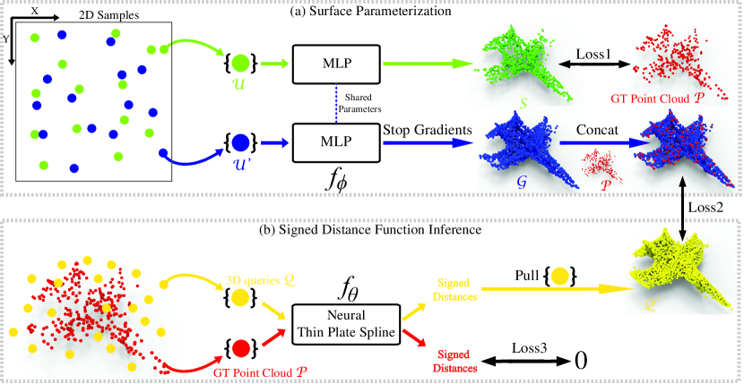
Figure 1: The overview of our method.

Surface Parameterization. We learn to parameterize a surface represented by a sparse point cloud $\mathcal{P}$ on a 2D plane in Fig. 1 (a). We leverage an MLP $f_{\phi}$ with five layers to learn a mapping from a 2D sample to a 3D point. This mapping produces a 3D chart $\mathcal{S}$ using a set of randomly sampled 2D points $\mathcal{U}$, $\mathcal{S}=f_{\phi}(\mathcal{U})$. We regulate this mapping by covering $\mathcal{S}$ onto the ground truth points $\mathcal{P}$, which maximizes the overlapping between $\mathcal{S}$ and $\mathcal{P}$ using a Chamfer Distance (CD) loss,

$$L_{CD}=\frac{1}{J}\sum_{s\in\mathcal{S}}\min_{p\in\mathcal{P}}||s-p||_{2}^{2}+\frac{1}{I}\sum_{p\in\mathcal{P}}\min_{s\in\mathcal{S}}||p-s||_{2}^{2}.\vspace{-0.05in}$$ (1)

Our parameterization is similar to AtlasNet [23]. The difference lies in the number of patches to represent a single point cloud. To remedy the sparsity, we only leverage one patch to cover the shape rather than multiple patches in AtlasNet, so that we can better fill the gaps between sparse points using generated points. We visualize the effect of patch numbers in Fig. 2, where each subfigure shows a point cloud with the same number of points but different number of patches. The comparison indicates that more patches can not fill the gaps among points, while our single chart reveals a more compact surface.

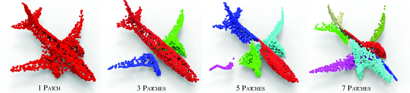
Figure 2: The effect of patch numbers.

With surface parameterization, we regard our MLP as a coarse surface sampler which predicts an additional coarse surface estimation $\mathcal{G}$ using another set of 2D samples $\mathcal{U}^{\prime}$, $\mathcal{G}=f_{\phi}(\mathcal{U}^{\prime})$. In each iteration during training, we leverage $\mathcal{G}$ to infer SDF $f_{\theta}$ in Fig. 1 (b). We stop the gradients that can be back-propagated from the loss on $\mathcal{G}$, which avoids the impact of SDF inference on surface parameterization. This is also the reason why we design a two-branch structure for surface parameterization, which differs our method from AtlasNet a lot.

Signed Distance Function Inference. We introduce NeuralTPS to infer SDF $f_{\theta}$ from sparse point cloud $\mathcal{P}$. We sample 3D queries $q$ using a Gaussian function centered at each point in $\mathcal{P}$. The inferred SDF predicts signed distances $f_{\theta}(p_{i})$ and $f_{\theta}(q)$ at each point $p_{i}\in\mathcal{P}$ and each sampled query $q$. Here, we impose two different constraints to signed distances $f_{\theta}(p_{i})$ on the surface and signed distances $f_{\theta}(q)$ in 3D space.

For points $p$ on surface of $\mathcal{P}$, we expect them on the zero level set of SDF $f_{\theta}$, hence we leverage a MSE loss,

$$L_{Surf}=\sum_{p\in\mathcal{P}}(f_{\theta}(p))^{2}.$$ (2)

For points $q\in\mathcal{Q}$ in 3D space, we expect the signed distance field could provide the correct signed distances and gradients which can be used to pull $q$ onto the nearest points on the coarse surface $\mathcal{G}$. Here, we use a pulling operation introduced in [44] to pull $q$ to $q^{\prime}$, $q^{\prime}=q-f_{\theta}(q)\nabla f_{\theta}(q)/||\nabla f_{\theta}(q)||_{2}$. while, different from [44], we introduce a novel confidence-weighted loss to optimize the set $\mathcal{Q}^{\prime}=\{q^{\prime}\}$ to cover the coarse surface $\mathcal{G}$ with considering the confidence of each point in $\mathcal{G}$,

$$L_{Pull}(\mathcal{Q}^{\prime},\mathcal{G})=\sum_{q^{\prime}\in\mathcal{Q}^{\prime},g\in\mathcal{G}}w||q^{\prime}-g||_{2}^{2}.$$ (3)

where $g$ is the nearest point of $q$ on $\mathcal{G}$. In practice, we find the nearest point from the union of $\mathcal{G}$ and sparse points $\mathcal{P}$. We use $w$ to model the confidence of each point $g\in\mathcal{G}$ to remedy the inaccuracy in $\mathcal{G}$. $g$ has higher confidence if it is nearer to sparse point cloud $\mathcal{P}$ and vice versa. Hence, we formulate $w$ as, $w=exp(-\delta*||g-p||_{2}^{2})$, where $p$ is the nearest point of $g$ on the sparse point cloud $\mathcal{P}$ and the decay parameter $\delta$ is set to 50 in our experiments.

To further reduce the impact of inaccuracy in $\mathcal{G}$, we minimize $L_{Pull}(\mathcal{Q}^{\prime},\mathcal{G})$ in a statical manner over $\{\mathcal{G}\}$ obtained in different iterations rather than $\mathcal{G}$ in a single iteration. Hence, we aim to find an optimal $\mathcal{Q}^{\prime}$ that has the smallest average deviation over $\{\mathcal{G}\}$. We reformulate $L_{Pull}(\mathcal{Q}^{\prime},\mathcal{G})$ into $\mathbb{E}_{\{\mathcal{G}\}}\{L_{Pull}(\mathcal{Q}^{\prime},\mathcal{G})\}$.

Loss Function. We optimize surface parameterization and SDF inference in an end-to-end manner by adjusting parameters $\theta$ and $\phi$ using the following objective function,

$$\min_{\theta,\phi}L_{CD}+\alpha L_{Surf}+\beta\mathbb{E}_{\{\mathcal{G}\}}\{L_{Pull}(\mathcal{Q}^{\prime},\mathcal{G})\},\vspace{-0.05in}$$ (4)

where $\alpha$ and $\beta$ are balance weights, and we set $\alpha=0.1$ and $\beta=0.1$ in our experiments.

Neural Thin Plate Splines. We introduce NeuralTPS to infer SDF as a smooth function. Our key idea is to learn an optimal feature space that can be further mapped to signed distances, where we regress signed distances at queries using features of surface points by TPS interpolation.

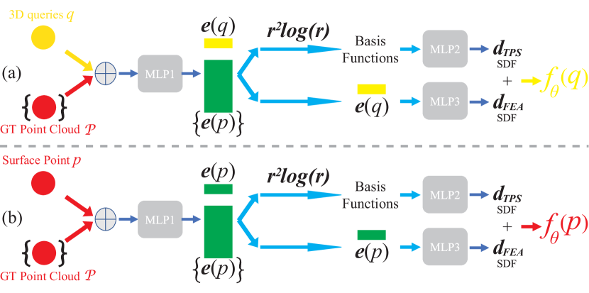
Figure 3: The illustration of NeuralTPS with one query, such as (a) a surface point or (b) a sampled point.

We illustrate NeuralTPS in Fig. 3 (a). We start from concatenating surface point $p_{i}\in\{\mathcal{P}\}$ with sampled queries $q\in\mathcal{Q}$ in each iteration. This aims to extract point features $\mathbf{e}(p_{i})$ and $\mathbf{e}(q)$ using the same parameters for TPS interpolation. So, we leverage an MLP (denoted as MLP1) to learn features of points $p_{i}$ and query $q$, i.e. $\mathbf{e}(p_{i})=MLP(p_{i})$ and $\mathbf{e}(q)=MLP(q)$. Then, we regard the features of surface points as control nodes to regress signed distances $d_{TPS}$ at queries $q$ using TPS interpolation below,

$$d_{TPS}=\sum_{i=1}^{I}c_{i}\psi(||\mathbf{e}(p_{i})-\mathbf{e}(q)||_{2}^{2}),$$ (5)

where $\psi(r)=r^{2}log(r)$ is known as the thin plate radial basis function, and we will report results with other basis functions in our experiments. $\{c_{i}\}$ are weights for integrating basis functions, which are learnable parameters in another MLP (denoted as MLP2).

To complement the potential interpolation error in the linear summation, we predict a displacement $d_{FEA}$ for signed distances at queries using point features $\mathbf{e}(q)$ through an MLP (denoted as MLP3). In summary, we formulate signed distances at queries $q$ as,

$$f_{\theta}(q)=d_{TPS}+d_{FEA}.$$ (6)

We use the same way to predict signed distance $f_{\theta}(p)$ of surface points $p\in\{\mathcal{P}\}$, as illustrated in Fig. 3 (b).

Motivation of NeuralTPS. One of challenge for SDF inference from sparse point clouds is to produce a smooth field. We adopt TPS in the learned feature space, since TPS is a unique solution to scattered data interpolation with maximum smoothness evaluated by second order partial derivatives [66]. The smoothness is a measurement of the aggregate curvature of $f_{\theta}$ over the region of the surface. Since the smoothness may filter out sharp edges, we conduct TPS interpolation in the learned feature space rather than 3D space.

Details. In surface parameterization in Fig. 1, our MLP is formed by 5 fully connected layers. In each iteration during training, we sample 2D points to generate $\mathcal{S}$ with $2000$ 3D points to calculate $L_{CD}$ with the ground truth $\mathcal{P}$, and generate $\mathcal{G}$ with $5000$ 3D points to calculate $L_{Pull}$.

In NeuralTPS in Fig. 3, MLP1 is formed by 10 fully connected layers and other two MLPs are formed by 1 fully connected layer. We establish $\mathcal{Q}$ by sampling queries around each point in $\mathcal{S}$ with a Gaussian distribution, which gets more queries around the surface.

4 Experiments

We evaluate our method in surface reconstruction from synthetic point clouds and real scans. The point clouds represent shapes and scenes. For each point cloud, we predict signed distances at grid locations using the inferred SDF $f_{\theta}$, and then run the marching cubes algorithm [43] to extract a surface.

4.1 Surface Reconstruction For Shapes

Dataset and Metrics. We evaluate our method in surface reconstruction for rigid shapes and non-rigid shapes in ShapeNet [10] and D-FAUST [5]. We report our evaluations under the test splitting of ShapeNet from NeuralPull [44] and the test set of D-FAUST. We do not learn priors, and train neural network to overfit to each single point cloud. For each shape, we follow NeedleDrop [6] to randomly sample $300$ points on each shape as the input to each method in evaluations. Using the learned implicit functions, we extract meshes as the reconstructed surfaces. We evaluate the reconstructed surfaces using L1 Chamfer Distance ($CD_{L1}$), L2 Chamfer Distance ($CD_{L2}$), and normal consistency ($NC$), where we sample $100k$ points on the reconstructed surfaces and ground truth surfaces respectively to measure errors.

Evaluations. We compare our methods with the state-of-the-art methods including NeedleDrop (NDrop) [6], NeuralPull (NPull) [44], SAP [57], ShapeGF (ShpGF) [8], NeuralSplines (NSpline) [74], OnSurf [45], VIPSS [29]. Here, we do not compare with SAL [1] or IGR [22], since NDrop and NPull showed better performance over them. Except OnSurf, all other methods do not leverage priors during training, and we train all these methods to overfit to the same sparse point clouds separately. We produce the results of OnSurf using its on-surface prior which is trained under a large-scale dataset. To produce the results of ShapeGF, we use PSR [33] to reconstruct meshes from the predicted point clouds, since the code for reconstruction using gradients is not available. For the normals required by NeuralSplines as input, we provide it the normals obtained on the ground truth meshes. We also do not compare the results of NeedleDrop from its original paper, since its official code shows that it samples $300$ points from a mesh in each iteration during training, which is equivalent to observing a much denser point cloud rather than a single sparse point cloud with merely $300$ during training.

We report numerical comparisons in Tab. 1, Tab. 2, and Tab. 3. The comparisons indicate that we achieve the best results which show our superior performance over the latest methods. We also achieve better performance over OnSurf which learns priors for sparse points but does not generalize well to unseen shapes. While methods without learning priors like NeuralPull, NeedleDrop, and SAP can not learn implicit functions from merely $300$ points. Our visual comparisons in Fig. 4 highlights our advantages in reconstructing more complete and smooth surfaces.

	NDrop	NPull	SAP	ShpGF	NSpline	OnSurf	VIPSS	Ours
Plane	0.499	0.141	0.141	0.110	0.119	0.153	1.193	0.095
Chair	0.395	0.196	0.363	0.304	0.306	0.316	0.851	0.197
Cabinet	0.229	0.163	0.152	0.604	0.181	0.244	0.584	0.138
Display	0.287	0.145	0.281	0.521	0.193	0.204	0.518	0.127
Vessel	0.488	0.116	0.138	0.367	0.134	0.128	0.571	0.104
Table	0.426	0.400	0.442	0.619	0.318	0.288	1.146	0.225
Lamp	0.554	0.162	0.385	0.446	0.231	0.229	0.956	0.120
Sofa	0.259	0.139	0.151	0.655	0.168	0.147	0.451	0.125
Mean	0.392	0.183	0.257	0.453	0.206	0.214	0.784	0.141

Table 1: Accuracy of reconstruction with $300$ points under ShapeNet in terms of $CD_{L1}$ $\times$ 10.

	NDrop	NPull	SAP	ShpGF	NSpline	OnSurf	VIPSS	Ours
Plane	0.755	0.036	0.063	0.031	0.127	0.112	5.829	0.030
Chair	0.532	0.174	0.429	0.275	0.247	0.448	3.291	0.149
Cabinet	0.245	0.086	0.062	0.098	0.064	0.171	2.336	0.050
Display	0.401	0.099	0.311	0.818	0.095	0.153	2.139	0.083
Vessel	0.844	0.074	0.105	0.439	0.066	0.066	2.614	0.051
Table	0.701	0.892	0.604	1.117	0.312	0.419	5.009	0.272
Lamp	1.071	0.144	0.542	0.591	0.183	0.351	4.617	0.051
Sofa	0.463	0.072	0.073	1.253	0.053	0.066	1.890	0.056
Mean	0.627	0.197	0.274	0.578	0.143	0.223	3.47	0.093

Table 2: Accuracy of reconstruction with $300$ points under ShapeNet in terms of $CD_{L2}$ $\times$ 100.

	NDrop	NPull	SAP	ShpGF	NSpline	OnSurf	VIPSS	Ours
Plane	0.819	0.897	0.774	0.747	0.895	0.864	0.833	0.899
Chair	0.777	0.861	0.725	0.547	0.759	0.813	0.821	0.863
Cabinet	0.843	0.888	0.824	0.508	0.840	0.787	0.851	0.898
Display	0.873	0.909	0.744	0.643	0.830	0.855	0.899	0.924
Vessel	0.838	0.880	0.813	0.667	0.842	0.879	0.867	0.908
Table	0.795	0.835	0.686	0.601	0.771	0.827	0.783	0.877
Lamp	0.828	0.887	0.777	0.673	0.814	0.858	0.848	0.902
Sofa	0.808	0.905	0.817	0.508	0.828	0.881	0.882	0.919
Mean	0.823	0.883	0.770	0.612	0.822	0.845	0.848	0.899

Table 3: Accuracy of reconstruction with $300$ points under ShapeNet in terms of $NC$.

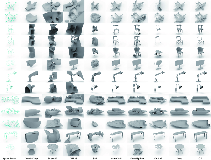
Figure 4: Visual comparison with the state-of-the-art under ShapeNet dataset.

We report our evaluations under D-FAUST in Tab. 4. We follow NeedleDrop to report $CD_{L2}$. We report the $5\%$, $50\%$, and $95\%$ percentiles of the CD between the surface reconstructions and the ground truth. Our method learns better SDFs which achieve better accuracy and smoother surfaces. This is also justified by our visual comparisons in Fig. 5.

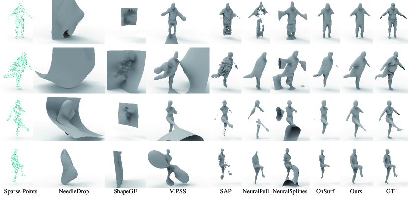
Figure 5: Visual comparison with the state-of-the-art under D-FAUST dataset.

Method	$CD_{L2}$$\times$100			NC
	5%	50%	95%
NDrop	0.126	1.000	7.404	0.792
NPull	0.018	0.032	0.283	0.877
SAP	0.014	0.024	0.071	0.852
ShpGF	0.452	1.567	8.648	0.750
NSpline	0.037	0.080	0.368	0.808
OnSurf	0.015	0.037	0.123	0.908
VIPSS	0.518	4.327	9.383	0.890
Ours	0.012	0.160	0.022	0.909

Table 4: Accuracy of reconstruction with $300$ points under D-FAUST in terms of $CD_{L2}$ and $NC$.

Method	Burghers			Copyroom			Lounge			Stonewall			Totempole			Mean
	$CD_{L1}$	$CD_{L1}$	$NC$	$CD_{L1}$	$CD_{L1}$	$NC$	$CD_{L1}$	$CD_{L1}$	$NC$	$CD_{L1}$	$CD_{L1}$	$NC$	$CD_{L1}$	$CD_{L1}$	$NC$	$CD_{L1}$	$CD_{L1}$	$NC$
PSR	0.178	0.205	0.874	0.225	0.286	0.861	0.280	0.365	0.869	0.300	0.480	0.866	0.588	1.673	0.879	0.314	0.602	0.870
NDrop	0.200	0.114	0.825	0.168	0.063	0.696	0.156	0.050	0.663	0.150	0.081	0.815	0.203	0.139	0.844	0.175	0.089	0.769
NPull	0.064	0.008	0.898	0.049	0.005	0.828	0.133	0.038	0.847	0.060	0.005	0.910	0.178	0.024	0.908	0.097	0.016	0.878
SAP	0.153	0.101	0.807	0.053	0.009	0.771	0.134	0.033	0.813	0.070	0.007	0.867	0.474	0.382	0.725	0.151	0.100	0.797
NSpline	0.135	0.123	0.891	0.056	0.023	0.855	0.063	0.039	0.827	0.124	0.091	0.897	0.378	0.768	0.892	0.151	0.209	0.889
Ours	0.055	0.005	0.909	0.045	0.003	0.892	0.129	0.022	0.872	0.054	0.004	0.939	0.103	0.017	0.935	0.077	0.010	0.897

Table 5: Accuracy of reconstruction under 3D Scene in terms of L2CD, L1CD and NC.

4.2 Surface Reconstruction For Scenes

Dataset and Metrics. We further evaluate our method in surface reconstruction for scenes in 3D Scene [86] and KITTI [20]. For results under 3D scene, we follow previous methods [44, 31] to randomly sample $100$ points per $m^{2}$. For results under KITTI dataset, we use point clouds in single frames to conduct a comparison. Similarly, we evaluate the reconstructed surfaces using L1 Chamfer Distance ($CD_{L1}$), L2 Chamfer Distance ($CD_{L2}$), and normal consistency ($NC$), where we sample $1000k$ points on the reconstructed surfaces and ground truth surfaces respectively to measure errors.

Evaluations. We compare our methods with the state-of-the-art methods including PSR [33], NeedleDrop (NDrop) [6], NeuralPull (NPull) [44], SAP [57], and NeuralSplines (NSpline) [74]. We train each method to overfit each single point cloud. Similarly, we provide NSpline the ground truth normals as input. Our numerical comparisons in Tab. 5 show that our method can reveal more accurate geometry in a 3D scene. Our reconstructed surfaces in Fig. 6 are smoother and more complete than others, and do not have artifacts in empty space as NSpline, which justifies our capability of handling sparsity in point clouds.

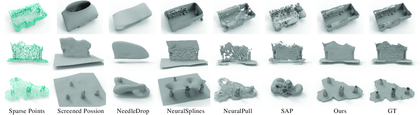
Figure 6: Visual comparison with the state-of-the-art under 3D scene dataset.

We further show our reconstructed surfaces from KITTI dataset. Since there are no ground truth meshes, we evaluate our method in visual comparisons with screened possion reconstruction (PSR) [33], NeedleDrop (NDrop) [6], NeuralPull (NPull) [44], SAP [57], and OnSurf [45]. The visual comparisons in reconstructing cars, pedestrians, and roads are shown in Fig. 8, Fig. 9 and Fig. 10. Our reconstructed surfaces show more complete surfaces with more geometry details, such as the walking poses of pedestrians, the windows of cars. The smooth roads that we construct highlight our ability of reconstructing thin structures even with sparse points. Our method does not use any learnable priors, and performs much better than the methods without learning priors, such as NeedleDrop and NeuralPull, and also OnSurf which learns a prior for sparse points.

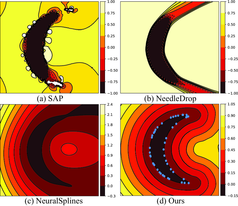
Figure 7: Visual comparison of learned fields with SAP, NeedleDrop, NeuralSplines on a 2D case.

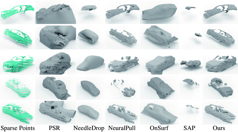
Figure 8: Visual comparisons of cars in KITTI.

4.3 Analysis

We first visualize the signed distance field that our method learns in Fig. 7. To highlight our performance, we conduct visual comparisons with SAP, NeedleDrop, and NeuralSplines on a 2D case. SAP and NeedleDrop estimate occupancy fields, while NeuralSplines and ours learn signed distance fields, and we also provide the ground truth normals to NeuralSplines to produce its results. We use each method to learn an SDF from a sparse 2D point cloud that is nonuniformly sampled on a moon like shape, where we show these points as blue dots in Fig. 7(d). The visual comparisons of level sets learned by each method indicate that our method can employ TPS to reveal smoother level sets with the highest accuracy among the counterparts. Specifically, SAP and NeedleDrop do not deal with sparsity well. Although NeuralSplines also use splines to fit signed distances, it uses the distances along normals as the ground truth, which easily produce artifacts near sharp area.

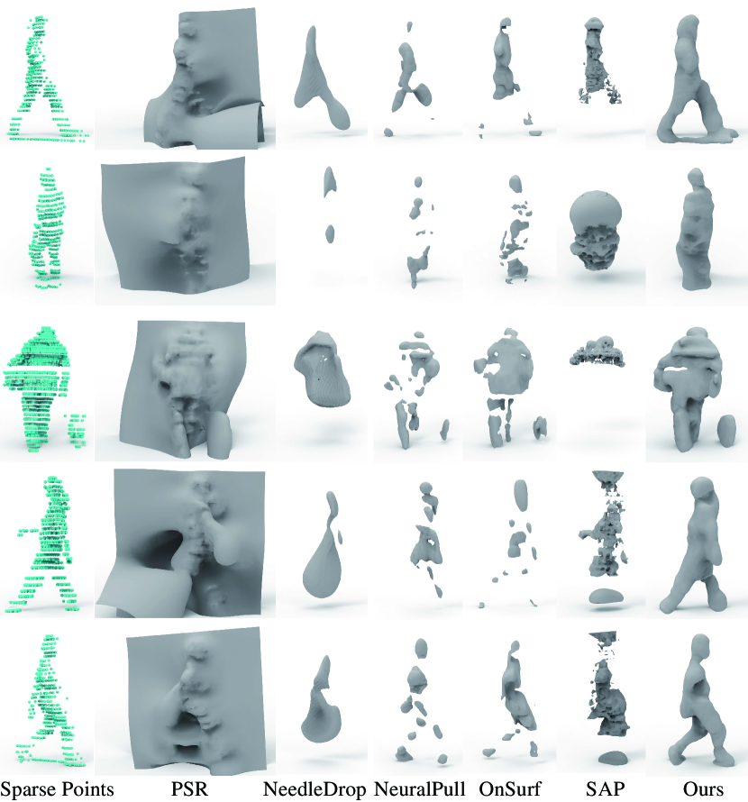
Figure 9: Visual comparisons of pedestrians in KITTI.

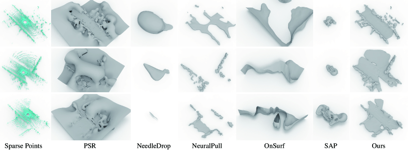
Figure 10: Visual comparisons of roads in KITTI.

4.4 Ablation Studies

To justify each module of our method, we conduct our ablation studies in airplane class that we used in Sec. 4.1 under ShapeNet. We report results in surface reconstruction with different variations of our method.

Surface Parameterizations. We first highlight the benefits of end-to-end training in Tab. 6. Hence, we optimize surface parameterization and SDF inference separately, and merely use the predicted $5000$ points from surface parameterization to infer SDF, as shown by the result of “Separate”. The degenerated results show that we can infer more accurate SDFs by observing surface estimation in different iteration. Then, we replace surface parameterization into the latest point cloud upsampling method [18] to upsample the $300$ point input to $5000$ points. The result of “Upsample” indicates that the upsampling method can not generalize the learned prior to upsample $300$ points into a plausible shape with $5000$ points. As shown in Fig. 11, the upsampling method is sensitive to the density of input points, resulting in distorted shapes after upsampling. In contrast, both of our surface parameterization and the points pulled to the surface fill the gaps of the sparse point cloud well, which leads to a smooth and complete shape. Next, we show the effect of gradient stop by turning it off. The result of “GradDiff” indicates that the error backpropagated from the SDF inference brings too much uncertainty to the surface parameterizations, which turns to degenerate the SDF inference.

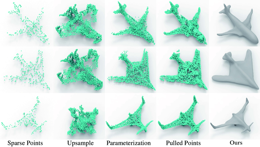
Figure 11: Visual comparisons of surface parameterizations.

	Separate	Upsample	GradDiff	Ours
$CD_{L1}$$\times$10	0.105	0.582	0.102	0.095
$CD_{L2}$$\times$100	0.118	0.815	0.047	0.030
$NC$	0.891	0.724	0.897	0.899

Table 6: Effect of surface parameterization.

We conduct experiments to explore the effect of using more patches for surface parameterizations. As shown in Fig. 2, we use more branches like AtlasNet [23] to cover the surface by generating more patches, such as $\{1,3,5\}$. The comparison in Tab. 7 shows that more patches degenerate reconstruction accuracy. Since more patches result in larger gaps between patches as we pointed out in Fig. 2, which does not resolve the sparsity on the surface.

	1	3	5
$CD_{L1}$$\times$10	0.095	0.114	0.115
$CD_{L2}$$\times$100	0.030	0.071	0.077
$NC$	0.899	0.898	0.896

Table 7: Effect of patch numbers.

Loss. We conduct experiments to explore the importance of each term in our loss function in Eq. 4. We remove each of them respectively, and report results in Tab. 8. Since we learn SDF, we keep $L_{Pull}$ in all experiments. We first remove $L_{CD}$ and pull queries directly on the sparse points rather than the output of surface parameterization. The degenerated results of “No $L_{CD}$” show that the surface parameterization provides an important surface estimation to infer SDFs. Then, we remove $L_{Surf}$, and get slightly worse results of “No $L_{Surf}$”. These results show the effectiveness of each term, and surface parameterizations supervised by $L_{CD}$ are the most important.

	No $L_{CD}$	No $L_{Surf}$	Ours
$CD_{L1}$$\times$10	0.146	0.108	0.095
$CD_{L2}$$\times$100	0.109	0.041	0.030
$NC$	0.844	0.898	0.899

Table 8: Effect of losses.

Thin Plate Splines. We report ablation studies related to TPS in Tab. 9. We first replace TPS $\psi(r)=r^{2}log(r)$ into other splines like $\psi(r)=|r|^{3}$. The results of “$|r|^{3}$” show that the basis function we use performs better. Then, we highlight the feature space where we do TPS interpolation by removing the MLP1 in Fig. 3. Instead, we do TPS directly in the spatial space. The result of “No Feature” drastically degenerates, which indicates it is more effective to perform TPS interpolation in an optimized feature space than in spatial space. Next, we explore the effect of the displacement $d_{FEA}$ by removing the MLP3 in Fig. 3. The result of “No Disp” shows that predicting SDFs directly from the feature is a good remedy to the TPS prediction.

	$|r|^{3}$	No Feature	No Disp	Ours
$CD_{L1}$$\times$10	0.110	0.791	0.159	0.095
$CD_{L2}$$\times$100	0.043	1.699	0.193	0.030
$NC$	0.895	0.691	0.898	0.899

Table 9: Effect of Thin Plate Splines.

Noise Levels. We report the effect of noises in our method in Tab. 10. We add Gaussian noises with standard deviations including $\{1\%,2\%,3\%\}$. Our results slightly degenerate with $1\%$ and $2\%$ noises and get much worse with $3\%$ noises. Compared to SAP, our method is more robust to noises, as shown in Fig 12 (a).

	SAP				Ours
	0%	1%	2%	3%	0%	1%	2%	3%
$CD_{L1}$$\times$10	0.141	0.254	0.332	0.561	0.095	0.103	0.177	0.272
$CD_{L2}$$\times$100	0.063	0.152	0.212	0.348	0.030	0.030	0.041	0.114
$NC$	0.774	0.645	0.622	0.601	0.899	0.878	0.835	0.803

Table 10: Effect of noise levels.

Point Number. Although our method produces good results on sparse points, we are also able to reconstruct surfaces from dense points, as shown in Fig. 12 (b).

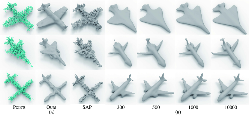
Figure 12: (a) Comparisons with noises. (b) Comparisons with different point numbers.

5 Conclusion

We present a method to infer SDFs from single sparse point clouds without using signed distance supervision, learned priors or even normals. We achieve this by learning surface parameterizations and SDF inference in an end-to-end manner. We parameterize the surface as a single chart, which significantly reduces the impact of the sparsity. By evaluating surface parameterization in different iterations, we provide a novel perspective to mine supervision from multiple coarse surface estimations for SDF inference. We also successfully leverage TPS interpolation in feature space to impose smooth constraints on inferring SDF from multiple coarse surface estimations in a statistical way. We justified the effectiveness of key modules and report results that outperform the state-of-the-art methods under the widely used benchmarks.

References

- [1] Matan Atzmon and Yaron Lipman. SAL: Sign agnostic learning of shapes from raw data. In IEEE Conference on Computer Vision and Pattern Recognition, 2020.
- [2] Matan Atzmon and yaron Lipman. SALD: sign agnostic learning with derivatives. In International Conference on Learning Representations, 2021.
- [3] Yizhak Ben-Shabat, Chamin Hewa Koneputugodage, and Stephen Gould. DiGS : Divergence guided shape implicit neural representation for unoriented point clouds. CoRR, abs/2106.10811, 2021.
- [4] Wang Bing, Yu Zhengdi, Bo Yang, Qin Jie, Breckon Toby, Shao Ling, Niki Trigoni, and Andrew Markham. Rangeudf: Semantic surface reconstruction from 3d point clouds. arXiv preprint arXiv:2204.09138, 2022.
- [5] Federica Bogo, Javier Romero, Gerard Pons-Moll, and Michael J. Black. Dynamic FAUST: Registering human bodies in motion. In IEEE Computer Vision and Pattern Recognition, 2017.
- [6] Alexandre Boulch, Pierre-Alain Langlois, Gilles Puy, and Renaud Marlet. Needrop: Self-supervised shape representation from sparse point clouds using needle dropping. In International Conference on 3D Vision, 2021.
- [7] Alexandre Boulch and Renaud Marlet. POCO: Point convolution for surface reconstruction. In IEEE Conference on Computer Vision and Pattern Recognition, pages 6302–6314, 2022.
- [8] Ruojin Cai, Guandao Yang, Hadar Averbuch-Elor, Zekun Hao, Serge Belongie, Noah Snavely, and Bharath Hariharan. Learning gradient fields for shape generation. In European Conference on Computer Vision, 2020.
- [9] Rohan Chabra, Jan Eric Lenssen, Eddy Ilg, Tanner Schmidt, Julian Straub, Steven Lovegrove, and Richard A. Newcombe. Deep local shapes: Learning local SDF priors for detailed 3D reconstruction. In European Conference on Computer Vision, volume 12374, pages 608–625, 2020.
- [10] Angel X. Chang, Thomas Funkhouser, Leonidas Guibas, Pat Hanrahan, Qixing Huang, Zimo Li, Silvio Savarese, Manolis Savva, Shuran Song, Hao Su, Jianxiong Xiao, Li Yi, and Fisher Yu. ShapeNet: An Information-Rich 3D Model Repository. Technical Report arXiv:1512.03012 [cs.GR], Stanford University — Princeton University — Toyota Technological Institute at Chicago, 2015.
- [11] Chao Chen, Zhizhong Han, Yu-Shen Liu, and Matthias Zwicker. Unsupervised learning of fine structure generation for 3D point clouds by 2D projections matching. In IEEE International Conference on Computer Vision, 2021.
- [12] Chao Chen, Yu-Shen Liu, and Zhizhong Han. Latent partition implicit with surface codes for 3d representation. In European Conference on Computer Vision, 2022.
- [13] Zhiqin Chen and Hao Zhang. Learning implicit fields for generative shape modeling. IEEE Conference on Computer Vision and Pattern Recognition, 2019.
- [14] Julian Chibane, Aymen Mir, and Gerard Pons-Moll. Neural unsigned distance fields for implicit function learning. arXiv, 2010.13938, 2020.
- [15] Angela Dai and Matthias Nießner. Neural Poisson: Indicator functions for neural fields. arXiv preprint arXiv:2211.14249, 2022.
- [16] Conor Durkan, Artur Bekasov, Iain Murray, and George Papamakarios. Neural spline flows. In Advances in Neural Information Processing Systems, pages 7509–7520, 2019.
- [17] Philipp Erler, Paul Guerrero, Stefan Ohrhallinger, Niloy J. Mitra, and Michael Wimmer. Points2Surf: Learning implicit surfaces from point clouds. In European Conference on Computer Vision, 2020.
- [18] Wanquan Feng, Jin Li, Hongrui Cai, Xiaonan Luo, and Juyong Zhang. Neural points: Point cloud representation with neural fields for arbitrary upsampling. In IEEE Conference on Computer Vision and Pattern Recognition, 2022.
- [19] Qiancheng Fu, Qingshan Xu, Yew-Soon Ong, and Wenbing Tao. Geo-Neus: Geometry-consistent neural implicit surfaces learning for multi-view reconstruction. 2022.
- [20] Andreas Geiger, Philip Lenz, and Raquel Urtasun. Are we ready for autonomous driving? the kitti vision benchmark suite. In Computer Vision and Pattern Recognition, 2012.
- [21] Kyle Genova, Forrester Cole, Daniel Vlasic, Aaron Sarna, William T. Freeman, and Thomas Funkhouser. Learning shape templates with structured implicit functions. In International Conference on Computer Vision, 2019.
- [22] Amos Gropp, Lior Yariv, Niv Haim, Matan Atzmon, and Yaron Lipman. Implicit geometric regularization for learning shapes. In International Conference on Machine Learning, volume 119 of Proceedings of Machine Learning Research, pages 3789–3799, 2020.
- [23] Thibault Groueix, Matthew Fisher, Vladimir G. Kim, Bryan C. Russell, and Mathieu Aubry. A papier-mâché approach to learning 3D surface generation. In IEEE Conference on Computer Vision and Pattern Recognition, 2018.
- [24] Zhizhong Han, Chao Chen, Yu-Shen Liu, and Matthias Zwicker. DRWR: A differentiable renderer without rendering for unsupervised 3D structure learning from silhouette images. In International Conference on Machine Learning, 2020.
- [25] Zhizhong Han, Chao Chen, Yu-Shen Liu, and Matthias Zwicker. ShapeCaptioner: Generative caption network for 3D shapes by learning a mapping from parts detected in multiple views to sentences. In ACM International Conference on Multimedia, 2020.
- [26] Zhizhong Han, Guanhui Qiao, Yu-Shen Liu, and Matthias Zwicker. SeqXY2SeqZ: Structure learning for 3D shapes by sequentially predicting 1D occupancy segments from 2D coordinates. In European Conference on Computer Vision, 2020.
- [27] Zhizhong Han, Xiyang Wang, Yu-Shen Liu, and Matthias Zwicker. Hierarchical view predictor: Unsupervised 3d global feature learning through hierarchical prediction among unordered views. In Proceedings of the 29th ACM International Conference on Multimedia, pages 3862––3871, 2021.
- [28] Jiahui Huang, Hao-Xiang Chen, and Shi-Min Hu. A neural galerkin solver for accurate surface reconstruction. ACM Trans. Graph., 41(6), 2022.
- [29] Zhiyang Huang, Nathan Carr, and Tao Ju. Variational implicit point set surfaces. ACM Transactions on Graphics, 38(4):1–13, 2019.
- [30] Meng Jia and Matthew Kyan. Learning occupancy function from point clouds for surface reconstruction. arXiv, 2010.11378, 2020.
- [31] Chiyu Jiang, Avneesh Sud, Ameesh Makadia, Jingwei Huang, Matthias Nießner, and Thomas Funkhouser. Local implicit grid representations for 3D scenes. In IEEE Conference on Computer Vision and Pattern Recognition, 2020.
- [32] Yue Jiang, Dantong Ji, Zhizhong Han, and Matthias Zwicker. SDFDiff: Differentiable rendering of signed distance fields for 3D shape optimization. In IEEE Conference on Computer Vision and Pattern Recognition, 2020.
- [33] Michael M. Kazhdan and Hugues Hoppe. Screened poisson surface reconstruction. ACM Transactions on Graphics, 32(3):29:1–29:13, 2013.
- [34] Qing Li, Huifang Feng, Kanle Shi, Yue Gao, Yi Fang, Yu-Shen Liu, and Zhizhong Han. Shs-net: Learning signed hyper surfaces for oriented normal estimation of point clouds. In Proceedings of the IEEE/CVF Conference on Computer Vsion and Pattern Recognition, 2023.
- [35] Shujuan Li, Junsheng Zhou, Baorui Ma, Yu-Shen Liu, and Zhizhong Han. Neaf: Learning neural angle fields for point normal estimation. In Proceedings of the AAAI Conference on Artificial Intelligence, 2023.
- [36] Tianyang Li, Xin Wen, Yu-Shen Liu, Hua Su, and Zhizhong Han. Learning deep implicit functions for 3D shapes with dynamic code clouds. In IEEE Conference on Computer Vision and Pattern Recognition, pages 12830–12840, 2022.
- [37] Chen-Hsuan Lin, Chaoyang Wang, and Simon Lucey. SDF-SRN: Learning signed distance 3D object reconstruction from static images. In Advances in Neural Information Processing Systems, 2020.
- [38] Minghua Liu, Xiaoshuai Zhang, and Hao Su. Meshing point clouds with predicted intrinsic-extrinsic ratio guidance. In European Conference on Computer vision, 2020.
- [39] Shichen Liu, Shunsuke Saito, Weikai Chen, and Hao Li. Learning to infer implicit surfaces without 3D supervision. In Advances in Neural Information Processing Systems, 2019.
- [40] Shaohui Liu, Yinda Zhang, Songyou Peng, Boxin Shi, Marc Pollefeys, and Zhaopeng Cui. DIST: Rendering deep implicit signed distance function with differentiable sphere tracing. In IEEE Conference on Computer Vision and Pattern Recognition, 2020.
- [41] Shi-Lin Liu, Hao-Xiang Guo, Hao Pan, Pengshuai Wang, Xin Tong, and Yang Liu. Deep implicit moving least-squares functions for 3D reconstruction. In IEEE Conference on Computer Vision and Pattern Recognition, 2021.
- [42] Xiaoxiao Long, Cheng Lin, Lingjie Liu, Yuan Liu, Peng Wang, Christian Theobalt, Taku Komura, and Wenping Wang. Neuraludf: Learning unsigned distance fields for multi-view reconstruction of surfaces with arbitrary topologies. arXiv preprint arXiv:2211.14173, 2022.
- [43] William E. Lorensen and Harvey E. Cline. Marching cubes: A high resolution 3D surface construction algorithm. Computer Graphics, 21(4):163–169, 1987.
- [44] Baorui Ma, Zhizhong Han, Yu-Shen Liu, and Matthias Zwicker. Neural-pull: Learning signed distance functions from point clouds by learning to pull space onto surfaces. In International Conference on Machine Learning, 2021.
- [45] Baorui Ma, Yu-Shen Liu, and Zhizhong Han. Reconstructing surfaces for sparse point clouds with on-surface priors. In IEEE Conference on Computer Vision and Pattern Recognition, pages 6305–6315, 2022.
- [46] Baorui Ma, Yu-Shen Liu, Matthias Zwicker, and Zhizhong Han. Surface reconstruction from point clouds by learning predictive context priors. In IEEE Conference on Computer Vision and Pattern Recognition, pages 6316–6327, 2022.
- [47] Baorui Ma, Junsheng Zhou, Yu-Shen Liu, and Zhizhong Han. Towards better gradient consistency for neural signed distance functions via level set alignment. In Proceedings of the IEEE/CVF Conference on Computer Vsion and Pattern Recognition, 2023.
- [48] Julien N. P. Martel, David B. Lindell, Connor Z. Lin, Eric R. Chan, Marco Monteiro, and Gordon Wetzstein. ACORN: adaptive coordinate networks for neural scene representation. CoRR, abs/2105.02788, 2021.
- [49] Lars Mescheder, Michael Oechsle, Michael Niemeyer, Sebastian Nowozin, and Andreas Geiger. Occupancy networks: Learning 3D reconstruction in function space. In IEEE Conference on Computer Vision and Pattern Recognition, 2019.
- [50] Zhenxing Mi, Yiming Luo, and Wenbing Tao. SSRNet: Scalable 3D surface reconstruction network. In IEEE Conference on Computer Vision and Pattern Recognition, 2020.
- [51] Mateusz Michalkiewicz, Jhony K. Pontes, Dominic Jack, Mahsa Baktashmotlagh, and Anders P. Eriksson. Deep level sets: Implicit surface representations for 3D shape inference. CoRR, abs/1901.06802, 2019.
- [52] Ben Mildenhall, Pratul P. Srinivasan, Matthew Tancik, Jonathan T. Barron, Ravi Ramamoorthi, and Ren Ng. NeRF: Representing scenes as neural radiance fields for view synthesis. In European Conference on Computer Vision, 2020.
- [53] Michael Niemeyer, Lars Mescheder, Michael Oechsle, and Andreas Geiger. Differentiable volumetric rendering: Learning implicit 3D representations without 3D supervision. In IEEE Conference on Computer Vision and Pattern Recognition, 2020.
- [54] Michael Oechsle, Songyou Peng, and Andreas Geiger. UNISURF: Unifying neural implicit surfaces and radiance fields for multi-view reconstruction. In International Conference on Computer Vision, 2021.
- [55] Amine Ouasfi and Adnane Boukhayma. Few ‘zero level set’-shot learning of shape signed distance functions in feature space. In European Conference on Computer Vision, 2022.
- [56] Jeong Joon Park, Peter Florence, Julian Straub, Richard Newcombe, and Steven Lovegrove. DeepSDF: Learning continuous signed distance functions for shape representation. In IEEE Conference on Computer Vision and Pattern Recognition, 2019.
- [57] Songyou Peng, Chiyu “Max” Jiang, Yiyi Liao, Michael Niemeyer, Marc Pollefeys, and Andreas Geiger. Shape as points: A differentiable poisson solver. In Advances in Neural Information Processing Systems, 2021.
- [58] Albert Pumarola, Artsiom Sanakoyeu, Lior Yariv, Ali Thabet, and Yaron Lipman. Visco grids: Surface reconstruction with viscosity and coarea grids. In Advances in Neural Information Processing Systems, 2022.
- [59] Konstantinos Rematas, Ricardo Martin-Brualla, and Vittorio Ferrari. Sharf: Shape-conditioned radiance fields from a single view. In International Conference on Machine Learning, 2021.
- [60] Vincent Sitzmann, Julien N.P. Martel, Alexander W. Bergman, David B. Lindell, and Gordon Wetzstein. Implicit neural representations with periodic activation functions. In Advances in Neural Information Processing Systems, 2020.
- [61] Vincent Sitzmann, Michael Zollhöfer, and Gordon Wetzstein. Scene representation networks: Continuous 3D-structure-aware neural scene representations. In Advances in Neural Information Processing Systems, 2019.
- [62] Lars Mescheder Marc Pollefeys Andreas Geiger Songyou Peng, Michael Niemeyer. Convolutional occupancy networks. In European Conference on Computer Vision, 2020.
- [63] Towaki Takikawa, Joey Litalien, Kangxue Yin, Karsten Kreis, Charles Loop, Derek Nowrouzezahrai, Alec Jacobson, Morgan McGuire, and Sanja Fidler. Neural geometric level of detail: Real-time rendering with implicit 3D shapes. In IEEE Conference on Computer Vision and Pattern Recognition, 2021.
- [64] Jiapeng Tang, Jiabao Lei, Dan Xu, Feiying Ma, Kui Jia, and Lei Zhang. SA-ConvONet: Sign-agnostic optimization of convolutional occupancy networks. In Proceedings of the IEEE/CVF International Conference on Computer Vision, 2021.
- [65] Edgar Tretschk, Ayush Tewari, Vladislav Golyanik, Michael Zollhöfer, Carsten Stoll, and Christian Theobalt. PatchNets: Patch-Based Generalizable Deep Implicit 3D Shape Representations. European Conference on Computer Vision, 2020.
- [66] Greg Turk and James F. O’Brien. Modelling with implicit surfaces that interpolate. ACM Transactions on Graphics, 21(4):855–873, 2002.
- [67] Delio Vicini, Sébastien Speierer, and Wenzel Jakob. Differentiable signed distance function rendering. ACM Transactions on Graphics, 41(4):125:1–125:18, 2022.
- [68] Jiepeng Wang, Peng Wang, Xiaoxiao Long, Christian Theobalt, Taku Komura, Lingjie Liu, and Wenping Wang. NeuRIS: Neural reconstruction of indoor scenes using normal priors. In European Conference on Computer Vision, 2022.
- [69] Meng Wang, Yu-Shen Liu, Yue Gao, Kanle Shi, Yi Fang, and Zhizhong Han. Lp-dif: Learning local pattern-specific deep implicit function for 3d objects and scenes. In Proceedings of the IEEE/CVF Conference on Computer Vsion and Pattern Recognition, 2023.
- [70] Peng Wang, Lingjie Liu, Yuan Liu, Christian Theobalt, Taku Komura, and Wenping Wang. NeuS: Learning neural implicit surfaces by volume rendering for multi-view reconstruction. In Advances in Neural Information Processing Systems, pages 27171–27183, 2021.
- [71] Yiqun Wang, Ivan Skorokhodov, and Peter Wonka. HF-NeuS: Improved surface reconstruction using high-frequency details. 2022.
- [72] Xin Wen, Peng Xiang, Zhizhong Han, Yan-Pei Cao, Pengfei Wan, Wen Zheng, and Yu-Shen Liu. Pmp-net++: Point cloud completion by transformer-enhanced multi-step point moving paths. IEEE Transactions on Pattern Analysis and Machine Intelligence, pages 1–1, 2022.
- [73] Francis Williams, Teseo Schneider, Claudio Silva, Denis Zorin, Joan Bruna, and Daniele Panozzo. Deep geometric prior for surface reconstruction. In IEEE Conference on Computer Vision and Pattern Recognition, 2019.
- [74] Francis Williams, Matthew Trager, Joan Bruna, and Denis Zorin. Neural splines: Fitting 3D surfaces with infinitely-wide neural networks. In IEEE Conference on Computer Vision and Pattern Recognition, pages 9949–9958, 2021.
- [75] Yunjie Wu and Zhengxing Sun. DFR: differentiable function rendering for learning 3D generation from images. Computer Graphics Forum, 39(5):241–252, 2020.
- [76] Peng Xiang, Xin Wen, Yu-Shen Liu, Yan-Pei Cao, Pengfei Wan, Wen Zheng, and Zhizhong Han. SnowflakeNet: Point cloud completion by snowflake point deconvolution with skip-transformer. In IEEE International Conference on Computer Vision, 2021.
- [77] Qiangeng Xu, Zexiang Xu, Julien Philip, Sai Bi, Zhixin Shu, Kalyan Sunkavalli, and Ulrich Neumann. Point-nerf: Point-based neural radiance fields. In Proceedings of the IEEE/CVF Conference on Computer Vision and Pattern Recognition, pages 5438–5448, 2022.
- [78] Lior Yariv, Jiatao Gu, Yoni Kasten, and Yaron Lipman. Volume rendering of neural implicit surfaces. In Advances in Neural Information Processing Systems, 2021.
- [79] Lior Yariv, Yoni Kasten, Dror Moran, Meirav Galun, Matan Atzmon, Basri Ronen, and Yaron Lipman. Multiview neural surface reconstruction by disentangling geometry and appearance. Advances in Neural Information Processing Systems, 33, 2020.
- [80] Wang Yifan, Shihao Wu, Cengiz Oztireli, and Olga Sorkine-Hornung. Iso-Points: Optimizing neural implicit surfaces with hybrid representations. CoRR, abs/2012.06434, 2020.
- [81] Zehao Yu, Songyou Peng, Michael Niemeyer, Torsten Sattler, and Andreas Geiger. MonoSDF: Exploring monocular geometric cues for neural implicit surface reconstruction. ArXiv, abs/2022.00665, 2022.
- [82] Sergey Zakharov, Wadim Kehl, Arjun Bhargava, and Adrien Gaidon. Autolabeling 3D objects with differentiable rendering of sdf shape priors. In IEEE Conference on Computer Vision and Pattern Recognition, 2020.
- [83] Jian Zhao and Hui Zhang. Thin-plate spline motion model for image animation. In IEEE Conference on Computer Vision and Pattern Recognition, pages 3647–3656, 2022.
- [84] Wenbin Zhao, Jiabao Lei, Yuxin Wen, Jianguo Zhang, and Kui Jia. Sign-agnostic implicit learning of surface self-similarities for shape modeling and reconstruction from raw point clouds. CoRR, abs/2012.07498, 2020.
- [85] Junsheng Zhou, Baorui Ma, Yu-Shen Liu, Yi Fang, and Zhizhong Han. Learning consistency-aware unsigned distance functions progressively from raw point clouds. In Advances in Neural Information Processing Systems (NeurIPS), 2022.
- [86] Qian-Yi Zhou and Vladlen Koltun. Dense scene reconstruction with points of interest. ACM Transactions on Graphics, 32(4):112:1–112:8, 2013.