Integrability and trajectory confinement in $\mathcal{PT}$-symmetric waveguide arrays

Abstract

We consider $\mathcal{PT}$-symmetric ring-like arrays of optical waveguides with purely nonlinear gain and loss. Regardless of the value of the gain-loss coefficient, these systems are protected from spontaneous $\mathcal{PT}$-symmetry breaking. If the nonhermitian part of the array matrix has cross-compensating structure, the total power in such a system remains bounded — or even constant — at all times. We identify two-, three-, and four-waveguide arrays with cross-compensatory nonlinear gain and loss that constitute completely integrable Hamiltonian systems.

I Introduction

The concept of $\mathcal{PT}$ symmetry, originally introduced in nonhermitian quantum mechanics Bender ; Bender_book , has led to significant developments in photonics, plasmonics, quantum optics of atomic gases, metamaterials, Bose-Einstein condensates, electronic circuitry, and acoustics Bender_book ; reviews . The $\mathcal{PT}$-symmetric equations model physical structures with a built-in balance between gain and loss.

In a linear nonhermitian system, raising the gain-loss coefficient above a critical level causes trajectories to escape to infinity. The setting in of this blow-up instability can have a detrimental effect on the structure — in optics, for example, an escaping trajectory implies an uncontrollable power hike.

Taking into account nonlinear effects and adding nonlinear corrections to the equations may arrest the blow-up through the emergence of conserved quantities confining trajectories to a finite part of the phase space Dubard . In this paper, we study a class of $\mathcal{PT}$-symmetric systems with the nonhermiticity induced entirely by the nonlinear terms. On one hand, these systems provide access to the full set of behaviours afforded by the presence of gain and loss. On the other hand, they exhibit remarkable regularity properties such as the existence of the Hamiltonian structure and trajectory confinement.

The Hamiltonian structure in a dynamical system imposes a deep symmetry between two sets of coordinates parameterising its phase space. In the presence of additional first integrals, the Hamiltonian structure establishes an even higher degree of regularity: the Liouville integrability. We identify two-, three- and four-component integrable systems with nonhermitian nonlinearities that are free from the blow-up behaviour.

The two-component complex systems that we study have the form of the nonlinear Schrödinger dimer: a discrete Schrödinger equation, defined on only two sites Hamilt_dimer ; I1 ; dimer ; Tyug_Susanto ; Jackson ; standard . The nonhermitian dimer serves as an archetypal model for a pair of optical waveguides or a pair of micro-ring resonators with gain and loss, coupled by their evanescent fields waveguides ; Miri . It also arises in the study of Bose-Einstein condensates Graefe ; BEC , plasmonics plasmonics , spintronics BC , electronic circuitry electronics and several other contexts.

The literature suggests several recipes for preventing the blow-up in dimers, including linear vs nonlinear gain-loss competition lin_nonlin ; Karthiga and nonlinear gain-loss saturation Miri ; Huerta . This paper explores cross-stimulation — an alternative mechanism that, in addition to ensuring nonsingular evolution, conserves the norm $|u|^{2}+|v|^{2}$ (interpreted as the total power of light in the optical context). We present two cross-stimulated $\mathcal{PT}$-symmetric dimers that describe completely integrable Hamiltonian systems.

The cross-stimulation is a special type of a more general notion of cross-compensation of gain and loss in a multichannel structure. To illustrate this concept, we invoke a three- and four-site discrete Schrödinger equation — the $\mathcal{PT}$-symmetric trimer and quadrimer, respectively trimer . In the optical domain, the trimer and quadrimer model an optical necklace — an array of three or four coupled waveguides or resonators. We produce examples of a completely integrable $\mathcal{PT}$-symmetric trimer and quadrimer, with solutions free from the blow-up behaviour. Similar to the dimers in the first part of this study, the nonherimiticity of these necklaces is entirely due to the nonlinear terms and has a cross-compensatory character.

The paper is organised into five sections. We start with a linear hermitian dimer with the cross-stimulating cubic gain and loss (section II). The subsequent section (section III) deals with a slightly more complex cross-stimulating system whose hermitian part is cubic itself. We uncover the hidden Hamiltonian structure of these systems, determine their integrals of motion and construct analytic solutions. An integrable $\mathcal{PT}$-symmetric trimer and quadrimer are identified in section IV. Section V summarises results of this study.

II Linear dimer with nonlinear gain and loss

II.1 Gain and loss cross-stimulation

As the gain-loss coefficient is varied, the topological structure of the phase portrait of a dimer with linear gain and loss undergoes a spontaneous change. Consider, for example, the so-called standard $\mathcal{PT}$-symmetric dimer, a model that arises in a wide range of physical contexts standard ; Tyug_Susanto ; Jackson ; I1 :

$$iu_{t}+v+|u|^{2}u =i\gamma u,$$ (1a)

$$iv_{t}+u+|v|^{2}v =-i\gamma v.$$ (1b)

As $\gamma$ is raised above the critical value $\gamma_{c}=1$, the fixed point at $u=v=0$ loses its stability and the $\mathcal{PT}$-symmetry is said to become spontaneously broken. In the symmetry-broken phase ($\gamma>1$) small initial conditions give rise to exponentially growing solutions. Since the change of behaviour concerns solutions of the linearised equations, we refer to this bifurcation as the linearised symmetry breaking.

In a generic Schrödinger dimer, trajectories resulting from the exponentially growing solutions of the linearised equations may escape to infinity. For example, in the standard dimer (1) all growing linearised solutions give rise to escaping trajectories Jackson . (Note that unbounded solutions may occur in the symmetric phase too — they just need to evolve out of large initial data Tyug_Susanto ; Jackson .)

To preclude the blow-up of small initial data, we consider a system with a hermitian linearised matrix. Furthermore, our dimer is assumed to be cross-stimulated. This means that the $u$-channel gains energy at the rate proportional to the power carried by its $v$-neighbour while the $v$ amplitude loses energy at a rate proportional to the power carried by $u$:

$$iu_{t}+v =i\gamma|v|^{2}u,$$ (2a)

$$iv_{t}+u =-i\gamma|u|^{2}v.$$ (2b)

As a result of the cross-stimulation, the total power $P=|u|^{2}+|v|^{2}$ is conserved. This keeps all trajectories — both with small and large initial data — in a finite part of the phase space.

Although the cross-stimulation may come across as a purely mathematical construct, the system (2) originates in a well-established physical context. It describes the spin-torque oscillator — an isotropic ferromagnet in an external magnetic field with polarised spin current driven through it BC . The components of the total spin vector ${\bf S}=\{X,Y,Z\}$ in the free layer of the oscillator are expressible through the complex amplitudes of the dimer’s channels:

$$X=\frac{\bar{u}v+u\bar{v}}{2},\quad Y=i\frac{\bar{u}v-u\bar{v}}{2},\quad Z=\frac{|u|^{2}-|v|^{2}}{2}.$$ (3)

The length of the vector, $\mathcal{R}=\sqrt{X^{2}+Y^{2}+Z^{2}}$, is proportional to the total power carried by the dimer,

$$\mathcal{R}=\frac{|u|^{2}+|v|^{2}}{2},$$

which is fixed by the initial condition. The direction of the vector is determined by a system of three equations BC :

$$\dot{X} =-\gamma XZ,$$ (4a)

$$\dot{Y} =-(1+\gamma Y)Z,$$ (4b)

$$\dot{Z} =Y+\gamma(R^{2}-Z^{2}),$$ (4c)

where $X,Y$ and $Z$ are considered to be functions of $\tau=2t$, and the overdot stands for the derivative w.r.t. $\tau$.

Another area of applications of the cross-stimulated dimers is the classical limit of quantum theory. A system equivalent to (2) governs the normalised state vector of the nonhermitian two-level atom Graefe . The corresponding Bloch-sphere dynamics obey equations (4).

II.2 Hamiltonian structure and integrability

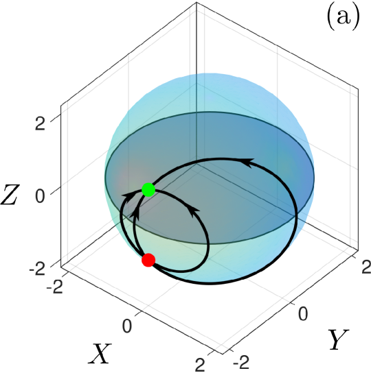
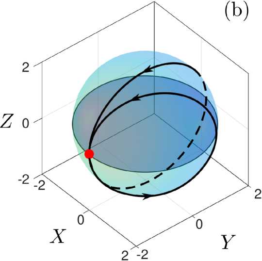
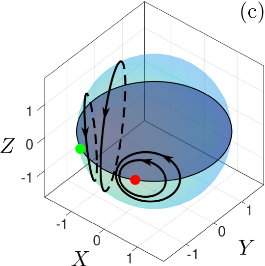
Figure 1: Trajectories of the system (4) on the surface of the sphere of the radius $\mathcal{R}>\gamma^{-1}$ (a); $\mathcal{R}=\gamma^{-1}$ (b) and $\mathcal{R}<\gamma^{-1}$ (c). (In this plot, $\gamma=\frac{1}{2}$.) Note that the largest sphere (panel a) has been scaled down while the smallest one (panel c) has been scaled up. In each ball, tinted is the equatorial plane.

Upon defining a set of polar coordinates by

$$X=e^{-\eta}\cos\theta,\quad Y=-\gamma^{-1}+e^{-\eta}\sin\theta,$$ (5)

equations (4) simplify to

$${\dot{\eta}}=\gamma Z,\quad{\dot{\theta}}=0,$$ (6)

$${\dot{Z}}=\gamma e^{-2\eta}-e^{-\eta}\sin\theta.$$ (7)

It is not difficult to see that the system (6)-(7) is Hamiltonian. We choose the integral ${\mathcal{R}}^{2}-\gamma^{-2}$ as the Hamilton function:

$$H(\eta,\theta,p_{\eta})=e^{-2\eta}-2\gamma^{-1}e^{-\eta}\sin\theta+\frac{\gamma^{2}}{4}p^{2}_{\eta}.$$ (8)

Here $\eta$ and $\theta$ are the canonical coordinates and $p_{\eta}=2\gamma^{-1}Z$ is the canonical momentum conjugate to $\eta$. The equations

$$\dot{\eta}=\frac{\partial H}{\partial p_{\eta}},\quad\dot{\theta}=\frac{\partial H}{\partial p_{\theta}}$$

reproduce equations (6), and

$$\dot{p}_{\eta}=-\frac{\partial H}{\partial\eta}$$

amounts to (7). The last Hamilton equation,

$$\dot{p}_{\theta}=-\frac{\partial H}{\partial\theta},$$

serves as a definition of the momentum $p_{\theta}$:

$$p_{\theta}=\frac{2}{\gamma}\int_{0}^{\tau}X(\tau^{\prime})d\tau^{\prime}.$$

The existence of the Hamiltonian structure and an additional first integral — the azimuthal angle $\theta$ — establishes the complete integrability of the dimer (2).

II.3 Solutions

The trajectories of the system (4) are circular arcs resulting from the section of the sphere $X^{2}+Y^{2}+Z^{2}=\mathcal{R}^{2}$ by vertical half-planes $\theta=const$. These were classified in an earlier study Graefe in terms of the fixed points of the system. Changing to the canonical variables (5) allows us to express solutions of the dimer (2) explicitly.

Using (8) and the first equation in (6), we obtain

$$\dot{K}^{2}-\nu^{2}K^{2}-2\gamma\sin(\theta)K+\gamma^{2}=0,$$ (9)

where $K=e^{\eta}$ and $\nu^{2}=\gamma^{2}{\mathcal{R}}^{2}-1$. This is a conserved quantity of the linear equation

$$\ddot{K}-\nu^{2}K=\gamma\sin\theta.$$ (10)

The sphere with radius $\mathcal{R}>\gamma^{-1}$ encloses a section of the vertical axis $X=0$, $Y=-\gamma^{-1}$. Accordingly, the sphere is crossed by vertical half-planes with all possible azimuthal angles, from $\theta=0$ to $\theta=2\pi$. The resulting trajectories are circular arcs that connect an attracting fixed point (a stable node) at

$$X=0,\quad Y=-\gamma^{-1},\quad Z=-\sqrt{\mathcal{R}^{2}-\gamma^{-2}}$$

to a repelling point (unstable node) that has the same $X,Y$ and opposite $Z$ (Fig 1(a)). The corresponding solutions of (10) are given by

$$K=Ae^{\nu\tau}+Be^{-\nu\tau}-\gamma\nu^{-2}\sin\theta,\\$$ (11)

where the relation between the constants of integration is found by substituting (11) into (9):

$$AB=\frac{\gamma^{2}}{4\nu^{2}}\left(\frac{\sin^{2}\theta}{\nu^{2}}+1\right).$$

For each value of spherical radius $\mathcal{R}$ the equations (4) represent a dynamical system on the $(X,Y)$-plane, with a conserved quantity $\theta(X,Y)$. We note an ostensible paradox, where the existence of the conservation law should be precluded by the presence of the attractor and repeller in the phase space. The paradox is resolved, however, upon observing that $\theta$ is undefined at either fixed point.

As $\mathcal{R}$ is decreased through $\gamma^{-1}$, the attracting and repelling points approach each other, collide and then diverge along the equator of the sphere. The sphere with $\mathcal{R}<\gamma^{-1}$ has two elliptic fixed points, at

$$X=\pm\mathcal{R}\sqrt{1-\gamma^{2}\mathcal{R}^{2}},\quad Y=-\gamma\mathcal{R}^{2},\quad Z=0.$$

Each point is surrounded by a family of circular orbits (Fig 1(c)). The corresponding solutions of (10) are periodic:

$$K=A\cos(\omega\tau)+\gamma\omega^{-2}\sin\theta.$$

Here,

$$\omega=\sqrt{1-\gamma^{2}\mathcal{R}^{2}},\quad A=\frac{\gamma}{\omega}\sqrt{\gamma^{2}\mathcal{R}^{2}-\cos^{2}\theta}.$$ (12)

The vertical axis $X=0,Y=-\gamma^{-1}$ lies outside the sphere with $\mathcal{R}<\gamma^{-1}$. As a result, the sphere is only crossed by the half-planes with $\theta$ in the interval defined by equation (12):

$$\arccos(\gamma\mathcal{R})<\theta<\pi-\arccos(\gamma\mathcal{R}).$$

In the borderline case $\mathcal{R}=\gamma^{-1}$, the system (4) has a single fixed point, at $X=Z=0$ and $Y=-\gamma^{-1}$. Trajectories are homoclinic: they emerge out of the fixed point, wrap around the sphere and flow into the same semistable point (Fig 1(b)). The corresponding solution of equation (9) is

$$K=\gamma\sin\theta\,\frac{\tau^{2}}{2}+F\tau+G,$$

where

$$G=\frac{F^{2}+\gamma^{2}}{2\gamma\sin\theta}.$$

Once we have an explicit expression for $X(\tau)$, $Y(\tau)$ and $Z(\tau)$, the corresponding dimer components can be easily reconstructed:

$$u=\sqrt{\mathcal{R}+Z}\exp\left\{\frac{i}{2}\int_{0}^{\tau}\frac{X}{\mathcal{R}+Z}d\tau^{\prime}+i\,\mathrm{Arg}\,u(0)\right\},$$

$$v=\sqrt{\mathcal{R}-Z}\exp\left\{\frac{i}{2}\int_{0}^{\tau}\frac{X}{\mathcal{R}-Z}d\tau^{\prime}+i\,\mathrm{Arg}\,v(0)\right\}.$$

II.4 Related systems

We close this section with three remarks. Firstly, the absence of any conservative nonlinearity in the cross-stimulated dimer is not a prerequisite for its integrability. A simple example of the model with a nonlinear hermitian part and cross-stimulated channels is

$$iU_{t}+V+(|U|^{2}+|V|^{2})U =i\gamma|V|^{2}U,$$ (13a)

$$iV_{t}+U+(|U|^{2}+|V|^{2})V =-i\gamma|U|^{2}V.$$ (13b)

The dimer (13) maps onto our system (2) and inherits its integrability and trajectory-confinement property. The gauge transformation relating the two systems is simply

$$U(t)=e^{-i(|u|^{2}+|v|^{2})t}u(t),\quad V(t)=e^{-i(|u|^{2}+|v|^{2})t}v(t).$$

Secondly, the transformation

$$E_{1}(t)=\exp\left\{\frac{\gamma}{2}\int_{0}^{t}(|u|^{2}-|v|^{2})dt^{\prime}\right\}u(t),$$ (14a)

$$E_{2}(t)=\exp\left\{\frac{\gamma}{2}\int_{0}^{t}(|u|^{2}-|v|^{2})dt^{\prime}\right\}v(t)$$ (14b)

takes a solution of the system (2) with $|u|^{2}+|v|^{2}=2\mathcal{R}$ to a solution of the linear dimer

$$i\partial_{t}E_{1}+E_{2}=i\tilde{\gamma}E_{1},\quad i\partial_{t}E_{2}+E_{1}=-i\tilde{\gamma}E_{2},$$

with $\tilde{\gamma}=\gamma\mathcal{R}$. This correspondence accounts for the reducibility of the cross-stimulated dimer to a linear equation (equation (10)).

Finally, it is appropriate to mention an earlier study Karthiga in which the authors constructed integrals of motion of the system

$$iu_{t}+v =i(\alpha+\beta|u|^{2}+\gamma|v|^{2})u,$$ (15a)

$$iv_{t}+u =-i(\alpha+\beta|v|^{2}+\gamma|u|^{2})v.$$ (15b)

The model (15) includes our dimer (2) as a particular case with $\alpha=\beta=0$. However, the integrals of motion of (15) do not persist as $\beta\to 0$; see Ref Karthiga .

III Kerr dimer with cross-stimulated gain and loss

III.1 The system

Having outlined the effect of cross-stimulation on a model dimer (2), we observe that this mechanism remains available to a broad class of systems in nonlinear optics. If we retain the generic Kerr nonlinearity in equations (2), we obtain another cross-stimulated dimer conserving the total power $|u|^{2}+|v|^{2}$:

$$iu_{t}+v+|u|^{2}u =i\gamma|v|^{2}u,$$ (16a)

$$iv_{t}+u+|v|^{2}v =-i\gamma|u|^{2}v.$$ (16b)

Equations (16) result from the model of a birefringent single-mode fibre amplifier with a saturable nonlinearity Huerta :

$$i\partial_{t}E_{1}+E_{2}+\frac{2\mathcal{R}|E_{1}|^{2}}{|E_{1}|^{2}+|E_{2}|^{2}}E_{1} =i\tilde{\gamma}E_{1},$$

$$i\partial_{t}E_{2}+E_{1}+\frac{2\mathcal{R}|E_{2}|^{2}}{|E_{1}|^{2}+|E_{2}|^{2}}E_{2} =-i\tilde{\gamma}E_{2}.$$

Here $E_{1}$ and $E_{2}$ are the amplitudes of the orthogonally polarised modes; $\mathcal{R}>0$ is the nonlinearity parameter and $\tilde{\gamma}>0$ is the gain-loss coefficient. The components $E_{1}$ and $E_{2}$ can be obtained from solutions of (16) with $|u|^{2}+|v|^{2}=2\mathcal{R}$ and $\gamma=\tilde{\gamma}/\mathcal{R}$ by means of the transformation (14).

The cross-stimulated dimer (16) can be written in terms of the spin variables (3):

$$\dot{X} =-YZ-\gamma XZ,$$ (17a)

$$\dot{Y} =-Z+XZ-\gamma YZ,$$ (17b)

$$\dot{Z} =Y+\gamma(R^{2}-Z^{2}).$$ (17c)

Here $X,Y,Z$ are functions of $\tau=2t$, and overdots denote derivatives w.r.t $\tau$. The spin vector ${\bf S}=\{X,Y,Z\}$ will provide an appropriate basis for visualising the solutions of the Kerr dimer.

We further observe that the system (17) arises in the mean-field approximation of the many-body Bose-Hubbard model Graefe .

III.2 Hamiltonian structure and integrability

If we define the polar coordinates $\eta$ and $\theta$ such that

$$X=\frac{1}{1+\gamma^{2}}+e^{-\eta}\cos\theta,\quad Y=-\frac{\gamma}{1+\gamma^{2}}+e^{-\eta}\sin\theta,$$ (18)

equations (17a) and (17b) reduce to

$$\dot{\eta}=\gamma Z,\quad\dot{\theta}=Z.$$ (19)

Accordingly,

$$\xi=\eta-\gamma\theta-\gamma\arctan\gamma$$ (20)

is a conserved quantity, in addition to

$$\mathcal{R}^{2}=e^{-2\eta}+Z^{2}+2e^{-\eta}\frac{\cos\theta-\gamma\sin\theta}{1+\gamma^{2}}+\frac{1}{1+\gamma^{2}}.$$ (21)

To uncover the Hamiltonian formulation, we appoint $\eta$ and $\xi$ as two canonical coordinates and the first integral

$$\mathcal{H}=\mathcal{R}^{2}-\frac{1}{1+\gamma^{2}}$$ (22)

as the Hamiltonian:

$$\mathcal{H}(\eta,\xi,p_{\eta})=e^{-2\eta}+\frac{\gamma^{2}}{4}p_{\eta}^{2}+\frac{2e^{-\eta}}{\sqrt{1+\gamma^{2}}}\cos\left(\frac{\eta-\xi}{\gamma}\right).$$ (23)

Here $p_{\eta}=2\gamma^{-1}Z$. The first equation in (19) and equation (17c) acquire the form

$$\dot{\eta}=\frac{\partial\mathcal{H}}{\partial p_{\eta}},\quad\dot{p}_{\eta}=-\frac{\partial\mathcal{H}}{\partial\eta};$$

hence $p_{\eta}$ is the momentum canonically conjugate to $\eta$. The momentum $p_{\xi}$ conjugate to the coordinate $\xi$ can be found from the Hamilton equation

$$\dot{p_{\xi}}=-\frac{\partial\mathcal{H}}{\partial\xi},$$

by integration:

$$p_{\xi}=-\frac{2}{\gamma(1+\gamma^{2})}\int_{0}^{\tau}\left[\gamma X(\tau^{\prime})+Y(\tau^{\prime})\right]d\tau^{\prime}.$$

The existence of the canonical formulation and an additional first integral ($\xi$) establishes the Liouville integrability of the dimer (16).

III.3 Fictitious particle formalism

Transforming to the canonical variables allows us to obtain the general analytical solution of the system (17).

Projections of trajectories on the $(\theta,\dot{\theta})$ plane are described by equations (22)-(23):

$${\dot{\theta}}^{2}+U_{\xi}(\theta)={\mathcal{R}}^{2},$$ (24)

where

$$U_{\xi}=\frac{1}{1+\gamma^{2}}+e^{-2\eta}+\frac{2e^{-\eta}\cos(\theta+\beta)}{\sqrt{1+\gamma^{2}}},$$ (25a)

$$\eta=\gamma(\theta+\beta)+\xi,$$ (25b)

and

$$\beta=\arctan\gamma.$$

Equation (24) can be interpreted as the energy conservation law for a fictitious Newtonian particle moving in a potential $U_{\xi}(\theta)$. The characterisation of the potential $U_{\xi}(\theta)$ will play the key role in the trajectory analysis.

We start by considering the interval $0\leq\theta<2\pi$. When the parameter $\xi$ satisfies $\xi<\xi_{c}$, where

$$\xi_{c}=-\frac{3\pi}{2}\gamma+\ln\left(\gamma\sqrt{1+\gamma^{2}}\right),$$ (26)

the function $U_{\xi}(\theta)$ is monotonically decreasing in this interval. As $\xi$ is raised through $\xi_{c}$, a pair of extrema is born in $[0,2\pi)$: a minimum at $\theta^{(1)}(\xi)$ and a maximum at $\theta^{(2)}(\xi)$, with $\theta^{(1)}<\theta^{(2)}$ (Fig 2). The extrema are roots of the transcendental equation

$$\sin(\theta+2\beta)=-\gamma e^{-\eta}$$ (27)

with $\eta$ as in (25b); hence $\theta^{(1,2)}$ satisfy

$$\sin(\theta^{(n)}+2\beta)<0\quad(n=1,2).$$ (28)

The values of the potential at the extrema are

$$U_{\xi}\left(\theta^{(n)}\right)=\frac{1}{\gamma^{2}}\sin^{2}\left(\theta^{(n)}+\beta\right).$$ (29)

At the bifurcation point, we have $\theta^{(1,2)}(\xi_{c})=3\pi/2-\beta$ and so

$$U_{\xi_{c}}(\theta^{(n)}(\xi_{c}))=\frac{1}{\gamma^{2}}\quad(n=1,2).$$ (30)

We also note an expression for the second derivative,

$$\left.\frac{\partial^{2}U_{\xi}}{\partial\theta^{2}}\right|_{\theta^{(n)}}=\frac{2\sin(\theta^{(n)}+2\beta)\cos(\theta^{(n)}+\beta)}{\sin\beta}.$$ (31)

Equation (31) and inequality (28) imply that the point of minimum satisfies $\cos(\theta^{(1)}+\beta)<0$ and the point of maximum has

$$\cos(\theta^{(2)}+\beta)>0.$$ (32)

With the help of (28) and (32), simple trigonometry gives

$$\sin(\theta^{(2)}+\beta)<0.$$ (33)

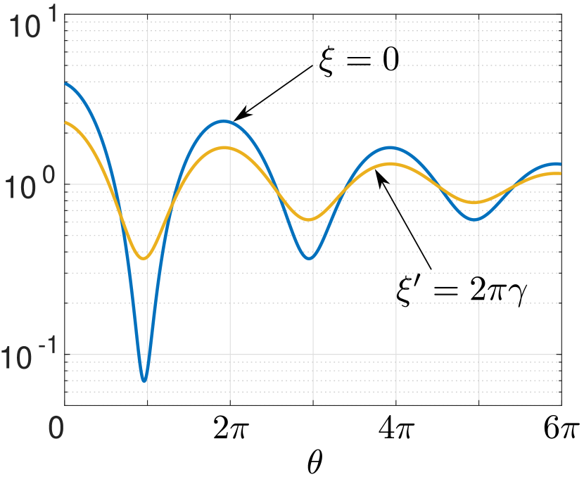
Figure 2: The potential $U_{\xi}(\theta)$ (blue) and its “sibling” $U_{\xi^{\prime}}(\theta)$ (brown curve), with $\xi^{\prime}=\xi+2\pi\gamma$. (In this plot, $\gamma=\frac{1}{10}$, $\xi=0$, and $\xi^{\prime}=\frac{2}{10}\pi$.) The function $U_{\xi^{\prime}}(\theta)$ is obtained from $U_{\xi}(\theta)$ by the $2\pi$ horizontal translation of the latter.

Taking advantage of the symmetry

$$U_{\xi}(\theta+2\pi)=U_{\xi+2\pi\gamma}(\theta),$$ (34)

we can extend our analysis beyond the interval $[0,2\pi)$. Assuming $\xi>\xi_{c}$, the potential $U_{\xi}(\theta)$ has a pair of extrema in each interval $[2\pi\ell,2\pi(\ell+1))$ with $\ell=1,2,...$. The minimum is at

$$\theta^{(2\ell+1)}(\xi)=\theta^{(2\ell-1)}(\xi+2\pi\gamma)+2\pi$$

and the maximum at

$$\theta^{(2\ell+2)}(\xi)=\theta^{(2\ell)}(\xi+2\pi\gamma)+2\pi.$$ (35)

The value of the potential $U_{\xi}$ at its minimum $\theta^{(2\ell+1)}$ is equal to the value of the potential $U_{\xi+2\pi\gamma}$ at its own local minimum in the interval $[2\pi(\ell-1),2\pi\ell)$. (See Fig 2.) A similar rule governs the local maxima:

$$U_{\xi}(\theta^{(2\ell+2)}(\xi))=U_{\xi+2\pi\gamma}(\theta^{(2\ell)}(\xi+2\pi\gamma)).$$ (36)

As the parameter $\xi$ is increased, the value of the potential $U_{\xi}$ at its maximum in $[0,2\pi)$ decreases:

$$\frac{\mathrm{d}}{\mathrm{d}\xi}U_{\xi}(\theta^{(2)}(\xi))=-\frac{2\sin(\theta^{(2)}+\beta)\sin(\theta^{(2)}+2\beta)}{\gamma^{2}\sqrt{1+\gamma^{2}}}<0.$$

Here we took into account (28) and (33). We also note that according to (27), the point $\theta^{(1)}(\xi)$ approaches $\pi-2\beta$ and $\theta^{(2)}(\xi)$ approaches $2\pi-2\beta$ as $\xi\to\infty$. Hence, by equation (29) the maximum value of the potential in the interval $[0,2\pi)$ is bounded from below:

$$U_{\xi}(\theta^{(2)}(\xi))>\frac{1}{1+\gamma^{2}}.$$ (37)

Finally, the inequality (28) implies

$$\cos(\theta^{(2)}+\beta)<\cos\beta.$$ (38)

Making use of (38) one can establish the following relation, valid for all $\xi$:

$$U_{\xi}(0)>U_{\xi}(\theta^{(2)}(\xi)).$$

The symmetry identities (34), (35) and (36) yield the inequality

$$U_{\xi}(2\pi)>U_{\xi}(\theta^{(4)}(\xi)).$$ (39)

III.4 Spin trajectories from particle flight paths

Consider a trajectory of the spin system (17) passing through a point on the equator ($Z=0$) at time $\tau=0$. The corresponding fictitious particle starts its motion from rest ($\dot{\theta}(0)=0$), with the values of integrals $\xi$ and $\mathcal{R}$ defined by the initial data, $\theta_{0}$ and $\eta(0)$:

$$\xi=\eta(0)-\gamma(\theta_{0}+\beta),\quad{\mathcal{R}}=\sqrt{U_{\xi}(\theta_{0})}.$$

The implicit solution $\tau(\theta)$ of equation (24) is given by the integral

$$\tau=\pm\int_{\theta_{0}}^{\theta}\frac{d\theta^{\prime}}{\sqrt{{\mathcal{R}}^{2}-U_{\xi}(\theta^{\prime})}}.$$ (40)

The solution is valid for all $\theta$ such that the expression under the radical is positive in the interval $(\theta_{0},\theta)$. Without loss of generality we may let $\theta_{0}$ lie in the interval $[0,2\pi)$.

If $\partial U_{\xi}/\partial\theta<0$ at $\theta=\theta_{0}$, the $\theta$-particle will start moving in the positive direction and we choose the positive sign in (40). The corresponding spin trajectory ${\bf S}(\tau)$ will emerge into the northern hemisphere. If $\partial U_{\xi}/\partial\theta>0$ at $\theta=\theta_{0}$, the particle will start moving in the negative direction and we choose the negative sign in (40). In that case, the point ${\bf S}$ will move into the southern hemisphere.

The negative-time motions can be classified in a similar manner.

For a given value of $\gamma$, the character of motion is determined by the values of the parameters $\mathcal{R}$ and $\xi$. Since two or three values of $\theta_{0}\in[0,2\pi)$ can be mapped to the same $U_{\xi}$, we also need to indicate the position of $\theta_{0}$ relative to the minimum and maximum of $U_{\xi}(\theta)$.

(a) Assume first that $\mathcal{R}>\gamma^{-1}$. If $\xi>\xi_{c}$, the potential $U_{\xi}(\theta)$ has a sequence of local maxima at $\theta^{(2\ell)}$, $\ell=1,2,...$, while if $\xi_{c}-2\pi\gamma m<\xi<\xi_{c}-2\pi\gamma(m-1)$ ($m=1,2,...$), the potential is monotonically decreasing in $(-\infty,2\pi m)$ but has local maxima in each interval $[2\pi\ell,2\pi(\ell+1))$ with $\ell=m,m+1,...$. In either case, all local maxima $U_{\xi}(\theta^{(2\ell)})$ lie below $\gamma^{-2}$ (cf. (29)). Consequently, the particle will accelerate to some positive speed and then continue moving with an oscillatory positive velocity bounded from below: $\dot{\theta}>\sqrt{{\mathcal{R}}^{2}-\gamma^{-2}}$. Regardless of $\xi$, the particle will eventually escape to infinity: $\theta\to\infty$, with $\eta\to\infty$ as well. A similar asymptotic behaviour occurs in the negative-time domain: $\eta\to\infty$ as $\tau\to-\infty$.

The implicit solution (40) with $\eta\to\infty$ as $\tau\to\pm\infty$ admits a simple interpretation in terms of the spin components (18). (The corresponding trajectories on the spin sphere have been numerically delineated in Ref Graefe .) Similar to the system (4) (Fig 1 (a)) the sphere with $\mathcal{R}>\gamma^{-1}$ supports a pair of latitudinal fixed points, with

$$X=\frac{1}{1+\gamma^{2}},\quad Y=-\gamma X,\quad Z=\pm\sqrt{{\mathcal{R}}^{2}-X}.$$ (41)

The fictitious particle’s journeys from infinity to $\theta_{0}$ and back to infinity correspond to trajectories ${\bf S}(\tau)$ emerging from the unstable focus in the southern hemisphere and spiralling into the attractor in the north (Fig 3(a)).

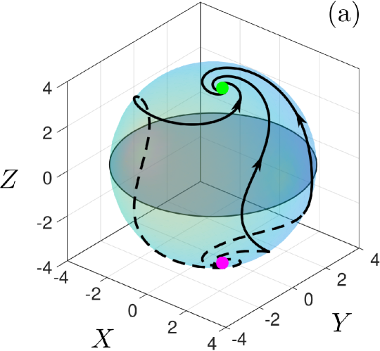
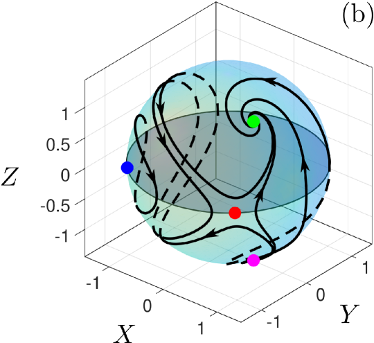
Figure 3: Trajectories of the system (17) on the surface of the sphere of the radius $\mathcal{R}>\gamma^{-1}$ (a) and $(1+\gamma^{2})^{-1/2}<\mathcal{R}<\gamma^{-1}$ (b). In this and the next figure, $\gamma=\frac{1}{2}$.

(b) The next range to consider is $(1+\gamma^{2})^{-1/2}<\mathcal{R}<\gamma^{-1}$. Let the function $\xi_{d}(\mathcal{R})$ be defined as the inverse of the monotonically decreasing function ${\mathcal{R}}=\sqrt{U_{\xi}(\theta^{(2)}(\xi))}$. In view of (30), $\xi_{d}(\mathcal{R})>\xi_{c}$ for all $\mathcal{R}$ in the current range. As $\mathcal{R}$ approaches $\gamma^{-1}$ from below, the value $\xi_{d}(\mathcal{R})$ approaches $\xi_{c}$; as $\mathcal{R}$ approaches $(1+\gamma^{2})^{-1/2}$ from above, we have $\xi_{d}\to\infty$.

When $\xi<\xi_{c}$ or $\xi>\xi_{d}(\mathcal{R})$, the total energy ${\mathcal{R}}^{2}$ of the particle is greater than $U_{\xi}$ at all of its local maxima. Accordingly, the particle escapes to infinity as $\tau\to\pm\infty$. This class of motions corresponds to the heteroclinic trajectories on the sphere flowing from the southern to the northern focus in (41) (Fig 3 (b)).

Turning to the interval $\xi_{c}<\xi<\xi_{d}$ we first assume that the point $\theta_{0}$ lies to the left of the local maximum $\theta^{(2)}$. In that case the energy of the $\theta$-particle is insufficient to overcome the potential barrier: ${\mathcal{R}}^{2}<U_{\xi}(\theta^{(2)}(\xi))$. The particle becomes trapped in the potential well, and its motion is periodic with period

$$T=\left|\int_{\theta_{0}}^{\theta_{\mathrm{turn}}}\frac{d\theta^{\prime}}{\sqrt{{\mathcal{R}}^{2}-U_{\xi}(\theta^{\prime})}}\right|.$$

Here $\theta_{\mathrm{turn}}$ is the second root of the equation ${\mathcal{R}}^{2}=U_{\xi}(\theta)$ to the left of the maximum of the potential in the interval $[0,2\pi)$.

To interpret the periodic motions in terms of trajectories on the sphere, we note that as $\mathcal{R}$ is decreased through $\gamma^{-1}$, a saddle-centre bifurcation brings about two new fixed points lying on the equator:

$$X=\pm\mathcal{R}\sqrt{1-\gamma^{2}{\mathcal{R}}^{2}},\quad Y=-\gamma{\mathcal{R}}^{2},\quad Z=0.$$ (42)

For $\mathcal{R}$ in the interval $(1+\gamma^{2})^{-1/2}<\mathcal{R}<\gamma^{-1}$, the point with negative $X$ is a centre and the one with positive $X$ is a saddle. The oscillations of the $\theta$-particle in the potential well translate into a thicket of closed orbits surrounding the centre (Fig 3(b)).

If the point $\theta_{0}$ lies to the right of the local maximum $\theta^{(2)}$ (that is, if $\theta^{(2)}<\theta_{0}<2\pi$), the particle will escape to infinity: $\theta\to\infty$ as $\tau\to\infty$. It cannot be captured by the potential well in the interval $[2\pi,4\pi)$ because $U_{\xi}(\theta_{0})$ is greater than $U_{\xi}(2\pi)$ and therefore, by inequality (39), greater than the potential barrier $U_{\xi}(\theta^{(4)}(\xi))$.

By examining the neighbourhood of the saddle point in Fig 3(b)), one can readily reconstruct a homoclinic curve connecting the saddle to itself. This trajectory results by choosing $\xi=\xi_{d}(\mathcal{R})$. The homoclinic curve separates the family of closed orbits from the focus-to-focus flows.

(c) Finally, it remains to examine the range $\mathcal{R}<(1+\gamma^{2})^{-1/2}$. Since the function $U_{\xi}(\theta)$ with $\xi<\xi_{c}$ is monotonically decreasing in $[0,2\pi)$, and since $U_{\xi}(2\pi)>(1+\gamma^{2})^{-1}$ by equation (25a), this parameter range is only accessible to initial conditions with $\xi>\xi_{c}$. In view of (37), the $\theta$-particle with $\dot{\theta}(0)=0$ and $\theta_{0}$ satisfying $U_{\xi}(\theta_{0})={\mathcal{R}}^{2}$ finds itself trapped in a potential well.

The disappearance of aperiodic solutions $\theta(\tau)$ is consistent with the bifurcation occurring as $\mathcal{R}$ is reduced below $(1+\gamma^{2})^{-1/2}$. At this value of $\mathcal{R}$, the pair of latitudinal fixed points (41) merges with the saddle on the equator forming the second centre (Fig 4(a)). The two centre points are given by equations (42); each point is surrounded by a family of closed orbits (Fig 4 (b)). The closed orbits are described by periodic motions of the particle in the potential well.

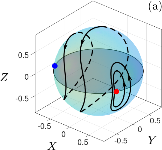
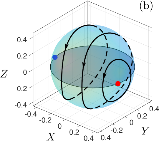
Figure 4: Trajectories of the system (17) on the surface of the sphere of the radius $\mathcal{R}=\frac{1}{\sqrt{1+\gamma^{2}}}$ (a) and $\mathcal{R}<\frac{1}{\sqrt{1+\gamma^{2}}}$ (b).

IV Integrable $\mathcal{PT}$-symmetric necklaces

In a nonhermitian necklace of more than two waveguides, the trapping of trajectories in a finite part of the phase space may require each site to coordinate its gain and loss rate with both of its left and right neighbours. This cross-compensation mechanism is more subtle than the cross-stimulation of two channels of a dimer. In this section, we exemplify the cross-compensation with arrays consisting of three and four elements.

IV.1 Trimer

We identified several $\mathcal{PT}$-symmetric trimers endowed with a Hamiltonian structure and possessing an integral of motion that prevents the blow-up behaviour. However, only one of these models has three first integrals in involution and defines a Liouville-integrable dynamical system.

The trimer in question is a nonhermitian extension of the closed Ablowitz-Ladik chain:

$$iu_{t} =(1+|u|^{2})(v+w)(1+i\gamma),$$ (43a)

$$iv_{t} =(1+|v|^{2})\left[u+w+i\gamma(w-u)\right],$$ (43b)

$$iw_{t} =(1+|w|^{2})(u+v)(1-i\gamma).$$ (43c)

The system is invariant under the product of the $\mathcal{P}$ and $\mathcal{T}$ transformations, where

$$\mathcal{P}u(t)=w(t),\quad\mathcal{P}v(t)=v(t),\quad\mathcal{P}w(t)=u(t)$$

and

$$\mathcal{T}u(t)=u^{*}(-t),\quad\mathcal{T}v(t)=v^{*}(-t),\quad\mathcal{T}w(t)=w^{*}(-t).$$

Similar to the dimers (2) and (16), the linearisation of equations (43) about $u=v=w=0$ gives a system with a hermitian matrix and a purely real spectrum. Accordingly, the trimer (43) does not suffer the linearised $\mathcal{PT}$-symmetry breaking as the value of $\gamma$ is raised.

The system (43) admits a canonical representation

$$u_{t}=\{H,u\},\quad v_{t}=\{H,v\},\quad w_{t}=\{H,w\}$$

with the Hamilton function

$$H=(1+i\gamma)({u^{*}}v+{v^{*}}w+w{u^{*}})+\text{c.c.}$$ (44)

and the Gerdjikov-Ivanov-Kulish (GIK) bracket GIK . Here

$$\{u,{u^{*}}\}=i(1+|u|^{2}),\quad\{v,{v^{*}}\}=i(1+|v|^{2}),$$

$$\{w,{w^{*}}\}=i(1+|w|^{2}),$$

while all other brackets are equal to zero: $\{u,v\}=\{u,v^{*}\}=...=0$.

In addition to the Hamiltonian, the system conserves the total momentum,

$$M=(\gamma-i)({u^{*}}v+{v^{*}}w-w{u^{*}})+\text{c.c.},$$

and a product

$$\Pi=(1+|u|^{2})(1+|v|^{2})(1+|w|^{2}).$$

The integrals $M$ and $\Pi$ commute: $\{M,\Pi\}=0$. Consequently, the system (43) is completely integrable.

Note that since the total power $P=|u|^{2}+|v|^{2}+|w|^{2}$ is bounded from above by the conserved quantity $\Pi$, the trimer does not exhibit any unbounded trajectories.

It is worth noting that the absence of blow-up regimes is not related to the integrability of the model but is instead a consequence of the compensation of gain and loss rate in the neighbouring channels. This can be illustrated by the following family of nonintegrable cross-compensated trimers:

$$iu_{t} =f_{1}(|u|^{2})(v+w)(1+i\gamma),$$ (45a)

$$iv_{t} =f_{2}(|v|^{2})\left[u+w+i\gamma(w-u)\right],$$ (45b)

$$iw_{t} =f_{3}(|w|^{2})(u+v)(1-i\gamma).$$ (45c)

In equations (45), $f_{n}(\rho)$ ($n=1,2,3$) are positive functions with $f_{n}(0)=1$ and $f_{n}(\rho)\leq 1$ for $\rho>0$. The model (45) is Hamiltonian with the Hamilton function (44) and obvious modification of the bracket. It has the first integral

$$I=F_{1}(|u|^{2})+F_{2}(|v|^{2})+F_{3}(|w|^{2}),$$

where

$$F_{n}(\rho)=\int_{0}^{\rho}\frac{d\rho^{\prime}}{f_{n}(\rho^{\prime})}.$$

Since $F_{n}(\rho)\geq\rho$, the total power is bounded from above by $I$ and no trajectory can escape to infinity.

IV.2 Quadrimer

Guided by the symplectic structure and cross-compensating arrangement of the integrable $\mathcal{PT}$-symmetric trimer, it is not difficult to construct a four-waveguide necklace with similar properties:

$$i\dot{u}_{1} =(1+|u_{1}|^{2})(u_{2}+u_{4})(1+i\gamma),$$ (46a)

$$i\dot{u}_{2} =(1+|u_{2}|^{2})\left[u_{3}+u_{1}+i\gamma(u_{3}-u_{1})\right],$$ (46b)

$$i\dot{u}_{3} =(1+|u_{3}|^{2})\left[u_{4}+u_{2}+i\gamma(u_{4}-u_{2})\right],$$ (46c)

$$i\dot{u}_{4} =(1+|u_{4}|^{2})(u_{1}+u_{3})(1-i\gamma).$$ (46d)

The quadrimer (46) is $\mathcal{PT}$-symmetric, with the $\mathcal{P}$ operator defined by

$$\mathcal{P}u_{1}(t)=u_{4}(t),\quad\mathcal{P}u_{2}(t)=u_{3}(t),$$

$$\mathcal{P}u_{3}(t)=u_{2}(t),\quad\mathcal{P}u_{4}(t)=u_{1}(t),$$

and $\mathcal{T}$ as in $\mathcal{T}u_{n}(t)=u_{n}^{*}(-t)$. The linearisation of the quadrimer (46) about $u_{1}=u_{2}=u_{3}=u_{4}=0$ gives a system with a hermitian matrix and a purely real spectrum.

The quadrimer retains a similar canonical representation to the trimer (43), with the Hamiltonian

$$H=(1+i\gamma)({u_{1}^{*}}u_{2}+{u_{2}^{*}}u_{3}+{u_{3}^{*}}u_{4}+u_{4}{u_{1}^{*}})+\text{c.c.}$$ (47)

and GIK bracket. Here

$$\{u_{n},{u_{m}^{*}}\}=i(1+|u_{n}|^{2})\delta_{nm},$$

$$\{u_{n},{u_{m}}\}=0,\quad\{u_{n}^{*},{u_{m}}^{*}\}=0.$$

In direct analogy to the trimer, the system conserves the total momentum

$$M=(\gamma-i)({u_{1}^{*}}u_{2}+{u_{2}^{*}}u_{3}+{u_{3}^{*}}u_{4}-u_{4}u_{1}^{*})+\text{c.c.},$$

as well as the product

$$\Pi=\prod_{n=1}^{4}(1+|u_{n}|^{2}).$$

In addition, the quadrimer conserves a quartic quantity

$$I=(1-i\gamma)(u_{1}u_{2}^{*}u_{3}u_{4}^{*}-u_{2}u_{4}^{*}-u_{1}u_{3}^{*})+c.c.$$ (48)

All four integrals $H$, $M$, $\Pi$ and $I$ mutually commute, and consequently the system (46) is completely integrable.

V Concluding remarks

In this paper, we explored a class of the $\mathcal{PT}$-symmetric discrete Schrödinger equations with purely-nonlinear nonhermitian terms. An a priori advantage of systems of this type in physics is that the trivial solution remains stable and linearised $\mathcal{PT}$-symmetry unbroken regardless of the value of the gain-loss coefficient.

We have identified two nonequivalent dimers that, in addition to preserving the linearised $\mathcal{PT}$-symmetry, conserve the quantity $|u|^{2}+|v|^{2}$. (In the optical context, this means that the total power of light is conserved.) The power conservation is brought about by the cross-stimulation of the two channels of the dimer. The constancy of $|u|^{2}+|v|^{2}$ ensures that no trajectories of these dynamical systems escape to infinity.

Remarkably, both dimers possess a canonical structure and a first integral independent of the Hamiltonian. This establishes the Liouville integrability of the two systems. The transformation to the canonical variables allowed us to construct their general analytical solution.

The cross-compensation of the gain and loss rate in the neighbouring channels remains an efficient blow-up prevention mechanism in the case of the nonhermitian Schrödinger necklaces — the ring-shaped arrays of $N$ waveguides necklaces . We have exemplified this idea with the construction of a family of trimers ($N=3$) whose trajectories are confined to a finite part of their phase space. The entire family is endowed with a canonical structure while one member of the family has 3 first integrals in involution and defines a completely integrable system.

Finally, we have identified a completely integrable cross-compensated quadrimer — a $\mathcal{PT}$-symmetric necklace of $N=4$ waveguides.

- (1) C M Bender and S Boettcher, Phys Rev Lett 80 5243 (1998)
- (2) C M Bender, PT Symmetry in Quantum and Classical Physics. World Scientific (2018)
- (3) V V Konotop, J Yang, D A Zezyulin 2016 Rev Mod Phys 88 035002; S V Suchkov, A A Sukhorukov, J Huang, S V Dmitriev, C Lee, Y S Kivshar 2016 Laser and Photonics Reviews 10 177; S Longhi 2017 EPL 120 64001; Parity-time Symmetry and Its Applications. D Christodoulides and J Yang (editors). Springer Tracts in Modern Physics 280 (2018); R El-Ganainy, K Makris, M Khajavikhan, ZH Musslimani, S Rotter and D N Christodoulides 2018 Nature Phys 14 11; H Zhao, L Feng 2018 National Science Review 5 183; ŞK Özdemir, S Rotter, F Nori and L Yang 2019 Nat. Mater. 18 783
- (4) I V Barashenkov, D E Pelinovsky and P Dubard 2015 Journ Phys A Math Theor 48 325201;
- (5) I V Barashenkov, M Gianfreda 2014 J. Phys. A: Math. Theor. 47 282001; A Khare and A Saxena 2017 J. Phys. A: Math. Theor. 50 055202
- (6) I V Barashenkov 2014 Phys Rev A 90 045802
- (7) J Cuevas–Maraver, A Khare, P G Kevrekidis, H Xu, A Saxena 2015 Int Journ Theor Phys 54 3960; H Xu, P G Kevrekidis and A Saxena 2015 J Phys A: Math Theor 48 055101; X Li and Z Yan 2017 Chaos 27 013105
- (8) P G Kevrekidis, D E Pelinovsky and D Y Tyugin 2013 J. Phys. A: Math. Theor. 46 365201; J Pickton and H Susanto 2013 Phys. Rev. A 88 063840
- (9) I V Barashenkov, G S Jackson, S Flach 2013 Phys Rev A 88 053817
- (10) H Ramezani, T Kottos, R El-Ganainy and D N Christodoulides 2010 Phys. Rev. A 82 043803; A A Sukhorukov, Z Xu and Y S Kivshar 2010 Phys. Rev. A 82 043818; A S Rodrigues, K Li, V Achilleos, P G Kevrekidis, D J Frantzeskakis and C M Bender 2013 Rom. Rep. Phys. 65 5
- (11) R. El-Ganainy, K. G. Makris, D. N. Christodoulides, and Z. H. Musslimani 2007 Opt Lett 32 2632; C E Rüter, K G Makris, R El-Ganainy, D N Christodoulides, M Segev and D Kip 2010 Nat. Phys. 6 192; C Milian, Y V Kartashov, D V Skryabin, L Torner 2018 Opt Lett 43 979; V B de la Perriére, Q Gaimard, H Benisty, A Ramdane, A Lupu 2019 J. Phys. D: Appl. Phys. 52 255103; S K Gupta, Y Zou, X-Y Zhu, M-H Lu, L-J Zhang, X-P Liu and Y-F Chen 2020 Adv. Mater. 32 1903639; J Song, F Yang, Z Guo, X Wu, K Zhu, J Jiang, Y Sun, Y Li , H Jiang, and H Chen 2021 Phys Rev Applied 15 014009
- (12) A. U. Hassan, H. Hodaei, M.-A. Miri, M. Khajavikhan, and D.N. Christoudoulides 2015 Phys. Rev.A 92, 063807
- (13) E M Graefe, H J Korsch, A E Niederle 2008 Phys. Rev. Lett. 101 150408; E M Graefe, H J Korsch, A E Niederle 2010 Phys. Rev. A 82, 013629; E M Graefe 2012 J. Phys. A: Math. Theor. 45 444015
- (14) W D Heiss, H Cartarius, G Wunner and J Main 2013 J. Phys. A: Math. Theor. 46 275307; I Chestnov, Y G Rubo, A Nalitov and A Kavokin 2021 Phys Rev Research 3 033187; Y-P Wu, G-Q Zhang, C-X Zhang, J Xu, D-W Zhang 2022 Frontiers of Phys 17 42503
- (15) H. Benisty, A. Degiron, A. Lupu, A. De Lustrac, S. Chénais, S. Forget, M. Besbes, G. Barbillon, A. Bruyant, S. Blaize, G. Lérondel 2011 Opt. Express 19 18004; V Klimov and A Lupu 2019 Phys Rev B 100 245434; S Sanders and A Manjavacas 2020 Nanophotonics 9 473; J Chen and Y Fan 2022 Optics Communications 505 127530; X Chen, H Wang, J Li, K Wong and D Lei 2022 Nanophotonics 11 2159;
- (16) I V Barashenkov and A Chernyavsky 2020 Physica D 409 132481
- (17) J. Schindler, Z. Lin, J.M. Lee, H. Ramezani, F.M. Ellis, T. Kottos 2012 J. Phys. A 45 444029; H. Ramezani, J. Schindler, F.M. Ellis, U. Gunther, T. Kottos 2012 Phys. Rev. A 85 062122; S Assawaworrarit, X Yu and S Fan 2017 Nature 546 387; M Chitsazi, H Li, F M Ellis, and T Kottos 2017 Phys Rev Lett 119 093901; W Cao, C Wang, W Chen, S Hu, H Wang, L Yang and X Zhang 2022 Nature Nanotechnology 17 262; R Kononchuk, J Cai, F Ellis, R Thevamaran and T Kottos 2022 Nature 607 697
- (18) A. E. Miroshnichenko, B. A. Malomed, and Yu. S. Kivshar 2011 Phys. Rev. A 84 012123; A. U. Hassan, H. Hodaei, M.-A. Miri, M. Khajavikhan, and D.N. Christoudoulides 2016 Phys. Rev. E 93 042219; J R Parkavi and V K Chandrasekar 2020 J. Phys. A: Math. Theor. 53 195701
- (19) S. Karthiga, V. K. Chandrasekar, M. Senthilvelan and M. Lakshmanan 2017 Phys. Rev. A 95 033829
- (20) J D Huerta Morales, B M Rodriguez-Lara, and B A Malomed 2017 Opt. Lett. 42 4402; J D Huerta Morales 2018 Opt. Comm. 424 44
- (21) K Li, P G Kevrekidis, D J Frantzeskakis, C E Rüter and D Kip 2013 J. Phys. A: Math. Theor. 46 375304; M. Duanmu, K. Li, R. L. Horne, P. G. Kevrekidis and N. Whitaker 2013 Phil Trans R Soc A 371 20120171; S V Suchkov, F Fotsa-Ngaffo, A Kenfack-Jiotsa, A D Tikeng, T C Kofane, Y S Kivshar and A A Sukhorukov 2016 New J. Phys. 18 065005; C A. Downing, D Zueco and L Martín-Moreno 2020 ACS Photonics 7 3401; V Le Duc, J K Kalaga, W Leoński, M Nowotarski, K Gruszka and M Kostrzewa 2021 Symmetry 13 2201
- (22) V S Gerdzhikov, M I Ivanov and P P Kulish 1980 JINR preprint E2-80-882; V S Gerdzhikov, M I Ivanov and P P Kulish 1984 Journ Math Phys 25 25
- (23) K Li and P G Kevrekidis 2011 Phys. Rev. E 83 066608; I V Barashenkov, L Baker, N V Alexeeva 2013 Phys Rev A 87 033819; P G Kevrekidis, D E Pelinovsky and D Y Tyugin 2013 SIAM J. Appl. Dyn. Syst. 12 1210; A J Martínez, M I Molina, S K Turitsyn and Y S Kivshar 2015 Phys. Rev. A 91 023822; C Castro-Castro, Y Shen, G Srinivasan, A B Aceves and P G Kevrekidis 2016 Journal of Nonlinear Optical Physics and Materials 25 1650042; J D Huerta Morales, J Guerrero, S López-Aguayo and B M Rodríguez-Lara 2016 Symmetry 8 83; I V Barashenkov and D Feinstein 2021 Phys Rev A 103 023532