Synchronized Rotations in Chemotactic Active Matter

Abstract

Many microorganisms use chemical ’signaling’ - a quintessential self-organizing strategy in non-equilibrium- that can induce spontaneous aggregation and coordination in behavior. This inspired us to construct a minimal model for a collection of active Brownian particles (ABPs) having soft repulsive interactions on a chemically-quenched patterned substrate. We numerically investigate the interplay between chemo-phoretic interactions and activity for a proposed variant of the Keller-Segel model for chemotaxis. Such competition not only results in a chemo-motility-induced phase-separated state but also a new cohesive phase with synchronized rotations, amongst two other dynamically nearly-frozen phases. Our results suggest that rotational order can emerge in systems by virtue of activity and repulsive interactions alone without an explicit alignment interaction.

I Introduction

Active matter refers to any collection of entities that individually and dissipatively break time-reversal symmetry and are innately out of equilibrium rmpbechinger2016 ; annalsofphys2005 ; vicsek2012 ; rmp2013 . The living world is overwhelmingly constituted by active matter in the form of cells cell , flocks of birds physicstoday2006 , human crowds humancrowd1 ; humancrowd2 , etc. Active units not only possess interesting features as a collection but also show intriguing individual dynamics and reach a statistical steady state in response to an external stimulus that is central to many fascinating behaviors in active systems, viz. collective foraging foraging , swarming of bacteria bacteria1 ; bacteria3 , dynamical clustering in active colloids activecolloids , etc. Several of these collective effects result from velocity alignment mechanisms.

Many studies have assumed that large-scale properties of the system only depend on the symmetry of interactions, as is expected for an equilibrium system. This may be true for unicellular organisms where physical interactions dominate over biological ones, but not in the case of larger organisms where interactions are the result of complex processes for sustenance. The response of agents to a stimulus - customarily modeled by field variations in density densityfield , chemical potential chemicalfield , polarization polfield ; pol2 - has finite effects on the spatiotemporal self-propulsion speeds of the agents that often leads to long-range anisotropic interactions. The effect of quenched (time-independent) disorder/stimulus in the dynamical phases of self-propelled particles coldperuani ; vivekepje ; patternedBech ; quench is a topic of great interest but is lacking in its representation in literature.

With the rapid development of synthetic microswimmers, it has become easier to employ synthetic signaling as a design principle to create and study pattern formations acc1 ; acc2 ; activerotors . For example, the response of active agents to a chemo-phoretic field and its effect on the non-equilibrium phenomena unique to active systems, motility-induced phase separation (MIPS) arXiv and chemotactic stabilization of hydrodynamic instabilities in active suspensions instability has been studied. Furthermore, the interplay between steric, chemo-phoretic interactions and activity, leads to the emergence of a phase-separated state very recently coined as the chemo-motility-induced phase-separated (CMIPS) state softmatter2023 . On the other hand, the effect of surface interactions and morphology on motility can be riveting bact_morph . The motion of a Brownian particle as it flows through periodically modulated potential-energy landscapes in two dimensions experiences a crossover from free-flowing to locked-in transport that depends on the periodicity of the landscape morphology . A self-propelled colloid faces a competition between hindered diffusion from the trapping potential on a periodic crystalline surface and enhanced diffusion due to active motion periodicsurface . Further, a periodic arrangement of obstacles on the substrate is found to enhance the persistent motion of an ABP and induce directionality in its motion sudipta .

Such studies motivated us to pursue a quench disorder framework for a collection of ABPs in a chemically patterned substrate. In this work, we achieve the same by exposing the well-studied collective ABP problem softmatterpritha2018 ; prl2012filly to the Keller-Segel KS1 -KS2 model of chemotaxis (swimming up chemical gradients). The interplay between chemo-phoretic interactions and activity suppresses the dynamical phases that a quench-free ABP problem would otherwise produce. In addition to obtaining a CMIPS state, a hopping transport phase, and a localized phase, we obtain a non-trivial dynamical phase with synchronized rotations. The emergence of such a phase is accompanied by a cooperative balance between the active force and the chemical force.

The remainder of the article is organized as follows. In section II, we discuss the model for chemotaxis and numerical details for the Brownian simulations. In section III, we present the single-particle model and the interacting model. The state diagram as a function of activity and steepness of the chemical gradient, the steady-state structural behavior, the dynamical characteristics of the phases, and the phase transition are described for the latter case. We summarize our major findings in section IV and suggest directions for future work.

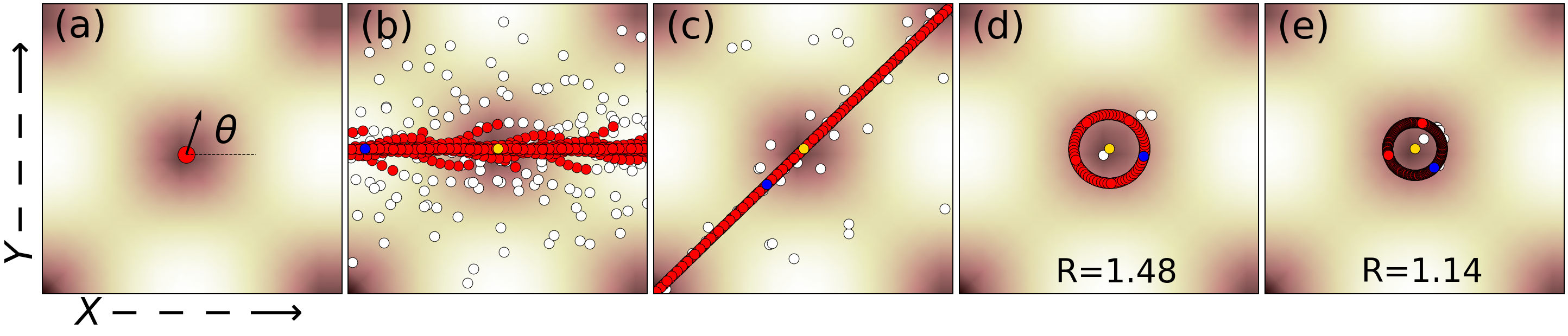
Figure 1: (a) Schematic of the single-particle model for L=$\lambda$/2. Background color code: white for high $\nabla$c, brown for low $\nabla$c. $\theta$ is the orientation of the particle. Arrowhead shows the velocity direction and the arrow length corresponds to speed. (b-e) Position of a single particle is shown for all times in a simulation run for system configurations $\nu=5$ and (b) $\epsilon=0.001$ (c) $\epsilon=0.005$ (d) $\epsilon=0.03$ (e) $\epsilon=0.01$. R is the radius of circular motion. Particle color code: white: simulation time t$<$250$\tau_{c}$, red: simulation time $250\tau_{c}<t<1000\tau_{c}$, yellow: initial position, blue: final position.

II Model and Numerical details

A collection of ABPs with radii $a_{0}$ having a self-propulsion speed $v_{0}$ are simulated on a two-dimensional surface with a patterned chemical concentration. The steric force $\textbf{F}_{ij}$ between two disks i and j is short-ranged and repulsive: $\textbf{F}_{ij}=-k(2a_{0}-r_{ij})\hat{\textbf{r}}_{ij}$, if $r_{ij}<2a_{0}$ and $\textbf{F}_{ij}=\textbf{0}$ otherwise. Here, $\textbf{r}_{ij}=\textbf{r}_{j}-\textbf{r}_{i}$. In addition to the steric repulsion, particles also experience a time-invariant periodic chemical concentration on the substrate: $c(\textbf{r})=h_{0}sin(\frac{2\pi x}{\lambda})sin(\frac{2\pi y}{\lambda})$ with wavelength $\lambda$ chosen to be $25a_{0}$ and amplitude $h_{0}$ is varied. For a particular $h_{0}$, each local minima of the patterned $c({\bf r})$ can be treated as a separate subsystem containing a sufficient number of ABPs. Due to the chemical field, particles experience both a force acting on their center of mass and a torque due to the local gradient of the chemical field. Then, the motion of a chemotactic particle self-propelling with a velocity $v_{0}$ (independent of chemotaxis) in a direction p(t) = $(cos\theta_{i}(t),sin\theta_{i}(t))$ is given by the following over-damped equations :

$$\partial_{t}\textbf{r}_{i}=v_{0}\textbf{p}_{i}(t)+\beta_{D}\nabla c(\textbf{r}_{i},t)+\mu\sum_{j\neq i}\textbf{F}_{ij}$$ (1)

$$\partial_{t}\textbf{$\theta$}_{i}=\beta\textbf{p}_{i}(t)\times\nabla c(\textbf{r}_{i},t)+\eta^{R}_{i}(t)$$ (2)

Equations 1 and 2 model the response of active particles to the local chemical gradient drawing from the Keller-Segel (KS) model of chemotaxis. $\beta_{D}$ is the chemotactic coupling coefficient which measures the translational diffusion in response to the chemical gradient. Angular diffusion is measured by the orientational coupling coefficient $\beta$. The swimming direction of the particle is chemo-attractive if $\beta_{D},\beta>0$ (motion towards the chemical gradient) and chemo-repulsive if $\beta_{D},\beta<0$ (motion away from the chemical gradient) for the position and orientation respectively. We fix $\beta_{D}=\beta=1$. The symmetry in the functional form of c(r) ensures that the same dynamical steady-states are reached in our system for both chemo-attractive and chemo-repulsive interactions.

The ratio of translational diffusion to angular diffusion due to the chemical concentration sets an intrinsic time scale: $\tau_{c}=\beta_{D}/\beta^{2}=1$. The ratio $\beta_{D}/\beta$ sets an intrinsic length scale: l_c, the length up to which a particle translates before it experiences a rotation due to the chemical gradient. All other times and lengths in the system are scaled with $\tau_{c}$ and $l_{c}$. The elastic time scale $(\mu k)^{-1}$ is fixed to $5\times 10^{-2}\tau_{c}$. $\eta^{R}_{i}(t)$ is the Gaussian white noise for thermal rotational diffusion with zero mean and delta correlation having the strength $D_{R}$. To compare the active force to the chemical force, we define a dimensionless activity $\nu=\frac{v_{0}}{\sqrt{\lambda^{-1}\beta_{D}\beta}}$ which is varied between $[0.25,10]$ as $v_{0}$ $\in[0.05,2]$. The surface gradient $\epsilon$ = $h_{0}/\lambda$ quantifies the steepness of chemical concentration and is kept in the range $[10^{-3},10^{1}]$. The dynamics and steady state of the system are studied by varying $\epsilon$ and $\nu$. Each realization of the system is $5\times$$10^{5}$ time steps long with a time step $\Delta t=5\times$$10^{-3}\tau_{c}$. All statistical quantities are recorded every $10^{3}$ steps. The system is studied for a $L\times L$ square geometry and the periodic boundary condition (PBC) is applied in both directions. For the purpose of statistical averaging, data from $20$ independent realizations are used.

III Results

III.1 Non-interacting model

We first study the effect of the patterned surface on the dynamics of a single particle by setting $\mu=0$ in Eq. 1 and $D_{R}=0$. A unit cell ($L=\lambda/2$) of the periodic chemical patterned substrate is chosen. A model cartoon is shown in Fig. 1 (a) and the trajectories for some system configurations are reported in Figs. 1 (b-e).

For low $\epsilon$ [see Fig. 1 (b-c)], the particle exhibits unconfined diffusive dynamics, the diffusivity reducing with increasing $\epsilon$. There is a preference to traverse along the $x-y$ direction followed by $x$ and $y$ directions owing to the form of c(r) and PBC. For moderate $\epsilon$, the particle is unable to escape the chemical valley where it was initialized [see Fig. 1 (d-e)]. However, sufficient $\nu$ can give the particle the required energy to deviate from the valley [refer to Appendix]. The combined effect results in the particle preferring to move tangentially to $\nabla$c minima. Note that the radius $R$ of circular motion decreases with increasing $\epsilon$ and increases with increasing $\nu$ [see annotations in Fig. 1 and Appendix]. For very high $\epsilon$, the confinement is strong and the particle is effectively localized, only to be freed by very high $\nu$.

III.2 Interacting model

We set $\mu=1$, $D_{R}=10^{-4}\tau_{c}^{-1}$ and $L=4\lambda$. The number of particles $\textit{N}\sim 2000$ in the system is decided by the packing fraction $\phi=\frac{N\times\pi a_{0}^{2}}{L\times L}$ which is fixed to $0.6$. The simulation starts from a homogeneous arrangement of particles with the same speeds and randomized orientations on the substrate. The chemical field dictates the particles to accumulate in regions where $\nabla$c is minimum. Consequently, periodic clusters form in systems in which $\epsilon$ is non-negligible. We explored the ($\nu$,$\epsilon$) phase-space and present the state diagram in Fig. 2. The characteristics of the obtained phases follow.

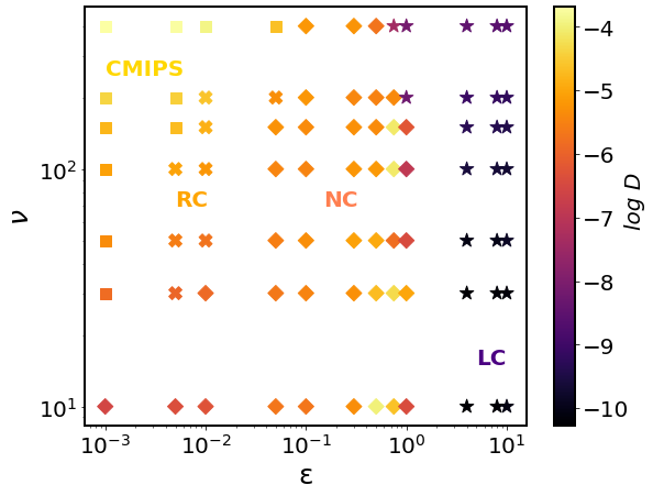
Figure 2: State diagram in the $(\nu,\epsilon)$ plane. Symbols correspond to phases: square for CMIPS, cross for RC, diamond for NC, star for LC. Colors are mapped to the strength of effective diffusivity D.

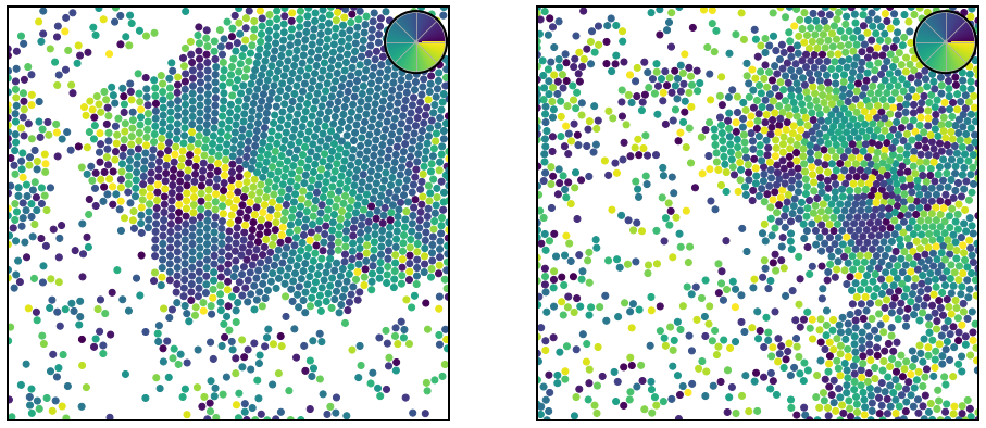
Figure 3: Late-time snapshots for two CMIPS systems: $\nu=5,\epsilon=0.001$ and $\nu=10,\epsilon=0.005$. Particles are colored according to their orientations as given by the color disc in the inset.

Chemo-motility-induced phase-separated (CMIPS) state: For very low $\epsilon\sim 10^{-3}$ and $\nu\geq 0.75$, we obtain a macroscopic cluster formation [see Fig. 3] wherein a dense liquid phase coexists with the gaseous phase. CMIPS is structurally similar to MIPS, but the origins of phase separation in CMIPS is due to an interplay between chemo-phoretic interactions that collapse particles into valleys of the chemical concentration forming clusters, and activity that disperses particles from the clusters. This is in contrast with the self-trapping positive feedback that leads to MIPS prl2012filly ; prl2013exp .

Rotating clusters (RC): For slightly higher $\epsilon\sim 10^{-2}$ and moderate $\nu$, the CMIPS phase is suppressed by chemotaxis. We obtain periodic clusters that rotate about their cluster centers [see Fig. 4 (a)] whose sense of rotation of a cluster may change with time [refer Supplementary Material $S2$]. Each cluster acts like a chemo-repulsive shell due to the local anisotropy in the chemical concentration. This constricts the freedom of a cluster to grow beyond a certain size.

Non-rotating clusters (NC): For higher $\epsilon\sim 10^{-1}$, field strength dominates highly over the activity. This results in the formation of connected periodic clusters [see Fig. 5 (a)] that allow hopping transport of particles between clusters to a considerable extent. These cluster boundaries lack curvature and possess sharp edges. They are also more closely packed than RC.

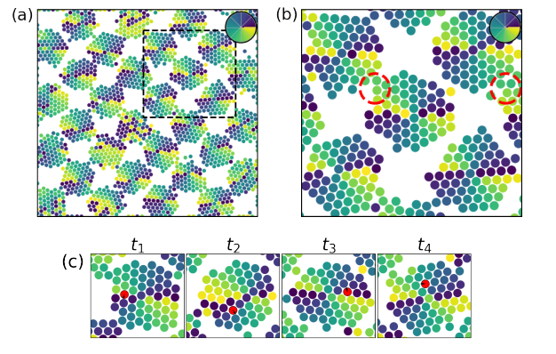
Figure 4: (a) Late-time snapshots for a RC system with $\nu=1.25,\epsilon=0.01$. (b) Zoomed-in snapshot of square-dashed area in (a). Red dashed circles indicate areas where particles are exchanged between clusters. (c) Position and velocity direction of a tagged particle (red) in a cluster for times $t_{1}<t_{2}<t_{3}<t_{4}$ separated by $20\tau_{c}$. Particles are colored according to their orientations as indicated by the color ring in the inset.

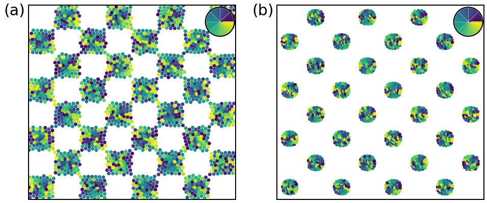
Figure 5: Late-time snapshots for (a) NC system with $\nu=5,\epsilon=1$ and (b) LC system with $\nu=5,\epsilon=10$. Particles are colored according to their orientations as indicated by the color ring in the inset.

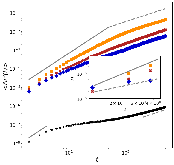
Figure 6: Mean-square displacement $<\Delta r^{2}>$ vs. time for the $4$ distinct phases. Inset shows diffusivity D as a function of $\nu$ for the first $3$ phases. The dashed line is drawn for slope $1$ and the solid line is drawn for slope $2$. Key: orange square for CMIPS $(\nu,\epsilon)=(3.75,0.001)$, red cross for RC $(2.5,0.01)$, blue diamond for NC $(3.75,0.1)$, and black star for LC $(3.75,5)$.

Localized clusters (LC): For very high $\epsilon\geq 10^{0}$, the clusters are completely localized and show little to no dynamics [see Fig. 5 (b)]. Particle trajectories asymptotically converge to bounded areas in space leading to trapping in the valleys of the chemical concentration. Cluster boundaries of LC are very sharp and the dynamics of one cluster are independent of the others in the system. Hence system collapses to the non-interacting model, i.e., each localized cluster can be treated as an independent subsystem.
We quantify the dynamics of the phases by calculating the mean square displacement (MSD) of the particles:

$$<\Delta r^{2}(t)>=<\frac{1}{N}{\sum_{i=1}^{N}|r_{i}(t_{0}+t)-r_{i}(t_{0})|^{2}}>$$ (3)

where $<..>$ means average over many reference times $t_{0}$ and different independent realisations. MSD regime shifts from ballistic (slope $2$) for initial times to diffusive (slope $1$) for late times [see Fig. 6]. The effective diffusivity $\textit{D}=\lim_{t\to\infty}<\Delta r^{2}>/(4t)$ is shown in the inset of Fig. 6. We find the scaling relation: D $\sim$ $\nu$^β. We obtain $\beta\simeq 2$ for CMIPS as is known for self-propelled rods beta1 ; beta2 ; $1<\beta<2$ for RC and D is independent of $\nu$ for LC. We state that NC shows anomalous diffusivity (data not shown). The variation of D is color mapped for the four phases in the $(\nu,\epsilon)$ plane in Fig. 2. We clearly see that D is very small for LC.

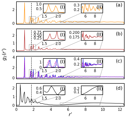
Figure 7: The pair correlation function g${}_{2}(r^{\prime})$ for (a) CMIPS (b) RC (c) NC and (d) LC. The black dashed line is drawn at $r^{\prime}=\sqrt{3}$. The system parameters for the four phases are the same as in Fig. 6. The magenta dashed curve in panel (c) corresponds to a NC system with lower $\nu=1.25$. Inset I zooms into $r^{\prime}\in(1.5,2.25)$. Inset II zooms into $r^{\prime}\in(5.25,9.5)$.

To characterize the structural ordering of the particles in different phases, the radial distribution function (RDF) $g_{2}$(r) is calculated. RDF is a measure of the probability of finding a particle at $r_{2}$ given a particle at $r_{1}$ with $r=|r_{2}$-$r_{1}|$. In two dimensions, 2$<n>g(r)d^{2}r$ gives the number of particles in $d^{2}r$, where $<n>$ is the mean number of particles in the unit area. RDF is plotted against the normalized radial distance $r^{\prime}=r/(2a_{0})$ in Fig. 7. Evidently, CMIPS, RC and NC show their largest peak at the nearest-neighbor(nn) distance $r^{\prime}=1$. The second and third peaks occur at $r^{\prime}=\sqrt{3}$ (second nn) and $r^{\prime}=2$ (third nn) respectively [see insets I of Fig. 7]. This indicates the presence of hexagonal close-packing (HCP). For LC, the major peaks occur before this distance as their constituents are more tightly packed than HCP.

Note that in NC, the minor peaks are less dense for higher $\nu$ (solid curve) compared to lower $\nu$ (dashed curve) [see inset I of Fig. 7 (c)]. This is an indication that the boundary is more rigid and particles experience more confinement for higher $\nu$ in the NC phase. Continuing to increase $\nu$ for a certain $\epsilon$ will lead to strict localization as in LC. This supports our observation of anomalous diffusivity in NC. Insets II of Fig. 7 zoom into the radial distances near the start of the next periodic valley. CMIPS shows long-range ordering, LC indicates periodicity in clustering but such information is inconclusive in RC and NC.

We characterize the orientational dynamics of particles by calculating the velocity auto-correlation function (VACF) of the particles defined by:

$$C_{v}(t)=<\cos(\phi(t_{0})-\phi(t+t_{0}))>-<\cos\phi(t+t_{0})>^{2}$$ (4)

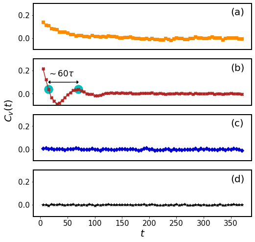
Figure 8: Variation of the particle velocity auto-correlation function C${}_{v}(t)$ for (a) CMIPS (b) RC (c) NC and (d) LC. This is calculated for $350\tau_{c}$ in the steady state. The system parameters for the four phases are the same as in Fig. 6

where the $<...>$ is the average over many reference times $t_{0}$, particles N and many independent realisations. VACF for the four phases is reported in Fig. 8. VACF exponentially decays for CMIPS [see Fig. 8 (a)]. Exponential fitting of the same yields the decay time: $t_{c}\sim 50\tau_{c}$. Hence, velocity has a long decay time for CMIPS phase, unlike MIPS vacf . The VACF shows clear oscillations for RC indicating rotational order in the system [see Fig. 8 (b)]. To support it, snapshots of a single cluster with a red tagged particle and its variation over time are shown in Fig. 4 (c). The time taken to complete one full cycle is annotated in Fig. 8 (b) by highlighting two velocities separated by $t_{4}-t_{1}=60\tau_{c}$. While it is the steepness of the valley ($\epsilon$) that drives the particles into periodic clusters, once the clusters are formed, the activity ensures the particle dynamics inside the cluster. However, moving tangentially along the radial layers of the cluster is the only means to minimize the surface potential. Thus, activity and steric forces alone contribute to the rotations in RC. Velocities of particles in NC and LC do not share a functional relationship, hence the VACF is almost zero [see Fig. 8 (c-d)].

CMIPS $\epsilon=$0.001		RC $\epsilon=$0.005		RC $\epsilon=$0.01
$\nu$	$\Omega(\nu,\epsilon)$	$\nu$	$\Omega(\nu,\epsilon)$	$\nu$	$\Omega(\nu,\epsilon)$
2.50	0.054	0.75	0.019	1.25	0.02
3.75	0.093	1.25	0.038	1.50	0.036
5.00	0.121	1.75	0.050	1.875	0.065
7.50	0.184	2.25	0.064	2.50	0.064
10.00	0.202	2.50	0.059	3.75	0.101

Table 1: The global angular velocity $\Omega(\nu,\epsilon)$ for some RC and CMIPS systems.

The handedness of any two nearest rotating clusters in RC are opposite [see Fig. 4 (a-b)]. The sense of rotation of a cluster is purely decided by the particles which are at the outer layer as they have the highest magnitude of instantaneous velocity in the cluster. The regions in which the exchange of particles is taking place between clusters are highlighted by red dashed circles in Fig. 4 (b). If a particle from a cluster is leaving to join one of the nearest clusters, it changes its sense of rotation to keep up with the new cluster. In this way, activity, steric repulsion, and periodic chemical concentration lead to synchronized rotations in the whole system.

The macroscopic clusters we obtained in CMIPS also rotate as a part or whole [refer Supplementary Material $S1$]. Hence our rotational states are from both CMIPS (macroscopic rotations) and RC (synchronized rotations). To characterize the extent of rotation we calculate the global angular velocity $\Omega(\nu,\epsilon)$:

$$\Omega(\nu,\epsilon)=<\frac{1}{N_{c}}\sum_{i=1}^{N_{c}}|\sum_{j=1}^{N_{c,j}}\frac{(\textbf{r}_{j}\times\textbf{v}_{j})|}{r_{j}^{2}}>$$ (5)

where $N_{c}$ denotes the number of valleys in the system (fixed for a certain $\lambda$); $N_{c,j}$ refers to the number of particles in the $i^{th}$ cluster computed by counting particles within a radial distance of $\lambda/8$ from the center of the $i^{th}$ valley. ${\bf r}_{j}$ is the position of the $j^{th}$ particle relative to the center of the valley and ${\bf v}_{j}$ is the instantaneous velocity of the $j^{th}$ particle. Table 1 reports the values of $\Omega$ for systems with such rotational order. $\Omega$ increases linearly with $\nu$ for both CMIPS and RC phases. Although both the phases have macroscopic rotations, the RC phase is additionally characterized by synchronized rotations.

IV Discussion

We have studied the dynamics and steady states of a collection of chemo-phoretically interacting ABPs for the case of a chemical potential that is quenched in time and periodic in space. The study elucidates the competition between activity and chemotaxis. In the extreme limits, when activity dominates we obtain chemotactic-MIPS i.e., CMIPS, and when chemotaxis dominates we obtain localized clusters having glassy dynamics. When the active force and the chemical force are comparable, particles arrange themselves into periodic clusters of finite length showing synchronized rotations about their centers.

We emphasize that in the case of synchronized rotations, a strict sense of handedness is picked up by a cluster without any intrinsic alignment interaction within the model. An interplay of time-reversal asymmetry and chemo-phoretic interactions between the repulsive disks is responsible for such collective rotations in the system. This phase may share some similarities with the dynamics of swarmalators in $1-$dimensional ring kevin1 ; kevin2 . We vouch for the reproducibility of our results for other kinds of time-quenched taxis, viz. phototaxis photo , viscotaxis visco , electrotaxis electro , thermotaxis thermo , etc. The observed rotations are more robust and are in contrast with swarms that generally have one cluster rotating about its center of mass swarm as a response to external obstacles or phoretic-motility vicseknatphys ; honeybee ; swarming .

While our study has focused on a purely symmetric quench, it will be interesting to study a system with spatially random or time-dependent chemotaxis. Such responses can alternatively be studied using the continuum theory of coarse-grained equations for slow variables tonertupre1998 ; catesprl2013 . Our results can also be tested in experiments by designing a patterned substrate for microswimmers. Such experiments can be crucial in understanding the chemotactic response of biological swimmers to the underlying medium.

V Author Contributions

The problem was designed by S.M. and numerically investigated by P.E. Both authors analyzed and interpreted the results. The manuscript was prepared by P.E. Both authors approved the final version of the manuscript.

VI Conflicts of interest

There are no conflicts of interest to declare.

VII Acknowledgements

P.E. acknowledges the support and the resources provided by PARAM Shivay Facility under the National Supercomputing Mission, Government of India at the Indian Institute of Technology, Varanasi. S.M. thanks DST-SERB India, MTR/2021/000438, and CRG/2021/006945 for financial support.

VIII Appendix

VIII.0.1 Non-interacting model: Variation in $\nu$

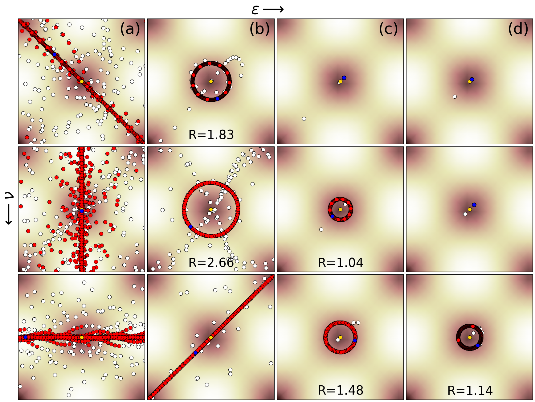
Figure 9: Single-particle model. Columns (a-d) show position of a single particle for all times in a simulation run for some system configurations: (a) $\epsilon=0.001$ (b) $\epsilon=0.005$ (c) $\epsilon=0.03$ (d) $\epsilon=0.05$ for $\nu=1.25,2.5$ and $5$. Colors and annotation have the same meaning as in Fig. 1.

References

- (1) J. Toner, Y. H. Tu, and S. Ramaswamy, Ann. Phys. (N.Y.), 318, 170 (2005).
- (2) T. Vicsek and A. Zafeiris, Phys. Rep. 517, 71 (2012).
- (3) M. C. Marchetti, J. F. Joanny, S. Ramaswamy, T. B. Liverpool, J. Prost, M. Rao, and R. S. Simha, Rev. Mod. Phys. 85, 1143 (2013).
- (4) C. Bechinger, R. D. Leonardo, H. Löwen, C. Reichhardt, G. Volpe, and G. Volpe, Rev. Mod. Phys. 88, 045006, 2016.
- (5) M. Poujade, E. Grasland-Mongrain, A. Hertzog, J. Jouanneau, P. Chavrier, B. Ladoux, A. Buguin, and P. Silberzan, PNAS 104, 15988–15993 (2007).
- (6) T. Feder, Physics today 60, 28 (2007).
- (7) D. Helbing, I. Farkas, and T. Vicsek, Nature 407, 487–490 (2000).
- (8) N. Bain and D. Bartolo, Science 363, 46–49 (2019).
- (9) D. S. Schloesser, D. Hollenbeck, and C. T. Kello, Sci Rep 11, 8492 (2021).
- (10) T. Vicsek, A. Czirók, E. Ben-Jacob, I. Cohen and O. Shochet, Phys. Rev. Lett., 75, 1226–1229 (1995).
- (11) H. Chaté, Annu. Rev. Condens. Mat., 11, 189–192 (2020).
- (12) B. Liebchenand and D. Levis, Phys. Rev. Lett., 119, 058002 (2017).
- (13) I. Theurkauff, C. Cottin-Bizonne, J. Palacci, C. Ybert, and L. Bocquet, Phys. Rev. Lett., 108, 268303 (2012).
- (14) S. Ro, Y. Kafri, M. Kardar, and J. Tailleur, Phys. Rev. Lett. 126, 048003 (2021).
- (15) O. Dauchot and H. Löwen, J. Chem. Phys. 151, 114901 (2019).
- (16) J. Toner, N. Guttenberg, and Y. Tu, Phys. Rev. E 98, 062604 (2018).
- (17) R. Das, M. Kumar, and S. Mishra, Phys. Rev. E 98, 060602(R) (2018).
- (18) V. Semwal, S. Dikshit, and S. Mishra, Eur. Phys. J. E 44, 20 (2021).
- (19) F. Peruani and I. S. Aranson, Phys. Rev. Lett. 120, 238101 (2018).
- (20) G. Volpe, I. Buttinoni, D. Vogt, Hans-Jürgen Kümmerer, and C. Bechinger, Soft Matter, 7, 8810 (2011).
- (21) W. Qi and M. Dijkstra, Soft Matter, 11, 2852 (2015).
- (22) B. Liebchen and H. Löwen, Acc. Chem. Res. 51, 2982 (2018).
- (23) H. Stark, Acc. Chem. Res. 51, 2681 (2018).
- (24) B. Liebchen, M. E. Cates, and D. Marenduzzo, Soft Matter, 12, 7259 (2016).
- (25) H. Zhao, A. Košmrlj and S. S. Datta, arXiv:2301.12345 (2023).
- (26) M. R. Nejada and A. Najafi, Soft Matter, 15, 3248 (2019).
- (27) F. Fadda, D. A. Matoz-Fernandez, R. van Roij, and S. Jabbari-Farouji, Soft Matter., 10, 1039 (2023).
- (28) J. Hu, A. Wysocki, R.G. Winkler, G. Gompper, Sci Rep 5, 9586 (2015).
- (29) M. Pelton, K. Ladavac, and D.G. Grier, Phys. Rev. E 70, 031108 (2004).
- (30) U. Choudhury, A.V. Straube, P. Fischer, J.G. Gibbs, and F. Hofling, New J. Phys. 19, 125010 (2017).
- (31) S. Pattanayak, R. Das, M. Kumar, and S. Mishra, Eur. Phys. J. E 42, 62 (2019).
- (32) P. Dolai, A. Simha, and S. Mishra, Soft Matter, 14, 6137 (2018).
- (33) Y. Fily and M. C. Marchetti, Phys. Rev. Lett. 108, 235702 (2012).
- (34) E. F. Keller and L. A. Segel, J. Theor. Biol., 26, 399 (1970).
- (35) E. F. Keller and L. A. Segel, J. Theor. Biol., 30, 225 (1971).
- (36) I. Buttinoni, J. Bialké, F. Kümmel, H. Löwen, C. Bechinger, and T. Speck, Phys. Rev. Lett. 110, 238301 (2013).
- (37) A. Baskaran and M. C. Marchetti, Phys. Rev. Lett. 101, 268101 (2008).
- (38) J. R. Howse, R. A. L. Jones, A. J. Ryan, T. Gough, R. Vafabakhsh, and R. Golestanian, Phys. Rev. Lett. 99, 048102 (2007).
- (39) M. Theers, E. Westphal, K. Qi, R. G. Winkler, and G Gompper, Soft Matter, 14, 8590 (2018).
- (40) K. P. O’Keeffe , H. Hong, and S. H. Strogatz, Nat Commun 8, 1504 (2017).
- (41) G. K. Sar, D. Ghosh, and K. O’Keeffe, Phys. Rev. E 107, 024215 (2023).
- (42) M. Mijalkov, A. McDaniel, J. Wehr, and Giovanni Volpe, Phys. Rev. X 6, 011008 (2016).
- (43) B. Liebchen, P. Monderkamp, B. ten Hagen, and H. Löwen, Phys. Rev. Lett. 120, 208002 (2018).
- (44) D. J. Cohen, W. J. Nelson, and M. M. Maharbiz, Nat. Mater. 13, 409 (2014).
- (45) R. Golestanian, Phys. Rev. Lett. 108, 038303 (2012).
- (46) T. Bäuerle, R. C. Löffler, and C. ’Bechinger, Nat Commun 11, 2547 (2020).
- (47) D. Vahabli and T. Vicsek, arXiv:2302.09439v1 (2023).
- (48) J. M. Peters, O. Peleg and, L. Mahadevan, J Exp Biol 225 (5):jeb242234 (2022).
- (49) M. Casiulis and D. Levine, Phys. Rev. E 106, 044611 (2022).
- (50) J. Toner and Y. Tu, Phys. Rev. E 58, 4828 (1998).
- (51) J. Stenhammar, A. Tiribocchi, R. J. Allen, D. Marenduzzo, and M. E. Cates, Phys. Rev. Lett. 111, 145702 (2013).
- (52) See Supplementary Materials for animations of CMIPS and RC phases.