3Mformer: Multi-order Multi-mode Transformer
for Skeletal Action Recognition

Abstract

Many skeletal action recognition models use GCNs to represent the human body by 3D body joints connected body parts. GCNs aggregate one- or few-hop graph neighbourhoods, and ignore the dependency between not linked body joints. We propose to form hypergraph to model hyper-edges between graph nodes (e.g., third- and fourth-order hyper-edges capture three and four nodes) which help capture higher-order motion patterns of groups of body joints. We split action sequences into temporal blocks, Higher-order Transformer (HoT) produces embeddings of each temporal block based on (i) the body joints, (ii) pairwise links of body joints and (iii) higher-order hyper-edges of skeleton body joints. We combine such HoT embeddings of hyper-edges of orders $1,...,r$ by a novel Multi-order Multi-mode Transformer (3Mformer) with two modules whose order can be exchanged to achieve coupled-mode attention on coupled-mode tokens based on ‘channel-temporal block’, ‘order-channel-body joint’, ‘channel-hyper-edge (any order)’ and ‘channel-only’ pairs. The first module, called Multi-order Pooling (MP), additionally learns weighted aggregation along the hyper-edge mode, whereas the second module, Temporal block Pooling (TP), aggregates along the temporal block mode. Our end-to-end trainable network yields state-of-the-art results compared to GCN-, transformer- and hypergraph-based counterparts.

1 Introduction

Action Recognition has applications in video surveillance, human-computer interaction, sports analysis, and virtual reality [52, 54, 53, 58, 24, 25, 55, 59, 40, 57, 56]. Different from video-based methods which mainly focus on modeling the spatio-temporal representations from RGB frames and/or optical flow [52, 54, 53, 58, 55, 25], skeleton sequences, representing a spatio-temporal evolution of 3D body joints, have been proven robust against sensor noises and effective in action recognition while being computationally and storage efficient [52, 53, 24, 59, 40, 57, 56]. The skeleton data is usually obtained by either localization of 2D/3D coordinates of human body joints with the depth sensors or pose estimation algorithms applied to videos [2]. Skeleton sequences enjoy (i) simple structural connectivity of skeletal graph and (ii) temporal continuity of 3D body joints evolving in time. While temporal evolution of each body joint is highly informative, embeddings of separate body joints are insensitive to relations between body parts. Moreover, while the links between adjacent 3D body joints (following the structural connectivity) are very informative as they model relations, these links represent highly correlated nodes in the sense of their temporal evolution. Thus, modeling larger groups of 3D body joints as hyper-edges can capture more complex spatio-temporal motion dynamics.

The existing graph-based models mainly differ by how they handle temporal information. Graph Neural Network (GNN) may encode spatial neighborhood of the node followed by aggregation by LSTM [46, 65]. Alternatively, Graph Convolutional Network (GCN) may perform spatio-temporal convolution in the neighborhood of each node [64]. Spatial GCNs perform convolution within one or two hop distance of each node, e.g., spatio-temporal GCN model called ST-GCN [64] models spatio-temporal vicinity of each 3D body joint. As ST-GCN applies convolution along structural connections (links between body joints), structurally distant joints, which may cover key patterns of actions, are largely ignored. ST-GCN captures ever larger neighborhoods as layers are added but suffers from oversmoothing that can be mitigated by linear GCNs [76, 78, 77].

Human actions are associated with interaction groups of skeletal joints, e.g., wrist alone, head-wrist, head-wrist-ankles, etc. The impact of these groups of joints on each action differs, and the degree of influence of each joint should be learned. Accordingly, designing a better model for skeleton data is vital given the topology of skeleton graph is suboptimal. While GCN can be applied to a fully-connected graph (i.e., 3D body joints as densely connected graph nodes), Higher-order Transformer (HoT) [21] has been proven more efficient.

Thus, we propose to use hypergraphs with hyper-edges of order $1$ to $r$ to effectively represent skeleton data for action recognition. Compared to GCNs, our encoder contains an MLP followed by three HoT branches that encode first-, second- and higher-order hyper-edges, i.e., set of body joints, edges between pairs of nodes, hyper-edges between triplets of nodes, etc. Each branch has its own learnable parameters, and processes temporal blocks one-by-one.

We notice that (i) the number of hyper-edges of $J$ joints grows rapidly with order $r$, i.e., $\binom{J}{i}$ for $i=1,...,r$, embeddings of the highest order dominate lower orders in terms of volume if such embeddings are merely concatenated, and (ii) long-range temporal dependencies of feature maps are insufficiently explored, as sequences are split into $\tau$ temporal blocks for computational tractability.

Merely concatenating outputs of HoT branches of orders $1$ to $r$, and across $\tau$ blocks, is sub-optimal. Thus, our Multi-order Multi-mode Transformer (3Mformer) with two modules whose order can be exchanged, realizes a variation of coupled-mode tokens based on ‘channel-temporal block’, ‘order-channel-body joint’, ‘channel-hyper-edge (any order)’ and ‘channel-only’ pairs. As HoT operates block-by-block, ‘channel-temporal block’ tokens and weighted hyper-edge aggregation in Multi-order Pooling (MP) help combine information flow block-wise. Various coupled-mode tokens help improve results further due to different focus of each attention mechanism. As the block-temporal mode needs to be aggregated (number of blocks varies across sequences), Temporal block Pooling (TP) can use rank pooling [13], second-order [33, 80, 60, 14, 68, 26, 41] or higher-order pooling [8, 25, 24, 70, 69].

In summary, our main contributions are listed as follows:

1. We model the skeleton data as hypergraph of orders $1$ to $r$ (set, graph and/or hypergraph), where human body joints serve as nodes. Higher-order Transformer embeddings of such formed hyper-edges represent various groups of 3D body joints and capture various higher-order dynamics important for action recognition.

2. As HoT embeddings represent individual hyper-edge order and block, we introduce a novel Multi-order Multi-mode Transformer (3Mformer) with two modules, Multi-order Pooling and Temporal block Pooling. Their goal is to form coupled-mode tokens such as ‘channel-temporal block’, ‘order-channel-body joint’, ‘channel-hyper-edge (any order)’ and ‘channel-only’, and perform weighted hyper-edge aggregation and temporal block aggregation.

Our 3Mformer outperforms other GCN- and hypergraph-based models on NTU-60, NTU-120, Kinetics-Skeleton and Northwestern-UCLA by a large margin.

Figure 1: Pipeline overview. Each sequence is split into $\tau$ temporal blocks $\mathbf{B}_{1},...,\mathbf{B}_{\tau}$. Subsequently, each block is embedded by a simple MLP into $\mathbf{X}_{1},...,\mathbf{X}_{\tau}$, which are passed to Higher-order Transformers (HoT ($n\!=\!1,...,r$)) in order to obtain feature tensors $\mathbf{\Phi}_{1},...,\mathbf{\Phi}_{\tau}$. These tensors are subsequently concatenated by $\odot$ along the hyper-edge mode into a multi-order feature tensor $\bm{\mathcal{M}}$. The final step is a Multi-order Multi-mode Transformer (3Mformer from Section 4), which contains two complementary branches, MP$\rightarrow$TP and TP$\rightarrow$MP, whose outputs are concatenated by $\odot$ and passed to the classifier. MP and TP perform the Coupled-mode Self-Attention (CmSA) with the so-called coupled-mode tokens, based on ‘channel-temporal block’, ‘order-channel-body joint’, ‘channel-hyper-edge’ and ‘channel-only’ pairs. To this end, MP contains also weighted pooling along hyper-edge mode by learnable matrix $\mathbf{H}$ (and $\mathbf{H}^{\prime}$ in another branch). TP contains also block-temporal pooling denoted by $g(\cdot)$ whose role is to capture block-temporal order with average, maximum, rank pooling, etc. In our experiments we show that such designed MP and TP are able to efficiently process hyper-edge feature representations from HoT branches. Appendix A shows full visualization of our 3Mformer.

2 Related Work

Below we describe popular action recognition models for skeletal data.

Graph-based models. Popular GCN-based models include the Attention enhanced Graph Convolutional LSTM network (AGC-LSTM) [46], the Actional-Structural GCN (AS-GCN) [30], Dynamic Directed GCN (DDGCN) [27], Decoupling GCN with DropGraph module [5], Shift-GCN [6], Semantics-Guided Neural Networks (SGN) [67], AdaSGN [45], Context Aware GCN (CA-GCN) [71], Channel-wise Topology Refinement Graph Convolution Network (CTR-GCN) [4] and a family of Efficient GCN (EfficientGCN-Bx) [47]. Although GCN-based models enjoy good performance, they have shortcomings, e.g., convolution and/or pooling are applied over one- or few-hop neighborhoods, e.g., ST-GCN [64], according to the human skeleton graph (body joints linked up according to connectivity of human body parts). Thus, indirect links between various 3D body joints such as hands and legs are ignored. In contrast, our model is not restricted by the structure of typical human body skeletal graph. Instead, 3D body joints are nodes which form hyper-edges of orders $1$ to $r$.

Hypergraph-based models. Pioneering work on capturing groups of nodes across time uses tensors [24] to represent the 3D human body joints to exploit the kinematic relations among the adjacent and non-adjacent joints. Representing the human body as a hypergraph is adopted in [35] via a semi-dynamic hypergraph neural network that captures richer information than GCN. A hypergraph GNN [15] captures both spatio-temporal information and higher-order dependencies for skeleton-based action recognition. Our work is somewhat closely related to these works, but we jointly use hypergraphs of order $1$ to $r$ to obtain rich hyper-edge embeddings based on Higher-order Transformers.

Transformer-based models. Action recognition with transformers includes self-supervised video transformer [42] that matches the features from different views (a popular strategy in self-supervised GCNs [74, 75]), the end-to-end trainable Video-Audio-Text-Transformer (VATT) [1] for learning multi-model representations from unlabeled raw video, audio and text through the multimodal contrastive losses, and the Temporal Transformer Network with Self-supervision (TTSN) [72]. Motion-Transformer [7] captures the temporal dependencies via a self-supervised pre-training on human actions, Masked Feature Prediction (MaskedFeat) [61] pre-trained on unlabeled videos with MViT-L learns abundant visual representations, and video-masked autoencoder (VideoMAE) [48] with vanilla ViT uses the masking strategy. In contrast to these works, we use three HoT branches of model [21], and we model hyper-edges of orders $1$ to $r$ by forming several multi-mode token variations in 3Mformer.

Attention. In order to improve feature representations, attention captures relationship between tokens. Natural language processing and computer vision have driven recent developments in attention mechanisms based on transformers [49, 11]. Examples include the hierarchical Cross Attention Transformer (CAT) [32], Cross-attention by Temporal Shift with CNNs [16], Cross-Attention Multi-Scale Vision Transformer (CrossViT) for image classification [3] and Multi-Modality Cross Attention (MMCA) Network for image and sentence matching [63]. In GNNs, attention can be defined over edges [50, 66] or over nodes [29]. In this work, we use the attention with hyper-edges of several orders from HoT branches serving as tokens, and coupled-mode attention with coupled-mode tokens based on ‘channel-temporal block’, ‘order-channel-body joint’, ‘channel-hyper-edge (any order)’ and ‘channel-only’ pairs formed in 3Mformer.

3 Background

Below we describe foundations necessary for our work.

Notations. $\mathcal{I}_{K}$ stands for the index set $\{1,2,...,K\}$. Regular fonts are scalars; vectors are denoted by lowercase boldface letters, e.g., x; matrices by the uppercase boldface, e.g., M; and tensors by calligraphic letters, e.g., $\bm{\mathcal{M}}$. An $r$th-order tensor is denoted as $\bm{\mathcal{M}}\in\mathbb{R}^{I_{1}\times I_{2}\times...\times I_{r}}$, and the mode-$m$ matricization of $\bm{\mathcal{M}}$ is denoted as $\bm{\mathcal{M}}_{(m)}\in\mathbb{R}^{I_{m}\times(I_{1}...I_{m-1}I_{m+1}...I_{r})}$.

Transformer layers [49, 11]. A transformer encoder layer $f\!:\mathbb{R}^{J\times d}\rightarrow\mathbb{R}^{J\times d}$ consists of two sub-layers: (i) a self-attention $a\!:\mathbb{R}^{J\times d}\rightarrow\mathbb{R}^{J\times d}$ and (ii) an element-wise feed-forward $\text{MLP}\!:\mathbb{R}^{J\times d}\rightarrow\mathbb{R}^{J\times d}$. For a set of $J$ nodes with ${\bf X}\!\in\!\mathbb{R}^{J\times d}$, where ${\bf x}_{i}$ is a feature vector of node $i$, a transformer layer computes:

$$a({\bf x}_{i})\!=\!{\bf x}_{i}\!+\!\sum_{h=1}^{H}\sum_{j=1}^{J}\alpha_{ij}^{h}{\bf x}_{j}{\bf W}_{h}^{V}{\bf W}_{h}^{O},$$ (1)

$$f({\bf x}_{i})\!=\!a({\bf x}_{i})\!+\!\text{MLP}(a({\bf X}))_{i},$$ (2)

where $H$ and $d_{H}$ denote respectively the number of heads and the head size, ${\bm{\alpha}}^{h}\!=\!\sigma\big{(}{\bf X}{\bf W}_{h}^{Q}({\bf X}{\bf W}_{h}^{K})^{\top}\big{)}$ is the attention coefficient, ${\bf W}_{h}^{O}\!\in\!\mathbb{R}^{d_{H}\times d}$, and ${\bf W}_{h}^{V}$, ${\bf W}_{h}^{K}$, ${\bf W}_{h}^{Q}\!\in\!\mathbb{R}^{d\times d_{H}}$.

Higher-order transformer layers [21]. Let the HoT layer be $f_{m\rightarrow n}\!:\mathbb{R}^{J^{m}\times d}\!\rightarrow\!\mathbb{R}^{J^{n}\times d}$ with two sub-layers: (i) a higher-order self-attention $a_{m\rightarrow n}\!:\mathbb{R}^{J^{m}\times d}\!\rightarrow\!\mathbb{R}^{J^{n}\times d}$ and (ii) a feed-forward $\text{MLP}_{n\rightarrow n}\!:\mathbb{R}^{J^{n}\times d}\!\rightarrow\!\mathbb{R}^{J^{n}\times d}$. Moreover, let indexing vectors ${\bf i}\in\mathcal{I}_{J}^{m}\equiv\mathcal{I}_{J}\!\times\!\mathcal{I}_{J}\!\times\!...\!\times\!\mathcal{I}_{J}$ ($m$ modes) and ${\bf j}\in\mathcal{I}_{J}^{n}\equiv\mathcal{I}_{J}\!\times\!\mathcal{I}_{J}\!\times\!...\!\times\!\mathcal{I}_{J}$ ($n$ modes). For the input tensor ${\bf X}\!\in\!\mathbb{R}^{J^{m}\times d}$ with hyper-edges of order $m$, a HoT layer evaluates:

$$a_{m\rightarrow n}({\bf X})_{\bm{j}}\!=\!\sum_{h=1}^{H}\sum_{\mu}\sum_{\bm{i}}{\bm{\alpha}}_{{\bm{i}},{\bm{j}}}^{h,\mu}{\bf X}_{\bm{i}}{\bf W}_{h,\mu}^{V}{\bf W}_{h,\mu}^{O}$$ (3)

$$\text{MLP}_{n\rightarrow n}(a_{m\rightarrow n}({\bf X}))\!=\!\text{L}_{n\rightarrow n}^{2}(\text{ReLU}(\text{L}_{n\rightarrow n}^{1}(a_{m\rightarrow n}({\bf X})))),$$ (4)

$$f_{m\rightarrow n}({\bf X})\!=\!a_{m\rightarrow n}({\bf X})\!+\!\text{MLP}_{n\!\rightarrow\!n}(a_{m\rightarrow n}({\bf X})),$$ (5)

where ${\bm{\alpha}}^{h,\mu}\!\in\!\mathbb{R}^{J^{m+n}}$ is the so-called attention coefficient tensor with multiple heads, and ${\bm{\alpha}}^{h,\mu}_{{\bf i},{\bf j}}\!\in\!\mathbb{R}^{J}$ is a vector, ${\bf W}_{h,\mu}^{V}\!\in\!\mathbb{R}^{d\times d_{H}}$ and ${\bf W}_{h,\mu}^{O}\!\in\!\mathbb{R}^{d_{H}\times d}$ are learnable parameters. Moreover, $\mu$ indexes over the so-called equivalence classes of order-$(m\!+\!n)$ in the same partition of nodes, $\text{L}_{n\rightarrow n}^{1}\!:\mathbb{R}^{J^{n}\times d}\rightarrow\mathbb{R}^{J^{n}\times d_{F}}$ and $\text{L}_{n\rightarrow n}^{2}\!:\mathbb{R}^{J^{n}\times d_{F}}\rightarrow\mathbb{R}^{J^{n}\times d}$ are equivariant linear layers and $d_{F}$ is the hidden dimension.

To compute each attention tensor ${\bm{\alpha}}^{h,\mu}\!\in\!\mathbb{R}^{J^{m+n}}$ from the input tensor ${\bf X}\!\in\!\mathbb{R}^{J^{m}\times d}$ of hyper-edges of order $m$, from the higher-order query and key, we obtain:

$${{\bm{\alpha}}_{{\bm{i}},{\bm{j}}}^{h,\mu}}\!=\!\begin{cases}\frac{\sigma({\bf Q}_{\bm{j}}^{h,\mu},{\bf K}_{\bm{i}}^{h,\mu})}{Z_{\bm{j}}}\;\quad({\bm{i}},{\bm{j}})\!\in\!\mu\\ \quad\quad 0\quad\quad\;\text{otherwise},\end{cases}$$ (6)

where ${\bf Q}^{\mu}\!=\!\text{L}_{m\rightarrow n}^{\mu}({\bf X})$, ${\bf K}^{\mu}\!=\!\text{L}_{m\rightarrow m}^{\mu}({\bf X})$, and normalization constant $Z_{\bm{j}}\!=\!\sum_{{\bm{i}}:({\bm{i}},{\bm{j}})\in\mu}\sigma({\bf Q}_{\bm{j}}^{\mu},{\bf K}_{\bm{i}}^{\mu})$. Finally, kernel attention in Eq. (6) can be approximated with RKHS feature maps $\psi\in\mathbb{R}_{+}^{d_{K}}$ for efficacy as $d_{K}\ll d_{H}$. Specifically, we have $\sigma\big{(}{\bf Q}_{\bm{j}}^{h,\mu},{\bf K}_{\bm{i}}^{h,\mu}\big{)}\approx{\bm{\psi}}\big{(}{\bf Q}_{\bm{j}}^{h,\mu}\big{)}^{\top}{\bm{\psi}}\big{(}{\bf K}_{\bm{i}}^{h,\mu}\big{)}$ as in [19, 10]. We choose the performer kernel [10] due to its good performance.

As query and key tensors are computed from the input tensor ${\bf X}$ using the equivariant linear layers, the transformer encoder layer $f_{m\rightarrow n}$ satisfies the permutation equivariance.

4 Approach

Skeletal Graph [64] and Skeletal Hypergraph [35, 15] are popular for modeling edges and hyper-edges. In this work, we use the Higher-order Transformer (HoT) [21] as a backbone encoder.

4.1 Model Overview

Fig. 1 shows that our framework contains a simple 3-layer MLP unit (FC, ReLU, FC, ReLU, Dropout, FC), three HoT blocks with each HoT for each type of input (i.e., body joint feature set, graph and hypergraph of body joints), followed by Multi-order Multi-mode Transformer (3Mformer) with two modules (i) Multi-order Pooling (MP) and (ii) Temporal block Pooling (TP). The goal of 3Mformer is to form coupled-mode tokens (explained later) such as ‘channel-temporal block’, ‘order-channel-body joint’, ‘channel-hyper-edge (any order)’ and ‘channel-only’, and perform weighted hyper-edge aggregation and temporal block aggregation. Their outputs are further concatenated and passed to an FC layer for classification.

MLP unit. The MLP unit takes $T$ neighboring frames, each with $J$ 2D/3D skeleton body joints, forming one temporal block. In total, depending on stride $S$, we obtain some $\tau$ temporal blocks (a block captures the short-term temporal evolution), In contrast, the long-term temporal evolution is modeled with HoT and 3Mformer. Each temporal block is encoded by the MLP into a $d\!\times\!J$ dimensional feature map.

HoT branches. We stack $r$ branches of HoT, each taking embeddings ${\bf X}_{t}\in\mathbb{R}^{d\!\times\!J}$ where $t\in\mathcal{I}_{\tau}$ denotes a temporal block. HoT branches output hyper-edge feature representations of size $m\in\mathcal{I}_{r}$ as ${\bf\Phi}^{\prime}_{m}\in\mathbb{R}^{J^{m}\times d^{\prime}}$ for order $m\in\mathcal{I}_{r}$.

For the first-, second- and higher-order stream outputs ${\bf\Phi}^{\prime}_{1},...,{\bf\Phi}^{\prime}_{r}$, we (i) swap feature channel and hyper-edge modes, (ii) extract the upper triangular of tensors, and we concatenate along the block-temporal mode, so we have ${\bf\Phi}_{m}\in\mathbb{R}^{d^{\prime}\times N_{E_{m}}\times\tau}$, where $N_{E_{m}}\!=\!\binom{J}{m}$. Subsequently, we concatenate ${\bf\Phi}_{1},...,{\bf\Phi}_{r}$ along the hyper-edge mode and obtain a multi-order feature tensor ${\color[rgb]{0,0,0}\bm{\mathcal{M}}}\!\in\!\mathbb{R}^{d^{\prime}\!\times\!N\!\times\!\tau}$ where the total number of hyper-edges across all orders is $N=\sum_{m=1}^{r}\binom{J}{m}$.

3Mformer. Our Multi-order Multi-mode Transformer (3Mformer) with Coupled-mode Self-Attention (CmSA) is used for the fusion of information flow inside the multi-order feature tensor ${\bm{\mathcal{M}}}$, and finally, the output from 3Mformer is passed to a classifier for classification.

4.2 Coupled-mode Self-Attention

Coupled-mode tokens. We are inspired by the attentive regions of the one-class token in the standard Vision Transformer (ViT) [49] that can be leveraged to form a class-agnostic localization map. We investigate if the transformer model can also effectively capture the coupled-mode attention for more discriminative classification tasks, e.g., tensorial skeleton-based action recognition by learning the coupled-mode tokens within the transformer. To this end, we propose a Multi-order Multi-mode Transformer (3Mformer), which uses coupled-mode tokens to jointly learn various higher-order motion dynamics among channel-, block-temporal-, body joint- and order-mode. Our 3Mformer can successfully produce coupled-mode relationships from CmSA mechanism corresponding to different tokens. Below we introduce our CmSA.

Given the order-$r$ tensor $\bm{\mathcal{M}}\in\mathbb{R}^{I_{1}\times I_{2}\times...\times I_{r}}$, to form the joint mode token, we perform the mode-$m$ matricization of $\bm{\mathcal{M}}$ to obtain $\textbf{M}\equiv\bm{\mathcal{M}}_{(m)}^{\top}\in\mathbb{R}^{(I_{1}...I_{m-1}I_{m+1}...I_{r})\times I_{m}}$, and the coupled-token for M is formed. For example, for a given 3rd-order tensor that has feature channel-, hyper-edge- and temporal block-mode, we can form ‘channel-temporal block’, ‘channel-hyper-edge (any order)’ and ‘channel-only’ pairs; and if the given tensor is used as input and outputs a new tensor which produces new mode, e.g., body joint-mode, we can form the ‘order-channel-body joint’ token. In the following sections, for simplicity, we use reshape for the matricization of tensor to form different types of coupled-mode tokens. Our CmSA is given as:

$$\!\!a({\bf Q},{\bf K},{\bf V})\!=\!\text{SoftMax}\left(\frac{{\bf Q}{\bf K}^{\top}}{\sqrt{d_{K}}}\right)\!{\bf V},\!$$ (7)

where $\sqrt{d_{K}}$ is the scaling factor, ${\bf Q}\!=\!{\bf W}^{q}{\bf M}$, ${\bf K}\!=\!{\bf W}^{k}{\bf M}$ and ${\bf V}\!=\!{\bf W}^{v}{\bf M}$ are the query, key and value, respectively, and $\textbf{M}\equiv\bm{\mathcal{M}}_{(m)}^{\top}$. Moreover, ${\bf Q}$, ${\bf K}$, ${\bf V}\!\in\!\mathbb{R}^{(I_{1}...I_{m-1}I_{m+1}...I_{r})\times I_{m}}$ and ${\bf W}^{q}$, ${\bf W}^{k}$, ${\bf W}^{v}\!\in\!\mathbb{R}^{(I_{1}...I_{m-1}I_{m+1}...I_{r})\times(I_{1}...I_{m-1}I_{m+1}...I_{r})}$ are learnable weights. We notice that various coupled-mode tokens have different ‘focus’ of attention mechanisms, and we apply them in our 3Mformer for the fusion of multi-order feature representations.

4.3 Multi-order Multi-mode Transformer

Below we introduce Multi-order Multi-mode Transformer (3Mformer) with Multi-order Pooling (MP) block and Temporal block Pooling (TP) block, which are cascaded into two branches (i) MP$\rightarrow$TP and (ii) TP$\rightarrow$MP, to achieve different types of coupled-mode tokens.

4.3.1 Multi-order Pooling (MP) Module

CmSA in MP. We reshape the multi-order feature representation ${\color[rgb]{0,0,0}\bm{\mathcal{M}}}\!\in\!\mathbb{R}^{d^{\prime}\!\times\!N\!\times\!\tau}$ into ${\bf M}\!\in\!\mathbb{R}^{d^{\prime}\tau\!\times\!N}$ (or reshape the output from TP explained later into ${\bf M}^{\prime}\!\in\!\mathbb{R}^{d^{\prime}\!\times\!N}$) to let the model attend to different types of feature representations. Let us simply denote $d^{\prime\prime}\!=\!d^{\prime}\tau$ (or $d^{\prime\prime}\!=\!d^{\prime}$) depending on the source of input. We form an coupled-mode self-attention (if $d^{\prime\prime}=d^{\prime}\tau$, we have, i.e., ‘channel-temporal block’ token; if $d^{\prime\prime}=d^{\prime}$, we have ‘channel-only’ token):

$$\!\!a_{\text{MP}}({\bf Q}_{\text{MP}},{\bf K}_{\text{MP}},{\bf V}_{\text{MP}})\!=\!\text{SoftMax}\left(\frac{{\bf Q}_{\text{MP}}{\bf K}_{\text{MP}}^{\top}}{\sqrt{d_{K_{\text{MP}}}}}\right)\!{\bf V}_{\text{MP}},\!$$ (8)

where $\sqrt{d_{K_{\text{MP}}}}$ is the scaling factor, ${\bf Q}_{\text{MP}}\!=\!{\bf W}_{\text{MP}}^{q}{\bf M}$, ${\bf K}_{\text{MP}}\!=\!{\bf W}_{\text{MP}}^{k}{\bf M}$ and ${\bf V}_{\text{MP}}\!=\!{\bf W}_{\text{MP}}^{v}{\bf M}$ (we can use here ${\bf M}$ or ${\bf M}^{\prime}$) are the query, key and value. Moreover, ${\bf Q}_{\text{MP}}$, ${\bf K}_{\text{MP}}$, ${\bf V}_{\text{MP}}\!\in\!\mathbb{R}^{d^{\prime\prime}\times N}$ and ${\bf W}_{\text{MP}}^{q}$, ${\bf W}_{\text{MP}}^{k}$, ${\bf W}_{\text{MP}}^{v}\!\in\!\mathbb{R}^{d^{\prime\prime}\times d^{\prime\prime}}$ are learnable weights. Eq. (8) is a self-attention layer which reweighs ${\bf V}_{\text{MP}}$ based on the correlation between ${\bf Q}_{\text{MP}}$ and ${\bf K}_{\text{MP}}$ token embeddings of so-called coupled-mode tokens.

Weighted pooling. Attention layer in Eq. (8) produces feature representation ${\bf O}_{\text{MP}}\!\in\!\mathbb{R}^{d^{\prime\prime}\times N}$ to enhance the relationship between for example feature channels and body joints. Subsequently, we handle the impact of hyper-edges of multiple orders by weighted pooling along hyper-edges of order $m\in\mathcal{I}_{r}$:

$${\bf O}_{\text{MP}}^{*(m)}\!=\!{\bf O}_{\text{MP}}^{(m)}{\bf H}^{(m)}\!\in\!\mathbb{R}^{d^{\prime\prime}\times J},$$ (9)

where ${\bf O}_{\text{MP}}^{(m)}\!\in\!\mathbb{R}^{d^{\prime\prime}\times N_{E_{m}}}$ is simply extracted from ${\bf O}_{\text{MP}}$ for hyper-edges of order $m$, and matrices ${\bf H}^{(m)}\!\in\!\mathbb{R}^{N_{E_{m}}\times J}$ are learnable weights to perform weighted pooling along hyper-edges of order $m$. Finally, we obtain ${\bf O}_{\text{MP}}^{*}\!\in\!\mathbb{R}^{r{d^{\prime\prime}\times J}}$ by simply concatenating ${\bf O}_{\text{MP}}^{*(1)},...,{\bf O}_{\text{MP}}^{*(r)}$. If we used the input to MP from TP, then we denote the output of MP as ${{\bf O}^{\prime}}_{\text{MP}}^{*}$.

4.3.2 Temporal block Pooling (TP) Module

CmSA in TP. Firstly, we reshape the multi-order feature representation ${\color[rgb]{0,0,0}\bm{\mathcal{M}}}\!\in\!\mathbb{R}^{d^{\prime}\!\times\!N\!\times\!\tau}$ into ${\bf M}\!\in\!\mathbb{R}^{d^{\prime}N\!\times\!\tau}$ (or reshape the output from MP into ${\bf M}^{\prime\prime}\!\in\!\mathbb{R}^{rd^{\prime}J\!\times\!\tau}$). For simplicity, we denote $d^{\prime\prime\prime}\!=\!d^{\prime}N$ in the first case and $d^{\prime\prime\prime}\!=\!rd^{\prime}J$ in the second case. As the first mode of reshaped input serves to form tokens, they are again coupled-mode tokens, e.g., ‘channel-hyper-edge’ and ‘order-channel-body joint’ tokens, respectively. Moreover, TP also performs pooling along block-temporal mode (along $\tau$). We form an coupled-mode self-attention:

$$a_{\text{TP}}({\bf Q}_{\text{TP}},{\bf K}_{\text{TP}},{\bf V}_{\text{TP}})\!=\!\text{SoftMax}\left(\frac{{\bf Q}_{\text{TP}}{\bf K}_{\text{TP}}^{\top}}{\sqrt{d_{K_{\text{TP}}}}}\right)\!{\bf V}_{\text{TP}},$$ (10)

where $\sqrt{d_{K_{\text{TP}}}}$ is the scaling factor, ${\bf Q}_{\text{TP}}\!=\!{\bf W}_{\text{TP}}^{q}{\bf M}$, ${\bf K}_{\text{TP}}\!=\!{\bf W}_{\text{TP}}^{k}{\bf M}$ and ${\bf V}_{\text{TP}}\!=\!{\bf W}_{\text{TP}}^{v}{\bf M}$ (we can use here ${\bf M}$ or ${\bf M}^{\prime\prime}$) are the query, key and value. Moreover, ${\bf Q}_{\text{TP}}$, ${\bf K}_{\text{TP}}$, ${\bf V}_{\text{TP}}\!\in\!\mathbb{R}^{d^{\prime\prime\prime}\times\tau}$ and ${\bf W}_{\text{TP}}^{q}$, ${\bf W}_{\text{TP}}^{k}$, ${\bf W}_{\text{TP}}^{v}\!\in\!\mathbb{R}^{d^{\prime\prime\prime}\times d^{\prime\prime\prime}}$ are learnable weights. Eq. (10) reweighs ${\bf V}_{\text{TP}}$ based on the correlation between ${\bf Q}_{\text{TP}}$ and ${\bf K}_{\text{TP}}$ token embeddings of coupled-mode tokens (‘channel-hyper-edge’ or ‘order-channel-body joint’). The output of attention is the temporal representation ${\bf O}_{\text{TP}}\!\in\!\mathbb{R}^{d^{\prime\prime\prime}\times\tau}$. If we used ${\bf M}^{\prime\prime}$ as input, we denote the output as ${\bf O}^{\prime\prime}_{\text{TP}}$.

Pooling step. Given the temporal representation ${\bf O}_{\text{TP}}\!\in\!\mathbb{R}^{d^{\prime\prime\prime}\!\times\!\tau}$ (or ${\bf O}^{\prime\prime}_{\text{TP}}$), we apply pooling along the block-temporal mode to obtain compact feature representations independent of length (block count $\tau$) of skeleton sequence. There exist many pooling operations including first-order, e.g., average, maximum, sum pooling, second-order [80, 60] such as attentional pooling [14], higher-order (tri-linear) [8, 25] and rank pooling [13]. The output after pooling is ${\bf O}^{*}_{\text{TP}}\!\in\!\mathbb{R}^{d^{\prime\prime\prime}}\!$ (or ${{\bf O}^{\prime\prime}}^{*}_{\text{TP}}$).

4.3.3 Model Variants

We devise four model variants by different stacking of MP with TP, with the goal of exploiting attention with different kinds of coupled-mode tokens:

1. Single-branch: MP followed by TP, denoted MP$\rightarrow$TP, (Fig. 1 top right branch).

2. Single-branch: TP followed by MP, denoted TP$\rightarrow$MP, (Fig. 1 bottom right branch).

3. Two-branch (our 3Mformer, Fig. 1) which concatenates outputs of MP$\rightarrow$TP and TP$\rightarrow$MP.

4. We also investigate only MP or TP module followed by average pooling or an FC layer.

The outputs from MP$\rightarrow$TP and TP$\rightarrow$MP have exactly the same feature dimension ($\mathbb{R}^{rd^{\prime}J}$, after reshaping into vector). For two-branch (our 3Mformer), we simply concatenate these outputs ($\mathbb{R}^{2rd^{\prime}J}$, after concatenation). These vectors are forwarded to the FC layer to learn a classifier.

5 Experiments

5.1 Datasets and Protocols

(i) NTU RGB+D (NTU-60) [43] contains 56,880 video sequences.This dataset has variable sequence lengths and high intra-class variations. Each skeleton sequence has 25 joints and there are no more than two human subjects in each video. Two evaluation protocols are: (i) cross-subject (X-Sub) and (ii) cross-view (X-View).

(ii) NTU RGB+D 120 (NTU-120) [34], an extension of NTU-60, contains 120 action classes (daily/health-related), and 114,480 RGB+D video samples captured with 106 distinct human subjects from 155 different camera viewpoints. There are also two evaluation protocols: (i) cross-subject (X-Sub) and (ii) cross-setup (X-Set).

(iii) Kinetics-Skeleton, based on Kinetics [20], is large-scale dataset with 300,000 video clips and up to 400 human actions collected from YouTube. This dataset involves human daily activities, sports scenes and complex human-computer interaction scenes. Since Kinetics only provides raw videos without the skeletons, ST-GCN [64] uses the publicly available OpenPose toolbox [2] to estimate and extract the location of 18 human body joints on every frame in the clips. We use their released skeleton data to evaluate our model. Following the standard evaluation protocol, we report the Top-1 and Top-5 accuracies on the validation set.

(iv) Northwestern-UCLA [51] was captured by 3 Kinect cameras simultaneously from multiple viewpoints. It contains 1494 video clips covering 10 actions. Each action is performed by 10 different subjects. We follow the same evaluation protocol as [51]: training split is formed from the first two cameras, and testing split from the last camera.

5.2 Experimental Setup

We use PyTorch and 1$\times$Titan RTX 3090 for experiments. We use the Stochastic Gradient Descent (SGD) with momentum 0.9, cross-entropy as the loss, weight decay of 0.0001 and batch size of 32. The learning rate is set to 0.1 initially. On NTU-60 and NTU-120, the learning rate is divided by 10 at the 40th and 50th epoch, and the training process ends at the 60th epoch. On Kinetics-Skeleton, the learning rate is divided by 10 at the 50th and 60th epoch, and the training finishes at the 80th epoch. We took 20% of training set for validation to tune hyperparameters. All models have fixed hyperparameters with 2 and 4 layers for NTU-60/NTU-120 and Kinetics-Skeleton, respectively. The hidden dimensions is set to 16 for all 3 datasets. We use 4 attention heads for NTU-60 and NTU-120, and 8 attention heads for Kinetics-Skeleton. To form each video temporal block, we simply choose temporal block size to be 10 and stride to be 5 to allow a 50% overlap between consecutive temporal blocks. For Northwestern-UCLA, the batch size is 16. We adopted the data pre-processing in [6].

5.3 Ablation Study

Search for the single best order $n$. Table 1 shows our analysis regarding the best order $n$. In general, increasing the order $n$ improves the performance (within $\sim$ 0.5% on average), but causing higher computational cost, e.g., the number of hyper-edges for the skeletal hypergraph of order $n\!=\!4$ is 3060 on Kinetics-Skeleton. We also notice that combining orders 3 and 4 yields very limited improvements. The main reasons are: (i) reasonable order $n$, e.g., $n=3$ or 4 improves accuracy as higher-order motion patterns are captured which are useful for classification-related tasks (ii) further increasing order $n$, e.g., $n=5$ introduces patterns in feature representations that rarely repeat even for the same action class. Considering the cost and performance, we choose the maximum order $r\!=\!3$ ($n=1,2,3$) in the following experiments unless specified otherwise.

Table 1: Search for the single best order $n$ of hypergraph (except for $n\!=\!3\,\&\,4$ where we check if $n\!=\!3\,\&\,4$ are complementary).

Order-$n$	NTU-60		NTU-120		Kinetics-Skel.
	X-Sub	X-View	X-Sub	X-Set	Top-1 acc.
$n=1$	78.5	86.3	75.3	77.9	32.0
$n=2$	83.0	89.2	86.2	88.3	37.1
$n=3$	91.3	97.0	87.5	89.7	39.5
$n=4$	91.5	97.1	87.8	90.0	40.1
$n=5$	91.4	97.3	87.8	90.0	40.3
$n=3~{}\&~{}4$	91.6	97.2	87.6	90.3	40.5

Table 2: Evaluations of our model variants with/without MP and/or TP. Baseline in the table denotes the backbone (MLP unit + HoTs) without the use of either MP or TP module.

Variants	NTU-60		NTU-120		Kinetics-Skel.
	X-Sub	X-View	X-Sub	X-Set	Top-1 acc.
Baseline	89.8	91.4	86.5	87.0	38.6
+ TP only	91.2	93.8	87.5	88.6	39.8
+ MP only	92.0	94.3	88.7	89.7	40.3
+ MP$\rightarrow$TP	93.0	96.1	90.8	91.7	45.7
+ TP$\rightarrow$MP	92.6	95.8	90.2	91.1	44.0
+ 2-branch(3Mformer)	94.8	98.7	92.0	93.8	48.3

Table 3: Experimental results on NTU-60, NTU-120 and Kinetics-Skeleton.

	Method	Venue	NTU-60			NTU-120			Kinetics-Skeleton
			X-Sub	X-View		X-Sub	X-Set		Top-1	Top-5
Graph-based	TCN [22]	CVPRW’17	-	-		-	-		20.3	40.0
	ST-GCN [64]	AAAI’18	81.5	88.3		70.7	73.2		30.7	52.8
	AS-GCN [30]	CVPR’19	86.8	94.2		78.3	79.8		34.8	56.5
	2S-AGCN [44]	CVPR’19	88.5	95.1		82.5	84.2		36.1	58.7
	NAS-GCN [37]	AAAI’20	89.4	95.7		-	-		37.1	60.1
	Sym-GNN [31]	TPAMI’22	90.1	96.4		-	-		37.2	58.1
	Shift-GCN [6]	CVPR’20	90.7	96.5		85.9	87.6		-	-
	MS-G3D [36]	CVPR’20	91.5	96.2		86.9	88.4		38.0	60.9
	CTR-GCN [4]	ICCV’21	92.4	96.8		88.9	90.6		-	-
	InfoGCN [9]	CVPR’22	93.0	97.1		89.8	91.2		-	-
	PoseConv3D [12]	CVPR’22	94.1	97.1		86.9	90.3		47.7	-
Hypergraph-based	Hyper-GNN [15]	TIP’21	89.5	95.7		-	-		37.1	60.0
	DHGCN [62]	CoRR’21	90.7	96.0		86.0	87.9		37.7	60.6
	Selective-HCN [79]	ICMR’22	90.8	96.6		-	-		38.0	61.1
	SD-HGCN [17]	ICONIP’21	90.9	96.7		87.0	88.2		37.4	60.5
Transformer-based	ST-TR [39]	CVIU’21	90.3	96.3		85.1	87.1		38.0	60.5
	MTT [23]	LSP’21	90.8	96.7		86.1	87.6		37.9	61.3
	4s-GSTN [18]	Symmetry’22	91.3	96.6		86.4	88.7		-	-
	STST [73]	ACM MM’21	91.9	96.8		-	-		38.3	61.2
2-11	3Mformer (with avg-pool, ours)		92.0	97.3		88.0	90.1		43.1	65.2
	3Mformer (with max-pool, ours)		92.1	97.8		-	-		-	-
	3Mformer (with attn-pool, ours)		94.2	98.5		89.7	92.4		45.7	67.6
	3Mformer (with tri-pool, ours)		94.0	98.5		91.2	92.7		47.7	71.9
	3Mformer (with rank-pool, ours)		94.8	98.7		92.0	93.8		48.3	72.3

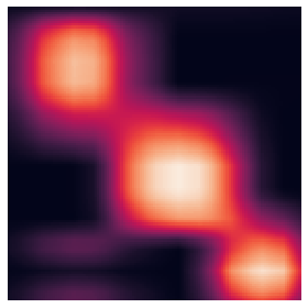
(a)

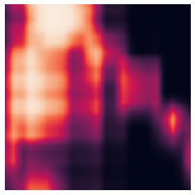
(b)

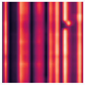
(c)

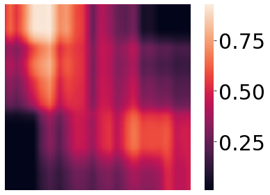
(d)

Figure 2: Visualization of attention matrices. (a) single-mode attention matrix of ‘channel-only’ token, (b)–(d) coupled-mode attention matrices of ‘channel-hyper-edge’, ‘order-channel-body joint’ and ‘channel-temporal block’ tokens, respectively.

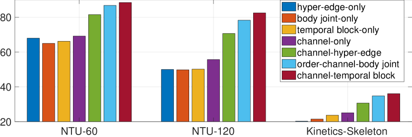
Figure 3: Evaluations of different single-mode (baseline) and coupled-mode tokens. We use a 3rd-order HoT with a standard Transformer, but we replace the scaled dot-product attention with coupled-mode tokens and coupled-mode attention.

Discussion on coupled-mode attention. Fig. 2 shows the visualization of some attention matrices in our 3Mformer, which show diagonal and/or vertical patterns that are consistent with the patterns of the attention matrices found in standard Transformer trained on sequences, e.g., for natural language processing tasks [49, 28]. We also notice that the coupled-mode attention, e.g., ‘channel-temporal block’ captures much richer information compared to single mode attention, e.g., ‘channel-only’. Our coupled-mode attention can be applied to different orders of tensor representations through simple matricization.

Discussion on model variants. To show the effectiveness of the proposed MP and TP module, firstly, we compare TP only and MP only with the baseline (No MP or TP module). We use the TP module followed by an FC layer instead of MP as in TP$\rightarrow$MP, where the FC layer takes the output from TP ($\mathbb{R}^{d^{\prime}N}$) and produces a vector in $\mathbb{R}^{3d^{\prime}J}$, passed to the classifier. Similarly, for MP only, we use the MP module followed by an average pooling layer instead of TP as in MP$\rightarrow$TP, where the average layer takes output from MP ($\mathbb{R}^{3d^{\prime}J\times\tau}$) and generates a vector in $\mathbb{R}^{3d^{\prime}J}$ (pool along $\tau$ blocks), passed to the classifier. Table 2 shows the results. With just the TP module, we outperform the baseline by 1.3% on average. With only the MP module, we outperform the baseline by 2.34% on average. These comparisons show that (i) CmSA in MP and TP are efficient for better performance (ii) MP performs better than TP which shows that ‘channel-temporal block’ token contains richer information than ‘channel-hyper-edge’ token. We also notice that MP$\rightarrow$TP slightly outperforms TP$\rightarrow$MP by $\sim$ 1%, and the main reason is that MP$\rightarrow$TP has coupled-mode tokens ‘channel-temporal block’ and ‘order-channel-joint’ which attend 4 modes, whereas TP$\rightarrow$MP has ‘channel-hyper-edge’ and ‘channel-only’ tokens which attend only 2 modes. Fig. 3 shows a comparison of different coupled-mode tokens on 3 benchmark datasets. This also suggests that one should firstly perform attention with coupled-mode ‘channel-block’ tokens, followed by weighted pooling along the hyper-edge mode, followed by attention with coupled-mode ‘order-channel-body joint’ and finalised by block-temporal pooling. Finally, with 2-branch (3Mformer), we further boost the performance by 2–4%, which shows that MP$\rightarrow$TP and TP$\rightarrow$MP are complementary branches. Below we use 2-branch (3Mformer) in the experiments (as in Fig. 1).

Comparison of pooling in TP. As shown in Table 3, average pooling (avg-pool) achieves similar performance (within $\sim$ 0.5% difference) as maximum pooling (max-pool), second-order pooling (attn-pool) outperforms average and maximum pooling by $\sim$ 1–2% and third-order pooling (tri-pool) outperforms second-order pooling by $\sim$ 1%. Interestingly, rank pooling (rank-pool) achieves the best performance. We think it is reasonable as rank pooling strives to enforce the temporal order in the feature space to be preserved, e.g., it forces network to always preserve temporal progression of actions over time. With multiple attention modules, orderless statistics such as second- or third-order pooling may be too general.

5.4 Comparisons with the State of the Arts

We compare our model with recent state-of-the-art methods. On the NTU-60 (Tab. 3), we obtain the top-1 accuracies of the two evaluation protocols during test stage. The methods in comparisons include popular graph-based [64, 30, 44, 37, 31] and hypergraph-based models [15, 62, 79, 17]. Our 3rd-order model outperforms all graph-based methods, and also outperforms existing hypergraph-based models such as Selective-HCN and SD-HGCN by 0.45% and 0.35% on average on X-Sub and X-View respectively. With 3Mformer for the fusion of multi-order features, our model further boosts the performance by $\sim$ 3% and 1.5% on the two protocols.

It can be seen from Tab. 3 on NTU-60 that although some learned graph-based methods such as AS-GCN and 2S-AGCN can also capture the dependencies between human body joints, they only consider the pairwise relationship between body joints, which is the second-order interaction, and ignore the higher-order interaction between multiple body joints in form of hyper-edges, which may lose sensitivity to important groups of body joints. Our proposed 3Mformer achieves better performance by constructing a hypergraph from 2D/3D body joints as nodes for action recognition, thus capturing higher-order interactions of body joints to further improve the performance. Note that even with the average pooling, our model still achieves competitive results compared to its counterparts.

For the NTU-120 dataset (Tab. 3), we obtain the top-1 performance on X-Sub and X-Set protocols. Our 2nd-order HoT alone outperforms graph-based models by 2–2.4% on average. For example, we outperform recent Shift-GCN by 0.3% and 0.7% on X-Sub and X-Set respectively. Moreover, our 3rd-order HoT alone outperforms SD-HGCN by 0.5% and 1.5% respectively on X-Sub and X-Set. With the 3Mformer for the fusion of multi-order feature maps, we obtain the new state-of-the-art results. Notice that our 3Mformer yields 92.0% / 93.8% on NTU-120 while [38] yields 80.5% / 81.7% as we explore the fusion of multiple orders of hyperedges and several coupled-token types capturing easy-to-complex dynamics of varying joint groups.

As videos from the Kinetics dataset are processed by the OpenPose, the skeletons in the Kinetics-Skeleton dataset have defects which adversely affect the performance of the model. We show both top-1 and top-5 performance in Table 3 to better reflect the performance of our 3Mformer. ST-GCN is the first method based on GCN, our 2nd-order HoT alone achieves very competitive results compared to the very recent NAS-GCN and Sym-GNN. The 3rd-order HoT alone outperforms Hyper-GNN, SD-HGCN and Selective-HCN by 3.4%, 3.1% and 2.9% respectively for top-1 accuracies. Moreover, fusing multi-order feature maps from multiple orders of hyper-edges via 3Mformer gives us the best performance on Kinetics-Skeleton with 48.3% for top-1, the new state-of-the-art result.

Table 4: Experimental results on Northwestern-UCLA.

	Shift-GCN [6]	CTR-GCN [4]	InfoGCN [9]	2nd-order	3rd-order	3Mformer
	(CVPR’20)	(ICCV’21)	(CVPR’22)	only (ours)	only (ours)	(ours)
acc.(%)	94.6	96.5	97.0	96.5	97.2	97.8

Table 4 shows results on the Northwestern-UCLA dataset. Our 3Mformer is also effective on this dataset–it outperforms the current state-of-the-art InfoGCN by 0.8%.

6 Conclusions

In this paper, we model the skeleton data as hypergraph to capture higher-order information formed between groups of human body joints of orders $1,...,r$. We use Higher-order Transformer (HoT) to learn higher-order information on hypergraphs of $r$-order formed over 2D/3D human body joints. We also introduce a novel Multi-order Multi-mode Transformer (3Mformer) for the fusion of multi-order feature representations. Our end-to-end trainable 3Mformer outperforms state-of-the-art graph- and hypergraph-based models by a large margin on several benchmarks.

Acknowledgements.

LW is supported by the Data61/ CSIRO PhD Scholarship. PK is in part funded by CSIRO’s Machine Learning and Artificial Intelligence Future Science Platform (MLAI FSP) Spatiotemporal Activity.

3Mformer: Multi-order Multi-mode Transformer
for Skeletal Action Recognition
– Supplementary Material –

Lei Wang^$\dagger,\S$  Piotr Koniusz^{$*,\S,\dagger$
†}Australian National University, ^§Data61$\varheartsuit$CSIRO
^§firstname.lastname@data61.csiro.au

Appendix A Visualization of 3Mformer

Fig. 4 shows the visualization of our 3Mformer. The green and orange blocks denote the Multi-order Pooling (MP) and the Temporal block Pooling (TP) respectively, which are two basic building blocks that can be stacked to form our 3Mformer. More precisely, our 3Mformer consists of two branches: (i) MP followed by TP (denoted MP $\rightarrow$ TP, Fig. 4(a)) and (ii) TP followed by MP (denoted TP $\rightarrow$ MP, Fig. 4(b)).

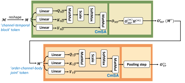
(a) Single-branch: MP followed by TP (denoted MP$\rightarrow$TP).

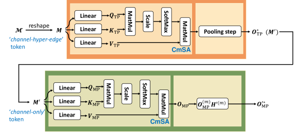
(b) Single-branch: TP followed by MP (denoted TP$\rightarrow$MP).

Figure 4: Visualization of 3Mformer which is a two- branch model: (a) MP$\rightarrow$TP and (b) TP$\rightarrow$MP. Green and orange blocks are Multi-order Pooling (MP) module and Temporal block Pooling (TP) module, respectively. $(m)$ inside the MP module denotes the order $m\in\mathcal{I}_{r}$ of hyper-edges. These two modules (MP and TP) are the basic building blocks which are further stacked to form our 3Mformer. Each module (MP or TP) uses a specific coupled-mode token through matricization (we use reshape for simplicity), e.g., ‘channel-temporal block’, ‘order-channel-body joint’, ‘channel-hyper-edge (any order)’ or ‘channel-only’, and the Coupled-mode Self-Attention (CmSA) is used to explore the coupled-mode relationships inside the coupled-mode tokens. We also form our multi-head CmSA as in standard Transformer (where the CmSA module repeats its computations multiple times in parallel and the attention module splits the query, key and value, each split is independently passed through a separate head and later combined together to produce the final coupled-mode attention score). We omit the multi-head visualization for simplicity and better visualization purposes.

Appendix B Skeletal Graph and Hypergraph

Skeletal Graph [64]. Let $G\!=\!({V},{E})$ be a skeletal graph with the vertex set ${V}$ of nodes (body joints) $\{v_{1},...,v_{J}\}$, and ${E}$ be edges (bones) of the graph, and ${E}$ consists of ${E}_{S}$ and ${E}_{T}$. The subset ${E}_{S}\!=\!\{(v_{it},v_{jt}):i,j\!\in\!\mathcal{I}_{J}\text{ and }t\!\in\!\mathcal{I}_{T}\}$ represents that at time step $t$, each pair of joints $(v_{it},v_{jt})$ corresponding to skeletal connectivity diagram is connected; whereas ${E}_{T}\!=\!\{(v_{it},v_{i(t+1)}):i\!\in\!\mathcal{I}_{J}\text{ and }t\!\in\!\mathcal{I}_{T}\}$ forms the connection of the same joint across time. The set of joints and edges together form the skeleton graph. If two body joints are connected by an edge, the corresponding element in the incidence matrix ${\bf H}$ is equal to 1, otherwise it is equal to 0, and the adjacency matrix ${\bf A}={\bf H}^{T}{\bf H}-2\mathbf{I}$ (where I is the identity matrix). The update rule of a common GCN model at time step $t$ is defined as:

$${\bf X}_{t}^{(l+1)}\!=\!\sigma\big{(}\widetilde{\bf D}^{-\frac{1}{2}}\widetilde{\bf A}\widetilde{\bf D}^{-\frac{1}{2}}{\bf X}_{t}^{(l)}\bm{\Theta}^{(l)}\big{)},$$ (11)

where $\sigma(\cdot)$ is a non-linearity, $\widetilde{\bf D}$ is the graph degree matrix, ${\bf X}_{t}^{(l)}$ is the input data of the convolutional layer $l$ at the time step $t$ and $\bm{\Theta}^{(l)}$ is the learnable parameters of layer $l$. $\widetilde{\bf A}\!=\!{\bf A}+{\bf I}$ is a normalized graph adjacency matrix.

The tensor representation of graph data can be given by ${\bf X}\!\in\!\mathbb{R}^{J^{2}\!\times\!d}$ where $d$ is the feature channel dimension.

Skeletal Hypergraph [35, 15]. Hypergraph captures complex higher-order relationships by hyper-edges that connect more than two nodes (body joints). Each hyper-edge is a subset of all nodes. Let $G_{h}\!=\!({V}_{h},{E}_{h},{W}_{h})$ where ${V}_{h}$, ${E}_{h}$ and ${W}_{h}$ denote respectively the set of body joints, hyper-edges and the weights of hyper-edges. Given $v\!\in\!{V}_{h}$ and $e\!\in\!{E}_{h}$, the elements in the incidence matrix ${\bf H}_{h}$ of the skeleton hypergraph are defined as ${H}_{h,v,e}=1$, or simply put $h(v,e)=1$, if vertex $v$ is part of edge $e$, 0 otherwise. The degree of node/body joint $v\!\in\!{V}_{h}$ is the number of hyper-edges passing through the node, which is defined as:

$$d(v)\!=\!\sum_{e\in{E}_{h}}w(e)h(v,e),$$ (12)

where $w(e)$ is the weight of hyper-edge $e$. The degree of hyper-edge $e\in{E}_{h}$ is the number of nodes (body joints) contained in the hyper-edge $e$ that satisfies:

$$\delta(e)\!=\!\sum_{v\in{V}_{h}}h(v,e).$$ (13)

Moreover, let ${\bf D}_{v}$ and ${\bf D}_{e}$ be the diagonal matrices of node degrees $d(v)$ and the hyper-edge degrees $\delta(e)$ respectively. Let ${\bf W}$ denote the diagonal matrix of the hyper-edge weights (initially the weights of all hyper-edges are set to 1). Then the update rule of the Hypergraph Convolutional Network at the time step $t$ is given by:

$${\bf X}_{t}^{(l+1)}\!=\!\sigma\big{(}{\bf D}_{v}^{\frac{1}{2}}{\bf H}_{h}{\bf W}{\bf D}_{e}^{-1}{\bf H}_{h}^{\top}{\bf D}_{v}^{\frac{1}{2}}{\bf X}_{t}^{(l)}\bm{\Theta}^{(l)}\big{)},$$ (14)

where $\bm{\Theta}^{(l)}$ are learnable parameters for layer $l$.

Appendix C Skeleton Data Preprocessing

Before passing the skeleton sequences into MLP, we first normalize each body joint w.r.t. to the torso joint ${\bf v}_{f,c}$:

$${\bf v}^{\prime}_{f,i}\!=\!{\bf v}_{f,i}\!-\!{\bf v}_{f,c},$$ (15)

where $f$ and $i$ are the index of video frame and human body joint respectively. After that, we further normalize each joint coordinate into [-1, 1] range:

$$\hat{{\bf v}}_{f,i}[j]=\frac{{\bf v}^{\prime}_{f,i}[j]}{\text{max}([\text{abs}({\bf v}^{\prime}_{f,i}[j])]_{f\in{\mathcal{I}_{\tau}},i\in\mathcal{I}_{J}})},$$ (16)

where $j$ is for selection of the $x$, $y$ and $z$ axes, $\tau$ is the number of frames and $J$ is the number of 3D body joints per frame.

For the skeleton sequences that have more than one performing subject, (i) we normalize each skeleton separately, and each skeleton is passed to MLP for learning the temporal dynamics, and (ii) for the output features per skeleton from MLP, we pass them separately to the block-temporal HoT, e.g., two skeletons from a given video sequence will have two outputs obtained from the the block-temporal HoT, and we aggregate the outputs through average pooling before passing our 3Mformer.

Appendix D Additional Results and Discussions

D.1 Ablations of MP

We choose average pooling (avg-pool) and max-pooling (max-pool) for hyper-edge features in comparison to our learned weighted pooling (wei-pool), and the comparisons are given in Table 5. As shown in the table, our learned weighted pooling (wei-pool) consistently achieves the best performance on all 3 datasets.

Table 5: Ablations of different pooling methods in MP.

Pooling	NTU-60		NTU-120		Kinetics-Skel.
	X-Sub	X-View	X-Sub	X-Set	Top-1 acc.
avg-pool	91.3	96.8	86.5	89.0	41.9
max-pool	92.7	98.0	88.5	91.0	43.8
wei-pool (ours)	94.8	98.7	92.0	93.8	48.3

D.2 Learning the short-term temporal patterns

A block of $T$ neighbor frames are passed to the MLP unit to capture the short-term temporal patterns. The whole sequence consists of $\tau$ such blocks, each passed separately through the MLP unit (and each joint $1,...,J$). Thus, the MLP only mixes the information from $1,...,T$ frames of a given block/body joint $j$ and captures short-term relations (within-block) of a given 3D body joint (in contrast to between-block relations). The MLP unit input size is $3T$; 3 due to 3D coordinate). The $\text{MLP}\!:\!\mathbb{R}^{3T}\!\rightarrow\!\mathbb{R}^{d}$ contains: FC ($3T\!\rightarrow\!6T$), ReLU, FC ($6T\!\rightarrow\!9T$), ReLU, Dropout, FC ($9T\!\rightarrow\!d$). $J$ body joints and $\tau$ blocks are treated as the batch dimension. Feature output size $d$: 100, 150, 420 on NTU-60, NTU-120, Kinetics-Skeleton.

D.3 Why 3Mformer works and when does it fail?

Our method works well as it (i) uses skeletal hypergraphs of various orders to learn the interaction of varying size groups of skeletal joints (as opposed to typical skeleton graph physical connectivity), (ii) fuses groups multiple orders by 3Mformer by several coupled-token types via two basic building blocks (MP & TP) that learn various aspects of higher-order motion dynamics. Multiple-order hyperedges are more resistant to noise (e.g., Kinetics-Skeleton is noisy due to the pose estimation errors), if one body joint is noisy (but the rest is stable). We inject Gaussian noise into 3D ankle joints, vary noise amplitude, and we show the experimental results in Table 6. As shown in the table, our 3Mformer copes with noise better than ST-GCN.

Table 6: Comparisons of robustness w.r.t. Gaussian noise.

	original	$\times$ 1	$\times$ 1.5	$\times$ 2
ST-GCN	81.5	74.9 ($\downarrow$6.6)	69.2 ($\downarrow$12.3)	50.1 ($\downarrow$31.4)
3Mformer	94.8	91.9 ($\downarrow$2.9)	89.5 ($\downarrow$5.3)	86.8 ($\downarrow$8.0)

Our method may underperform if (i) the backbone encoder cannot efficiently produce higher-order features (ii) the number of skeletal joints are very large (the number of hyper-edge features would be very large) (iii) when dataset is too small to learn high-order interactions (extra learnable parameters). For example, see the experimental results on MSRAction3D in Table 7.

We notice that small datasets may be not enough to train high-order models (Table 7). On key classic large datasets, NTU-60, NTU-120 and Kinetics-Skeleton, we do not observe any issue as human motions exhibit similar multi-joint dynamics for typical action classes. Perhaps some fine-grained unusual action classes could pose problems.

Table 7: Experimental results on MSRAction3D.

order	2	3	4
acc.(%)	73.82	63.64	55.27

D.4 Model Complexity

Table 8 shows the number of model parameters/FLOPs and NTU-60 accuracy. Our cost is moderate. 2S-AGCN (37.22 GFLOPs & 3.45M param.) yields 89.4% accuracy. Our ‘3rd-order’ uses 35.5 GFLOPs & 2.07M param. which is 2 GFLOPs & 1.37M param. less, yet we outperform 2S-AGC by 1.9%. NAS-GCN uses 40.4 GFLOPs/2.2M param. more compared to our 3Mformer: we beat NAS-GCN by 4.4%.

Table 8: A comparison of the number of model parameters and FLOPs on NTU-60.

	ST-GCN	2S-AGCN	NAS-GCN	2rd-order	3rd-order	3Mformer
				only (ours)	only (ours)	(ours)
Params (M)	3.14	3.45	6.57	1.15	2.07	4.37
FLOPs (G)	16.36	37.22	108.82	6.54	35.53	58.45
Acc. (%)	81.5	88.5	89.4	83.0	91.3	94.8

D.5 Limitation and Future Work

Despite the high accuracy of our model, there are still some limitations. Firstly, as we use $r$ branches of HoT, the number of parameters and computational cost are higher than existing methods. However, our method with single branch, e.g., 3rd-order HoT only, still achieves very competitive results compared to existing graph-, transformer- and hypergraph-based models for the same parameter scale on 3 benchmarks. Secondly, in this work, we only use HoT block to encode the temporal block feature representations. The more efficient way is to redesign HoT block so that it is able to encode both short-term and long-term spatio-temporal features to simplify the backbone encoder, i.e., without the need of MLP unit. Note that the design of our 3Mformer is independent of the backbone encoder. Our 3Mformer is especially suitable for tensorial data, e.g., higher-order feature representations. Our future work will focus on applying our Multi-order Multi-mode Transformer (3Mformer) to other computer vision tasks with tensorial data.

References

- [1] Hassan Akbari, Liangzhe Yuan, Rui Qian, Wei-Hong Chuang, Shih-Fu Chang, Yin Cui, and Boqing Gong. VATT: Transformers for multimodal self-supervised learning from raw video, audio and text. In A. Beygelzimer, Y. Dauphin, P. Liang, and J. Wortman Vaughan, editors, Advances in Neural Information Processing Systems, 2021.
- [2] Zhe Cao, Tomas Simon, Shih-En Wei, and Yaser Sheikh. Realtime multi-person 2d pose estimation using part affinity fields. In The IEEE Conference on Computer Vision and Pattern Recognition (CVPR), July 2017.
- [3] Chun-Fu Chen, Quanfu Fan, and Rameswar Panda. Crossvit: Cross-attention multi-scale vision transformer for image classification. CoRR, abs/2103.14899, 2021.
- [4] Yuxin Chen, Ziqi Zhang, Chunfeng Yuan, Bing Li, Ying Deng, and Weiming Hu. Channel-wise topology refinement graph convolution for skeleton-based action recognition. In Proceedings of the IEEE/CVF International Conference on Computer Vision, pages 13359–13368, 2021.
- [5] Ke Cheng, Yifan Zhang, Congqi Cao, Lei Shi, Jian Cheng, and Hanqing Lu. Decoupling gcn with dropgraph module for skeleton-based action recognition. In Andrea Vedaldi, Horst Bischof, Thomas Brox, and Jan-Michael Frahm, editors, Computer Vision – ECCV 2020, pages 536–553, Cham, 2020. Springer International Publishing.
- [6] Ke Cheng, Yifan Zhang, Xiangyu He, Weihan Chen, Jian Cheng, and Hanqing Lu. Skeleton-based action recognition with shift graph convolutional network. In Proceedings of the IEEE Conference on Computer Vision and Pattern Recognition (CVPR), 2020.
- [7] Yi-Bin Cheng, Xipeng Chen, Dongyu Zhang, and Liang Lin. Motion-transformer: Self-supervised pre-training for skeleton-based action recognition. In Proceedings of the 2nd ACM International Conference on Multimedia in Asia, MMAsia ’20, New York, NY, USA, 2021. Association for Computing Machinery.
- [8] Anoop Cherian, Piotr Koniusz, and Stephen Gould. Higher-order pooling of cnn features via kernel linearization for action recognition. In 2017 IEEE Winter Conference on Applications of Computer Vision (WACV), pages 130–138, 2017.
- [9] Hyung-gun Chi, Myoung Hoon Ha, Seunggeun Chi, Sang Wan Lee, Qixing Huang, and Karthik Ramani. Infogcn: Representation learning for human skeleton-based action recognition. In Proceedings of the IEEE/CVF Conference on Computer Vision and Pattern Recognition (CVPR), pages 20186–20196, June 2022.
- [10] Krzysztof Marcin Choromanski, Valerii Likhosherstov, David Dohan, Xingyou Song, Andreea Gane, Tamas Sarlos, Peter Hawkins, Jared Quincy Davis, Afroz Mohiuddin, Lukasz Kaiser, David Benjamin Belanger, Lucy J Colwell, and Adrian Weller. Rethinking attention with performers. In International Conference on Learning Representations, 2021.
- [11] Alexey Dosovitskiy, Lucas Beyer, Alexander Kolesnikov, Dirk Weissenborn, Xiaohua Zhai, Thomas Unterthiner, Mostafa Dehghani, Matthias Minderer, Georg Heigold, Sylvain Gelly, Jakob Uszkoreit, and Neil Houlsby. An image is worth 16x16 words: Transformers for image recognition at scale. In International Conference on Learning Representations, 2021.
- [12] Haodong Duan, Yue Zhao, Kai Chen, Dahua Lin, and Bo Dai. Revisiting skeleton-based action recognition. In Proceedings of the IEEE/CVF Conference on Computer Vision and Pattern Recognition (CVPR), pages 2969–2978, June 2022.
- [13] Basura Fernando, Efstratios Gavves, Jose Oramas Oramas M., Amir Ghodrati, and Tinne Tuytelaars. Rank pooling for action recognition. IEEE Trans. Pattern Anal. Mach. Intell., 39(4):773–787, apr 2017.
- [14] Rohit Girdhar and Deva Ramanan. Attentional pooling for action recognition. In NIPS, 2017.
- [15] Xiaoke Hao, Jie Li, Yingchun Guo, Tao Jiang, and Ming Yu. Hypergraph neural network for skeleton-based action recognition. IEEE Transactions on Image Processing, 30:2263–2275, 2021.
- [16] Ryota Hashiguchi and Toru Tamaki. Vision transformer with cross-attention by temporal shift for efficient action recognition, 2022.
- [17] Changxiang He, Chen Xiao, Shuting Liu, Xiaofei Qin, Ying Zhao, and Xuedian Zhang. Single-skeleton and dual-skeleton hypergraph convolution neural networks for skeleton-based action recognition. In Teddy Mantoro, Minho Lee, Media Anugerah Ayu, Kok Wai Wong, and Achmad Nizar Hidayanto, editors, Neural Information Processing, pages 15–27, Cham, 2021. Springer International Publishing.
- [18] Yujian Jiang, Zhaoneng Sun, Saisai Yu, Shuang Wang, and Yang Song. A graph skeleton transformer network for action recognition. Symmetry, 14(8), 2022.
- [19] Angelos Katharopoulos, Apoorv Vyas, Nikolaos Pappas, and François Fleuret. Transformers are RNNs: Fast autoregressive transformers with linear attention. In Hal Daumé III and Aarti Singh, editors, Proceedings of the 37th International Conference on Machine Learning, volume 119 of Proceedings of Machine Learning Research, pages 5156–5165. PMLR, 13–18 Jul 2020.
- [20] Will Kay, Joao Carreira, Karen Simonyan, Brian Zhang, Chloe Hillier, Sudheendra Vijayanarasimhan, Fabio Viola, Tim Green, Trevor Back, Paul Natsev, Mustafa Suleyman, and Andrew Zisserman. The kinetics human action video dataset, 2017.
- [21] Jinwoo Kim, Saeyoon Oh, and Seunghoon Hong. Transformers generalize deepsets and can be extended to graphs & hypergraphs. In A. Beygelzimer, Y. Dauphin, P. Liang, and J. Wortman Vaughan, editors, Advances in Neural Information Processing Systems, 2021.
- [22] Tae Soo Kim and Austin Reiter. Interpretable 3d human action analysis with temporal convolutional networks. In 2017 IEEE Conference on Computer Vision and Pattern Recognition Workshops (CVPRW), pages 1623–1631, 2017.
- [23] Jun Kong, Yuhang Bian, and Min Jiang. Mtt: Multi-scale temporal transformer for skeleton-based action recognition. IEEE Signal Processing Letters, 29:528–532, 2022.
- [24] Piotr Koniusz, Lei Wang, and Anoop Cherian. Tensor representations for action recognition. In IEEE Transactions on Pattern Analysis and Machine Intelligence. IEEE, 2020.
- [25] Piotr Koniusz, Lei Wang, and Ke Sun. High-order tensor pooling with attention for action recognition. arXiv, 2021.
- [26] Piotr Koniusz and Hongguang Zhang. Power normalizations in fine-grained image, few-shot image and graph classification. In IEEE Transactions on Pattern Analysis and Machine Intelligence. IEEE, 2020.
- [27] Matthew Korban and Xin Li. Ddgcn: A dynamic directed graph convolutional network for action recognition. In Andrea Vedaldi, Horst Bischof, Thomas Brox, and Jan-Michael Frahm, editors, Computer Vision – ECCV 2020, pages 761–776, Cham, 2020. Springer International Publishing.
- [28] Olga Kovaleva, Alexey Romanov, Anna Rogers, and Anna Rumshisky. Revealing the dark secrets of BERT. In Proceedings of the 2019 Conference on Empirical Methods in Natural Language Processing and the 9th International Joint Conference on Natural Language Processing (EMNLP-IJCNLP), pages 4365–4374, Hong Kong, China, Nov. 2019. Association for Computational Linguistics.
- [29] John Boaz Lee, Ryan Rossi, and Xiangnan Kong. Graph classification using structural attention. In Proceedings of the 24th ACM SIGKDD International Conference on Knowledge Discovery and Data Mining, KDD ’18, page 1666–1674, New York, NY, USA, 2018. Association for Computing Machinery.
- [30] Maosen Li, Siheng Chen, Xu Chen, Ya Zhang, Yanfeng Wang, and Qi Tian. Actional-structural graph convolutional networks for skeleton-based action recognition. In The IEEE Conference on Computer Vision and Pattern Recognition (CVPR), June 2019.
- [31] Maosen Li, Siheng Chen, Xu Chen, Ya Zhang, Yanfeng Wang, and Qi Tian. Symbiotic graph neural networks for 3d skeleton-based human action recognition and motion prediction. IEEE Transactions on Pattern Analysis and Machine Intelligence, 44(6):3316–3333, 2022.
- [32] Hezheng Lin, Xing Cheng, Xiangyu Wu, Fan Yang, Dong Shen, Zhongyuan Wang, Qing Song, and Wei Yuan. CAT: cross attention in vision transformer. CoRR, abs/2106.05786, 2021.
- [33] Tsung-Yu Lin, Subhransu Maji, and Piotr Koniusz. Second-order democratic aggregation. In ECCV, 2018.
- [34] Jun Liu, Amir Shahroudy, Mauricio Perez, Gang Wang, Ling-Yu Duan, and Alex C. Kot. Ntu rgb+d 120: A large-scale benchmark for 3d human activity understanding. IEEE Transactions on Pattern Analysis and Machine Intelligence, 2019.
- [35] Shengyuan Liu, Pei Lv, Yuzhen Zhang, Jie Fu, Junjin Cheng, Wanqing Li, Bing Zhou, and Mingliang Xu. Semi-dynamic hypergraph neural network for 3d pose estimation. In Christian Bessiere, editor, Proceedings of the Twenty-Ninth International Joint Conference on Artificial Intelligence, IJCAI-20, pages 782–788. International Joint Conferences on Artificial Intelligence Organization, 7 2020. Main track.
- [36] Ziyu Liu, Hongwen Zhang, Zhenghao Chen, Zhiyong Wang, and Wanli Ouyang. Disentangling and unifying graph convolutions for skeleton-based action recognition. In IEEE/CVF Conference on Computer Vision and Pattern Recognition (CVPR), June 2020.
- [37] Wei Peng, Xiaopeng Hong, Haoyu Chen, and Guoying Zhao. Learning graph convolutional network for skeleton-based human action recognition by neural searching. Proceedings of the AAAI Conference on Artificial Intelligence, 34(03):2669–2676, Apr. 2020.
- [38] Wei Peng, Jingang Shi, Tuomas Varanka, and Guoying Zhao. Rethinking the st-gcns for 3d skeleton-based human action recognition. Neurocomputing, 454:45–53, 2021.
- [39] Chiara Plizzari, Marco Cannici, and Matteo Matteucci. Skeleton-based action recognition via spatial and temporal transformer networks. Computer Vision and Image Understanding, 208-209:103219, 2021.
- [40] Zhenyue Qin, Yang Liu, Pan Ji, Dongwoo Kim, Lei Wang, Bob McKay, Saeed Anwar, and Tom Gedeon. Fusing higher-order features in graph neural networks for skeleton-based action recognition. IEEE TNNLS, 2022.
- [41] Saimunur Rahman, Piotr Koniusz, Lei Wang, Luping Zhou, Peyman Moghadam, and Changming Sun. Learning partial correlation based deep visual representation for image classification. In CVPR, 2023.
- [42] Kanchana Ranasinghe, Muzammal Naseer, Salman Khan, Fahad Shahbaz Khan, and Michael Ryoo. Self-supervised video transformer. In IEEE/CVF International Conference on Computer Vision and Pattern Recognition, June 2022.
- [43] Amir Shahroudy, Jun Liu, Tian-Tsong Ng, and Gang Wang. Ntu rgb+d: A large scale dataset for 3d human activity analysis. In IEEE Conference on Computer Vision and Pattern Recognition, June 2016.
- [44] Lei Shi, Yifan Zhang, Jian Cheng, and Hanqing Lu. Two-stream adaptive graph convolutional networks for skeleton-based action recognition. In CVPR, 2019.
- [45] Lei Shi, Yifan Zhang, Jian Cheng, and Hanqing Lu. Adasgn: Adapting joint number and model size for efficient skeleton-based action recognition. In Proceedings of the IEEE/CVF International Conference on Computer Vision (ICCV), pages 13413–13422, October 2021.
- [46] Chenyang Si, Wentao Chen, Wei Wang, Liang Wang, and Tieniu Tan. An attention enhanced graph convolutional lstm network for skeleton-based action recognition. In The IEEE Conference on Computer Vision and Pattern Recognition (CVPR), June 2019.
- [47] Yi-Fan Song, Zhang Zhang, Caifeng Shan, and Liang Wang. Constructing stronger and faster baselines for skeleton-based action recognition. IEEE Transactions on Pattern Analysis and Machine Intelligence, pages 1–1, 2022.
- [48] Zhan Tong, Yibing Song, Jue Wang, and Limin Wang. Videomae: Masked autoencoders are data-efficient learners for self-supervised video pre-training. CoRR, abs/2203.12602, 2022.
- [49] Ashish Vaswani, Noam Shazeer, Niki Parmar, Jakob Uszkoreit, Llion Jones, Aidan N Gomez, Ł ukasz Kaiser, and Illia Polosukhin. Attention is all you need. In I. Guyon, U. Von Luxburg, S. Bengio, H. Wallach, R. Fergus, S. Vishwanathan, and R. Garnett, editors, Advances in Neural Information Processing Systems, volume 30. Curran Associates, Inc., 2017.
- [50] Petar Veličković, Guillem Cucurull, Arantxa Casanova, Adriana Romero, Pietro Liò, and Yoshua Bengio. Graph attention networks. In International Conference on Learning Representations, 2018.
- [51] Jiang Wang, Xiaohan Nie, Yin Xia, Ying Wu, and Song-Chun Zhu. Cross-view action modeling, learning and recognition. In Proceedings of the IEEE conference on computer vision and pattern recognition, pages 2649–2656, 2014.
- [52] Lei Wang. Analysis and evaluation of Kinect-based action recognition algorithms. Master’s thesis, School of the Computer Science and Software Engineering, The University of Western Australia, 11 2017.
- [53] Lei Wang, Du Q. Huynh, and Piotr Koniusz. A comparative review of recent kinect-based action recognition algorithms. TIP, 2019.
- [54] Lei Wang, Du Q. Huynh, and Moussa Reda Mansour. Loss switching fusion with similarity search for video classification. ICIP, 2019.
- [55] Lei Wang and Piotr Koniusz. Self-Supervising Action Recognition by Statistical Moment and Subspace Descriptors, page 4324–4333. Association for Computing Machinery, New York, NY, USA, 2021.
- [56] Lei Wang and Piotr Koniusz. Temporal-viewpoint transportation plan for skeletal few-shot action recognition. In Proceedings of the Asian Conference on Computer Vision, pages 4176–4193, 2022.
- [57] Lei Wang and Piotr Koniusz. Uncertainty-dtw for time series and sequences. In Computer Vision–ECCV 2022: 17th European Conference, Tel Aviv, Israel, October 23–27, 2022, Proceedings, Part XXI, pages 176–195. Springer, 2022.
- [58] Lei Wang, Piotr Koniusz, and Du Q. Huynh. Hallucinating IDT descriptors and I3D optical flow features for action recognition with cnns. In ICCV, 2019.
- [59] Lei Wang, Jun Liu, and Piotr Koniusz. 3d skeleton-based few-shot action recognition with jeanie is not so naïve. arXiv preprint arXiv:2112.12668, 2021.
- [60] Qilong Wang, Zilin Gao, Jiangtao Xie, Wangmeng Zuo, and Peihua Li. Global gated mixture of second-order pooling for improving deep convolutional neural networks. In S. Bengio, H. Wallach, H. Larochelle, K. Grauman, N. Cesa-Bianchi, and R. Garnett, editors, Advances in Neural Information Processing Systems, volume 31. Curran Associates, Inc., 2018.
- [61] Chen Wei, Haoqi Fan, Saining Xie, Chao-Yuan Wu, Alan L. Yuille, and Christoph Feichtenhofer. Masked feature prediction for self-supervised visual pre-training. CoRR, abs/2112.09133, 2021.
- [62] Jinfeng Wei, Yunxin Wang, Mengli Guo, Pei Lv, Xiaoshan Yang, and Mingliang Xu. Dynamic hypergraph convolutional networks for skeleton-based action recognition. CoRR, abs/2112.10570, 2021.
- [63] Xi Wei, Tianzhu Zhang, Yan Li, Yongdong Zhang, and Feng Wu. Multi-modality cross attention network for image and sentence matching. In Proceedings of the IEEE/CVF Conference on Computer Vision and Pattern Recognition (CVPR), June 2020.
- [64] Sijie Yan, Yuanjun Xiong, and Dahua Lin. Spatial Temporal Graph Convolutional Networks for Skeleton-Based Action Recognition. In AAAI, 2018.
- [65] Han Zhang, Yonghong Song, and Yuanlin Zhang. Graph convolutional lstm model for skeleton-based action recognition. In 2019 IEEE International Conference on Multimedia and Expo (ICME), pages 412–417, 2019.
- [66] Jiani Zhang, Xingjian Shi, Junyuan Xie, Hao Ma, Irwin King, and Dit-Yan Yeung. Gaan: Gated attention networks for learning on large and spatiotemporal graphs. In Amir Globerson and Ricardo Silva, editors, UAI, pages 339–349. AUAI Press, 2018.
- [67] Pengfei Zhang, Cuiling Lan, Wenjun Zeng, Junliang Xing, Jianru Xue, and Nanning Zheng. Semantics-guided neural networks for efficient skeleton-based human action recognition. In IEEE/CVF Conference on Computer Vision and Pattern Recognition (CVPR), June 2020.
- [68] Shan Zhang, Dawei Luo, Lei Wang, and Piotr Koniusz. Few-shot object detection by second-order pooling. In ACCV, 2020.
- [69] Shan Zhang, Naila Murray, Lei Wang, and Piotr Koniusz. Time-reversed diffusion tensor transformer: A new tenet of few-shot object detection. In ECCV, 2022.
- [70] Shan Zhang, Lei Wang, Naila Murray, and Piotr Koniusz. Kernelized few-shot object detection with efficient integral aggregation. In CVPR, 2022.
- [71] Xikun Zhang, Chang Xu, and Dacheng Tao. Context aware graph convolution for skeleton-based action recognition. In IEEE/CVF Conference on Computer Vision and Pattern Recognition (CVPR), June 2020.
- [72] Yongkang Zhang, Jun Li, Guoming Wu, Han Zhang, Zhiping Shi, Zhaoxun Liu, and Zizhang Wu. Temporal transformer networks with self-supervision for action recognition. CoRR, abs/2112.07338, 2021.
- [73] Yuhan Zhang, Bo Wu, Wen Li, Lixin Duan, and Chuang Gan. Stst: Spatial-temporal specialized transformer for skeleton-based action recognition. In Proceedings of the 29th ACM International Conference on Multimedia, MM ’21, page 3229–3237, New York, NY, USA, 2021. Association for Computing Machinery.
- [74] Yifei Zhang, Hao Zhu, Zixing Song, Piotr Koniusz, and Irwin King. COSTA: Covariance-preserving feature augmentation for graph contrastive learning. In KDD, 2022.
- [75] Yifei Zhang, Hao Zhu, Zixing Song, Piotr Koniusz, and Irwin King. Spectral feature augmentation for graph contrastive learning and beyond. In AAAI, 2023.
- [76] Hao Zhu and Piotr Koniusz. Simple spectral graph convolution. In ICLR, 2021.
- [77] Hao Zhu and Piotr Koniusz. Generalized laplacian eigenmaps. In NeurIPS, 2022.
- [78] Hao Zhu, Ke Sun, and Piotr Koniusz. Contrastive laplacian eigenmaps. In NeurIPS, 2021.
- [79] Yiran Zhu, Guangji Huang, Xing Xu, Yanli Ji, and Fumin Shen. Selective hypergraph convolutional networks for skeleton-based action recognition. In Proceedings of the 2022 International Conference on Multimedia Retrieval, ICMR ’22, page 518–526, New York, NY, USA, 2022. Association for Computing Machinery.
- [80] Gao Zilin, Xie Jiangtao, Wang Qilong, and Li Peihua. Global second-order pooling convolutional networks. In The IEEE Conference on Computer Vision and Pattern Recognition (CVPR), 2019.