Verifying Properties of Tsetlin Machines

Abstract

Tsetlin Machines (TsMs) are a promising and interpretable machine learning method which can be applied for various classification tasks. We present an exact encoding of TsMs into propositional logic and formally verify properties of TsMs using a SAT solver. In particular, we introduce in this work a notion of similarity of machine learning models and apply our notion to check for similarity of TsMs. We also consider notions of robustness and equivalence from the literature and adapt them for TsMs. Then, we show the correctness of our encoding and provide results for the properties: adversarial robustness, equivalence, and similarity of TsMs. In our experiments, we employ the MNIST and IMDB datasets for (respectively) image and sentiment classification. We discuss the results for verifying robustness obtained with TsMs with those in the literature obtained with Binarized Neural Networks on MNIST.

I Introduction

Tsetlin Machines (TsMs) [6] have recently demonstrated competitive accuracy, learning speed, low memory, and low energy footprint on several tasks, including tasks related to image classification [5, 14], natural language classification [21, 13, 3, 20], speech processing [10], spanning tabular data [1, 18], and regression tasks. TsMs are less prone to overfitting, as the training algorithm does not rely on minimising an error function. Instead, the algorithm uses frequent pattern mining and resource allocation principles to extract common patterns from the data.

Unlike the intertwined nature of pattern representation in neural networks, TsMs decompose problems into self-contained patterns that are expressed using monomials. That is, a multiplication of Boolean variables (or their negations), also called conjunctive clauses [6]. The self-contained patterns are combined to form classification decision through a majority vote, akin to logistic regression, however, with binary weights and a unit step output function. The monomials are used to build an output formula for TsMs. This formula provides an interpretable explanation of the model, which is useful to check if decisions are unfair, biased, or erroneous.

Example 1.

TsMs trained for sentiment analysis can create monomials such as [21]:

$$C^{+}(1) ={\sf truly}\cdot\overline{{\sf depressive}}\cdot\overline{{\sf long}}\cdot\overline{{\sf worst}}$$

$$C^{+}(2) =\overline{{\sf boring}}\cdot\overline{{\sf worst}}\cdot\overline{{\sf long}}\cdot\overline{{\sf pretentious}}$$

$$C^{-}(1) =\overline{{\sf excellent}}\cdot\overline{{\sf good}}\cdot\overline{{\sf like}}$$

$$C^{-}(2) =\overline{{\sf friendly}}\cdot\overline{{\sf charming}}\cdot\overline{{\sf fascinating}}$$

where $C^{+}(i)$ monomials are associated with positive sentiment and $C^{-}(i)$ monomials are negative. Inputs that trigger more monomials of a certain class will be classified as such. E.g., the comment “How truly, friendly, charming, and cordial is this unpretentious old serial” triggers both positive monomials of our toy example but only one negative, namely $C^{-}(1)$, and, by majority vote, it is classified as positive.

However, current machine learning approaches (explainable or not) may not be robust, meaning that small amounts of noise can make the model change the classification in unexpected and uncontrolled ways [16]. Non-robustness poses a real threat to the applicability of machine learning models. This is of critical consideration because adversarial attacks can weaken malware detection systems [8], alter commands entered by users through speech recognition software [19], pose a security threat for systems that use computer vision [23], such as self-driving cars, identity verification, medical-diagnosis, among others.

The potential lack of robustness of machine learning models has driven the research community into finding strategies to formally verify properties of such models. A desired robustness property (e.g., if the model would change the classification of a binary image if $k$ bits are flipped) is not met if we are able to find a counterexample for it. The problem is that such counterexamples are spread in a vast space of possible examples. The first strategy to formally verify the robustness of machine learning models via an exact encoding into a SAT problem is the one proposed by Narodytska et al. for binarized (deep) neural networks (BNNs) [12]. This formal logic-based verification approach gives solid guarantees that corruption will not change the classification (up to a predefined upper bound on the number of corrupted bits, we are 100% sure the classification will not change for a given verified dataset). This is not possible using pure machine learning based approaches. The authors present an exact encoding of a trained BNN into propositional logic. Once the robustness property is converted into a SAT problem, one can formally verify robustness using SAT solvers.

Our work is the first work that investigates robustness properties of TsMs using a SAT solver. Checking robustness via an exact encoding provides formal guarantees of the model to adversarial attacks. One can also study relations between meta-parameters of the model, compare different learned models, and detect classification errors. In particular, we provide an exact encoding into propositional logic that captures the classification of TsMs and leverage the capability of modern automated reasoning procedures to explore large search spaces and check for similarity between models.

In this work we check adversarial robustness, equivalence, and similarity. In the mentioned work [12], adversarial robustness is tested for BNNs but they do not provide results for equivalence and do not consider similarity. Our results indicate that TsMs provide competitive accuracy results and robustness results when compared to BNNs on tested datasets. We test the mentioned properties of TsMs using the MNIST [4] and the IMDB [11] datasets. The results are promising, however, the time consumed for checking robustness increases exponentially on the number of parameters in the worst case (this is an unavoidable shortcoming of formal verification based on SAT solvers since the SAT problem is an NP-hard problem), which challenges the scalability of the approach.

In the following, we first present, in Section II, the TsM learning approach and provide basic definitions that are needed to understand the rational behind the encoding. In Section III, we explain how to encode a TsM in a propositional formula and we show the method used to check for robustness, equivalence, and similarity. In Section IV, we empirically evaluate the approach and we conclude in Section V. The full version of our paper, with omitted proofs and an appendix about TsMs, is available at https://arxiv.org/abs/2303.14464.

II Definitions and notations

We provide basic notions of propositional logic and the TsM learning and classification algorithm required to understand how to prove properties of TsMs.

II-A Propositional Logic and Vectors

We use standard propositional logic formulas to define the SAT encoding of TsMs and the formulas for checking robustness. In our notation, we write ${\sf V}$ for a finite set of Boolean variables, used to construct our propositional formulas. Every variable in ${\sf V}$ is a propositional formula over ${\sf V}$. We omit ‘over ${\sf V}$’ since all propositional formulas we speak of are formulated using (a subset of) symbols from ${\sf V}$. For propositional formulas $\phi$ and $\psi$, the expressions $(\phi\wedge\psi)$ and $(\phi\vee\psi)$ are propositional formulas, the conjunction and the disjunction of $\phi,\psi$, respectively. Also, if $\phi$ is a propositional formula then $\neg\phi$ (the negation of $\phi$) is a propositional formula. The semantics is given by interpretations, as usual in propositional logic. They map each variable in ${\sf V}$ to either “true” ($1$) or “false” ($0$). For a formula $\phi$, we write $\phi_{[\vec{x}\rightarrow{\mathcal{I}}]}$ for the result of replacing each $x\in\vec{x}$ in $\phi$ by $\mathcal{I}(x)$.

TsMs are trained on classified binary vectors in the $n$-dimensional space, with $n<|\mathsf{V}|$. In our work, it is useful to talk about interpretations and their vector representation interchangeably. The mapping from interpretations to vectors is defined as follows. We assume a total order on the elements of $\mathsf{V}$. Given an interpretation $\mathcal{I}$ over $\mathsf{V}$, the vector representation of $\mathcal{I}$ in the $n$-dimensional space is of the form $[\mathcal{I}(x_{1}),\ldots,\mathcal{I}(x_{n})]$ (note that ${\sf V}$ can have more variables). Also, we write $\mathcal{I}[i]$ for the value $\mathcal{I}(x_{i})$ of the $i$-th variable $x_{i}$. A (binary) dataset is a set of elements of the form $(\mathcal{I},y)$, where $y$ (the classification label of $\mathcal{I}$) is either $0$ or $1$ and $\mathcal{I}$ is an interpretation, treated as a vector in the $n$-dimensional space. The $n$-hamming distance of two interpretations $\mathcal{I}$ and $\mathcal{J}$ over $\mathsf{V}$, denoted $H_{n}(\mathcal{I},\mathcal{J})$, is the sum of differing values between $\mathcal{I}$ and $\mathcal{J}$.

II-B The Tsetlin Machine

We now present the main notions for the TsM algorithm (Algorithm 1). The algorithm is based on the notion of Tsetlin Automata (TA) [17]. A TA is a simple finite automaton that performs $2$ actions and updates the current state according to positive or negative feedback. We assume the initial state to be the exclude state that is closer to the center. TAs have no final states [17]. The shaded area in Figure 1 shows a TA with $4$ states. If a positive feedback is received, the automaton shifts to a state on the right and performs the action labelled in the current state, otherwise it shifts to a left state. The TsM algorithm uses a collection of TAs. Each single TA is represented by just an integer in memory and the TsM learning algorithm (explained later) modifies the value of the integer, based on its input. Each TA votes for a specific pattern, inclusion or exclusion of variables (the number of variables matches with the dimension of the TsM input vector).

An example of a set of TAs voting for a pattern is depicted in Figure 1. For binary classification, the TsM algorithm divides the set of $n$ TAs into two, denoted $C^{+}$ and $C^{-}$. The TAs in the set $C^{+}$ vote for a positive label of the input while the TAs in $C^{-}$ vote negatively. For $k\in\{+,-\}$, and $1\leq j\leq n/2$, we denote by $C^{k}(j)$ the pattern recognised by the $j$-th set of TAs belonging to group $C^{k}$. Each pattern $C^{k}(j)$ is represented as a monomial, that is a multiplication of Boolean variables or their negation. For a Boolean variable $x$ we denote its negation with $\overline{x}$, which is the same as $1-x$. In Figure 1, the monomial is $x_{1}\overline{x_{2}}$. Monomials can be represented as a conjunction of variables or their negation (e.g., the monomial $x_{1}\overline{x_{2}}$ corresponds to $x_{1}\wedge\neg x_{2}$). In previous works on TsMs (e.g., [6]), the authors have used sums and disjunctions interchangeably. However, in our work, it is useful to distinguish between the two representations because the sum of multiple non-zero monomials is counted using the sequential counters in Subsection III-A. That is, $1+1$ is counted as $2$, which is not the same as $1\vee 1$, evaluated to “true” (in symbols, $1$). It is possible to have a literal and its negation in a monomial. This happens when the training data has some kind of inconsistent information [22].

The procedure for training a TsM is given by Algorithm 1. It initialises $n$ (num. of monomials) teams of TAs (one for each variable $V$ and its negation) with $N$ states per action (Line 3). Then, for each training example (Line 5), it loops for every TA team and apply the respective feedback type in order to update the recognised pattern. The value computed in Line 7 is used to guide the randomised selection for the type of feedback to give to the TAs. The function ${\sf clip}$ is used to bound the sum between the interval $[-T,T]$. Finally, the algorithm returns the functions $C^{+},C^{-}$. We denote with $\mathcal{M}(S,V,n,N,T,s)$ the formula

$$\sum^{n/2}_{j=1}C^{-}(j)\geq\sum^{n/2}_{j=1}C^{+}(j)$$ (1)

built from the functions $C^{+},C^{-}$ returned by Algorithm 1 with $S$, $V$, $n$, $N$, $T$, and $s$ as input. We may omit $(S,V,n,N,T,s)$ if this is clear from the context and call a expression $\mathcal{M}$ in this format a TsM formula. Given an interpretation $\mathcal{I}$, we write $\mathcal{M}(\mathcal{I})=0$—meaning that the classification of $\mathcal{I}$ is negative—if the result of replacing each variable $x$ in the formula $\mathcal{M}$ by $\mathcal{I}(x)$ results in an expression where Equation 1 holds, otherwise $\mathcal{M}(\mathcal{I})=1$, that is, the classification of $\mathcal{I}$ is positive. We say that $\mathcal{I}$ is a positive (resp. negative) example for $\mathcal{M}$ if $\mathcal{M}(\mathcal{I})=1$ (resp. $\mathcal{M}(\mathcal{I})=0$).

Example 2.

Assume the TsM formula $\mathcal{M}$ is

$$x_{1}\overline{x_{2}}+\overline{x_{1}}x_{2}\geq x_{1}x_{2}+\overline{x_{1}}\ \overline{x_{2}}.$$

Then, e.g., $C^{-}(1)=x_{1}\overline{x_{2}}$, and $C^{+}(2)=\overline{x_{1}}\ \overline{x_{2}}$. If $\mathcal{I}(x_{1})=1$ and $\mathcal{I}(x_{2})=0$, after substituting the values in the formula, we have $1+0\geq 0+0$. So, the TsM classifies $\mathcal{I}$ as $0$. In symbols, $\mathcal{M}(\mathcal{I})=0$.

Each $C^{k}(j)$ is trained by receiving two feedback types given an input $\mathcal{I}$ with a classification label. In short, Feedback I is given to the TAs which vote for a classification matching with the label $y$ of the input $\mathcal{I}$. It aims at increasing the number of clauses that correctly evaluates a positive input to true. On the other hand, Feedback II is given to the TAs which do not vote for a classification matching with the label $y$ of the input $\mathcal{I}$. It aims at combating false positive output by increasing the discrimination power of the clauses. Granmo et al. proves theoretical guarantees regarding these feedbacks [6]. To perform multiclass classification on TsMs, one defines a TsM for each target class and decides the class by taking the TsM which classifies positively with the highest difference between positive and negative monomials.

Figure 1: 4 TAs, each of them vote for the inclusion or exclusion of their associated variables. Black states indicate the final position in each TA after training. The recognised pattern is $x_{1}\overline{x_{2}}$ as in function $C^{-}(1)$ in Example 2. A single TA voting for the inclusion of $x_{1}$ is depicted in the shaded area.

1:  Input: Training data $S$, features $V$, num. of monomials $n$, num. of states $N$, margin $T$, specificity $s$

2:  Output: the monomial functions $C^{+},C^{-}$

3:  $\mathcal{A}^{+},\mathcal{A}^{-}\leftarrow$ CreateTAs($n,N/2,V$)

4:  repeat

5:     $(\mathcal{I},y)\leftarrow$ GetTrainingExample($S$)

6:     $C^{+},C^{-}\leftarrow$ GetMonomials($\mathcal{A}^{+},\mathcal{A}^{-}$)

7:     $v\leftarrow{\sf clip}(\sum^{n/2}_{j=1}C^{-}(j)-\sum^{n/2}_{j=1}C^{+}(j),-T,T)$

8:     for $j\leftarrow 1,\ldots,n/2$ do

9:        if $y=1$ then

10:           if rand() $\leq(T-v)/(2T)$ then

11:              $\mathcal{A}^{+}\leftarrow$ GenerateTypeIFeedback($\mathcal{I},\mathcal{A}^{+}(j),s$)

12:              $\mathcal{A}^{-}\leftarrow$ GenerateTypeIIFeedback($\mathcal{I},\mathcal{A}^{-}(j)$)

13:           end if

14:        else

15:           if rand() $\leq(T+v)/(2T)$ then

16:              $\mathcal{A}^{+}\leftarrow$ GenerateTypeIIFeedback($\mathcal{I},\mathcal{A}^{+}(j)$)

17:              $\mathcal{A}^{-}\leftarrow$ GenerateTypeIFeedback($\mathcal{I},\mathcal{A}^{-}(j),s$)

18:           end if

19:        end if

20:     end for

21:  until StopCriteria($S,C^{+},C^{-}$)

22:  return $C^{+},C^{-}$

Algorithm 1 Tsetlin Machine

III Verifying Properties of TsMs

We first present an exact encoding of a TsM into propositional logic using sequential counters (Section III-A). We then use this encoding to define the properties adversarial robustness, equivalence, and similarity of TsMs.

III-A SAT Encoding

The encoding of TsMs into a propositional logic uses the translation of sequential counters into a logic formula [15]. Consider a cardinality constraint: $\sum^{\ell}_{i=1}l_{i}\geq K,$ where $l_{i}\in\{0,1\}$ and $K\in\mathbb{N}$. Then the cardinality constraint is encoded into a formula as follows:

$$\begin{split}&(l_{1}\leftrightarrow r_{1,1})\wedge(\neg r_{1,j})\wedge(r_{i,1}\leftrightarrow(l_{i}\vee r_{i-1,1}))\wedge\\ &(r_{i,j}\leftrightarrow((l_{i}\wedge r_{i-1,j-1})\vee r_{i-1,j}))\end{split}$$ (2)

where $i\in\{2,\ldots,\ell\}$ and $j\in\{2,\ldots,K\}$. Variables of the form $r_{i,j}$ are (fresh) auxiliary variables. Intuitively, this encoding computes cumulative sums. The variable $r_{\ell,K}$ is ‘true’ iff $\sum^{\ell}_{i=1}l_{i}$ is greater than or equal to $K$. For a cardinality constraint $c:=\sum^{\ell}_{i=1}l_{i}\geq K$, we denote by $\rho(c)$ the sequential counter encoding of $c$ into a formula (Eq. LABEL:eq:sc).

To express the TsM formula $\mathcal{M}=\sum^{n/2}_{j=1}C^{-}(j)\geq\sum^{n/2}_{j=1}C^{+}(j)$ in propositional logic, we define $\varrho(\mathcal{M})$ as:

$$\varrho(\mathcal{M}):=\bigwedge_{k\in\{+,-\}}\bigwedge_{j=1}^{n/2}(v_{k,j}\leftrightarrow C^{k}(j)^{\dagger})$$ (3)

$$\land\bigwedge_{k\in\{+,-\}}\rho(\sum^{n/2}_{j=1}v_{k,j}\geq n/2)$$ (4)

$$\land\bigwedge_{j=1}^{n/2}((r^{-}_{n/2,j}\rightarrow r^{+}_{n/2,j})\leftrightarrow o_{j})\wedge((\bigwedge_{j=1}^{n/2}o_{j})\leftrightarrow o)$$ (5)

where $v_{+,j}$ and $v_{-,j}$ are fresh propositional variables, with $1\leq j\leq n/2$, and $r^{k}_{n/2,j}$ are the auxiliary variables in the encoding given by the function $\rho(\cdot)$ for $k\in\{+,-\}$ (Eq. LABEL:eq:sc). We write $C^{k}(j)^{\dagger}$ for the result of converting a multiplication of variables into a conjunction of variables and replacing each variable of the form $\overline{x}$ by $\neg x$. Eq. 5 expresses that if $j$ monomials in $C^{-}$ are set to true, then at least $j$ monomials in $C^{+}$ are set to true. This information is stored in the variable $o$, which we call the output variable of the encoding $\varrho(\mathcal{M})$ (we use additional auxiliary variables $o_{j}$ for practical purposes, in particular, to reduce the size of the formula when converting it into CNF, which is the format required by most SAT solvers).

Example 3.

Consider the TsM formula $\mathcal{M}$ in Example 2. Then, $\varrho(\mathcal{M})$ is

$$(v_{-,1}\leftrightarrow(x_{1}\wedge\neg x_{2}))\wedge(v_{-,2}\leftrightarrow(\neg x_{1}\wedge x_{2})) \wedge$$

$$(v_{+,1}\leftrightarrow(x_{1}\wedge x_{2}))\wedge(v_{+,2}\leftrightarrow(\neg x_{1}\wedge\neg x_{2})) \wedge$$

$$\bigwedge_{i\in\{+,-\}}((v_{i,1}\leftrightarrow r^{i}_{1,1})\wedge(\neg r^{i}_{1,2})\wedge(r^{i}_{2,1}\leftrightarrow(v_{i,2}\vee r^{i}_{1,1})) \wedge$$

$$(r^{i}_{2,2}\leftrightarrow((v_{i,2}\wedge r^{i}_{1,1})\vee r^{i}_{1,2})))\wedge((r^{-}_{2,1}\rightarrow r^{+}_{2,1})\leftrightarrow o_{1}) \wedge$$

$$((r^{-}_{2,2}\rightarrow r^{+}_{2,2})\leftrightarrow o_{2})\wedge((o_{1}\wedge o_{2})\leftrightarrow o).$$

We are now ready to state Theorem 1, which essentially follows from the definition of $\varrho(\mathcal{M})$ and the correctness of the sequential counter encoding.

Theorem 1.

For a TsM formula $\mathcal{M}$ and an interpretation $\mathcal{I}$, $\mathcal{M}(\mathcal{I})=1$ iff $\varrho(\mathcal{M})_{[\vec{x}\rightarrow{\mathcal{I}}]}\wedge o$ is satisfiable.

Proof.

($\Rightarrow$) $\mathcal{M}(\mathcal{I})=1$ implies that the number of satisfied monomials in $C^{-}$ by $\mathcal{I}$ is at least equal to the number of satisfied monomials in $C^{+}$ by $\mathcal{I}$. We show that we can find an interpretation $\mathcal{J}$ that satisfies $\varrho(\mathcal{M})_{[\vec{x}\rightarrow{\mathcal{I}}]}\wedge o$. Initially we define $\mathcal{J}:=\mathcal{I}$. According to Eq. 3 and for $k\in\{+,-\}$, we constraint $\mathcal{J}$ so that $\mathcal{J}(v_{k,j})=1$ iff $C^{k}(j)$ is satisfied by $\mathcal{I}$. At this point, $\mathcal{J}$ satisfies the part of the encoding $\varrho(\mathcal{M})_{[\vec{x}\rightarrow{\mathcal{I}}]}$ in Eq. 3. Then, for $k\in\{+,-\}$, we count how many variables $v_{k,j}$ are set to true by $\mathcal{J}$, where $1\leq j\leq n/2$. Let $n_{k}$ be such number. We set $\mathcal{J}(r^{k}_{n/2,j})=1$ iff $j\leq n_{k}$ (the remaining variables of the form $r^{k}_{m,j}$ are set to true if the sum of the first $m$ variables $v_{k,j}$ is at least $j$). In this way, we satisfy Eq. 4 that corresponds to the second part of the encoding. Finally, Eq. 5 is already satisfied by the just built $\mathcal{J}$ because, since $\mathcal{M}(\mathcal{I})=1$, for every $1\leq j\leq n/2$, the rule $r^{-}_{n/2,j}\rightarrow r^{+}_{n/2,j}$ is satisfied, and so, adding $o$ as a conjunct in $\varrho(\mathcal{M})_{[\vec{x}\rightarrow{\mathcal{I}}]}\wedge o$ yields a satiafiable formula. ($\Leftarrow$) Let $\mathcal{J}$ be an interpretation that satisfies $\varrho(\mathcal{M})_{[\vec{x}\rightarrow{\mathcal{I}}]}\wedge o$. By Eq. 5, for all $1\leq j\leq n/2$, if $r^{-}_{n/2,j}$ is true then $r^{+}_{n/2,j}$ is true. This means that, in Eq. 4, if the sum of the $n/2$ variables $v_{-,j}$ is at least $j$ then this is so for the sum of the $n/2$ variables $v_{+,j}$. By Eq. 3 and the definition of $C^{k}(j)^{\dagger}$, this can only be if $\mathcal{M}(\mathcal{I})=1$. ∎

III-B Robustness

We use the encoding of TsMs in Subsection III-A to define and show correctness of adversarial robustness for TsMs.

Definition 1 (Adversarial Robustness).

Let $n$ be the dimension of the input of a TsM and let $\mathcal{M}$ be its formula. Such TsM is called $\epsilon$-robust for an interpretation $\mathcal{I}$ if there is no interpretation $\mathcal{J}$ such that $H_{n}(\mathcal{I},\mathcal{J})\leq\epsilon$ and $\mathcal{M}(\mathcal{I})\neq\mathcal{M}(\mathcal{J})$.

To check if a TsM is $\epsilon$-robust (Definition 1), we need to ensure that there are no $\epsilon$ bit flips of a given input vector $\mathcal{I}$ such that the classification on $\mathcal{I}$ of the TsM changes. We can explore the search space with the help of a SAT solver. To check for $\epsilon$-robustness, we call a SAT solver with the following formula ${\sf NotRob}(\mathcal{M},\mathcal{I},\epsilon)$ as input, where $\mathcal{M}$ is the TsM we would like to check robustness and $\mathcal{I}$ is an input for $\mathcal{M}$. The formula is satisfied if the TsM is not robust. That is, if we are able to find a combination of at most $\epsilon$ bit flips to apply to the input $\mathcal{I}$ such that the classification of the TsM changes.

We can check with a SAT solver if there is no assignment that satisfy ${\sf NotRob}(\mathcal{M},\mathcal{I},\epsilon)$, which means that the property of the TsM $\mathcal{M}$ being adversarially $\epsilon$-robust is satisfied. In the following, we write $\mathcal{M}_{\vec{x}}$ to make explicit that the $n$ variables $\vec{x}$ in $\mathcal{M}$ (the ones used to build the functions $C^{k}$ in $\varrho(\mathcal{M})$ (Eqs. 3-5)) are those $x_{j}$ in Eq. 7.

$${\sf NotRob}(\mathcal{M}_{\vec{x}},\mathcal{I},\epsilon):=\;\neg\rho(\sum_{j=1}^{n}l_{j}\geq\epsilon+1)\ \land$$ (6)

$$\bigwedge_{j=1}^{n}(x_{j}\leftrightarrow((\mathcal{I}[j]\lor l_{j})\land(\neg\mathcal{I}[j]\lor\neg l_{j})))\ \land$$ (7)

$$\varrho(\mathcal{M}_{\vec{x}})\land(\mathcal{M}_{\vec{x}}(\mathcal{I})\leftrightarrow\neg o)$$ (8)

In Eq. 6 we create new variables $l_{j}$ with $1\leq j\leq n$ and we specify with a sequential counter encoding that at most $\epsilon$ of such variables should have a ‘true’ truth value. Semantically, an $l_{j}$ is set to true if the truth value of $\mathcal{I}[i]$ should be flipped. In Eq. 7, we force the variables $x_{j}$ with $1\leq j\leq n$, that are used to define monomials in the TsM, to be the truth value of the flipped variable at position $i$ such that $x_{j}=\mathcal{I}[j]\oplus l_{j}$ (where $\oplus$ is the XOR operator). That is, $x_{i}$ is true if $\mathcal{I}[i]$ is true and the bit should not be flipped or if $\mathcal{I}[i]$ is false and the value should be flipped. In the other cases, the final value of the flipped variable is set to false. Finally, we add the constraint that the output of the TsM with the modified input (given by valuations of the variables $\vec{x}$) differs from the label of the original input. This means that the formula is satisfiable if the TsM is not $\epsilon$-robust for the input $\mathcal{I}$.

We show in Example 4 the not robust check for the TsM in Example 2 and an interpretation classified as negative.

Example 4.

Let $\mathcal{M}$ be the TsM in Example 2 and let $\epsilon=1$. We can check for the robustness of $\mathcal{M}$ with input the vector representation of an interpretation $\mathcal{I}$ with $\mathcal{I}[1]=0$ and $\mathcal{I}[2]=0$ (assume the dimension $n$ of the input of the TsM is $2$) and $\mathcal{M}(\mathcal{I})=0$ as follows:

$$\begin{aligned} \neg&((l_{1}\leftrightarrow t_{1,1})\land\neg t_{1,2}\land(t_{2,1}\leftrightarrow(l_{2}\lor t_{1,1}))&\land\\ &(t_{2,2}\leftrightarrow((l_{2}\land t_{1,1})\lor t_{1,2}))&\land\\ &(x_{1}\leftrightarrow((0\lor l_{1})\land(1\lor\neg l_{1})))&\land\\ &(x_{2}\leftrightarrow((0\lor l_{2})\land(1\lor\neg l_{2})))&\land\\ &\varrho(\mathcal{M}_{\vec{x}})\land(0\leftrightarrow\neg o).\end{aligned}$$ (9)

Theorem 2.

A TsM $\mathcal{M}$ is $\epsilon$-robust for $\mathcal{I}$ iff ${\sf NotRob}(\mathcal{M},\mathcal{I},\epsilon)$ is not satisfiable.

In a similar way, one can also check for a stronger property, denoted universal adversarial robustness. This property holds for a set of inputs if a TsM is robust to all adversarial perturbations (up to some threshold value) in a number of elements of this set. More specifically, if $S$ is the set of inputs considered, we would like to check if the TsM $\mathcal{M}$ classifies differently only an $\eta$-fraction of perturbed elements in $S$.

Definition 2 (Universal Adversarial Robustness).

Let $n$ be the dimension of the input of a TsM with formula $\mathcal{M}$. Then, $\mathcal{M}$ is $(\epsilon,\eta)$-robust for a set of classified inputs $S$ if it is $\epsilon$-robust for $\eta|S|$ or more classified inputs in $S$.

To check for this property, we check if a SAT solver does not find any assignment for the formula:

$${\sf{UniRob}}(\mathcal{M},S,\epsilon,\eta):=\;\rho(\sum_{i=1}^{|S|}c_{i}\geq\lfloor\eta|S|\rfloor)$$ (10)

$$\bigwedge_{(\mathcal{I}_{i},\mathcal{M}(\mathcal{I}_{i}))\in S}({\sf NotRob}(\mathcal{M},\mathcal{I}_{i},\epsilon)\leftrightarrow\neg c_{i})$$ (11)

In Eq. 9, each $c_{i}$ is a new variable that is set to true iff the $\epsilon$-robustness check with a specific example $\mathcal{I}_{i}$ has not passed. Then, in Eq. 11, we check whether the number of examples in which the non-robustness test failed passes a proportion of the set $S$ based on $\eta$.

Theorem 3.

A TsM $\mathcal{M}$ is $(\epsilon,\eta)$-robust for a set of inputs $S$ iff ${\sf{UniRob}}(\mathcal{M},S,\epsilon,\eta)$ is satisfiable.

III-C Equivalence and Similarity

Two TsMs are equivalent if they output the same class given the same input (Definition 3).

Definition 3.

Two TsMs $\mathcal{M}_{1}$ and $\mathcal{M}_{2}$ are equivalent if, for all interpretations $\mathcal{I}$ (as an input vector), $\mathcal{M}_{1}(\mathcal{I})=\mathcal{M}_{2}(\mathcal{I})$.

We can use the encoding $\varrho(\mathcal{M}_{i})$ for $1\leq i\leq 2$ presented in Section III-A to search for an input $\mathcal{I}$ that is classified differently by them. We assume a deterministic procedure for generating the variables in the encoding $\varrho(\mathcal{M}_{i})$, which guarantees that, if the dimension of the input vectors of the TsMs with formulas $\mathcal{M}_{1}$ and $\mathcal{M}_{2}$ are the same, then $\varrho(\mathcal{M}_{1})$ and $\varrho(\mathcal{M}_{2})$ are formulated using the same input variables $\vec{x}$.

Theorem 4.

Two TsMs $\mathcal{M}_{1}$ and $\mathcal{M}_{2}$ are equivalent iff $(\varrho(\mathcal{M}_{1})\wedge o^{1})\leftrightarrow(\varrho(\mathcal{M}_{2})\wedge o^{2})$ holds, where $o^{1},o^{2}$ are the output variables of $\varrho(\mathcal{M}_{1})$ and $\varrho(\mathcal{M}_{2})$, respectively.

One can imagine that a complete equivalence between machine learning models is difficult to achieve. It is therefore also interesting to consider the case in which TsMs are not equivalent but similar. We define similarity w.r.t. a set of inputs (and small perturbations) as follows.

Definition 4 (Similarity and Universal Similarity).

Let $n$ be the dimension of the input of TsMs with formulas $\mathcal{M}_{1}$ and $\mathcal{M}_{2}$. Then, $\mathcal{M}_{1}$ and $\mathcal{M}_{2}$ are $\epsilon$-similar for an interpretation $\mathcal{I}$ if they give the same classification result for $\mathcal{I}$ and all interpretations $\mathcal{J}$ such that $H_{n}(\mathcal{I},\mathcal{J})\leq\epsilon$. Moreover, $\mathcal{M}_{1}$ and $\mathcal{M}_{2}$ are $(\epsilon,\eta)$-similar for a set $S$ of inputs if they are $\epsilon$-similar for $\eta|S|$ or more inputs in $S$.

To check for similarity on an input $\mathcal{I}$, we check if a SAT solver does not find any assignment for the formula:

$${\sf NotSim}(\mathcal{M}_{1,\vec{x}},\mathcal{M}_{2,\vec{x}},\mathcal{I},\epsilon):=\;\neg\rho(\sum_{j=1}^{n}l_{j}\geq\epsilon+1)\ \land$$

$$\bigwedge_{j=1}^{n}(x_{j}\leftrightarrow((\mathcal{I}[j]\lor l_{j})\land(\neg\mathcal{I}[j]\lor\neg l_{j})))\ \land$$

$$\varrho(\mathcal{M}_{1,\vec{x}})\land\varrho(\mathcal{M}_{2,\vec{x}})\land(o^{1}\leftrightarrow\neg o^{2})$$

To check for universal similarity, we check if a SAT solver does not find any assignment for the formula:

$${\sf{UniSim}}(\mathcal{M}_{1,\vec{x}},\mathcal{M}_{2,\vec{x}},S,\epsilon,\eta):=\;\rho(\sum_{i=1}^{|S|}c_{i}\geq\lfloor\eta|S|\rfloor)$$

$$\bigwedge_{\mathcal{I}_{i}\in S}({\sf NotSim}(\mathcal{M}_{1,\vec{x}},\mathcal{M}_{2,\vec{x}},\mathcal{I}_{i},\epsilon)\leftrightarrow\neg c_{i})$$

The intuition for ${\sf{UniSim}}(\mathcal{M}_{1},\mathcal{M}_{2},S,\epsilon,\eta)$ is similar to the intuition for ${\sf{UniRob}}(\mathcal{M},S,\epsilon,\eta)$ except that here we check for two TsMs (with the same dimension).

Theorem 5.

TsMs $\mathcal{M}_{1}$ and $\mathcal{M}_{2}$ are (1) $\epsilon$-similar for an interpretation $\mathcal{I}$ iff ${\sf{NotSim}}(\mathcal{M}_{1},\mathcal{M}_{2},\mathcal{I},\epsilon)$ is unsatisfiable; and (2) $(\epsilon,\eta)$-similar for a set of inputs $S$ iff ${\sf{UniSim}}(\mathcal{M}_{1},\mathcal{M}_{2},S,\epsilon,\eta)$ is satisfiable.

IV Experiments and Results

We present the results of our experiments to verify properties of TsMs on the classical MNIST and IMDB datasets. In particular, we employ the formulas presented in Section III for checking adversarial robustness, equivalence, and similarity for image classification and sentiment analysis. We also perform some tests to compare TsMs and BNNs. To perform our experiments, we wrote the code in Python 3.8 and we used the Glucose SAT solver [2], which is the same SAT solver employed by Narodytska et al. in her mentioned work. We now describe the datasets used for training in more detail.

• The MNIST dataset consists of $60,000$ gray-scale $28\times 28$ images for training for the task of hand written single digits recognition and $10,000$ for testing. Images are binarized using an adaptive Gaussian thresholding procedure as proposed in [5].

• The IMDB dataset is a sentiment classification dataset consisting of $50,000$ movie reviews, where $25,000$ of the samples are used as training data and the other half as the testing set. The text is binarized using bags-of-words including the $5,000$ most frequent words.

We run all experiments on an AMD Ryzen 7 5800X CPU at 3.80GHz with 8 logical cores, Nvidia GeForce GTX 1070, and 32GB RAM. The code is available at https://github.com/bimalb58/Logical-Tsetlin-Machine-Robustness.

IV-A Training TsMs

TABLE I: TsMs models trained on MNIST.

	N	T	s	train acc	test acc	train time
1	500	25	10	99.20 %	97.41 %	1880.45s
2	1000	25	10	99.94 %	98.22 %	3447.27s
3	2000	50	10	99.97 %	98.25 %	6915.48s

We train three multiclass TsMs on the MNIST dataset varying the number of monomials $N$. The size of monomials affects the complexity and size of the model (and, therefore, of the formula used to check for robustness). We set the limit of the maximum size of monomials to $2000$. Table I presents the results of the accuracy of the training, accuracy of testing, and training time for TsMs trained on the MNIST dataset. The test accuracy varies approximately less than 1% for all the models for image classification.

Table II contains the results of the binary classification TsM models for sentiment analysis on the IMDB dataset. For the purpose of equivalence and similarity verification, presented later, two of the models are trained using the same hyperparameters. The first model is trained using a different value for the specificity $s$. This hyperparameter sets the probability of TsM to memorize a literal. The higher the value of $s$, the more literals are included in each monomial of the model. The last column of the table presents the average number of literals per monomial. The model having fewer literals reports higher accuracy on the testing data. The choice of the parameters for training the models is based on a recent paper [21] which presents a correlation between the $s$ hyperparameter and model robustness (not tested precisely with a SAT solver, as we do in this work). All models in Tables I and  II were trained with $400$ iterations of Algorithm 1.

TABLE II: TsMs models trained on IMDB. Models 2 and 3 have the same hyperparameters and were used for verifying equivalence and similarity (Table V).

	N	T	s	train acc	test acc	avg. lit
1	1000	1280	20	78.52 %	76.65 %	225
2	1000	1280	2	83.91 %	82.53 %	173
3	1000	1280	2	84.20 %	82.53 %	175

IV-B Adversarial Robustness

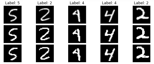
Figure 2: Original (the top row), binarized (the middle row), and perturbed with $\epsilon=1$ (the bottom row) sample MNIST images.

We present our results for adversarial robustness using the MNIST and IMDB datasets. To test adversarial robustness on an input $\mathcal{I}$, we experiment with three different $\epsilon$ perturbation values by varying $\epsilon\in\{1,3,5\}$. These values correspond to the maximum number of bit-flips applied on $\mathcal{I}$ when checking robustness using the SAT solver. The solver might take exponential time in the worst cases, so we impose a timeout of $300$ seconds on the solver for each test instance. This setup is the same for all experiments in this section. The range of $\epsilon$ and the timeout are chosen in this way to facilitate the comparison with BNNs [12] at the end of this section.

For multi-class problems, such as MNIST classification, the current state of the art of TsMs [7] creates one TsM $\mathcal{M}$ for each target class during the pre-processing phase. This means that the final trained model consists of a sorted team of TsMs where each member $\mathcal{M}_{i}$ will individually compute the sum (Eq. 1) that votes for class $i$. Given an interpretation $\mathcal{I}$ (in fact its vector representation) as input, the TsM team will output the class associated with the TsM that has the highest sum, as explained in Section 2.2.

As the MNIST dataset contains $10$ classes, we conduct the robustness experiment on each single TsM belonging to the trained TsM team. We test the adversarial robustness on $20$ randomly selected MNIST images per class, summing up to $200$ images. Table III presents the robustness results for the three MNIST models from Table I. Columns show the maximum number of bit-flips $\epsilon$, the number of instances solved by the SAT solver, the amount of them being $\epsilon$-robust, and the average time in seconds to solve these instances. “Solved” in this context means that the SAT solver either finds a valid perturbation leading to the change in the classification of the input image or that the model is $\epsilon$-robust on this image. Figure 2 illustrates examples of original images and perturbed images with $\epsilon=1$ (that is, with $1$-pixel flip) which led to a change in the classification.

TABLE III: Robustness on the MNIST dataset.

200 test instances
	model 1			model 2			model 3
$\epsilon$	solved	$\epsilon$-robust	time (sec)	solved	$\epsilon$-robust	time (sec)	solved	$\epsilon$-robust	time (sec)
1	200	171	0.92	200	184	2.81	200	184	13.85
3	162	45	26.11	57	29	105.85	7	5	258.36
5	124	0	70.61	12	0	268.54	0	0	$\geq$ 300

For $\epsilon=1$, all instances were solved withing the timeout of $300$ seconds and Models 2 and 3 (Table I), which are trained with more monomials, demonstrated greater resistance to input perturbations. However, increasing $\epsilon$ yields a more complex robustness encoding and solving more complex formulas, built from larger models such as Models 2 and 3, requires more time from the SAT solver. The solver was unable to complete any of the instances for $\epsilon=5$ for Model 3 within $300$ seconds (the timeout value).

Table IV presents the results of adversarial robustness for models trained on the IMDB dataset. The goal of this experiment is to study the effect of changing the specificity value of the TsMs for robustness verification. The experiment is run on $100$ test instances that were correctly classified by both models at the input without perturbation, that is, $\epsilon=0$. The models were trained to take a binary vector of $5000$ features as an input. Robustness test for $\epsilon=1$ creates $5000$ possible combinations of bit flips, that is, including or not including a word in the sentence (this is much more computationally challenging than the $28\times 28=784$ possible combinations of bit flips for $\epsilon=1$ in MNIST). For $\epsilon=5$, there are more than 120 billion possible combinations. Model 2 (and 3) with a low $s$ value, that stimulates negated reasoning, resulted in greater resistance to adversarial inputs, as expected [21]. Due to the fact that Model 2 contains fewer literals per monomial, it was able to solve more instances within 300 sec., with lower average computation time when compared to Model 1.

TABLE IV: Robustness on the IMDB dataset.

100 test instances
	model 1			model 2
$\epsilon$	solved	$\epsilon$-rob	time (s)	solved	$\epsilon$-rob	time (s)
1	98	36	42.73	100	56	10.92
3	54	0	233.59	83	17	69.72
5	49	0	217.95	83	8	64.50

IV-C Equivalence and Similarity

We run an equivalence test on the two models trained with the IMDB dataset using the same hyperparameter setup, that is, Model 2 and Model 3 from Table II. Both models achieved the same accuracy on the test set. This test aims to identify if two models trained on the same dataset and having the same accuracy would always give the same classification results for any input. The equivalence test, which verifies if their corresponding formulas are logically equivalent, showed them to not be fully equivalent in this strong sense. We then considered similarity, which is easier to achieve as it only requires that the classification matches in a number of instances, for a particular dataset. Table V presents the similarity experiment on a test set with $100$ instances. Columns show the number of instances solved by the SAT solver and the number of $\epsilon$-similar instances. “Solved’ in this context means that the SAT solver determines within 300 sec. whether two models return the same classification given an identical input (and perturbations of it quantified by $\epsilon$). The experiment is run with three different $\epsilon$ values. The results reported for $\epsilon=0$ show the similarity of two models in the input without perturbations. Models 2 and 3 are more consistent in their output predictions. They resulted in a single different classification for unperturbed input. Increasing the $\epsilon$ makes the SAT solver time out on several instances. Even then, Models 2 and 3 are $\epsilon$-similar on more instances for $\epsilon=1$.

TABLE V: Similarity check on the IMDB dataset.

100 test instances
	model 1 & model 2		model 2 & model 3
$\epsilon$	solved	$\epsilon$-similar	solved	$\epsilon$-similar
0	100	93	100	99
1	93	43	74	70
3	59	41	60	40

IV-D Comparison with BNNs

In this section, we compare TsMs and BNNs w.r.t. accuracy on the MNIST-c dataset and we discuss robustness in both cases on the MNIST-back-image dataset.

Accuracy Tests

Table VI shows the comparison of accuracy results on MNIST-c for the state-of-the-art TsM for MNIST (with $N=8000$, $T=6400$, and $s=5$.) and a BNN using the same hyperparamaters as in [9]. Both the TsM and the BNN are trained on the standard MNIST training data and tested on MNIST-c. Test images are sampled from MNIST-c as follows: with $p$ probability, a test image from the corrupted data is selected; one of the $15$ corruptions is selected with uniform probability, where $p=0$ means that the standard uncorrupted test data is used. In Table VI, we can see that the TsM achieves competitive accuracy results with different values of $p$, indicating good performance of TsMs in comparison with BNNs on the MNIST-c test data (note that when $p=0$ then we have the classical MNIST).

TABLE VI: Accuracy comparison on the MNIST-c dataset

MNIST-c	$p=0$	$p=0.25$	$p=0.5$	$p=0.75$
TsM	99.3	92.5	88.1	81.2
BNN	97.46	90.1	83.5	77.2

Robustness

We now consider the robustness results for BNN reported by Narodytska et al. in their work to verify the properties of BNNs [12], with the robustness results achieved by TsMs. Unfortunately, their code is not available to the community, making it impossible to rerun their code in the same conditions. We consider the results for $\epsilon$-robustness using the MNIST-back-image dataset, presented in the main text of in their paper. To visualize the results under similar conditions, we trained the TsM model using the MNIST-back-image dataset. Both the TsM and BNN models considered in this experiment are scaled down for robustness verification. The accuracy of the TsM (with $N=1000$, $T=25$, and $s=10$) after $400$ iterations was $81.56\%$ while the accuracy of the BNN model used by Narodytska et al. was $70\%$ [12]. We randomly selected $20$ images for each of the $10$ classes, which results in $200$ test instances.

TABLE VII: Robustness on the MNIST-back-image dataset.

200 test instances
	TsM			BNN
$\epsilon$	solved	$\epsilon$-rob	% $\epsilon$-rob	solved	$\epsilon$-rob	% $\epsilon$-rob
1	200	145	72.5%	191	138	72.25%
3	116	14	12.07%	107	20	18.69%
5	34	0	0%	104	3	2.88%

The experiment is run with three different perturbation values $\epsilon\in\{1,3,5\}$. It uses the same SAT solver as the authors of the BNN verification paper, i.e., Glucose, and the same timeout value of 300 seconds for each test instance. Table VII presents results for both models. The hardware used in both experiments is not the same. However, the percentages of $\epsilon$-robust instances in these two models are similar. This indicates that both models can have approximate robustness performance on MNIST-back-image perturbed inputs, however more tests are needed.

V Conclusion

We present an exact encoding of TsMs into propositional logic and we show how to verify properties such as adversarial robustness using a SAT solver, following an earlier approach for BNNs. We show the correctness of our encoding and present experimental results for adversarial robustness, equivalence, similarity. We then compare the accuracy between TsMs and BNNs, using the MNIST-c dataset (designed for testing accuracy with corrupted instances), and discuss robustness in both cases using the MNIST-back-image dataset. As future work, we plan to investigate optimizations of SAT solvers [9] for robustness verification.

VI Acknowledgements

Ozaki is supported by the NFR projects 316022 and 322480.

VII Learning with Tsetlin Machines

In this section we provide more details about TsMs [6] and a running example for sentiment classification.

VII-A Tsetlin Machines: Feedback Types

Figure 3: A Tsetlin Automaton (reward is represented on dashed arrows and penalty on simple arrows)

The name “Tsetlin Machine” originates from the Tsetlin Automaton (Figure 3), introduced by M. L. Tsetlin in 1961. TsMs use hardware-near bitwise operators, thereby minimizing the memory usage and computation cost. Furthermore, the whole learning process and recognition is based on bit manipulation. Before starting the TsM training, all the inputs need to be binarized. There exist several techniques for binarizing the dataset depending on the training data format and the objective of the model. For image classification tasks, it is recommended to binarize the training data using an adaptive Gaussian thresholding procedure [5]. Binarization will result in $1$ bit per pixel channel. Although TsMs have shown competitive accuracy results on simple grayscale image data sets such as MNIST or Fashion-MNIST, they still show quite poor accuracy for colored image datasets, for example, CIFAR-100, compared to other state-of-the-art models [5]. Binarizing natural language is less harmful because many text vectorization techniques already produce binary vectors, e.g., bag-of-words. As such, one loses less information than when binarizing image inputs.

The basic TsM for binary classification takes as input an $s$-dimensional vector $X=[x_{1},...,x_{s}]$ and produces a classification output $\hat{y}$. The output $\hat{y}$ is one of two possible classes, $\hat{y}=1$ or $\hat{y}=0$, corresponding to true and false. We associate each position in the input vector to a variable $x_{i}$, with $1\leq i\leq s$, and form a literal set

$$L=\{x_{1},...,x_{s},\neg{x_{1}},...,\neg{x_{s}}\}.$$

Trained TsMs are represented as formulas, using monomials, also called conjunctive clauses [6], $\mathcal{C}^{+}$ and $\mathcal{C}^{-}$, consisting of literals from the set $L$. The number of monomials is predefined by $n$, which is an input parameter to Algorithm 1. Half of the monomials are assigned positive polarity and the other half are assigned negative polarity. Thus, the size of $\mathcal{C}^{k}$, where $k\in\{+,-\}$, is $n/2$. The monomial outputs are combined into a classification decision, as explained in the main text (see Equation 1).

In simple words, the classification is based on majority voting where monomials with positive polarity are voting for true classification and monomials with negative polarity for false classification. This formula provides an interpretable explanation of the model, which is useful to check whether decisions are unfair, biased, or erroneous (see Example 1).

Each monomial $C^{k}(j)$ is composed from the set of literals $L$ whereby each of the literals is associated with its own TA. The automation decides whether to include or exclude a given literal from the literal set $L$ in the monomial $C^{k}(j)$. As illustrated in Figure 3, the decision to include or exclude a literal is based on the function $\mathcal{G}(\phi_{a})$, where $\phi_{a}$, $a\in\{1,2,...,2N\}$ is the current state of the TA.

$$\mathcal{G}(\phi_{a})=\begin{cases}exclude,&1\leq a\leq N\\ include,&N+1\leq a\leq 2N\end{cases}$$

$N$ is a hyperpartameter of the TsM model. The training procedure is given by Algorithm 1. The state transition of each Tsetlin Automaton governs learning. The reward transitions are indicated with solid lines in Figure 3, and the penalization transitions are indicated with dotted lines. Learning which literals to include in the monomials is based on reinforcement. Each monomial $C^{k}(j)$ is trained by receiving one of two types of feedback, depending on their polarity and desired output classification. Both feedbacks are stochastic. The value computed by the function $\sf clip$ in Algorithm 1 bounds the sum between the interval $[-T,T]$ and it is used to guide the random selection for the feedback type. Monomials can be given either a Type I Feedback that generalizes by producing frequent patterns or a Type II Feedback that specializes and strictly regulates the patterns [6].

Type I Feedback is given to the TA of monomials $C^{k}(j)$ when the output is equal to $k$ (that is, when they are correct). Table VIII contains the probabilities of receiving “Reward”, “Inaction”, or “Penalty” given the monomial polarity and literal value. Inaction feedback is a novel extension of the TA introduced by Granmo (2018). Inaction is simply leaving the TsM untouched. The variable $s$ is a hyperparameter fed to the learning algorithm that represents specificity. It controls how strongly the model prefers to include literals in the monomial. The greater $s$, the more literals are included.

Type II Feedback is given to the TA of monomial $C^{k}(j)$ when the output is not equal to $k$. Type II feedback actions are visualized in Table IX. Type I and Type II Feedbacks aim together at minimizing the output error.

Action	Monomial	1		0
	Literal	1	0	1	0
Incl.	P(Reward)	$\dfrac{s-1}{s}$	-	0	0
	P(Inaction)	$\dfrac{1}{s}$	-	$\dfrac{s-1}{s}$	$\dfrac{s-1}{s}$
	P(Penalty)	0	-	$\dfrac{1}{s}$	$\dfrac{1}{s}$
Excl.	P(Reward)	0	$\dfrac{1}{s}$	$\dfrac{1}{s}$	$\dfrac{1}{s}$
	P(Inaction)	$\dfrac{1}{s}$	$\dfrac{s-1}{s}$	$\dfrac{s-1}{s}$	$\dfrac{s-1}{s}$
	P(Penalty)	$\dfrac{s-1}{s}$	0	0	0

TABLE VIII: Type I Feedback

Action	Monomial	1		0
	Literal	1	0	1	0
Include	P(Reward)	0	-	0	0
	P(Inaction)	1.0	-	1.0	1.0
	P(Penalty)	0	-	0	0
Exclude	P(Reward)	0	0	0	0
	P(Inaction)	1.0	0	1.0	1.0
	P(Penalty)	0	1.0	0	0

TABLE IX: Type II Feedback

VII-B Tsetlin Machines: An Example Run

For a didactic example, consider a simple TsM with $2$ monomials in the (binary) sentiment classification task. Given an input vector $X$, the output can be classified as a positive sentiment or as a negative sentiment. During the pre-processing step, $5$ features

$$[\sf great,boring,bad,interesting,truly]$$

have been chosen to describe the sentiment. The features are binarized according to their presence in the sentence: if the word occurs in the sentence, the value is set to 1 and 0 otherwise. The binary vector is used to train the model.

The features form the literal set:

$$L=\{\sf great,boring,bad,interesting,truly,$$

$$\sf\neg{great},\neg{boring},\neg{bad},\neg{interesting},\neg{truly}\}$$

The hyperparameter $N$ is set to 5 which means that each automaton has $2N$ states. Figure 4 shows the initial memory state for both a positive monomial $C^{+}$ voting for positive classification, and anegative monomial $C^{-}$ voting for negative classification. The initial memory state is set to $5$ for all literals, which means that all are equally “Forgotten”.

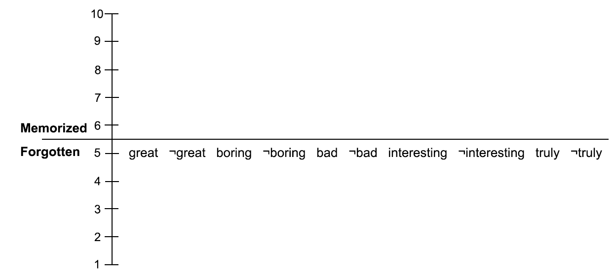
(a)

(b)

Figure 4: Initialization of the example run

Given the first input:

This movie was truly great and interesting $\rightarrow$ Positive

This sentence will produce an input vector $X_{1}=[1,0,0,1,1]$ and the label $y_{1}$ is positive. All literals are in the “Forgotten” state, so there are no literals to vote for any of the monomials. Empty monomials can be defined in different ways and, for simplicity of this example, we define both of them as $1$, that is, $C^{+}=1$ and $C^{-}=1$. We also skip the random selection of the monomials to receive feedback. The positive label $y_{1}$ for $X_{1}$ makes $C^{+}$ receive Type I Feedback and $C^{-}$ receive Type II Feedback. We have that $C^{+}$ votes for the true positive output class and it is boosted by Type I Feedback. In contrast, $C^{-}$ votes for false negative output and it is handled by Type II Feedback, which penalizes negative literals. Figure 5 illustrates literal evaluation for both monomials after receiving feedback. The black arrows indicates the high probability (1 or $\dfrac{s-1}{s}$), while gray arrows indicates low probability ($\dfrac{1}{s}$). The inaction feedback is omitted in the figure.

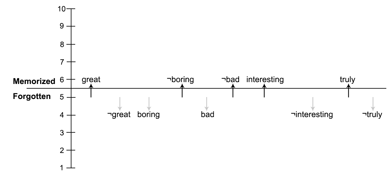
(a)

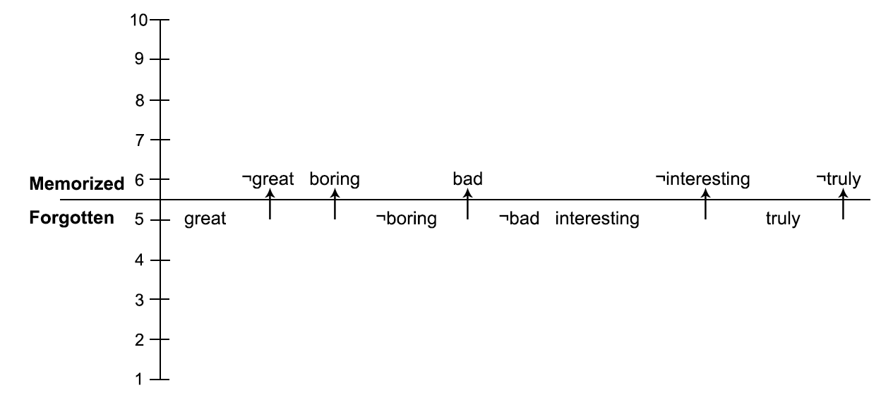
(b)

Figure 5: Memory update for “This movie was truly great and interesting $\rightarrow$ Positive”

Next, let the second input be:

Truly boring and bad movie $\rightarrow$ Negative

This sentence will produce an input vector $X_{2}=[0,1,1,0,1]$ and the label $y_{2}$ is negative. Figure 5 illustrates the “Memorized” literals voting for positive classification, which are

$$C^{+}=(\sf great\cdot\overline{boring}\cdot\overline{bad}\cdot interesting\cdot truly)$$

and “Memorized” literals voting for negative, which are

$$C^{-}=(\sf\overline{great}\cdot boring\cdot bad\cdot\overline{interesting}\cdot\overline{truly}).$$

Feeding the input $X_{2}$ to the monomials results in $C^{+}=0\cdot 0\cdot 0\cdot 0\cdot 1=0$ and $C^{-}=1\cdot 1\cdot 1\cdot 1\cdot 0=0$. The label $y_{2}$ is negative for $X_{2}$, therefore $C^{+}$ receives Type II Feedback and $C^{-}$ receives Type I Feedback. Type II Feedback penalizes only false positive outputs, so for $C^{+}$ the output is a true negative and all literals remain unchanged as seen in Figure 6. Type I Feedback is combating false negative output, that is, when $C^{-}$ is not trigged and the label $y_{2}$ is negative. The literals $\sf great,\neg boring,\neg bad,interesting,truly$ are in state $a_{i\in\{2,3,5,8,10\}}=6$, so there is an include action in Type I Feedback. Both positive and negative literals get penalized with equally low probability. The remaining literals are in state $a_{i\in\{1,4,6,7,9\}}=5$ meaning they perform exclude action which rewards all literals with low probability as well. Considering the probability, assume that only the literals marked with black color for the negative monomial in Figure 6 changed their state $a_{i\in\{1,4,10\}}$ by -1 (that is, $\sf great,\neg boring,\neg truly$,). The rest of the literals remained in the previous state of Figure 5.

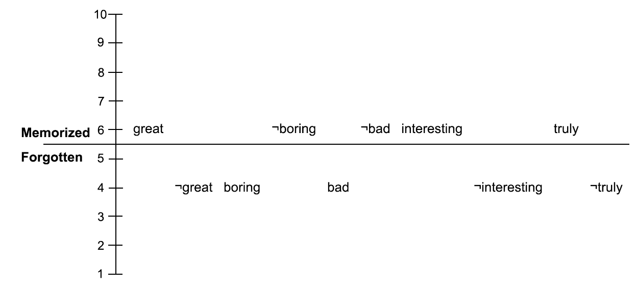
(a)

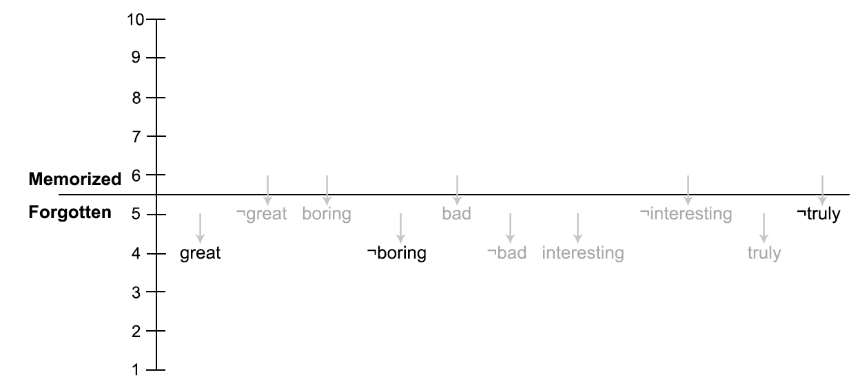
(b)

Figure 6: Memory update for “Truly boring and bad movie $\rightarrow$ Negative”

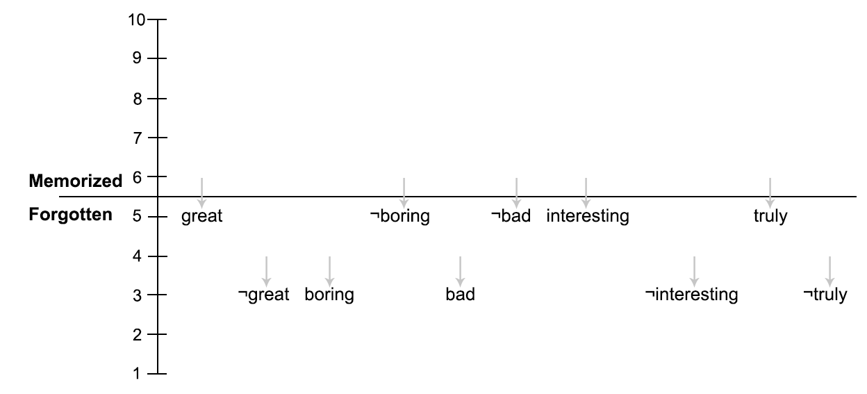
(a)

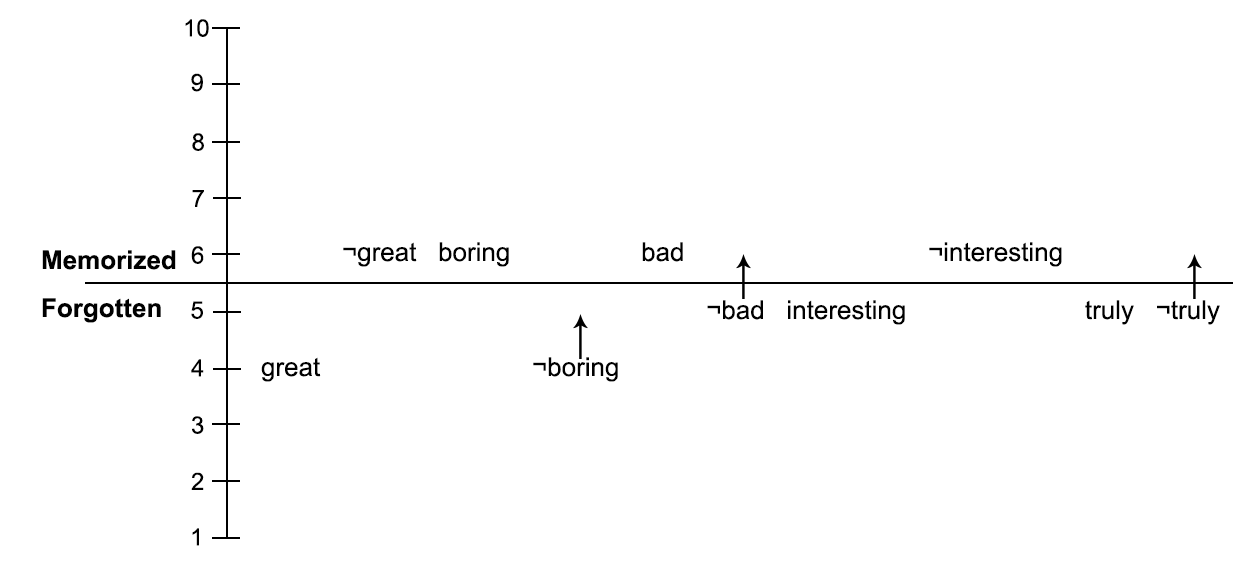
(b)

Figure 7: Memory update for “I thought this movie was going to be bad and boring but it was truly good $\rightarrow$ Positive”

Now, let the third input be:

I thought this movie was going to be bad and boring but it was truly good $\rightarrow$ Positive

This sentence will produce an input vector $X_{3}=[0,1,1,0,1]$ with the positive label $y_{3}$. The “Memorized” literals that vote for the negative monomial are now

$$C^{-}=(\sf\overline{great}\cdot boring\cdot bad\cdot\overline{interesting}).$$

The negative monomial will evaluate to $C^{-}=1\cdot 1\cdot 1\cdot 1=1$ being a false positive. Literals voting for $C^{+}$ are the same as previously, that is,

$$C^{+}=(\sf great\cdot\overline{boring}\cdot\overline{bad}\cdot interesting\cdot truly).$$

Given the input vector, $X_{3}$ the positive monomial is $C^{+}=0\cdot 0\cdot 0\cdot 0\cdot 1=0$, which implies that it will not vote for a positive classification. We then have a false negative. The positive label $y_{3}$ implies that Feedback Type I is provided to $C^{+}$, and Feedback Type II is given to $C^{-}$. Type I Feedback penalizes all of the literals being in the include state and rewards literals having exclude state, meaning all of the literals in the positive monomial decrements their states with a low probability of $1/s$. Negative monomials should seek to return 0 for the input $X_{3}$, but they do otherwise. All literals that are in the exclude zone, that is, states below or equal to 5, and whose value is 0 on the input ($\neg\sf boring,\neg bad,\neg truly$) are penalized with a probability of 1 by the Type II Feedback (Figure 7).

This finishes our illustrated presentation of how a TsM learns patterns from binary classified inputs. In the next section we provide proofs for the theorems in the main text.

VIII Proofs for Section III

See 2

Sketch.

Suppose there is an interpretation $\mathcal{J}$ that satisfies ${\sf NotRob}(\mathcal{M},\mathcal{I},\epsilon)$. In this case we want to show that $\mathcal{M}$ is not $\epsilon$-robust for $\mathcal{I}$. Since Eq. 6 is satisfied, we have $H_{n}(\mathcal{I},\mathcal{J})\leq\epsilon$, where $n$ is the dimension of the TsM with formula $\mathcal{M}$. By Theorem 1, the expression in Eq. 8 is satisfiable when the TsM formula classifies $\mathcal{J}$ differently from the classification of $\mathcal{I}$ (recall that we write $\mathcal{M}_{\vec{x}}$ instead of $\mathcal{M}$ just to make explicit the use of variables in $\vec{x}$). By Definition 1 this holds iff $\mathcal{M}$ is not $\epsilon$-robust for $\mathcal{I}$.

Conversely, if ${\sf NotRob}(\mathcal{M},\mathcal{I},\epsilon)$ is not satisfiable then there is no interpretation $\mathcal{J}$ which satisfies Eq. 6 and Eq. 7 (in other words, with hamming distance at most $\epsilon$ from $\mathcal{I}$) and is classified differently from $\mathcal{M}_{\vec{x}}(\mathcal{I})$. This means that $\mathcal{M}_{\vec{x}}$ is $\epsilon$-robust for $\mathcal{I}$. ∎

See 3

Proof.

By Theorem 2, each $c_{i}$ in Eq. 9 is set to true iff the TsM $\mathcal{M}$ is not $\epsilon$-robust for the given example $\mathcal{I}_{i}$. Therefore, Eq. 11 is satisfied iff the number of examples that do not pass the $\epsilon$-robustness condition is above the threshold $\lfloor\eta|S|\rfloor$. ∎

See 4

Proof.

By construction of $\varrho(\mathcal{M}_{i})$, for $1\leq i\leq 2$, the variables in $\vec{x}$ correspond to the input interpretation of the Tsetlin machine (TsM) $\mathcal{M}_{i}$. By Theorem 1 and since $\vec{x}$ is shared between the encodings of the two TsMs, $\mathcal{M}_{i}(\mathcal{I})=1$ iff $\varrho(\mathcal{M}_{i})_{[\vec{x}\rightarrow{\mathcal{I}}]}\wedge o^{i}$ is satisfiable. The formula $(\varrho(\mathcal{M}_{1})\wedge o^{1})\leftrightarrow(\varrho(\mathcal{M}_{2})\wedge o^{2})$ is falsified iff it is possible to find an $\mathcal{I}$ which is classified differently by the TsMs. ∎

See 5

Proof.

This theorem can be proven with arguments similar to those used for robustness and universal robustness. ∎

References

- [1] Kuruge Darshana Abeyrathna, Ole-Christoffer Granmo, and Morten Goodwin. Extending the tsetlin machine with integer-weighted clauses for increased interpretability. IEEE Access, 9:8233–8248, 2021.
- [2] Gilles Audemard and Laurent Simon. Predicting learnt clauses quality in modern SAT solvers. In Craig Boutilier, editor, IJCAI, pages 399–404, 2009.
- [3] Geir Thore Berge, Ole-Christoffer Granmo, Tor Oddbjørn Tveit, Morten Goodwin, Lei Jiao, and Bernt Viggo Matheussen. Using the tsetlin machine to learn human-interpretable rules for high-accuracy text categorization with medical applications. IEEE Access, 7:115134–115146, 2019.
- [4] Li Deng. The mnist database of handwritten digit images for machine learning research. IEEE Signal Processing Magazine, 29(6):141–142, 2012.
- [5] Ole-Christoffer Granmo, Sondre Glimsdal, Lei Jiao, Morten Goodwin, Christian W. Omlin, and Geir Thore Berge. The Convolutional Tsetlin Machine. arXiv preprint arXiv:1905.09688, 2019.
- [6] Ole-Christoffer Granmo. The Tsetlin Machine - A Game Theoretic Bandit Driven Approach to Optimal Pattern Recognition with Propositional Logic. arXiv:1804.01508, Apr 2018.
- [7] Ole-Christoffer Granmo. Pytsetlinmachine. https://github.com/cair/pyTsetlinMachine, 2020.
- [8] Kathrin Grosse, Nicolas Papernot, Praveen Manoharan, Michael Backes, and Patrick McDaniel. Adversarial examples for malware detection. In Simon N. Foley, Dieter Gollmann, and Einar Snekkenes, editors, Computer Security – ESORICS 2017, pages 62–79, Cham, 2017. Springer International Publishing.
- [9] Kai Jia and Martin Rinard. Efficient exact verification of binarized neural networks. In Hugo Larochelle, Marc’Aurelio Ranzato, Raia Hadsell, Maria-Florina Balcan, and Hsuan-Tien Lin, editors, NeurIPS, 2020.
- [10] Jie Lei, Tousif Rahman, Rishad Shafik, Adrian Wheeldon, Alex Yakovlev, Ole-Christoffer Granmo, Fahim Kawsar, and Akhil Mathur. Low-power audio keyword spotting using tsetlin machines. Journal of Low Power Electronics and Applications, 11, 2021.
- [11] Andrew L. Maas, Raymond E. Daly, Peter T. Pham, Dan Huang, Andrew Y. Ng, and Christopher Potts. Learning word vectors for sentiment analysis. In Dekang Lin, Yuji Matsumoto, and Rada Mihalcea, editors, Annual Meeting of the Association for Computational Linguistics, pages 142–150. The Association for Computer Linguistics, 2011.
- [12] Nina Narodytska, Shiva Prasad Kasiviswanathan, Leonid Ryzhyk, Mooly Sagiv, and Toby Walsh. Verifying properties of binarized deep neural networks. In AAAI, pages 6615–6624. AAAI Press, 2018.
- [13] Rupsa Saha, Ole-Christoffer Granmo, and Morten Goodwin. Using Tsetlin Machine to discover interpretable rules in natural language processing applications. Expert Systems, 2021.
- [14] Jivitesh Sharma, Rohan Yadav, Ole-Christoffer Granmo, and Lei Jiao. Drop Clause: Enhancing Performance, Interpretability and Robustness of the Tsetlin Machine. arXiv preprint arXiv:2105.14506, 2021.
- [15] Carsten Sinz. Towards an optimal cnf encoding of boolean cardinality constraints. In Peter van Beek, editor, Principles and Practice of Constraint Programming - CP 2005, pages 827–831, Berlin, Heidelberg, 2005. Springer Berlin Heidelberg.
- [16] Jiawei Su, Danilo Vasconcellos Vargas, and Kouichi Sakurai. One pixel attack for fooling deep neural networks. IEEE Trans. Evol. Comput., 23(5):828–841, 2019.
- [17] Michael Lvovitch Tsetlin. On behaviour of finite automata in random medium. Avtomat. i Telemekh, 22(10):1345–1354, 1961.
- [18] Adrian Wheeldon, Rishad Shafik, Tousif Rahman, Jie Lei, Alex Yakovlev, and Ole-Christoffer Granmo. Learning Automata based Energy-efficient AI Hardware Design for IoT. Philosophical Transactions of the Royal Society A, 2020.
- [19] Yi Xie, Zhuohang Li, Cong Shi, Jian Liu, Yingying Chen, and Bo Yuan. Real-time, robust and adaptive universal adversarial attacks against speaker recognition systems. J. Signal Process. Syst., 93(10):1187–1200, 2021.
- [20] Rohan Kumar Yadav, Lei Jiao, Ole-Christoffer Granmo, and Morten Goodwin. Human-Level Interpretable Learning for Aspect-Based Sentiment Analysis. In AAAI, 2021.
- [21] Rohan Kumar Yadav, Lei Jiao, Ole-Christoffer Granmo, and Morten Goodwin. Robust interpretable text classification against spurious correlations using and-rules with negation. In Luc De Raedt, editor, IJCAI, pages 4439–4446. ijcai.org, 2022.
- [22] Xuan Zhang, Lei Jiao, Ole-Christoffer Granmo, and Morten Goodwin. On the convergence of tsetlin machines for the identity- and not operators. IEEE Transactions on Pattern Analysis and Machine Intelligence, 44(10):6345–6359, 2022.
- [23] Yiyun Zhou, Meng Han, Liyuan Liu, Jing He, and Xi Gao. The adversarial attacks threats on computer vision: A survey. In 2019 IEEE 16th International Conference on Mobile Ad Hoc and Sensor Systems Workshops (MASSW), pages 25–30, 2019.