NeRF-DS: Neural Radiance Fields for Dynamic Specular Objects
Abstract
Dynamic Neural Radiance Field (NeRF) is a powerful algorithm capable of rendering photo-realistic novel view images from a monocular RGB video of a dynamic scene. Although it warps moving points across frames from the observation spaces to a common canonical space for rendering, dynamic NeRF does not model the change of the reflected color during the warping. As a result, this approach often fails drastically on challenging specular objects in motion. We address this limitation by reformulating the neural radiance field function to be conditioned on surface position and orientation in the observation space. This allows the specular surface at different poses to keep the different reflected colors when mapped to the common canonical space. Additionally, we add the mask of moving objects to guide the deformation field. As the specular surface changes color during motion, the mask mitigates the problem of failure to find temporal correspondences with only RGB supervision. We evaluate our model based on the novel view synthesis quality with a self-collected dataset of different moving specular objects in realistic environments. The experimental results demonstrate that our method significantly improves the reconstruction quality of moving specular objects from monocular RGB videos compared to the existing NeRF models. Our code and data are available at the project website 111https://github.com/JokerYan/NeRF-DS.
1 Introduction
Neural Radiance Fields (NeRF)[25] trained with multi-view images can synthesize novel views for 3D scenes with photo-realistic quality. NeRF predicts the volume density and view dependent color of the sampled spatial points in the scene with a multi-layer perceptron (MLP). Recent works such as Nerfies [33] and NSFF [22] extend NeRF to reconstruct dynamic scenes from monocular videos. They resolve the lack of multi-view image supervision in dynamic scenes using a deformation field, which warps different observation spaces to a common canonical space.
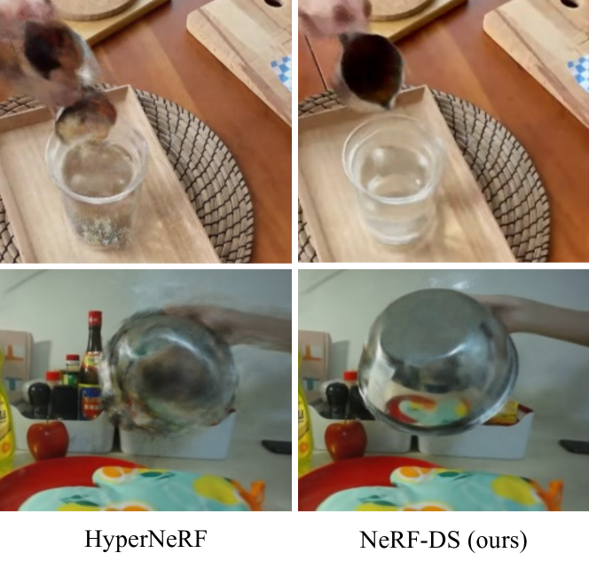
Despite showing promising results, we find that the existing dynamic NeRFs do not consider specular reflections during warping and often fail drastically on challenging dynamic specular objects as shown in Fig. 1. The quality of dynamic specular object reconstruction is important because specular (e.g. metallic, plastic) surfaces are common in our daily environment and furthermore it indicates how accurate a dynamic NeRF represents the radiance field under motion or deformation. Previous works such as Ref-NeRF [51] and NeRV [46] have only focused on improving the specular reconstruction in static scenes. The problem of reconstructing dynamic specular objects with NeRF remain largely unexplored.
We postulate that one of the reasons for dynamic models to fail on moving specular objects is because they do not consider the original surface information when rendering in a common canonical space. As suggested in rendering models such as Phong shading [35], the specular color depends on the relative position and orientation of the surface with respect to the reflected environment. Nonetheless, existing dynamic NeRFs often ignore the original position and orientation of the surface when warping a specular object to a common canonical space for rendering. As the result, a point on a specular object reflecting different colors at different positions and orientations can cause conflicts when warped to a common canonical space. Additionally, the key of existing dynamic models is to learn a deformation field for each frame such that correspondences can be established in a shared canonical space. However, the color of specular objects can vary significantly at different locations and orientations, which makes it hard to establish correspondences with the RGB supervision alone. These two limitations inevitably lead to the failure of existing dynamic models when applied to specular objects.
In this paper, we introduce NeRF-DS (Fig. 2) which models dynamic specular objects using a surface-aware dynamic NeRF and a mask guided deformation field to mitigate the two limitations mentioned above. 1) Our NeRF-DS still warps the points from the observation space to a common canonical space and predicts their volume density. In contrast to other dynamic NeRFs, the color of each point is additionally conditioned on the spatial coordinate and surface normal in the observation space before warping. Corresponding points from different frames can share the same geometry, but reflect different colors determined by their original surface position and orientation. 2) Our NeRF-DS reuses the moving object mask from the camera registration stage as an additional input to the deformation field. This mask is a more consistent guidance for specular surfaces in motion compared to the constantly changing color. The mask is also a strong cue to the deformation field on the moving and static regions. As shown in Fig. 1, our proposed NeRF-DS reconstructs and renders dynamic specular scenes with significantly higher quality.
We implement our NeRF-DS on top of the state-of-the-art HyperNeRF [34] for dyanmic scenes. Since there are very limited dynamic specular objects in the existing datasets, we collect another dynamic specular dataset for evaluation. Our dataset consists of a variety of moving/deforming specular objects in realistic environments. Experimental results on the dataset demonstrate that the NeRF-DS significantly improves the quality of novel view rendering on dynamic specular objects. The images rendered by our NeRF-DS avoid many serious artifacts compared to the existing NeRF models.
In summary, we have made the following contributions:
-
1.
A reparameterized dynamic NeRF that models dynamic specular surface with additional observation space coordinate and surface normal.
-
2.
A mask guided deformation field that improves deformation learned for dynamic specular objects.
-
3.
A dynamic specular scene dataset with training and testing monocular videos.

2 Related Work
Neural Scene Representation and Rendering.
The success of deep learning has led many works to explore suitable neural representations for 3D scene reconstruction and rendering. Explicit neural representations include point clouds[11, 55], meshes[1], and voxels[13, 49]. Recent works have also explored various implicit neural representations of 3D scenes. Level set based representations map spatial coordinates to a signed distance function (SDF)[32, 18, 56] or occupancy fields [24]. These methods usually focus on the geometry reconstruction of the scene and requires additional neural representation of the texture [30] to render the scene.
An alternative implicit neural representation is the neural radiance field (NeRF) [25, 2, 44]. NeRF directly represents the scene as a function that maps spatial coordinates and viewing angles to local point radiance. A differentiable volumetric rendering [25, 20] is performed to generate novel view images of the scene. NeRF can achieve photo-realistic novel view synthesis with only RGB supervision and known camera poses. Many extensions of NeRF are proposed, e.g. acceleration[52, 41], scene scale[48, 2], dynamic scenes[50, 34, 22] and specular surface rendering[51].
Dynamic Scene Reconstruction.
Dynamic scenes have objects moving in the foreground, objects undergoing deformation, or both. A simple reconstruction approach is to segment moving foreground and static background to reconstruct separately[54]. This method assumes the foreground is under rigid motion and cannot handle non-rigid deformation of the foreground object itself. A more general approach is to predict a canonical space and a temporal deformation field[27, 7, 23, 57, 29]. Many of these approaches require RGBD input [27, 57] or multiple camera inputs [23] to resolve the ambiguity in reconstructing moving objects.
Recent works [33, 34, 50, 36] based on the neural radiance field (NeRF) representation can jointly solve for canonical space and deformation field of dynamic scenes with only monocular RGB supervision. The canonical space in these works is usually a template NeRF as in static scenes, with the exception of HyperNeRF[34] which has additional hyper-coordinate input to model hyper canonical space. Another main difference among the existing dynamic NeRF models is the formulation of deformation field as a translation field [50, 36, 23] or a special euclidean () field [33, 34]. Since NeRF is a coordinate based representation of the scene, the existing dynamic NeRFs mostly focus on warping spatial coordinates with the deformation field. They do not consider the changes to the object surface explicitly during the warping.
Specular Surface Rendering.
Rendering photorealistic images of specular or reflective surfaces is one of the most difficult problems in computer graphics. It usually requires the global illumination to be considered, traditionally achieved by expensive algorithms such as radiosity[14, 9], ray tracing[16, 37] or photon mapping[17]. To speed up the rendering, a technique called precomputed radiance transfer (PRT)[45] is often used to precompute the lighting basis function in an environment map offline and rapidly sum them up during the online rendering phrase. For specular surfaces, the precomputation can be achieved by representing the reflection in spherical harmonics[3, 39, 40].
In neural representations like NeRF, most works focusing on specular surface rendering follow the idea of precomputation. The reflection environment map can be considered “precomputed” for each spatial point during the training. Some of the works based on the vanilla volumetric NeRF approximate the surface information needed for precomputation from volume density [51, 6, 47] or direct prediction [4, 60, 21]. Other works [58, 31, 56] based on the signed distance function approximate the surface information from the signed distance. NeRFReN [15] splits the radiance transmitted and reflected components with a mask to render large flat reflective surfaces. Ref-NeRF[51] proposes surface normal smoothing using MLP and directional encoding to further improve the performance. However, all the existing works in NeRF focusing on specular objects only consider static scenes instead of dynamic scenes.
3 Dynamic NeRF Preliminaries
NeRF[25] is a volumetric representation 333For simplicity in representations, we omit the output of in the equations below unless otherwise specified. of the scene. A multilayer-perceptron (MLP) is used to map the spatial position to a volume density and bottleneck output . Another MLP head takes in bottleneck and viewing direction (or outgoing radiance direction) to predict the color at the point:
| (1) |
To render an image of the scene, samples are taken on each pixel ray from camera center . The color of the pixel is the weighted sum of the colors at these sampled points, weighted by the product of accumulated transmittance based on step size and local volume density along the ray:
| (2a) | |||
| (2b) | |||
Dynamic NeRF [33, 34, 50, 36] reconstructs 3D dynamic scenes from monocular RGB camera footage. Since objects in a dynamic scene may be moving or deforming over time, only one frame is available for each moment of the scene. It is difficult to reconstruct the 3D structure of the scene without strict multi-view images. Consequently, most dynamic NeRFs transform the scene from an observation space at time to a common canonical space using a deformation field . Leveraging this common canonical space, images from different time and views can be used to reconstruct the scene with a static NeRF model :
| (3) |
In practice, the sampled observation space coordinate and the time embedding are fed into a deformation field prediction MLP to predict the canonical space coordinate . HyperNeRF[34] additionally predicts a hyper canonical coordinate from and using another MLP. The canonical coordinates and are supplied to the canonical NeRF MLP to predict the volume density . A color prediction head of the canonical NeRF MLP takes in viewing direction and outputs the color . The existing dynamic NeRFs are under-parameterized when rendering dynamic specular objects. Particularly, the color should also depend on the observation space surface normal and position . To this end, we propose to expand the model as . Refer to Sec. 4.1 for more details.
4 Our Method: NeRF-DS
Fig. 2 shows an illustration of our NeRF-DS which addresses the shortcomings of dynamic NeRFs for modeling the dynamic specular objects. Our NeRF-DS (on top of HyperNeRF[34]) includes a canonical NeRF conditioned on additional observation space position and orientation to predict the correct reflected color in the observation space (cf. Sec. 4.1). is obtained from ray samples and added with annealed positional encoding. is obtained from warping the surface normal predicted in the canonical space. To better learn the correspondence and deformation field of specular surfaces, the deformation field and hyper coordinate prediction are guided with a mask of the moving objects (cf. Sec. 4.2). is predicted by a mask prediction MLP and supervised by the 2D ground truth.
4.1 Surface-Aware Dynamic NeRF
In computer graphics, the rendering of specular surfaces is usually based on the rendering equation[38, 19]:
| (4) |
where is the outgoing radiance. The variables and represents the spatial coordinates, incident angle, outgoing angle, and surface normal, respectively. The first term represents the emission light when the target object is a light source. The second term is a reflection component which integrates the outgoing reflected radiance of all incoming radiance over the upper hemisphere based on the BRDF [28] and the environment map [10].
In NeRF models, the color of radiance is represented implicitly instead of integrated from all the reflected radiance explicitly. We can then simplify the reflection component to a function and the rendering equation becomes:
| (5) |
Under the assumption of no self-reflection, the reflected colors are all from the light source or objects in the static environment. The spatial coordinate , viewing direction and surface normal in Eq. 5 are expressed in the observation space.
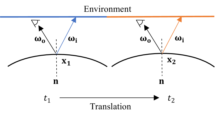
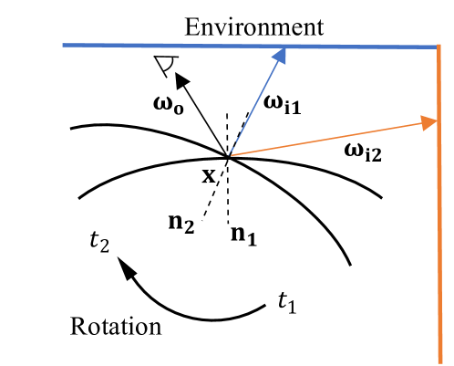
In static scenes, the surfaces of the object do not move and therefore there is no difference between the observation and canonical spaces. As a result, the surface normal can also be expressed as a function of denoted by , and hence the rendering equation simplifies to:
| (6) |
In dynamic NeRFs, moving objects are first mapped from the observation spaces to a common canonical space to render. The points at the same canonical space position and viewing direction are rendered the same color using NeRF MLP . However, as described in the rendering equation from Eq. 5, the color of the specular surface also depends on the observation space position and surface normal . Points with the same and , but different and might reflect different colors. The existing dynamic NeRF in the form of becomes an under-parameterized function in this case. Fig. 3 and 4 illustrate two simple scenarios where the existing dynamic NeRF formulation fails on specular surfaces.
We introduce a surface-aware dynamic NeRF following Eq. 5 to address the problem of under-parameterization in dynamic NeRFs. Surface information from the observation space is given to the canonical NeRF model to render the specular surface color. Specifically, we add the observation space coordinate and surface normal to the input of the NeRF color prediction branch (purple in Fig. 2) while keeping the volume density prediction branch unchanged. The modified NeRF function can then be expressed as:
| (7a) | ||||
| (7b) | ||||
To prevent the model from directly rendering in the observation space and thus ignoring the shared canonical space, we follow [33] to input the observation space coordinate with annealed position encoding :
| (8a) | ||||
| (8b) | ||||
The value of is initialized as 0 and slowly increased during training, so that is completely cut off from the model in the early training stage.
Unfortunately, the surface normal cannot be directly extracted from volumetric models such as NeRF. To circumvent this problem, we first estimate the canonical space surface normal with the negative gradient of volume density with respect to the canonical space coordinate [5, 46, 51]:
| (9) |
Nonetheless, the first order derivative of the volume density is noisy without direct supervision. We thus use the estimated to supervise a smoother predicted surface normal from the NeRF MLP and penalize any backward facing normal as in [51], i.e.:
| (10a) | |||
| (10b) | |||
We use 3D special Euclidean group () as our deformation field from the observation space to the canonical space. Finally, we can revert the canonical space surface normal back to observation space surface normal using:
| (11) |
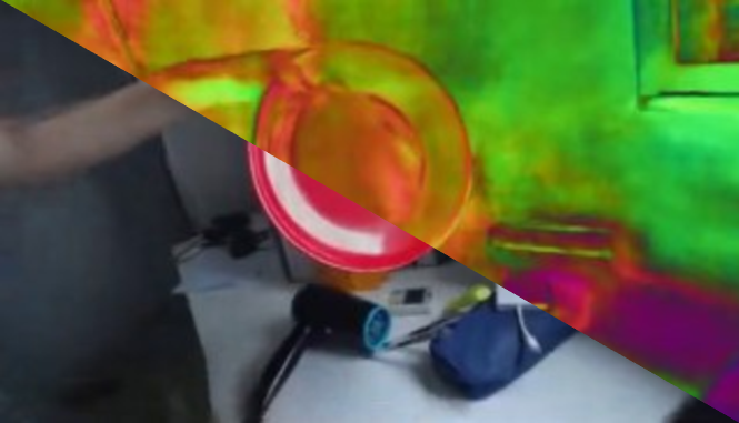
Predicting and then warping the surface normal in canonical space ensures the surface normal consistency over time. The surface normals and of two corresponding points at time and are related by . An example of final surface normal is illustrated in Fig. 5.
4.2 Mask Guided Deformation Field
Most non-specular objects do not change color drastically when moving. However, the color of specular objects can change significantly at different positions and orientations as shown in Eq. 5. The deformation of dynamic NeRFs is learned from RGB supervision only. Point correspondence can hardly be established if the color of the same point varies too much. As a result, the model often fails to learn the deformation field completely as shown in Fig. 6
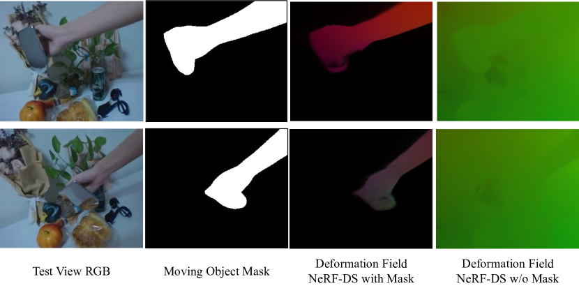
To mitigate this issue, we introduce a mask guided deformation field using a 2D mask of the moving objects. Unlike the drastically changing color of specular surfaces, this mask remains consistent during the object motion. It provides meaningful guidance toward the deformation field prediction for specular surfaces. Additionally, the mask gives a strong cue to the deformation prediction network on the deforming regions.
We thus add a mask prediction network that predicts the mask value at each 3D point in the observation space. The predicted mask is fed to the deformation field and hyper-coordinate prediction networks (blue in Fig. 2). The predicted 3D mask is supervised by the 2D mask in training views using volumetric rendering:
| (12) |
The mask prediction has more ambiguity than color prediction as the 2D mask is in binary values. We encourage the 3D mask to be predicted near the object surface by using sharper weights instead of . It is calculated by applying a Gaussian multiplier to weights for each sample . The Gaussian is centered at the maximum weights position and has a decreasing standard deviation during the training:
| (13) |
As shown in Fig. 6, the mask guided deformation field results in a more meaningful deformation field predicted.
We note that this mask is already required by most dynamic NeRF during the camera pose registration [33, 34, 22]. Moving foreground features must be masked out in structure-from-motion algorithms for correct registrations, thus we are not introducing additional input to the pipeline. Pose estimated without this mask can have significantly lower accuracy, especially when the moving part is large on the images. For example, camera poses estimated on our “basin” scene without masks are 31.7% deviated from the original poses after Procrustes alignment. HyperNeRF[34] trained on those poses performs 6.9% worse in PSNR and 82.7% worse in LPIPS.
5 Experiments
5.1 Dynamic Specular Dataset
Existing dynamic NeRF datasets, e.g. the scenes used in [33, 34, 22, 23] include almost no moving specular objects. We thus collect a new dynamic specular dataset for evaluation. Our dataset consists of 8 scenes in everyday environments with various types of moving or deforming specular objects. Each scene contains two videos captured by two forward-facing cameras rigidly mounted together, similar to the setup in [33]. The footage from one camera is used for training, and the other one is used for testing. This is different from the alternating training and testing cameras used in [33], which causes the “unrealistic teleporting camera” problem mentioned in [12]. Each video contains frames. The camera registration is performed using COLMAP [43, 42] after applying a mask generated from MiVOS [8]. This is the same mask used for mask prediction supervision in our mask guided deformation field module. See our supplementary for more details of the dataset.
5.2 Experimental Setups
We evaluate the performance of our model based on the novel view synthesis quality on the dynamic specular dataset mentioned above. The video frames of one camera are used for training, and the model generates the novel view images at the pose of the other camera. The generated images are compared with the ground truth test view images to calculate the following quantitative metrics: MS-SSIM[53], PSNR, LPIPS[59] as in previous works[34, 46, 22]. The average score across all the frames are reported.
We compare our model with the baseline models of HyperNeRF[34], Nerfies[33] and Ref-NeRF[51]. HyperNeRF achieves the state-of-the-art dynamic NeRF performance by introducing hyper-coordinates. Nerfies is a representative dynamic NeRF model with a standard canonical + deformation setup and outperforms many other models with similar designs. Ref-NeRF achieves the state-of-the-art reconstruction quality of static specular surfaces. These three baseline models well represent the SOTA performance of dynamic and specular scene reconstruction with NeRF.
Our implementation of NeRF-DS is based on HyperNeRF. The new mask prediction network is a 6-layer MLP with a width of 64. The final output of the mask prediction undergoes a ReLU activation. All baseline models and our models are trained following the respective official configuration for 250k iterations. All training and rendering are performed in resolution. More implementation details and experiment setup are in our supplementary.
5.3 Evaluation Results
In this section, we present the quantitative and qualitative results of our method compared to the baselines and the ablation models. Several videos of the rendered sequences are included in the supplementary.
| Mean | Bell | Plate | Sheet | ||||||||||||
| MS-SSIM | PSNR | LPIPS | MS-SSIM | PSNR | LPIPS | MS-SSIM | PSNR | LPIPS | MS-SSIM | PSNR | LPIPS | ||||
| Ref-NeRF [51] | .640 | 19.2 | .354 | .564 | 18.5 | .420 | .513 | 15.3 | .464 | .673 | 21.1 | .296 | |||
| Nerfies [33] | .689 | 19.7 | .381 | .696 | 19.9 | .389 | .489 | 15.4 | .599 | .834 | 23.6 | .183 | |||
| HyperNeRF [34] | .849 | 22.7 | .192 | .884 | 24.0 | .159 | .714 | 18.1 | .359 | .874 | 24.3 | .148 | |||
| NeRF-DS (Ours) | .890 | 23.4 | .135 | .872 | 23.3 | .134 | .867 | 20.8 | .164 | .918 | 25.7 | .115 | |||
| NeRF-DS w/o Surface | .881 | 23.3 | .142 | .867 | 23.2 | .141 | .861 | 20.8 | .171 | .905 | 25.2 | .124 | |||
| NeRF-DS w/o Mask | .881 | 23.3 | .153 | .887 | 23.9 | .138 | .855 | 20.5 | .196 | .887 | 24.7 | .141 | |||
| Sieve | Basin | Cup | Press | 2 Cups | |||||||||||
| MS-SSIM | PSNR | LPIPS | MS-SSIM | PSNR | LPIPS | MS-SSIM | PSNR | LPIPS | MS-SSIM | PSNR | LPIPS | MS-SSIM | PSNR | LPIPS | |
| Ref-NeRF [51] | .815 | 22.1 | .220 | .643 | 18.0 | .319 | .705 | 20.5 | .318 | .679 | 21.3 | .341 | .527 | 16.5 | .454 |
| Nerfies [33] | .823 | 21.8 | .232 | .635 | 18.1 | .368 | .750 | 20.7 | .293 | .720 | 21.3 | .377 | .563 | 17.1 | .605 |
| HyperNeRF [34] | .909 | 25.0 | .129 | .829 | 20.2 | .168 | .896 | 24.1 | .138 | .873 | 25.4 | .164 | .809 | 20.1 | .272 |
| NeRF-DS (Ours) | .935 | 26.1 | .108 | .868 | 20.3 | .127 | .916 | 24.5 | .118 | .911 | 26.4 | .123 | .836 | 20.4 | .193 |
| NeRF-DS w/o Surface | .935 | 26.2 | .107 | .868 | 20.3 | .128 | .918 | 24.6 | .117 | .886 | 25.8 | .140 | .810 | 20.3 | .211 |
| NeRF-DS w/o Mask | .928 | 26.0 | .112 | .835 | 20.1 | .149 | .912 | 24.4 | .122 | .894 | 26.1 | .142 | .849 | 20.9 | .220 |
Qualitative Results.
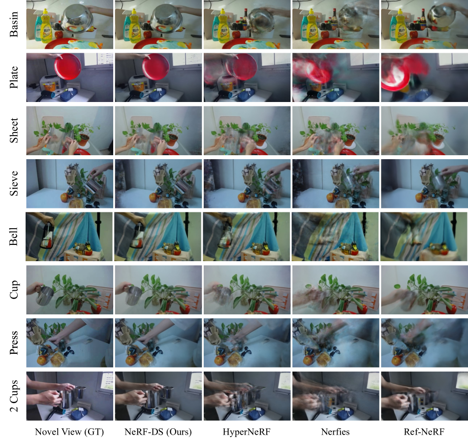
We present the qualitative results of novel view synthesis in Fig. 7. The HyperNeRF and Nerfies models tend to reconstruct dynamic specular objects with severe geometric artifacts. The rendered objects are blurry or torn apart along the moving trajectory. This can be attributed to two reasons: 1) The model struggles to capture the specular color without any observation space surface normal and location information. 2) The color of the specular object at the same point varies a lot, which makes it hard for the existing dynamic NeRF to learn a meaningful transformation field. This causes the sample points to warp to the wrong locations and resulting in the “torn-up” effect. Ref-NeRF also produces very blurry or torn-up results on dynamic specular objects. This is because Ref-NeRF assumes the scene to be static for all video frames. Since the object is actually moving, direct triangulation without warping would fail and thus leading to wrong prediction of the object geometry. Our NeRF-DS renders dynamic specular scenes with much fewer geometric artifacts. The reflected color on the specular surfaces is also relatively accurate. With the surface aware dynamic NeRF, the same canonical position is allowed to be mapped to different observation space positions reflecting different colors. The mask of moving objects guides the points in the observation space to learn the correct deformation mapping to the canonical space. As a result, the scene reconstructed by NeRF-DS is free from the “torn-up” effect present in other dynamic NeRFs. The reflected color is also more accurately controlled by the position and orientation of the surface.
Quantitative Results.
We report the quantitative results in Tab. 1. Note that LPIPS is taken to be a better measure of the construction quality compared to MS-SSIM and PSNR in previous works [33, 34]. During our qualitative evaluation, we also observe that MS-SSIM and PSNR are sometimes not affected significantly by blurry predictions. As shown in Tab. 1, our NeRF-DS outperforms all baseline models by a significant margin evaluated with LPIPS. NeRF-DS also has better MS-SSIM and PSNR scores in most scenes and the overall average.
Ablation Study.
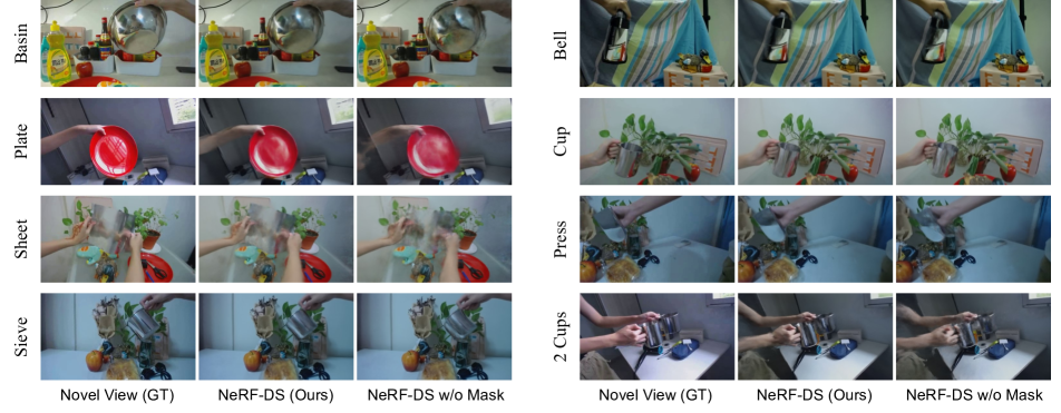
We evaluate the contributions of the two proposed components of our model: the surface-aware dynamic NeRF, and the mask guided deformation field by removing each of them at a time. The models without surface information and without masks are denoted as “NeRF-DS w/o Surface” and “NeRF-DS w/o Mask”, respectively. We report the quantitative comparisons in Tab. 1, and the qualitative comparisons in the supplementary. The results suggest that the performance drops when either component is removed, which verify the contribution of each component. Additionally, the superior performance of both ablation models compared to baselines further supports the effectiveness of our proposed methods.
6 Limitations
Although NeRF-DS significantly improves the reconstruction quality of dynamic specular objects, it relies on accurate surface normal predictions. Unfortunately, we have observed that the geometry of the surface predicted by NeRF can be misled by the reflected texture. The predicted surface normal takes the shape of the reflected textures instead of the surface geometry. This problem is more severe in dynamic specular scenes than in static specular scenes due to the lack of strict geometry constraints. We leave the exploration of surface priors or more constrained deformation models to our future work.
7 Conclusion
Our proposed NeRF-DS extends the prior dynamic NeRF to reconstruct and render dynamic specular scenes more accurately. We introduce surface-aware dynamic NeRF to address the under-parameterization problem of rendering specular surfaces in the canonical space. We further design a mask guided deformation field to learn better correspondence under constant color changes. Both components are essential to model reflected colors during the warping to the canonical space. Our NeRF-DS achieves a better novel view synthesis quality compared to the prior dynamic and reflective NeRFs on dynamic specular scenes.
Acknowledgement.
This research is supported by the National Research Foundation, Singapore under its AI Singapore Programme (AISG Award No: AISG2-RP-2021-024), and the Tier 2 grant MOE-T2EP20120-0011 from the Singapore Ministry of Education.
References
- [1] Timur Bagautdinov, Chenglei Wu, Jason Saragih, Pascal Fua, and Yaser Sheikh. Modeling facial geometry using compositional vaes. In Proceedings of the IEEE Conference on Computer Vision and Pattern Recognition, pages 3877–3886, 2018.
- [2] Jonathan T. Barron, Ben Mildenhall, Dor Verbin, Pratul P. Srinivasan, and Peter Hedman. Mip-nerf 360: Unbounded anti-aliased neural radiance fields. CVPR, 2022.
- [3] Ronen Basri and David W Jacobs. Lambertian reflectance and linear subspaces. IEEE transactions on pattern analysis and machine intelligence, 25(2):218–233, 2003.
- [4] Sai Bi, Zexiang Xu, Pratul Srinivasan, Ben Mildenhall, Kalyan Sunkavalli, Miloš Hašan, Yannick Hold-Geoffroy, David Kriegman, and Ravi Ramamoorthi. Neural reflectance fields for appearance acquisition. arXiv preprint arXiv:2008.03824, 2020.
- [5] Mark Boss, Raphael Braun, Varun Jampani, Jonathan T. Barron, Ce Liu, and Hendrik P.A. Lensch. Nerd: Neural reflectance decomposition from image collections. In 2021 IEEE/CVF International Conference on Computer Vision (ICCV), pages 12664–12674, 2021.
- [6] Mark Boss, Varun Jampani, Raphael Braun, Ce Liu, Jonathan Barron, and Hendrik Lensch. Neural-pil: Neural pre-integrated lighting for reflectance decomposition. Advances in Neural Information Processing Systems, 34:10691–10704, 2021.
- [7] Aljaz Bozic, Pablo Palafox, Michael Zollhöfer, Angela Dai, Justus Thies, and Matthias Nießner. Neural non-rigid tracking. Advances in Neural Information Processing Systems, 33:18727–18737, 2020.
- [8] Ho Kei Cheng, Yu-Wing Tai, and Chi-Keung Tang. Modular interactive video object segmentation: Interaction-to-mask, propagation and difference-aware fusion. In CVPR, 2021.
- [9] Michael F Cohen, John R Wallace, and Pat Hanrahan. Radiosity and realistic image synthesis. Morgan Kaufmann, 1993.
- [10] F. C. Crow. A more flexible image generation environment. SIGGRAPH Comput. Graph., 16(3):9–18, jul 1982.
- [11] Haoqiang Fan, Hao Su, and Leonidas J Guibas. A point set generation network for 3d object reconstruction from a single image. In Proceedings of the IEEE conference on computer vision and pattern recognition, pages 605–613, 2017.
- [12] Hang Gao, Ruilong Li, Shubham Tulsiani, Bryan Russell, and Angjoo Kanazawa. Monocular dynamic view synthesis: A reality check. In NeurIPS, 2022.
- [13] Rohit Girdhar, David F Fouhey, Mikel Rodriguez, and Abhinav Gupta. Learning a predictable and generative vector representation for objects. In European Conference on Computer Vision, pages 484–499. Springer, 2016.
- [14] Cindy M Goral, Kenneth E Torrance, Donald P Greenberg, and Bennett Battaile. Modeling the interaction of light between diffuse surfaces. ACM SIGGRAPH computer graphics, 18(3):213–222, 1984.
- [15] Yuan-Chen Guo, Di Kang, Linchao Bao, Yu He, and Song-Hai Zhang. Nerfren: Neural radiance fields with reflections. In Proceedings of the IEEE/CVF Conference on Computer Vision and Pattern Recognition, pages 18409–18418, 2022.
- [16] Vlastimil Havran and Jirí Bittner. LCTS: ray shooting using longest common traversal sequences. Comput. Graph. Forum, 19(3):59–70, 2000.
- [17] Henrik Wann Jensen. Realistic image synthesis using photon mapping, volume 364. Ak Peters Natick, 2001.
- [18] Chiyu Jiang, Avneesh Sud, Ameesh Makadia, Jingwei Huang, Matthias Nießner, Thomas Funkhouser, et al. Local implicit grid representations for 3d scenes. In Proceedings of the IEEE/CVF Conference on Computer Vision and Pattern Recognition, pages 6001–6010, 2020.
- [19] James T. Kajiya. The rendering equation. In Proceedings of the 13th Annual Conference on Computer Graphics and Interactive Techniques, SIGGRAPH ’86, page 143–150, New York, NY, USA, 1986. Association for Computing Machinery.
- [20] James T Kajiya and Brian P Von Herzen. Ray tracing volume densities. ACM SIGGRAPH computer graphics, 18(3):165–174, 1984.
- [21] Junxuan Li and Hongdong Li. Neural reflectance for shape recovery with shadow handling. In Proceedings of the IEEE/CVF Conference on Computer Vision and Pattern Recognition, pages 16221–16230, 2022.
- [22] Zhengqi Li, Simon Niklaus, Noah Snavely, and Oliver Wang. Neural scene flow fields for space-time view synthesis of dynamic scenes. In Proceedings of the IEEE/CVF Conference on Computer Vision and Pattern Recognition (CVPR), 2021.
- [23] Stephen Lombardi, Tomas Simon, Jason Saragih, Gabriel Schwartz, Andreas Lehrmann, and Yaser Sheikh. Neural volumes: Learning dynamic renderable volumes from images. arXiv preprint arXiv:1906.07751, 2019.
- [24] Lars Mescheder, Michael Oechsle, Michael Niemeyer, Sebastian Nowozin, and Andreas Geiger. Occupancy networks: Learning 3d reconstruction in function space. In Proceedings of the IEEE/CVF conference on computer vision and pattern recognition, pages 4460–4470, 2019.
- [25] Ben Mildenhall, Pratul P. Srinivasan, Matthew Tancik, Jonathan T. Barron, Ravi Ramamoorthi, and Ren Ng. Nerf: Representing scenes as neural radiance fields for view synthesis. In ECCV, 2020.
- [26] Ben Mildenhall, Dor Verbin, Pratul P. Srinivasan, Peter Hedman, Ricardo Martin-Brualla, and Jonathan T. Barron. MultiNeRF: A Code Release for Mip-NeRF 360, Ref-NeRF, and RawNeRF, 2022.
- [27] Richard A Newcombe, Dieter Fox, and Steven M Seitz. Dynamicfusion: Reconstruction and tracking of non-rigid scenes in real-time. In Proceedings of the IEEE conference on computer vision and pattern recognition, pages 343–352, 2015.
- [28] Fred E. Nicodemus, Joseph C. Richmond, Jack J. Hsia, Irving W. Ginsberg, and T. Limperis. Geometrical considerations and nomenclature for reflectance. 1977.
- [29] Michael Niemeyer, Lars Mescheder, Michael Oechsle, and Andreas Geiger. Occupancy flow: 4d reconstruction by learning particle dynamics. In Proceedings of the IEEE/CVF international conference on computer vision, pages 5379–5389, 2019.
- [30] Michael Niemeyer, Lars Mescheder, Michael Oechsle, and Andreas Geiger. Differentiable volumetric rendering: Learning implicit 3d representations without 3d supervision. In Proceedings of the IEEE/CVF Conference on Computer Vision and Pattern Recognition, pages 3504–3515, 2020.
- [31] Michael Oechsle, Songyou Peng, and Andreas Geiger. Unisurf: Unifying neural implicit surfaces and radiance fields for multi-view reconstruction. In Proceedings of the IEEE/CVF International Conference on Computer Vision, pages 5589–5599, 2021.
- [32] Jeong Joon Park, Peter Florence, Julian Straub, Richard Newcombe, and Steven Lovegrove. Deepsdf: Learning continuous signed distance functions for shape representation. In The IEEE Conference on Computer Vision and Pattern Recognition (CVPR), June 2019.
- [33] Keunhong Park, Utkarsh Sinha, Jonathan T. Barron, Sofien Bouaziz, Dan B Goldman, Steven M. Seitz, and Ricardo Martin-Brualla. Nerfies: Deformable neural radiance fields. ICCV, 2021.
- [34] Keunhong Park, Utkarsh Sinha, Peter Hedman, Jonathan T. Barron, Sofien Bouaziz, Dan B Goldman, Ricardo Martin-Brualla, and Steven M. Seitz. Hypernerf: A higher-dimensional representation for topologically varying neural radiance fields. ACM Trans. Graph., 40(6), dec 2021.
- [35] Bui Tuong Phong. Illumination for computer generated pictures. Commun. ACM, 18(6):311–317, jun 1975.
- [36] Albert Pumarola, Enric Corona, Gerard Pons-Moll, and Francesc Moreno-Noguer. D-NeRF: Neural Radiance Fields for Dynamic Scenes. In Proceedings of the IEEE/CVF Conference on Computer Vision and Pattern Recognition, 2020.
- [37] Timothy J. Purcell, Ian Buck, William R. Mark, and Pat Hanrahan. Ray tracing on programmable graphics hardware. In Proceedings of the 29th Annual Conference on Computer Graphics and Interactive Techniques, SIGGRAPH ’02, page 703–712, New York, NY, USA, 2002. Association for Computing Machinery.
- [38] Ravi Ramamoorthi. Precomputation-based rendering. Found. Trends. Comput. Graph. Vis., 3(4):281–369, apr 2009.
- [39] Ravi Ramamoorthi and Pat Hanrahan. An efficient representation for irradiance environment maps. In Proceedings of the 28th annual conference on Computer graphics and interactive techniques, pages 497–500, 2001.
- [40] Ravi Ramamoorthi and Pat Hanrahan. A signal-processing framework for inverse rendering. In Proceedings of the 28th annual conference on Computer graphics and interactive techniques, pages 117–128, 2001.
- [41] Christian Reiser, Songyou Peng, Yiyi Liao, and Andreas Geiger. Kilonerf: Speeding up neural radiance fields with thousands of tiny mlps. In Proceedings of the IEEE/CVF International Conference on Computer Vision, pages 14335–14345, 2021.
- [42] Johannes Lutz Schönberger and Jan-Michael Frahm. Structure-from-motion revisited. In Conference on Computer Vision and Pattern Recognition (CVPR), 2016.
- [43] Johannes Lutz Schönberger, Enliang Zheng, Marc Pollefeys, and Jan-Michael Frahm. Pixelwise view selection for unstructured multi-view stereo. In European Conference on Computer Vision (ECCV), 2016.
- [44] Vincent Sitzmann, Michael Zollhöfer, and Gordon Wetzstein. Scene representation networks: Continuous 3d-structure-aware neural scene representations. Advances in Neural Information Processing Systems, 32, 2019.
- [45] Peter-Pike Sloan, Jan Kautz, and John Snyder. Precomputed radiance transfer for real-time rendering in dynamic, low-frequency lighting environments. In Proceedings of the 29th Annual Conference on Computer Graphics and Interactive Techniques, SIGGRAPH ’02, page 527–536, New York, NY, USA, 2002. Association for Computing Machinery.
- [46] Pratul P. Srinivasan, Boyang Deng, Xiuming Zhang, Matthew Tancik, Ben Mildenhall, and Jonathan T. Barron. Nerv: Neural reflectance and visibility fields for relighting and view synthesis. In CVPR, 2021.
- [47] Pratul P Srinivasan, Boyang Deng, Xiuming Zhang, Matthew Tancik, Ben Mildenhall, and Jonathan T Barron. Nerv: Neural reflectance and visibility fields for relighting and view synthesis. In Proceedings of the IEEE/CVF Conference on Computer Vision and Pattern Recognition, pages 7495–7504, 2021.
- [48] Matthew Tancik, Vincent Casser, Xinchen Yan, Sabeek Pradhan, Ben Mildenhall, Pratul Srinivasan, Jonathan T. Barron, and Henrik Kretzschmar. Block-NeRF: Scalable large scene neural view synthesis. arXiv, 2022.
- [49] Maxim Tatarchenko, Alexey Dosovitskiy, and Thomas Brox. Octree generating networks: Efficient convolutional architectures for high-resolution 3d outputs. In Proceedings of the IEEE international conference on computer vision, pages 2088–2096, 2017.
- [50] Edgar Tretschk, Ayush Tewari, Vladislav Golyanik, Michael Zollhöfer, Christoph Lassner, and Christian Theobalt. Non-rigid neural radiance fields: Reconstruction and novel view synthesis of a dynamic scene from monocular video. In IEEE International Conference on Computer Vision (ICCV). IEEE, 2021.
- [51] Dor Verbin, Peter Hedman, Ben Mildenhall, Todd Zickler, Jonathan T. Barron, and Pratul P. Srinivasan. Ref-NeRF: Structured view-dependent appearance for neural radiance fields. CVPR, 2022.
- [52] Liao Wang, Jiakai Zhang, Xinhang Liu, Fuqiang Zhao, Yanshun Zhang, Yingliang Zhang, Minye Wu, Jingyi Yu, and Lan Xu. Fourier plenoctrees for dynamic radiance field rendering in real-time. In Proceedings of the IEEE/CVF Conference on Computer Vision and Pattern Recognition, pages 13524–13534, 2022.
- [53] Zhou Wang, Eero P Simoncelli, and Alan C Bovik. Multiscale structural similarity for image quality assessment. In The Thrity-Seventh Asilomar Conference on Signals, Systems & Computers, 2003, volume 2, pages 1398–1402. Ieee, 2003.
- [54] Yu-Shiang Wong, Changjian Li, Matthias Nießner, and Niloy J. Mitra. RigidFusion: RGB-D Scene Reconstruction with Rigidly-moving Objects. Computer Graphics Forum, 2021.
- [55] Yaoqing Yang, Chen Feng, Yiru Shen, and Dong Tian. Foldingnet: Point cloud auto-encoder via deep grid deformation. In Proceedings of the IEEE conference on computer vision and pattern recognition, pages 206–215, 2018.
- [56] Lior Yariv, Yoni Kasten, Dror Moran, Meirav Galun, Matan Atzmon, Basri Ronen, and Yaron Lipman. Multiview neural surface reconstruction by disentangling geometry and appearance. Advances in Neural Information Processing Systems, 33:2492–2502, 2020.
- [57] Tao Yu, Kaiwen Guo, Feng Xu, Yuan Dong, Zhaoqi Su, Jianhui Zhao, Jianguo Li, Qionghai Dai, and Yebin Liu. Bodyfusion: Real-time capture of human motion and surface geometry using a single depth camera. In Proceedings of the IEEE International Conference on Computer Vision, pages 910–919, 2017.
- [58] Jason Zhang, Gengshan Yang, Shubham Tulsiani, and Deva Ramanan. Ners: Neural reflectance surfaces for sparse-view 3d reconstruction in the wild. Advances in Neural Information Processing Systems, 34:29835–29847, 2021.
- [59] Richard Zhang, Phillip Isola, Alexei A Efros, Eli Shechtman, and Oliver Wang. The unreasonable effectiveness of deep features as a perceptual metric. In Proceedings of the IEEE conference on computer vision and pattern recognition, pages 586–595, 2018.
- [60] Xiuming Zhang, Pratul P Srinivasan, Boyang Deng, Paul Debevec, William T Freeman, and Jonathan T Barron. Nerfactor: Neural factorization of shape and reflectance under an unknown illumination. ACM Transactions on Graphics (TOG), 40(6):1–18, 2021.
Supplementary for
NeRF-DS: Neural Radiance Fields for Dynamic Specular Objects
1 Qualitative Result Videos
We include a few videos rendered by our model and the baseline models in the supplementary zip file as a better demonstration of the qualitative performance comparison.
2 Implementation Details
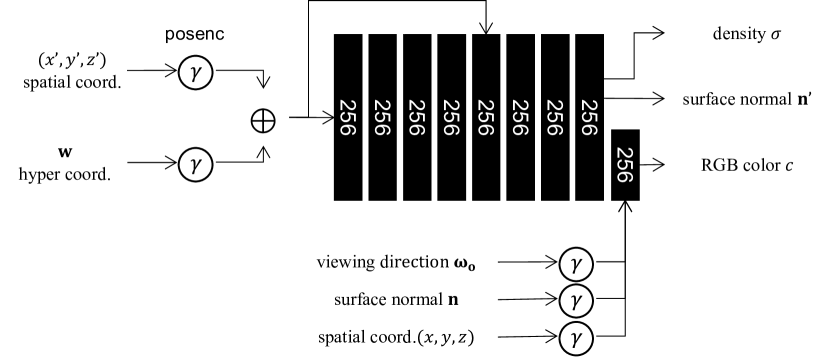
The details of the mask prediction module (Fig. 8), deformation prediction module (Fig. 9), hyper coordinate prediction module (Fig. 10) and canonical NeRF (Fig. 11) module are illustrated in the respective figure. Positional encoding is performed on spatial coordinates , , viewing direction and surface normal . Different encoding widths and annealing widths are used for different input as shown in Tab. 2. The Gaussian applied to the weights for mask volumetric rendering has an exponentially decreasing standard deviation from 1 to 0.1 during the first 30k iterations. Then it stays constant at 0.1 for the rest of the training.
2.1 Details of Ref-NeRF Experiments
2.2 Parameter and Training Time
The full model contains 1.45M parameters, compared to the 1.30M parameters of the baseline model. The experiment with 480x270 resolution videos takes 6 hours to train on 4 RTX A5000 GPUs, compared to the 5 hours training time of the baseline model.
| width | anneal | delay iter. | inc. iter. | inc. func. | |
|---|---|---|---|---|---|
| to mask | 4 | Yes | 0k | 50k | linear |
| to deformation | 4 | Yes | 0k | 50k | linear |
| to hyper coord. | 6 | No | N/A | N/A | N/A |
| to color branch | 4 | Yes | 50k | 50k | linear |
| to NeRF | 8 | No | N/A | N/A | N/A |
| to NeRF | 1 | No | N/A | N/A | N/A |
| to color branch | 4 | No | N/A | N/A | N/A |
| to color branch | 4 | Yes | 10k | 2k | linear |


3 Ablation Qualitative Results
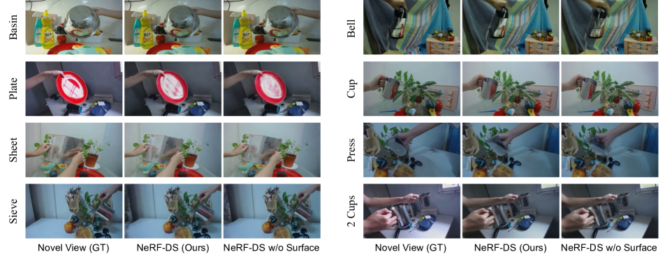
We present the qualitative comparison between the full and ablation versions of our models. The comparison between our NeRF-DS model and the ablation version without surface-aware dynamic NeRF is shown in Fig. 12. The comparison between our NeRF-DS model and the ablation version without mask guided deformation field is shown in Fig. 13.
4 Additional Experiment Results
We use delayed positional encoding for the spatial location and sharp volumetric weights for the mask rendering. In this section, we present additional ablation experiments to determine the best hyper-parameters for these two techniques.
We evaluate the performance of the NeRF-DS model on the “Sheet” scene in the dynamic specular dataset, under different annealing strategy of the positional encoding for the observation space spatial coordinate before it is fed to the NeRF color branch. Specifically, we evaluate the reconstruction performance with different schedules for the annealing coefficient of the th term in the position encoding as shown in:
| (14) |
We present the quantitative results in Tab. 3. Supported by the quantitative results, we choose to delay the use of in the NeRF color branch for the first 50k iterations, and slowly increase the bandwidth to a maximum of 4 during the next 50k iterations.
We also evaluate the performance of the NeRF-DS model on the “Sheet” scene in the dynamic specular dataset, with different sharp weights for mask rendering. Particularly, we evaluate the reconstruction performance with different schedules for decreasing standard deviation in the Gaussian filter applied to weight based on its ray distance :
| (15) |
We present the quantitative results in Tab. 4. Supported by the quantitative results, we choose to gradually decrease standard deviation for sharp mask weights from 1 to 0.1 during the first 30k iterations of the training.
Additionally, we evaluate the performance of the NeRF-DS model on the “Sheet” scene in the dynamic specular dataset, with surface normal calculated from different spaces. The surface normal in the observation space used in our main results are warped from the surface normal in the canonical space to ensure cross frame consistency, i.e. . We compare the results with the model using surface normal calculated in the canonical space and the surface normal directly calculated in observation space as shown in Tab. 5. The canonical space normal means . The observation space normal means the normal is supervised by the gradient of density with respect to the spatial coordinate in observation space:
| (16a) | |||
| (16b) | |||
Supported by the quantitative comparison, we choose to use the surface normal warped from the canonical space for the better consistency over time.
To demonstrate that our model has comparable performance to the baselines on non-specular dynamic scenes, we also present the experiment results of our model in the released scenes in the HyperNeRF dataset in Tab. 6. The results shown for Nerfies[33] and HyperNeRF[34] are taken from the original paper, while the performance of our model is reproduced on the same data. Please note that due to our limited hardware (compared to the 4 TPU used in the original paper), our model trained on this HyperNeRF[34] dataset is using 1/10 of the batch size and 10 times the number of iterations. The performance comparison in this way is slightly in our disadvantages, as our reproduced HyperNeRF[34] models under this setting perform worse than the reported models.
| Positional Encoding Annealing | MS-SSIM | PSNR | LPIPS |
|---|---|---|---|
| constant 4 | 0.911 | 25.4 | 0.118 |
| increase to 4 for 50k iter. | 0.915 | 25.7 | 0.119 |
| delay 10k, increase to 4 for 50k iter. | 0.914 | 25.6 | 0.121 |
| delay 50k, increase to 4 for 50k iter. | 0.918 | 25.7 | 0.115 |
| delay 100k, increase to 4 for 50k iter. | 0.917 | 25.7 | 0.117 |
| without x | 0.913 | 25.5 | 0.120 |
| Standard Deviation Schedule | MS-SSIM | PSNR | LPIPS |
|---|---|---|---|
| 1 to 0.01 for 30k iter. | 0.916 | 25.8 | 0.122 |
| 1 to 0.03 for 30k iter. | 0.905 | 25.3 | 0.125 |
| 1 to 0.1 for 30k iter. | 0.918 | 25.7 | 0.115 |
| 1 to 0.3 for 30k iter. | 0.917 | 25.7 | 0.120 |
| without sharping | 0.909 | 25.6 | 0.126 |
| Surface Normal | MS-SSIM | PSNR | LPIPS |
|---|---|---|---|
| Warped from canonical space | 0.918 | 25.7 | 0.115 |
| Canonical space normal | 0.913 | 25.5 | 0.119 |
| Observation space normal | 0.913 | 25.6 | 0.117 |
5 Additional Qualitative Analysis
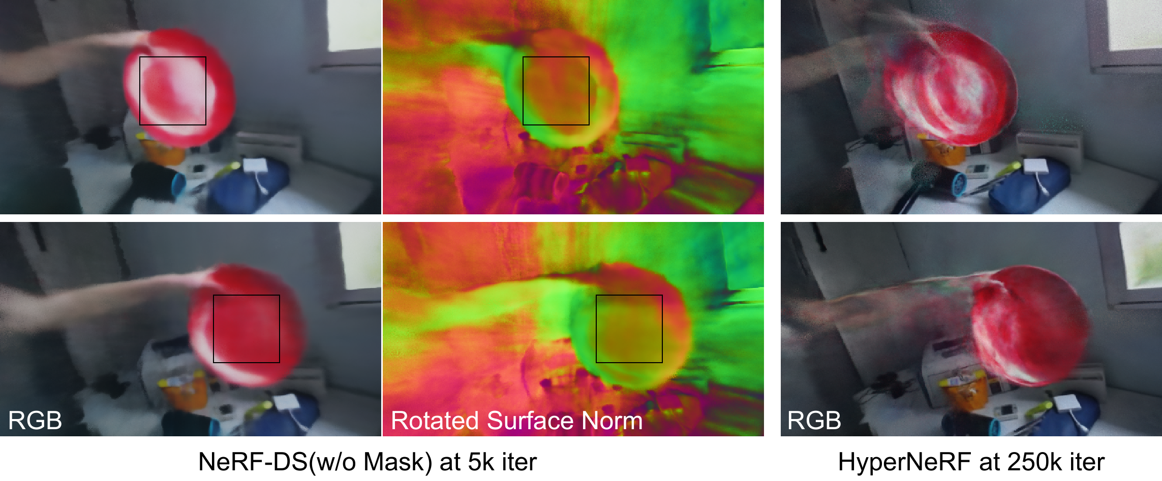
To further analyse the influence of the surface normal input on the rendering, we present a qualitative case study. Taking the early stage result of NeRF-DS (w/o mask) as an example (Fig. 15), the norms predicted for the middle part of the plate in two frames are different. With this input, our NeRF-DS model can render different reflected colors of the same surface. However, HyperNeRF fails to recognize the surfaces in the two frames to be the same and renders severe geometric artifacts. Additional masks can further suppress the geometric artifacts, but our ablation study suggests that the surface normal alone also contributes significantly to the performance (20.3% LPIPS improvement from baseline).
6 Dynamic Specular Dataset Details
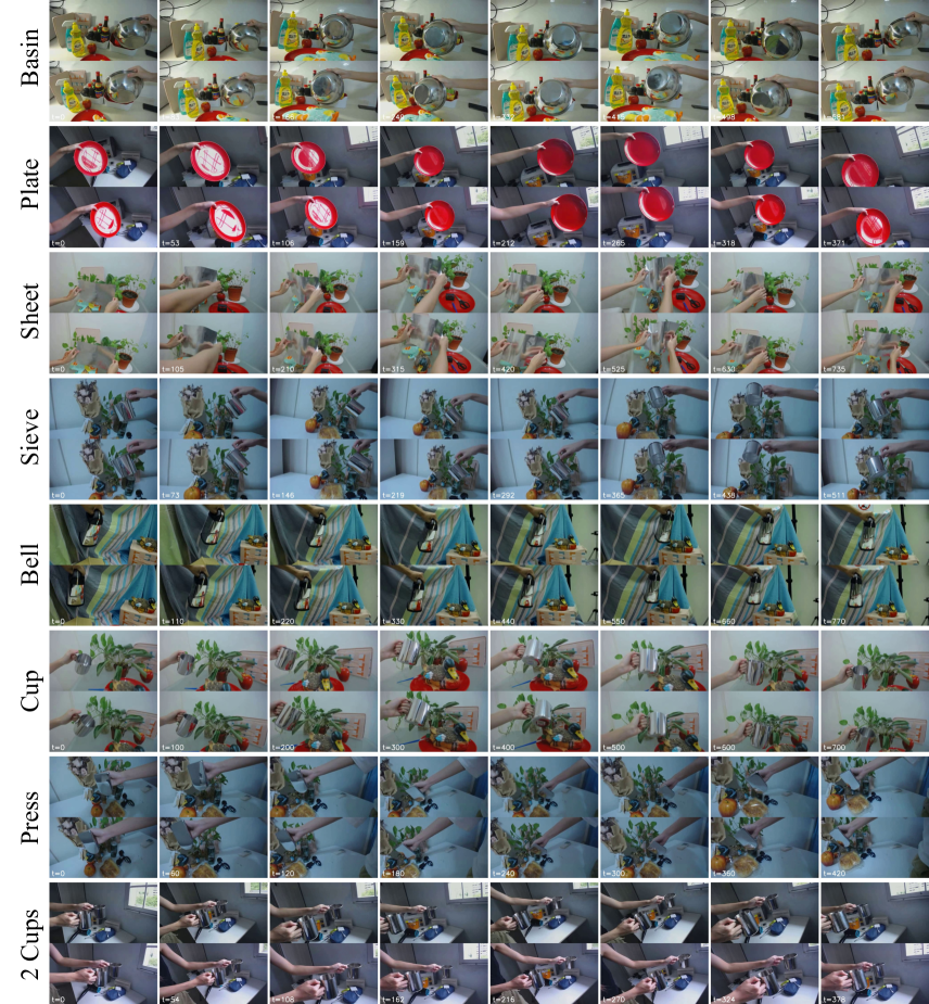
The dataset consists of 8 scenes of various dynamic specular objects in everyday environments. Two rigidly connected cameras are used to capture the scenes for 480x270 resolution. Different types of objects and surfaces are used as shown in Tab. 7. A snippet of the dataset is shown in Fig. 14. We appreciate the help of Liu Shiru and CVRP lab members for collecting this dataset.
| Scene Name | frames | Object Attribute |
|---|---|---|
| Basin | 668 | Curved+Flat, Metallic |
| Plate | 424 | Curved+Flat, Plastic, Colored |
| Sheet | 846 | Soft, Metallic, Non-Rigid Deformation |
| Sieve | 584 | Curved, Metallic, Porous Bottom |
| Bell | 881 | Slightly Curved, Metallic |
| Cup | 807 | Curved+Flat, Metallic |
| Press | 487 | Flat, Metallic |
| 2 Cups | 437 | Curved+Flat, Metallic, 2 Objects |