Equilibrium via multi-spin-flip Glauber dynamics in Ising Model

Abstract

Notwithstanding great strides that statistical mechanics has made in recent decades, an analytic solution of arguably the simplest model of relaxation dynamics, the Ising model in an applied external field remains elusive even in $1d$. Extant studies are based on numerics using single-spin-flip Glauber dynamics. There is no reason why this algorithm should lead to the global minimum energy state of the system. With this in mind, we explore multi-spin-flip parallel and sequential Glauber dynamics of Ising spins in $1d$ and also on a regular random graph of coordination number $z=3$. We view our study as a small initial step to test the generally implied hypothesis that the equilibrium is independent of the relaxational dynamics or if it carries some signature of it.

I Introduction

The grand task of statistical mechanics is to explain thermodynamics of systems with huge degrees of freedom. It is evidently a challenging task but made relatively easy in the domain of equilibrium statistical mechanics. A large class of isolated systems when left to themselves settle down in an equilibrium state which is characterized by small fluctuations with average value equal to zero on practical time scales. We can ignore such fluctuations and bypass their complicated dynamics. A simple overriding principle that a system in equilibrium is in a state of minimum free energy suffices to explain the observed behavior. Phase transition points and critical phenomena remained a challenge in equilibrium statistical mechanics for a long time because fluctuations at the critical point occur at all length scales. However, these too were tamed in recent decades by new techniques of the renormalization group theory  wilson .

In contrast, in the domain of nonequilibrium statistical mechanics, the fluctuations in the system do not average out to zero as the system approaches equilibrium very slowly or evolves in an inconveniently sporadic manner over observed time scales. In this difficult situation there is evidently no recourse available to us except to solve the equations of motion for impossibly large number of coupled degrees of freedom. Even to get a grip on the general principles of nonequilibrium statistical mechanics we have to be content only with a caricature of the system and its dynamics by some toy model. The Ising model and Glauber dynamics fit this bill  ising ; onsager ; glauber ; bertotti . In the following we describe our model and dynamics in detail. However it is not out of place here to mention the importance of hysteresis in our approach.

How do we know when a system has reached equilibrium or how far is it from it? This is not an easy question. In our approach, we rely on hysteresis for an answer. Hysteresis stands for history dependent dynamics of a system. The magnetization trajectory in increasing applied field is distinct from the one in decreasing field. The difference between the two is a measure of hysteresis in the system. The equilibrium state is by definition supposed to be independent of the initial state of the system. Thus hysteresis in the system serves as a signature of the distance from equilibrium in an evolving system. We may conclude that a system has reached equilibrium when it shows zero hysteresis. In our approach we consider two copies of a system magnetized to a saturation state in opposite directions and let the two copies evolve at the same value of the applied field for the same length of time. The difference between the two final states is taken as the distance of the system from equilibrium at that applied field.

II The Model

The Hamiltonian of the $1d$ Ising model is,

$$H=-J\sum_{i}s_{i}s_{i+1}-h\sum_{i}s_{i};s_{i}=\pm 1$$ (1)

Here $J$ is ferromagnetic ($J>0$) nearest neighbor interaction, $h$ is an applied field that is ramped up or down in suitable steps, $s_{i}$ is an Ising spin at site-$i$ on a chain of $N$ sites, $i=1,2,\ldots,N$. Periodic boundary conditions are assumed, i.e. $s_{i}\equiv s_{i+N}$. The magnetization per site is defined as $m=\sum_{i}s_{i}/N$.

The stochastic single-spin-flip Glauber dynamics associated with the Hamiltonian is prescribed as follows. The effective local field acting on spin $s_{i}(t)$ at site-$i$ at time $t$ is equal to $f_{i}(t)=J[s_{i-1}(t)+s_{i+1}(t)]+h$. The energy of the spin at site-$i$ is equal to $e_{i}(t)=-f_{i}(t)s_{i}(t)$ i.e. the energy is negative if $s_{i}(t)$ is aligned along the effective field $f_{i}(t)$, and positive otherwise. At each update moment the spin can flip with a probability $P_{i}(t)$ or stay unchanged with probability $1-P_{i}(t)$. The probability of flipping is larger if it lowers the energy. At temperature $T$, the probability of flipping is given by the following expression in terms of $K=J/(k_{B}T)$, $k_{B}$ being the Boltzmann constant,

$$P_{i}(s_{i}\rightarrow-s_{i}) =\frac{\exp(-Kf_{i}s_{i})}{\exp(-Kf_{i}s_{i})+\exp(Kf_{i}s_{i})}$$

$$=\frac{1}{1+\exp(2Ke_{i})}$$ (2)

Under parallel dynamics the entire set of spins $\{s_{i}(t)\}$ at time-$t$ is updated simultaneously producing $m(t+1)$ from $m(t)$ in one Monte Carlo time step or one MC cycle. Under sequential dynamics the spins are updated one at a time sequentially starting at site-$1$ and ending at site-$N$. For meaningful comparison with parallel dynamics we consider the update of the entire chain $i=1,\ldots,N$ in sequential dynamics as one MC cycle. We now present numerical results setting $J=1$ and $K_{B}=1$ for convenience, so that $K$ may be thought of as inverse temperature.

III Simulations

III.1 single-spin-flip dynamics

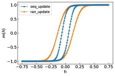
Figure 1: (Color online) Comparison for 1 spin-flip random vs sequential updating of spins: $L=2000$, $K=1.5$ and $t=50$ averaged over 200 configurations.

Fig.1 shows two hysteresis loops using single-spin-flip Glauber dynamics. A narrow loop obtained by sequential dynamics is symmetrically nested inside a larger loop for parallel dynamics. Both loops are for $K=1.5$ on a chain of length $N=2000$. At each applied field $h$, the system is allowed to evolve for $t=50$ MC cycles from an initial state with all spins parallel to each other. For the lower half of the loop, the initial state has all spins down and the field is ramped up in suitably small steps. On the upper half of the loop we start with all spins up and decrease the field till they are all turned down. The incremental steps for $h$ are chosen sufficiently small so that the data points for corresponding magnetization $m(h)$ appear as a smooth curve to the eye. Also contributing to the apparent smoothness of the curves is that each data point is an average over $200$ runs of the stochastic dynamics. We note that the hysteresis curves look remarkable similar to the observed hysteresis curves in the laboratory despite the model being just a toy model. Presumably this is the effect of the Boltzmann factor used in the Glauber dynamics. The Boltzmann factor determines thermal relaxation in any natural system. Why does the sequential dynamics yield a narrower loop? This is not too difficult to understand on reflection. In sequential dynamics each spin is relaxed in the shadow of its neighbor that has been relaxed earlier. So effectively the system has more opportunity to lower its energy in one MC cycle under sequential dynamics than under parallel dynamics. We are primarily interested in exploring algorithms that are more efficient for thermal relaxation. Therefore we confine ourselves to sequential dynamics in the following presentation. Of course the order in which $N$ spins are chosen for updating can be random rather than prefixed. We may choose the first spin randomly and then update all other spins sequentially along the chain. Or we may choose each of $N$ spins in one MC cycle randomly. We have explored this freedom to some extent but it does not seem to make a great deal of difference.

As may be expected, the hysteresis loops shown in Fig.1 become narrower when the system is relaxed for longer time. At $t=1000$ MC cycles the lower and upper halves of the loop appear to merge with each other on the scale of the figure. We interpret it to mean that the system has reached equilibrium. The equilibrium magnetization in an Ising chain in an external field $h$ can be determined analytically. Fig.2 shows that the equilibrium magnetization curve is indistinguishable from the collapsed hysteresis loops. This figure also shows the results of a simulation based on a two-spin-flip process which we discuss below. Suffice it to note here that the curve for the two-spin process at a lower value of $t=500$ is already indistinguishable from the single-spin-flip case at $t=1000$. Although the magnetization curves for one and two-spin flips in the long time limit merge with the equilibrium curve, it would be wrong to conclude that the corresponding thermodynamic states are identical. The equilibrium magnetization is based on a state which is obtained from the partition function. It takes into account all fluctuations in the system with corresponding Boltzmann weights. The long time limits obtained from dynamics necessarily comprise a restricted class of fluctuations. The correct conclusion to draw from our numerical results so far is that the average magnetization is not able to resolve the fine differences that must exist. We must search for other more revealing signatures of the differences.

III.2 two-spin-flip dynamics

There is no unique or standard algorithm to extend the single-spin-flip Glauber dynamics to a more general relaxation process. A rather obvious path is to incorporate simultaneous flips of a pair of neighboring spins or larger cluster of spins. Even here many variants are possible. We choose arguably the simplest of possible procedures which is as follows. Each MC cycle consists of two sub-cycles. The first sub-cycle implements single-spin-flips, and the next pairs of neighboring spins. The results are qualitatively similar to what might be expected from two successive MC cycles of single-spin-flips but are not identical to these. Fig.3 illustrates the result of a simulation for the same choice of parameters as in the earlier figures. As may be expected, two-flips move the system closer to equilibrium and consequently the loop narrows significantly.

Fig.1, Fig.2, and Fig.3 show hysteresis loops at a single value of inverse temperature $K=1.5$ but obtained by different procedures as described above. A remark about qualitative change in the shape of loop with varying $K$ is in order. At lower values of $K$ and moderate time periods $t$, the loop tends to elongate along the $x-$axis i.e. there is significant separation between lower and the upper halves over a larger range of applied field and remnant magnetization is relatively smallshukla1 . This is understandable because higher thermal energy weakens the ordering tendency of the applied field at moderate values of the applied field. At lower temperature and correspondingly higher $K$, the loop is elongated along the $y-$axis. In principle, hysteresis should vanish in the limit $t\rightarrow\infty$ irrespective of the value of $K$. However the relaxation becomes extremely slow at very large $K$ and it is difficult to observe the equilibrium limit of magnetization approaching a step function jump from $m=-1$ to $m=+1$ at $h=0$.

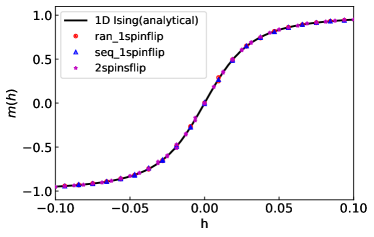
Figure 2: (Color online) Figure shows the convergence of the hysteresis loops of Fig1 to the equilibrium $1d$ Ising analytical values on increasing the relaxation time, $t=1000$. All data are averaged over 100 configurations. The curve corresponding to 2-spin-flip for $L=2000$, $K=1.5$ but $t=500$ is also shown for comparison.

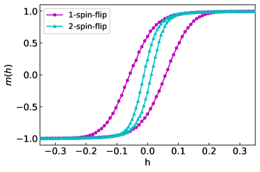
Figure 3: (Color online) Figure shows the smaller area of hysteresis loops on implementing 2-spin-flip dynamics compared to 1-spin-flip for the same set of parameters $L=2000$, $K=1.5$ and $t=50$. All data are averaged over 100 configurations.

III.3 hysteresis on regular random graphs

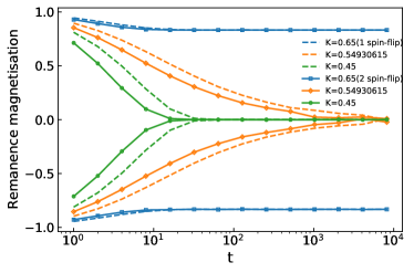
Figure 4: (Color online) The upper half of the figure shows how initial saturated magnetization in the up direction decays under various relaxation algorithms at zero applied external field and different temperatures. Similarly the lower half shows the increase of magnetization with time under relaxation on $z=3$ random graph for $L=10^{6}$ (averaged over 20 configurations). Other details as indicated in the figure.

A more promising route to explore the role of relaxation dynamics on the nature of equilibrium state which is eventually obtained is to go beyond a one dimensional Ising model. The one dimensional Ising model does not have a finite critical temperature. In other words, it does not order spontaneously below a finite temperature $T_{c}$. The simplest model which has a finite critical temperature $T_{c}$ whose value can be obtained analytically is the Ising model on a Bethe lattice with coordination number $z>2$. In this case the inverse critical temperature is given by the equation $\tanh K_{c}=1/(z-1)$ rozikov . For $z=3$, we get $K_{c}=0.5493$ approximately. The theory on the Bethe lattice can be checked quite effectively by simulations on regular random graphs. It is difficult to pin point the critical temperature exactly using dynamics but the presence of a watershed between high $K$ and low $K$ behaviour is easily spotted. Initial studies suggest the critical value $K_{c}$ obtained from 1-flip dynamics is in close vicinity of the analytical value $K_{c}=0.5493$ obtained from the equilibrium partition function. There may be some reason to expect $K_{c}$ obtained by dynamics to increase slightly as we go from one-flip to two-flip dynamics. This is because a combination of one and two spin flips may be able to explore deeper energy minima of the system. However we do not see a clear indication of this effect in our numerical work so far. Fig.4 presents the results of simulations at external applied field $h=0$, and three different values of $K=0.65,0.5493,$ and $0.45$. At each value of $K$, two sets of magnetization trajectories are shown in the same color, one starting with all spins down and the other with all spins up initially. At $K=K_{c}$ the magnetization approaches zero relatively slowly irrespective of the initial state. For $K<K_{c}$, it does the same but much faster as may be expected. For $K>K_{c}$, the system relaxes very slowly as may be expected and the magnetization remains close to the initial value over much of the observed times. We examined more closely the cases $K\leq K_{c}$ in the long time limit. Here the magnetization reaches a value nearly equal to zero within statistical fluctuations and the system may be said to be in a state of equilibrium. We examined if the fraction of neighboring spins parallel to reach other were in a higher proportion with two spin flips than with one spin flip dynamics. But we did not find any significant difference.

IV Future prospects

Our main concern in this article has been to investigate the equilibrium state of an isolated thermodynamic system. As Feynman  feynman put it, equilibrium is when fast things have happened and slow things have not. Thus equilibrium necessarily implies a separation between short and long time scales. Let us say $\Gamma$ is the characteristic time that separates these two. Then a system in equilibrium is thermalised with respect to fast relaxation processes with characterises time $\gamma<<\Gamma$ but not for slower processes. A great fortune of equilibrium statistical mechanics is that in the limit $\Gamma\rightarrow\infty$, properties of a system can be deduced from a knowledge of its partition function without knowing the dynamics. However a misfortune is that we can hardly ever evaluate a partition function exactly. Also experimental observations are obtained necessarily at a finite $\Gamma$. Thus we must resort to solving the dynamical equations which are not only too complex and coupled but also not known exactly for an extended complex system. We have to work with a set of model equations that hopefully might be tractable. Some hope in this direction is provided by a few models whose partition function or critical temperature has been evaluated exactly wannier . These are Ising models in one and two dimensions and on Bethe lattices of a general coordination number $z$. The Hamiltonians of these models are not true Hamiltonians in the sense of classical mechanics. The so called Hamiltonian does not generate Hamilton’s equations of motion. We have to put in a stochastic dynamics like Glauber’s dynamics by hand. Such dynamics can have different variants, e.g. single-flips or two-flips etc. There is no reason to expect if any of these variants would yield the same equilibrium state as the partition function. This is indeed a conundrum. On one hand we are accustomed to the belief that dynamics is unimportant in determining the properties of a system in thermal equilibrium. On the other hand it does look reasonable that the state of the system after a long time may retain some signature of the dynamics that brought it there. The preliminary work presented above is unfortunately not very conclusive in resolving this issue. One and two spin flips both appear to lead to equilibrium states that are hard to distinguish from each other. This may be an artifact of the Bethe lattice or may indicate a deeper truth of statistical mechanics. Nonetheless in our opinion it does raise an issue which has not received sufficient attention so far and needs to be explored further. We hope it is a small first step on a fruitful path.

V Acknowledgement

This write up has evolved from an earlier published work  shukla1 , and online presentations  shukla2 ; thongjaomayum in conferences over the last year or so.

References

- (1) See for example, K G Wilson and J Kogut, Phys. Rep. C 12, 77 (1974), and references therein.
- (2) E Ising, Z Phys 31, 253 (1925).
- (3) L Onsager, Phys Rev 65, 117 (1944).
- (4) R J Glauber, J Math Phys 4, 294 (1963).
- (5) See for example The Science of Hysteresis edited by G Bertotti and I Mayergoyz (Academic Press, Amsterdam, 2006).
- (6) U A Rozikov, Gibbs Measures on Cayley Trees, World Scientific (2013).
- (7) Statistical Mechanics: A set of lectures, by Richard P Feynman, Taylor and Francis, ABC ppbk, ISBN0-201-36076-2 (2018).
- (8) G H Wannier, Rev Mod Phys 17, 50 (1945); Phys Rev 79, 357 (1950).
- (9) Prabodh Shukla, Phys Rev E97, 062127 (2018).
- (10) Prabodh Shukla in Statistical Physics: Recent Advances and Future Directions (Online), ICTS, Bangalore (15 Feb, 2022).
- (11) Diana Thongjaomayum, XIII Biennial National Conference of Physics Academy of North East (2022), Manipur University, Imphal; International Conference on Advancement in Core and Frontier of Physics (2023), GLA University, Mathura.