Instant Domain Augmentation for LiDAR Semantic Segmentation
Supplementary Material

This material provides detailed information on handling dynamic objects, label consistency and propagation, detailed LiDAR configurations, and experiment settings. We also present per-class domain adaptation results, examples of the generated LiDAR scans, and more qualitative results from 3D semantic segmentation models trained with LiDomAug.

Appendix A Dynamic Objects

Algorithm 1 Dynamic object accumulation

1:Sequence of point clouds $\{\mathcal{P}_{n}\}_{n=1}^{N}$, 3D bounding boxes $\{\mathbf{b}_{n}^{k}\}_{n=1}^{N}$ of an object $k$, and its frame-to-frame transformation matrices $\{\mathbf{T}_{n}^{k}\}_{n=1}^{N}$

2:Accumulated points $\mathcal{P}^{k}$ of an object $k$

3:$\mathcal{P}^{k}\longleftarrow\{\ \}$

4:$\mathbf{T}\longleftarrow\mathbf{I}$

5:For $n=1:N$ do

6:     $\mathbf{T}\longleftarrow\mathbf{T}\circ(\mathbf{T}_{n}^{k})^{-1}$

7:     $\mathcal{P}^{k}\longleftarrow\{\mathcal{P}^{k}\cup\mathbf{T}(\mathcal{P}_{n}\cap\mathbf{b}_{n}^{k}))\}$

As described in the method section, object-wise motion causes an error, so-called flying points, in constructing the world model if we only use global ego-motion in the aggregation step. If the trajectories of each object over time are provided, the object-wise motion could be canceled out by applying the inverse of them, described in Algorithm 1.

As nuScene-lidarseg [nuscenes_lidarseg] dataset provides the information of object-wise motion in the form of 3D bounding box annotations, we apply the Algorithm 1 to build a better world model. On the other hand, the object-wise motion information is not available in SemanticKITTI [semantic_kitti]. In this case, we set a small temporal adjacency for dynamic objects to minimize the error while maximizing the density of the world model, then accumulate the 3D points on dynamic objects by applying global inverse ego-motion.

Algorithm 2 Label consistency check and propagation

1:Point clouds $\{\mathcal{P}_{n}\}_{n=1}^{N}$, its semantic label $\{\mathcal{L}_{n}\}_{n=1}^{N}$, ego-motion $\{\mathbf{T}_{n}\}_{n=1}^{N}$, and unlabeled point cloud $\mathcal{P}_{u}$

2:labels $\mathcal{L}$ for $\mathcal{P}_{u}$

3:$\mathcal{P}_{world}\longleftarrow\bigcup_{n=1}^{N}\mathbf{T}_{n}^{-1}(\mathcal{P}_{n})$

4:$\mathcal{L}_{world}\longleftarrow\bigcup_{n=1}^{N}\mathcal{L}_{n}$

5:$\{\mathbf{v}_{i}\}_{i=1}^{V}\longleftarrow$ Voxelization($\mathcal{P}_{world}$)

6:For $i=1:V$ do

7:     Make $\mathcal{J}=\{j\}$, s.t. $\mathbf{p}_{j}\in\mathbf{v}_{i}$ and $\mathbf{p}_{j}\in\mathcal{P}_{world}$

8:     Make $\mathcal{K}=\{k\}$, s.t. $\mathbf{p}_{k}\in\mathbf{v}_{i}$ and $\mathbf{p}_{k}\in\mathcal{P}_{u}$

9:     $l^{*}_{i}$ = MostFrequent$(\{l_{j}|j\in\mathcal{J}\})$, s.t. $l\in\mathcal{L}_{world}$

10:     $\mathcal{L}(\mathcal{J})\leftarrow l^{*}_{i}$ $\triangleright$ Label consistency

11:     $\mathcal{L}(\mathcal{K})\leftarrow l^{*}_{i}$ $\triangleright$ Label propagation

Appendix B Label consistency check and propagation

Whereas SemanticKITTI [semantic_kitti] provides 3D semantic labels for every frame, nuScene-lidarseg [nuscenes_lidarseg] dataset provides labels only for key-frames sampled at 2Hz. Also, it is difficult for human labelers to label 3D points accurately when the semantics change (e.g., the boundary of the object) or the 3D points are too sparse, so labeling errors occur. As described in the method section, we prepare an examination step for label consistency check and propagation. The 3D points in a world model are divided by a small voxel grid ($0.1m\times 0.1m\times 0.1m$), and the representative labels for each voxel are determined by majority voting. Based on the representative labels, we can correct the semantic labels of 3D points or assign a new label to the unlabeled 3D points. The detailed description of this procedure is shown in Algorithm 2. During this procedure, 6.4 points (nuScenes-lidarseg [nuscenes_lidarseg]) or 8.8 points (SemanticKITTI [semantic_kitti]) are assigned to a single voxel in average.

Model	Velodyne HDL-64E	Velodyne HDL-32E	Velodyne VLP-16	Ouster OS-1 64	Ouster OS-1 128
Channels ($H$)	64	32	16	64	128
Range ($r$)	120 m	100 m	100 m	120 m	120 m
Field of View ($f_{up},f_{down}$)	+2.0°to -24.9°	+10.67°to 30.67°	+15.0°to -15.0°	+22.5°to -22.5°	+22.5°to -22.5°
Horizontal angular resolution ($W$)	2048	2048	2048	1024	1024
Clock-wise rotation rate ($\omega_{0}$)	20Hz	20Hz	20Hz	20Hz	20Hz

Table A1: Detailed configurations of various LiDARs used in our experiments

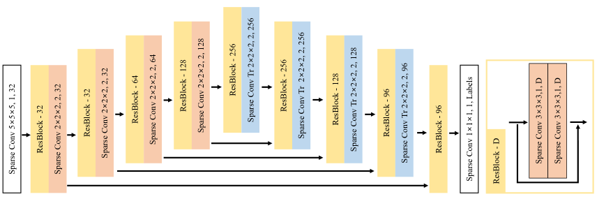
Figure A1: Architecture of MinkowskiNet42(Res16UNet34)[Minkowski]. ‘Sparse Conv Tr’ means transposed sparse convolution.

Appendix C Details of LiDAR Configuration

As mentioned in the experimental section (Table 3), we consider five popular LiDARs from different vendors such as Velodyne[velodyne2007] and Ouster[ouster2018]. Table B shows the specifications of the considered LiDARs.

Appendix D Experiment Settings

Architecture.

We use MinkNet42 [Minkowski], and a variant of MinkNet from C&L [complete_and_label_cvpr21] and SPVCNN [SPVNAS_ECCV20] as our baselines. We implement the sparse-convolution-based SPVCNN backbone using MinkowskiEngine [Minkowski] for a NAS-based backbone experiment. And the MinkNet42 consists of five planes of the encoder and four planes of the decoder. Each res-blocks is set to [32, 64, 128, 256, 256, 128, 96, 96] dimensions with two convolution layers each. Figure A1 shows the MinkNet42 architecture we use throughout the experiments. For C&L backbone, we follow the details in C&L paper [complete_and_label_cvpr21] to implement the U-Net style custom MinkNet, which has [24, 32, 48, 64, 80, 96, 112] dimensions for the encoder blocks and [96, 80, 64, 48, 32, 16] dimensions for the decoder blocks. Please refer to the original paper [complete_and_label_cvpr21] for more details. We use voxel size as $d=5cm$ for all three backbones.

Training.

We use SGD optimizer with the momentum of $0.9$ and weight decay of $10^{-4}$. The initial learning rate is set to $10^{-1}$, decayed by $0.1$ at [3, 8, 15] epochs. We use a batch size of four and use the cross-entropy loss. The training and evaluation are done with a single NVIDIA GeForce RTX 3090 GPU.

Appendix E Additional Domain Adaptation Scenarios

		Unit: mIoU (Rel.%)
Backbone (# of params)	Methods	Source $\rightarrow$ Target
		$K\rightarrow P$		$N\rightarrow P$
MinkNet42 [Minkowski] (37.8M)	Baseline	9.5		11.3
	Baseline + LiDomAug	11.5	($\uparrow$ 21.1)	28.1	($\uparrow$ 148.6)

Table A2: Training with SemanticKITTI [kitti] and testing with Pandaset [pandaset] (K$\rightarrow$P) and vice versa (N$\rightarrow$P) with MinkNet42 [Minkowski]

We conduct an additional experiment on Pandaset [pandaset], which consists of one forward-facing solid-state LiDAR and one spinning Hesai LiDAR, to investigate whether LiDomAug is effective beyond a single cylindrical LiDAR setup. We train models on SemanticKITTI or nuScenes and evaluate them on Pandaset. The results, as shown in Table. E, reveal that our method is effective in both $K\rightarrow P$ and $N\rightarrow P$ scenarios, indicating the potential advantages of our method in complex LiDAR setups.

Backbone	Methods	mIoU	mAcc	car	bicycle	motorcycle	truck	other vehicle	pedestrian	drivable surface	sidewalk	terrain	vegetation	Avg. rank
MinkNet42	Baseline	37.8	48.1	50.7	5.65	5.96	21.7	24.8	29.2	89.1	42.0	23.1	85.8	3.5
	CutMix [Cutmix]	37.1	46.4	75.5	0.05	14.0	26.6	22.6	3.92	86.6	36.5	19.7	85.6	4.7
	Copy-Paste [Copy-Paste]	38.5	48.8	77.9	3.11	11.1	21.7	31.2	7.81	88.0	38.8	19.6	86.2	3.6
	Mix3D [Mix3d]	43.1	52.7	72.1	0.00	34.8	11.7	26.4	28.5	83.3	41.0	46.4	86.5	3.7
	Polarmix [Polarmix]	45.8	54.4	74.1	1.68	41.9	26.9	23.8	30.5	85.1	42.7	45.3	86.2	2.7
	Baseline+LiDomAug	45.9	55.0	79.2	5.78	28.0	49.3	32.1	13.8	88.0	42.0	35.4	85.1	2.4

Table A3: Per-class accuracy from various data augmentation methods. All the models are trained on SemanticKITTI, and tested on nuScene-lidarseg (K$\rightarrow$N).

Backbone	Methods	mIoU	mAcc	car	bicycle	motorcycle	truck	other vehicle	pedestrian	drivable surface	sidewalk	terrain	vegetation	Avg. rank
MinkNet42	Baseline	36.1	46.9	78.5	0.00	8.17	3.37	11.1	34.5	66.3	35.8	39.4	84.2	4.5
	CutMix [Cutmix]	37.6	51.4	81.2	0.00	5.28	9.09	17.4	11.8	73.6	45.5	46.8	85.7	3.9
	Copy-Paste [Copy-Paste]	41.1	56.6	85.7	0.00	8.17	12.8	6.46	28.6	80.8	47.4	53.8	87.2	2.8
	Mix3D [Mix3d]	44.7	63.9	93.1	10.4	31.3	17.0	14.1	34.2	71.8	40.7	44.6	89.5	2.8
	Polarmix [Polarmix]	39.1	61.2	75.9	19.4	19.7	9.60	3.03	18.3	75.0	43.1	48.9	77.8	4.0
	Baseline+LiDomAug	48.3	69.0	92.6	31.6	42.5	21.6	6.43	34.4	70.0	47.1	59.4	77.5	2.6

Table A4: Per-class accuracy from various data augmentation methods. All the models are trained on nuScene-lidarseg, and tested on SemanticKITTI (N$\rightarrow$K).

Appendix F Per-class Domain Adaptation Results

In Table A3 (K$\rightarrow$N) and Table A4 (N$\rightarrow$K), we present per-class IoU numbers from our experiments, and Baseline + LiDomAug achieves the best performances in mIoU, mAcc, and avg. rank metrics. Particularly, as shown in Table A4 (N$\rightarrow$K), our Baseline + LiDomAug setting, in which the label propagation and dynamic object handling are applied, significantly improves the performance of moving object classes (bicycle: $0.00\rightarrow 31.6$, motorcycle: $8.17\rightarrow 42.5$, truck: $3.37\rightarrow 21.6$). Note that our final model, Baseline+LiDomAug, achieves the best performance in average rank across classes, implying that LiDomAug helps the model generalize over multiple classes beyond sensor-shift.

Appendix G More Qualitative Results

We included a video file, LiDomAug.mp4, to showcase (1) augmented frames using LiDomAug, (2) dynamic object accumulation, and (3) label consistency check and propagation. We also present the qualitative results of (4) the evaluation of generated LiDAR frames and (5) the evaluation of two different datasets. Figure A2 and A3 represent the qualitative examples from LiDomAug in SemanticKITTI. Our data generation can imitate the LiDAR geometric patterns with various configurations. Figure A4, A5, A6 shows the qualitative comparison between the model trained with and without LiDomAug, and show significant improvement.

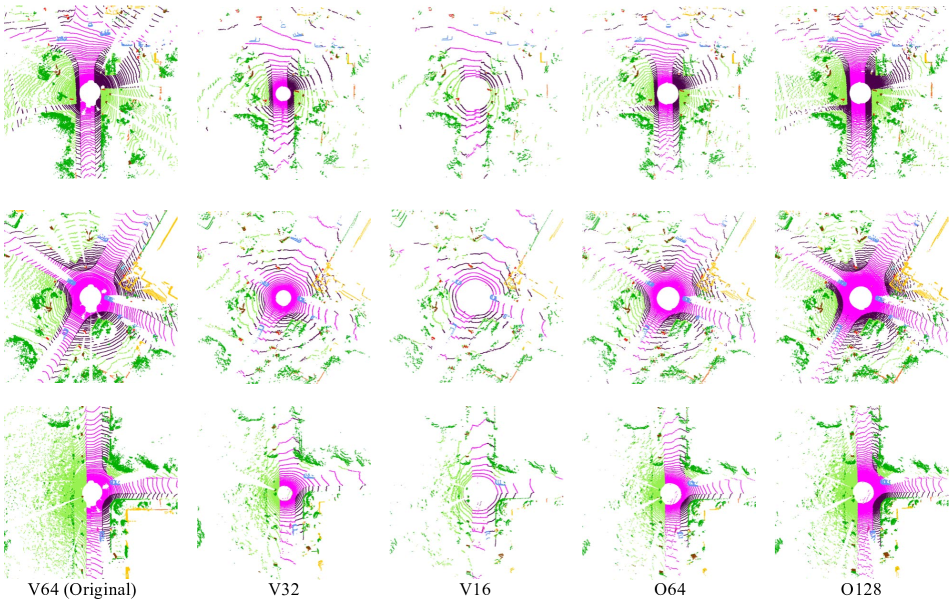
Figure A2: Augmented LiDAR frames using SemanticKITTI dataset. We augment 5 types of LiDARs (Table B). We mark V64 as the original frame because SemanticKITTI is captured with Velodyne HDL-64E.

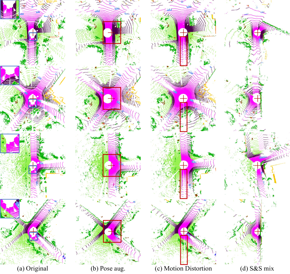
Figure A3: Data augmentation using LiDomAugon SemanticKITTI. (a) Original frames (b) Generated frames after pose augmentation (c) Rendered frames with the consideration of frame distortion (d) Mixed two scenes with various LiDAR configurations. The red cross means the center of the original frames, and the dark red box highlights the changes. Note that the motion distortion exists in the original frames(1st,3rd row: distorted by LiDAR move straight, 2nd row : distorted by LiDAR rotate counter clock-wise, 4th row : distorted by LiDAR rotate counter clock-wise) as the blue box highlighted.

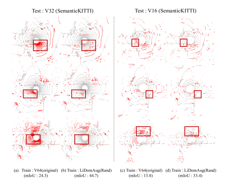
Figure A4: Evaluation of inconsistent LiDAR configuration (corresponds to Table 3 in the main paper). All the models here are trained with/without LiDomAug on SemanticKITTI. The red points indicate the wrong predictions. Train$\rightarrow$Test: (a) V64 (original; w/o LiDomAug)$\rightarrow$V32 (b) LiDomAug$\rightarrow$V32 (c) V64 (original; w/o LiDomAug)$\rightarrow$V16 (d) LiDomAug $\rightarrow$V16. The dark red box highlights the changes. As shown in columns (b) and (d), LiDomAug helps relieve erroneous predictions from inconsistent LiDAR types in training and testing.

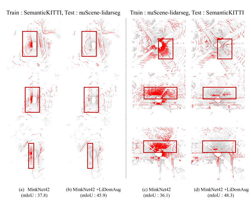
Figure A5: Evaluation on domain adaptation settings with MinkNet42 [Minkowski] backbone (corresponds to Table 1 in main paper). The red points indicate the wrong predictions. Train$\rightarrow$Test: (a) Baseline MinkNet42 (source LiDAR setting V64 $\rightarrow$ target LiDAR setting V32) (b) Trained with our LiDomAug (c) Baseline MinkNet42 (source LiDAR setting V32 $\rightarrow$ target LiDAR setting V64) (d) Trained with our LiDomAug. The dark red box highlights the changes. LiDomAug (b, d) helps to relieve erroneous predictions from dataset shifts in training and testing.

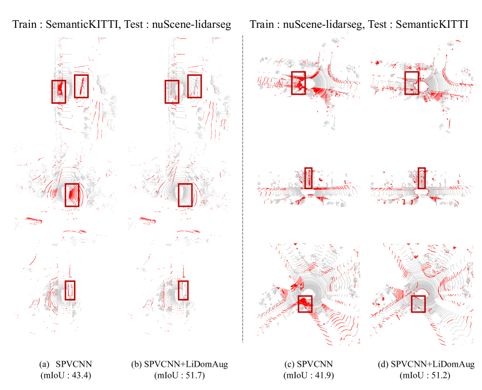
Figure A6: Evaluation on domain adaptation settings with SPVCNN [SPVNAS_ECCV20] backbone (corresponds to Table 5 in main paper). The red points indicate the wrong predictions. Train$\rightarrow$Test: (a) Baseline SPVCNN (source LiDAR setting V64 $\rightarrow$ target LiDAR setting V32) (b) Trained with our LiDomAug (c) Baseline SPVCNN (source LiDAR setting V32 $\rightarrow$ target LiDAR setting V64) (d) Trained with our LiDomAug. The dark red box highlights the changes. LiDomAug (b, d) helps to relieve erroneous predictions from dataset shifts in training and testing.