DiracDiffusion: Denoising and Incremental Reconstruction
with Assured Data-Consistency

Abstract

Diffusion models have established new state of the art in a multitude of computer vision tasks, including image restoration. Diffusion-based inverse problem solvers generate reconstructions of exceptional visual quality from heavily corrupted measurements. However, in what is widely known as the perception-distortion trade-off, the price of perceptually appealing reconstructions is often paid in declined distortion metrics, such as PSNR. Distortion metrics measure faithfulness to the observation, a crucial requirement in inverse problems. In this work, we propose a novel framework for inverse problem solving, namely we assume that the observation comes from a stochastic degradation process that gradually degrades and noises the original clean image. We learn to reverse the degradation process in order to recover the clean image. Our technique maintains consistency with the original measurement throughout the reverse process, and allows for great flexibility in trading off perceptual quality for improved distortion metrics and sampling speedup via early-stopping. We demonstrate the efficiency of our method on different high-resolution datasets and inverse problems, achieving great improvements over other state-of-the-art diffusion-based methods with respect to both perceptual and distortion metrics. Source code and pre-trained models will be released soon.

1 Introduction

Diffusion models are powerful generative models capable of synthesizing samples of exceptional quality by reversing a diffusion process that gradually corrupts a clean image by adding Gaussian noise. Diffusion models have been explored from two perspectives: Denoising Diffusion Probabilistic Models (DDPM) [40, 17] and Score-Based Models [43, 44], which have been recently unified under a general framework of Stochastic Differential Equations (SDEs) [46]. Diffusion models have established new state of the art in image generation [14, 31, 38, 34, 36, 18, 37], audio [28] and video synthesis [19], and recently have been deployed for solving inverse problems with great success.

In inverse problems, one wishes to recover a signal $\bm{x}$ from a noisy observation $\bm{y}$ connected via the forward model $\mathcal{A}$ and measurement noise $\bm{z}$ in the form $\bm{y}=\mathcal{A}(\bm{x})+\bm{z}$. As $\mathcal{A}$ is typically non-invertible, prior knowledge on $x$ has been incorporated in a variety of ways including sparsity-inducing regularizers [4, 15], plug-and-play priors [47] and learned deep learning priors [33]. Diffusion models learn a prior over the data distribution by matching the gradient of the log density (Stein-score). The unconditional score function learned by diffusion models has been successfully leveraged to solve inverse problems without any task-specific training [22, 21, 39]. However, as the score of the posterior distribution is intractable in general, different methods have been proposed to enforce consistency between the generated image and the corresponding observations. These methods include alternating between a step of unconditional update and a step of projection[45, 9, 8] or other correction techniques [6, 7] to guide the diffusion process towards data consistency. Another line of work proposes diffusion in the spectral space of the forward operator, achieving high quality reconstructions, however requires costly singular value decomposition [27, 25, 26]. Concurrent work uses pseudo-inverse guidance [42] to incorporate the model into the reconstruction process. All of these methods utilize a score function learned from denoising score-matching on a standard diffusion process that simply adds Gaussian noise to clean images, and therefore the specific corruption model of the inverse problem is not incorporated into model training directly.

There has been a recent push to broaden the notion of Gaussian diffusion, such as extension to other noise distributions [11, 30, 32]. In the context of image generation, there has been work to generalize the corruption process, such as blur diffusion [29, 20], inverse heat dissipation [35] and arbitrary linear corruptions [10]. [2] questions the necessity of stochasticity in the generative process all together and demonstrates empirical results on noiseless corruptions with arbitrary deterministic degradations. However, designing the diffusion process specifically for inverse problem solving has not been explored extensively yet. A recent example is [49] proposing adding an additional drift term to the forward SDE that pulls the iterates towards the corrupted measurement and demonstrates high quality reconstructions for JPEG compression artifact removal. Concurrent work [12] defines the forward process as convex combinations between the clean image and the corrupted observation, obtaining promising results in motion deblurring and super-resolution.

Despite all of these successes of diffusion models in high-quality image generation, the requirements imposed on inverse problems are very different from synthetic image generation. First, due to the perception-distortion trade-off [3], as diffusion models generate images of exceptional detail, typically reconstruction methods relying on diffusion underperform in distortion metrics, such as PSNR and SSIM [6], that are traditionally used to evaluate image reconstructions. Moreover, as data consistency is not always explicitly enforced during reverse diffusion, we may obtain visually appealing reconstructions, that are in fact not faithful to our original observations.

In this paper, we propose a novel framework for solving inverse problems using a generalized notion of diffusion that mimics the corruption process that produced the observation. We call our method Dirac: Denoising and Incremental Reconstruction with Assured data-Consistency. As the forward model and noising process are directly incorporated into the framework, our method maintains data consistency throughout the reverse diffusion process, without any additional steps such as projections. Furthermore, we make the key observation that details are gradually added to the posterior mean estimates during the sampling process. This property imbues our method with great flexibility: by leveraging early-stopping we can freely trade off perceptual quality for better distortion metrics and sampling speedup or vice versa. We provide theoretical analysis on the accuracy, performance and limitations of our method that are well-supported by empirical results. Our numerical experiments demonstrate state-of-the-art results in terms of both perceptual and distortion metrics with fast sampling.

2 Background

Diffusion models – Diffusion models are generative models based on a corruption process that gradually transforms a clean image distribution $q_{0}$ into a known prior distribution which is tractable, but contains no information of data. The corruption level, or severity as we refer to it in this paper, is indexed by time $t$ and increases from $t=0$ (clean images) to $t=1$ (pure noise). The typical corruption process consists of adding Gaussian noise of increasing magnitude to clean images, that is $q_{t}(\bm{x}_{t}|\bm{x}_{0})\sim\mathcal{N}(\bm{x}_{0},\sigma_{t}^{2}\mathbf{I})$, where $\bm{x}_{0}\sim q_{0}$ is a clean image, and $\bm{x}_{t}$ is the corrupted image at time $t$. By learning to reverse the corruption process, one can generate samples from $q_{0}$ by sampling from a simple noise distribution and running the learned reverse diffusion process from $t=1$ to $t=0$.

Diffusion models have been explored along two seemingly different trajectories. Score-Based Models [43, 44] attempt to learn the gradient of the log likelihood and use Langevin dynamics for sampling, whereas DDPM [40, 17] adopts a variational inference interpretation. More recently, a unified framework based on SDEs [46] has been proposed. Namely, both Score-Based Models and DDPM can be expressed via a Forward SDE in the form $\text{d}\bm{x}=f(\bm{x},t)\text{d}t+g(t)\text{d}\bm{w}$ with different choices of $f$ and $g$. Here $\bm{w}$ denotes the standard Wiener process. This SDE is reversible [1], and the Reverse SDE can be written as

$$\text{d}\bm{x}=[f(\bm{x},t)-g^{2}(t)\nabla_{\bm{x}}\log q_{t}(\bm{x})]\text{d}t+g(t)\text{d}\bar{\bm{w}},$$ (1)

where $\bar{\bm{w}}$ is the standard Wiener process, where time flows in the reverse direction. The true score $\nabla_{\bm{x}}\log q_{t}(\bm{x})$ is approximated by a neural network $s_{\bm{\theta}}(\bm{x}_{t},t)$ from the tractable conditional distribution $q_{t}(\bm{x}_{t}|\bm{x}_{0})$ by minimizing

$$\mathbb{E}_{t\sim U[0,1],(\bm{x}_{0},\bm{x}_{t})}\left[w(t)\left\|s_{\bm{\theta}}(\bm{x}_{t},t)-\nabla_{\bm{x}_{t}}q_{t}(\bm{x}_{t}|\bm{x}_{0})\right\|^{2}\right],$$ (2)

where $(\bm{x}_{0},\bm{x}_{t})\sim q_{0}(\bm{x}_{0})q_{t}(\bm{x}_{t}|\bm{x}_{0})$ and $w(t)$ is a weighting function. By applying different discretization schemes to (1), one can derive various algorithms to simulate the reverse diffusion process for sample generation.

Diffusion Models for Inverse problems – Our goal is to solve a noisy, possibly nonlinear inverse problem

$$\bm{\tilde{y}}=\mathcal{A}(\bm{x}_{0})+\bm{z},~{}\bm{z}\sim\mathcal{N}(\bm{0},\sigma^{2}\textbf{I}),$$ (3)

with $\bm{\tilde{y}},\bm{x}_{0}~{}\in\mathbb{R}^{n}$ and $\mathcal{A}:\mathbb{R}^{n}\rightarrow\mathbb{R}^{n}$. That is, we are interested in solving a reconstruction problem, where we observe a measurement $\bm{\tilde{y}}$ that is known to be produced by applying a non-invertible mapping $\mathcal{A}$ to a ground truth signal $\bm{x}_{0}$ and is corrupted by additive noise $\bm{z}$. We refer to $\mathcal{A}$ as the degradation, and $\mathcal{A}(\bm{x}_{0})$ as a degraded signal. Our goal is to recover $\bm{x}_{0}$ as faithfully as possible, which can be thought of as generating samples from the posterior distribution $q(\bm{x}_{0}|\bm{\tilde{y}})$. However, as information is fundamentally lost in the measurement process in (3), prior information on clean signals needs to be incorporated to make recovery possible. In the classical field of compressed sensing [4], a sparsity-inducing regularizer is directly added to the reconstruction objective. An alternative is to leverage diffusion models as the prior to obtain a reverse diffusion sampler for sampling from the posterior based on (1). Using Bayes rule, the score of the posterior can be written as

$$\nabla_{\bm{x}}\log q_{t}(\bm{x}|\bm{\tilde{y}})=\nabla_{\bm{x}}\log q_{t}(\bm{x})+\nabla_{\bm{x}}\log q_{t}(\bm{\tilde{y}}|\bm{x}),$$ (4)

where the first term can be approximated using score-matching as in (2). On the other hand, the second term cannot be expressed in closed-form in general, and therefore a flurry of activity emerged recently to circumvent computing the likelihood directly. The most prominent approach is to alternate between unconditional update from (1) and some form of projection to enforce consistency with the measurement [45, 9, 8]. In recent work, it has been shown that the projection step may throw the sampling path off the data manifold and therefore additional correction steps are proposed to keep the solver close to the manifold [7, 6].

3 Method

In this work, we propose a novel perspective on solving ill-posed inverse problems. In particular, we assume that our noisy observation $\bm{\tilde{y}}$ results from a process that gradually applies more and more severe degradations to an underlying clean signal.

3.1 Degradation severity

To define severity more rigorously, we appeal to the intuition that given two noiseless, degraded signals $\bm{y}$ and $\bm{y}^{+}$ of a clean signal $\bm{x}_{0}$, then $\bm{y}^{+}$ is corrupted by a more severe degradation than $\bm{y}$, if $\bm{y}$ contains all the information necessary to find $\bm{y}^{+}$ without knowing $\bm{x}_{0}$.

Definition 3.1 (Severity of degradations).

A mapping $\mathcal{A}_{+}:\mathbb{R}^{n}\rightarrow\mathbb{R}^{n}$ is a more severe degradation than $\mathcal{A}:\mathbb{R}^{n}\rightarrow\mathbb{R}^{n}$ if there exists a surjective mapping $\mathcal{G}_{\mathcal{A}\rightarrow\mathcal{A}_{+}}:Image(\mathcal{A})\rightarrow Image(\mathcal{A}_{+})$. That is,

$$\mathcal{A}_{+}(\bm{x}_{0})=\mathcal{G}_{\mathcal{A}\rightarrow\mathcal{A}_{+}}(\mathcal{A}(\bm{x}_{0}))~{}~{}\forall\bm{x}_{0}\in dom(\mathcal{A}).$$

We call $\mathcal{G}_{\mathcal{A}\rightarrow\mathcal{A}_{+}}$ the forward degradation transition function from $\mathcal{A}$ to $\mathcal{A}_{+}$.

Take image inpainting as an example (Fig. 2) and let $\mathcal{A}_{t}$ denote a masking operator that sets pixels to $0$ within a centered box, where the box side length is $l(t)=t\cdot W$, where $W$ is the image width and $t\in[0,1]$. Assume that we have an observation $\bm{y}_{t^{\prime}}=\mathcal{A}_{t^{\prime}}(\bm{x}_{0})$ which is a degradation of a clean image $\bm{x}_{0}$ where a small center square with side length $l(t^{\prime})$ is masked out. Given $\bm{y}_{t^{\prime}}$, without having access to the complete clean image, we can find any other masked version of $\bm{x}_{0}$ where a box with at least side length $l(t^{\prime})$ is masked out. Therefore every other masking operator $\mathcal{A}_{t^{\prime\prime}},~{}t^{\prime}<t^{\prime\prime}$ is a more severe degradation than $\mathcal{A}_{t^{\prime}}$. The forward degradation transition function $\mathcal{G}_{\mathcal{A}_{t^{\prime}}\rightarrow\mathcal{A}_{t^{\prime\prime}}}$ in this case is simply $\mathcal{A}_{t^{\prime\prime}}$. We also note here, that the reverse degradation transition function $\mathcal{H}_{\mathcal{A}_{t^{\prime\prime}}\rightarrow\mathcal{A}_{t^{\prime}}}$ that recovers $\mathcal{A}_{t^{\prime}}(\bm{x}_{0})$ from a more severe degradation $\mathcal{A}_{t^{\prime\prime}}(\bm{x}_{0})$ for any $\bm{x}_{0}$ does not exist in general.

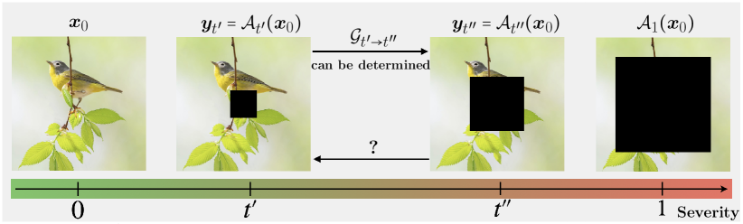
Figure 2: Severity of degradations: We can always find a more degraded image $\bm{y}_{t^{\prime\prime}}$ from a less degraded version of the same clean image $\bm{y}_{t^{\prime}}$ via the forward degradation transition function $\mathcal{G}_{t^{\prime}\rightarrow t^{\prime\prime}}$, but not vice versa.

3.2 Deterministic and stochastic degradation processes

Using this novel notion of degradation severity, we can define a deterministic degradation process that gradually removes information from the clean signal via more and more severe degradations.

Definition 3.2 (Deterministic degradation process).

A deterministic degradation process is a differentiable mapping $\mathcal{A}:[0,1]\times\mathbb{R}^{n}\rightarrow\mathbb{R}^{n}$ that has the following properties:

1. Diminishing severity: $\mathcal{A}(0,\bm{x})=\bm{x}$

2. Monotonically degrading: $\forall t^{\prime}\in[0,1)$ and $t^{\prime\prime}\in(t^{\prime},1]$ $\mathcal{A}(t^{\prime\prime},\cdot)$ is a more severe degradation than $\mathcal{A}(t^{\prime},\cdot)$.

We use the shorthand $\mathcal{A}(t,\cdot)=\mathcal{A}_{t}(\cdot)$ and $\mathcal{G}_{\mathcal{A}_{t^{\prime}}\rightarrow\mathcal{A}_{t^{\prime\prime}}}=\mathcal{G}_{t^{\prime}\rightarrow t^{\prime\prime}}$ for the underlying forward degradation transition functions for all $t^{\prime}<t^{\prime\prime}$.

Our deterministic degradation process starts from a clean signal $\bm{x}_{0}$ at time $t=0$ and applies degradations with increasing severity over time. If we choose $\mathcal{A}(1,\cdot)=\mathbf{0}$, then all information in the original signal is destroyed over the degradation process. One can sample easily from the forward process, that is the process that evolves forward in time, starting from a clean image $\bm{x}_{0}$ at $t=0$. A sample from time $t$ can be computed directly as $\bm{y}_{t}=\mathcal{A}_{t}(\bm{x}_{0})$.

So far we have shown how to write a noiseless measurement $\bm{y}_{t}$ as part of a deterministic degradation process. However, typically our measurements are not only degraded by a non-invertible mapping, but also corrupted by noise as seen in (3). Thus, one can combine the deterministic degradation process with a stochastic noising process that gradually adds Gaussian noise to the degraded measurements.

Definition 3.3 (Stochastic degradation process (SDP)).

$\bm{y}_{t}=\mathcal{A}_{t}(\bm{x}_{0})+\bm{z}_{t},~{}\bm{z}_{t}\sim\mathcal{N}(\bm{0},\sigma_{t}^{2}\textbf{I})$ is a stochastic degradation process if $\mathcal{A}_{t}$ is a deterministic degradation process, $t\in[0,1]$, and $\bm{x}_{0}\sim q_{0}(\bm{x}_{0})$ is a sample from the clean data distribution. We denote the distribution of $\bm{y}_{t}$ as $q_{t}(\bm{y}_{t})\sim\mathcal{N}(\mathcal{A}_{t}(\bm{x}_{0}),\sigma_{t}^{2}\textbf{I})$.

A key contribution of our work is looking at a noisy, degraded signal as a sample from the forward process of an underlying SDP, and considering the reconstruction problem as running the reverse process of the SDP backwards in time in order to recover the clean sample.

3.3 SDP as a Stochastic Differential Equation

We can formulate the evolution of our degraded and noisy measurements $\bm{y}_{t}$ as an SDE:

$$\text{d}\bm{y}_{t}=\dot{\mathcal{A}}_{t}(\bm{x}_{0})\text{d}t+\sqrt{\frac{\text{d}}{\text{d}t}\sigma_{t}^{2}}\text{d}w.$$ (5)

This is an example of an Itô-SDE, and for a fixed $\bm{x}_{0}$ the above process is reversible, where the reverse diffusion process is given by

$$\text{d}\bm{y}_{t}=\left(\dot{\mathcal{A}}_{t}(\bm{x}_{0})\text{d}t-\left(\frac{\text{d}}{\text{d}t}\sigma_{t}^{2}\right)\nabla_{\bm{y}_{t}}\log q_{t}(\bm{y}_{t})\right)\text{d}t+\sqrt{\frac{\text{d}}{\text{d}t}\sigma_{t}^{2}}\text{d}\bar{\bm{w}}.$$ (6)

One would solve the above SDE by discretizing it (for example Euler-Maruyama), approximating differentials with finite differences:

$$\bm{y}_{t-\Delta t}=\bm{y}_{t}+\underbrace{\mathcal{A}_{t-\Delta t}(\bm{x}_{0})-\mathcal{A}_{t}(\bm{x}_{0})}_{\text{incremental reconstruction}}-\underbrace{(\sigma_{t-\Delta_{t}}^{2}-\sigma_{t}^{2})\nabla_{\bm{y}_{t}}\log q_{t}(\bm{y}_{t})}_{\text{denoising}}+\sqrt{\sigma_{t}^{2}-\sigma_{t-\Delta_{t}}^{2}}\bm{z},$$ (7)

where $\bm{z}\sim\mathcal{N}(\bm{0},\textbf{I})$. The update in (7) lends itself to an interesting interpretation. One can look at it as the combination of a small, incremental reconstruction and denoising steps. In particular, assume that ${\bm{y}_{t}=\mathcal{A}_{t}(\bm{x}_{0})+\bm{z}_{t}}$ and let

$$\mathcal{R}(t,\Delta t;\bm{x}_{0}):=\mathcal{A}_{t-\Delta t}(\bm{x}_{0})-\mathcal{A}_{t}(\bm{x}_{0}).$$ (8)

Then, the first term $\bm{y}_{t}+\mathcal{R}(t,\Delta t;\bm{x}_{0})=\mathcal{A}_{t-\Delta t}(\bm{x}_{0})+\bm{z}_{t}$ will reverse a $\Delta t$ step of the deterministic degradation process, equivalent in effect to the reverse degradation transition function $\mathcal{H}_{t\rightarrow t-\Delta t}$. The second term is analogous to a denoising step in standard diffusion, where a slightly less noisy version of the image is predicted. However, before we can simulate the reverse SDE in (7) to recover $\bm{x}_{0}$, we face two obstacles.

Denoising: We do not know the score of $q_{t}(\bm{y}_{t})$. This is commonly tackled by learning a noise-conditioned score network that matches the conditional log-probability $\log q_{t}(\bm{y}_{t}|\bm{x}_{0})$ which we can easily compute. We are also going to follow this path.

Incremental reconstruction: We do not know $\mathcal{A}_{t-\Delta t}(\bm{x}_{0})$ and $\mathcal{A}_{t}(\bm{x}_{0})$ for the incremental reconstruction step, since $\bm{x}_{0}$ is unknown to us when reversing the degradation process (it is in fact what we would like to recover). We are going to address the above issues one-by-one.

3.4 Denoising - learning a score network

To run the reverse SDE, we need the score of the noisy, degraded distribution $\nabla_{\bm{y}_{t}}\log q_{t}(\bm{y}_{t})$, which is intractable. However, we can use the denoising score matching framework to approximate the score. In particular, instead of the true score, we can easily compute the score for the conditional distribution, when the clean image $\bm{x}_{0}$ is given:

$$\nabla_{\bm{y}_{t}}\log q_{t}(\bm{y}_{t}|\bm{x}_{0})=\frac{\mathcal{A}_{t}(\bm{x}_{0})-\bm{y}_{t}}{\sigma_{t}^{2}}.$$ (9)

During training, we have access to clean images $\bm{x}_{0}$ and can generate any degraded, noisy image $\bm{y}_{t}$ using our SDP formulation $\bm{y}_{t}=\mathcal{A}_{t}(\bm{x}_{0})+\bm{z}_{t}$. Thus, we learn an estimator of the conditional score function $s_{\bm{\theta}}(\bm{y}_{t},t)$ by minimizing

$$\mathcal{L}_{t}({\bm{\theta}})=\mathbb{E}_{(\bm{x}_{0},\bm{y}_{t})}\left[\left\|s_{\bm{\theta}}(\bm{y}_{t},t)-\frac{\mathcal{A}_{t}(\bm{x}_{0})-\bm{y}_{t}}{\sigma_{t}^{2}}\right\|^{2}\right],$$ (10)

where $(\bm{x}_{0},\bm{y}_{t})\sim q_{0}(\bm{x}_{0})q_{t}(\bm{y}_{t}|\bm{x}_{0})$. One can show that the well-known result of [48] applies to our SDP formulation, and thus by minimizing the objective in (10), we can learn the score $\nabla_{\bm{y}_{t}}\log q_{t}(\bm{y}_{t})$. The technical condition that all conditional distributions $q_{t}(\bm{y}_{t}|\bm{x}_{0})$ are fully supported requires that we can get to any $\bm{y}_{t}$ from a given $\bm{x}_{0}$ with some non-zero probability, which is achieved by adding Gaussian noise. We include the theorem in the supplementary.

We parameterize the score network as follows:

$$s_{\bm{\theta}}(\bm{y}_{t},t)=\frac{\mathcal{A}_{t}(\Phi_{\bm{\theta}}(\bm{y}_{t},t))-\bm{y}_{t}}{\sigma_{t}^{2}},$$ (11)

that is given a noisy and degraded image as input,the model predicts the underlying clean image $\bm{x}_{0}$. Other parametrizations are also possible, such as predicting $\bm{z}_{t}$ or (equivalently) predicting $\mathcal{A}_{t}(\bm{x}_{0})$. However, as pointed out in [10], this might lead to learning the image distribution only locally, around degraded images. Furthermore, in order to estimate the incremental reconstruction $\mathcal{R}(t,\Delta t;\bm{x}_{0})$, we not only need to estimate $\mathcal{A}_{t}(\bm{x}_{0})$, but other functions of $\bm{x}_{0}$, and thus estimating $\bm{x}_{0}$ directly gives us more flexibility. Rewriting (10) with the new parametrization leads to

$$\mathcal{L}({\bm{\theta}})=\mathbb{E}_{t,(\bm{x}_{0},\bm{y}_{t})}\left[w(t)\left\|\mathcal{A}_{t}(\Phi_{\bm{\theta}}(\bm{y}_{t},t))-\mathcal{A}_{t}(\bm{x}_{0})\right\|^{2}\right],$$ (12)

where ${t\sim U[0,1],(\bm{x}_{0},\bm{y}_{t})\sim q_{0}(\bm{x}_{0})q_{t}(\bm{y}_{t}|\bm{x}_{0})}$ and typical choices in the diffusion literature for the weights $w(t)$ are $1$ or $1/\sigma_{t}^{2}$. Intuitively, the neural network receives a noisy, degraded image, along with the degradation severity, and outputs a prediction $\hat{\bm{x}}_{0}(\bm{y}_{t})=\Phi_{\bm{\theta}}(\bm{y}_{t},t)$ such that the degraded ground truth $\mathcal{A}_{t}(\bm{x}_{0})$ and the degraded prediction $\mathcal{A}_{t}(\hat{\bm{x}}_{0}(\bm{y}_{t}))$ are consistent.

3.5 Incremental reconstructions

Now that we have an estimator of the score, we still need to approximate $\mathcal{R}(t,\Delta t;\bm{x}_{0})$ in order to run the reverse SDE in (7). That is we have to estimate how the degraded image changes if we very slightly decrease the degradation severity. Since we parameterized our score network in (11) to learn a representation of the clean image manifold directly, we can estimate the incremental reconstruction term as

$$\hat{\mathcal{R}}(t,\Delta t;\bm{y}_{t})=\mathcal{A}_{t-\Delta t}(\Phi_{\bm{\theta}}(\bm{y}_{t},t))-\mathcal{A}_{t}(\Phi_{\bm{\theta}}(\bm{y}_{t},t)).$$ (13)

One may consider this a look-ahead method, since we use $\bm{y}_{t}$ with degradation severity $t$ to predict a less severe degradation of the clean image ”ahead” in the reverse process. This becomes more obvious when we note, that our score network already learns to predict $\mathcal{A}_{t}(\bm{x}_{0})$ given $\bm{y}_{t}$ due to the training loss in (12). However, even if we learn the true score perfectly via (12), there is no guarantee that $\mathcal{A}_{t-\Delta t}(\bm{x}_{0})\approx\mathcal{A}_{t-\Delta t}(\Phi_{\bm{\theta}}(\bm{y}_{t},t))$. The following result provides an upper bound on the approximation error.

Theorem 3.4.

Let $\hat{\mathcal{R}}(t,\Delta t;\bm{y}_{t})$ from (13) denote our estimate of the incremental reconstruction, where $\Phi_{\bm{\theta}}(\bm{y}_{t},t)$ is trained on the loss in (12). Let $\mathcal{R}^{*}(t,\Delta t;\bm{y}_{t})=\mathbb{E}[\mathcal{R}(t,\Delta t;\bm{x}_{0})|\bm{y}_{t}]$ denote the MMSE estimator of $\mathcal{R}(t,\Delta t;\bm{x}_{0})$. Assume, that the degradation process is smooth such that $\|\mathcal{A}_{t}(\bm{x})-\mathcal{A}_{t}(\bm{x}^{\prime})\|\leq L_{x}^{(t)}\|\bm{x}-\bm{x}^{\prime}\|,~{}\forall\bm{x},\bm{x}^{\prime}\in\mathbb{R}^{n}$ and $\|\mathcal{A}_{t}(\bm{x})-\mathcal{A}_{t^{\prime}}(\bm{x})\|\leq L_{t}|t-t^{\prime}|,~{}\forall t,t^{\prime}\in[0,1],~{}\forall\bm{x}\in\mathbb{R}^{n}$. Further assume that the clean images have bounded entries $\bm{x}_{0}[i]\leq B,~{}\forall i\in(1,2,...,n)$ and that the error in our score network is bounded by $\|s_{{\bm{\theta}}}(\bm{y}_{t},t)-\nabla_{\bm{y}_{t}}\log q_{t}(\bm{y}_{t})\|\leq\frac{\epsilon_{t}}{\sigma_{t}^{2}},~{}\forall t\in[0,1]$. Then,

$$\|\hat{\mathcal{R}}(t,\Delta t;\bm{y}_{t})-\mathcal{R}^{*}(t,\Delta t;\bm{y}_{t})\|\leq\underbrace{(L_{x}^{(t)}+L_{x}^{(t-\Delta t)})}_{\text{degr. smoothness}}\underbrace{\sqrt{n}B}_{\text{data}}+\underbrace{2L_{t}}_{\text{scheduling}}\underbrace{\Delta t}_{\text{algorithm}}+\underbrace{2\epsilon_{t}}_{\text{optimization}}.$$

The first term in the upper bound depends on the smoothness of the degradation with respect to input images, suggesting that smoother degradations are easier to reconstruct accurately. The second term indicates two crucial points: (1) sharp variations in the degradation with respect to time leads to potentially large estimation error and (2) the error can be controlled by choosing a small enough step size in the reverse process. This provides a possible explanation why masking diffusion models are significantly worse in image generation than models relying on blurring, as observed in [10]. Masking leads to sharp jumps in pixel values at the border of the inpainting mask, thus $L_{t}$ can be arbitrarily large. This can be compensated to a certain degree by choosing a very small $\Delta t$ (very large number of sampling steps), which has also been observed in [10]. Scheduling of the degradation over time is a design parameter, and Theorem 3.4 suggests that sharp changes with respect to $t$ should be avoided. Finally, the error grows with less accurate score estimation, however with large enough network capacity, this term can be driven close to $0$.

The main contributor to the error in Theorem 3.4 stems from the fact that consistency under less severe degradations, that is $\mathcal{A}_{t-\Delta t}(\Phi_{\bm{\theta}}(\bm{y}_{t},t))\approx\mathcal{A}_{t-\Delta t}(\bm{x}_{0})$, is not enforced by the loss in (12). To this end, we propose a novel loss function, the incremental reconstruction loss, that combines learning to denoise and reconstruct simultaneously:

$$\mathcal{L}_{IR}(\Delta t,{\bm{\theta}})=\\ \mathbb{E}_{t,(\bm{x}_{0},\bm{y}_{t})}\left[w(t)\left\|\mathcal{A}_{\tau}(\Phi_{\bm{\theta}}(\bm{y}_{t},t))-\mathcal{A}_{\tau}(\bm{x}_{0})\right\|^{2}\right],$$ (14)

where $\tau=\text{max}(t-\Delta t,0),~{}t\sim U[0,1],$ $(\bm{x}_{0},\bm{y}_{t})\sim q_{0}(\bm{x}_{0})q_{t}(\bm{y}_{t}|\bm{x}_{0})$. It is clear, that minimizing this loss directly improves our estimate of the incremental reconstruction in (13). We find that if $\Phi_{\bm{\theta}}$ has large enough capacity, minimizing the incremental reconstruction loss in (14) also implies minimizing (12), and thus the true score is learned (denoising is achieved). Furthermore, we show that (14) is an upper bound to (12). More details are included in the supplementary. By minimizing (14), the model learns not only to denoise, but also to perform small, incremental reconstructions of the degraded image such that $\mathcal{A}_{t-\Delta t}(\Phi_{\bm{\theta}}(\bm{y}_{t},t))\approx\mathcal{A}_{t-\Delta t}(\bm{x}_{0})$. There is however a trade-off between incremental reconstruction performance and learning the score: we are optimizing an upper bound to (12) and thus it is possible that the score estimation is less accurate. We expect incremental reconstruction loss to work best in scenarios where the degradation may change rapidly with respect to $t$ and hence a network trained to accurately estimate $\mathcal{A}_{t}(\bm{x}_{0})$ from $\bm{y}_{t}$ may become inaccurate when predicting $\mathcal{A}_{t-\Delta t}(\bm{x}_{0})$ from $\bm{y}_{t}$. This hypothesis is further supported by our experiments in Section 4.

3.6 Data consistency

Data consistency is a crucial requirement on generated images when solving inverse problems. That is, we want to obtain reconstructions that are consistent with our original measurement under the degradation model. More formally, we define data consistency as follows in our framework.

Definition 3.5 (Data consistency).

Given a deterministic degradation process $\mathcal{A}_{t}(\cdot)$, two degradation severities $\tau\in[0,1]$ and $\tau^{+}\in[\tau,1]$ and corresponding degraded images $\bm{y}_{\tau}\in\mathbb{R}^{n}$ and $\bm{y}_{\tau^{+}}\in\mathbb{R}^{n}$, $\bm{y}_{\tau^{+}}$ is data consistent with $\bm{y}_{\tau}$ under $\mathcal{A}_{t}(\cdot)$ if $\exists\bm{x}_{0}\in\mathcal{X}_{0}$ such that $\mathcal{A}_{\tau}(\bm{x}_{0})=\bm{y}_{\tau}$ and $\mathcal{A}_{\tau^{+}}(\bm{x}_{0})=\bm{y}_{\tau^{+}}$, where $\mathcal{X}_{0}$ denotes the clean image manifold. We use the notation $\bm{y}_{\tau^{+}}\stackrel{{\scriptstyle\mathclap{\mbox{{{d.c.}}}}}}{{\sim}}\bm{y}_{\tau}$.

Simply put, two degraded images are data consistent, if there is a clean image which may explain both under the deterministic degradation process. As our proposed technique is directly trained to reverse a degradation process, enforcement of data consistency is built-in without applying additional steps, such as projection. The following theorem guarantees that in the ideal scenario, data consistency with the original measurement is maintained in each iteration of the reconstruction algorithm.

Theorem 3.6 (Data consistency over iterations).

Assume that we run the updates in (7) with $s_{\bm{\theta}}(\bm{y}_{t},t)=\nabla_{\bm{y}_{t}}\log q_{t}(\bm{y}_{t}),~{}\forall t\in[0,1]$ and $\hat{\mathcal{R}}(t,\Delta t;\bm{y}_{t})=\mathcal{R}(t,\Delta t;\bm{x}_{0}),~{}\bm{x}_{0}\in\mathcal{X}_{0}$. If we start from a noisy degraded observation $\bm{\tilde{y}}=\mathcal{A}_{1}(\bm{x}_{0})+\bm{z}_{1},~{}\bm{x}_{0}\in\mathcal{X}_{0},~{}\bm{z}_{1}\sim\mathcal{N}(\bm{0},\sigma_{1}^{2}\textbf{I})$ and run the updates in (7) for $\tau=1,1-\Delta t,...,\Delta t,0$, then

$$\mathbb{E}[\bm{\tilde{y}}]\stackrel{{\scriptstyle\mathclap{\mbox{{{d.c.}}}}}}{{\sim}}\mathbb{E}[\bm{y}_{\tau}],~{}\forall\tau\in[1,1-\Delta t,...,\Delta t,0].$$ (15)

Proof is provided in the supplementary. Even though the assumption that we achieve perfect incremental reconstruction is strong, in practice data consistency is indeed maintained without additional guidance from $\bm{\tilde{y}}$ during the reverse process, as shown in Section 4, hinting at the robustness of the proposed framework.

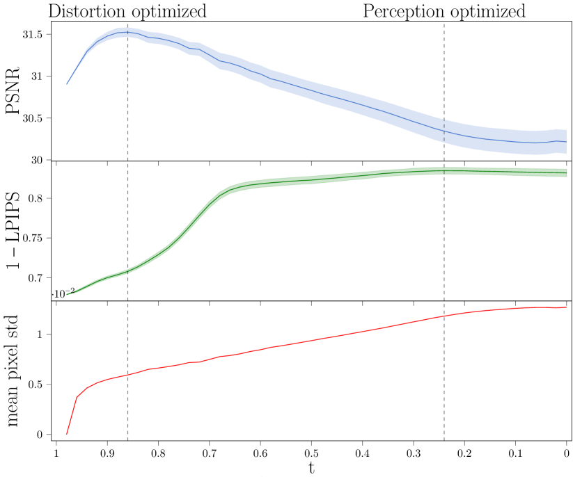
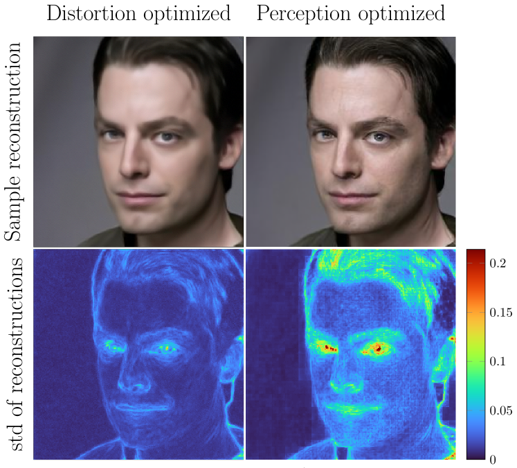
Figure 3: Perception-distortion trade-off on CelebA-HQ deblurring: distortion metrics initially improve, peak fairly early in the reverse process, then gradually deteriorate, while perceptual metrics improve. We plot the mean of $n=30$ trajectories starting from the same initial noisy measurement. The shaded area depicts $\pm std$. We quantify uncertainty via mean pixel-wise standard deviation across different reverse process trajectories . We observe low uncertainty at the distortion peak, with gradual increase during the reverse process. Image regions with fine details correspond to high uncertainty in the final reconstructions.

3.7 Guidance

So far, we have only used our noisy observation $\bm{\tilde{y}}=\mathcal{A}_{1}(\bm{x}_{0})+\bm{z}_{1}$ as a starting point for the reverse diffusion process, however the measurement is not used directly in the update in (7). We learned the score of the prior distribution $\nabla_{\bm{y}_{t}}\log q_{t}(\bm{y}_{t})$, which we can leverage to sample from the posterior distribution $q_{t}(\bm{y}_{t}|\bm{\tilde{y}})$. In fact, using Bayes rule the score of the posterior distribution can be written as

$$\nabla_{\bm{y}_{t}}\log q_{t}(\bm{y}_{t}|\bm{\tilde{y}})=\nabla_{\bm{y}_{t}}\log q_{t}(\bm{y}_{t})+\nabla_{\bm{y}_{t}}\log q_{t}(\bm{\tilde{y}}|\bm{y}_{t}),$$ (16)

where we already approximate $\nabla_{\bm{y}_{t}}\log q_{t}(\bm{y}_{t})$ via $s_{\bm{\theta}}(\bm{y}_{t},t)$. Finding the posterior distribution analytically is not possible, and therefore we use the approximation $q_{t}(\bm{\tilde{y}}|\bm{y}_{t})\approx q_{t}(\bm{\tilde{y}}|\Phi_{\bm{\theta}}(\bm{y}_{t},t)),$ from which distribution we can easily sample from. Since $q_{t}(\bm{\tilde{y}}|\Phi_{\bm{\theta}}(\bm{y}_{t},t))\sim\mathcal{N}(\mathcal{A}_{1}(\Phi_{\bm{\theta}}(\bm{y}_{t},t)),\sigma_{1}^{2}\textbf{I})$, our estimate of the posterior score takes the form

$$s^{\prime}_{\bm{\theta}}(\bm{y}_{t},t)=s_{\bm{\theta}}(\bm{y}_{t},t)-\eta_{t}\nabla_{\bm{y}_{t}}\frac{\|\bm{\tilde{y}}-\mathcal{A}_{1}(\Phi_{\bm{\theta}}(\bm{y}_{t},t))\|^{2}}{2\sigma_{1}^{2}},$$ (17)

where $\eta_{t}$ is a hyperparameter that tunes how much we rely on the original noisy measurement. Even though we do not need to rely on $\bm{\tilde{y}}$ after the initial update for our method to work, we observe small improvements by adding the above guidance scheme to our algorithm.

3.8 Perception-distortion trade-off

Diffusion models generate synthetic images of exceptional quality, almost indistinguishable from real images to the human eye. This perceptual image quality is typically evaluated on features extracted by a pre-trained neural network, resulting in metrics such as Learned Perceptual Image Patch Similarity (LPIPS)[50] or Fréchet Inception Distance (FID)[16]. In image restoration however, we are often interested in image distortion metrics that reflect faithfulness to the original image, such as Peak Signal to Noise Ratio (PSNR) or Structural Similarity Index Measure (SSIM) when evaluating the quality of reconstructions. Interestingly, distortion and perceptual quality are fundamentally at odds with each other, as shown in the seminal work of [3]. As diffusion models tend to favor high perceptual quality, it is often at the detriment of distortion metrics [6].

As shown in Figure 3, we empirically observe that in the reverse process of Dirac, the quality of reconstructions with respect to distortion metrics initially improves, peaks fairly early in the reverse process, then gradually deteriorates. Simultaneously, perceptual metrics such as LPIPS demonstrate stable improvement for most of the reverse process. More intuitively, the algorithm first finds a rough reconstruction that is consistent with the measurement, but lacks fine details. This reconstruction is optimal with respect to distortion metrics, but visually overly smooth and blurry. Consecutively, image details progressively emerge during the rest of the reverse process, resulting in improving perceptual quality at the cost of deteriorating distortion metrics. Therefore, our method provides an additional layer of flexibility: by early-stopping the reverse process, we can trade-off perceptual quality for better distortion metrics. The early-stopping parameter $t_{stop}$ can be tuned on the validation dataset, resulting in distortion- and perception-optimized reconstructions depending on the value of $t_{stop}$.

3.9 Degradation scheduling

In order to deploy our method, we need to define how the degradation changes with respect to severity $t$ following the properties specified in Definition 3.3. That is, we have to determine how to interpolate between the identity mapping $\mathcal{A}_{0}(\bm{x})=\bm{x}$ for $t=0$ and the most severe degradation $\mathcal{A}_{1}(\cdot)$ for $t=1$. Theorem 3.4 suggests that sharp changes in the degradation function with respect to $t$ should be avoided, however we propose a more principled method of scheduling. In particular, we use a greedy algorithm to select a set of degraded distributions, such that the maximum distance between them is minimized. We define the distance between distributions as $\mathbb{E}_{\bm{x}_{0}\sim\mathcal{X}_{0}}[\mathcal{M}(\mathcal{A}_{i}(\bm{x}_{0}),\mathcal{A}_{j}(\bm{x}_{0}))]$, where $\mathcal{M}$ is a pairwise image dissimilarity metric. Details on our scheduling algorithm can be found in the Supplementary. An overview of the complete Dirac algorithm is shown in Algorithm 1.

Algorithm 1 Dirac

$\bm{\tilde{y}}$: noisy observation, $\Phi_{\bm{\theta}}$: score network, $\mathcal{A}_{t}(\cdot)$: degredation function, $\Delta t$: step size, $\sigma_{t}$: noise std at time $t$, $\eta_{t}$: guidance step size, $\forall t\in[0,1]$, $t_{stop}$: early-stopping parameter

$N\leftarrow\lfloor 1/\Delta t\rfloor$

$\bm{y}\leftarrow\bm{\tilde{y}}$

for $i=1\text{ to }N$ do

     $t\leftarrow 1-\Delta t\cdot i$

     if $t\leq t_{stop}$ then $\triangleright$ Early-stopping

         break

     end if

     $\bm{z}\sim\mathcal{N}(0,\sigma_{t}^{2}\mathbf{I})$

     $\hat{\bm{x}}_{0}\leftarrow\Phi_{\bm{\theta}}(\bm{y},t)$ $\triangleright$ Predict posterior mean

     $\bm{y}_{r}\leftarrow\mathcal{A}_{t-\Delta t}(\hat{\bm{x}}_{0})-\mathcal{A}_{t}(\hat{\bm{x}}_{0})$ $\triangleright$ Incremental reconstruction

     $\bm{y}_{d}\leftarrow-\frac{\sigma_{t-\Delta t}^{2}-\sigma_{t}^{2}}{\sigma_{t}^{2}}(\mathcal{A}_{t}(\hat{\bm{x}}_{0})-\bm{y})$ $\triangleright$ Denoising

     $\bm{y}_{g}\leftarrow-(\sigma_{t-\Delta t}^{2}-\sigma_{t}^{2})\nabla_{y}\|\bm{\tilde{y}}-\mathcal{A}_{1}(\hat{\bm{x}}_{0})\|^{2}$ $\triangleright$ Guidance

     $\bm{y}\leftarrow\bm{y}+\bm{y}_{r}+\bm{y}_{d}+\eta_{t}\bm{y}_{g}+\sqrt{\sigma_{t}^{2}-\sigma_{t-\Delta t}^{2}}\bm{z}$

end for

$\bm{y}$ $\triangleright$ Alternatively, output $\hat{\bm{x}}_{0}$

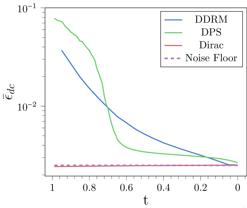
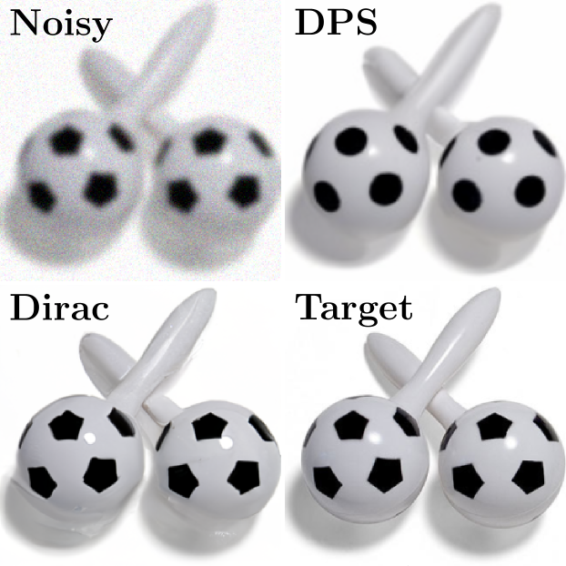
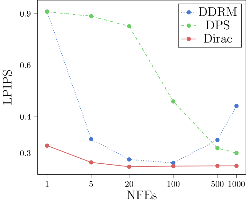
Figure 4: Left: Data consistency curves for FFHQ inpainting. $\epsilon_{dc}:=\left\lVert\bm{\tilde{y}}-\mathcal{A}_{1}(\hat{\bm{x}}_{0}(\bm{y}_{t}))\right\rVert^{2}$ measures how consistent is the clean image estimate with the original noisy measurement. We expect $\epsilon_{dc}$ to approach the noise floor $\sigma_{1}^{2}=0.0025$ in case of perfect data consistency. We plot $\bar{\epsilon}_{dc}$ the mean over the validation set. Dirac maintains data consistency throughout the reverse process. Center: Data consistency is not always achieved with DPS. Right: Number of reverse diffusion steps vs. perceptual quality.

4 Experiments

	Deblurring					Inpainting
Method	PSNR$(\uparrow)$	SSIM$(\uparrow)$	LPIPS$(\downarrow)$	FID$(\downarrow)$		PSNR$(\uparrow)$	SSIM$(\uparrow)$	LPIPS$(\downarrow)$	FID$(\downarrow)$
Dirac-PO (ours)	26.67	0.7418	0.2716	53.36		25.41	0.7595	0.2611	39.43
Dirac-DO (ours)	28.47	0.8054	0.2972	69.15		26.98	0.8435	0.2234	51.87
DPS [6]	25.56	0.6878	0.3008	65.68		21.06	0.7238	0.2899	57.92
DDRM [25]	27.21	0.7671	0.2849	65.84		25.62	0.8132	0.2313	54.37
PnP-ADMM [5]	27.02	0.7596	0.3973	74.17		12.27	0.6205	0.4471	192.36
ADMM-TV	26.03	0.7323	0.4126	89.93		11.73	0.5618	0.5042	264.62

	Deblurring					Inpainting
Method	PSNR$(\uparrow)$	SSIM$(\uparrow)$	LPIPS$(\downarrow)$	FID$(\downarrow)$		PSNR$(\uparrow)$	SSIM$(\uparrow)$	LPIPS$(\downarrow)$	FID$(\downarrow)$
Dirac-PO (ours)	24.68	0.6582	0.3302	53.91		25.48	0.8077	0.2185	40.46
Dirac-DO (ours)	25.76	0.7085	0.3705	83.23		28.42	0.8906	0.1760	40.73
DPS [6]	21.51	0.5163	0.4235	52.60		22.71	0.8026	0.1986	34.55
DDRM [25]	24.53	0.6676	0.3917	61.06		25.92	0.8347	0.2138	33.71
PnP-ADMM [5]	25.02	0.6722	0.4565	98.72		18.14	0.7901	0.2709	101.25
ADMM-TV	24.31	0.6441	0.4578	88.26		17.60	0.7229	0.3157	120.22

Table 1: Experimental results on the FFHQ (top) and ImageNet (bottom) test splits.

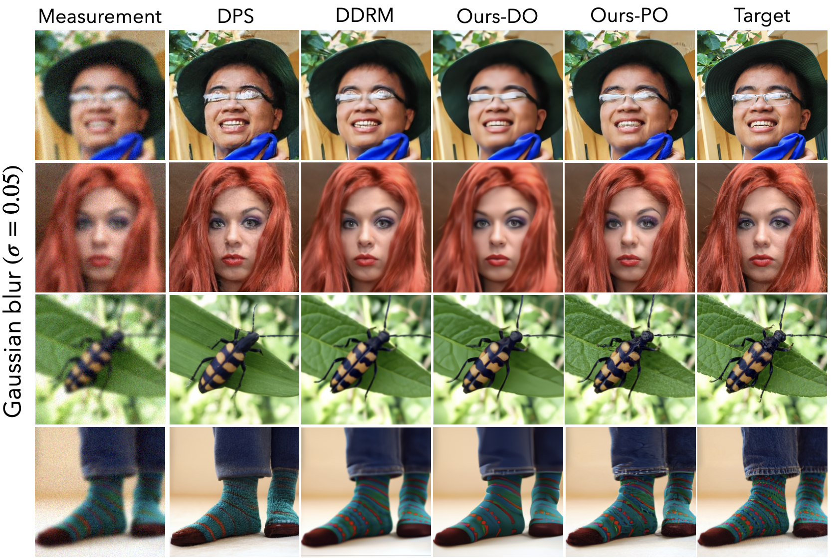
Figure 5: Visual comparison of reconstructions on images from FFHQ (top 2 rows) and ImageNet (bottom 2 rows) on the Gaussian deblurring task.

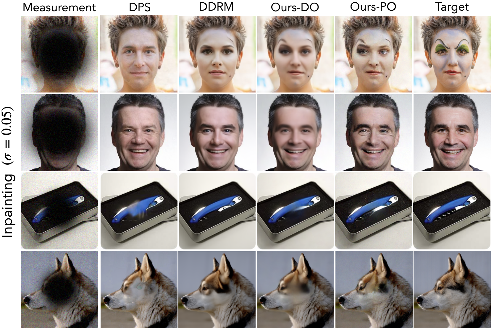
Figure 6: Visual comparison of reconstructions on images from FFHQ (top 2 rows) and ImageNet (bottom 2 rows) on the inpainting task with Gaussian masks.

Experimental setup – We evaluate our method on CelebA-HQ ($256\times 256$) [23] and ImageNet ($256\times 256$) [13]. For competing methods that require a score model, we use pre-trained SDE-VP models. For Dirac, we train models from scratch using the NCSN++[46] architecture. As the pre-trained score-models for competing methods have been trained on the full CelebA-HQ dataset, we test all methods for fair comparison on the first $1k$ images of the FFHQ [24] dataset. For ImageNet experiments, we sample $1$ image from each class from the official validation split to create disjoint validation and test sets of $1k$ images each. We only train our model on the train split of ImageNet.

We investigate two degradation processes of very different properties: Gaussian blur and inpainting, both with additive Gaussian noise. In all cases, noise with $\sigma_{1}=0.05$ is added to the measurements in the $[0,1]$ range. We use standard geometric noise scheduling with $\sigma_{max}=0.05$ and $\sigma_{min}=0.01$ in the SDP. For Gaussian blur, we use a kernel size of $61$, with standard deviation of $w_{max}=3$. We change the standard deviation of the kernel between $w_{max}$(strongest) and $0.3$ (weakest) to parameterize the severity of Gaussian blur in the degradation process, and use the scheduling method described in the supplementary to specify $\mathcal{A}_{t}$. For inpainting, we generate a smooth mask in the form $\left(1-\frac{f(\bm{x};w_{t})}{\max_{\bm{x}}f(\bm{x};w_{t})}\right)^{k}$, where $f(\bm{x};w_{t})$ denotes the density of a zero-mean isotropic Gaussian with standard deviation $w_{t}$ that controls the size of the mask and $k=4$ for sharper transition. We set $w_{1}=50$ for CelebA-HQ/FFHQ inpainting and $30$ for ImageNet inpainting.

We compare our method against DDRM [25], a well-established diffusion-based linear inverse problem solver; DPS [6], a recent, state-of-the-art diffusion technique for noisy inverse problems; PnP-ADMM [5], a reliable traditional solver with learned denoiser; and ADMM-TV, a classical optimization technique. To evaluate performance, we use PSNR and SSIM as distortion metrics and LPIPS and FID as perceptual quality metrics.

Deblurring – We train our model on $\mathcal{L}_{IRN}(\Delta t=0,{\bm{\theta}})$, as we observed no significant difference in using other incremental reconstruction losses, due to the smoothness of the degradation. We show results on our perception-optimized (PO) reconstructions, tuned for best LPIPS and our distortion-optimized (DO) reconstructions, tuned for best PSNR on a separate validation set via early-stopping at the PSNR-peak (see Fig. 3). Our results, summarized in Table 1 (left side), demonstrate superior performance compared with other benchmark methods in terms of both distortion and perceptual metrics. Visual comparison in Figure 5 reveals that DDRM produces reliable reconstructions, similar to our DO images, but these reconstructions tend to lack detail. On the other hand, DPS produces detailed images, similar to our PO reconstructions, but often with hallucinated details inconsistent with the measurement.

Inpainting – We train our model on $\mathcal{L}_{IRN}(\Delta t=1,{\bm{\theta}})$, as we see improvement in reconstruction quality as $\Delta t$ is increased. We hypothesize that this is due to sharp changes in the inpainting operator with respect to $t$, which can be mitigated by the incremental reconstruction loss according to Theorem 3.4. We tuned models to optimize FID, as it is more suitable than pairwise image metrics to evaluate generated image content. Our results in Table 1 (right side) shows best performance in most metrics, followed by DDRM. Fig. 6 shows, that our method generates high quality images even when limited context is available. Ablations on the effect of $\Delta t$ in the incremental reconstruction loss can be found in the supplementary.

Data consistency – Consistency between reconstructions and the original measurement is a crucial requirement in inverse problem solving. Our proposed method has the additional benefit of maintaining data consistency throughout the reverse process, as shown in Theorem 3.6 in the ideal case, however we empirically validate this claim. Figure 4 (left) shows the evolution of $\epsilon_{dc}:=\|\bm{\tilde{y}}-\mathcal{A}_{1}(\hat{\bm{x}}_{0}(\bm{y}_{t}))\|^{2}$, where $\hat{\bm{x}}_{0}(\bm{y}_{t})$ is the clean image estimate at time $t$ ($\Phi_{\bm{\theta}}(\bm{y}_{t},t)$ for our method). Since $\bm{\tilde{y}}=\mathcal{A}_{1}(\bm{x}_{0})+\sigma_{1}^{2}$, we expect $\epsilon_{dc}$ to approach $\sigma_{1}^{2}$ in case of perfect data consistency. We observe that our method, without applying guidance, stays close to the noise floor throughout the reverse process, while other techniques approach data consistency only close to $t=1$. In case of DPS, we observe that data consistency is not always satisfied (see Figure 4, center), as DPS only guides the iterates towards data consistency, but does not directly enforce it. As our technique reverses an SDP, our intermediate reconstructions are always interpretable as degradations of varying severity of the same underlying image. This property allows us to early-stop the reconstruction and still obtain consistent reconstructions.

Sampling speed – Dirac requires low number of reverse diffusion steps for high quality reconstructions leading to fast sampling. Figure 4 (right) compares the perceptual reconstruction quality at different number of reverse diffusion steps for diffusion-based inverse problem solvers. Our method typically requires $20-100$ steps for optimal perceptual quality, and shows the most favorable scaling in the low-NFE regime. Due to early-stopping we can trade-off perceptual quality for better distortion metrics and even further sampling speed-up. We obtain acceptable results even with one-shot reconstruction.

5 Conclusions and limitations

In this paper, we propose a novel framework for solving inverse problems based on reversing a stochastic degradation process. Our solver can flexibly trade off perceptual image quality for more traditional distortion metrics and sampling speedup. Moreover, we show both theoretically and empirically that our method maintains consistency with the measurement throughout the reconstruction process. Our method produces reconstructions of exceptional quality in terms of both perceptual and distortion-based metrics, surpassing comparable state-of-the-art methods on multiple high-resolution datasets and image restoration tasks. The main limitation of our method is that a model needs to be trained from scratch for each inverse problem, whereas other diffusion-based solvers can leverage standard score networks trained via denoising score matching. Incorporating pre-trained score models into our framework for improved speed and reconstruction quality is an interesting direction for future work.

Supplementary material

Appendix A Proofs

A.1 Denoising score-matching guarantee

Just as in standard diffusion, we approximate the score of the noisy, degraded data distribution $\nabla_{\bm{y}_{t}}q_{t}(\bm{y}_{t})$ by matching the score of the tractable conditional distribution $\nabla_{\bm{y}_{t}}q_{t}(\bm{y}_{t}|\bm{x}_{0})$ via minimizing the loss in (12). For standard Score-Based Models with $\mathcal{A}_{t}=\mathbf{I}$, the seminal work of [48] guarantees that the true score is learned by denoising score-matching. More recently, [10] points out that this result holds for a wide range of corruption processes, with the technical condition that the SDP assigns non-zero probability to all $\bm{y}_{t}$ for any given clean image $\bm{x}_{0}$. This condition is satisfied by adding Gaussian noise. For the sake of completeness, we include the theorem from [10] updated with the notation from this paper.

Theorem A.1.

Let $q_{0}$ and $q_{t}$ be two distributions in $\mathbb{R}^{n}$. Assume that all conditional distributions, $q_{t}(\bm{y}_{t}|\bm{x}_{0})$, are supported and differentiable in $\mathbb{R}^{n}$. Let:

$$J_{1}(\theta)=\frac{1}{2}\mathbb{E}_{\bm{y}_{t}\sim q_{t}}\left[\left\lVert\bm{s}_{\theta}(\bm{y}_{t},t)-\nabla_{\bm{y}_{t}}\log q_{t}(\bm{y}_{t})\right\rVert^{2}\right],$$ (18)

$$J_{2}(\theta)=\frac{1}{2}\mathbb{E}_{(\bm{x}_{0},\bm{y}_{t})\sim q_{0}(\bm{x}_{0})q_{t}(\bm{y}_{t}|\bm{x}_{0})}\left[\left\lVert\bm{s}_{\theta}(\bm{y}_{t},t)-\nabla_{\bm{y}_{t}}\log q_{t}(\bm{y}_{t}|\bm{x}_{0})\right\rVert^{2}\right].$$ (19)

Then, there is a universal constant $C$ (that does not depend on $\theta$) such that: $J_{1}(\theta)=J_{2}(\theta)+C$.

The proof, that follows the calculations of [48], can be found in Appendix A.1. of [10]. This result implies that by minimizing the denoising score-matching objective in (19), the objective in (18) is also minimized, thus the true score is learned via matching the tractable conditional distribution $q_{t}(\bm{y}_{t}|\bm{x}_{0})$ governing SDPs.

A.2 Theorem 3.4.

Assumption A.2 (Lipschitzness of degradation).

Assume that $\|\mathcal{A}_{t}(\bm{x})-\mathcal{A}_{t}(\bm{y})\|\leq L_{x}^{(t)}\|\bm{x}-\bm{y}\|,~{}\forall\bm{x},\bm{y}\in\mathbb{R}^{n},~{}\forall t\in[0,1]$ and $\|\mathcal{A}_{t^{\prime}}(\bm{x})-\mathcal{A}_{t^{\prime\prime}}(\bm{x})\|\leq L_{t}|t^{\prime}-t^{\prime\prime}|,~{}\forall\bm{x}\in\mathbb{R}^{n},~{}\forall t^{\prime},t^{\prime\prime}\in[0,1]$.

Assumption A.3 (Bounded signals).

Assume that each entry of clean signals $\bm{x}_{0}$ are bounded as $\bm{x}_{0}[i]\leq B,~{}\forall i\in(1,2,...,n)$.

Lemma A.4.

Assume $\bm{y}_{t}=\mathcal{A}_{t}(\bm{x}_{0})+\bm{z}_{t}$ with $\bm{x}_{0}\sim q_{0}(\bm{x}_{0})$ and $\bm{z}_{t}\sim\mathcal{N}(0,\sigma_{t}^{2}\mathbf{I})$ and that Assumption A.2 holds. Then, the Jensen gap is upper bounded as $\left\lVert\mathbb{E}[\mathcal{A}_{t^{\prime}}(\bm{x}_{0})|\bm{y}_{t}]-\mathcal{A}_{t^{\prime}}(\mathbb{E}[\bm{x}_{0}|\bm{y}_{t}])\right\rVert\leq L_{x}^{(t^{\prime})}\sqrt{n}B,~{}\forall t,t^{\prime}\in[0,1]$.

Proof.

$$\left\lVert\mathbb{E}[\mathcal{A}_{t^{\prime}}(\bm{x}_{0})|\bm{y}_{t}]-\mathcal{A}_{t^{\prime}}(\mathbb{E}[\bm{x}_{0}|\bm{y}_{t}])\right\rVert \stackrel{{\scriptstyle\mathclap{\mbox{{(1)}}}}}{{\leq}}\int\left\lVert\mathcal{A}_{t^{\prime}}(\bm{x}_{0})-\mathcal{A}_{t^{\prime}}(\mathbb{E}[\bm{x}_{0}|\bm{y}_{t}])\right\rVert p(\bm{x}_{0}|\bm{y}_{t})d\bm{x}_{0}$$

$$\stackrel{{\scriptstyle\mathclap{\mbox{{(2)}}}}}{{\leq}}\sqrt{\int\left\lVert\mathcal{A}_{t^{\prime}}(\bm{x}_{0})-\mathcal{A}_{t^{\prime}}(\mathbb{E}[\bm{x}_{0}|\bm{y}_{t}])\right\rVert^{2}p(\bm{x}_{0}|\bm{y}_{t})d\bm{x}_{0}}$$

$$\leq L_{x}^{(t^{\prime})}\sqrt{\int\left\lVert\bm{x}_{0}-\mathbb{E}[\bm{x}_{0}|\bm{y}_{t}]\right\rVert^{2}p(\bm{x}_{0}|\bm{y}_{t})d\bm{x}_{0}}\stackrel{{\scriptstyle\mathclap{\mbox{{(3)}}}}}{{\leq}}L_{x}^{(t^{\prime})}\sqrt{\int\left\lVert\bm{x}_{0}\right\rVert^{2}p(\bm{x}_{0}|\bm{y}_{t})d\bm{x}_{0}}$$

$$\leq L_{x}^{(t^{\prime})}\sqrt{\int nB^{2}p(\bm{x}_{0}|\bm{y}_{t})d\bm{x}_{0}}=L_{x}^{(t^{\prime})}\sqrt{n}B$$

Here $(1)$ and $(2)$ hold due to Jensen’s inequality, and in $(3)$ we use the fact that $\mathbb{E}[\bm{x}_{0}|\bm{y}_{t}]$ is the minimum mean-squared error (MMSE) estimator of $\bm{x}_{0}$, thus we can replace it with $0$ to get an upper bound. ∎

Theorem.

3.4 Let $\hat{\mathcal{R}}(t,\Delta t;\bm{y}_{t})=\mathcal{A}_{t-\Delta t}(\Phi_{\bm{\theta}}(\bm{y}_{t},t))-\mathcal{A}_{t}(\Phi_{\bm{\theta}}(\bm{y}_{t},t))$ denote our estimate of the incremental reconstruction, where $\Phi_{\bm{\theta}}(\bm{y}_{t},t)$ is trained on the loss in $(13)$. Let $\mathcal{R}^{*}(t,\Delta t;\bm{y}_{t})=\mathbb{E}[\mathcal{R}(t,\Delta t;\bm{x}_{0})|\bm{y}_{t}]$ denote the MMSE estimator of $\mathcal{R}(t,\Delta t;\bm{x}_{0})$. If Assumptions A.3 and A.2 hold and the error in our score network is bounded by $\|s_{{\bm{\theta}}}(\bm{y}_{t},t)-\nabla_{\bm{y}_{t}}\log q_{t}(\bm{y}_{t})\|\leq\frac{\epsilon_{t}}{\sigma_{t}^{2}},~{}\forall t\in[0,1]$, then

$$\|\hat{\mathcal{R}}(t,\Delta t;\bm{y}_{t})-\mathcal{R}^{*}(t,\Delta t;\bm{y}_{t})\|\leq\\ (L_{x}^{(t)}+L_{x}^{(t-\Delta t)})\sqrt{n}B+2L_{t}\Delta t+2\epsilon_{t}.$$

Proof.

First, we note that due to Tweedie’s formula,

$$\mathbb{E}[\mathcal{A}_{t}(\bm{x}_{0})|\bm{y}_{t}]=\bm{y}_{t}+\sigma_{t}^{2}\nabla_{\bm{y}_{t}}\log q_{t}(\bm{y}_{t}).$$

Since we parameterized our score model as

$$s_{\bm{\theta}}(\bm{y}_{t},t)=\frac{\mathcal{A}_{t}(\Phi_{\bm{\theta}}(\bm{y}_{t},t))-\bm{y}_{t}}{\sigma_{t}^{2}},$$

the assumption that $\|s_{{\bm{\theta}}}(\bm{y}_{t},t)-\nabla_{\bm{y}_{t}}\log q_{t}(\bm{y}_{t})\|\leq\frac{\epsilon_{t}}{\sigma_{t}^{2}}$, is equivalent to

$$\left\lVert\mathcal{A}_{t}(\Phi_{\bm{\theta}}(\bm{y}_{t},t))-\mathbb{E}[\mathcal{A}_{t}(\bm{x}_{0})|\bm{y}_{t}]\right\rVert\leq\epsilon_{t}.$$ (20)

By applying the triangle inequality repeatedly, and applying Lemma A.4 and (20)

$$\left\lVert\hat{\mathcal{R}}(t,\Delta t;\bm{y}_{t})-\mathcal{R}^{*}(t,\Delta t;\bm{y}_{t})\right\rVert =\left\lVert\left(\mathcal{A}_{t-\Delta t}(\Phi_{\bm{\theta}}(\bm{y}_{t},t))-\mathcal{A}_{t}(\Phi_{\bm{\theta}}(\bm{y}_{t},t))\right)-\left(\mathbb{E}[\mathcal{A}_{t-\Delta t}(\bm{x}_{0})|\bm{y}_{t}]-\mathbb{E}[\mathcal{A}_{t}(\bm{x}_{0})|\bm{y}_{t}]\right)\right\rVert$$

$$\leq\left\lVert\mathcal{A}_{t-\Delta t}(\Phi_{\bm{\theta}}(\bm{y}_{t},t))-\mathbb{E}[\mathcal{A}_{t-\Delta t}(\bm{x}_{0})|\bm{y}_{t}]\right\rVert+\left\lVert\mathcal{A}_{t}(\Phi_{\bm{\theta}}(\bm{y}_{t},t))-\mathbb{E}[\mathcal{A}_{t}(\bm{x}_{0})|\bm{y}_{t}]\right\rVert$$

$$\leq\left\lVert\mathcal{A}_{t-\Delta t}(\Phi_{\bm{\theta}}(\bm{y}_{t},t))-\mathcal{A}_{t-\Delta t}(\mathbb{E}[\bm{x}_{0}|\bm{y}_{t}])+\mathcal{A}_{t-\Delta t}(\mathbb{E}[\bm{x}_{0}|\bm{y}_{t}])-\mathbb{E}[\mathcal{A}_{t-\Delta t}(\bm{x}_{0})|\bm{y}_{t}]\right\rVert+\epsilon_{t}$$

$$\leq\left\lVert\mathcal{A}_{t-\Delta t}(\Phi_{\bm{\theta}}(\bm{y}_{t},t))-\mathcal{A}_{t-\Delta t}(\mathbb{E}[\bm{x}_{0}|\bm{y}_{t}])\right\rVert+L_{x}^{(t-\Delta t)}\sqrt{n}B+\epsilon_{t}$$

$$\leq\left\lVert\mathcal{A}_{t-\Delta t}(\Phi_{\bm{\theta}}(\bm{y}_{t},t))-\mathcal{A}_{t}(\Phi_{\bm{\theta}}(\bm{y}_{t},t))\right\rVert+\left\lVert\mathcal{A}_{t}(\Phi_{\bm{\theta}}(\bm{y}_{t},t))-\mathcal{A}_{t}(\mathbb{E}[\bm{x}_{0}|\bm{y}_{t}])\right\rVert$$

$$\quad+\left\lVert\mathcal{A}_{t}(\mathbb{E}[\bm{x}_{0}|\bm{y}_{t}])-\mathcal{A}_{t-\Delta t}(\mathbb{E}[\bm{x}_{0}|\bm{y}_{t}])\right\rVert+L_{x}^{(t-\Delta t)}\sqrt{n}B+\epsilon_{t}$$

$$\leq\left\lVert\mathcal{A}_{t}(\Phi_{\bm{\theta}}(\bm{y}_{t},t))-\mathcal{A}_{t}(\mathbb{E}[\bm{x}_{0}|\bm{y}_{t}])\right\rVert+2L_{t}\Delta t+L_{x}^{(t-\Delta t)}\sqrt{n}B+\epsilon_{t}$$

$$\leq\left\lVert\mathcal{A}_{t}(\Phi_{\bm{\theta}}(\bm{y}_{t},t))-\mathbb{E}[\mathcal{A}_{t}(\bm{x}_{0})|\bm{y}_{t}]\right\rVert+\left\lVert\mathbb{E}[\mathcal{A}_{t}(\bm{x}_{0})|\bm{y}_{t}]-\mathcal{A}_{t}(\mathbb{E}[\bm{x}_{0}|\bm{y}_{t}])\right\rVert$$

$$\quad+2L_{t}\Delta t+L_{x}^{(t-\Delta t)}\sqrt{n}B+\epsilon_{t}$$

$$\leq 2L_{t}\Delta t+(L_{x}^{(t-\Delta t)}+L_{x}^{(t)})\sqrt{n}B+2\epsilon_{t}.$$

∎

A.3 Incremental reconstruction loss guarantee

Assumption A.5.

The forward degradation transition function $\mathcal{G}_{t^{\prime}\rightarrow t^{\prime\prime}}$ for any $t^{\prime},t^{\prime\prime}\in[0,1],~{}t^{\prime}<t^{\prime\prime}$ is Lipschitz continuous: $\|\mathcal{G}_{t^{\prime}\rightarrow t^{\prime\prime}}(\bm{x})-\mathcal{G}_{t^{\prime}\rightarrow t^{\prime\prime}}(\bm{y})\|\leq L_{G}(t^{\prime},t^{\prime\prime})\|\bm{x}-\bm{y}\|,~{}\forall t^{\prime},t^{\prime\prime}\in[0,1],~{}t^{\prime}<t^{\prime\prime},~{}\forall\bm{x},\bm{y}\in\mathbb{R}^{n}$.

This is a very natural assumption, as we don’t expect the distance between two images after applying a degradation to grow arbitrarily large.

Proposition A.6.

If the model $\Phi_{\bm{\theta}}(\bm{y}_{t},t)$ has large enough capacity, such that $\mathcal{L}_{IR}(\Delta t,{\bm{\theta}})=0$ is achieved, then $s_{\bm{\theta}}(\bm{y}_{t},t)=\nabla_{\bm{y}_{t}}\log q_{t}(\bm{y}_{t}),~{}\forall t\in[0,1]$. Otherwise, if Assumption A.5 holds, then we have

$$\mathcal{L}({\bm{\theta}})\leq\max_{t\in[0,1]}(L_{G}(\tau,t))\mathcal{L}_{IR}(\Delta t,{\bm{\theta}}).$$ (21)

Proof.

We denote $\tau=\max(0,t-\Delta t)$. First, if $\mathcal{L}_{IR}(\Delta t,{\bm{\theta}})=0$, then

$$\mathcal{A}_{\tau}(\Phi_{\bm{\theta}}(\bm{y}_{t},t))=\mathcal{A}_{\tau}(\bm{x}_{0})$$

for all $(\bm{x}_{0},\bm{y}_{t})$ such that $q_{t}(\bm{x}_{0},\bm{y}_{t})>0$. Applying the forward degradation transition function to both sides yields

$$\mathcal{G}_{\tau\rightarrow t}(\mathcal{A}_{\tau}(\Phi_{\bm{\theta}}(\bm{y}_{t},t)))=\mathcal{G}_{\tau\rightarrow t}(\mathcal{A}_{\tau}(\bm{x}_{0})),$$

which is equivalent to

$$\mathcal{A}_{t}(\Phi_{\bm{\theta}}(\bm{y}_{t},t))=\mathcal{A}_{t}(\bm{x}_{0}).$$

This in turn means that $\mathcal{L}({\bm{\theta}})=0$ and thus due to Theorem A.1 the score is learned.

In the more general case,

$$\mathcal{L}({\bm{\theta}}) =\mathbb{E}_{t,(\bm{x}_{0},\bm{y}_{t})}\left[w_{t}\left\|\mathcal{A}_{t}(\Phi_{\bm{\theta}}(\bm{y}_{t},t))-\mathcal{A}_{t}(\bm{x}_{0})\right\|^{2}\right]$$

$$=\mathbb{E}_{t,(\bm{x}_{0},\bm{y}_{t})}\left[w_{t}\left\|\mathcal{G}_{\tau\rightarrow t}(\mathcal{A}_{\tau}(\Phi_{\bm{\theta}}(\bm{y}_{t},t)))-\mathcal{G}_{\tau\rightarrow t}(\mathcal{A}_{\tau}(\bm{x}_{0}))\right\|^{2}\right]$$

$$\leq\mathbb{E}_{t,(\bm{x}_{0},\bm{y}_{t})}\left[w_{t}L_{G}(\tau,t)\left\|\mathcal{A}_{\tau}(\Phi_{\bm{\theta}}(\bm{y}_{t},t))-\mathcal{A}_{\tau}(\bm{x}_{0})\right\|^{2}\right]$$

$$\leq\max_{t\in[0,1]}(L_{G}(\tau,t))\mathbb{E}_{t,(\bm{x}_{0},\bm{y}_{t})}\left[w_{t}\left\|\mathcal{A}_{\tau}(\Phi_{\bm{\theta}}(\bm{y}_{t},t))-\mathcal{A}_{\tau}(\bm{x}_{0})\right\|^{2}\right]$$

$$=\max_{t\in[0,1]}(L_{G}(\tau,t))\mathcal{L}_{IR}(\Delta t,{\bm{\theta}})$$

∎

This means that if the model has large enough capacity, minimizing the incremental reconstruction loss in (14) also implies minimizing (12), and thus the true score is learned (denoising is achieved). Otherwise, the incremental reconstruction loss is an upper bound on the loss in (12). Training a model on (14), the model learns not only to denoise, but also to perform small, incremental reconstructions of the degraded image such that $\mathcal{A}_{t-\Delta t}(\Phi_{\bm{\theta}}(\bm{y}_{t},t))\approx\mathcal{A}_{t-\Delta t}(\bm{x}_{0})$. There is however a trade-off between incremental reconstruction performance and learning the score: as Proposition A.6 indicates, we are optimizing an upper bound to (12) and thus it is possible that the score estimation is less accurate. We expect our proposed incremental reconstruction loss to work best in scenarios where the degradation may change rapidly with respect to $t$ and hence a network trained to accurately estimate $\mathcal{A}_{t}(\bm{x}_{0})$ from $\bm{y}_{t}$ may become inaccurate when predicting $\mathcal{A}_{t-\Delta t}(\bm{x}_{0})$ from $\bm{y}_{t}$. This hypothesis is further supported by our experiments in Section 4. Finally, we mention that in the extreme case where we choose $\Delta t=1$, we obtain a loss function purely in clean image domain.

A.4 Theorem 3.7

Lemma A.7 (Transitivity of data consistency).

If $\bm{y}_{t^{+}}\stackrel{{\scriptstyle\mathclap{\mbox{{{d.c.}}}}}}{{\sim}}\bm{y}_{t}$ and $\bm{y}_{t^{++}}\stackrel{{\scriptstyle\mathclap{\mbox{{{d.c.}}}}}}{{\sim}}\bm{y}_{t+}$ with $t<t^{+}<t^{++}$, then $\bm{y}_{t^{++}}\stackrel{{\scriptstyle\mathclap{\mbox{{{d.c.}}}}}}{{\sim}}\bm{y}_{t}$.

Proof.

By the definition of data consistency $\bm{y}_{t^{++}}\stackrel{{\scriptstyle\mathclap{\mbox{{{d.c.}}}}}}{{\sim}}\bm{y}_{t+}\Rightarrow\exists\bm{x}_{0}:\mathcal{A}_{t^{++}}(\bm{x}_{0})=\bm{y}_{t^{++}}$ and $\mathcal{A}_{t^{+}}(\bm{x}_{0})=y_{t^{+}}$. On the other hand, $y_{t^{+}}\stackrel{{\scriptstyle\mathclap{\mbox{{{d.c.}}}}}}{{\sim}}\bm{y}_{t}\Rightarrow\exists\bm{x}_{0}^{\prime}:\mathcal{A}_{t^{+}}(\bm{x}_{0}^{\prime})=y_{t^{+}}$ and $\mathcal{A}_{t}(\bm{x}_{0}^{\prime})=\bm{y}_{t}$. Therefore,

$$\bm{y}_{t^{++}}=\mathcal{A}_{t^{++}}(\bm{x}_{0})=\mathcal{G}_{t^{+}\rightarrow t^{++}}(\mathcal{A}_{t^{+}}(\bm{x}_{0}))=\mathcal{G}_{t^{+}\rightarrow t^{++}}(\bm{y}_{t^{+}})=\mathcal{G}_{t^{+}\rightarrow t^{++}}(\mathcal{A}_{t^{+}}(\bm{x}_{0}^{\prime}))=\mathcal{A}_{t^{++}}(\bm{x}_{0}^{\prime}).$$

By the definition of data consistency, this implies $\bm{y}_{t^{++}}\stackrel{{\scriptstyle\mathclap{\mbox{{{d.c.}}}}}}{{\sim}}\bm{y}_{t}$. ∎

Theorem.

3.7. Assume that we run the updates in (7) with $s_{\bm{\theta}}(\bm{y}_{t},t)=\nabla_{\bm{y}_{t}}\log q_{t}(\bm{y}_{t}|\bm{x}_{0}),~{}\forall t\in[0,1]$ and $\hat{\mathcal{R}}(t,\Delta t;\bm{y}_{t})=\mathcal{R}(t,\Delta t;\bm{x}_{0}),~{}\bm{x}_{0}\in\mathcal{X}_{0}$. If we start from a noisy degraded observation $\bm{\tilde{y}}=\mathcal{A}_{1}(\bm{x}_{0})+\bm{z}_{1},~{}\bm{x}_{0}\in\mathcal{X}_{0},~{}\bm{z}_{1}\sim\mathcal{N}(\bm{0},\sigma_{1}^{2}\textbf{I})$ and run the updates in (7) for $\tau=1,1-\Delta t,...,\Delta t,0$, then we have

$$\mathbb{E}[\bm{\tilde{y}}]\stackrel{{\scriptstyle\mathclap{\mbox{{{d.c.}}}}}}{{\sim}}\mathbb{E}[\bm{y}_{\tau}],~{}\forall\tau\in[1,1-\Delta t,...,\Delta t,0].$$ (22)

Proof.

Assume that we start from a known measurement $\bm{\tilde{y}}:=\bm{y}_{t}=\mathcal{A}_{t}(\bm{x}_{0})+\bm{z}_{t}$ at arbitrary time $t$ and run reverse diffusion from $t$ with time step $\Delta t$. Starting from $t=1$ that we have looked at in the paper is a subset of this problem. Starting from arbitrary $\bm{y}_{t}$, the first update takes the form

$$\bm{y}_{t-\Delta t} =\bm{y}_{t}+\mathcal{A}_{t-\Delta t}(\Phi_{\bm{\theta}}(\bm{y}_{t},t))-\mathcal{A}_{t}(\Phi_{\bm{\theta}}(\bm{y}_{t},t))-(\sigma_{t-\Delta t}^{2}-\sigma_{t}^{2})\frac{\mathcal{A}_{t}(\Phi_{\bm{\theta}}(\bm{y}_{t},t))-\bm{y}_{t}}{\sigma_{t}^{2}}+\sqrt{\sigma_{t}^{2}-\sigma_{t-\Delta t}^{2}}\bm{z}=$$

$$=\mathcal{A}_{t}(\bm{x}_{0})+\bm{z}_{t}+\mathcal{A}_{t-\Delta t}(\Phi_{\bm{\theta}}(\bm{y}_{t},t))-\mathcal{A}_{t}(\Phi_{\bm{\theta}}(\bm{y}_{t},t))-(\sigma_{t-\Delta t}^{2}-\sigma_{t}^{2})\frac{\mathcal{A}_{t}(\Phi_{\bm{\theta}}(\bm{y}_{t},t))-\mathcal{A}_{t}(\bm{x}_{0})-\bm{z}_{t}}{\sigma_{t}^{2}}$$

$$+\sqrt{\sigma_{t}^{2}-\sigma_{t-\Delta t}^{2}}\bm{z}$$

Due to our assumption on learning the score function, we have $\mathcal{A}_{t}(\Phi_{\bm{\theta}}(\bm{y}_{t},t))=\mathcal{A}_{t}(\bm{x}_{0})$ and due to the perfect incremental reconstruction assumption $\mathcal{A}_{t-\Delta t}(\Phi_{\bm{\theta}}(\bm{y}_{t},t))=\mathcal{A}_{t-\Delta t}(\bm{x}_{0})$. Thus, we have

$$\bm{y}_{t-\Delta t}=\mathcal{A}_{t-\Delta t}(\bm{x}_{0})+\frac{\sigma_{t-\Delta t}^{2}}{\sigma_{t}^{2}}\bm{z}_{t}+\sqrt{\sigma_{t}^{2}-\sigma_{t-\Delta t}^{2}}\bm{z}.$$

Since $z$ and $\bm{z}_{t}$ are independent Gaussian, we can combine the noise terms to yield

$$\bm{y}_{t-\Delta t}=\mathcal{A}_{t-\Delta t}(\bm{x}_{0})+\bm{z}_{t-\Delta t},$$ (23)

with $\bm{z}_{t-\Delta_{t}}\sim\mathcal{N}(\bm{0},\left[\left(\frac{\sigma_{t-\Delta t}^{2}}{\sigma_{t}}\right)^{2}+\sigma^{2}_{t}-\sigma^{2}_{t-\Delta t}\right]\mathbf{I})$. This form is identical to the expression on our original measurement $\bm{\tilde{y}}=\bm{y}_{t}=\mathcal{A}_{t}(\bm{x}_{0})+\bm{z}_{t}$, but with slightly lower degradation severity and noise variance. It is also important to point out that $\mathbb{E}[\bm{y}_{t}]\stackrel{{\scriptstyle\mathclap{\mbox{{{d.c.}}}}}}{{\sim}}\mathbb{E}[\bm{y}_{t-\Delta t}]$. If we repeat the update to find $\bm{y}_{t-2\Delta t}$, we will have the same form as in (23) and $\mathbb{E}[\bm{y}_{t-\Delta t}]\stackrel{{\scriptstyle\mathclap{\mbox{{{d.c.}}}}}}{{\sim}}\mathbb{E}[\bm{y}_{t-2\Delta t}]$. Due to the transitive property of data consistency (Lemma A.7), we also have $\mathbb{E}[\bm{y}_{t}]\stackrel{{\scriptstyle\mathclap{\mbox{{{d.c.}}}}}}{{\sim}}\mathbb{E}[\bm{y}_{t-2\Delta t}]$, that is data consistency is preserved with the original measurement. This reasoning can be then extended for every further update using the transitivity property, therefore we have data consistency in each iteration. ∎

Appendix B Degradation scheduling

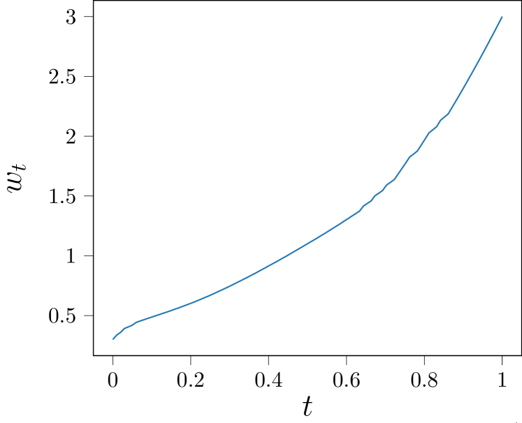
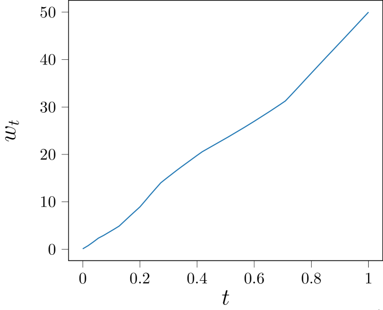
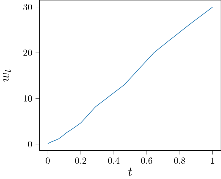
Figure 7: Results of degradation scheduling from Algorithm 2. Left: Gaussian blur with kernel std $w_{t}$ on CelebA-HQ. Center: inpainting with Gaussian mask with kernel width $w_{t}$ on CelebA-HQ. Right: inpainting with Gaussian mask on ImageNet.

When solving inverse problems, we have access to a noisy measurement $\bm{\tilde{y}}=\mathcal{A}(\bm{x}_{0})+\bm{z}$ and we would like to find the corresponding clean image $\bm{x}_{0}$. In order to deploy our method, we need to define how the degradation changes with respect to severity $t$ following the properties specified in Definition 3.3. That is, we have to determine how to interpolate between the identity mapping $\mathcal{A}_{0}(\bm{x})=\bm{x}$ for $t=0$ and the most severe degradation $\mathcal{A}_{1}(\cdot)=\mathcal{A}(\cdot)$ for $t=1$. Theorem 3.4 suggests that sharp changes in the degradation function with respect to $t$ should be avoided, however a more principled method of scheduling is needed.

In the context of image generation, [10] proposes a scheduling framework that splits the path between the distribution of clean images $\mathcal{D}_{0}$ and the distribution of pure noise $\mathcal{D}_{1}$ into $T$ candidate distributions $\mathcal{D}_{i},~{}i\in[1/T,2/T,...,\frac{T-1}{T}]$. Then, they find a path through the candidate distributions that minimizes the total path length, where the distance between $\mathcal{D}_{i}$ and $\mathcal{D}_{j}$ is measured by the Wasserstein-distance. However, for image reconstruction, instead of distance between image distributions, we are more interested in how much a given image degrades in terms of image quality metrics such as PSNR or LPIPS. Therefore, we replace the Wasserstein-distance by a notion of distance between two degradation severities $d(t_{i},t_{j}):=\mathbb{E}_{\bm{x}_{0}\sim\mathcal{D}_{0}}[\mathcal{M}(\mathcal{A}_{t_{i}}(\bm{x}_{0}),\mathcal{A}_{t_{j}}(\bm{x}_{0}))]$, where $\mathcal{M}$ is some distortion-based or perceptual image quality metric that acts on a corresponding pair of images.

We propose a greedy algorithm to select a set of degradations from the set of candidates based on the above notion of dataset-dependent distance, such that the maximum distance is minimized. That is, our scheduler is not only a function of the degradation $\mathcal{A}_{t}$, but also the data. The intuitive reasoning to minimize the maximum distance is that our model has to be imbued with enough capacity to bridge the gap between any two consecutive distributions during the reverse process, and thus the most challenging transition dictates the required network capacity. In particular, given a budget of $m$ intermediate distributions on $[0,1]$, we would like to pick a set of $m$ interpolating severities $\mathcal{S}$ such that

$$\mathcal{S}=arg\min_{\mathcal{T}}\max_{i}d(t_{i},t_{i+1}),$$ (24)

where $\mathcal{T}=\{t_{1},t_{2},...,t_{m}|t_{i}\in[0,1],~{}t_{i}<t_{i+1}~{}\forall i\in(1,2,...,m)\}$ is the set of possible interpolating severities with budget $m$. To this end, we start with $\mathcal{S}=\{0,1\}$ and add new interpolating severities one-by-one, such that the new point splits the interval in $\mathcal{S}$ with the maximum distance. Thus, over iterations the maximum distance is non-increasing. We also have local optimality, as moving a single interpolating severity must increase the maximum distance by the construction of the algorithm. Finally, we use linear interpolation in between the selected interpolating severities. The technique is summarized in Algorithm 2, and we refer the reader to the source code for implementation details.

The results of our proposed greedy scheduling algorithm are shown in Figure 7, where the distance is defined based on the LPIPS metric. In case of blurring, we see a sharp decrease in degradation severity close to $t=1$. This indicates, that LPIPS difference between heavily blurred images is small, therefore most of the diffusion takes place at lower blur levels. On the other hand, we find that inpainting mask size is scaled almost linearly by our algorithm on both datasets we investigated.

Algorithm 2 Greedy Degradation Scheduling

$\mathcal{M}$: pairwise image dissimilarity metric, $\mathcal{X}_{0}$: clean samples, $\mathcal{A}_{t}$: unscheduled degradation function, $N$: number of candidate points, $m$: number of interpolation points

$ts\leftarrow(0,\frac{1}{N-1},\frac{2}{N-1},...,\frac{N-2}{N-1},1)$ $\triangleright$ $N$ candidate severities uniformly distributed over $[0,1]$

$\mathcal{S}\leftarrow(1,N)$ $\triangleright$ Array of indices of output severities in $ts$

$d_{max}\leftarrow Distance(ts[1],ts[N])$ $\triangleright$ Maximum distance between two severities in the output array

$e_{start}\leftarrow 1$ $\triangleright$ Start index of edge with maximum distance

$e_{end}\leftarrow N$ $\triangleright$ End index of edge with maximum distance

for $i=1\text{ to }m$ do

     $s\leftarrow FindBestSplit(e_{start},e_{end},d_{max})$

     $Append(\mathcal{S},s)$

     $d_{max},e_{start},e_{end}\leftarrow UpdateMax(\mathcal{S})$

end for

$\mathcal{S}$

procedure Distance($t_{i},t_{j}$) $\triangleright$ Distance between degradation severities $t_{i}$ and $t_{j}$

     $d\leftarrow\frac{1}{|\mathcal{X}_{0}|}\sum_{x\in\mathcal{X}_{0}}\mathcal{M}(\mathcal{A}_{t_{i}}(x),\mathcal{A}_{t_{j}}(x))$

$d$

end procedure

procedure FindBestSplit($e_{start},e_{end},d_{max}$) $\triangleright$ Split edge into two new edges with minimal maximum distance

     $MaxDistance\leftarrow d_{max}$

     for $j=e_{start}+1\text{ to }e_{end}-1$ do

         $d_{1}\leftarrow Distance(ts[e_{start}],ts[j])$

         $d_{2}\leftarrow Distance(ts[j],ts[e_{end}])$

         if $\max(d_{1},d_{2})<MaxDistance$ then

              $MaxDistance\leftarrow\max(d_{1},d_{2})$

              $Split\leftarrow j$

         end if

     end for

$Split$

end procedure

procedure UpdateMax($\mathcal{S}$)

     $MaxDistance\leftarrow 0$

     for $i=1\text{ to }|S|-1$ do

         $e_{start}\leftarrow\mathcal{S}[i]$

         $e_{end}\leftarrow\mathcal{S}[i+1]$

         $d\leftarrow Distance(ts[e_{start}],ts[e_{end}])$

         if $d>MaxDistance$ then

              $MaxDistance\leftarrow d$

              $NewStart\leftarrow e_{start}$

              $NewEnd\leftarrow e_{end}$

         end if

     end for

$MaxDistance,NewStart,NewEnd$

end procedure

Appendix C Guidance details

Even though Dirac does not need to rely on $\bm{\tilde{y}}$ after the initial update for maintaining data-consistency, we observe small improvements in reconstructions when adding a guidance scheme to our algorithm. As described in Section 3.7, our approximation of the posterior score takes the form

$${s^{\prime}_{\bm{\theta}}(\bm{y}_{t},t)=s_{\bm{\theta}}(\bm{y}_{t},t)-\eta_{t}\nabla_{\bm{y}_{t}}\frac{\|\bm{\tilde{y}}-\mathcal{A}_{1}(\Phi_{\bm{\theta}}(\bm{y}_{t},t))\|^{2}}{2\sigma_{1}^{2}},}$$ (25)

where $\eta_{t}$ is a hyperparameter that tunes how much we rely on the original noisy measurement. For the sake of simplicity, in this discussion we merge the scaling of the gradient into the step size parameter as follows:

$${s^{\prime}_{\bm{\theta}}(\bm{y}_{t},t)=s_{\bm{\theta}}(\bm{y}_{t},t)-\eta_{t}^{\prime}\nabla_{\bm{y}_{t}}\|\bm{\tilde{y}}-\mathcal{A}_{1}(\Phi_{\bm{\theta}}(\bm{y}_{t},t))\|^{2}}$$ (26)

We experiment with two choices of step size scheduling for the guidance term $\eta_{t}^{\prime}$:

• Standard deviation scaled (constant): $\eta_{t}=\eta\frac{1}{2\sigma_{1}^{2}}$, where $\eta$ is a constant hyperparameter and $\sigma_{1}^{2}$ is the noise level on the measurements. This scaling is justified by our derivation of the posterior score approximation, and matches (25).

• Error scaled: $\eta_{t}=\eta\frac{1}{\|\bm{\tilde{y}}-\mathcal{A}_{1}(\Phi_{\bm{\theta}}(\bm{y}_{t},t))\|}$, which has been proposed in [6]. This method attempts to normalize the gradient of the data consistency term.

In general, we find that constant step size works better for deblurring, whereas error scaling performed slightly better for inpainting experiments, however the difference is minor. Figure 8 shows the results of our ablation study on the effect of $\eta_{t}$. We perform deblurring experiments on the CelebA-HQ validation set and plot the mean LPIPS (lower the better) with different step size scheduling methods and varying step size. We see some improvement in LPIPS when adding guidance to our method, however it is not a crucial component in obtaining high quality reconstructions, or for maintaining data-consistency.

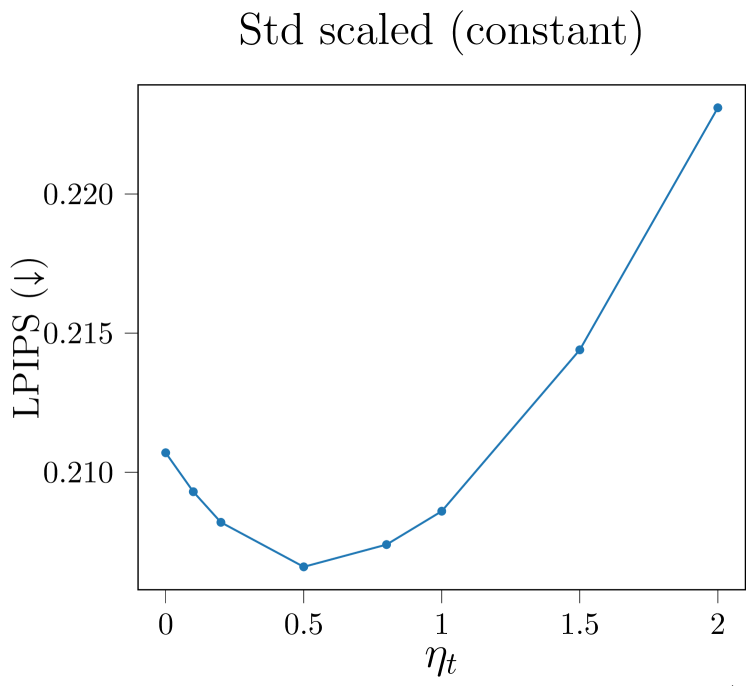
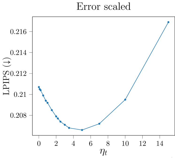
Figure 8: Effect of guidance step size on best reconstruction in terms of LPIPS. We perform experiments on the CelebA-HQ validation set on the deblurring task.

Appendix D Note on the output of the algorithm

In the ideal case, $\sigma_{0}=0$ and $\mathcal{A}_{0}=\mathbf{I}$. However, in practice due to geometric noise scheduling (e.g. $\sigma_{0}=0.01$), there is small magnitude additive noise expected on the final iterate. Moreover, in order to keep the scheduling of the degradation smooth, and due to numerical stability in practice $\mathcal{A}_{0}$ may slightly deviate from the identity mapping close to $t=0$ (for example very small amount of blur). Thus, even close to $t=0$, there may be a gap between the iterates $\bm{y}_{t}$ and the posterior mean estimates $\hat{\bm{x}}_{0}=\Phi_{\theta}(\bm{y}_{t},t)$. Due to these reasons, we observe that in some experiments taking $\Phi_{\theta}(\bm{y}_{t},t)$ as the final output yields better reconstructions. In case of early stopping, taking $\hat{\bm{x}}_{0}$ as the output is instrumental, as an intermediate iterate $\bm{y}_{t}$ represents a sample from the reverse SDP, thus it is expected to be noisy and degraded. However, as $\Phi_{\theta}(\bm{y}_{t},t)$ always predicts the clean image, it can be used at any time step $t$ to obtain an early-stopped prediction of $\bm{x}_{0}$.

Appendix E Experimental details

Datasets – We evaluate our method on CelebA-HQ ($256\times 256$) [23] and ImageNet ($256\times 256$) [13]. For CelebA-HQ training, we use $80\%$ of the dataset for training, and the rest for validation and testing. For ImageNet experiments, we sample $1$ image from each class from the official validation split to create disjoint validation and test sets of $1k$ images each. We only train our model on the official train split of ImageNet. We center-crop and resize ImageNet images to $256\times 256$ resolution. For both datasets, we scale images to $[0,1]$ range.

Comparison methods – We compare our method against DDRM [25], the most well-established diffusion-based linear inverse problem solver; DPS [6], a very recent, state-of-the-art diffusion technique for noisy and possibly nonlinear inverse problems; PnP-ADMM [5], a reliable traditional solver with learned denoiser; and ADMM-TV, a classical optimization technique. More details can be found in Section G.1.

Models – For Dirac, we train new models from scratch using the NCSN++[46] architecture with 67M parameters for all tasks except for ImageNet inpainting, for which we scale the model to 126M parameters. For competing methods that require a score model, we use pre-trained SDE-VP models (126M parameters for CelebA-HQ, 553M parameters for ImageNet). The architectural hyper-parameters for the various score-models can be seen in Table 2.

Training details – We train all models with Adam optimizer, with learning rate $0.0001$ and batch size $32$ on $8\times$ Titan RTX GPUs. We do not use exponential moving averaging or learning rate scheduling schemes. We train for approximately $10M$ examples seen by the network. For the weighting factor $w(t)$ in the loss, we set $w(t)=\frac{1}{\sigma_{t}^{2}}$ in all experiments.

Degradations – We investigate two degradation processes of very different properties: Gaussian blur and inpainting, both with additive Gaussian noise. In all cases, noise with $\sigma_{1}=0.05$ is added to the measurements in the $[0,1]$ range. We use standard geometric noise scheduling with $\sigma_{max}=0.05$ and $\sigma_{min}=0.01$ in the SDP. For Gaussian blur, we use a kernel size of $61$, with standard deviation of $w_{max}=3$ to create the measurements. We change the standard deviation of the kernel between $w_{max}$ (strongest) and $0.3$ (weakest) to parameterize the severity of Gaussian blur in the degradation process, and use the scheduling method described in Section B to specify $\mathcal{A}_{t}$. We keep an imperceptible amount of blur for $t=0$ to avoid numerical instability with very small kernel widths. For inpainting, we generate a smooth mask in the form $\left(1-\frac{f(\bm{x};w_{t})}{\max_{\bm{x}}f(\bm{x};w_{t})}\right)^{k}$, where $f(\bm{x};w_{t})$ denotes the density of a zero-mean isotropic Gaussian with standard deviation $w_{t}$ that controls the size of the mask and $k=4$ for sharper transition. We set $w_{1}=50$ for CelebA-HQ/FFHQ inpainting and $30$ for ImageNet inpainting.

Evaluation method – To evaluate performance, we use PSNR and SSIM as distortion metrics and LPIPS and FID as perceptual quality metrics. For the final reported results, we scale and clip all outputs to the $[0,1]$ range before computing the metrics. We use validation splits to tune the hyper-parameters for all methods, where we optimize for best LPIPS in the deblurring task and for best FID for inpainting. As the pre-trained score-models for competing methods have been trained on the full CelebA-HQ dataset, we test all methods for fair comparison on the first $1k$ images of the FFHQ [24] dataset. The list of test images for ImageNet can be found in the source code.

Sampling hyperparameters – The settings are summarized in Table 3. We tune the reverse process hyper-parameters on validation data. For the interpretation of ’guidance scaling’ we refer the reader to the explanation of guidance step size methods in Section C. In Table 3, ’output’ refers to whether the final reconstruction is the last model output (posterior mean estimate, $\hat{\bm{x}}_{0}=\Phi_{\theta}(\bm{y}_{t},t)$) or the final iterate $\bm{y}_{t}$.

	Dirac(Ours)
Hparam	Deblur/CelebA-HQ	Deblur/ImageNet	Inpainting/CelebA-HQ	Inpainting/ImageNet
model_channels	$128$	$128$	$128$	$128$
channel_mult	$[1,1,2,2,2,2,2]$	$[1,1,2,2,2,2,2]$	$[1,1,2,2,2,2,2]$	$[1,1,2,2,4,4]$
num_res_blocks	$2$	$2$	$2$	$2$
attn_resolutions	$[16]$	$[16]$	$[16]$	$[16]$
dropout	$0.1$	$0.1$	$0.1$	$0.0$
Total # of parameters	67M	67M	67M	126M

	DDRM/DPS
Hparam	Deblur/CelebA-HQ	Deblur/ImageNet	Inpainting/CelebA-HQ	Inpainting/ImageNet
model_channels	$128$	$256$	$128$	$256$
channel_mult	$[1,1,2,2,4,4]$	$[1,1,2,2,4,4]$	$[1,1,2,2,4,4]$	$[1,1,2,2,4,4]$
num_res_blocks	$2$	$2$	$2$	$2$
attn_resolutions	$[16]$	$[32,16,8]$	$[16]$	$[32,16,8]$
dropout	$0.0$	$0.0$	$0.0$	$0.0$
Total # of parameters	126M	553M	126M	553M

Table 2: Architectural hyper-parameters for the score-models for Dirac (top) and other diffusion-based methods (bottom) in our experiments.

	PO Sampling hyper-parameters
Hparam	Deblur/CelebA-HQ	Deblur/ImageNet	Inpainting/CelebA-HQ	Inpainting/ImageNet
$\Delta t$	$0.02$	$0.02$	$0.005$	$0.01$
$t_{stop}$	$0.25$	$0.0$	$0.0$	$0.0$
$\eta_{t}$	$0.5$	$0.2$	$1.0$	$0.0$
Guidance scaling	std	std	error	-
Output	$\hat{\bm{x}}_{0}$	$\hat{\bm{x}}_{0}$	$\bm{y}_{t}$	$\bm{y}_{t}$

	DO Sampling hyper-parameters
Hparam	Deblur/CelebA-HQ	Deblur/ImageNet	Inpainting/CelebA-HQ	Inpainting/ImageNet
$\Delta t$	$0.02$	$0.02$	$0.005$	$0.01$
$t_{stop}$	$0.98$	$0.7$	$0.995$	$0.99$
$\eta_{t}$	$0.5$	$1.5$	$1.0$	$0.0$
Guidance scaling	std	std	error	-
Output	$\hat{\bm{x}}_{0}$	$\hat{\bm{x}}_{0}$	$\hat{\bm{x}}_{0}$	$\hat{\bm{x}}_{0}$

Table 3: Settings for perception optimized (PO) and distortion optimized (DO) sampling for all experiments on test data.

Appendix F Incremental reconstruction loss ablations

We propose the incremental reconstruction loss, that combines learning to denoise and reconstruct simultaneously in the form

$$\mathcal{L}_{IR}(\Delta t,{\bm{\theta}})=\\ \mathbb{E}_{t,(\bm{x}_{0},\bm{y}_{t})}\left[w(t)\left\|\mathcal{A}_{\tau}(\Phi_{\bm{\theta}}(\bm{y}_{t},t))-\mathcal{A}_{\tau}(\bm{x}_{0})\right\|^{2}\right],$$ (27)

where $\tau=\text{max}(t-\Delta t,0),~{}t\sim U[0,1],$ $(\bm{x}_{0},\bm{y}_{t})\sim q_{0}(\bm{x}_{0})q_{t}(\bm{y}_{t}|\bm{x}_{0})$. This loss directly improves incremental reconstruction by encouraging $\mathcal{A}_{t-\Delta t}(\Phi_{\bm{\theta}}(\bm{y}_{t},t))\approx\mathcal{A}_{t-\Delta t}(\bm{x}_{0})$. We show in Proposition A.6 that $\mathcal{L}_{IR}(\Delta t,{\bm{\theta}})$ is an upper bound to the denoising score-matching objective $\mathcal{L}(\bm{\theta})$. Furthermore, we show that given enough model capacity, minimizing $\mathcal{L}_{IR}(\Delta t,{\bm{\theta}})$ also minimizes $\mathcal{L}(\bm{\theta})$. However, if the model capacity is limited compared to the difficulty of the task, we expect a trade-off between incremental reconstruction accuracy and score accuracy. This trade-off might not be favorable in tasks where incremental reconstruction is accurate enough due to the smoothness properties of the degradation (see Theorem 3.4). Here, we perform further ablation studies to investigate the effect of the look-ahead parameter $\Delta t$ in the incremental reconstruction loss.

Deblurring – In case of deblurring, we did not find a significant difference in perceptual quality with different $\Delta t$ settings. Our results on the CelebA-HQ validation set can be seen in Figure 9 (left). We observe that using $\Delta t=0$ (that is optimizing $\mathcal{L}(\bm{\theta})$) yields slightly better reconstructions (difference in the third digit of LPIPS) than optimizing with $\Delta t=1$, that is minimizing

$$\mathcal{L}_{IR}(\Delta t=1,{\bm{\theta}}):=\mathcal{L}_{IR}^{\mathcal{X}_{0}}(\bm{\theta})=\\ \mathbb{E}_{t,(\bm{x}_{0},\bm{y}_{t})}\left[w(t)\left\|\Phi_{\bm{\theta}}(\bm{y}_{t},t)-\bm{x}_{0}\right\|^{2}\right].$$ (28)

This loss encourages one-shot reconstruction and denoising from any degradation severity, intuitively the most challenging task to learn. We hypothesize, that the blur degradation used in our experiments is smooth enough, and thus the incremental reconstruction as per Theorem 3.4 is accurate. Therefore, we do not need to trade off score approximation accuracy for better incremental reconstruction.

Inpainting – We observe very different characteristics in case of inpainting. In fact, using the vanilla score-matching loss $\mathcal{L}(\bm{\theta})$, which is equivalent to $\mathcal{L}_{IR}(\Delta t,{\bm{\theta}})$ with $\Delta t=0$, we are unable to learn a meaningful inpainting model. As we increase the look-ahead $\Delta t$, reconstructions consistently improve. We obtain the best results in terms of FID when minimizing $\mathcal{L}_{IR}^{\mathcal{X}_{0}}(\bm{\theta})$. Our results are summarized in Figure 9 (middle). We hypothesize that due to rapid changes in the inpainting operator, our incremental reconstruction estimator produces very high errors when trained on $\mathcal{L}(\bm{\theta})$ (see Theorem 3.4). Therefore, in this scenario improving incremental reconstruction at the expense of score accuracy is beneficial. Figure 9 (right) demonstrates how reconstructions visually change as we increase the look-ahead $\Delta t$. With $\Delta t=0$, the reverse process misses the clean image manifold completely. As we increase $\Delta t$, reconstruction quality visually improves, but the generated images often have features inconsistent with natural images in the training set. We obtain high quality, detailed reconstructions for $\Delta t=1$ when minimizing $\mathcal{L}_{IR}^{\mathcal{X}_{0}}(\bm{\theta})$.

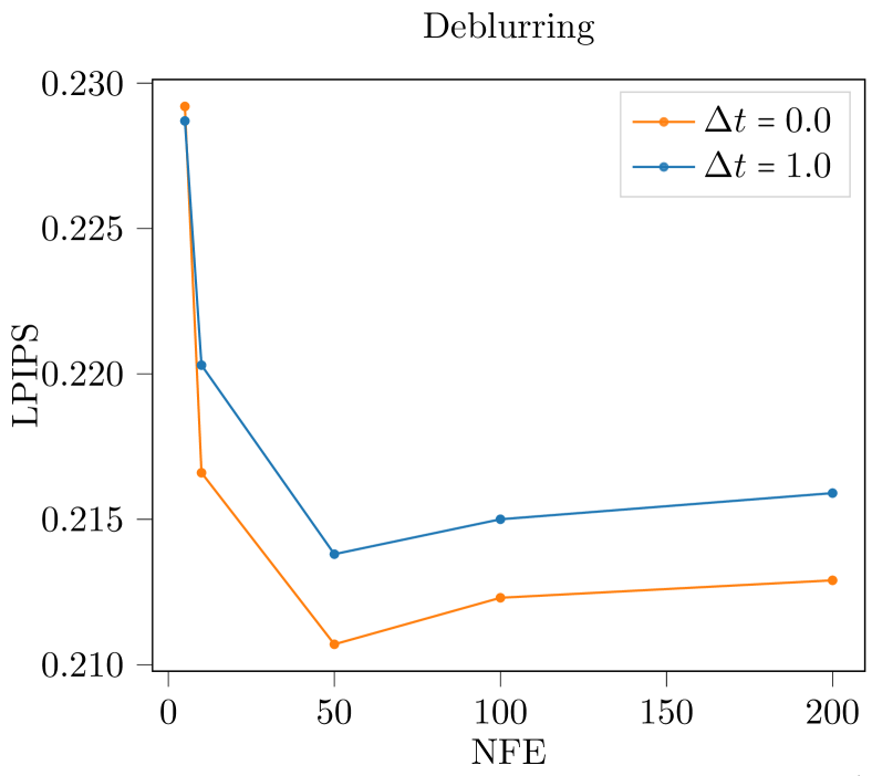
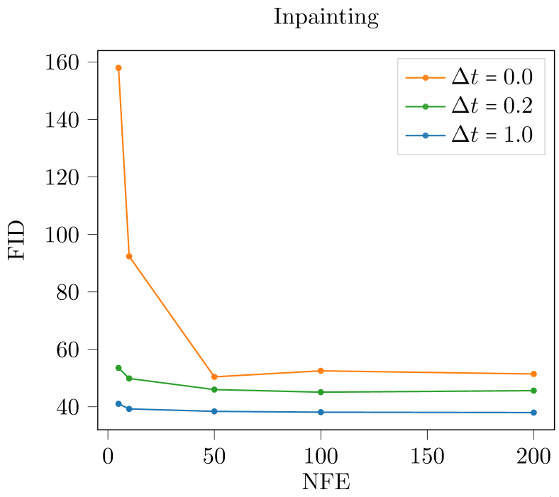
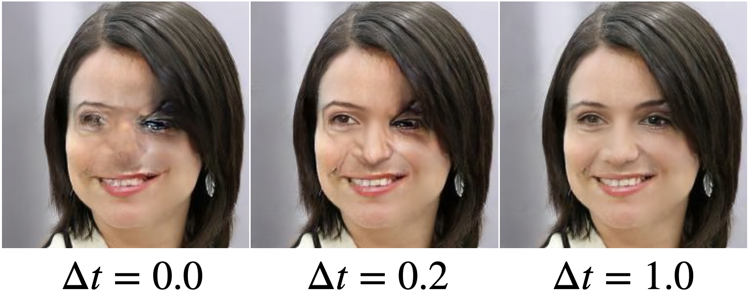
Figure 9: Effect of incremental reconstruction loss step size on the CelebA-HQ validation set for deblurring (left) and inpainting (middle). Visual comparison of inpainted samples is shown on the right.

Appendix G Further incremental reconstruction approximations

In this work, we focused on estimating the incremental reconstruction

$$\mathcal{R}(t,\Delta t;\bm{x}_{0}):=\mathcal{A}_{t-\Delta t}(\bm{x}_{0})-\mathcal{A}_{t}(\bm{x}_{0})$$ (29)

in the form

$$\hat{\mathcal{R}}(t,\Delta t;\bm{y}_{t})=\mathcal{A}_{t-\Delta t}(\Phi_{\bm{\theta}}(\bm{y}_{t},t))-\mathcal{A}_{t}(\Phi_{\bm{\theta}}(\bm{y}_{t},t)),$$ (30)

which we call the look-ahead method. The challenge with this formulation is that we use $\bm{y}_{t}$ with degradation severity $t$ to predict $\mathcal{A}_{t-\Delta t}(\bm{x}_{0})$ with less severe degradation $t-\Delta t$. That is, as we discussed in the paper $\Phi_{\theta}(\bm{y}_{t},t)$ does not only need to denoise images with arbitrary degradation severity, but also has to be able to perform incremental reconstruction, which we address with the incremental reconstruction loss. However, other methods of approximating (29) are also possible, with different trade-offs. The key idea is to use different methods to estimate the gradient of $\mathcal{A}_{t}(\bm{x}_{0})$ with respect to the degradation severity, followed by first-order Taylor expansion to estimate $\mathcal{A}_{t-\Delta t}(\bm{x}_{0})$.

Small look-ahead (SLA) – We use the approximation

$$\mathcal{A}_{t-\Delta t}(\bm{x}_{0})-\mathcal{A}_{t}(\bm{x}_{0})\approx\Delta t\cdot\frac{\mathcal{A}_{t-\delta t}(\bm{x}_{0})-\mathcal{A}_{t}(\bm{x}_{0})}{\delta t},$$ (31)

where $0<\delta t<\Delta t$ to obtain

$$\hat{\mathcal{R}}^{SLA}(t,\Delta t;\bm{y}_{t})=\Delta t\cdot\frac{\mathcal{A}_{t-\delta t}(\Phi_{\bm{\theta}}(\bm{y}_{t},t))-\mathcal{A}_{t}(\Phi_{\bm{\theta}}(\bm{y}_{t},t))}{\delta t}.$$ (32)

The potential benefit of this method is that $\mathcal{A}_{t-\delta t}(\Phi_{\bm{\theta}}(\bm{y}_{t},t))$ may approximate $\mathcal{A}_{t-\delta t}(\bm{x}_{0})$ much more accurately than $\mathcal{A}_{t-\Delta t}(\Phi_{\bm{\theta}}(\bm{y}_{t},t))$ can approximate $\mathcal{A}_{t-\Delta t}(\bm{x}_{0})$, since $t-\delta t$ is closer in severity to $t$ than $t-\Delta t$. However, depending on the sharpness of $\mathcal{A}_{t}$, the first-order Taylor approximation may accumulate large error.

Look-back (LB) – We use the approximation

$$\mathcal{A}_{t-\Delta t}(\bm{x}_{0})-\mathcal{A}_{t}(\bm{x}_{0})\approx\mathcal{A}_{t}(\bm{x}_{0})-\mathcal{A}_{t+\Delta t}(\bm{x}_{0}),$$ (33)

that is we predict the incremental reconstruction based on the most recent change in image degradation. Plugging in our model yields

$$\hat{\mathcal{R}}^{LB}(t,\Delta t;\bm{y}_{t})=\mathcal{A}_{t}(\Phi_{\bm{\theta}}(\bm{y}_{t},t))-\mathcal{A}_{t+\Delta t}(\Phi_{\bm{\theta}}(\bm{y}_{t},t)).$$ (34)

The clear advantage of this formulation over (30) is that if the loss in (12) is minimized such that $\mathcal{A}_{t}(\Phi_{\bm{\theta}}(\bm{y}_{t},t))=\mathcal{A}_{t}(\bm{x}_{0})$, then we also have

$$\mathcal{A}_{t+\Delta t}(\Phi_{\bm{\theta}}(\bm{y}_{t},t))=\mathcal{G}_{t\rightarrow t+\Delta t}(\mathcal{A}_{t}(\Phi_{\bm{\theta}}(\bm{y}_{t},t)))=\mathcal{G}_{t\rightarrow t+\Delta t}(\mathcal{A}_{t}(\bm{x}_{0}))=\mathcal{A}_{t+\Delta t}(\bm{x}_{0}).$$

However, this method may also accumulate large error if $\mathcal{A}_{t}$ changes rapidly close to $t$.

Small look-back (SLB)– Combining the idea in SLA with LB yields the approximation

$$\mathcal{A}_{t-\Delta t}(\bm{x}_{0})-\mathcal{A}_{t}(\bm{x}_{0})\approx\Delta t\cdot\frac{\mathcal{A}_{t}(\bm{x}_{0})-\mathcal{A}_{t+\delta t}(\bm{x}_{0})}{\delta t},$$ (35)

where $0<\delta t<\Delta t$. Using our model, the estimator of the incremental reconstruction takes the form

$$\hat{\mathcal{R}}^{SLB}(t,\Delta t;\bm{y}_{t})=\Delta t\cdot\frac{\mathcal{A}_{t}(\Phi_{\bm{\theta}}(\bm{y}_{t},t))-\mathcal{A}_{t+\delta t}(\Phi_{\bm{\theta}}(\bm{y}_{t},t))}{\delta t}.$$ (36)

Compared with LB, we still have $\mathcal{A}_{t+\delta t}(\Phi_{\bm{\theta}}(\bm{y}_{t},t))=\mathcal{A}_{t+\delta t}(\bm{x}_{0})$ and the error due to first-order Taylor-approximation is reduced, however potentially higher than in case of SLA.

Incremental Reconstruction Network – Finally, an additional model $\phi_{\bm{\theta}^{\prime}}$ can be trained to directly approximate the incremental reconstruction, that is $\phi_{\bm{\theta}^{\prime}}(\bm{y}_{t},t)\approx\mathcal{R}(t,\Delta t;\bm{x}_{0})$. All these approaches are interesting directions for future work.

G.1 Comparison methods

For all methods, hyperparameters are tuned based on first $100$ images of the folder "00001" for FFHQ and tested on the folder "00000". For ImageNet experiments, we use the first samples of the first $100$ classes of ImageNet validation split to tune, last samples of each class as the test set.

G.1.1 DPS

We use the default value of 1000 NFEs for all tasks. We make no changes to the Gaussian blurring operator in the official source code. For inpainting, we copy our operator and apply it in the image input range $[0,1]$. The step size $\zeta^{\prime}$ is tuned via grid search for each task separately based on LPIPS metric. The optimal values are as follows:

1. FFHQ Deblurring: $\zeta^{\prime}=3.0$

2. FFHQ Inpainting: $\zeta^{\prime}=2.0$

3. ImageNet Deblurring: $\zeta^{\prime}=0.3$

4. ImageNet Inpainting: $\zeta^{\prime}=3.0$

As a side note, at the time of writing this paper, the official implementation of DPS adds the noise to the measurement after scaling it to the range $[-1,1]$. For the same noise standard deviation, the effect of the noise is halved as compared to applying in $[0,1]$ range. To compensate for this discrepancy, we set the noise std in the official code to $\sigma=0.1$ for all DPS experiments which is the same effective noise level as $\sigma=0.05$ for our experiments.

G.1.2 DDRM

We keep the default settings $\eta_{B}=1.0$, $\eta=0.85$ for all of the experiments and sample for $20$ NFEs with DDIM [41]. For the Gaussian deblurring task, the linear operator has been implemented via separable 1D convolutions as described in D.5 of DDRM [25]. We note that for blurring task, the operator is applied to the reflection padded input. For Gaussian inpainting task, we set the left and right singular vectors of the operator to be identity ($\textbf{U}=\textbf{V}=\textbf{I}$) and store the mask values as the singular values of the operator. For both tasks, operators are applied to the image in the $[-1,1]$ range.

G.1.3 PnP-ADMM

We take the implementation from the scico library. Specifically the code is modified from the sample notebook. We set the number of ADMM iterations to be maxiter=$12$ and tune the ADMM penalty parameter $\rho$ via grid search for each task based on LPIPS metric. The values for each task are as follows:

1. FFHQ Deblurring: $\rho=0.1$

2. FFHQ Inpainting: $\rho=0.4$

3. ImageNet Deblurring: $\rho=0.1$

4. ImageNet Inpainting: $\rho=0.4$

The proximal mappings are done via pre-trained DnCNN denoiser with 17M parameters.

G.1.4 ADMM-TV

We want to solve the following objective:

$$\operatorname*{arg\,min}_{\bm{x}}\frac{1}{2}\|\bm{y}-\mathcal{A}_{1}(\bm{x})\|_{2}^{2}+\lambda\|\textbf{D}\bm{x}\|_{2,1}$$

where $\bm{y}$ is the noisy degraded measurement, $\mathcal{A}_{1}(\cdot)$ refers to blurring/masking operator and D is a finite difference operator. $\|\textbf{D}\bm{x}\|_{2,1}$ TV regularizes the prediction $\bm{x}$ and $\lambda$ controls the regularization strength. For a matrix $\textbf{A}\in\mathbb{R}^{m\times n}$, the matrix norm $\|.\|_{2,1}$ is defined as:

$$\|\textbf{A}\|_{2,1}=\sum_{i=1}^{m}\sqrt{\sum_{j=1}^{n}\textbf{A}_{ij}^{2}}$$

The implementation is taken from scico library where the code is based on the sample notebook. We note that for consistency, the blurring operator is applied to the reflection padded input. In addition to the penalty parameter $\rho$, we need to tune the regularization strength $\lambda$ in this problem. We tune the pairs $(\lambda,\rho)$ for each task via grid search based on LPIPS metric. Optimal values are as follows:

1. FFHQ Deblurring: $(\lambda,\rho)=(0.007,0.8)$

2. FFHQ Inpainting: $(\lambda,\rho)=(0.02,0.2)$

3. ImageNet Deblurring: $(\lambda,\rho)=(0.007,0.5)$

4. ImageNet Inpainting: $(\lambda,\rho)=(0.02,0.2)$

Appendix H Further reconstruction samples

Here, we provide more samples from Dirac reconstructions on the test split of CelebA-HQ and ImageNet datasets. We visualize the uncertainty of samples via pixelwise standard deviation across $n=10$ generated samples. In experiments where the distortion peak is achieved via one-shot reconstruction, we omit the uncertainty map.

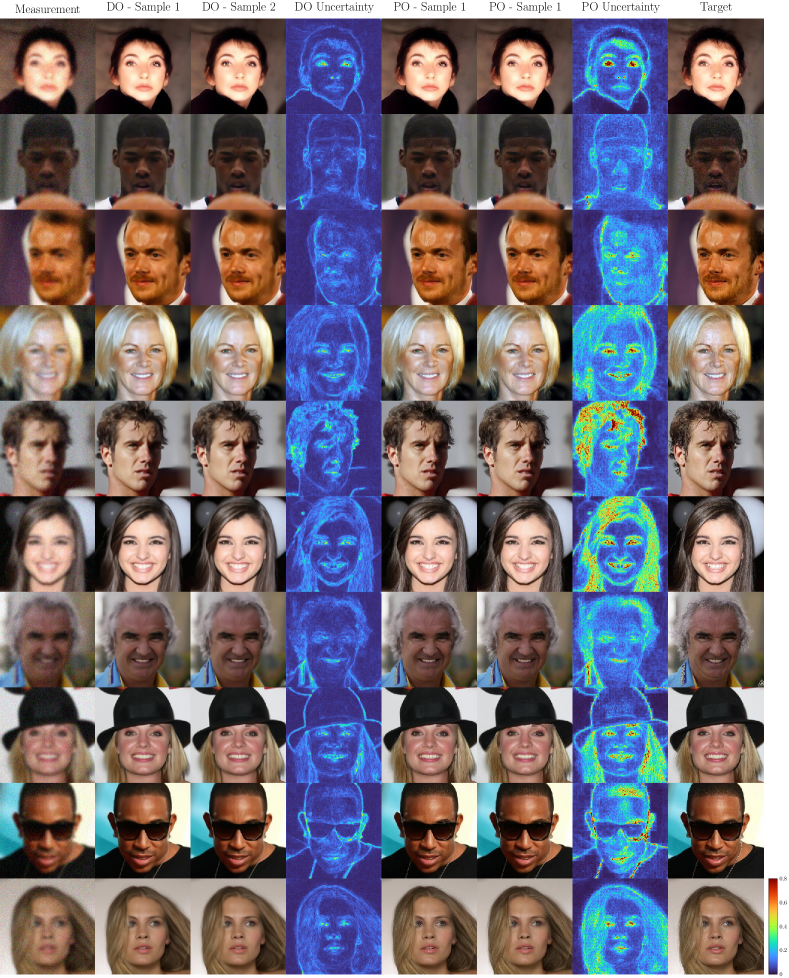
Figure 10: Distortion and Perception optimized deblurring results for the CelebA-HQ dataset (test split). Uncertainty is calculated over $n=10$ reconstructions from the same measurement.

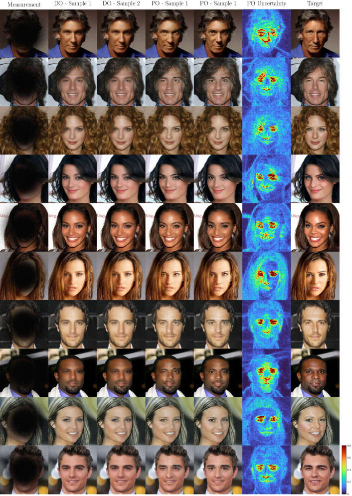
Figure 11: Distortion and Perception optimized inpainting results for the CelebA-HQ dataset (test split). Uncertainty is calculated over $n=10$ reconstructions from the same measurement. For distortion optimized runs, images are generated in one-shot, hence we don’t provide uncertainty maps.

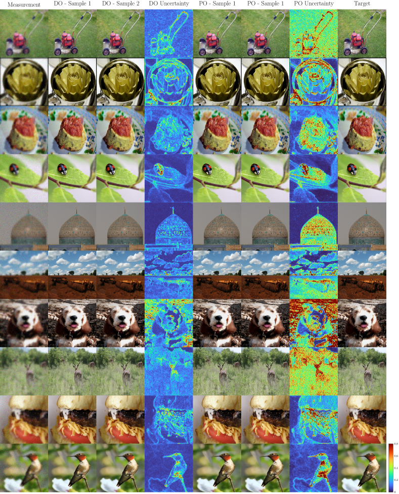
Figure 12: Distortion and Perception optimized deblurring results for the ImageNet dataset (test split). Uncertainty is calculated over $n=10$ reconstructions from the same measurement.

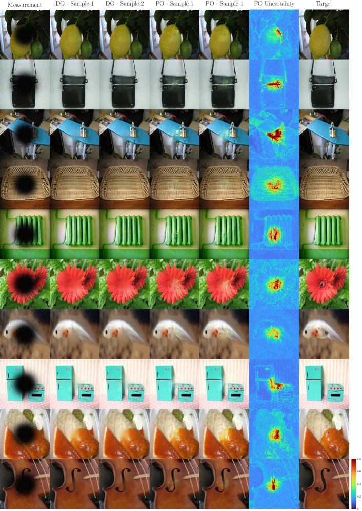
Figure 13: Distortion and Perception optimized inpainting results for the ImageNet dataset (test split). Uncertainty is calculated over $n=10$ reconstructions from the same measurement. For distortion optimized runs, images are generated in one-shot, hence we don’t provide uncertainty maps.

References

- [1] Brian DO Anderson. Reverse-time diffusion equation models. Stochastic Processes and their Applications, 12(3):313–326, 1982.
- [2] Arpit Bansal, Eitan Borgnia, Hong-Min Chu, Jie S Li, Hamid Kazemi, Furong Huang, Micah Goldblum, Jonas Geiping, and Tom Goldstein. Cold diffusion: Inverting arbitrary image transforms without noise. arXiv preprint arXiv:2208.09392, 2022.
- [3] Yochai Blau and Tomer Michaeli. The perception-distortion tradeoff. In Proceedings of the IEEE conference on computer vision and pattern recognition, pages 6228–6237, 2018.
- [4] Emmanuel J. Candes, Justin K. Romberg, and Terence Tao. Stable signal recovery from incomplete and inaccurate measurements. Communications on Pure and Applied Mathematics: A Journal Issued by the Courant Institute of Mathematical Sciences, 59(8):1207–1223, 2006.
- [5] Stanley H Chan, Xiran Wang, and Omar A Elgendy. Plug-and-play admm for image restoration: Fixed-point convergence and applications. IEEE Transactions on Computational Imaging, 3(1):84–98, 2016.
- [6] Hyungjin Chung, Jeongsol Kim, Michael T Mccann, Marc L Klasky, and Jong Chul Ye. Diffusion posterior sampling for general noisy inverse problems. arXiv preprint arXiv:2209.14687, 2022.
- [7] Hyungjin Chung, Byeongsu Sim, Dohoon Ryu, and Jong Chul Ye. Improving diffusion models for inverse problems using manifold constraints. arXiv preprint arXiv:2206.00941, 2022.
- [8] Hyungjin Chung, Byeongsu Sim, and Jong Chul Ye. Come-closer-diffuse-faster: Accelerating conditional diffusion models for inverse problems through stochastic contraction. In Proceedings of the IEEE/CVF Conference on Computer Vision and Pattern Recognition, pages 12413–12422, 2022.
- [9] Hyungjin Chung and Jong Chul Ye. Score-based diffusion models for accelerated mri. Medical Image Analysis, 80:102479, 2022.
- [10] Giannis Daras, Mauricio Delbracio, Hossein Talebi, Alexandros G Dimakis, and Peyman Milanfar. Soft diffusion: Score matching for general corruptions. arXiv preprint arXiv:2209.05442, 2022.
- [11] Jacob Deasy, Nikola Simidjievski, and Pietro Liò. Heavy-tailed denoising score matching. arXiv preprint arXiv:2112.09788, 2021.
- [12] Mauricio Delbracio and Peyman Milanfar. Inversion by direct iteration: An alternative to denoising diffusion for image restoration. arXiv preprint arXiv:2303.11435, 2023.
- [13] Jia Deng, Wei Dong, Richard Socher, Li-Jia Li, Kai Li, and Li Fei-Fei. Imagenet: A large-scale hierarchical image database. In 2009 IEEE conference on computer vision and pattern recognition, pages 248–255. Ieee, 2009.
- [14] Prafulla Dhariwal and Alex Nichol. Diffusion Models Beat GANs on Image Synthesis. arXiv preprint arXiv:2105.05233, 2021.
- [15] David L. Donoho. Compressed sensing. IEEE Transactions on Information Theory, 52(4):1289–1306, 2006.
- [16] Martin Heusel, Hubert Ramsauer, Thomas Unterthiner, Bernhard Nessler, and Sepp Hochreiter. Gans trained by a two time-scale update rule converge to a local nash equilibrium. Advances in neural information processing systems, 30, 2017.
- [17] Jonathan Ho, Ajay Jain, and Pieter Abbeel. Denoising Diffusion Probabilistic Models. arXiv preprint arXiv:2006.11239, 2020.
- [18] Jonathan Ho, Chitwan Saharia, William Chan, David J Fleet, Mohammad Norouzi, and Tim Salimans. Cascaded diffusion models for high fidelity image generation. J. Mach. Learn. Res., 23(47):1–33, 2022.
- [19] Jonathan Ho, Tim Salimans, Alexey Gritsenko, William Chan, Mohammad Norouzi, and David J Fleet. Video diffusion models. arXiv preprint arXiv:2204.03458, 2022.
- [20] Emiel Hoogeboom and Tim Salimans. Blurring diffusion models. arXiv preprint arXiv:2209.05557, 2022.
- [21] Ajil Jalal, Marius Arvinte, Giannis Daras, Eric Price, Alexandros G Dimakis, and Jon Tamir. Robust compressed sensing mri with deep generative priors. Advances in Neural Information Processing Systems, 34:14938–14954, 2021.
- [22] Zahra Kadkhodaie and Eero Simoncelli. Stochastic solutions for linear inverse problems using the prior implicit in a denoiser. Advances in Neural Information Processing Systems, 34:13242–13254, 2021.
- [23] Tero Karras, Timo Aila, Samuli Laine, and Jaakko Lehtinen. Progressive Growing of GANs for Improved Quality, Stability, and Variation. arXiv:1710.10196 [cs, stat], 2018.
- [24] Tero Karras, Samuli Laine, and Timo Aila. A style-based generator architecture for generative adversarial networks. In Proceedings of the IEEE/CVF conference on computer vision and pattern recognition, pages 4401–4410, 2019.
- [25] Bahjat Kawar, Michael Elad, Stefano Ermon, and Jiaming Song. Denoising diffusion restoration models. arXiv preprint arXiv:2201.11793, 2022.
- [26] Bahjat Kawar, Jiaming Song, Stefano Ermon, and Michael Elad. Jpeg artifact correction using denoising diffusion restoration models. arXiv preprint arXiv:2209.11888, 2022.
- [27] Bahjat Kawar, Gregory Vaksman, and Michael Elad. Snips: Solving noisy inverse problems stochastically. Advances in Neural Information Processing Systems, 34:21757–21769, 2021.
- [28] Zhifeng Kong, Wei Ping, Jiaji Huang, Kexin Zhao, and Bryan Catanzaro. Diffwave: A versatile diffusion model for audio synthesis. arXiv preprint arXiv:2009.09761, 2020.
- [29] Sangyun Lee, Hyungjin Chung, Jaehyeon Kim, and Jong Chul Ye. Progressive deblurring of diffusion models for coarse-to-fine image synthesis. arXiv preprint arXiv:2207.11192, 2022.
- [30] Eliya Nachmani, Robin San Roman, and Lior Wolf. Denoising diffusion gamma models. arXiv preprint arXiv:2110.05948, 2021.
- [31] Alex Nichol, Prafulla Dhariwal, Aditya Ramesh, Pranav Shyam, Pamela Mishkin, Bob McGrew, Ilya Sutskever, and Mark Chen. Glide: Towards photorealistic image generation and editing with text-guided diffusion models. arXiv preprint arXiv:2112.10741, 2021.
- [32] Andrey Okhotin, Dmitry Molchanov, Vladimir Arkhipkin, Grigory Bartosh, Aibek Alanov, and Dmitry Vetrov. Star-shaped denoising diffusion probabilistic models. arXiv preprint arXiv:2302.05259, 2023.
- [33] Gregory Ongie, Ajil Jalal, Christopher A. Metzler Richard G. Baraniuk, Alexandros G. Dimakis, and Rebecca Willett. Deep learning techniques for inverse problems in imaging. IEEE Journal on Selected Areas in Information Theory, 2020.
- [34] Aditya Ramesh, Prafulla Dhariwal, Alex Nichol, Casey Chu, and Mark Chen. Hierarchical text-conditional image generation with clip latents. arXiv preprint arXiv:2204.06125, 2022.
- [35] Severi Rissanen, Markus Heinonen, and Arno Solin. Generative modelling with inverse heat dissipation. arXiv preprint arXiv:2206.13397, 2022.
- [36] Robin Rombach, Andreas Blattmann, Dominik Lorenz, Patrick Esser, and Björn Ommer. High-resolution image synthesis with latent diffusion models. In Proceedings of the IEEE/CVF Conference on Computer Vision and Pattern Recognition, pages 10684–10695, 2022.
- [37] Chitwan Saharia, William Chan, Huiwen Chang, Chris Lee, Jonathan Ho, Tim Salimans, David Fleet, and Mohammad Norouzi. Palette: Image-to-image diffusion models. In ACM SIGGRAPH 2022 Conference Proceedings, pages 1–10, 2022.
- [38] Chitwan Saharia, William Chan, Saurabh Saxena, Lala Li, Jay Whang, Emily Denton, Seyed Kamyar Seyed Ghasemipour, Burcu Karagol Ayan, S Sara Mahdavi, Rapha Gontijo Lopes, et al. Photorealistic text-to-image diffusion models with deep language understanding. arXiv preprint arXiv:2205.11487, 2022.
- [39] Chitwan Saharia, Jonathan Ho, William Chan, Tim Salimans, David J. Fleet, and Mohammad Norouzi. Image Super-Resolution via Iterative Refinement. arXiv:2104.07636 [cs, eess], 2021.
- [40] Jascha Sohl-Dickstein, Eric Weiss, Niru Maheswaranathan, and Surya Ganguli. Deep unsupervised learning using nonequilibrium thermodynamics. In International Conference on Machine Learning, pages 2256–2265. PMLR, 2015.
- [41] Jiaming Song, Chenlin Meng, and Stefano Ermon. Denoising diffusion implicit models. In International Conference on Learning Representations, 2021.
- [42] Jiaming Song, Arash Vahdat, Morteza Mardani, and Jan Kautz. Pseudoinverse-guided diffusion models for inverse problems. In International Conference on Learning Representations.
- [43] Yang Song and Stefano Ermon. Generative Modeling by Estimating Gradients of the Data Distribution. arXiv:1907.05600 [cs, stat], 2020.
- [44] Yang Song and Stefano Ermon. Improved Techniques for Training Score-Based Generative Models. arXiv:2006.09011 [cs, stat], 2020.
- [45] Yang Song, Liyue Shen, Lei Xing, and Stefano Ermon. Solving inverse problems in medical imaging with score-based generative models. arXiv preprint arXiv:2111.08005, 2021.
- [46] Yang Song, Jascha Sohl-Dickstein, Diederik P Kingma, Abhishek Kumar, Stefano Ermon, and Ben Poole. Score-based generative modeling through stochastic differential equations. arXiv preprint arXiv:2011.13456, 2020.
- [47] Singanallur V Venkatakrishnan, Charles A Bouman, and Brendt Wohlberg. Plug-and-play priors for model based reconstruction. In 2013 IEEE Global Conference on Signal and Information Processing, pages 945–948. IEEE, 2013.
- [48] Pascal Vincent. A connection between score matching and denoising autoencoders. Neural computation, 23(7):1661–1674, 2011.
- [49] Simon Welker, Henry N Chapman, and Timo Gerkmann. Driftrec: Adapting diffusion models to blind image restoration tasks. arXiv preprint arXiv:2211.06757, 2022.
- [50] Richard Zhang, Phillip Isola, Alexei A Efros, Eli Shechtman, and Oliver Wang. The unreasonable effectiveness of deep features as a perceptual metric. In Proceedings of the IEEE conference on computer vision and pattern recognition, pages 586–595, 2018.