repliclust: Synthetic Data for Cluster Analysis

Abstract

We present repliclust (from replicate and cluster), a Python package for generating synthetic data sets with clusters. Our approach is based on data set archetypes, high-level geometric descriptions from which the user can create many different data sets, each possessing the desired geometric characteristics. The architecture of our software is modular and object-oriented, decomposing data generation into algorithms for placing cluster centers, sampling cluster shapes, selecting the number of data points for each cluster, and assigning probability distributions to clusters. The project webpage, repliclust.org, provides a concise user guide and thorough documentation.

Keywords: Synthetic Data, Simulation, Validation, Clustering, Unsupervised Learning

1 Introduction

Clustering is an important branch of unsupervised learning. The field attempts to uncover hidden structure within data sets. This ambiguous endeavor poses multiple challenges. It is usually not clear what a typical cluster looks like, nor how many clusters a data set contains. In addition, real-world data often exhibits hierarchical structure. Each cluster may contain sub-clusters, raising the possibility of multiple valid clusterings at different resolutions.

This fuzziness can cause headaches for methodologists. When developing a new algorithm for cluster analysis, it is difficult to find appropriate data for testing. One approach is to use data sets from multi-class classification and erase the labels. This practice has limitations since class labels in classification tasks can depend strongly on individual variables, at the expense of the overall structure in the data. Another approach is to use initially unlabeled data that has been annotated by a domain expert. This strategy seems reasonable, though it is not always scalable.

Another possibility is to generate synthetic data on a computer. Surprisingly, in the field of cluster analysis such data possesses several advantages over real data. These include objectivity, manipulability, and fungibility.

First, synthetic data is objective because it is based on mathematical models for data sets with clusters. Such models clarify what a cluster is and how many clusters a data set contains. In addition, a model makes clear how many levels of hierarchy are present in the data.

Second, synthetic data is manipulable because the user can change its properties. Such interventions enable computational experiments. For example, increasing the degree of overlap between clusters allows us to determine how a clustering algorithm performs under challenging conditions.

Third, synthetic data should be fungible. The dictionary defines this word as meaning “replaceable by another identical item.” What we mean is that any individual synthetic data set should be freely replaceable with a fresh data set that has similar overall characteristics. In other words, fungibility requires the ability to sample from the data-generating probability distribution. In the context of synthetic data with clusters, fresh data sets should have new cluster locations and shapes. Consequently, “handcrafted” synthetic data with manually selected cluster locations is not fungible. Fungible synthetic data promotes reproducibility because researchers can share the data-generating probability distributions underlying benchmarks and computational experiments. Our data generator repliclust achieves fungibility by stochastically modeling the geometric structure of a clustered data set, including cluster shapes, locations, sample sizes, and distributions.

In the next section, we describe prior work on synthetic data for cluster analysis.

1.1 Related Work

Most existing data generators for cluster analysis use probabilistic mixture models to generate blob-like ellipsoidal clusters. Perhaps the most important requirement of such generators is the ability to effectively control the separation between clusters while allowing diverse cluster shapes (ellipsoids of varying sizes, eccentricities, and orientations) within a single data set. This requirement often presents a trade-off, as the coexistence of diverse cluster shapes makes it more difficult to manage overlap between clusters.

Different generators navigate this trade-off differently. The HAWKS generator of Shand et al. (2019) uses a genetic algorithm to synthesize data sets of a desired silhouette width. This classical metric goes back to the work of Rousseeuw (1987) and measures the degree of clustering in a data set. High values indicate well-separated clusters, whereas low levels indicate overlap between clusters. The silhouette width presents a promising difficulty scale for benchmarking clustering algorithms, as Shand et al. (2019) discuss. However, its numerical values are difficult to interpret geometrically. In addition, HAWKS’ focus on optimizing the silhouette width makes it lose geometric flexibility. Whereas our method controls cluster shape independently of cluster separation, HAWKS automatically “evolves” cluster means and covariance matrices in order to tune the silhouette width. At a fixed level of cluster separation, the user cannot exert much control over the shapes of clusters.

The generator of Qiu and Joe (2006a) introduces a similar dependence between cluster separation and shape. Their method controls overlap between clusters via a separation index. This quantity, proposed by the same authors, measures the spatial extent of clusters by their extreme quantiles along a one-dimensional projection. The method identifies the direction that best separates two clusters and measures separation along it. Placement of cluster centers takes place deterministically. The generator locates new centers at the vertices of axis-aligned regular simplices translated along the first coordinate axis. To make sufficient room for larger clusters, the method lengthens edges of the simplicial scaffold until all clusters are sufficiently well-separated. To attain a desired separation index exactly, the generator iteratively shrinks the cluster most separated from the others. Hence, it is not possible to control cluster volume without affecting cluster separation.

The generator MDCGen of Iglesias et al. (2019) presents yet another approach to controlling overlap between clusters. Their method initially places cluster centers at the vertices of a rectangular grid. Later on, the algorithm randomly translates cluster centers to make the overall layout less regular. To achieve a desired level of separation between clusters, the user must specify the grid resolution in relation to the cluster sizes. Unfortunately, an axis-aligned rectangular grid is not naturally adapted to the geometry of oblong ellipsoidal clusters at random orientations. While it is possible for obliquely-oriented ellipsoids to fit inside (large) axis-aligned boxes, this approach does not represent their spatial outlines effectively.

Other cluster generators include work by Pei and Zaïane (2006), Handl and Knowles (2005), and Schubert and Zimek (2019). These generators are compelling early contributions but, compared with other methods, appear limited today. The generator of Pei and Zaïane (2006) samples data sets with a user-specified complexity but can only create two-dimensional data sets. The “Gaussian” and “Ellipsoid” generators proposed by Handl and Knowles (2005) generate multivariate Gaussian and ellipsoidal clusters subject to significant restrictions on cluster shapes and overlaps. For example, the “Gaussian” generator ties cluster shape (spherical vs oblong) to the dimensionality, rather than letting the user control it. By contrast, the “Ellipsoid” generator creates oblong clusters of varying eccentricities, but only with circular cross-sections. Neither generator confers the ability to control cluster volume independently of shape. In addition, both generators minimize overlap between clusters, rather than letting the user specify a desired level of overlap.

The ELKI data mining toolkit by Schubert and Zimek (2019) contains an XML-based data generator capable of synthesizing data sets with clusters. However, this generator is not directly comparable to our method, as the user must manually configure all cluster parameters, including the locations of the centers.

Data generation with repliclust (headquartered at repliclust.org) differs from existing approaches in three important ways. First, our generator solicits user input in the form of high-level geometric archetypes. Each archetype acts as a random sampler for probabilistic mixture models, allowing the user to generate similar but different synthetic data sets. Second, we define pairwise cluster overlap in terms of the error rate of the best linear classifier, for which a good approximation is available when clusters are normally distributed. The resulting metric ties overlap between clusters to the expected clustering performance, while naturally adapting to discrepancies in cluster shapes and orientations. Third, our software decomposes data generation into four distinct steps: generating cluster shapes, placing cluster centers, choosing the number of data points for each cluster, and assigning cluster-specific probability distributions. This approach controls different geometric attributes independently from each other, maximizing user control while allowing researchers to adapt the implementation of individual steps without affecting others.

1.2 Outline

The paper is structured as follows. In Section 2, we give an overview of data generation with geometric archetypes. Section 3 details the mathematical model for clusters and probabilistic mixture models used internally in repliclust; this section does not relate to user input but instead gives clarity on the flexibility and limitations of our underlying cluster model. Section 4 explains how a user specifies a geometric archetype. Next, Section 5 introduces our definition of cluster overlap and describes an optimization-based framework to manage it. Subsequently, Section 6 describes repliclust’s modular software architecture.

Having revealed the basic workings of repliclust at this point, in Section 7 we verify empirically that our definition of overlap correlates strongly with the empirical clustering performance. In addition, a small benchmark comparing the performance of the K-Means and Gaussian mixture clustering algorithms illustrates the utility of our data generator. In contrast to conventional benchmarks, repliclust allows us to tally performance by data set archetype, yielding fine-grained insights into the strengths and weaknesses of each clustering algorithm. Finally, in Section 8 we summarize the main ideas in this paper and give an outlook for further research.

2 Overview

Our data generator repliclust is based on data set archetypes. A data set archetype is a high-level description of the overall geometry of a data set with clusters. For example, the class of all data sets with “three oblong and slightly overlapping clusters in two dimensions with some class imbalance” is a data set archetype.

When generating synthetic data with repliclust, individual data sets are i.i.d. samples from probabilistic mixture models. An Archetype object enables random sampling of probabilistic mixture models that meet the archetype’s description. Thus, the user can generate similar but distinct data sets at will. Figure 1 illustrates this paradigm for synthetic data generation. In practice, a user of repliclust specifies a data set archetype by selecting a few high-level geometric parameters, which we describe in Section 4.

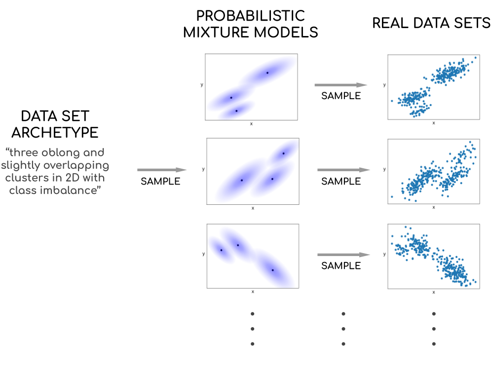
Figure 1: Illustration of synthetic data generation with data set archetypes. Left: the user specifies the desired archetype. Actual input is numeric but semantically similar to the natural language input shown. Middle: the archetype provides a random sampler for probabilistic mixture models with the desired geometric characteristics. Right: drawing i.i.d. samples from each mixture model yields synthetic data sets.

Generating synthetic data using geometric archetypes has several advantages. First, benchmarks of new algorithms will become more reliable. When a researcher creates synthetic data sets by hand to test a new algorithm, generating each new data set takes substantial effort. Thus, it is tempting to leave the data unchanged while tweaking the algorithm, which incurs an optimistic bias in the test results. Our data generator removes the incentive for tolerating this bias because it makes generating new synthetic data effortless.

Second, using data set archetypes makes benchmarks more reproducible. When researchers use one-off methods to generate synthetic data, each benchmark is unique and cannot be directly compared to another benchmark. By contrast, imagine testing a new algorithm on 1,000 synthetic data sets drawn from archetype $\mathcal{A}$. In this case, another researcher can immediately replicate the benchmark by drawing new data from archetype $\mathcal{A}$. Both researchers’ data sets will have the same underlying probability distribution. The same benefit applies to more sophisticated benchmarks using a collection $\{\mathcal{A}_{1},\mathcal{A}_{2},...,\mathcal{A}_{n}\}$ of archetypes.

Third, using data set archetypes makes benchmarks more interpretable. Since each archetype has an intuitive meaning, breaking down benchmark results by archetype makes it easier to evaluate the strengths and weaknesses of an algorithm. We give such a breakdown in Section 7.

Figure 2 visualizes repliclust’s ability to generate similar but distinct data sets. In the figure, each column depicts data sets generated from a different archetype.

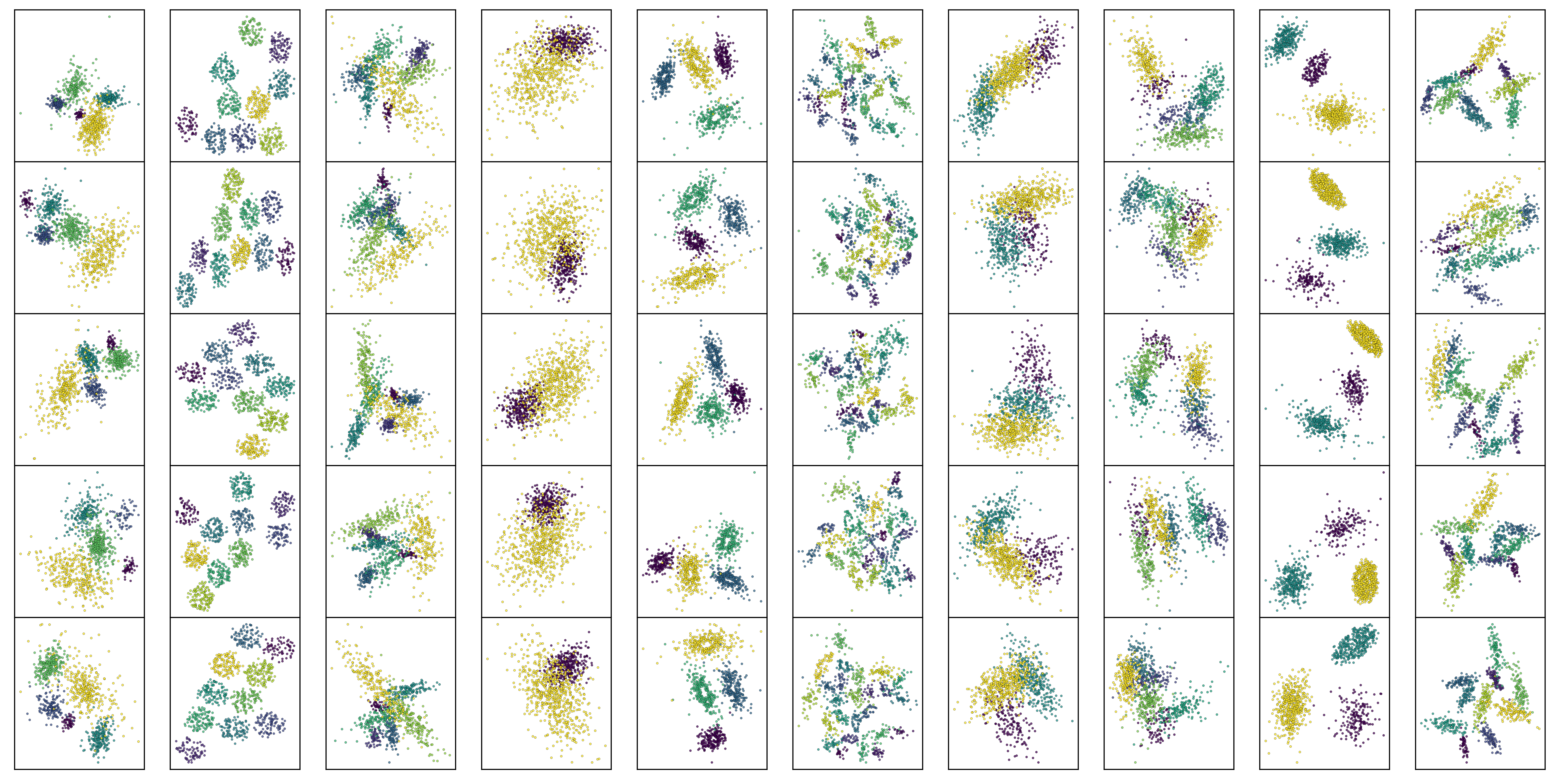
Figure 2: Synthetic data sets generated from different archetypes. Each column of scatter plots shows data sets sampled i.i.d. from the same archetype. Within each scatter plot, the coloring indicates different clusters.

In the next section, we explain the definitions of clusters and mixture models in repliclust.

3 Representing Clusters and Mixture Models

We now discuss repliclust’s internal model for clusters and probabilistic mixture models. The parameters we describe in this section, such as cluster axes, do not constitute user input. Instead, they are sampled automatically via data set archetypes. Nevertheless, these parameters play an important role because they determine the complexity of the data we can generate.

3.1 Clusters

In repliclust, we generate ellipsoidal clusters with diverse probability distributions by sampling radially using a univariate base distribution. For example, suppose the base distribution is an exponentially distributed random variable $Z$. We construct an ellipsoidal distribution in $p$ dimensions by first sampling the radius $R=\sqrt{\sum_{i=1}^{p}Z_{i}^{2}}$ of a random vector $(Z_{1},Z_{2},...,Z_{p})$ with i.i.d. entries, then selecting a unit vector $\hat{\boldsymbol{r}}$ uniformly at random. The product $R\hat{\boldsymbol{r}}$ defines an isotropic (spherical) multivariate distribution, which we transform to an ellipsoidal shape by left-multiplying with the square root $\boldsymbol{\Sigma}^{\frac{1}{2}}$ of a cluster-specific covariance matrix $\boldsymbol{\Sigma}$. The random vector $\boldsymbol{\Sigma}^{\frac{1}{2}}R\hat{\boldsymbol{r}}$ defines the distribution of a cluster’s spread around its center.

To make the overall spread of a cluster depend only on its covariance matrix, rather than its base distribution, we peg the $68.2\%$ quantile of the absolute value of each base distribution at unity. For example, if the base random variable $Z$ is exponential with rate $\lambda$, we would actually use the rescaled variable $Z/q_{0.682}$, where the quantile $q_{0.682}$ satisfies $\mathbb{P}(|Z|\leq q_{0.682})=0.682$. This rescaling puts all distributions on the same scale as the multivariate normal distribution, which natively satisfies $\mathbb{P}(|\mathcal{N}(0,1)|\leq 1)\approx 0.682$.

As a result of normalizing each base distribution, the overall shape of a cluster depends only on its center and covariance matrix. The covariance matrix decomposes into a set of orthonormal eigenvectors $\hat{\boldsymbol{u}}_{1},\hat{\boldsymbol{u}}_{2},...,\hat{\boldsymbol{u}}_{p}$ and corresponding variances $\sigma_{1}^{2},\sigma_{1}^{2},...,\sigma_{p}^{2}$. We call the vectors $\sigma_{1}\hat{\boldsymbol{u}}_{1},\sigma_{2}\hat{\boldsymbol{u}}_{2},...,\sigma_{p}\hat{\boldsymbol{u}}_{p}$ the principal axes of a cluster. These axes determine whether a cluster is long and thin, or short and stout, and in which direction it points. For a normally distributed cluster, the length of each principal axis is the marginal standard deviation along its direction.

Clusters with non-normal base distributions can provide useful insights into the robustness of a cluster analysis algorithm. At this time, repliclust explicitly support the beta, chi-square, exponential, F, gamma, Gumbel, lognormal, normal, Pareto, Student’s t, and Weibull distributions. In addition, it is possible to use any other distribution in Python’s numpy package.

Figure 3 visualizes clusters with different base distributions, highlighting the effects of heavy tails or bounded support. The upper three panels show distributions with successively heavier tails, resulting in a higher number of data points far away from the cluster center. By contrast, the second and third panels in the bottom row demonstrate that base distributions with holes (supported away from zero) lead to clusters with holes.

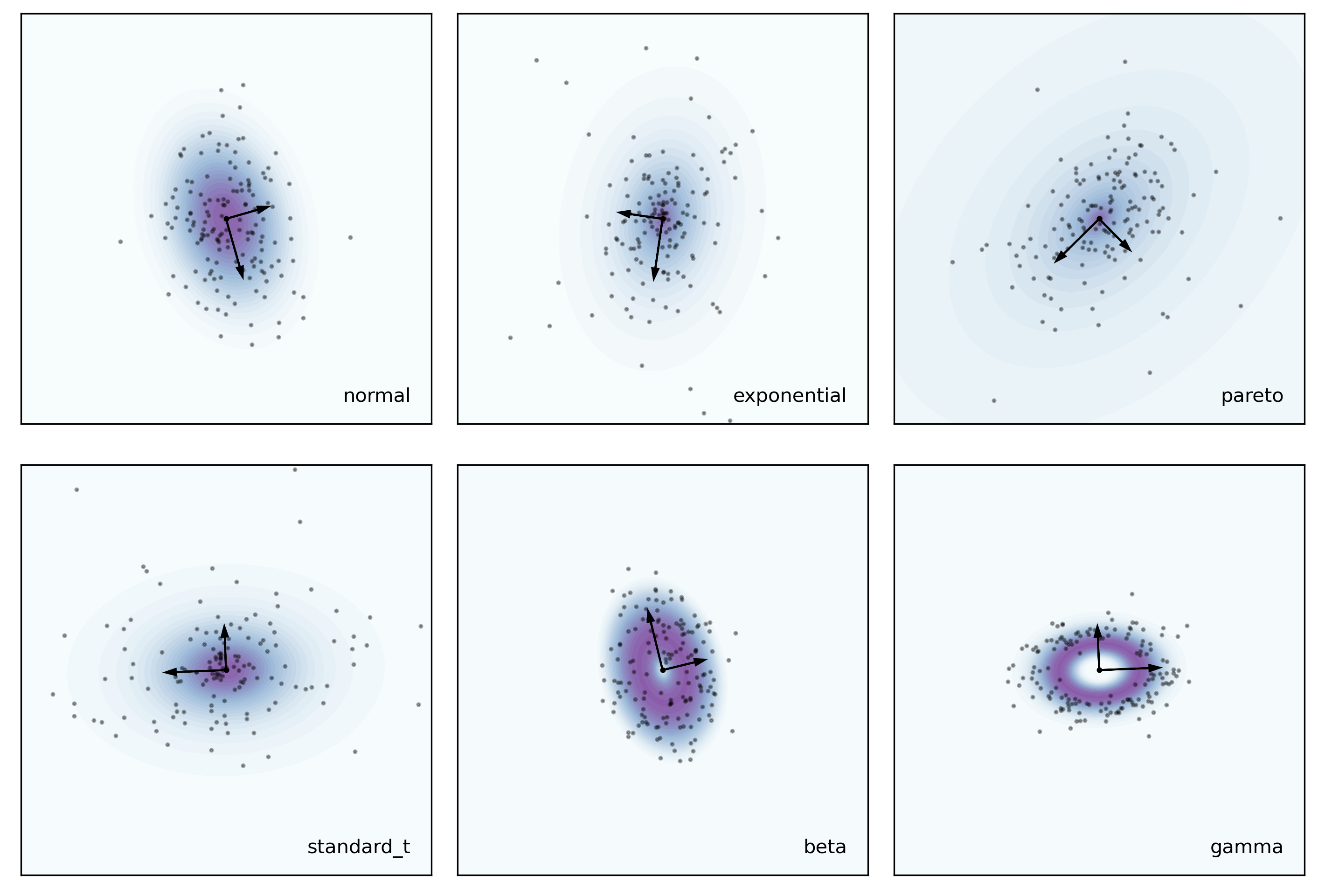
Figure 3: Clusters based on different univariate probability distributions. Each cluster’s main geometric features are drawn in black: the central black dot is the cluster center; the arrows emanating from it are the principal axes. The gray dots are data points sampled according to the cluster distribution. The shape parameters are a=3 for pareto; df=3 for standard_t; a=2, b=3 for beta; and shape=10 for gamma.

3.2 Probabilistic Mixture Models

Probabilistic mixture models in repliclust are blueprints for individual synthetic data sets. The MixtureModel object encodes the location, shape, and probability distribution of each cluster in a data set. Different clusters are oriented at arbitrary angles with respect to each other, and their shapes can vary from perfectly spherical to strongly ellipsoidal, all in the same data set. Figure 4 visualizes a probabilistic mixture model and plots a data set sampled from it.

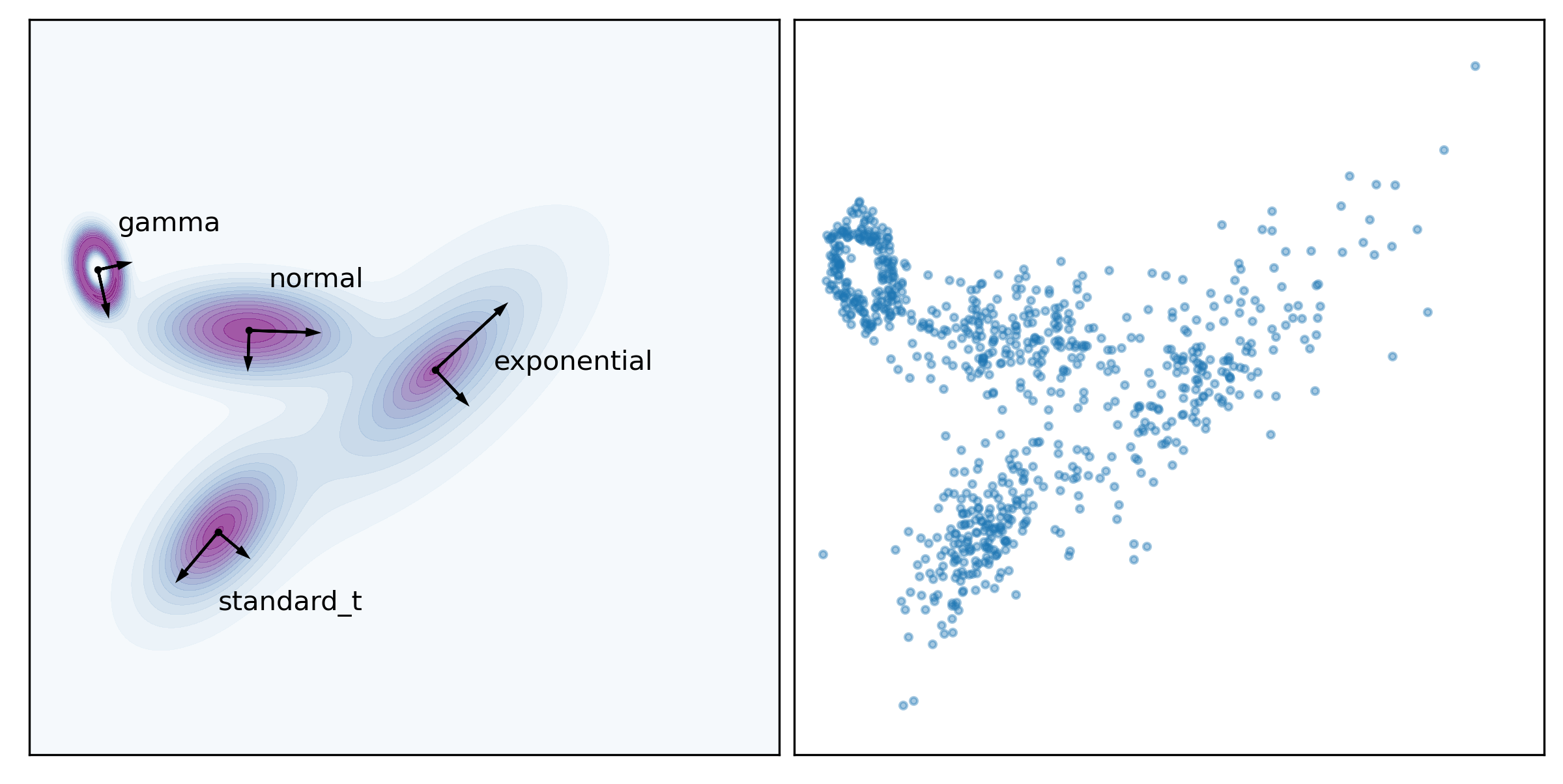
Figure 4: A probabilistic mixture model in repliclust. Left: visualization of the mixture model. Each cluster has its own shape, orientation, and probability distribution. The principal axes of each cluster are drawn as black arrows. The labels name each cluster’s univariate base probability distribution. The shape parameters for the distributions are shape=10 for gamma and df=5 for standard_t. Right: a data set sampled from the mixture model on the left ($n=800$ data points).

Table 1 lists the formal attributes of a mixture model. Each data set archetype defines a probability distribution over these attributes, providing a way to randomly sample similar mixture models.

Table 1: Internal representation of a mixture model.

Attribute Meaning Mathematical Definition cluster centers the positions of cluster centers in space $\boldsymbol{\mu}_{1},\boldsymbol{\mu}_{2},...,\boldsymbol{\mu}_{k}\in\mathbb{R}^{p}$ principal axis orientations the spatial orientation of each cluster’s ellipsoidal shape (different for each cluster) orthonormal matrices $\mathbf{U}_{1},\mathbf{U}_{2},...,\mathbf{U}_{k}\in\mathbb{R}^{p\times p}$ principal axis lengths the lengths of each cluster’s principal axes (axes have different lengths between and within clusters) $\boldsymbol{\sigma}_{1},\boldsymbol{\sigma}_{2},...,\boldsymbol{\sigma}_{k}\in{(\mathbb{R}^{>0}})^{p}$ cluster distributions multivariate probability distributions for generating data (different for each cluster) distributions $\mathbb{P}_{1},\mathbb{P}_{2},...,\mathbb{P}_{k}$

4 Specifying a Data Set Archetype

In this section, we explain how to specify a data set archetype in repliclust. Recall that an archetype defines a probability distribution over mixture models, allowing the user to generate similar but distinct synthetic data sets.

The user specifies an Archetype object by selecting high-level parameters determining geometric attributes such as 1) the number of clusters and dimensionality of the data, 2) the typical shape of a cluster and its expected variation within a data set, 3) the degree of overlap between clusters, 4) the imbalance in the number of data points per cluster, and 5) the possible probability distributions for each cluster. There are different ways to parameterize such attributes. Table 2 summarizes our default implementation. In practice, it is not necessary to provide an input for every parameter since repliclust provides sensible default values.

Table 2: Summary of user-specified parameters for defining an Archetype in repliclust.

Parameter(s) Purpose n_clusters / dim / n_samples select number of clusters / dimensions / data points aspect_ref / aspect_maxmin determine how elongated vs spherical clusters are / how much this varies between clusters radius_maxmin determine the variation in cluster volumes max_overlap / min_overlap set maximum / minimum overlaps between clusters imbalance_ratio make some clusters have more data points than others distributions / distribution_proportions select probability distributions appearing in each data set / how many clusters have each distribution

Many of the parameters listed in Table 2 are based on what we call “max-min sampling.” In this approach, the user controls a geometric attribute by specifying a reference value and max-min ratio. For example, the aspect ratio of a cluster measures how elongated it is. On the one hand, it is a max-min ratio in its own right, since it equals the ratio of the lengths of the longest cluster axis to the shortest. On the other hand, it is also subject to control through max-min sampling. The parameter aspect_ref sets the typical aspect ratio among all clusters in a data set, while aspect_maxmin sets the ratio of the highest to the lowest aspect ratio. Max-min sampling allows us to generate an aspect ratio $\alpha_{j}$ for each cluster in a data set ($j=1,2,3,...,k$), subject to the location and scale constraints $(\prod_{j=1}^{k}\alpha_{j})^{\frac{1}{k}}=\texttt{aspect\_ref}$ and $\frac{\max_{j\in\{1,...,k\}}\alpha_{j}-1}{\min_{j\in\{1,...,k\}}\alpha_{j}-1}=\texttt{aspect\_maxmin}$. In Appendix A, we give more details on how we manage different geometric attributes using max-min parameters.

In contrast to cluster shapes, the orientation of each cluster is not subject to user control. For each cluster, we sample the directions of its principal axes using the uniform distribution on orthogonal matrices, the so-called Haar measure (see Mezzadri (2007)).

The probability distribution of each cluster depends on univariate base distributions, as described in Section 3.1. Specifically, the distributions and distribution_proportions parameters of an Archetype specify the desired base distributions and their proportions among clusters. For example, if the user requests $30\%$ of clusters to be normally distributed, and the remaining $70\%$ to be exponentially distributed, then we randomly assign normal distributions to $30\%$ of clusters in each data set.

The last important attribute of an Archetype is overlap control. To specify the overlap between clusters, the user selects the max_overlap and min_overlap parameters. These values are percentages. For example, $\texttt{max\_overlap}=0.05$ indicates at most $5\%$ overlap between clusters. In the next section, we discuss overlap control in more detail.

5 Managing Cluster Overlaps

Managing the degree of overlaps between clusters is one of the most important tasks of a cluster generator. For example, in benchmarks of clustering algorithms, synthetic data sets with significant overlap between clusters make it possible to test a new algorithm on challenging data sets. In repliclust, we define overlap between two clusters in terms of the irreducible error rate when classifying a new data point as belonging to one of the clusters.

This framework recalls the quantile-based separation index introduced by Qiu and Joe (2006b). It requires thinking of clusters as multivariate probability distributions. This approach seems reasonable since many clustering algorithms implicitly define probabilistic models. For example, the popular K-Means algorithm is equivalent to maximizing the likelihood of classifying each data point as a sample from one of $k$ distinct multivariate normal distributions (with a priori unknown means). Thus, measuring cluster overlap in terms of irreducible classification error guarantees that, as cluster overlap increases, K-Means performs worse. This desirable relationship suggests that our definition of cluster overlap partly reflects the intrinsic difficulty of a clustering problem. We empirically verify this claim in Section 7.

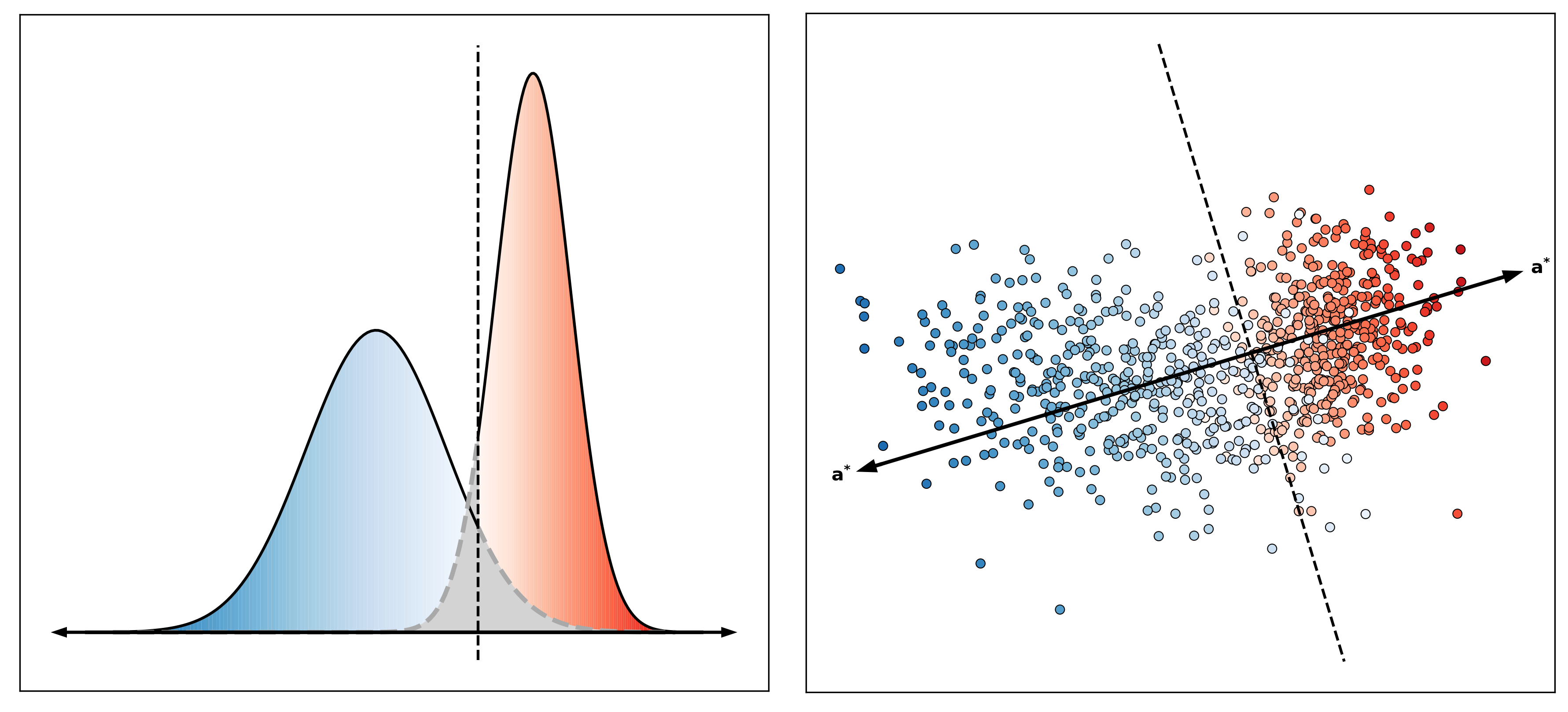
Figure 5: Cluster overlap based on the misclassification rate of the best linear classifier. The left panel shows the densities of two normal distributions colored by cumulative probability. Using a minimax decision rule, we classify an observation as having come from the blue or red distribution based on its location relative to the black dashed line. The gray shaded areas bounded by this line represent classification mistakes. When viewed as one-dimensional clusters, the distributions have overlap $\alpha=0.147$ (total gray area). The right panel shows two multivariate normal clusters in 2D. The black dashed line is the decision boundary based on the minimax classification axis $\boldsymbol{a}^{*}$. Data points from each cluster are colored according to cumulative probability along $\boldsymbol{a}^{*}$ and $-\boldsymbol{a}^{*}$, respectively. Cluster overlap is $\alpha=14.7\%$, implying that around $7.35\%$ of data points lie on the “wrong” side of the decision boundary, resulting in classification errors. The left panel shows the marginal distributions of the clusters in the right panel.

Formally, we define the overlap between two clusters as twice the minimax error rate when classifying new data points using a linear decision boundary between the two clusters. Figure 5 illustrates this definition. To explain what we mean by “minimax” in this context, observe that any linear classifier $\hat{y}:\mathbb{R}^{p}\mapsto\{1,2\}$ depends on an axis $\boldsymbol{a}\in\mathbb{R}^{p}$ and threshold $c\in\mathbb{R}$ such that

$$\hat{y}(\mathbf{x})=\begin{cases}1,&\text{if $\boldsymbol{a}^{\top}\mathbf{x}\leq c$}\\ 2,&\text{if $\boldsymbol{a}^{\top}\mathbf{x}>c$}.\end{cases}$$ (1)

By definition, the minimax classifier $\hat{y}^{*}$ minimizes the worst-case loss. In symbols,

$$\max_{y}~{}\mathbb{P}(y\neq\hat{y}^{*}(\mathbf{x})|y)=\min_{\hat{y}}\max_{y}~{}\mathbb{P}(y\neq\hat{y}(\mathbf{x})|y),$$ (2)

where $y\in\{1,2\}$ is the true cluster label corresponding to a new data point $\mathbf{x}\in\mathbb{R}^{p}$. The outer minimum on the right hand side ranges over all linear classifiers $\hat{y}$, including $\hat{y}^{*}$. Rewriting (2) in terms of the classification axes $\boldsymbol{a}$ and thresholds $c$ yields

$$\boldsymbol{a}^{*},~{}c^{*}=\operatorname*{arg\,min}_{\boldsymbol{a}\in\mathbb{R}^{p},~{}c\in\mathbb{R}}~{}\max\{~{}\mathbb{P}(\boldsymbol{a}^{\top}\mathbf{x}>c~{}|~{}y=1),~{}\mathbb{P}(\boldsymbol{a}^{\top}\mathbf{x}\leq c~{}|~{}y=2)~{}\}.$$ (3)

It is not hard to see that the minimax condition requires the cluster-specific error rates $\mathbb{P}(\boldsymbol{a^{*}}^{\top}\mathbf{x}>c^{*}~{}|~{}y=1)$ and $\mathbb{P}(\boldsymbol{a^{*}}^{\top}\mathbf{x}\leq c^{*}~{}|~{}y=2)$ to be equal. Consequently, the cluster overlap $\alpha$ becomes

$$\alpha=2~{}\mathbb{P}(\boldsymbol{a^{*}}^{\top}\mathbf{x}>c^{*}~{}|~{}y=1).$$ (4)

Geometrically, our definition means that two clusters overlap at level $\alpha$ if their marginal distributions along the minimax classification axis $\boldsymbol{a}^{*}$ intersect at the $1-\alpha/2$ and $\alpha/2$ quantiles. The left panel of Figure 5 highlights the probability mass bounded by these quantiles in gray.

Next, we turn to computing the cluster overlap $\alpha$. Conceptually, any difficulty in solving (3) lies in finding the classification axis $\boldsymbol{a}^{*}$. By contrast, it is easy to compute the threshold $c$ from the equality of the cluster-specific misclassification rates. Anderson and Bahadur (1962) describe an algorithm for computing $\boldsymbol{a}^{*}$ exactly, in the case of multivariate normal distributions. Their method requires finding the zero of a function $f(t)$ monotonic in $t\in[0,1]$. Each evaluation of $f(t)$ requires computing the matrix inverse $(t\boldsymbol{\Sigma}_{1}+(1-t)\boldsymbol{\Sigma}_{2})^{-1}$, where $\boldsymbol{\Sigma}_{1},\boldsymbol{\Sigma}_{2}$ are the clusters’ covariance matrices.

In practice, computing cluster overlap exactly may not be necessary. In the following, we suggest two approximations based on replacing the minimax classification axis $\boldsymbol{a}^{*}$ with a reasonable substitute.

First, it is possible to use a decision boundary based on linear discriminant analysis (LDA). For a pair of multivariate normal clusters with means $\boldsymbol{\mu}_{1}\neq\boldsymbol{\mu}_{2}$ and the same covariance matrix $\boldsymbol{\Sigma}$, the axis $\boldsymbol{a}_{\text{\tiny{LDA}}}=\boldsymbol{\Sigma}^{-1}(\boldsymbol{\mu}_{2}-\boldsymbol{\mu}_{1})$ minimizes the misclassification rate (see Hastie et al. (2009)). Unfortunately, this is not the case for unequal covariance matrices $\boldsymbol{\Sigma}_{1}\neq\boldsymbol{\Sigma}_{2}$. In this case, the choice $\boldsymbol{a}_{\text{\tiny{LDA}}}=(\frac{\boldsymbol{\Sigma}_{1}+\boldsymbol{\Sigma}_{2}}{2})^{-1}(\boldsymbol{\mu}_{2}-\boldsymbol{\mu}_{1})$ yields a good approximation. The following result shows how to compute the approximate cluster overlap based on $\boldsymbol{a}_{\text{\tiny{LDA}}}$.

Theorem 1 (LDA-Based Cluster Overlap)

For two multivariate normal clusters with means $\boldsymbol{\mu}_{1}\neq\boldsymbol{\mu}_{2}$ and covariance matrices $\boldsymbol{\Sigma}_{1},\boldsymbol{\Sigma}_{2}$, the approximate cluster overlap $\alpha_{\text{\tiny{LDA}}}$ based on the linear separator $\boldsymbol{a}_{\text{\tiny{LDA}}}=(\frac{\boldsymbol{\Sigma}_{1}+\boldsymbol{\Sigma}_{2}}{2})^{-1}(\boldsymbol{\mu}_{2}-\boldsymbol{\mu}_{1})$ is

$$\alpha_{\text{\tiny{LDA}}}=2\big{(}1-\Phi\Big{(}\frac{\boldsymbol{a}_{\text{\tiny{LDA}}}^{\top}(\boldsymbol{\mu}_{2}-\boldsymbol{\mu}_{1})}{\sqrt{\boldsymbol{a}_{\text{\tiny{LDA}}}^{\top}\boldsymbol{\Sigma}_{1}\boldsymbol{a}_{\text{\tiny{LDA}}}}+\sqrt{\boldsymbol{a}_{\text{\tiny{LDA}}}^{\top}\boldsymbol{\Sigma}_{2}\boldsymbol{a}_{\text{\tiny{LDA}}}}}\Big{)}\big{)},$$ (5)

where $\Phi(z)$ is the cumulative distribution function of the standard normal distribution. Moreover, if $\boldsymbol{\Sigma}_{1}=\lambda\boldsymbol{\Sigma}_{2}$ for some $\lambda$ then $\alpha_{\text{\tiny{LDA}}}$ equals the exact cluster overlap $\alpha$.

We prove this result in Appendix B. The main weakness of Theorem 1, from the perspective of a synthetic data generator, is the inversion of the matrix $\frac{\boldsymbol{\Sigma}_{1}+\boldsymbol{\Sigma}_{2}}{2}$. For $k$ cluster centers in $p$ dimensions, computing this inverse for each pair takes $O(k^{2}p^{3})$ operations. Fortunately, the speed of contemporary numerical linear algebra packages makes this computational cost affordable for many use cases, for instance in the range $p\leq 1000$.

To compute cluster overlap faster, at the cost of greater imprecision, it possible to separate two clusters using the line connecting their centers. The following result shows how to compute this second approximation.

Theorem 2 (Center-to-Center Cluster Overlap)

For two multivariate normal clusters with means $\boldsymbol{\mu}_{1}\neq\boldsymbol{\mu}_{2}$ and covariance matrices $\boldsymbol{\Sigma}_{1},\boldsymbol{\Sigma}_{2}$, the center-to-center cluster overlap $\alpha_{\text{\tiny{C2C}}}$, which is defined as the overlap based on a classification boundary perpendicular to the line connecting the cluster centers, is

$$\alpha_{\text{\tiny{C2C}}}=2\big{(}1-\Phi\Big{(}\frac{\boldsymbol{\delta}^{\top}\boldsymbol{\delta}}{\sqrt{\boldsymbol{\delta}^{\top}\boldsymbol{\Sigma}_{1}\boldsymbol{\delta}}+\sqrt{\boldsymbol{\delta}^{\top}\boldsymbol{\Sigma}_{2}\boldsymbol{\delta}}}\Big{)}\big{)},$$ (6)

where $\boldsymbol{\delta}:=\boldsymbol{\mu}_{2}-\boldsymbol{\mu}_{1}$ is the vector difference between cluster centers and $\Phi(z)$ is the cumulative distribution function of the standard normal distribution.

Moreover, if the covariance matrices $\boldsymbol{\Sigma}_{1}$ and $\boldsymbol{\Sigma}_{2}$ are both multiples of the identity matrix, then $\alpha_{\text{\tiny{C2C}}}$ equals the exact cluster overlap $\alpha$.

We prove this result in Appendix B.

Given that we have approximated cluster overlap in two different ways, trading off speed and accuracy requires knowledge of the relative quality of these approximations. Figure 6 compares both approximations with the exact overlap (computed with the method suggested by Anderson and Bahadur (1962)). The results show that LDA-based overlap is significantly more accurate than center-to-center overlap. Nevertheless, both estimates are highly correlated with exact overlap.

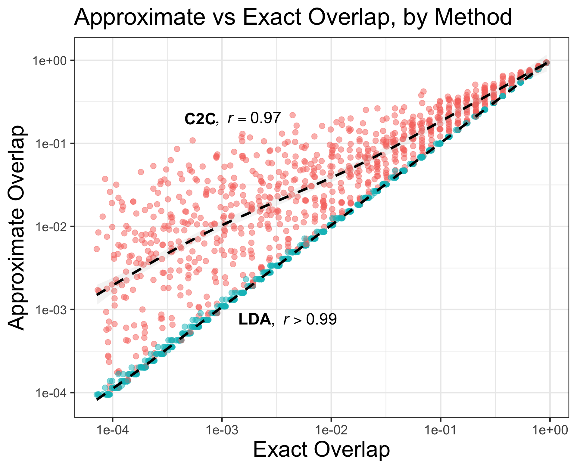
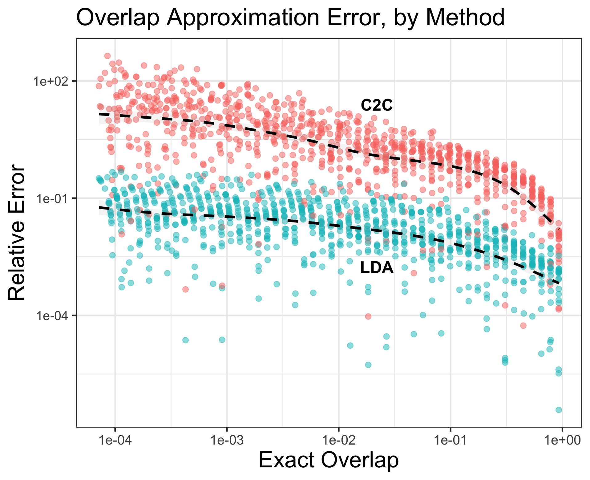
Figure 6: Quality of approximating cluster overlap using the LDA-based and center-to-center (C2C) methods. Each data point corresponds to a pair of multivariate normal clusters with the pairwise overlap shown. The full simulation is based on 900 pairs generated from a variety of data set archetypes with different cluster shapes and numbers of dimensions. The dashed lines estimate the conditional means. The C2C and LDA approximations are both highly correlated with exact cluster overlap, with Pearson correlations $r$ close to 1 (left). However, the C2C method incurs significant relative error, while the LDA approximation typically comes within 10% of the exact overlap (right).

Theorems 1-2 show that cluster overlap depends on quantiles $q$ of the form

$$q(\boldsymbol{\mu}_{1},\boldsymbol{\mu}_{2};\boldsymbol{\Sigma}_{1},\boldsymbol{\Sigma}_{2};\boldsymbol{a}) =\frac{\boldsymbol{a}^{\top}(\boldsymbol{\mu}_{2}-\boldsymbol{\mu}_{1})}{\sqrt{\boldsymbol{a}^{\top}\boldsymbol{\Sigma}_{1}\boldsymbol{a}}+\sqrt{\boldsymbol{a}^{\top}\boldsymbol{\Sigma}_{2}\boldsymbol{a}}},$$ (7)

where $\boldsymbol{a}$ is a classification axis. Since these quantiles are inversely related to cluster overlap, they quantify cluster separation. Carrying out computations in terms of the separation variables $q$ rather than the overlap variables $\alpha$ can enhance numerical stability.

Up until this point, our discussion centered on multivariate normal clusters. Indeed, repliclust uses the formulas derived from normal distributions to quantify overlaps between non-normal clusters. Since we rescale each non-normal base distribution such that its absolute value has a $68.15\%$ quantile of unity (as is true for the normal distribution), we expect adequate performance for non-normal clusters. Figure 7 shows synthetic data generated from data set archetypes with the same overlap but different probability distributions. The figure suggests adequate overlap control for non-normal clusters. In the next section, we discuss how repliclust quantifies overlap on whole data sets with $k>2$ clusters.

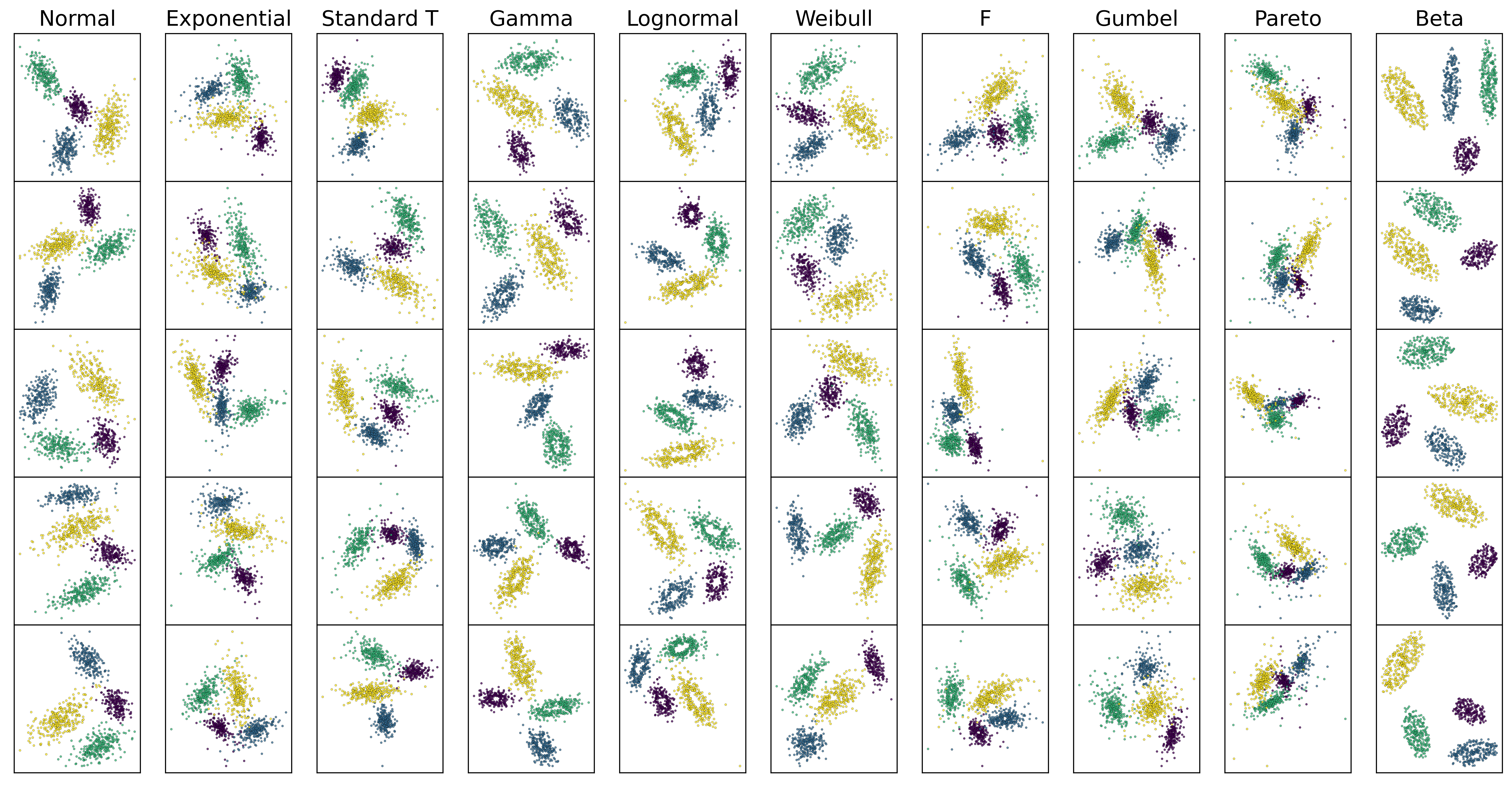
Figure 7: Overlap control with non-normal probability distributions. The data sets shown are generated from the same archetype (with overlap at around 1%), except that we change the probability distribution in each column. For each scatter plot, the coloring indicates different clusters. Note that using heavy-tailed distributions (Pareto, F, …) may lead to outliers, which makes clusters appear smaller on the scatter plots: this does not indicate greater overlap per se. The only distribution that seems to violate $1\%$ overlap is the beta distribution in the last column; this is a special case because the beta distribution only has probability mass on the finite interval $[0,1]$. Overall, our overlap metric derived from multivariate normal clusters appears to perform adequately even for non-normal clusters. All distributional parameters are given in Appendix C.

5.1 Constraining Overlaps of Multiple Clusters

Equations (5) and (6) allow us to compute the level of overlap between any pair of clusters. However, for a data set with $k$ clusters, it would be impractical to have the user select desired overlaps for all $k(k-1)/2$ pairs of clusters. To solve this problem, repliclust introduces two parameters: max_overlap imposes an upper bound on the level of overlap between any pair of clusters in the data set, thereby ensuring that no two clusters are too close to each other. Conversely, min_overlap requires each cluster to overlap at level $\geq\texttt{min\_overlap}$ with at least one other cluster. This requirement prevents isolated clusters, i.e., individual clusters far away from all other clusters.

To quantify and enforce compliance with the user-specified overlap constraints, we define a loss function. Given cluster centers $\{\boldsymbol{\mu}_{i}\}_{i=1}^{k}$ and covariance matrices $\{\boldsymbol{\Sigma}_{i}\}_{i=1}^{k}$, the overlap loss is

$$\mathcal{L}\big{(}\{\boldsymbol{\mu}_{i}\},\{\boldsymbol{\Sigma}_{i}\}\big{)}=\frac{1}{k}\sum_{i=1}^{k}\ell_{i},$$ (8)

where the loss on the $i$-th cluster is

$$\ell_{i}=p_{\lambda}\big{(}(\min_{j\neq i}q_{ij}-q_{\text{max}})^{+}\big{)}+\sum_{j\neq i}p_{\lambda}\big{(}(q_{\text{min}}-q_{ij})^{+}\big{)}.$$ (9)

Here, $q_{\text{min}}$, $q_{\text{max}}$, and $q_{ij}$ measure cluster separation as expressed in Equation 7: $q_{\text{min}}$ is the minimum allowed separation (corresponding to overlap $\alpha=\texttt{max\_overlap}$); $q_{\text{max}}$ is the maximum allowed separation (corresponding to $\alpha=\texttt{min\_overlap}$); and $q_{ij}$ is the separation between the $i$-th and $j$-th clusters. The penalty function $p_{\lambda}$ is the polynomial $p_{\lambda}(x):=\lambda x+(1-\lambda)x^{2}$, where $\lambda$ is a tuning parameter. Finally, $x^{+}:=\max(x,0)$ is a filter that passes on only positive inputs (corresponding to a violation of user-specified constraints).

By design, the loss (9) vanishes when the cluster centers $\{\boldsymbol{\mu}_{i}\}_{i=1}^{k}$ and covariance matrices $\{\boldsymbol{\Sigma}_{i}\}_{i=1}^{k}$ satisfy user-specified overlap constraints. The first term penalizes violation of the minimum overlap condition. Indeed, if cluster $i$ is too far away from the other clusters, the separation $\min_{j\neq i}q_{ij}$ between cluster $i$ and its closest neighbor exceeds the maximum allowed separation $q_{\text{max}}$. A penalty of the excess $(\min_{j\neq i}q_{ij}-q_{\text{max}})^{+}$ yields the first term in (9). The second term measures violation of the maximum overlap condition. If the separation $q_{ij}$ between clusters $i$ and $j$ falls short of the smallest allowed separation $q_{\text{min}}$, the shortfall $(q_{\text{min}}-q_{ij})^{+}$ incurs a penalty that serves to push these clusters apart.

The penalty $p_{\lambda}$ in (9) ranges from quadratic to linear based on the value of $\lambda$. Keeping the penalty partly linear ($\lambda>0$) helps gradient descent drive the overlap loss to exactly zero because a purely quadratic loss would result in a vanishing derivative when overlap constraints approach satisfaction.

5.2 Minimizing the Overlap Loss

Generating synthetic data in repliclust involves first sampling cluster shapes and then finding cluster centers for which the overlap loss vanishes. To find such cluster centers, we minimize (8) using stochastic gradient descent.

To initialize the minimization, we place cluster centers randomly within a sphere. The volume $V$ of this sphere influences the initial overlaps between clusters. To select an appropriate value, we fix the ratio $\rho$ of the sum of cluster volumes to $V$; essentially, $\rho$ is the density of clusters within the sampling volume. Values of $\rho$ around 10% work well in low dimensions. In higher dimensions, however, results from the mathematics of sphere-packing motivate a downward adjustment. A lower bound by Ball (1992) states that the maximum achievable density when placing non-overlapping spheres inside $\mathbb{R}^{p}$ is at least $p2^{1-p}$. Thus, in $p$ dimensions we use an adjusted density $\rho^{\text{adj}}$ defined by

$$\rho^{\text{adj}}(p)=p2^{1-p}\rho^{2D},$$

where $\rho^{2D}\approx 10\%$ is the equivalent density in 2D.

Following initialization, we optimize the cluster centers $\{\boldsymbol{\mu}_{i}\}_{i=1}^{k}$ using stochastic gradient descent. During this process, the covariance matrices $\{\boldsymbol{\Sigma}_{i}\}_{i=1}^{k}$ are fixed. Each iteration performs the update

$$\big{[}\boldsymbol{\mu}_{1}|\boldsymbol{\mu}_{2}|~{}...~{}|\boldsymbol{\mu}_{k}\big{]}~{}\leftarrow~{}\big{[}\boldsymbol{\mu}_{1}|\boldsymbol{\mu}_{2}|~{}...~{}|\boldsymbol{\mu}_{k}\big{]}~{}-~{}\eta~{}\big{[}\nabla_{\boldsymbol{\mu}_{1}}\ell_{i}|\nabla_{\boldsymbol{\mu}_{2}}\ell_{i}|~{}...~{}|\nabla_{\boldsymbol{\mu}_{k}}\ell_{i}\big{]}$$ (10)

on the single-cluster loss $\ell_{i}$, where $\eta$ is the learning rate. For each epoch, we randomly permute the order $i=1,2,...,k$ of clusters and apply the updates (10) in turn for each cluster.

Experiments suggest that our minimization procedure drives the overlap loss to zero at an exponential rate (linear convergence rate), as expected for gradient descent. The number of epochs required seems largely independent of the number of clusters, though it increases slightly with the number of dimensions.

In the next section, we discuss the modular software architecture of repliclust.

6 Modular Software Architecture

The Python code underlying repliclust uses object-oriented programming to promote usability and extensibility.

At the top of the object hierarchy, a DataGenerator produces ready-to-use synthetic data sets at the user’s command. The main input to a DataGenerator is one or more data set archetypes. An Archetype object coordinates the tasks involved in sampling similar but distinct probabilistic mixture models. These tasks are performed by specialized objects of type CovarianceSampler, ClusterCenterSampler, GroupSizeSampler and DistributionMix. These objects encode algorithms for sampling cluster shapes, centers, the number of data points in each cluster, and cluster probability distributions.

Figure 8: Object-oriented software architecture of repliclust. Each box represents an object. A solid arrow $A\leftarrow B$ means that $B$ is an attribute of $A$, while a dashed arrow $X\dashrightarrow Y$ means that $X$ randomly samples instances of $Y$. An Archetype samples mixture models, and each MixtureModel samples synthetic data sets. The DataGenerator acts a top-level wrapper for this workflow.

The repliclust code base defines all these objects in terms of flexible base classes. Concrete implementations require choices about how to map high-level geometric attributes to a small number of user-specified parameters (to define an Archetype), how to compute cluster overlap (to define a ClusterCenterSampler), how to parameterize class imbalance (to define a GroupSizeSampler), etc. Our default implementation represents one way of making these choices, expressed in the form of subclasses extending the implementation-agnostic base classes. For example, our default implementation for an Archetype is a subclass called MaxMinArchetype (named after the max-min parameters described in Section 4), which extends the Archetype base class.

This modular software architecture makes it easy to update parts of the workflow without affecting others. For example, to manage cluster overlaps differently, it suffices to write a new subclass extending the ClusterCenterSampler base class, while keeping in place the default implementations for the CovarianceSampler, GroupSizeSampler, and DistributionMix classes.

Figure 8 provides a diagram of our software architecture. A concise user guide is available at repliclust.org, allowing prospective users to start generating synthetic data within minutes. In the next section, we demonstrate the practical utility of repliclust.

7 Empirical Results

In this section, we provide empirical support for the utility of our software. First, we show that repliclust’s definition of cluster overlap reflects empirical clustering performance. Second, we run a small benchmark comparing the performance of the K-Means and Gaussian mixture algorithms for clustering. By including multiple data set archetypes in the benchmark, repliclust helps us understand how the algorithms’ performance varies with the overall characteristics of the data.

7.1 Relating Overlap to Clustering Performance

Figure 9 shows the results of a simulation study relating repliclust’s user-specified cluster overlap to the empirical performance of the K-Means algorithm. The figure shows the results of clustering a variety of synthetic data sets generated from different archetypes. Overall, we observe a strong negative correlation between cluster overlap and clustering performance. This relationship holds in 10, 100, and 500 dimensions, although performance suffers with increasing dimensionality. The number of clusters seems to play no role.

In this and subsequent figures, we report clustering performance using the adjusted mutual information (AMI). This metric measures the agreement between the inferred and ground truth cluster labels (see Vinh et al. (2009)). Higher values indicate greater agreement and better performance, with a value of 1 indicating a perfect match up to permutations.

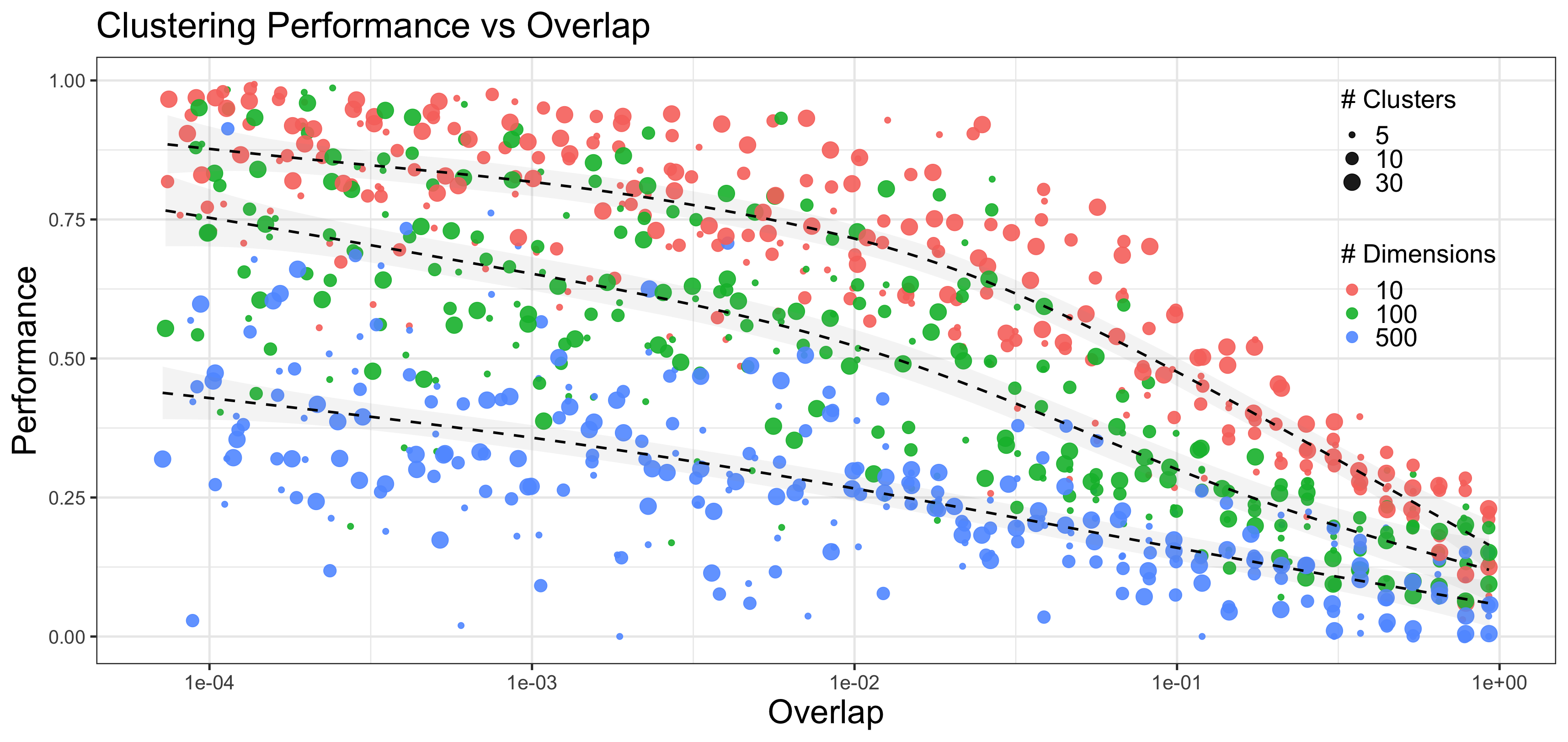
Figure 9: Inverse relationship between repliclust’s cluster overlap and the empirical performance of K-Means clustering. Performance is reported in terms of the adjusted mutual information, which measures the agreement between inferred and ground truth cluster labels, with a value of 1 indicating perfect agreement (up to permutations). The dots represent synthetic data sets generated from a diversity of randomly chosen data set archetypes. The dotted lines estimate the conditional mean of clustering performance given overlap, stratified by dimensionality of the data sets. The uncertainty bands show the standard error.

7.2 Comparing K-Means and Gaussian Mixtures

We now illustrate the power of repliclust by comparing the performance of two popular clustering algorithms: K-Means and Gaussian mixture models. Although our benchmark is small in scope, the point is that it was effortless to carry out. Setting up the benchmark in an interactive Python notebook took around 10-15 minutes.

Before presenting the results, we briefly review the two algorithms. K-Means minimizes the distances between data points and cluster centers, offering a simple yet reliable approach. On the other hand, a Gaussian mixture model (GMM) uses the expectation-maximization algorithm to fit cluster centers, covariance matrices, and class probabilities. In what follows, we only consider the “full” version of the GMM algorithm, which estimates a different covariance matrix for each cluster.

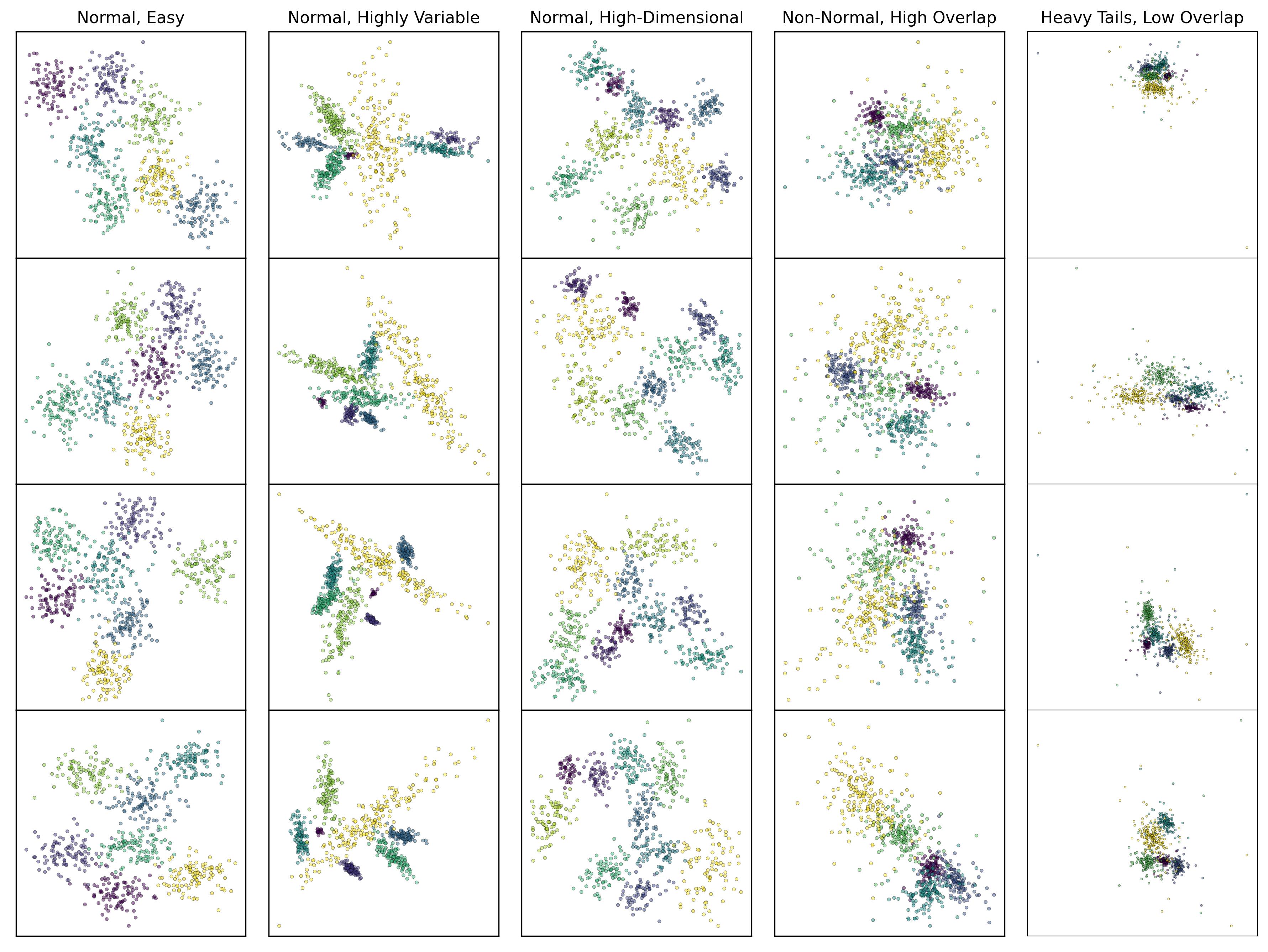
Figure 10: Illustration of data set archetypes used in the benchmark. Each column of scatter plots shows data sets sampled i.i.d. from the same different archetype, with the coloring indicating clusters. In the benchmark, we use higher-dimensional data sets (10- and 200-dimensional) generated from the same archetypes. Note that the heavy-tailed data sets appear to have greater overlap because the presence of outliers zooms out the view.

To set up the benchmark, we define a collection of data set archetypes: 1) “Normal, Easy”; 2) “Normal, Highly Variable”; 3) “Normal, High-Dimensional”; 4) “Non-Normal, High Overlap”; and 5) “Heavy Tails, Low Overlap.” In all cases, the word “normal” refers to normally distributed clusters. Figure 10 illustrates these archetypes in 2D. In the benchmark, however, all data sets are 10-dimensional except those generated from the “Normal, High-Dimensional” archetype, which are 200-dimensional. Full parameter settings can be found in Appendix C. For each archetype, we generate 300 data sets (adding to 1,500 data sets for the whole benchmark). We report clustering performance in terms of the adjusted mutual information (AMI), which measures the agreement between the inferred and ground truth cluster labels on a scale from 0 to 1, with a value of 1.0 indicating perfect agreement up to permutations of the cluster labels.

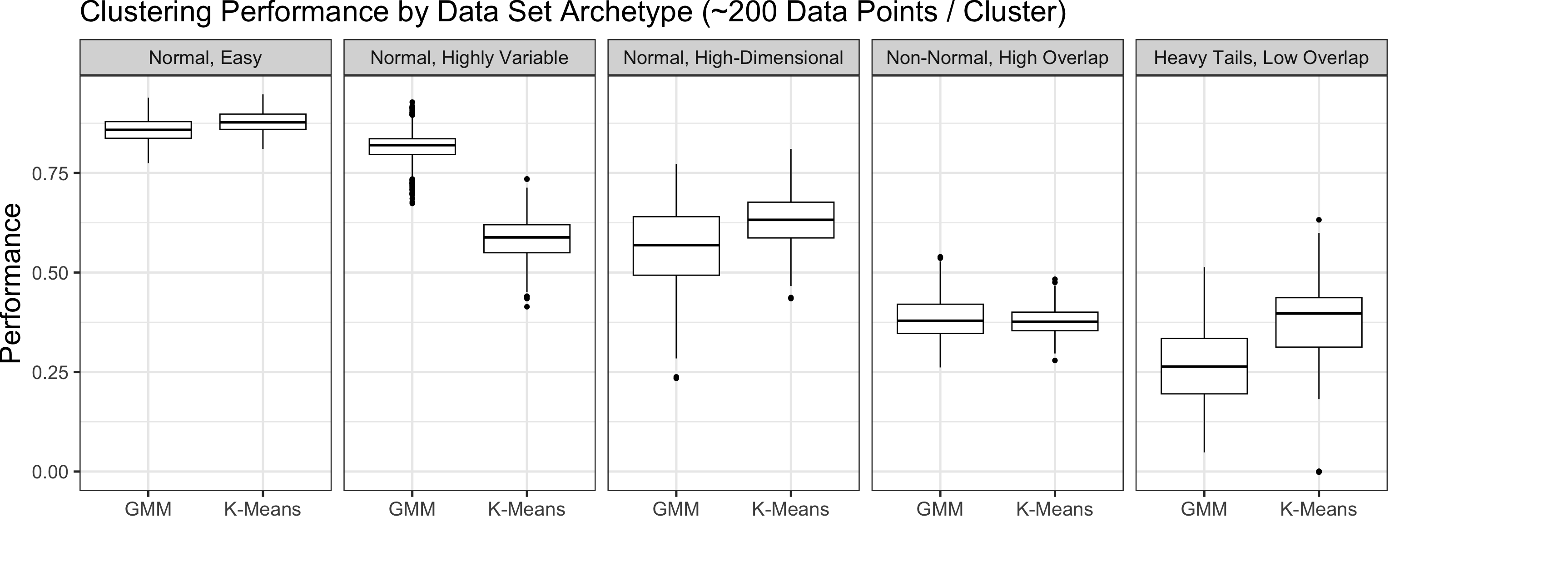
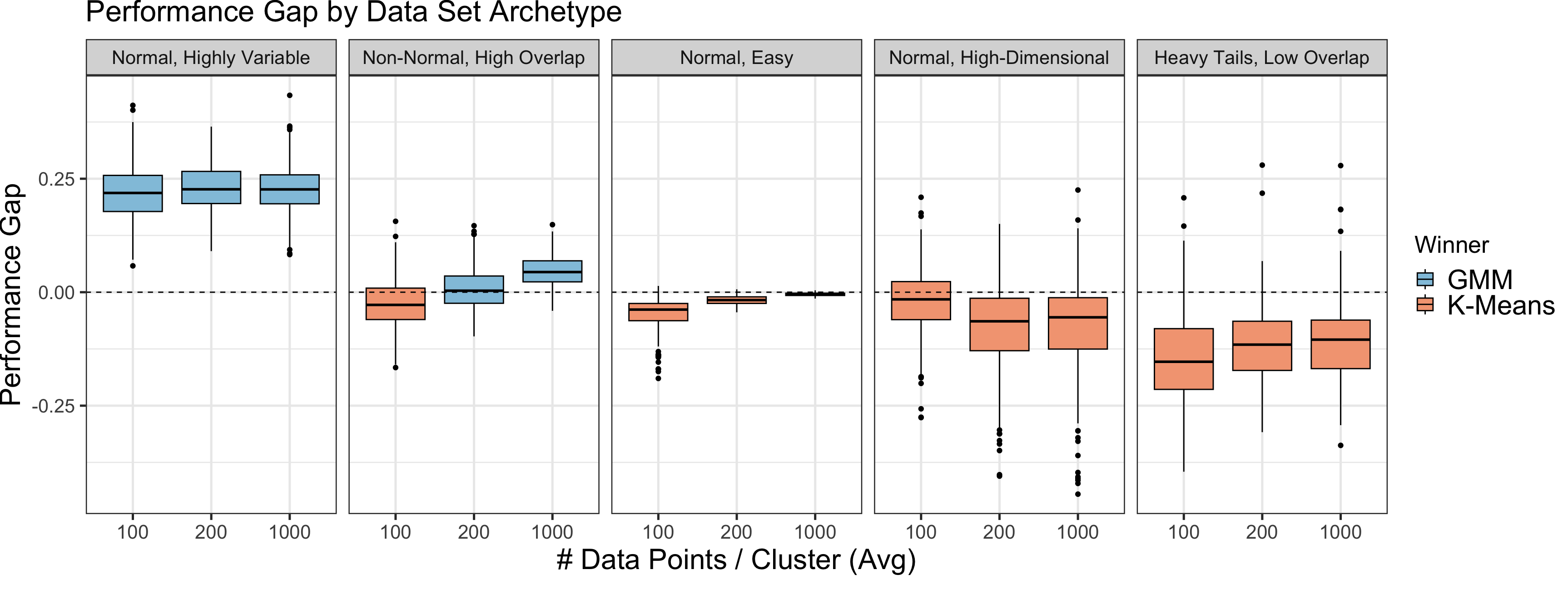
Figure 11: Clustering performance of K-Means and Gaussian Mixture models (GMM) on a variety of data set archetypes. The top panel shows absolute performance, whereas the bottom panel shows differences in performance between GMM and K-Means. Performance is measured using the adjusted mutual information (AMI), which quantifies the agreement between the inferred and ground truth cluster labels on a scale from 0 to 1. Higher values of the AMI indicate better performance, with a value of 1.0 indicating perfect agreement up to permutations. In the bottom panel, we call a winner when the performance gap exceeds the standard error of its mean. Each box plot is based on $n=300$ synthetic data sets generated i.i.d. from the respective archetype.

Figure 11 shows the results of the benchmark. The top panel shows the absolute performance of GMM and K-Means when sampling around 200 data points per cluster, whereas the lower panel shows the differences in performance for sample sizes of 100, 200, and 1000 data points per cluster (on average).

The results indicate that at any sample size, GMM performs much better on data sets with highly variable cluster shapes, as represented by the “Normal, Highly Variable” archetype. On the other hand, K-Means performs better on high-dimensional data (“Normal, High-Dimensional”) and clusters with heavy-tailed distributions (“Heavy Tails, Low Overlap”). The weakness of GMM on high-dimensional data is understandable since the method fits $O(p^{2}/2)$ parameters per cluster in $p$ dimensions, compared to $O(p)$ for K-Means.

On the remaining two data set archetypes, K-Means and GMM perform roughly equally well. On the “Non-Normal, High Overlap” archetype, which specifies exponentially distributed clusters with high overlap, the winner depends on the sample size. By contrast, the “Normal, Easy” archetype generates spherical multivariate normal clusters with equal variances. On this data, K-Means always leads but GMM closes the gap as the sample size increases.

The fact that GMM excels at highly variable cluster shapes, while K-Means tolerates heavy-tailed distributions better, poses an interesting question. Which method would perform better on a data set archetype that combines highly variable cluster shapes and heavy-tailed distributions? To find out, we ran an additional benchmark on a collection of data set archetypes based on the “Normal, Highly Variable” archetype but with one key difference: the clusters have distributions with successively heavier tails. Using repliclust, it took only 5 minutes to define the additional archetypes and start the benchmark.

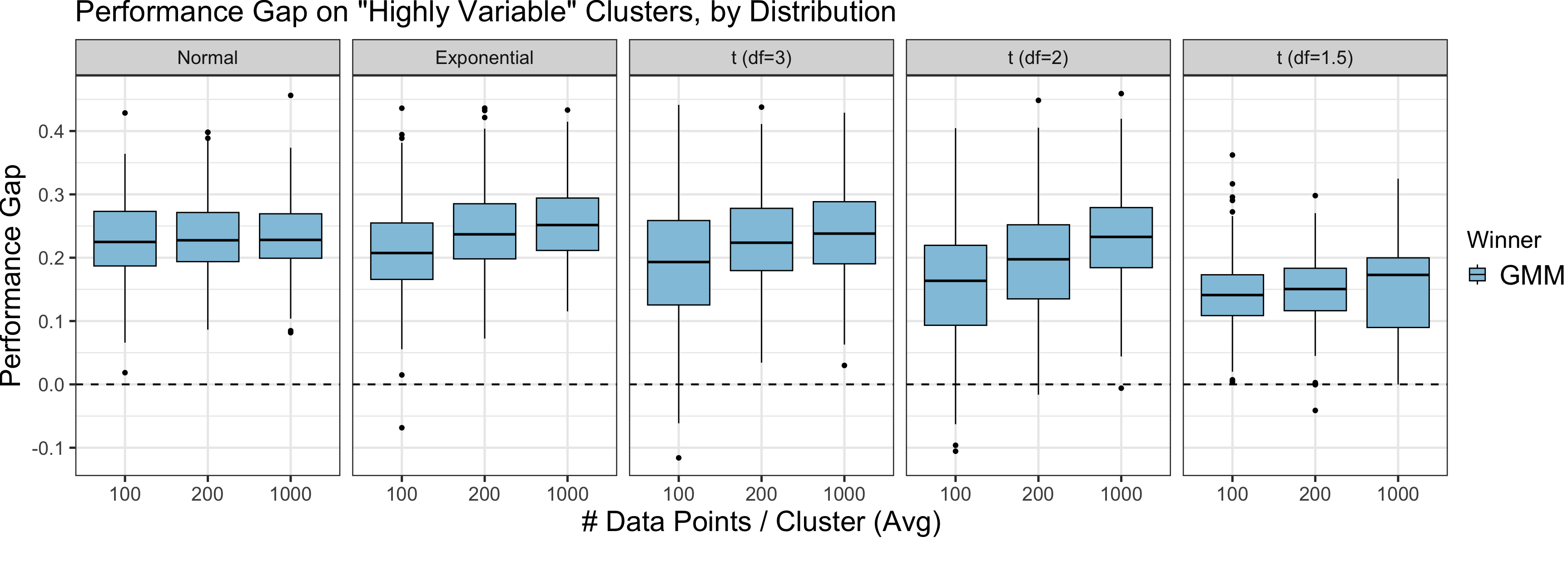
Figure 12: Performance gap between GMM and K-Means clustering on data sets with highly variable cluster shapes, for increasingly heavy-tailed distributions. The y axis shows the difference between the adjusted mutual information (AMI) for GMM and K-Means. The AMI measures the agreement between inferred and ground truth cluster labels on a scale of 0 to 1; higher numbers indicate better performance. Each box plot is based on $n=300$ synthetic data sets generated i.i.d. from the respective data set archetype.

Figure 12 displays the results. We observe that GMM maintains its advantage: it outperforms K-Means on data with highly variable cluster shapes, no matter whether the distribution is light- or heavy-tailed.

8 Discussion

This paper presents repliclust, a synthetic data generator for cluster analysis. Our main contribution is to introduce data set archetypes. To implement this idea, we introduced several practical innovations. For example, we use max-min parameters to define the overall geometric characteristics of a data set with clusters. In addition, we define cluster overlap based on minimax classification error (along with useful approximations) and encode this definition in a loss function. Finally, repliclust uses a flexible definition of probabilistic mixture models, giving the user more control over data geometry than comparable software.

Our interpretable benchmark in Section 7 highlights the advantages of synthetic data based on data set archetypes. Just like any other synthetic data, it is objective because the cluster identity of each data point is unambiguous, and manipulable because the user can change individual geometric attributes while leaving others constant. However, it is also fungible, in the sense that sampling from a data-generating probability distribution makes individual data sets freely replaceable. This last quality bestows the gift of nearly unlimited statistical power. In our benchmark between K-Means and Gaussian mixture models, we could sample as many i.i.d. data sets from each archetype as we wished, subject only to (moderate) computational limitations.

Acknowledgments

MJZ would like to acknowledge support from Matt Thomson and members of the Thomson Lab at Caltech. In addition, MJZ thanks Dante Roy Calapate for providing his computer monitor during the early stages of this project.

Appendix A

We give more detail on how repliclust manages various geometric attributes using max-min parameters. Table 3 lists all geometric attributes managed with max-min sampling and names the corresponding parameters in repliclust.

Table 3: Summary of geometric attributes managed with max-min sampling. The second and third columns indicate whether each max-min ratio or reference value is inferred, or specified by the user as a parameter. The fourth column gives the location constraint used during max-min sampling. The group size of a cluster is the number of data points in it; the aspect ratio is the ratio of the lengths of the longest cluster axis to the shortest. For cluster volumes, we specify the reference value and max-min ratio in terms of radius (dim-th root of volume) since volumes grow rapidly in high dimensions.

Geometric Parameter Max-Min Ratio Reference Value Constraint cluster volumes radius_maxmin scale cluster volumes average to reference volume group sizes imbalance_ratio average group size group sizes sum to number of samples cluster aspect ratios aspect_maxmin aspect_ref geometric mean of aspect ratios equals reference cluster axis lengths aspect ratio of the cluster dim-th root of cluster volume geometric mean of lengths equals reference length

Appendix B

We prove Theorems 1-2 in Section 5.

Theorem 1 (LDA-Based Cluster Overlap)

For two multivariate normal clusters with means $\boldsymbol{\mu}_{1}\neq\boldsymbol{\mu}_{2}$ and covariance matrices $\boldsymbol{\Sigma}_{1},\boldsymbol{\Sigma}_{2}$, the approximate cluster overlap $\alpha_{\text{\tiny{LDA}}}$ based on the linear separator $\boldsymbol{a}_{\text{\tiny{LDA}}}=(\frac{\boldsymbol{\Sigma}_{1}+\boldsymbol{\Sigma}_{2}}{2})^{-1}(\boldsymbol{\mu}_{2}-\boldsymbol{\mu}_{1})$ is

$$\alpha_{\text{\tiny{LDA}}}=2\big{(}1-\Phi\Big{(}\frac{\boldsymbol{a}_{\text{\tiny{LDA}}}^{\top}(\boldsymbol{\mu}_{2}-\boldsymbol{\mu}_{1})}{\sqrt{\boldsymbol{a}_{\text{\tiny{LDA}}}^{\top}\boldsymbol{\Sigma}_{1}\boldsymbol{a}_{\text{\tiny{LDA}}}}+\sqrt{\boldsymbol{a}_{\text{\tiny{LDA}}}^{\top}\boldsymbol{\Sigma}_{2}\boldsymbol{a}_{\text{\tiny{LDA}}}}}\Big{)}\big{)},$$ (11)

where $\Phi(z)$ is the cumulative distribution function of the standard normal distribution. Moreover, if $\boldsymbol{\Sigma}_{1}=\lambda\boldsymbol{\Sigma}_{2}$ for some $\lambda$ then $\alpha_{\text{\tiny{LDA}}}$ equals the exact cluster overlap $\alpha$.

Proof  Let $\boldsymbol{a}_{\text{\tiny{LDA}}}$ be the classification axis. Minimax optimality requires that the cluster-specific misclassification probabilities are equal. Since $\boldsymbol{a}_{\text{\tiny{LDA}}}$ is the classification axis, these probabilities correspond to the tails of the marginal distributions along $\boldsymbol{a}_{\text{\tiny{LDA}}}$. Specifically, let

$$\sigma_{1}=\sqrt{\boldsymbol{a}_{\text{\tiny{LDA}}}^{\top}\Sigma_{1}\boldsymbol{a}_{\text{\tiny{LDA}}}}$$ (12)

be the standard deviation of cluster 1’s marginal distribution along $\boldsymbol{a}_{\text{\tiny{LDA}}}$, where $\Sigma_{1}$ is the cluster’s covariance matrix; $\sigma_{2}$ is defined analogously. If $\boldsymbol{a}_{\text{\tiny{LDA}}}$ is oriented to point from cluster 1 to cluster 2, then the $1-\alpha/2$ quantile of cluster 1’s marginal distribution meets the $\alpha/2$ quantile of cluster 2’s marginal distribution at the decision boundary, where $\alpha$ is the unknown cluster overlap. This intersection implies

$$\boldsymbol{\mu}_{1}^{\top}\boldsymbol{a}_{\text{\tiny{LDA}}}+q_{1-\alpha/2}\sigma_{1}=\boldsymbol{\mu}_{2}^{\top}\boldsymbol{a}_{\text{\tiny{LDA}}}+q_{\alpha/2}\sigma_{2},$$ (13)

where $q_{\xi}$ is the $\xi$-quantile of the standard normal distribution. Rearranging this equation, and using $q_{\alpha/2}=-q_{1-\alpha/2}$ and $\Phi(q_{\xi})=\xi$, gives (11).

Next, suppose that $\boldsymbol{\Sigma}_{1}=\lambda\boldsymbol{\Sigma}_{2}$ for some $\lambda$. In this case, maximum likelihood classification results in a linear decision boundary that coincides with the LDA solution. Hence, the minimax-optimal linear classifier uses the LDA-based classification axis $\boldsymbol{a}_{\text{\tiny{LDA}}}$.  

Theorem 2 (Center-to-Center Cluster Overlap)

For two multivariate normal clusters with means $\boldsymbol{\mu}_{1}\neq\boldsymbol{\mu}_{2}$ and covariance matrices $\boldsymbol{\Sigma}_{1},\boldsymbol{\Sigma}_{2}$, the center-to-center cluster overlap $\alpha_{\text{\tiny{C2C}}}$, based on a classification boundary perpendicular to the line connecting the cluster centers, is

$$\alpha_{\text{\tiny{C2C}}}=2\big{(}1-\Phi\Big{(}\frac{\boldsymbol{\delta}^{\top}\boldsymbol{\delta}}{\sqrt{\boldsymbol{\delta}^{\top}\boldsymbol{\Sigma}_{1}\boldsymbol{\delta}}+\sqrt{\boldsymbol{\delta}^{\top}\boldsymbol{\Sigma}_{2}\boldsymbol{\delta}}}\Big{)}\big{)},$$ (14)

where $\boldsymbol{\delta}:=\boldsymbol{\mu}_{2}-\boldsymbol{\mu}_{1}$ is the difference between cluster centers and $\Phi(z)$ is the cumulative distribution function of the standard normal distribution.

Moreover, if the covariance matrices $\boldsymbol{\Sigma}_{1}$ and $\boldsymbol{\Sigma}_{2}$ are both multiples of the identity matrix, then $\alpha_{\text{\tiny{C2C}}}$ equals the exact cluster overlap $\alpha$.

Proof  The proof proceeds along the same lines as the proof of Theorem 1, except that the classification axis is $\boldsymbol{\mu}_{2}-\boldsymbol{\mu}_{1}$. If both covariance matrices are multiples of the identity matrix, $\boldsymbol{\mu}_{2}-\boldsymbol{\mu}_{1}$ is a scalar multiple of the LDA-based classification axis $\boldsymbol{a}_{\text{\tiny{LDA}}}$. Hence, the second part of Theorem 1 kicks in to establish equality between $\alpha_{\text{\tiny{C2C}}}$ and the exact overlap.  

Appendix C

We provide technical details on the simulations presented in this paper. All simulations used Version 0.0.3 of repliclust. The source code for this and other versions is freely available on GitHub at github.com/mzelling/repliclust. In addition, different versions of the package can be installed from the Python Package Index (PyPI).

Distributional Parameters (Figure 7)

We list the parameters for the probability distributions featured in Figure 7. The parameters are df=5 for standard_t; shape=3 for gamma; sigma=0.5 for lognormal; a=1.5 for weibull; dfnum=7, dfden=10 for f; a=5 for pareto; and a=0.5, b=0.5 for beta. The normal, exponential, and gumbel distributions do not have parameters in repliclust.

Clustering Performance and Overlap (Figures 6 and 9)

We measured the performance of K-Means on a variety of data sets with different overlaps between clusters. This simulation provides the data for figures 6 and 9. Specifically, for each parameter combination with $\texttt{n\_clusters}\in\{5,10,30\}$, $\texttt{dim}\in\{10,100,500\}$, and $\texttt{n\_samples}/\texttt{n\_clusters}\in\{100,250\}$, and any overlap in $\{0.95\times 10^{x}:x\in\{-4+(4j/49):j=0,1,2,...,49\}$, we define a random data set archetype by sampling the geometric parameters $\texttt{aspect\_ref}\sim\text{Unif}(1,10)$, $\texttt{aspect\_ref}\sim\text{Unif}(0,10)$, and $\texttt{aspect\_ref}\sim\text{Unif}(1,10)$, where $\text{Unif}(1,10)$ is the uniform distribution on $[1,10)$. We generate a random synthetic data set from each archetype and cluster it using K-Means (with parameter $k$ set to the true number of clusters). For each data set, we compute the minimum and maximum overlap using the “exact”, “LDA”, and “C2C” methods as described in the text.

Benchmark comparing K-Means and GMM (Figures 11 and 12)

In Section 7, we compare the clustering performances of K-Means and Gaussian mixture models on data sets generated from a few different archetypes. Table 4 gives the definitions of these archetypes.

Table 4: Parameter Settings for Data Set Archetypes

Name dim n_clusters max_overlap min_overlap radius_maxmin aspect_ref aspect_maxmin imbalance_ratio distributions Normal, Easy 10 7 0.05 0.001 1.0 1.0 1.0 1.0 [‘normal’] Normal, Highly Variable 10 7 0.05 0.001 10.0 3.0 10.0 10.0 [‘normal’] Non-Normal, High Overlap 10 5 0.205 0.195 3 1.5 2 2 [‘exponential’] High-Dimensional, Normal 200 10 0.05 0.001 3 1.5 2 2 [‘normal’] Heavy Tails, Low Overlap 10 5 0.05 0.001 3 1.5 2 2 [(‘standard_t’, df=2)]

For each archetype, we varied the ratio $\texttt{n\_samples}/\texttt{n\_clusters}$ within $\{100,200,1000\}$. All parameters not listed in Table 4 are set to the default values as per Version 0.0.3. of repliclust.

The archetypes in Figure 12 match the “Normal, Highly Variable” archetype listed in Table 4, except that the distributions parameter takes value [‘normal’] for “Normal”; [‘exponential’] for “Exponential”; [(‘standard_t’, df=3)] for “t (df=3)”; [(‘standard_t’, df=2)] for “t (df=2)”; and [(‘standard_t’, df=1.5)] for “t (df=1.5)”.

References

- Anderson and Bahadur (1962) T. W. Anderson and R. R. Bahadur. Classification into two multivariate normal distributions with different covariance matrices. The Annals of Mathematical Statistics, 33(2):420–431, 1962.
- Ball (1992) K. Ball. A lower bound for the optimal density of lattice packings. International Mathematics Research Notices, 1992(10):217–221, 1992.
- Handl and Knowles (2005) J. Handl and J. Knowles. Improvements to the scalability of multiobjective clustering. In Proceedings of the IEEE Congress on Evolutionary Computation, CEC ’05, pages 2372–2379. IEEE, 2005.
- Harris et al. (2020) C. R. Harris, K. J. Millman, S. J. van der Walt, R. Gommers, P. Virtanen, D. Cournapeau, E. Wieser, J. Taylor, S. Berg, N. J. Smith, R. Kern, M. Picus, S. Hoyer, M. H. van Kerkwijk, M. Brett, A. Haldane, J. Fernández del Río, M. Wiebe, P. Peterson, P. Gérard-Marchant, K. Sheppard, T. Reddy, W. Weckesser, H. Abbasi, C. Gohlke, and T. E. Oliphant. Array programming with NumPy. Nature, 585(7825):357–362, 2020.
- Hastie et al. (2009) T. Hastie, R. Tibshirani, and J. Friedman. The Elements of Statistical Learning: Data Mining, Inference, and Prediction, Second Edition. Springer Series in Statistics. Springer New York, 2009.
- Hunter (2007) J. D. Hunter. Matplotlib: A 2D graphics environment. Computing in Science & Engineering, 9(3):90–95, 2007.
- Iglesias et al. (2019) F. Iglesias, T. Zseby, and D. Ferreira. MDCGen: Multidimensional dataset generator for clustering. Journal of Classification, 36:599–618, 2019.
- MacQueen (1967) J. MacQueen. Some methods for classification and analysis of multivariate observations. In Proc. 5th Berkeley Symp. Math. Stat. Probab., University of California, Berkeley, pages 281–297, 1967.
- Mezzadri (2007) F. Mezzadri. How to generate random matrices from the classical compact groups. Notices of the American Mathematical Society, 54(5):592–604, 2007.
- Pei and Zaïane (2006) Y. Pei and O. Zaïane. A synthetic data generator for clustering and outlier analysis. Technical report, University of Alberta, Edmonton, 2006.
- Qiu and Joe (2006a) W. Qiu and H. Joe. Generation of random clusters with specified degree of separation. Journal of Classification, 23:315–334, 2006a.
- Qiu and Joe (2006b) W. Qiu and H. Joe. Separation index and partial membership for clustering. Comput. Stat. Data Anal., 50:585–603, 2006b.
- Rousseeuw (1987) P. Rousseeuw. Silhouettes: a graphical aid to the interpretation and validation of cluster analysis. Journal of Computational and Applied Mathematics, 20:53–65, 1987.
- Schubert and Zimek (2019) E. Schubert and A. Zimek. ELKI: A large open-source library for data analysis - ELKI release 0.7.5 “Heidelberg”. CoRR, abs/1902.03616, 2019. URL http://arxiv.org/abs/1902.03616.
- Shand et al. (2019) C. Shand, R. Allmendinger, J. Handl, A. Webb, and J. Keane. Evolving controllably difficult datasets for clustering. In Proceedings of the Genetic and Evolutionary Computation Conference, GECCO ’19, pages 463–471. ACM, 2019.
- Vinh et al. (2009) Nguyen Xuan Vinh, Julien Epps, and James Bailey. Information theoretic measures for clusterings comparison: Is a correction for chance necessary? In Proceedings of the 26th Annual International Conference on Machine Learning, ICML ’09, page 1073–1080. ACM, 2009.
- Virtanen et al. (2020) P. Virtanen, R. Gommers, T. E. Oliphant, M. Haberland, T. Reddy, D. Cournapeau, E. Burovski, P. Peterson, W. Weckesser, J. Bright, S. J. van der Walt, M. Brett, J. Wilson, K. J. Millman, N. Mayorov, A. R. J. Nelson, E. Jones, R. Kern, E. Larson, C. J. Carey, I. Polat, Y. Feng, E. W. Moore, J. VanderPlas, D. Laxalde, J. Perktold, R. Cimrman, I. Henriksen, E. A. Quintero, C. R. Harris, A. M. Archibald, A. H. Ribeiro, F. Pedregosa, P. van Mulbregt, and SciPy 1.0 Contributors. SciPy 1.0: Fundamental Algorithms for Scientific Computing in Python. Nature Methods, 17:261–272, 2020.