Sensitivity Analysis in Unconditional Quantile Effects

Abstract

This paper proposes a framework to analyze the effects of counterfactual policies on the unconditional quantiles of an outcome variable. For a given counterfactual policy, we obtain identified sets for the effect of both marginal and global changes in the proportion of treated individuals. To conduct a sensitivity analysis, we introduce the quantile breakdown frontier, a curve that $(i)$ indicates whether a sensitivity analysis if possible or not, and $(ii)$ when a sensitivity analysis is possible, quantifies the amount of selection bias consistent with a given conclusion of interest across different quantiles. To illustrate our method, we perform a sensitivity analysis on the effect of unionizing low income workers on the quantiles of the distribution of (log) wages.

Keywords: unconditional quantile effects, partial identification, sensitivity analysis.

1 Introduction

In this paper we propose a sensitivity analysis on the effect of counterfactual policies that change the proportion of treated individuals. Consider a situation where a policy maker is interested in treating non-treated individuals. The key identification challenge is that we do not the observe the counterfactual outcome of individuals who switch groups, that is, the newly treated individuals. In some cases, however, it is still possible to recover the distribution of the unobserved counterfactual outcome. For example, suppose that treatment status is randomly assigned, and a policy maker increases the proportion of treated individuals by randomly selecting non-treated individuals. Although we do not observe the counterfactual outcome of the newly treated individuals, we know it is drawn from the same distribution as the already treated individuals. Hence, we identified the counterfactual distribution of newly treated individuals.

When treatment status is not randomly assigned in the first place, the identification strategy previously described breaks down. The reason is that due to the selection bias in the original treatment status, a random selection of individuals from the control group will be drawn from a different distribution. Thus, in the presence of selection bias, identification of the counterfactual distribution requires that the policy maker has enough information to devise a policy such that the (unobservable) distribution of the newly treated “matches” the distribution of the already treated individuals. This is usually infeasible. Even if the policy maker has this information, such as when treatment status is randomly assigned, they might not be interested in a policy that merely selects the newly treated individuals at random.

The previous discussion highlights that identification of counterfactual distributions results in either very stringent information requirements, or in policies that might not be interesting. In both cases, the distribution of the newly treated individuals is restricted. From the point of view of the policy maker, this can rule out many interesting policies. To see this, consider the following example. A policy maker might like to know if an increase in the unionization rate reduces inequality. If unionized workers are relatively high-skilled, and a policy expands unionization with low-skilled workers, then the distribution of wages conditional on being in the union, is likely to change.

In order to analyze a richer set of counterfactual policies, we drop the restrictions on the distribution of the newly treated individuals and provide partial identification results for two effects. The first one is a global effect that compares the quantiles of the observed outcome, to those of the counterfactual outcome, where the proportion of treated individuals has been increased by $\delta$. The second one is a marginal effect where we let $\delta$ go to zero, and analyze its limiting effect on the unconditional quantiles of the outcome.

Another important contribution of this paper is to propose a framework for a sensitivity analysis on certain conclusions of interest. To do this, we quantify the departure from point identification by the vertical distance between the distributions of the newly treated individuals and the already treated individuals. We introduce a curve called the quantile breakdown frontier, which first indicates whether a sensitivity analysis is possible, and second, it quantifies the maximum departure from point identification such that a given set of conclusions holds across different quantiles. Using this curve, we bound the global effects curve using this maximum departure derived from the quantile breakdown frontier. In this way, we obtain an identified region for the global effect curve consistent with the desired conclusions. Estimation of both the quantile breakdown frontier and the bounds on the global effect are based on empirical distribution functions and empirical quantiles, and are $\sqrt{n}$-consistent.

The departure from point identification is due to the selection bias induced by the counterfactual policy. We call this the policy selection bias. The usual selection bias states that treated and non-treated individuals are different in a sense, and that is what explains the selection in the first place. Instead, the policy selection bias is the difference between the distributions of the newly treated individuals and the already treated individuals. Returning to the unionization example, the policy selection bias arises because the union wages of newly unionized workers may not be drawn from distribution of the already unionized workers. We do not know the distribution of union wages of newly unionized workers, hence we can only partially identify the global and marginal effects.

The policy selection bias can be non-negligible even if the original selection into treatment is randomly assigned. The reason is that, for the policy selection bias, what matters is who the newly treated individuals are. Conversely, if there is selection bias initially, but the distribution of the newly treated “matches” the distribution of the already treated individuals, then there will be no policy selection bias. Thus, the policy selection bias depends on the particular counterfactual policy being analyzed, not whether there is selection bias in the original selection mechanism.

We apply these methods to the study of unions and inequality, which has long been of interest to labor economics. A recent comprehensive review of this extensive literature is provided by Farber et al. (2020). Using the data in Firpo, Fortin and Lemieux (2009), our empirical application considers the effect of expanding unionization on the quantiles of the distribution of (log) wages. Our approach allows us to tackle the question from a different perspective. Using the tools developed in this paper, we can quantify the amount of policy selection bias that is consistent with a policy that increases the unionization rate by unionizing low earnings workers. By looking at the global effect in the $30$^th quantile of the distribution of wages we investigate the amount of policy selection bias consistent with unions reducing overall inequality. To this end, we examine the following conclusion: whether the $30$^th quantile increases by more than 10%. We find that this is consistent with moderate values of policy selection bias. The bounds on the global effect for other quantiles reveals that this policy can have a bigger effect on quantiles below the $30$^th quantile, without hurting those at the middle and top of the distribution of income.

Related Literature There is an extensive literature devoted to the analysis of counterfactual distributions. A good reference is Firpo, Fortin and Lemieux (2011). In this paper, we focus on counterfactual distributions that arise as a result of a counterfactual policy that changes the proportion of treated individuals. The Policy Relevant Treatment Effect (PRTE) of Heckman and Vytlacil (2001, 2005), and the Marginal PRTE (MPRTE) of Carneiro, Heckman and Vytlacil (2010, 2011) are examples of the aforementioned global and marginal effects. The difference is that they analyze the unconditional mean of the outcome. Identification relies on the a separable threshold model for the selection equation, and the availability of a continuous instrumental variable. In this setting, the proportion of treated individuals is changed by manipulating the instrumental variable. Our analysis does not make any assumptions on the selection equation. We do not require an instrumental variable either.

The marginal effect on the unconditional quantiles of an outcome was first studied by Firpo, Fortin and Lemieux (2009). The identification arguments of Firpo, Fortin and Lemieux (2009) are based on a distributional invariance assumption: the distribution of the outcome for the original treatment group (under the original policy regime) is the same as that for the new treatment group (under the new policy regime), and this also holds for the control groups under the two policy regimes. For the case of an endogenous binary covariate, where distributional invariance might not hold, Martinez-Iriarte and Sun (2022) achieve identification by generalizing the Marginal Treatment Effect framework. Kasy (2016) also analyzes counterfactual policies which assign a binary treatment, but focuses on a welfare ranking.

Rothe (2012) provides a general treatment for functionals of the unconditional distribution of the outcome. What we call a global effect, Rothe (2012) refers to as a Fixed Partial Policy Effect, and what we call a marginal effect, Rothe (2012) refers to as a Marginal Partial Distributional Policy. However, Rothe (2012) imposes different identifying assumptions, namely a form of conditional exogeneity, which also yield a partial identified set. We do not impose such assumptions in order to broaden the types of policies we can analyze.

It is important to highlight that we do not estimate a quantile treatment effect. The quantile treatment effect is the difference between the $\tau$-quantile under treatment and the $\tau$-quantile under control, and depends on the distribution of the covariates. In a recent contribution, Hsu, Lai and Lieli (2020) investigate the changes in this effect when the distribution of the covariates is manipulated. Aside from treatment status, we do not manipulate the distribution of covariates.

Our sensitivity analysis is based on the breakdown analysis of Kline and Santos (2013) and Masten and Poirier (2020). Kline and Santos (2013) perform a sensitivity analysis in a different context: departures from a missing (data) at random assumption. In a manner similar to us, this departure is measured as the Kolmogorov-Smirnov distance between the distribution of observed outcomes and the (unobserved) distribution of missing outcomes. Our quantile breakdown frontier builds on the breakdown frontier introduced by Masten and Poirier (2020). However, instead of relaxing two parameters, we relax just one, and plot it against different quantiles. Another recent application of the breakdown analysis is Noack (2021) in the context of LATE.

Notation All the CDFs are denoted by $F$ with a subscript indicating the random variable. So, the CDF of $Y$ is $F_{Y}(y)$. Conditional CDFs are denoted similarly. For example, the CDF of $Y$ conditional on $D=1$ and $X=x$ is denoted by $F_{Y|D=1,X=x}(y)$. The $\tau$-quantile of $Y$ is denoted by $F^{-1}_{Y}(\tau)$. Weak convergence is denoted by $\rightsquigarrow$.

2 Counterfactual Policies and Unconditional Effects

We will work with the potential outcomes framework. For some unknown functions $h_{0}$ and $h_{1}$

$$Y(0) =h_{0}(X,U_{0}),$$

$$Y(1) =h_{1}(X,U_{1}),$$

where $X$ are observed covariates and $U_{0}$ and $U_{1}$ consist of unobservables. We do not impose any restriction on the dimension of the unobservables. The observed outcome is thus

$$Y =D\cdot h_{1}(X,U_{1})+(1-D)\cdot h_{0}(X,U_{0}).$$

$$: =h(D,X,U),$$

for a general nonseparable function $h$, where $D$ is a binary random variable taking values $0$ and $1$, and $U:=(U_{0},U_{1})^{\prime}$. The variable $D$ can be interpreted as the treatment status, and $p:=\Pr(D=1)$ is the proportion of treated individuals.

A counterfactual policy is an alternative assignment of individuals to treatment. It is given by a binary random variable $D_{\delta}$, such that $\Pr(D_{\delta}=1)=p+\delta$ for a fixed $\delta\in(-p,1-p)$. It is called counterfactual because it may assign $D_{\delta}=1$ to an individual whose $D=0$. As $\delta$ varies over $(-p,1-p)$, we obtain a collection of (counterfactual) policies which is denoted by $\mathcal{D}$. When a particular counterfactual policy $D_{\delta}$ belongs to $\mathcal{D}$ we write $D_{\delta}\in\mathcal{D}$. The counterfactual outcome we would observe for a given $D_{\delta}\in\mathcal{D}$ is

$$Y_{D_{\delta}} =h(D_{\delta},X,U),$$

where we implicitly assumes that the potential outcomes are not affected by the manipulation of $D$.

Strictly speaking, the counterfactual outcome $Y_{D_{\delta}}$ is not well defined until we define $\mathcal{D}$, the collection of counterfactual policies. We will restrict ourselves to policies that shift a portion of individuals in the control group to the treatment group. We refer to such individuals as newly treated. This means that for every individual, $D_{\delta}-D\geq 0$. This is shown in Figure 1.

Figure 1: A counterfactual policy where $D_{\delta}-D\geq 0$.

Assumption 1 (Counterfactual Policies).

The collection of policies $\mathcal{D}$ satisfies

1. $\Pr(D_{\delta}=1)=p+\delta$ for $\delta\in[0,1-p)$ and $D_{\delta}\in\mathcal{D}$;

2. Monotonicity: $D_{\delta}-D\geq 0$;

The monotonicity assumption $D_{\delta}-D\geq 0$ is mainly for expositional simplicity. We can do without this assumption, but we need to make some minor changes to our approach. However, there is also a practical purpose. In a context where $D$ is union status, and $D=1$ denotes unionized individuals, Assumption 1 requires that we increase the unionization rate by unionizing previously nonunionized workers. It would probably be hard to simultaneously unionize and deunionize different workers.

Another way to look at the monotonicity assumption is by inspecting the joint distribution of $D$ and $D_{\delta}$ it induces:

$$D_{\delta}=0$$

In other words, Assumption 1 rules out the presence of newly untreated individuals. Also, in the limit, when $\delta=0$, we return to the original distribution of individuals. We will evaluate the effect of a counterfactual policy with two parameters: the global and the marginal effects. Let $F_{Y}^{-1}(\tau)$ and $F_{Y_{D_{\delta}}}^{-1}(\tau)$ denote the $\tau$-quantiles of $Y$ and $Y_{D_{\delta}}$ respectively.

Definition 1 (Global and Marginal Effects).

For a given collection of policies $\mathcal{D}$, the unconditional global effect at the $\tau$-quantile of $D_{\delta}\in\mathcal{D}$ is

$$G_{\tau,D_{\delta}} :=F_{Y_{D_{\delta}}}^{-1}(\tau)-F_{Y}^{-1}(\tau),$$

and the unconditional marginal effect at the $\tau$-quantile is

$$M_{\tau,\mathcal{D}}:=\lim_{\delta\to 0}\frac{F_{Y_{D_{\delta}}}^{-1}(\tau)-F_{Y}^{-1}(\tau)}{\delta}$$

whenever this limit exists.

The global effect $G_{\tau,D_{\delta}}$ is the comparison of quantiles of the counterfactual distribution vs. the observed distribution for a fixed policy $D_{\delta}$. Naturally, for a collection $\mathcal{D}$, we have a corresponding collection on global effects. The marginal effect $M_{\tau,\mathcal{D}}$ can be interpreted as an ordinary derivative: for small $\delta$, it provides an approximation to the direction of the change in a given $\tau$-quantile.

Remark 1 (Firpo, Fortin and Lemieux (2009)).

The marginal effect $M_{\tau,\mathcal{D}}$ was originally studied by Firpo, Fortin and Lemieux (2009). Instead of Assumption 1, Firpo, Fortin and Lemieux (2009) assume a form of distributional invariance: $F_{Y_{D_{\delta}}|D_{\delta}=d}=F_{Y|D=d}$ and obtain point identification. See the proof to Corollary 3 of the working paper version Firpo, Fortin and Lemieux (2007). When both $D$ and $D_{\delta}$ are independent of $U$ and $X$, then distributional invariance will be satisfied. In this particular case, a policy maker can randomize $D_{\delta}$ so that for a given $\delta$, a fraction $p+\delta$ of individuals is randomly assigned to treatment. However, if we allow for $D$ to be endogenous, and if, as is usually the case, the structural form of endogeneity is unknown, then it may be impossible for the policy maker to design a sequence $\mathcal{D}$, such that for every $D_{\delta}\in\mathcal{D}$, $F_{Y_{D_{\delta}}|D_{\delta}=d}$ “matches” $F_{Y|D=d}$. From the point of view of the policy maker, this is a significant restriction on the types of counterfactual policies they can consider.

Remark 2 (Policy Relevant Treatment Effect).

Heckman and Vytlacil (2001, 2005) and Carneiro, Heckman and Vytlacil (2010, 2011) investigate the effect on the unconditional mean of the outcome. Using our notation, the Policy Relevant Treatment Effect (PRTE) of Heckman and Vytlacil (2001, 2005) is

$$\text{{PRTE}}_{D_{\delta}}=\frac{E(Y_{D_{\delta}})-E(Y)}{\delta}$$

and taking the limit $\delta\rightarrow 0$ yields the Marginal PRTE (MPRTE) of Carneiro, Heckman and Vytlacil (2010, 2011):

$$\mathrm{MPRTE_{\mathcal{D}}}=\lim_{\delta\rightarrow 0}\text{{PRTE}}_{\delta}.$$

Martinez-Iriarte and Sun (2022) show how to generalize the MPRTE to cover the case of Firpo, Fortin and Lemieux (2009) as well.

Remark 3 (Rothe (2012)).

Rothe (2012) also studies the global and marginal effects but under a different identifying assumption, namely a form of conditional exogeneity. This assumption also yields an identified set. Let the outcome be $Y=h(D,X,U)$. For uniformly distributed random variables $\tilde{U}_{1}$ and $\tilde{U}_{2}$, the outcome can be represented as $Y=h(Q_{D}(\tilde{U}_{1}),Q_{X}(\tilde{U}_{2}),U)$ where $Q_{D}$ and $Q_{X}$ are the quantile functions. Then $Q_{D}$ is changed to another quantile function $Q_{D}^{*}$, generating a counterfactual distribution, which is identified when $\tilde{U}_{1}\perp U\|X$ and $D$ is continuous. When $D$ is discrete, $\tilde{U}_{1}$ is not uniquely determined, so that a range of possible counterfactual distributions is possible resulting in partial identification.

The next task is to define who are the newly treated individuals, that is, how does $D_{\delta}$ determine who receives treatment among the individuals whose $D=0$? In this paper we will focus on two types of policies: a policy that simply chooses individuals whose $D=0$ at random and assigns them to $D_{\delta}=1$, and a policy that chooses individuals based on a user-specified criterion. We will refer to these two types of policies as randomized policy and non-randomized policy respectively.

Example 1 (Randomized policy).

A randomized policy satisfies: for any $\delta\in[0,1-p)$

$$D_{\delta}=\begin{cases}1&\quad\text{if }D=1\\ 0\text{ or }1&\quad\text{if }D=0\\ \end{cases}$$

and the newly treated are selected at random. Using the conditional independence notation we write $D_{\delta}\perp Y(1),Y(0)\|D=0$:

$$Pr(D_{\delta}=1|D=0)=\Pr(D_{\delta}=1|D=0,Y(1),Y(0))=\frac{\delta}{1-p}.$$ (1)

Example 2 (Non-randomized policy).

An example of a non-randomized policy is the following: for any $\delta\in[0,1-p)$

$$D_{\delta}=\begin{cases}1&\quad\text{if }D=1\\ 1&\quad\text{if }D=0\text{ and }Z\leq F^{-1}_{Z|D=0}\left(\frac{\delta}{1-p}\right)\\ 0&\quad\text{otherwise}\\ \end{cases}$$ (2)

for some observable random variable $Z$. In this case, the individuals in the group $\left\{D=0\right\}$ whose $Z$ is less than the $\frac{\delta}{1-p}$-quantile of this group are shifted to $D_{\delta}=1$. This rule guarantees that, in expectation, a proportion $\delta$ of individuals is shifted.

For a collection of policies $\mathcal{D}$ that satisfies Assumptions 1, the counterfactual distribution $F_{Y_{D_{\delta}}}(y)$ can be decomposed as

$$F_{Y_{D_{\delta}}}(y) =pF_{Y|D=1}(y)+(1-p-\delta)F_{Y|D_{\delta}=0}(y)+\delta F_{Y(1)|D=0,D_{\delta}=1}(y)$$ (3)

for each $D_{\delta}$. Here, $F_{Y(1)|D=0,D_{\delta}=1}(y)$ corresponds to the distribution of the newly treated. This distribution cannot be identified from the data because it requires observing $Y(1)$ for a subpopulation for which we only observe their $Y(0)$. Consequently, $F_{Y_{D_{\delta}}}(y)$ is not identified either. The goal is to bound the quantiles of $F_{Y_{D_{\delta}}}(y)$. To that end, we make the following regularity assumptions.

Assumption 2 (Regularity Assumptions).

1. For $d=0,1$, $F_{Y|D=d,X=x}(y)$ is continuous and strictly increasing for all $y$ such that $0<F_{Y|D=d,X=x}(y)<1$, and for all $x\in\mathcal{X}$.

2. For every $D_{\delta}\in\mathcal{D}$, $F_{Y|D_{\delta}=0}(y)$ is continuous and strictly increasing for all $y$ such that $0<F_{Y|D_{\delta}=0}(y)<1$.

3. For every $D_{\delta}\in\mathcal{D}$, $F_{Y(1)|D=0,D_{\delta}=1}(y)$ is continuous and strictly increasing for all $y$ such that $0<F_{Y(1)|D=0,D_{\delta}=1}(y)<1$.

4. For every $D_{\delta}\in\mathcal{D}$, the support of $X$ conditional on $D=0$ and $D_{\delta}=1$ is included in the support of $X$ conditional on $D=1$.

The next assumption is our main working assumption to obtain the bounds on the quantiles of $F_{Y_{D_{\delta}}}(y)$.

Assumption 3 (KS-distance).

For a given $D_{\delta}\in\mathcal{D}$, there exists a known $c\in[0,1]$ such that

$$c:=\sup_{y\in\mathbb{R}}\left|F_{Y(1)|D=0,D_{\delta}=1}(y)-\int_{\mathcal{X}}F_{Y|D=1,X=x}(y)dF_{X|D=0,D_{\delta}=1}(x)\right|.$$ (4)

We refer to $c$ as the policy selection bias. The idea is that in the absence of policy selection bias, i.e., $c=0$, we can recover $F_{Y(1)|D=0,D_{\delta}=1}(y)$ by matching already unionized individuals with newly unionized individuals and integrating against the characteristics of the newly unionized individuals, using $F_{X|D=0,D_{\delta}=1}(x)$. This is akin to a joint unconfoundedness assumption: $D\perp Y(1)\|X$ and $D_{\delta}\perp Y(1)\|X$. By allowing $c$ to be non-zero, we are relaxing this particular type of conditional independence assumption (Masten and Poirier (2018)). Here, Assumption 2.4 becomes relevant. Kline and Santos (2013) also use the Kolmogorov-Smirnov distance to bound the quantiles of the outcome when data might not be missing at random.

Remark 4.

For now we take $c$ as known. In the next section it will be the quantity on which will be base the sensitivity analysis.

Theorem 1 (Bounds on the Global Effect).

If a policy $D_{\delta}$ satisfies assumptions 1, 2, and 3, then for $\tau\in(\delta,1-\delta)$

$$\max\left\{\tilde{F}_{A}^{-1}(\tau-\delta),F_{A}^{-1}(\tau-\delta c)\right\}-F_{Y}^{-1}(\tau)\leq G_{\tau,D_{\delta}}\leq\min\left\{\tilde{F}_{A}^{-1}(\tau),F_{A}^{-1}(\tau+\delta c)\right\}-F_{Y}^{-1}(\tau)$$

where $\tilde{F}_{A}(y):=pF_{Y|D=1}(y)+(1-p-\delta)F_{Y|D_{\delta}=0}(y),$ and

$$F_{A}(y) :=\tilde{F}_{A}(y)+\delta\int_{\mathcal{X}}F_{Y|D=1,X=x}(y)dF_{X|D=0,D_{\delta}=1}(x).$$

These bounds are sharp.

Remark 5.

When $c=0$, $G_{\tau,D_{\delta}}$ is point identified because the counterfactual distribution in (3) becomes $F_{A}(y)$, which is identified. We refer to $F_{A}(y)$ as the apparent distribution, hence the subscript $A$, because it is the distribution that “appears” to be the counterfactual distribution. Naturally, for $c=0$, we have that the lower and upper bound are identical, and equal to $F_{A}^{-1}(\tau)$. Thus, for $c=0$, $G_{\tau,D_{\delta}}=F_{A}^{-1}(\tau)-F_{Y}^{-1}(\tau)$.

Remark 6.

By construction, we have that $\tilde{F}_{A}(y)\leq F_{A}(y)$, which implies, for $\tau\in(\delta,1-\delta)$, that $F_{A}^{-1}(\tau)\leq\tilde{F}_{A}^{-1}(\tau)$. Therefore, whether $F_{A}$ or $\tilde{F}_{A}$ bounds the global effect depends on $\tau$, $\delta$, and $c$. In other words, the $\min$ and $\max$ are not redundant.

Remark 7.

The bounds are sharp in the sense that for any possible value of the global effect within the bounds, there is a corresponding newly treated distribution $F_{Y(1)|D=0,D_{\delta}=1}(y)$ which delivers that same global effect.

Remark 8.

The rage of $\tau$ is restricted to $(\delta,1-\delta)$ in order to ensure that $c$ to plays a role in the bounds. For $\tau$ outside this range, the bounds might not depend on $c$, if $c$ is close enough to 1.

Before we attempt to bound the marginal effect, we will first investigate the issue of existence. To that end, we introduce the following assumption.

Assumption 4 (Limiting Distributions).

For a given sequence of policies $\mathcal{D}$, the following maps exist and are continuous on $y\in\mathbb{R}$:

$$y\mapsto\frac{\partial F_{Y|D_{\delta}=0}(y)}{\partial\delta}\bigg{|}_{\delta=0}:=\lim_{\delta\to 0}\frac{F_{Y|D_{\delta}=0}(y)-F_{Y|D=0}(y)}{\delta}$$

and

$$y\mapsto F_{Y(1)|\partial D}(y):=\lim_{\delta\to 0}F_{Y(1)|D=0,D_{\delta}=1}(y).$$

Moreover, convergence takes place uniformly:

$$\lim_{\delta\to 0}\sup_{y\in\mathbb{R}}\left|\frac{F_{Y|D_{\delta}=0}(y)-F_{Y|D=0}(y)}{\delta}-\frac{\partial F_{Y|D_{\delta}=0}(y)}{\partial\delta}\bigg{|}_{\delta=0}\right|=0,$$

and

$$\lim_{\delta\to 0}\sup_{y\in\mathbb{R}}\left|F_{Y(1)|D=0,D_{\delta}=1}(y)-F_{Y(1)|\partial D}(y)\right|=0.$$

Theorem 2 (Existence of Marginal Effect).

Let $\mathcal{D}$ be a sequence of policies such that Assumptions 1, 2, and 4 hold. If $f_{Y}(F_{Y}^{-1}(\tau))>0$, then $M_{\tau,\mathcal{D}}$ exists and is given by

$$M_{\tau,\mathcal{D}}=-\frac{\dot{F}_{Y,\mathcal{D}}(F_{Y}^{-1}(\tau))}{f_{Y}(F_{Y}^{-1}(\tau))}.$$

where $\dot{F}_{Y,\mathcal{D}}(y)$ satisfies

$$\lim_{\delta\downarrow 0}\sup_{y\in\mathbb{R}}\left|\frac{F_{Y_{D_{\delta}}}(y)-F_{Y}(y)}{\delta}-\dot{F}_{Y,\mathcal{D}}(y)\right|=0.$$

The conditions and the proof of Theorem 2 come from viewing the marginal effect as a Hadamard derivative. Inspection of (3) shows that the assumptions of the theorem ensure that $\lim_{\delta\to 0}F_{Y_{D_{\delta}}}=F_{Y}$. That is, in the limit, the sequence of policies lead to the observed distribution of $Y$. To better understand the smoothness conditions imposed by Assumption 4 we provide an example and a counterexample.

Example 3.

Suppose that $D=\mathds{1}\left\{V\geq 0\right\}$ for $V$ continuously distributed around 0. For a sequence $\delta\downarrow 0$, consider $D_{\delta}=\mathds{1}\left\{V\geq F_{V}^{-1}(F_{V}(0)-\delta)\right\}$. Then, for $p:=\Pr(D=1)$, we have that $\Pr(D_{\delta}=1)=p+\delta$. Under mild conditions

$$\lim_{\delta\to 0}\frac{F_{Y|D_{\delta}=0}(y)-F_{Y|D=0}(y)}{\delta}=-\left(\frac{1}{f_{V}(0)}+\frac{1}{p}\right)F_{Y|D=0}(y)$$

and

$$\lim_{\delta\to 0}F_{Y(1)|D=0,D_{\delta}=1}(y)=F_{Y(1)|V=0}(y)$$

We can interpret $V=0$ as those individuals who are indifferent with respect to treatment. That is why we denote them with $\partial D$. See the appendix for detailed calculations.

For a counterexample, consider instead $D_{\delta}=\mathds{1}\left\{V\leq F_{V}^{-1}(F_{V}(0)+\delta)\right\}$, where the inequality sign is reversed. Here, $\Pr(D_{\delta}=1)=p+\delta$ provided $V$ is symmetric around 0: $F_{V}(0)=1-F_{V}(0)$. However,

$$F_{Y|D_{\delta}=0}(y)=\Pr(Y\leq y|V\geq F_{V}^{-1}(F_{V}(0)+\delta))\to\Pr(Y\leq y|V\geq 0)=F_{Y|D=1}(y).$$

which contradicts the existence of the derivative $\frac{\partial F_{Y|D_{\delta}=0}(y)}{\partial\delta}\bigg{|}_{\delta=0}$ required in Assumption 4.

To provide sharp bounds on the marginal effect we need the following assumption.

Assumption 5 (More Limiting Distributions).

For a given sequence of policies $\mathcal{D}$,

1. $\delta\mapsto F_{Y|D_{\delta}}(y)$ is differentiable at $\delta=0$ for every $y\in\mathbb{R}$.

2. $\delta\mapsto F_{X|D=0,D_{\delta}=1}(x)$ is differentiable at $\delta=0$ for every $x\in\mathcal{X}$. Moreover, we denote $F_{X|\partial D}(x):=\lim_{\delta\downarrow 0}F_{X|D=0,D_{\delta}=1}(x).$

Here, $F_{X|\partial D}(x)$ can be seen as the observable characteristics of the those individuals who are “indifferent” to treatment. Indeed, for the case of Example 3, we have $F_{X|\partial D}(x)=F_{X|V}(x|0)$.

Theorem 3 (Bounds on the Marginal Effect).

If Assumptions 1, 2, 4, and 5 hold, Assumption 3 holds for all $\delta$ in a neighborhood of 0, and $F_{X|\partial D}$ is known, then, for $\tau\in(0,1)$,

$$\theta_{L,M}\leq M_{\tau,\mathcal{D}}\leq\theta_{U,M}$$

where

$$\theta_{L,M}:=\max\left\{\frac{F_{Y|D=0}(F^{-1}_{Y}(\tau))-1}{f_{Y}(F^{-1}_{Y}(\tau))},\frac{F_{Y|D=0}(F^{-1}_{Y}(\tau))-\int_{\mathcal{X}}F_{Y|D=1,X=x}(F^{-1}_{Y}(\tau))dF_{X|\partial D}(x)-c}{f_{Y}(F^{-1}_{Y}(\tau))}\right\},$$

and

$$\theta_{U,M}:=\min\left\{\frac{F_{Y|D=0}(F^{-1}_{Y}(\tau))}{f_{Y}(F^{-1}_{Y}(\tau))},\frac{F_{Y|D=0}(F^{-1}_{Y}(\tau))-\int_{\mathcal{X}}F_{Y|D=1,X=x}(F^{-1}_{Y}(\tau))dF_{X|\partial D}(x)+c}{f_{Y}(F^{-1}_{Y}(\tau))}\right\}.$$

These bounds are sharp.

Remark 9.

The bounds for $M_{\tau,\mathcal{D}}$ require knowledge of $F_{X|\partial D}(x)$, i.e., the covariates for the individuals along the margin of indifference. This depends crucially on the type of counterfactual policy considered. Different policies may result in different individuals along the margin of indifference. One option is to set $F_{X|\partial D}(x)=F_{X|D=1}(x)$: marginal individuals have the (observable) characteristics of those with $D=1$. In this case, covariates no longer play a role in the bounds because

$$\int_{\mathcal{X}}F_{Y|D=1,X=x}(F^{-1}_{Y}(\tau))dF_{X|\partial D}(x)=\int_{\mathcal{X}}F_{Y|D=1,X=x}(F^{-1}_{Y}(\tau))dF_{X|D=1}(x)=\tau.$$

A more general approach is to consider, for some $\alpha(x)\in[0,1]$

$$F_{X|\partial D}(x)=\alpha(x)F_{X|D=1}(x)+(1-\alpha(x))F_{X|D=0}(x).$$ (5)

It must be kept in mind that any choice of $F_{X|\partial D}(x)$ entails a risk of misspecification. This makes the problem of bounding the marginal effect much harder.

Remark 10.

If we set $c=0$, and if Assumption 3 holds for all $\delta$ in a neighborhood of 0, upon taking the limit in (4) we obtain

$$F_{Y(1)|\partial D}(y)=\int_{\mathcal{X}}F_{Y|D=1,X=x}(y)dF_{X|\partial D}(x)$$

for all $y\in\mathbb{R}$. This opens a number of ways to point identify the marginal effect. For example, we could require either $F_{Y(1)|\partial D}(y)=F_{Y|D=1}(y)$ or $F_{X|\partial D}(x)=F_{X|D=1}(x)$. In either case, we obtain

$$M_{\tau,\mathcal{D}}=\frac{F_{Y|D=0}(F^{-1}_{Y}(\tau))-F_{Y|D=1}(F^{-1}_{Y}(\tau))}{f_{Y}(F^{-1}_{Y}(\tau))},$$

which is precisely the estimand of Firpo, Fortin and Lemieux (2009). We could use (5) for a given $\alpha(x)$ to obtain yet a different value for the marginal effect.

Remark 11.

The bounds are sharp in the sense that for any possible value of the marginal effect within the bounds, there is a corresponding sequence of newly treated distribution $F_{Y(1)|D=0,D_{\delta}=1}(y)$ which delivers that same marginal effect.

3 Quantile Breakdown Frontier

The quantile breakdown frontier is a curve that allows to perform to a sensitivity analysis with respect to $c$, the policy selection bias. Suppose we are interested in a target conclusion $G_{\tau,D_{\delta}}\geq g_{\tau,L}$ for some $g_{\tau,L}$. If the conclusion does not hold under point identification, i.e. when $c=0$, then there is no point in performing a sensitivity analysis. On the other hand, if the conclusion does hold under point identification, we would like to know the maximum amount of such that $c$ such that the conclusion continues to hold. This is the sensitivity analysis. The quantile breakdown frontier for the global effect tackles both of these issues. The frontier is the map

$$\tau\mapsto c_{\tau,L}=\frac{\tau-F_{A}\left(F_{Y}^{-1}(\tau)+g_{\tau,L}\right)}{\delta}$$ (6)

for $\tau\in(\delta,1-\delta)$. When $c_{\tau,L}<0$, the desired target conclusion does not hold. If $c_{\tau,L}>0,$ then for $c\leq c_{\tau,L}$ then target conclusion holds under point identification. If $c>c_{\tau,L}>0$, then the target conclusion might not hold. In this sense, when $c_{\tau,L}>0,$ the frontier provides an amount of policy selection bias which is compatible with the conclusion.

The next lemma contains some properties of the quantile breakdown frontier.

Lemma 1.

Under the assumptions of Theorem 1, the quantile breakdown frontier for $G_{\tau,D_{\delta}}$ defined in (6) satisfies the following: (i) if $\tau\mapsto g_{\tau,L}$ is continuous, then $\tau\mapsto c_{\tau,L}$ is continuous; (ii) if $c_{\tau,L}<0$, then the conclusion does not hold under point identification; (iii) if $c_{\tau,L}\geq 0$, then for any $c\geq 0$ such that $c\leq c_{\tau,L}$, the conclusion holds, and for $c>c_{\tau,L}$ the conclusion might not hold; and (iv) if $\tilde{F}_{A}^{-1}(\tau-\delta)\geq F_{A}^{-1}(\tau-\delta c_{\tau,L})$, then the conclusion holds for any $c\in[0,1]$.

Part $(i)$ of the lemma puts a restriction on the types of conclusion by requiring continuity of the family of target conclusions. This is no essential, but illustrates the fact that the smoothness of the frontier depends, among other things, on the conclusions. For notational simplicity, later on we assume $g_{\tau,L}\equiv g$. Part $(iv)$ addresses a potential “conservadurism” in the breakdown analysis. This stems from the fact there is a possibility that the lower bound for the global effect does not depend on $c$. In the notation of Theorem 1, this means that we cannot rule out

$$\max\left\{\tilde{F}_{A}^{-1}(\tau-\delta),F_{A}^{-1}(\tau-\delta c)\right\}=\tilde{F}_{A}^{-1}(\tau-\delta).$$

This is related to part $(ii)$. Indeed, if the opposite is true, $\tilde{F}_{A}^{-1}(\tau-\delta)<F_{A}^{-1}(\tau-\delta c_{\tau,L})$, then we can modify the language of part $(ii)$ to say that for $c>c_{\tau,L}$ the conclusion will not hold. In the empirical application we estimate $\tilde{F}_{A}^{-1}(\tau-\delta)\geq F_{A}^{-1}(\tau-\delta c_{\tau,L})$ and we rule out this case.

For the marginal effect we can construct the quantile breakdown frontier in a similar fashion. However, in order to avoid the presence of the density $f_{Y}$ in the denominator, we focus on conclusions $M_{\tau,\mathcal{D}}\leq 0$. Thus, instead of a collection of conclusions that may vary with $\tau$, here we have a common conclusion across $\tau$. Since the marginal effect is a derivative, this amounts to looking at conclusions of whether the global effect in a neighborhood of $\delta=0$ is increasing or decreasing as $\delta$ increases. The quantile breakdown frontier for the marginal effect is the map

$$\tau\mapsto c_{\tau,U}^{M}=\int_{\mathcal{X}}F_{Y|D=1,X=x}(F^{-1}_{Y}(\tau))dF_{X|\partial D}(x)-F_{Y|D=0}(F^{-1}_{Y}(\tau)),$$ (7)

for $\tau\in(0,1)$. The next lemma is analogous to Lemma 1.

Lemma 2.

Under the assumptions of Theorem 3, the quantile breakdown frontier for $M_{\tau,\mathcal{D}}$ defined as the map in (7) satisfies the following: (i) $\tau\mapsto c_{\tau,U}^{M}$ is continuous; (ii) if $c_{\tau,U}^{M}<0$, then the conclusion does not hold under point identification; (iii) if $c_{\tau,U}^{M}\geq 0$, then for any $c\geq 0$ such that $c\leq c_{\tau,U}^{M}$, the conclusion holds, and for $c>c_{\tau,U}^{M}$ the conclusion might not hold; and (iv) if $F_{Y|D=0}(F^{-1}_{Y}(\tau))\leq\int_{\mathcal{X}}F_{Y|D=1,X=x}(F^{-1}_{Y}(\tau))dF_{X|\partial D}(x)$, then the conclusion holds for any $c\in[0,1]$.

Remark 12.

While the frontier for the global effect is valid for $\tau\in(\delta,1-\delta)$, for the marginal effect it is valid for $\tau\in(0,1)$, provided that $Y$ has a bounded support. This difference arises because in the marginal effect we are taking the limit as $\delta\to 0$.

3.1 Bounds derived from the QBF

Suppose that a policy maker choose a particular quantile $\tau^{*}$ and a target conclusion $g_{\tau^{*},L}$. Then, provided that $c_{\tau^{*},L}\in[0,1]$, we can obtain bounds on the global effect other quantiles $\tau\neq\tau^{*}$. The interpretation is that, as long as the policy selection bias satisfies $c\leq c_{\tau^{*},L}$, the global effect will be bounded across quantiles by the bounds of Theorem 1 evaluated at $c_{\tau^{*},L}$. In a sense, this allows us to extend the sensitivity analysis to other quantiles. That is for $\tau\in(\delta,1-\delta)$, we have

$$\max\left\{\tilde{F}_{A}^{-1}(\tau-\delta),F_{A}^{-1}(\tau-\delta c_{\tau^{*},L})\right\}-F_{Y}^{-1}(\tau)\leq G_{\tau,D_{\delta}}\leq\min\left\{\tilde{F}_{A}^{-1}(\tau),F_{A}^{-1}(\tau+\delta c_{\tau^{*},L})\right\}-F_{Y}^{-1}(\tau).$$ (8)

4 Estimation and Inference

We work in the space $\ell^{\infty}(\delta,1-\delta)$ of bounded real-valued functions defined on $(\delta,1-\delta)$. As usual, we endow this space with the supremum norm: $\|x\|_{\infty}:=\sup_{t\in(\delta,1-\delta)}|x(t)|$. In order to simplify notation, and ensure the continuity of the quantile breakdown frontier, we are going to focus on the case where the threshold is constant across $\tau$.

Assumption 6 (Constant Threshold).

For some scalar $g$, the threshold $g_{\tau,L}$ satisfies $g_{\tau,L}=g$ for any $\tau\in(\delta,1-\delta)$.

This assumption can be relaxed at the expense of more complicated notation. However, we still require smoothness in the map $\tau\mapsto g_{\tau}.$ For the case of the quantile breakdown for the sign of the marginal effect, we will set $g=0$.

Assumption 7 (DGP).

We observe an i.i.d. sample $\{Y_{i},D_{i},X_{i}\}_{i=1}^{n}$, where the support of $X$ is finite.

4.1 Global Effect

To estimate $c_{\tau,L}$ given in (6) we need to specify two components: $(i)$ $\delta$, the increase in the treated proportion, and $(ii)$ $D_{i,\delta}$, the counterfactual treatment assignment, as in examples 1 and 2. Once this has been done, we use sample analogs. The estimator of the quantile breakdown frontier for the global effect is

$$\hat{c}_{\tau,L}=\frac{\tau-\hat{F}_{A}\left(\hat{F}_{Y}^{-1}(\tau)+g\right)}{\delta},$$ (9)

where $\hat{F}_{Y}^{-1}(\tau)$ is the empirical $\tau$-quantile of $Y$: $\hat{F}_{Y}^{-1}(\tau):=\inf\left\{y:\hat{F}_{Y}(y)\geq\tau\right\}$, and $\hat{F}_{A}(y)$ is the empirical counterpart of $F_{A}(y)$ given in Theorem 1. Detailed expressions are provided in Appendix A. This is similar to a quantile-quantile transformation (see Exercise 4 in Chapter 3.9 in van der Vaart and Wellner (1996)). We base our proof of the asymptotic distribution of $\sqrt{n}(\hat{c}_{\tau,L}-c_{\tau,L})$ on the proof of Lemma A.1 in Beare and Shi (2019). We view the map $\tau\mapsto\hat{c}_{\tau,L}$ as a random element of $\ell^{\infty}(\delta,1-\delta)$. In that case, we denote it simply by $\hat{c}_{L}.$

The main assumption is the following.

Assumption 8 (Functional CLT).

The following multivariate functional central limit theorem holds

$$\sqrt{n}\begin{pmatrix}\hat{F}_{Y}-F_{Y}\\ \hat{F}_{A}-F_{A}\end{pmatrix}\rightsquigarrow\begin{pmatrix}\mathbb{G}_{Y}\\ \mathbb{G}_{A}\end{pmatrix},$$

where $\mathbb{G}_{Y}$ and $\mathbb{G}_{A}$ are Brownian bridges in $\ell^{\infty}(\mathcal{Y})$.

Remark 13.

More primitive assumptions in terms of the CDFs that comprise $F_{A}$ can be stated that lead to Assumption 8. For brevity, we leave it as it is.

The following assumption is needed to establish the Hadamard differentiable of different functions used in the construction of $\theta$.

Assumption 9 (Conditions for Hadamard Differentiability).

1. For some $\varepsilon>0$, $F_{Y}$ is continuously differentiable in $[F_{Y}^{-1}(\delta)-\varepsilon,F_{Y}^{-1}(1-\delta)+\varepsilon]\subset\mathcal{Y}$ with strictly positive derivative $f_{Y}$.

2. $y\mapsto F_{A}(y)$ is differentiable, with uniformly continuous and bounded derivatives.

The first item in Assumption 9 concerns the support $\mathcal{Y}$ and the smoothness of $F_{Y}$. It is used to guarantee the Hadamard differentiability of the quantile process $\tau\mapsto F_{Y}^{-1}(\tau)$ for $\tau\in(\delta,1-\delta)$. The second item ensures that $F_{A}(y)$ has a uniformly continuous and bounded derivative which we denote by $f_{A}(y)$. It is needed to establish the Hadamard differentiability of the composition map $(F_{A},F_{Y}^{-1})\mapsto F_{A}\circ(F_{Y}^{-1}+g)$.

Theorem 4.

Under Assumptions 6, 7, 8, and 9

$$\sqrt{n}(\hat{c}_{L}-c_{L})\rightsquigarrow\frac{1}{\delta}\mathbb{G}_{A}\circ(F_{Y}^{-1}+g)-\frac{1}{\delta}f_{A}\circ(F_{Y}^{-1}+g)\frac{\mathbb{G}_{Y}\circ F_{Y}^{-1}}{f_{Y}\circ F_{Y}^{-1}},$$

a tight Gaussian element in $\ell^{\infty}(\delta,1-\delta)$.

Instead of providing a closed form expression and a consistent estimator for the variance of the quantile breakdown frontier, we note that, by Theorem 23.9 in van der Vaart (1998), the empirical bootstrap is valid. Confidence intervals can be constructed following the usual resampling scheme.

4.2 Marginal Effect

For the marginal effect, using sample analogs we obtain the following estimator of (7).

$$\hat{c}_{\tau,U}^{M}=\sum_{x\in\mathcal{X}}\hat{F}_{Y|D=1,X=x}(\hat{F}^{-1}_{Y}(\tau))\hat{p}_{x|\partial D}-\hat{F}_{Y|D=0}(\hat{F}^{-1}_{Y}(\tau))$$ (10)

Here, $\hat{p}_{x|\partial D}$ is the empirical counterpart of $\Pr(X=x|\partial D)$, which, as mentioned above, is the distribution of covariates for individuals at the margin of indifference. By Assumption 5, this is $F_{X|\partial D}(x):=\lim_{\delta\downarrow 0}F_{X|D=0,D_{\delta}=1}(x).$ Following (5), for a user-supplied $\alpha(x)\equiv\alpha$, we take $F_{X|\partial D}(x)=\alpha F_{X|D=1}(x)+(1-\alpha)F_{X|D=0}(x).$ Thus,

$$\hat{p}_{x|\partial D}=\alpha\hat{F}_{X|D=1}(x)+(1-\alpha)\hat{F}_{X|D=0}(x).$$

Details are given in Appendix A. The main assumption is

Assumption 10 (Functional CLT).

The following multivariate functional central limit theorem holds

$$\sqrt{n}\begin{pmatrix}\sum_{x\in\mathcal{X}}\hat{F}_{Y|D=1,X=x}\hat{p}_{x|\partial D}-E[F_{Y|D=1,X}|\partial D]\\ \hat{F}_{Y|D=0}-F_{Y|D=0}\\ \end{pmatrix}\rightsquigarrow\begin{pmatrix}\mathbb{G}_{\partial D}\\ \mathbb{G}_{0}\end{pmatrix},$$

where $\mathbb{G}_{\partial D}$ and $\mathbb{G}_{0}$ are Brownian bridges in $\ell^{\infty}(\mathcal{Y})$.

Here, $E[F_{Y|D=1,X}|\partial D]$ implicitly denotes the map $y\mapsto E[F_{Y|D=1,X}(y)|\partial D]$. That is, the expectation is taken with respect to $X$ using $F_{X|\partial D}(x)$. By Assumption 7, this expectation is just a finite convex combination of the distribution functions $F_{Y|D=1,X=x}(y)$

Remark 14.

More primitive conditions, in terms of $F_{Y|D=1,X=x}(y)$, $F_{X|D=0}(x)$, and $F_{X|D=1}$ can be given that result in Assumption 10.

The next assumption is needed to establish the Hadamard differentiability of the composition map, and the quantile process.

Assumption 11 (Conditions for Hadamard Differentiability).

1. The distribution functions $F_{Y|D=0}(y)$ and $E[F_{Y|D=1,X}(y)|\partial D]$ are differentiable, with uniformly continuous and bounded derivatives on their support $\mathcal{Y}$. The derivatives are denoted by $f_{Y|D=0}(y)$ and $E[f_{Y|D=1,X}(y)|\partial D]$ respectively.

2. The support $\mathcal{Y}$ is the compact set $[y_{l},y_{u}]$.

3. $F_{Y}(y)$ is continuously differentiable on $\mathcal{Y}$ with strictly positive derivative $f_{Y}$.

The next theorem establishes the asymptotic distribution of $\hat{c}_{\tau,U}^{M}$ as a process in $\ell^{\infty}(0,1)$. In such a case, we denote the process simply by $\hat{c}_{U}^{M}$.

Theorem 5 (Asymptotic Distribution of QBF for Marginal Effect).

Under Assumptions 7, 10 and 11

$$\sqrt{n}(\hat{c}_{U}^{M}-c_{U}^{M}) \rightsquigarrow\mathbb{G}_{\partial D,Y}-\mathbb{G}_{0,Y},$$

where

$$\mathbb{G}_{\partial D,Y} =\mathbb{G}_{\partial D}\circ F_{Y}^{-1}-E[f_{Y|D=1,X}|\partial D]\circ F_{Y}^{-1}\cdot\frac{\mathbb{G}_{Y}\circ F_{Y}^{-1}}{f_{Y}\circ F_{Y}^{-1}},$$

$$\mathbb{G}_{0,Y} =\mathbb{G}_{0}\circ F_{Y}^{-1}-f_{Y|D=0}\circ F_{Y}^{-1}\cdot\frac{\mathbb{G}_{Y}\circ F_{Y}^{-1}}{f_{Y}\circ F_{Y}^{-1}}.$$

As in the case of the quantile breakdown frontier for the global effect, the empirical bootstrap is valid and can be used to construct confidence intervals.

4.3 Bounds derived from the QBF

To estimate the bounds derived the from the QBF for the global effect, we use the sample counterpart of (8). Besides the target conclusion $g$ for the global effect, we need to supply, a quantile level $\tau^{*}$ of interest. For $\tau\in(\delta,1-\delta)$, the estimator of the derived bounds is

$$\max\left\{\hat{\tilde{F}}_{A}^{-1}(\tau-\delta),\hat{F}_{A}^{-1}(\tau-\delta\hat{\tilde{c}}_{\tau^{*},L})\right\}-\hat{F}_{Y}^{-1}(\tau)\leq G_{\tau,D_{\delta}}\leq\min\left\{\hat{\tilde{F}}_{A}^{-1}(\tau),\hat{F}_{A}^{-1}(\tau+\delta\hat{\tilde{c}}_{\tau^{*},L})\right\}-\hat{F}_{Y}^{-1}(\tau),$$

where

$$\hat{\tilde{c}}_{\tau^{*},L}=\max\left\{\min\left\{\hat{c}_{\tau^{*},L},1\right\},0\right\}.$$ (11)

Here, $\hat{c}_{\tau^{*},L}$ is the estimator given in (9) evaluated $\tau=\tau^{*}$.

The asymptotic distribution of the bounds can be found in Section C of the Appendix. The main feature of the asymptotic distribution is that it is not Gaussian due to being the composition of maps which are not Hadamard fully differentiable, only directional. Hence, by Corollary 3.1 in Fang and Santos (2019), the standard bootstrap will fail. This means that if we attempt to construct confidence intervals in the usual way by resampling, we will not obtain correct asymptotic coverage. An alternative is to use the numerical delta method of Hong and Li (2018).

5 Empirical application: What do unions do?

There is an extensive literature that studies unions and inequality. A recent contribution by Farber et al. (2020) contains a review of the literature. In our empirical application, in particular, we look at how unions affect the distribution of wages for all workers. Unions can have a variety of effects on the distribution of wages. As argued by Freeman (1980), unions can raise the wages of unionized workers relative to non-unionized workers, possibly through more bargaining power. So, if higher paid workers unionize, the dispersion of wages can increase, but if lower paid workers unionize, the dispersion of wages can decrease. Furthermore, within a given industry, the union can reduce the dispersion of wages by standardizing the wages. This will impact the distribution of wages more or less depending on the size of the industry and the wages it pays.

A key difficulty in identifying the causal effect of unions on wages is that selection into unions is non-random. Hence, any measurement of the union premium–the difference in wages between similar union and nonunion workers–will be biased for the causal effect. Indeed, this has been a long standing concern of labor economists. With respect to selection into unions, Card (1996) argues that unionized workers with low observed skills, tend to have high unobserved skills. The reverse happens with high skilled unionized workers: they tend to have low unobservable skills. Due to this selection bias, it might be impossible for a policy maker to devise a policy where the newly unionized workers are selected in a way such that they are drawn from the distribution of the already unionized workers.

Using the techniques developed in this paper, we are going to consider the effect of both globally and marginally expanding union coverage. We will explicitly allow for non-random selection into unions. This allows for the newly unionized and already unionized workers to be drawn from different distributions. We do not use any imputation method to impute the union premium of the newly unionized workers.

Following Freeman (1980), Card (2001) and Card, Lemieux and Riddell (2004) we consider a two sector economy. Each worker has a well-defined pair of potential (log) wages: $Y_{i}(1)$ for the unionized sector and $Y_{i}(0)$ for the nonunionized sector. Under Assumption 1, and for any policy $D_{\delta}$, we have the following classification of individuals:

$$D_{\delta}=0$$

nonunionized newly unionized

- unionized

The relevant unobserved distribution is then $F_{Y(1)|D=0,D_{\delta}=1}$: the union wages of the newly unionized workers. Following (4), we look at departures of $F_{Y(1)|D=0,D_{\delta}=1}$ from

$$\int_{\mathcal{X}}F_{Y|D=1,X=x}(y)dF_{X|D=0,D_{\delta}=1}(x),$$

which is observed. This difference is what we refer to as the policy selection bias.

Using the data in Firpo, Fortin and Lemieux (2009) we estimate the quantile breakdown frontier for marginal and global effects of different type of policies on the distribution of real log hourly wages. We use the 1983-1985 Outgoing Rotation Group (ORG) Supplement of the Current Population Survey. Our sample consists of 266,956 observations on U.S. males. See Lemieux (2006) for more details about the data. The covariates are: years of education, age, marital status, dummy for race (nonwhite), years of experience, and union status indicator.

The unionization rate in the dataset is $0.26$. Figure 2 shows the typical hump-shaped pattern of the unionization rates by quantiles of the distribution of wages. For lower quantiles, unionization rates are quite low. They peak in the past the middle of the distribution and then drop at the higher quantiles.

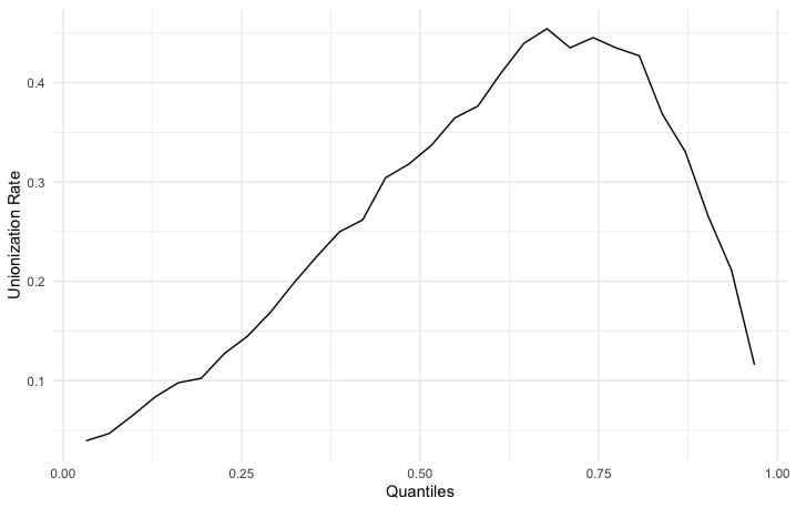
Figure 2: Unionization rates by quantiles of the distribution of wages.

5.1 Global effect and bounds

Consider a policy that increase in the unionization rate by $10\%$. It consists of unionizing workers whose wages are below the $.10/(1-p)$-quantile $\approx 0.14$-quantile of the wages of the nonunionized sector. In the notation of this paper, we have $D=1$ if a worker is unionized, $D_{\delta}=1$ if a worker is unionized under the policy, $Y$ is (log) wage, and $\delta=0.1$. That is, $D_{\delta}$ is given by

$$D_{\delta}=\begin{cases}1&\quad\text{if }D=1\\ 1&\quad\text{if }D=0\text{ and }Y\leq F^{-1}_{Y|D=0}(0.14)\\ 0&\quad\text{otherwise}\\ \end{cases}$$

Figure 3 shows the quantile breakdown frontiers for $g=0.1$ for a grid of $\tau\in(0.15,0.85)$. Confidence intervals are obtained via 1,000 bootstrap replications. Since the outcome variable is log wages, this means approximately a $10\%$ increase in wages. First, we can see that for lower quantiles, the conclusion will hold as long as $c$ is below the frontier. On the other hand, for upper quantiles, the conclusion does not hold under point identification. Thus there is no point in doing a sensitivity analysis for upper quantiles.

Suppose the policy maker is interested in $\tau^{*}=.3$. In this case, $c_{\tau^{*},L}=c_{.3,L}=0.29$, and $[0.27,0.30]$ is the $95\%$ confidence interval. Importantly, $\tilde{F}_{A}^{-1}(\tau-\delta)<F_{A}^{-1}(\tau-\delta c_{\tau^{*},L})$, meaning that the conclusion does not hold for any $c\in[0,1]$ by part $(iv)$ of Lemma 1, and hence the quantile breakdown frontier is sharp at $\tau=.3$. Using equation (8), we can find the bounds for the global effect for all quantiles which are consistent with this amount of policy selection bias. This is shown in Figure 4. Note that at $\tau=0.3$, the lower bound is $.10$ by construction. At upper quantiles, the lower bound is slightly negative.

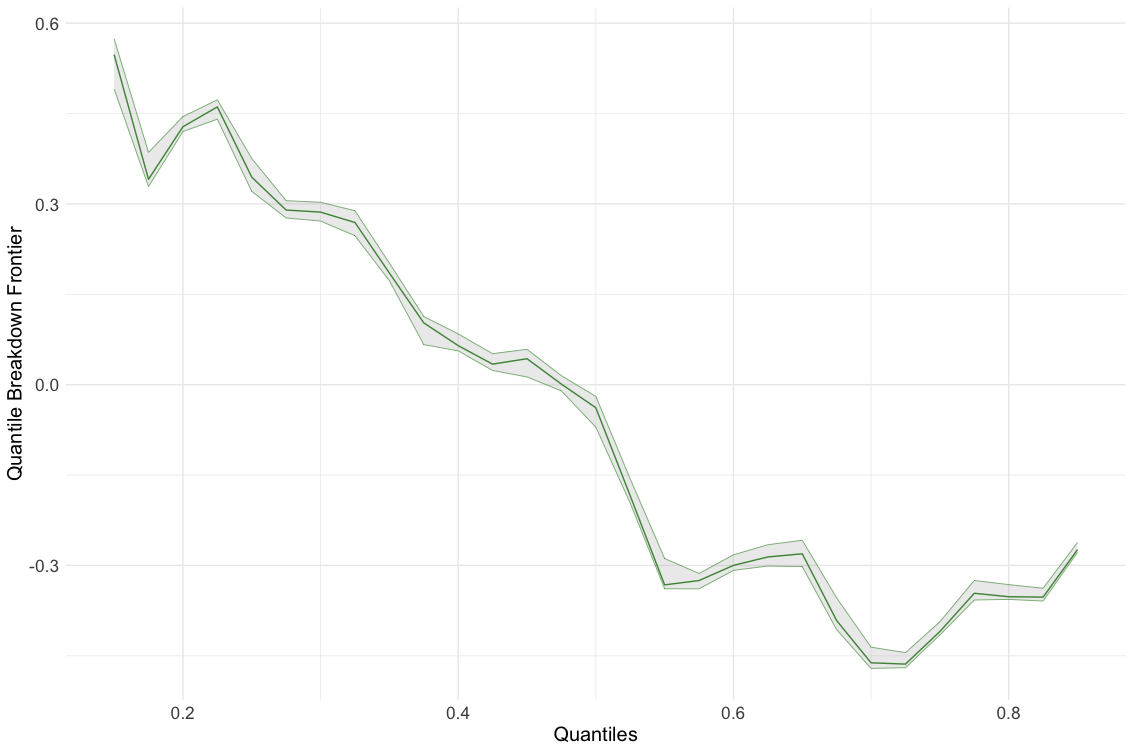
Figure 3: Quantile Breakdown Frontier for $G_{\tau,D_{\delta}}\geq 0.1$ with $95\%$ pointwise confidence intervals.

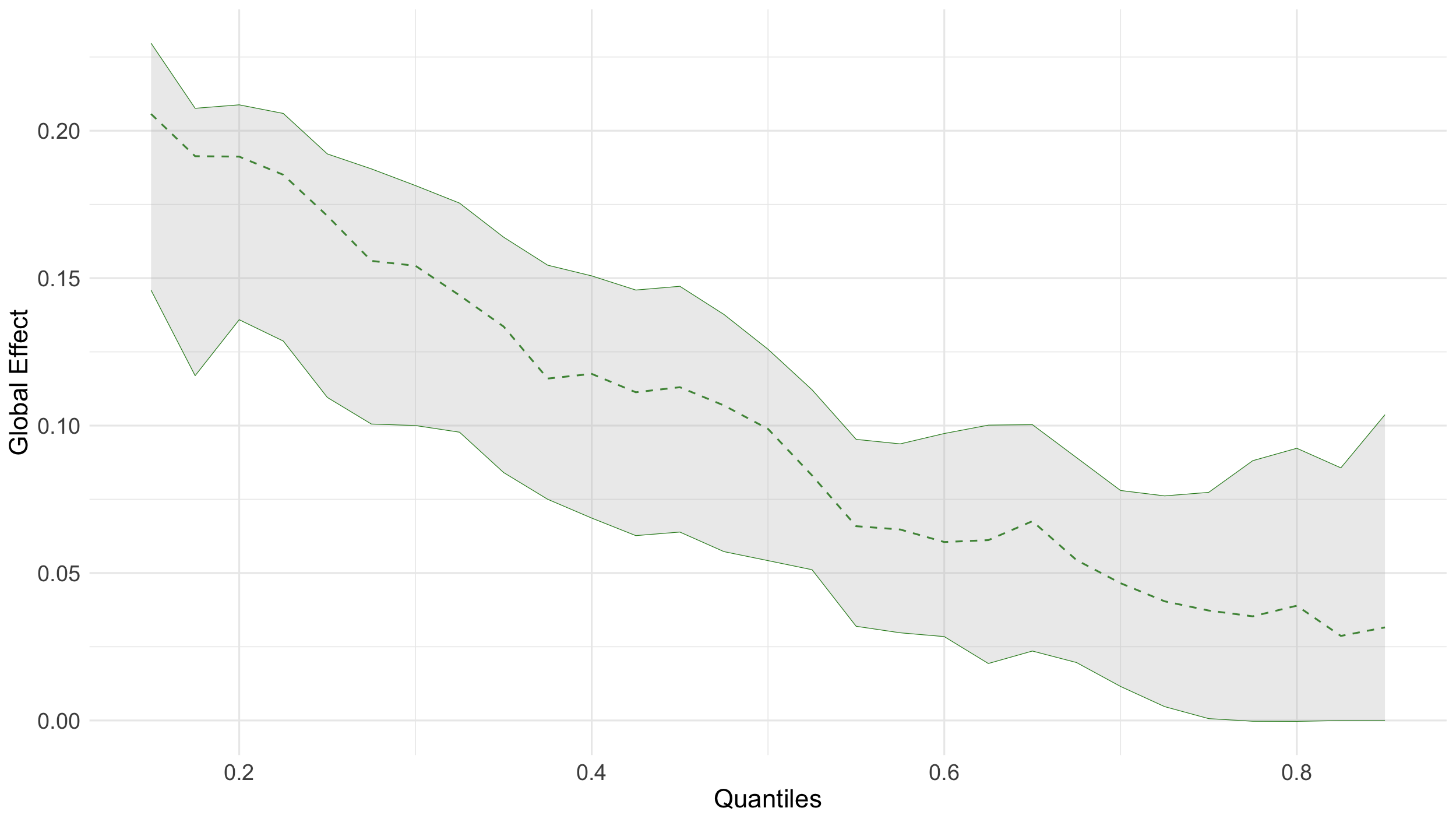
Figure 4: Bounds derived from the QBF, and (dashed) point identified global effect.

6 Conclusion

This paper provides a way to perform a sensitivity analysis on the unconditional quantiles effects of policies that manipulate the proportion of treated individuals. To do so, we introduce the quantile breakdown frontier as a tool to examine, across quantiles, whether a sensitivity analysis is possible, and how much policy selection bias is compatible with a given conclusion. Next, we use the information from the curve at a particular quantile to provide bounds on the effect of a policy across quantiles. Our empirical application looks at the effect of increasing the proportion of unionized workers by unionizing lower earners. We find that an increase of $10\%$ for the $30$^th quantile is consistent under moderate values of selection bias. Moreover, this implies that the effect on lower quantiles would be even bigger, and that lower quantiles would not be hurt.

Appendices

A Notation for Estimation and Inference

For $F_{A}(y)$ given in Theorem 1, $\hat{F}_{A}(y)$ is its empirical counterpart. It is given by

$$\hat{F}_{A}(y) :=\hat{p}\hat{F}_{Y|D=1}(y)+(1-\hat{p}-\delta)\hat{F}_{Y|D_{\delta}=0}(y)+\delta\sum_{x\in\mathcal{X}}\hat{F}_{Y|D=1,X=x}(y)\hat{p}_{x}$$ (A.1)

where $p_{x}:=\Pr(X=x|D=0,D_{\delta}=1)$ and

$$\hat{p}_{x} =\frac{\sum_{i=1}^{n}\mathds{1}\left\{X_{i}=x\right\}(1-D_{i})(1-D_{i,\delta})}{\sum_{i=1}^{n}(1-D_{i})(1-D_{i,\delta})},$$

$$\hat{p} =\frac{1}{n}\sum_{i=1}^{n}D_{i},$$

$$\hat{F}_{Y|D=1}(y) =\frac{\sum_{i=1}^{n}\mathds{1}\left\{Y_{i}\leq y\right\}D_{i}}{\sum_{i=1}^{n}D_{i}},$$

$$\hat{F}_{Y|D_{\delta}=0}(y) =\frac{\sum_{i=1}^{n}\mathds{1}\left\{Y_{i}\leq y\right\}(1-D_{i,\delta})}{\sum_{i=1}^{n}(1-D_{i,\delta})},$$

$$\hat{F}_{Y|D=1,X=x}(y) =\frac{\sum_{i=1}^{n}\mathds{1}\left\{Y_{i}\leq y\right\}D_{i}\mathds{1}\left\{X_{i}=x\right\}}{\sum_{i=1}^{n}D_{i}\mathds{1}\left\{X_{i}=x\right\}}.$$

Moreover, we have

$$\hat{\tilde{F}}_{A}(y) :=\hat{p}\hat{F}_{Y|D=1}(y)+(1-\hat{p}-\delta)\hat{F}_{Y|D_{\delta}=0}(y).$$ (A.2)

For the marginal effect, we have the following empirical cdf:

$$\hat{F}_{Y|D=0}(y)=\frac{\sum_{i=1}^{n}\mathds{1}\{Y_{i}\leq y\}(1-D_{i})}{\sum_{i=1}^{n}((1-D_{i}))}.$$

and

$$\sum_{x\in\mathcal{X}}\hat{F}_{Y|D=1,X=x}(y)\hat{p}_{x|\partial D}=\sum_{x\in\mathcal{X}}\frac{\sum_{i=1}^{n}\mathds{1}\left\{Y_{i}\leq y\right\}D_{i}\mathds{1}\left\{X_{i}=x\right\}}{\sum_{i=1}^{n}D_{i}\mathds{1}\left\{X_{i}=x\right\}}\hat{p}_{x|\partial D}.$$

B Proofs

Proof of Theorem 1.

Recall that, for a given $D_{\delta}$, the counterfactual distribution is

$$F_{Y_{D_{\delta}}}(y) =pF_{Y|D=1}(y)+(1-p-\delta)F_{Y|D_{\delta}=0}(y)+\delta F_{Y(1)|D=0,D_{\delta}=1}(y).$$

Since $F_{Y(1)|D=0,D_{\delta}=1}$ is a distribution function, we naturally have $0\leq F_{Y(1)|D=0,D_{\delta}=1}(y)\leq 1$ for every $y\in\mathbb{R}$. Moreover, by Assumption 3, we also have that

$$\int_{\mathcal{X}}F_{Y|D=1,X=x}(y)dF_{X|D=0,D_{\delta}=1}(x)-c\leq F_{Y(1)|D=0,D_{\delta}=1}(y)\leq\int_{\mathcal{X}}F_{Y|D=1,X=x}(y)dF_{X|D=0,D_{\delta}=1}(x)+c$$

$y\in\mathbb{R}$. Thus combining both bounds, we obtain

$$\max\left\{0,\int_{\mathcal{X}}F_{Y|D=1,X=x}(y)dF_{X|D=0,D_{\delta}=1}(x)-c\right\} \leq F_{Y(1)|D=0,D_{\delta}=1}(y)$$

$$\leq\min\left\{1,\int_{\mathcal{X}}F_{Y|D=1,X=x}(y)dF_{X|D=0,D_{\delta}=1}(x)+c\right\}.$$

for every $y\in\mathbb{R}$. To help with the notation, define

$$\tilde{F}_{A}(y) :=pF_{Y|D=1}(y)+(1-p-\delta)F_{Y|D_{\delta}=0}(y),$$ (A.3)

and

$$F_{A}(y) :=\tilde{F}_{A}(y)+\delta\int_{\mathcal{X}}F_{Y|D=1,X=x}(y)dF_{X|D=0,D_{\delta}=1}(x).$$ (A.4)

Note that, while $F_{A}(y)$ is a proper distribution function, $\tilde{F}_{A}(y)$ is not. We refer to $F_{A}$ as the apparent distribution, and to $\tilde{F}_{A}$ as the incomplete apparent distribution. By Assumption 2, both $F_{A}(y)$ and $\tilde{F}_{A}(y)$ are strictly increasing and continuous on for all $y$ such that $0<F_{A}(y)<1$ and $0<\tilde{F}_{A}(y)<1$. The bounds on $F_{Y(1)|D=0,D_{\delta}=1}(y)$, allow us to bound $F_{Y_{D_{\delta}}}(y)$. The upper bound is

$$F_{Y_{D_{\delta}}}(y) \leq pF_{Y|D=1}(y)+(1-p-\delta)F_{Y|D_{\delta}=0}(y)$$

$$+\delta\min\left\{1,\int_{\mathcal{X}}F_{Y|D=1,X=x}(y)dF_{X|D=0,D_{\delta}=1}(x)+c\right\}$$

$$=\min\left\{\tilde{F}_{A}(y)+\delta,F_{A}(y)+\delta c\right\}.$$

Similarly, the lower bound is

$$F_{Y_{D_{\delta}}}(y) \geq pF_{Y|D=1}(y)+(1-p-\delta)F_{Y|D_{\delta}=0}(y)$$

$$+\delta\max\left\{0,\int_{\mathcal{X}}F_{Y|D=1,X=x}(y)dF_{X|D=0,D_{\delta}=1}(x)-c\right\}$$

$$=\max\left\{\tilde{F}_{A}(y),F_{A}(y)-\delta c\right\}.$$

Let $F_{Y_{D_{\delta}}}^{-1}(\tau)$ be that $\tau$-quantile of $Y_{D_{\delta}}$ which is unique by Assumption 2. Then

$$\max\left\{\tilde{F}_{A}(F_{Y_{D_{\delta}}}^{-1}(\tau)),F_{A}(F_{Y_{D_{\delta}}}^{-1}(\tau))-\delta c\right\}\leq\tau\leq\min\left\{\tilde{F}_{A}(F_{Y_{D_{\delta}}}^{-1}(\tau))+\delta,F_{A}(F_{Y_{D_{\delta}}}^{-1}(\tau))+\delta c\right\}.$$

For two strictly increasing increasing continuous functions $f$ and $g$, we have that (this is best seen graphically):

$$\left[\min\left\{f,g\right\}\right]^{-1}(\tau)=\max\left\{f^{-1}(\tau),g^{-1}(\tau)\right\}.$$

and

$$\left[\max\left\{f,g\right\}\right]^{-1}(\tau)=\min\left\{f^{-1}(\tau),g^{-1}(\tau)\right\}.$$

Moreover, for $F_{A}$, define the inverse to be $F_{A}^{-1}(t)$, where $F_{A}(F_{A}^{-1}(t))=t$ for $t\in(0,1)$, $F_{A}^{-1}(t)=-\infty$ if $t\leq 0$, and $F_{A}^{-1}(t)=\infty$ if $t\geq 1$. For the “incomplete” apparent distribution $\tilde{F}_{A}$, we have that $\tilde{F}_{A}:\mathbb{R}\mapsto(0,1-\delta)$. Thus, $\tilde{F}_{A}^{-1}(t)$ is defined as usual for $t\in(0,1-\delta)$. Whereas, $\tilde{F}_{A}^{-1}(t)=-\infty$ if $t\leq 0$, and $\tilde{F}_{A}^{-1}(t)=\infty$ if $t\geq 1-\delta$.

Thus, we can bound $F_{Y_{D_{\delta}}}^{-1}(\tau)$ by

$$\theta_{L}:=\max\left\{\tilde{F}_{A}^{-1}(\tau-\delta),F_{A}^{-1}(\tau-\delta c)\right\}\leq F_{Y_{D_{\delta}}}^{-1}(\tau)\leq\min\left\{\tilde{F}_{A}^{-1}(\tau),F_{A}^{-1}(\tau+\delta c)\right\}:=\theta_{H}.$$

Since we restrict $\tau$ to $(\delta,1-\delta)$, for any $c\in[0,1)$, then $\theta_{L}>-\infty$ and $\theta_{H}<\infty.$ To show that the bounds are sharp we follow the approach of the proof of Lemma 2.1 of Kline and Santos (2013). For any value that $F_{Y_{D_{\delta}}}^{-1}(\tau)$ may take in $[\theta_{L},\theta_{H}]$, we need to show that there exists a function $F^{*}_{\delta}:\mathbb{R}\mapsto(0,1)$ such that:

1. $\tau=pF_{Y|D=1}(F_{Y_{D_{\delta}}}^{-1}(\tau))+(1-p-\delta)F_{Y|D_{\delta}=0}(F_{Y_{D_{\delta}}}^{-1}(\tau))+\delta F^{*}_{\delta}(F_{Y_{D_{\delta}}}^{-1}(\tau))$;

2. $\sup_{y\in\mathbb{R}}\left|F^{*}_{\delta}(y)-\int_{\mathcal{X}}F_{Y|D=1,X=x}(y)dF_{X|D=0,D_{\delta}=1}(x)\right|\leq c$;

3. $F^{*}_{\delta}(y)$ is continuous and strictly increasing in $\mathbb{R}$ for all $y$ such that $0<F^{*}_{\delta}(y)<1.$

By condition 1., we can express $F^{*}_{\delta}(F_{Y_{D_{\delta}}}^{-1}(\tau))$ as

$$F^{*}_{\delta}(F_{Y_{D_{\delta}}}^{-1}(\tau))=\frac{\tau-pF_{Y|D=1}(F_{Y_{D_{\delta}}}^{-1}(\tau))-(1-p-\delta)F_{Y|D_{\delta}=0}(F_{Y_{D_{\delta}}}^{-1}(\tau))}{\delta}$$

To verify condition 2., we start by checking that $\left|F^{*}_{\delta}(F_{Y_{D_{\delta}}}^{-1}(\tau))-\int_{\mathcal{X}}F_{Y|D=1,X=x}(F_{Y_{D_{\delta}}}^{-1}(\tau))dF_{X|D=0,D_{\delta}=1}(x)\right|\leq c$. We write

$$F^{*}_{\delta}(F_{Y_{D_{\delta}}}^{-1}(\tau))-\int_{\mathcal{X}}F_{Y|D=1,X=x}(F_{Y_{D_{\delta}}}^{-1}(\tau))dF_{X|D=0,D_{\delta}=1}(x) =\frac{\tau-pF_{Y|D=1}(F_{Y_{D_{\delta}}}^{-1}(\tau))-(1-p-\delta)F_{Y|D_{\delta}=0}(F_{Y_{D_{\delta}}}^{-1}(\tau))}{\delta}$$

$$-\int_{\mathcal{X}}F_{Y|D=1,X=x}(F_{Y_{D_{\delta}}}^{-1}(\tau))dF_{X|D=0,D_{\delta}=1}(x)$$

$$=\frac{\tau-F_{A}(F_{Y_{D_{\delta}}}^{-1}(\tau))}{\delta}.$$

Because $F_{A}$ is increasing, and $F_{Y_{D_{\delta}}}^{-1}(\tau)\in[\theta_{L},\theta_{H}]$, we need to check all the possible limiting cases.

1. $F_{Y_{D_{\delta}}}^{-1}(\tau)=F_{A}^{-1}(\tau-\delta c)$. Then,

   $$\frac{\tau-F_{A}(F_{A}^{-1}(\tau-\delta c))}{\delta}=c.$$

2. $F_{Y_{D_{\delta}}}^{-1}(\tau)=\tilde{F}_{A}^{-1}(\tau-\delta)$. Then,

   $$\frac{\tau-F_{A}(\tilde{F}_{A}^{-1}(\tau-\delta))}{\delta}\leq\frac{\tau-F_{A}(F_{A}^{-1}(\tau-\delta c))}{\delta}=c,$$

   where the inequality follows from $\tilde{F}_{A}^{-1}(\tau-\delta)\geq F_{A}^{-1}(\tau-\delta c)$.

3. $F_{Y_{D_{\delta}}}^{-1}(\tau)=F_{A}^{-1}(\tau+\delta c)$. Then,

   $$\frac{\tau-F_{A}(F_{A}^{-1}(\tau+\delta c))}{\delta}=-c.$$

4. $F_{Y_{D_{\delta}}}^{-1}(\tau)=\tilde{F}_{A}^{-1}(\tau)$. Then,

   $$\frac{\tau-F_{A}(\tilde{F}_{A}^{-1}(\tau))}{\delta}\geq\frac{\tau-F_{A}(F_{A}^{-1}(\tau+\delta c))}{\delta}=-c,$$

   where the inequality follows from $\tilde{F}_{A}^{-1}(\tau)\leq F_{A}^{-1}(\tau+\delta c)$.

Thus, we have that $\left|F^{*}_{\delta}(F_{Y_{D_{\delta}}}^{-1}(\tau))-\int_{\mathcal{X}}F_{Y|D=1,X=x}(F_{Y_{D_{\delta}}}^{-1}(\tau))dF_{X|D=0,D_{\delta}=1}(x)\right|\leq c$ whenever $F_{Y_{D_{\delta}}}^{-1}(\tau)\in[\theta_{L},\theta_{H}]$.

Now we will construct $F^{*}_{\delta}(y)$ such that conditions 2. and 3. also hold. The starting point is the given value $F^{*}_{\delta}(F_{Y_{D_{\delta}}}^{-1}(\tau))$. To alleviate notation, define

$$\tilde{F}(y):=\int_{\mathcal{X}}F_{Y|D=1,X=x}(y)dF_{X|D=0,D_{\delta}=1}(x)$$

Suppose first that

$$F^{*}_{\delta}(F_{Y_{D_{\delta}}}^{-1}(\tau))\leq\tilde{F}(F_{Y_{D_{\delta}}}^{-1}(\tau))$$

Then, we define $F^{*}_{\delta}(y)$ as

$$F^{*}_{\delta}(y)=\begin{cases}\max\left\{0,\tilde{F}(y)-\left[\tilde{F}(F_{Y_{D_{\delta}}}^{-1}(\tau))-F^{*}_{\delta}(F_{Y_{D_{\delta}}}^{-1}(\tau))\right]\right\}\text{ for }y\leq F_{Y_{D_{\delta}}}^{-1}(\tau)\\ \tilde{F}(y)-\omega(y-F_{Y_{D_{\delta}}}^{-1}(\tau))\left[\tilde{F}(F_{Y_{D_{\delta}}}^{-1}(\tau))-F^{*}_{\delta}(F_{Y_{D_{\delta}}}^{-1}(\tau))\right]\text{ for }y>F_{Y_{D_{\delta}}}\\ \end{cases}$$

where $\omega(y)$ is a continuous function that satisfies: $\omega(0)=1$, $\lim_{y\to\pm\infty}\omega(y)=0$, and it is strictly decreasing for $y>0$, and strictly increasing for $y<0$. We can take $\omega(y)=\exp(-y^{2})$. The role of $\omega(y)$ is that of a weighting function. It brings $F^{*}_{\delta}(y)$ closer to $\tilde{F}(y)$ as we move to the right of $F_{Y_{D_{\delta}}}^{-1}(\tau)$. Since $\omega(y)\to 0$ as $y\to 0$, eventually the gap disappears. For the values of $y$ to the left of $F_{Y_{D_{\delta}}}^{-1}(\tau)$, we simply subtract the gap and use the $\max$ to keep the function non-negative. This function $F^{*}_{\delta}(y)$ satisfies 1., 2., and 3.

If, instead,

$$F^{*}_{\delta}(F_{Y_{D_{\delta}}}^{-1}(\tau))\geq\tilde{F}(F_{Y_{D_{\delta}}}^{-1}(\tau))$$

then

$$F^{*}_{\delta}(y)=\begin{cases}\tilde{F}(y)-\omega(y-F_{Y_{D_{\delta}}}^{-1}(\tau))\left[\tilde{F}(F_{Y_{D_{\delta}}}^{-1}(\tau))-F^{*}_{\delta}(F_{Y_{D_{\delta}}}^{-1}(\tau))\right]\text{ for }y\leq F_{Y_{D_{\delta}}}\\ \min\left\{1,\tilde{F}(y)-\left[\tilde{F}(F_{Y_{D_{\delta}}}^{-1}(\tau))-F^{*}_{\delta}(F_{Y_{D_{\delta}}}^{-1}(\tau))\right]\right\}\text{ for }y>F_{Y_{D_{\delta}}}^{-1}(\tau)\\ \end{cases}$$

Here, $F^{*}_{\delta}(y)$ lies above $\tilde{F}(y)$ and we use the weight function to close the gap as $y\to-\infty.$ For the values of $y>F_{Y_{D_{\delta}}}^{-1}(\tau)$ we simply add the gap (we are subtracting a negative number) and use the $\min$ to avoid the function from being greater than 1. This function $F^{*}_{\delta}(y)$ satisfies 1., 2., and 3.

Therefore, sharp bounds for the global effect $G_{\tau,D_{\delta}}:=F_{Y_{D_{\delta}}}^{-1}(\tau)-F_{Y}^{-1}(\tau)$, are given by

$$\max\left\{\tilde{F}_{A}^{-1}(\tau-\delta),F_{A}^{-1}(\tau-\delta c)\right\}-F_{Y}^{-1}(\tau)\leq G_{\tau,D_{\delta}}\leq\min\left\{\tilde{F}_{A}^{-1}(\tau),F_{A}^{-1}(\tau+\delta c)\right\}-F_{Y}^{-1}(\tau).$$

∎

Proof of Theorem 2.

Recall that by (3), the counterfactual distribution of a given policy $D_{\delta}$ that satisfies assumption 1 is

$$F_{Y_{D_{\delta}}}(y) =pF_{Y|D=1}(y)+(1-p-\delta)F_{Y|D_{\delta}=0}(y)+\delta F_{Y(1)|D=0,D_{\delta}=1}(y)$$

Then, we can write the quotient as

$$\frac{F_{Y_{D_{\delta}}}(y)-F_{Y}(y)}{\delta} =(1-p)\frac{F_{Y|D_{\delta}=0}(y)-F_{Y|D=0}(y)}{\delta}-F_{Y|D_{\delta}=0}(y)+F_{Y(1)|D=0,D_{\delta}=1}(y).$$

By Assumption 4, we can take the limit $\delta\downarrow 0$ to obtain

$$\lim_{\delta\downarrow 0}\frac{F_{Y_{D_{\delta}}}(y)-F_{Y}(y)}{\delta} =(1-p)\frac{\partial F_{Y|D_{\delta}=0}(y)}{\partial\delta}\bigg{|}_{\delta=0}-F_{Y|D=0}(y)+F_{Y(1)|\partial D}(y)$$

$$=:\dot{F}_{Y,\mathcal{D}}(y).$$

The map $y\mapsto\dot{F}_{Y,\mathcal{D}}(y)$ is continuous by Assumption 4. Now we aim to strengthen the pointwise result to a uniform result. For that, we write:

$$\sup_{y\in\mathbb{R}}\left|\frac{F_{Y_{D_{\delta}}}(y)-F_{Y}(y)}{\delta}-\dot{F}_{Y,\mathcal{D}}(y)\right| \leq(1-p)\sup_{y\in\mathbb{R}}\left|\frac{F_{Y|D_{\delta}=0}(y)-F_{Y|D=0}(y)}{\delta}-\frac{\partial F_{Y|D_{\delta}=0}(y)}{\partial\delta}\bigg{|}_{\delta=0}\right|$$

$$+\sup_{y\in\mathbb{R}}\left|F_{Y|D_{\delta}=0}(y)-F_{Y|D=0}(y)\right|$$

$$+\sup_{y\in\mathbb{R}}\left|F_{Y(1)|D=0,D_{\delta}=1}(y)-F_{Y(1)|\partial D}(y)\right|$$

Assumption 4 ensures the uniform convergence of the first and third summands. The second summand convergence uniformly because it is analogous to weak convergence to a continuous distribution function (see Exercise 5.(b) in Chapter 8 of Resnick (2005)).

Finally, let $\Gamma_{\tau}[F]$ be the $\tau$-quantile of $F$. The Hadamard derivative at $F$ is (see Lemma 21.3 in van der Vaart (1998))

$$\Gamma_{\tau,F}^{\prime}[h]=-\frac{h(F^{-1}(\tau))}{f(F^{-1}(\tau))}.$$

for any $h\in\mathbb{D}[-\infty,\infty]$ continuous at $F^{-1}(\tau)$. We write the marginal effect as

$$M_{\tau,\mathcal{D}} =\lim_{\delta\to 0}\frac{\Gamma_{\tau}\left[F_{Y_{D_{\delta}}}\right]-\Gamma_{\tau}[F_{Y}]}{\delta}=\lim_{\delta\to 0}\frac{\Gamma_{\tau}\left[F_{Y_{D_{0}}}+\delta\left(\frac{F_{Y_{D_{\delta}}}-F_{Y_{D_{0}}}}{\delta}\right)\right]-\Gamma_{\tau}[F_{Y}]}{\delta}$$

$$=\lim_{\delta\to 0}\frac{\Gamma_{\tau}\left[F_{Y}+\delta\left(\frac{F_{Y_{D_{\delta}}}-F_{Y}}{\delta}\right)\right]-\Gamma_{\tau}[F_{Y}]}{\delta}$$

$$=\Gamma_{\tau,F_{Y}}^{\prime}[\dot{F}_{Y,\mathcal{D}}]=\frac{\dot{F}_{Y,\mathcal{D}}(F_{Y}^{-1}(\tau))}{f_{Y}(F_{Y}^{-1}(\tau))}.$$

The third equality follows from $F_{Y_{D_{0}}}=F_{Y}$. This is because by (3), and the fact we have assumed that $\lim_{\delta\to 0}F_{Y|D_{\delta}=0}=F_{Y|D=0}$ and that $\lim_{\delta\to 0}F_{Y(1)|D=0,D_{\delta}=1}$ is well defined. The fourth equality follows from

$$\lim_{\delta\downarrow 0}\sup_{y\in\mathcal{Y}}\left|\frac{F_{Y_{D_{\delta}}}(y)-F_{Y}(y)}{\delta}-\dot{F}_{Y,\mathcal{D}}(y)\right|=0,$$

which is required by Lemma 21.3 in van der Vaart (1998).

∎

Details of 3.

Let $D=\mathds{1}\left\{V\geq 0\right\}$ for $V$ continuously distributed around 0, and, for a sequence $\delta\downarrow 0$, let $D_{\delta}=\mathds{1}\left\{V\geq F_{V}^{-1}(F_{V}(0)-\delta)\right\}$. It follows that $p:=\Pr(D=1)=1-F_{V}(0)$ and that $\Pr(D_{\delta}=1)=p+\delta$. Suppose that $\lim_{\delta\to 0}\Pr(Y\leq y|V\leq F_{V}^{-1}(F_{V}(0)-\delta))=\Pr(Y\leq y|V\leq 0)$. Then

$$\lim_{\delta\to 0}F_{Y|D_{\delta}=0}(y) =\lim_{\delta\to 0}\Pr(Y\leq y|V\leq F_{V}^{-1}(F_{V}(0)-\delta))$$

$$=\Pr(Y\leq y|V\leq 0)$$

$$=F_{Y|D=0}(y).$$

Now, we have

$$F_{Y|D_{\delta}=0}(y)-F_{Y|D=0}(y) =\frac{\Pr(Y\leq y,V\leq F_{V}^{-1}(F_{V}(0)-\delta))}{p+\delta}-\frac{\Pr(Y\leq y,V\leq 0)}{p}$$

$$= \frac{p\Pr(Y\leq y,V\leq F_{V}^{-1}(F_{V}(0)-\delta))-(p+\delta)\Pr(Y\leq y,V\leq 0)}{(p+\delta)p}$$

$$=\frac{1}{p+\delta}\left[\Pr(Y\leq y,V\leq F_{V}^{-1}(F_{V}(0)-\delta))-\Pr(Y\leq y,V\leq 0)\right]$$

$$-\frac{\delta}{p(p+\delta)}\Pr(Y\leq y,V\leq 0)$$

Consider the first term:

$$\frac{\Pr(Y\leq y,V\leq F_{V}^{-1}(F_{V}(0)-\delta))-\Pr(Y\leq y,V\leq 0)}{\delta} =\frac{F_{V}^{-1}(F_{V}(0)-\delta)}{\delta}$$

$$\times\frac{\Pr(Y\leq y,V\leq F_{V}^{-1}(F_{V}(0)-\delta))-\Pr(Y\leq y,V\leq 0)}{F_{V}^{-1}(F_{V}(0)-\delta)}$$

Now, provided that $f_{V}(0)\neq 0$,

$$\lim_{\delta\to 0}\frac{F_{V}^{-1}(F_{V}(0)-\delta)}{\delta}=-\frac{1}{f_{V}(0)}.$$

For the other term we have

$$\frac{\Pr(Y\leq y,V\leq F_{V}^{-1}(F_{V}(0)-\delta))-\Pr(Y\leq y,V\leq 0)}{F_{V}^{-1}(F_{V}(0)-\delta)} =\frac{\int^{F_{V}^{-1}(F_{V}(0)-\delta)}_{0}\int_{-\infty}^{y}f_{Y,V}(u,v)dudv}{F_{V}^{-1}(F_{V}(0)-\delta)}$$

$$\to\int_{-\infty}^{y}f_{Y,V}(u,0)du$$

Combining all together, we obtain

$$\lim_{\delta\to 0}\frac{F_{Y|D_{\delta}=0}(y)-F_{Y|D=0}(y)}{\delta}=-\left(\frac{1}{f_{V}(0)}+\frac{1}{p}\right)F_{Y|D=0}(y)$$

Thus we can take

$$\frac{\partial F_{Y|D_{\delta}=0}(y)}{\partial\delta}\bigg{|}_{\delta=0}=-\left(\frac{1}{f_{V}(0)}-\frac{1}{p}\right)F_{Y|D=0}(y)$$

which will be continuous as long as $F_{Y|D=0}(y)$ is continuous (which we assumed). Now, consider

$$F_{Y(1)|D=0,D_{\delta}=1}(y) =\Pr(Y(1)\leq y|V\leq 0,V\geq F_{V}^{-1}(F_{V}(0)-\delta))$$

$$=\frac{\Pr(Y(1)\leq y,V\leq 0,V\geq F_{V}^{-1}(F_{V}(0)-\delta))}{\Pr(V\leq 0,V\geq F_{V}^{-1}(F_{V}(0)-\delta))}$$

$$=\frac{\int_{F_{V}^{-1}(F_{V}(0)-\delta)}^{0}\int_{-\infty}^{0}f_{Y(1),V}(u,v)dudv}{\delta}$$

$$=\frac{F_{V}^{-1}(F_{V}(0)-\delta)}{\delta}\frac{\int_{F_{V}^{-1}(F_{V}(0)-\delta)}^{0}\int_{-\infty}^{0}f_{Y(1),V}(u,v)dudv}{F_{V}^{-1}(F_{V}(0)-\delta)}.$$

Under some mild regularity conditions:

$$\lim_{\delta\to 0}F_{Y(1)|D=0,D_{\delta}=1}(y)=F_{Y(1)|V=0}(y)$$

Thus, we can take

$$F_{Y(1)|\partial D}(y)=F_{Y(1)|V=0}(y).$$

∎

Proof of Theorem 3.

To bound the marginal effect, which we assume that exists, we aim to take the limit when $\delta\downarrow 0$ of the rescaled bounds of the global effect. That is, we aim to bound the marginal effect by the limiting versions of

$$\frac{\max\left\{\tilde{F}_{A}^{-1}(\tau-\delta),F_{A}^{-1}(\tau-\delta c)\right\}-F_{Y}^{-1}(\tau)}{\delta},$$

and

$$\frac{\min\left\{\tilde{F}_{A}^{-1}(\tau),F_{A}^{-1}(\tau+\delta c)\right\}-F_{Y}^{-1}(\tau)}{\delta}.$$

We would like to show that, when $\delta\downarrow 0$, we have

$$\lim_{\delta\downarrow 0}\frac{\max\left\{\tilde{F}_{A}^{-1}(\tau-\delta),F_{A}^{-1}(\tau-\delta c)\right\}-F_{Y}^{-1}(\tau)}{\delta}\leq M_{\tau,\mathcal{D}}\leq\lim_{\delta\downarrow 0}\frac{\min\left\{\tilde{F}_{A}^{-1}(\tau),F_{A}^{-1}(\tau+\delta c)\right\}-F_{Y}^{-1}(\tau)}{\delta}$$

The reason we take the limit from the right, i.e. $\delta\downarrow 0$, is because twofold the ordinary limit might fail to exist. This is the reason why we assume that the sequence of policies consists of $\delta>0$ moving towards 0. This is part of Assumption 1. For $\delta>0$, we can write

$$\frac{\max\left\{\tilde{F}_{A}^{-1}(\tau-\delta),F_{A}^{-1}(\tau-\delta c)\right\}-F_{Y}^{-1}(\tau)}{\delta} =\frac{\max\left\{\tilde{F}_{A}^{-1}(\tau-\delta)-F_{Y}^{-1}(\tau),F_{A}^{-1}(\tau-\delta c)-F_{Y}^{-1}(\tau)\right\}}{\delta}$$

$$=\max\left\{\frac{\tilde{F}_{A}^{-1}(\tau-\delta)-F_{Y}^{-1}(\tau)}{\delta},\frac{F_{A}^{-1}(\tau-\delta c)-F_{Y}^{-1}(\tau)}{\delta}\right\}.$$

The last step, bringing $1/\delta$ into the $\max$, is only valid because $\delta>0$. Similarly, for $\delta>0$, we have

$$\frac{\min\left\{\tilde{F}_{A}^{-1}(\tau),F_{A}^{-1}(\tau+\delta c)\right\}-F_{Y}^{-1}(\tau)}{\delta}=\min\left\{\frac{\tilde{F}_{A}^{-1}(\tau)-F_{Y}^{-1}(\tau)}{\delta},\frac{F_{A}^{-1}(\tau+\delta c)-F_{Y}^{-1}(\tau)}{\delta}\right\}$$

Now, since the $\max$ and $\min$ are continuous, to pass the limit as $\delta\downarrow 0$ we need to show that the maps

$$\delta\mapsto\tilde{F}_{A}^{-1}(\tau-\delta),$$

$$\delta\mapsto F_{A}^{-1}(\tau-\delta c),$$

$$\delta\mapsto\tilde{F}_{A}^{-1}(\tau),$$

$$\delta\mapsto F_{A}^{-1}(\tau+\delta c),$$

are differentiable at $\delta=0$. We need to show differentiability because it follows from equations (A.3) and (A.4) that all these maps evaluated at $\delta=0$ are equal to $F_{Y}^{-1}(\tau)$. Provided they are differentiable (something we show below), we obtain:

$$\max\left\{\frac{\tilde{F}_{A}^{-1}(\tau-\delta)}{\partial\delta}\bigg{|}_{\delta=0},\frac{\partial F_{A}^{-1}(\tau-\delta c)}{\partial\delta}\bigg{|}_{\delta=0}\right\}\leq M_{\tau,\mathcal{D}}\leq\min\left\{\frac{\partial\tilde{F}_{A}^{-1}(\tau)}{\partial\delta}\bigg{|}_{\delta=0},\frac{\partial F_{A}^{-1}(\tau+\delta c)}{\partial\delta}\bigg{|}_{\delta=0}\right\}$$

We start with the map $\delta\mapsto F_{A}^{-1}(\tau-\delta c)$. By equations (A.3) and (A.4), when $\delta=0$ , $F_{A}=F_{Y}$. So, we want to find the limit as $\delta\downarrow 0$ of

$$\frac{F^{-1}_{A}(\tau-\delta c)-F_{Y}^{-1}(\tau)}{\delta}.$$ (A.5)

We note that $\delta$ plays a triple role in the previous expression. Using (A.4), we write $F_{A}(y)$ as

$$F_{A}(y;\delta_{1},\delta_{2})=pF_{Y|D=1}(y)+(1-p-\delta_{1})F_{Y|D_{\delta_{2}}=0}(y)+\delta_{1}\int_{\mathcal{X}}F_{Y|D=1,X=x}(y)dF_{X|D=0,D_{\delta_{2}}=1}(x)$$ (A.6)

and we define

$$g(\delta_{1},\delta_{2},\delta_{3})=F^{-1}_{A}(\tau-\delta_{3}c;\delta_{1},\delta_{2})$$

The map $\delta_{1}\mapsto g(\delta_{1},\delta_{2},\delta_{3})$ for a fixed $\delta_{2}$ and $\delta_{3}$ is the composition

$$\delta_{1}\in\mathbb{R}\overset{h}{\mapsto}F_{A}(\cdot;\delta_{1},\delta_{2})\in\mathbb{D}[-\infty,\infty]\overset{\Gamma}{\mapsto}F^{-1}_{A}(\tau-\delta_{3}c;\delta_{1},\delta_{2})\in\mathbb{R}.$$

The first map $h:\delta_{1}\in\mathbb{R}\mapsto F_{A}(\cdot;\delta_{1},\delta_{2})\in\mathbb{D}[-\infty,\infty]$ has Hadamard derivative given by

$$\int_{\mathcal{X}}F_{Y|D=1,X=x}(\cdot)dF_{X|D=0,D_{\delta_{2}}=1}(x)-F_{Y|D_{\delta_{2}}=0}(\cdot).$$

The second map has Hadamard derivative given by (See Lemma 21.3 in van der Vaart (1998))

$$\Gamma^{\prime}_{F_{A}(\cdot;\delta_{1},\delta_{2})}[G]=-\frac{G(F^{-1}_{A}(\tau-\delta_{3}c;\delta_{1},\delta_{2}))}{f_{A}(F^{-1}_{A}(\tau-\delta_{3}c;\delta_{1},\delta_{2});\delta_{1},\delta_{2})}.$$

for $G\in\mathbb{D}[-\infty,\infty]$ continuous at $F^{-1}_{A}(\tau-\delta_{3}c;\delta_{1},\delta_{2})$. Then, the derivative of the composite map $\delta_{1}\mapsto\Gamma\circ h(\delta_{1})$ is $\Gamma^{\prime}_{F_{A}(\cdot;\delta_{1},\delta_{2})}[h^{\prime}(\delta_{1})]$, which is at $\delta_{2}=\delta_{3}=0$

$$\frac{\partial F^{-1}_{A}(\tau;\delta_{1},0)}{\partial\delta_{1}}=-\frac{\int_{\mathcal{X}}F_{Y|D=1,X=x}(F^{-1}_{A}(\tau;\delta_{1},0))dF_{X|\partial D}(x)-F_{Y|D=0}(F^{-1}_{A}(\tau;\delta_{1},0))}{f_{A}(F^{-1}_{A}(\tau;\delta_{1},0);\delta_{1},0)}.$$

which is continuous at $\delta_{1}=0$.

The derivative of the second map $\delta_{2}\mapsto g(\delta_{1},\delta_{2},\delta_{3})$, for a fixed $\delta_{1}=\delta_{3}=0$ is exactly 0 because as (A.4) shows, $\delta_{1}$ multiplies the expression

$$-F_{Y|D_{\delta_{2}}}(y)+\int_{\mathcal{X}}F_{Y|D=1,X=x}(y)dF_{X|D=0,D_{\delta_{2}}=1}(x).$$

All of the terms in this expression are differentiable at $\delta_{2}=0$ by Assumption 5.

The derivative of the third map $\delta_{3}\mapsto g(\delta_{1},\delta_{2},\delta_{3})$, for a fixed $\delta_{1}=\delta_{2}=0$, can be obtained via the identity

$$F_{A}\left(F^{-1}_{A}(\tau-\delta_{3}c;\delta_{1},\delta_{2})\delta_{1},\delta_{2}\right)=\tau-\delta_{3}c.$$

Differentiating through with respect to $\delta_{3}$, we obtain at $\delta_{1}=\delta_{2}=0$

$$\frac{\partial F^{-1}_{A}(\tau-\delta_{3}c;0,0)}{\partial\delta_{3}}=-\frac{c}{f_{Y}(F_{Y}^{-1}(\tau-\delta_{3}c))}.$$

which is continuous with respect to $\delta_{3}$.

Therefore, all the partial derivatives of the map $(\delta_{1},\delta_{2},\delta_{3})\mapsto g(\delta_{1},\delta_{2},\delta_{3})$ exist and are continuous, hence the limit in (A.5) exists and is equal to

$$\lim_{\delta\to 0}\frac{F^{-1}_{A}(\tau-\delta c)-F_{Y}^{-1}(\tau)}{\delta} =\frac{\partial g(\delta_{1},0,0)}{\partial\delta_{1}}\bigg{|}_{\delta_{1}=0}+\frac{\partial g(0,\delta_{2},0)}{\partial\delta_{2}}\bigg{|}_{\delta_{2}=0}+\frac{\partial g(0,0,\delta_{3})}{\partial\delta_{3}}\bigg{|}_{\delta_{3}=0}$$

$$=-\frac{\int_{\mathcal{X}}F_{Y|D=1,X=x}(F^{-1}_{Y}(\tau))dF_{X|\partial D}(x)-F_{Y|D=0}(F^{-1}_{Y}(\tau))}{f_{Y}(F^{-1}_{Y}(\tau))}-\frac{c}{f_{Y}(F_{Y}^{-1}(\tau))}.$$

Analogous arguments can be used to obtain that

$$\lim_{\delta\to 0}\frac{F^{-1}_{A}(\tau+\delta c)-F_{Y}^{-1}(\tau)}{\delta} =-\frac{\int_{\mathcal{X}}F_{Y|D=1,X=x}(F^{-1}_{Y}(\tau))dF_{X|\partial D}(x)-F_{Y|D=0}(F^{-1}_{Y}(\tau))}{f_{Y}(F^{-1}_{Y}(\tau))}+\frac{c}{f_{Y}(F_{Y}^{-1}(\tau))}.$$

Now we turn our attention to the incomplete apparent distribution $\tilde{F}_{A}$ and the map $\delta\mapsto\tilde{F}^{-1}_{A}(\tau-\delta)$. By equation (A.3), the incomplete apparent distribution is given by

$$\tilde{F}_{A}(y;\delta_{1},\delta_{2}) :=pF_{Y|D=1}(y)+(1-p-\delta_{1})F_{Y|D_{\delta_{2}}=0}(y),$$

where, again, we index by $\delta_{1}$ and $\delta_{2}$ to emphasize the dual role played by $\delta.$ As before, we define

$$g(\delta_{1},\delta_{2},\delta_{3})=\tilde{F}^{-1}_{A}(\tau-\delta_{3};\delta_{1},\delta_{2}).$$

The map $\delta_{1}\mapsto g(\delta_{1},\delta_{2},\delta_{3})$ for a fixed $\delta_{2}$ and $\delta_{3}$ is the composition

$$\delta_{1}\in\mathbb{R}\overset{h}{\mapsto}\tilde{F}_{A}(\cdot;\delta_{1},\delta_{2})\in\mathbb{D}[-\infty,\infty]\overset{\Gamma}{\mapsto}\tilde{F}^{-1}_{A}(\tau-\delta_{3};\delta_{1},\delta_{2})\in\mathbb{R}.$$

The first map $h:\delta_{1}\in\mathbb{R}\mapsto\tilde{F}_{A}(\cdot;\delta_{1},\delta_{2})\in\mathbb{D}[-\infty,\infty]$ has Hadamard derivative given by

$$-F_{Y|D_{\delta_{2}}=0}(\cdot).$$

The second map has Hadamard derivative given by

$$\Gamma^{\prime}_{\tilde{F}_{A}(\cdot;\delta_{1},\delta_{2})}[G]=-\frac{G(\tilde{F}^{-1}_{A}(\tau-\delta_{3}c;\delta_{1},\delta_{2}))}{\tilde{f}_{A}(\tilde{F}^{-1}_{A}(\tau-\delta_{3};\delta_{1},\delta_{2});\delta_{1},\delta_{2})}.$$

Then, the derivative of $\delta_{1}\mapsto\Gamma\circ h(\delta_{1})$ is $\Gamma^{\prime}_{\tilde{F}_{A}(\cdot;\delta_{1},\delta_{2})}[h^{\prime}(\delta_{1})]$, which is at $\delta_{2}=\delta_{3}=0$

$$\frac{\partial\tilde{F}^{-1}_{A}(\tau;\delta_{1},0)}{\partial\delta_{1}}=\frac{F_{Y|D=0}(\tilde{F}^{-1}_{A}(\tau;\delta_{1},0))}{\tilde{f}_{A}(\tilde{F}^{-1}_{A}(\tau;\delta_{1},0);\delta_{1},0)}$$

which is continuous at $\delta_{1}=0$.

The derivative of the second map $\delta_{2}\mapsto g(\delta_{1},\delta_{2},\delta_{3})$, for a fixed $\delta_{1}=\delta_{3}=0$ is exactly 0 because, as in the case of the (complete) apparent distribution, as (A.3) shows, $\delta_{1}$ multiplies the expression

$$F_{Y|D_{\delta_{2}}=0}(y)$$

which is differentiable at $\delta_{2}=0$ by Assumption 5.

The derivative of the third map $\delta_{3}\mapsto g(\delta_{1},\delta_{2},\delta_{3})$, for a fixed $\delta_{1}=\delta_{2}=0$, can be obtained via the identity

$$\tilde{F}_{A}\left(\tilde{F}^{-1}_{A}(\tau-\delta_{3};\delta_{1},\delta_{2})\delta_{1},\delta_{2}\right)=\tau-\delta_{3}.$$

Differentiating through with respect to $\delta_{3}$, we obtain at $\delta_{1}=\delta_{2}=0$

$$\frac{\partial\tilde{F}^{-1}_{A}(\tau-\delta_{3};0,0)}{\partial\delta_{3}}=-\frac{1}{f_{Y}(F_{Y}^{-1}(\tau-\delta_{3}))}.$$

which is continuous with respect to $\delta_{3}$. Therefore, all the partial derivatives of the map $(\delta_{1},\delta_{2},\delta_{3})\mapsto g(\delta_{1},\delta_{2},\delta_{3})$ exist and are continuous, we can take the limit

$$\lim_{\delta\to 0}\frac{\tilde{F}^{-1}_{A}(\tau-\delta)-F^{-1}_{Y}(\tau)}{\delta} =\frac{\partial g(\delta_{1},0,0)}{\partial\delta_{1}}\bigg{|}_{\delta_{1}=0}+\frac{\partial g(0,\delta_{2},0)}{\partial\delta_{2}}\bigg{|}_{\delta_{2}=0}+\frac{\partial g(0,0,\delta_{3})}{\partial\delta_{3}}\bigg{|}_{\delta_{3}=0}$$

$$=\frac{F_{Y|D=0}(F^{-1}_{Y}(\tau))-1}{f_{Y}(F^{-1}_{Y}(\tau))}$$

because $F_{Y|D_{0}=0}=F_{Y|D=0}$ by Assumption 4.

For the remaining map, $\delta\mapsto\tilde{F}^{-1}_{A}(\tau)$, similar arguments show that

$$\lim_{\delta\to 0}\frac{\tilde{F}^{-1}_{A}(\tau)-F^{-1}_{Y}(\tau)}{\delta} =\frac{F_{Y|D=0}(F^{-1}_{Y}(\tau))}{f_{Y}(F^{-1}_{Y}(\tau))}.$$

Therefore, we have that

$$\theta_{L,M}\leq M_{\tau,\mathcal{D}}\leq\theta_{U,M}$$

where

$$\theta_{L,M}:=\max\left\{\frac{F_{Y|D=0}(F^{-1}_{Y}(\tau))-1}{f_{Y}(F^{-1}_{Y}(\tau))},\frac{F_{Y|D=0}(F^{-1}_{Y}(\tau))-\int_{\mathcal{X}}F_{Y|D=1,X=x}(F^{-1}_{Y}(\tau))dF_{X|\partial D}(x)-c}{f_{Y}(F^{-1}_{Y}(\tau))}\right\},$$ (A.7)

and

$$\theta_{U,M}:=\min\left\{\frac{F_{Y|D=0}(F^{-1}_{Y}(\tau))}{f_{Y}(F^{-1}_{Y}(\tau))},\frac{F_{Y|D=0}(F^{-1}_{Y}(\tau))-\int_{\mathcal{X}}F_{Y|D=1,X=x}(F^{-1}_{Y}(\tau))dF_{X|\partial D}(x)+c}{f_{Y}(F^{-1}_{Y}(\tau))}\right\}.$$ (A.8)

Now, the question is whether these bounds are sharp. As in the proof of Theorem 1, for any $\theta\in[\theta_{L,M},\theta_{U,M}]$, we need to find a sequence of CDFs $F_{\delta}^{*}(y)$ such that for a counterfactual distribution constructed as

$$F_{Y_{\delta}}^{*}(y)=pF_{Y|D=1}(y)+(1-p-\delta)F_{Y|D_{\delta}=0}(y)+\delta F_{\delta}^{*}(y)$$

we have that

$$\lim_{\delta\downarrow 0}\frac{F_{Y_{\delta}}^{*-1}(\tau)-F^{-1}(\tau)}{\delta}=\theta$$

For a given $\theta$, we can find (more than) a sequence of global effects that converge to $\theta$. For each $\delta$, these global effects are within the bounds provided in Theorem 1. For each $\delta$ these bounds are sharp. So that for each $\delta$ we can find $F_{\delta}^{*}(y)$ that delivers that particular value of the global effect. Thus, that particular sequence will deliver a marginal effect of $\theta$. Hence, the bounds in (A.7) and (A.8) are sharp.

∎

Proof of Lemma 1.

The Lemma has four statements. We prove each one at a time.

1. Continuity of the quantile breakdown frontier is ensured by the continuity of each of its components: $F_{Y}^{-1}(\tau)$ is continuous by Assumption 2.1; continuity of $F_{A}$ is assured by Assumptions 2.1, and 2.2, and an application of the Dominated Convergence Theorem; and continuity of the collection of conclusions of $\tau\mapsto g_{\tau,L}$ is assumed.

2. We have $c_{\tau,L}<0$ when $\tau<F_{A}\left(F_{Y}^{-1}(\tau)+g_{\tau,L}\right)$, which in turn implies that $F_{A}^{-1}(\tau)-F_{Y}^{-1}(\tau)<g_{\tau,L}$. By footnote 5, when $c=0$, the lower and upper bounds collapse to $F_{A}^{-1}(\tau)-F_{Y}^{-1}(\tau)$, but $F_{A}^{-1}(\tau)-F_{Y}^{-1}(\tau)<g_{\tau,L}.$ Hence, the target conclusion does not hold under point identification.

3. To show that $c_{\tau,L}\geq 0$, we note that if the conclusion holds under point identification, by Theorem 1 we have by setting $c=0$ that

   $$g_{\tau,L}\leq\max\left\{\tilde{F}_{A}^{-1}(\tau-\delta),F_{A}^{-1}(\tau)\right\}-F_{Y}^{-1}(\tau).$$

   By footnote 5, $\tilde{F}_{A}^{-1}(\tau-\delta)\leq F_{A}^{-1}(\tau)$, so that

   $$g_{\tau,L}\leq F_{A}^{-1}(\tau)-F_{Y}^{-1}(\tau).$$

   which implies that $F_{A}(F_{Y}^{-1}(\tau)+g_{\tau,L})\leq\tau$. Hence, $c_{\tau,L}\geq 0$. To show that for $c\leq c_{\tau,L}$, the conclusion holds, we invoke Theorem 1, and show that the lower bound of the global effect is decreasing in $c$, and when evaluated at $c=c_{\tau,L}$ is greater than $g_{\tau,L}$. By footnote 5, $\tilde{F}_{A}^{-1}(\tau-\delta)\leq F_{A}^{-1}(\tau)$, and $\delta$ and $c$ are positive, then $c\mapsto\max\left\{\tilde{F}_{A}^{-1}(\tau-\delta),F_{A}^{-1}(\tau-\delta c)\right\}$ is weakly decreasing. Now, if $c_{\tau,L}=\frac{\tau-F_{A}\left(F_{Y}^{-1}(\tau)+g_{\tau,L}\right)}{\delta}$, then

   $$\max\left\{\tilde{F}_{A}^{-1}(\tau-\delta),F_{A}^{-1}(\tau-\delta c_{\tau,L})\right\}-F_{Y}^{-1}(\tau) =\max\left\{\tilde{F}_{A}^{-1}(\tau),F_{Y}^{-1}(\tau)+g_{\tau,L}\right\}-F_{Y}^{-1}(\tau)$$

   $$=\max\left\{\tilde{F}_{A}^{-1}(\tau)-F_{Y}^{-1}(\tau),g_{\tau,L}\right\}$$

   $$\geq g_{\tau,L}.$$

   This shows that if $c_{\tau,L}=\frac{\tau-F_{A}\left(F_{Y}^{-1}(\tau)+g_{\tau,L}\right)}{\delta}<1$, the conclusion holds. And if $c_{\tau,L}=1$, then it also works because the bounds are decreasing in $c$, and in this case we have $c_{\tau,L}=1<\frac{\tau-F_{A}\left(F_{Y}^{-1}(\tau)+g_{\tau,U}\right)}{\delta}$.

4. Let $c^{*}$ be implicitly defined as: $\tilde{F}_{A}^{-1}(\tau-\delta)=F_{A}^{-1}(\tau-\delta c^{*})$. Then, for $c\geq c^{*}$ (see footnote 5) we have $\tilde{F}_{A}^{-1}(\tau-\delta)\geq F_{A}^{-1}(\tau-\delta c)$, and $c$ plays no role in the bound. So, if $c_{\tau,L}\geq c^{*}$, then the conclusion holds irrespective of the value of $c$. This means that $\tilde{F}_{A}^{-1}(\tau-\delta)\geq F_{A}^{-1}(\tau-\delta c_{\tau,L})$.

∎

Proof of Lemma 2.

The Lemma has four statements. We prove each one at a time.

1. The continuity of $F^{-1}_{Y}(\tau)$, $F_{Y|D=0}(y)$, and $F_{Y|D=1,X=x}(y)$ guaranteed by Assumption 2.1, plus a straightforward application of the Dominated Convergence Theorem ensure that $\tau\mapsto c_{\tau,U}^{M}$ is continuous.

2. $c_{\tau,U}^{M}$ is negative whenever $\int_{\mathcal{X}}F_{Y|D=1,X=x}(F^{-1}_{Y}(\tau))dF_{X|\partial D}(x)<F_{Y|D=0}(F^{-1}_{Y}(\tau))$. By Theorem 3, when $c=0$, the upper and lower bounds collapse to

   $$\frac{F_{Y|D=0}(F^{-1}_{Y}(\tau))-\int_{\mathcal{X}}F_{Y|D=1,X=x}(F^{-1}_{Y}(\tau))dF_{X|\partial D}(x)}{f_{Y}(F^{-1}_{Y}(\tau))}.$$

   If $c_{\tau,U}^{M}<0$, then

   $$\frac{F_{Y|D=0}(F^{-1}_{Y}(\tau))-\int_{\mathcal{X}}F_{Y|D=1,X=x}(F^{-1}_{Y}(\tau))dF_{X|\partial D}(x)}{f_{Y}(F^{-1}_{Y}(\tau))}>0$$

   which implies that the target conclusion $M_{\tau,\mathcal{D}}\leq 0$ does not hold under point identification.

3. Suppose that $0\leq c\leq c_{\tau,U}^{M}$. We want to show that this implies that $\theta_{U,M}\leq 0$. By Theorem 3, the upper bound on the marginal effect is (see (A.8))

   $$\theta_{U,M}:=\min\left\{\frac{F_{Y|D=0}(F^{-1}_{Y}(\tau))}{f_{Y}(F^{-1}_{Y}(\tau))},\frac{F_{Y|D=0}(F^{-1}_{Y}(\tau))-\int_{\mathcal{X}}F_{Y|D=1,X=x}(F^{-1}_{Y}(\tau))dF_{X|\partial D}(x)+c}{f_{Y}(F^{-1}_{Y}(\tau))}\right\}.$$

   Since $\frac{F_{Y|D=0}(F^{-1}_{Y}(\tau))}{f_{Y}(F^{-1}_{Y}(\tau))}$ is always strictly positive under Assumption 2.1, then we need the second term inside the $\min$ in $\theta_{U,M}$ to be non-positive. For $c=0$, it holds trivially, since we assumed that the conclusions hold at $c=0$. For $0<c\leq c_{\tau,U}^{M}$, we have

   $$F_{Y|D=0}(F^{-1}_{Y}(\tau))-\int_{\mathcal{X}}F_{Y|D=1,X=x}(F^{-1}_{Y}(\tau))dF_{X|\partial D}(x)+c$$

   $$\leq F_{Y|D=0}(F^{-1}_{Y}(\tau))-\int_{\mathcal{X}}F_{Y|D=1,X=x}(F^{-1}_{Y}(\tau))dF_{X|\partial D}(x)+c_{\tau}$$

   $$\leq 0,$$

   because $c_{\tau}\leq\int_{\mathcal{X}}F_{Y|D=1,X=x}(F^{-1}_{Y}(\tau))dF_{X|\partial D}(x)-F_{Y|D=0}(F^{-1}_{Y}(\tau))$.

4. The second term inside the $\min$ in $\theta_{U,M}$ is increasing in $c$. So, if at $c=0$ we have that

   $$\frac{F_{Y|D=0}(F^{-1}_{Y}(\tau))-\int_{\mathcal{X}}F_{Y|D=1,X=x}(F^{-1}_{Y}(\tau))dF_{X|\partial D}(x)}{f_{Y}(F^{-1}_{Y}(\tau))}\leq 0,$$

   which is equivalent to

   $$F_{Y|D=0}(F^{-1}_{Y}(\tau))\leq\int_{\mathcal{X}}F_{Y|D=1,X=x}(F^{-1}_{Y}(\tau))dF_{X|\partial D}(x).$$

   So, if the previous displays holds, then the conclusion holds for any $c\in[0,1]$.

∎

Proof of Theorem 4.

First we establish the asymptotic distribution of the apparent distribution: $\sqrt{n}(\hat{F}_{A}-F_{A})$, as a process in $\ell^{\infty}(\mathcal{Y})$. The estimator $\hat{F}_{A}(y)$ given in (A.1) is

$$\hat{F}_{A}(y) :=\hat{p}\hat{F}_{Y|D=1}(y)+(1-\hat{p}-\delta)\hat{F}_{Y|D_{\delta}=0}(y)+\delta\int_{\mathcal{X}}\hat{F}_{Y|D=1,X=x}(y)d\hat{F}_{X|D=0,D_{\delta}=1}(x)$$

Since the support of $X$ is finite, then this can be written as

$$\hat{F}_{A}(y) :=\hat{p}\hat{F}_{Y|D=1}(y)+(1-\hat{p}-\delta)\hat{F}_{Y|D_{\delta}=0}(y)+\delta\sum_{x\in\mathcal{X}}\hat{F}_{Y|D=1,X=x}(y)\hat{p}_{x}$$

where $p_{x}:=\Pr(X=x|D=0,D_{\delta}=1)$ and $\hat{p}_{x}$ is its empirical counterpart. The apparent counterfactual is

$$F_{A}(y) :=pF_{Y|D=1}(y)+(1-p-\delta)F_{Y|D_{\delta}=0}(y)+\delta\sum_{x\in\mathcal{X}}F_{Y|D=1,X=x}(y)p_{x}$$ (A.9)

and can be written as the map $\mathbb{D}(\mathcal{Y})^{2+dim(\mathcal{X})}\times(0,1)^{1+dim(\mathcal{X})}\mapsto\mathbb{D}(\mathcal{Y})$ given by

$$\psi(F_{Y|D=1},F_{Y|D_{\delta}=0},F_{Y|D=1,X},p,p_{X};\delta) =pF_{Y|D=1}(\cdot)+(1-p-\delta)F_{Y|D_{\delta}=0}(\cdot)$$

$$+\delta\sum_{x\in\mathcal{X}}F_{Y|D=1,X=x}(\cdot)p_{x}$$

Here, $F_{Y|D=1,X}$ is short hand for the $dim(\mathcal{X})$-vector of CDFs $F_{Y|D=1,X=x}$ for each value of $x\in\mathcal{X}$. Same comment applies to $p_{X}$: it is a $dim(\mathcal{X})$-vector that collects the (joint) pmf of $X$. This map is linear, so the Hadamard derivative tangentially to $\ell^{\infty}(\mathcal{Y})^{2+dim(X)}\times(0,1)^{1+dim(\mathcal{X})}$ at

$$(F_{Y|D=1},F_{Y|D_{\delta}=0},F_{Y|D=1,X},p,p_{X})$$

is the map

$$\psi^{\prime}_{F_{Y|D=1},F_{Y|D_{\delta}=0},F_{Y|D=1,X},p,p_{X}}(h_{1},h_{2},h_{X},h_{3},\tilde{h}_{X}) =ph_{1}+(1-p-\delta)h_{2}$$

$$+(F_{Y|D=1}(\cdot)-F_{Y|D_{\delta}=0}(\cdot))h_{3}$$

$$+\delta\sum_{x\in\mathcal{X}}(h_{x}p_{x}+F_{Y|D=1,X=x}\tilde{h}_{x})$$

Here $h_{X}$ is $dim(X)$-vector of functions in $\ell^{\infty}(\mathcal{Y})$, and $\tilde{h}_{X}$ is a $dim(X)$-vector that belongs to $(0,1)^{dim(\mathcal{X})}$. By the functional Delta method (see Theorem 20.8 in van der Vaart (1998)) and Assumption 8, we have

$$\sqrt{n}(\hat{F}_{A}-F_{A}) =\sqrt{n}(\psi(\hat{F}_{Y|D=1},\hat{F}_{Y|D_{\delta}=0},\hat{F}_{Y|D=1,X},\hat{p},\hat{p}_{X};\delta)-\psi(F_{Y|D=1},F_{Y|D_{\delta}=0},F_{Y|D=1,X},p,p_{X};\delta))$$

$$\rightsquigarrow p\mathbb{G}_{1}+(1-p-\delta)\mathbb{G}_{0,\delta}+(F_{Y|D=1}(\cdot)-F_{Y|D_{\delta}=0}(\cdot))\mathbb{Z}_{p}$$

$$+\delta\sum_{x\in\mathcal{X}}(\mathbb{G}_{1,x}p_{x}+F_{Y|D=1,X=x}\mathbb{Z}_{x}):=\mathbb{G}_{A},$$

and convergence takes place in $\ell^{\infty}(\mathcal{Y})$. The random element $\mathbb{G}_{A}$ is Gaussian.

Now we deal with

$$\sqrt{n}(\hat{c}_{L}-c_{L})=-\frac{1}{\delta}\sqrt{n}\left(\hat{F}_{A}(\hat{F}_{Y}^{-1}+g)-F_{A}(F_{Y}^{-1}+g)\right)$$

We introduce some new notation related to Assumption 9. Let $\mathbb{D}_{\delta}\subset\ell^{\infty}(\mathcal{Y})$ denote the set of all restrictions of distribution functions on $\mathbb{R}$ to $[F_{Y}^{-1}(\delta)-\varepsilon,F_{Y}^{-1}(1-\delta)+\varepsilon]$. Additionally, $\mathbb{C}_{\delta}$ is the set of continuous functions on $[F_{Y}^{-1}(\delta)-\varepsilon,F_{Y}^{-1}(1-\delta)+\varepsilon]$. Also, $\mathbb{U}\mathbb{C}(\mathcal{Y})$ is the set of uniformly continuous functions defined on $\mathcal{Y}$.

Going back to $c_{L}$, it can be written as the composition of two maps. The first one is $\phi:\mathbb{D}(\mathcal{Y})\times\mathbb{D}_{\delta}\mapsto\mathbb{D}(\mathcal{Y})\times\ell^{\infty}(\delta,1-\delta)$ given by $\phi(H_{1},H_{2})\mapsto(H_{1},H_{2}^{-1})$. The second one is $\psi:\mathbb{D}(\mathcal{Y})\times\ell^{\infty}(\delta,1-\delta)\mapsto\mathcal{\ell}^{\infty}(\delta,1-\delta)$ given by $\psi(H_{1},H_{2})\mapsto H_{1}\circ(H_{2}+g)$. Thus

$$\psi\circ\phi(F_{A},F_{Y})=F_{A}(F_{Y}^{-1}+g).$$

By Assumption 9.1 and Lemma 21.4(i) in van der Vaart (1998), $\phi$ has Hadamard derivative at $(F_{A},F_{Y})$ tangentially to $\ell^{\infty}(\mathcal{Y})\times\mathbb{C}_{\delta}$ given by the map

$$\phi^{\prime}_{(F_{A},F_{Y})}(h_{1},h_{2})=\left(h_{1},-\frac{h_{2}\circ F_{Y}^{-1}}{f_{Y}\circ F_{Y}^{-1}}\right).$$

The second map $\psi:\mathbb{D}(\mathcal{Y})\times\ell^{\infty}(\delta,1-\delta)\mapsto\mathcal{\ell}^{\infty}(\delta,1-\delta)$ is given by $\psi(H_{1},H_{2})\mapsto H_{1}\circ(H_{2}+g)$. It has Hadamard derivative tangentially to $\mathbb{U}\mathbb{C}(\mathcal{Y})\times\ell^{\infty}(\delta,1-\delta)$ at any $H_{1}\in\mathbb{U}\mathbb{C}(\mathcal{Y})$ such that its derivative is bounded and uniformly continuous on $\mathcal{Y}$, and any $H_{2}\in\ell^{\infty}(\delta,1-\delta)$. To see, this we combine Lemmas 3.9.25 and 3.9.27 in van der Vaart and Wellner (1996). Let $\alpha_{t}\to\alpha$ and $\beta_{t}\to\beta$ in $\mathbb{D}(\mathcal{Y})$ and $\ell^{\infty}(\delta,1-\delta)$ respectively, as $t\to 0$.

$$\frac{\psi(H_{1}+t\alpha_{t},H_{2}+t\beta_{t})-\psi(H_{1},H_{2})}{t}-\alpha\circ(H_{2}+g)-h_{1}\circ(H_{2}+g)\cdot\beta$$

$$=\frac{H_{1}\circ(H_{2}+g+t\beta_{t})+t\alpha_{t}\circ(H_{2}+g+t\beta_{t})-H_{1}\circ(H_{2}+g)}{t}-\alpha\circ(H_{2}+g)-h_{1}\circ(H_{2}+g)\cdot\beta$$

$$=(\alpha_{t}-\alpha)\circ(H_{2}+g+t\beta_{t})+\alpha\circ(H_{2}+g+t\beta_{t})-\alpha\circ(H_{2}+g)$$

$$+\frac{H_{1}\circ(H_{2}+g+t\beta_{t})-H_{1}\circ(H_{2}+g)}{t}-h_{1}\circ(H_{2}+g)\cdot\beta$$

The first term, $(\alpha_{t}-\alpha)\circ(H_{2}+g+t\beta_{t})$, converges to $0$ in $\mathbb{D}(\mathcal{Y})$ (that is, uniformly) because convergence of $\alpha_{t}\to\alpha$ is uniform. The second term, $\alpha\circ(H_{2}+g+t\beta_{t})-\alpha\circ(H_{2}+g)$, converges to $0$ in $\mathbb{D}(\mathcal{Y})$ because $\alpha$ is uniformly continuous on $\mathcal{Y}$. For the last term, fix a $\tau\in(\delta,1-\delta)$. By the mean-value theorem

$$\frac{H_{1}(H_{2}(\tau)+g+t\beta_{t}(\tau))-H_{1}(H_{2}(\tau)+g)}{t}-h_{1}(H_{2}(\tau)+g)\cdot\beta(\tau)$$

$$=h_{1}(\varepsilon_{\tau,t})\beta_{t}(\tau)-h_{1}(H_{2}(\tau)+g)\cdot\beta(\tau)$$

$$=h_{1}(\varepsilon_{\tau,t})(\beta_{t}(\tau)-\beta(\tau))+(h_{1}(\varepsilon_{\tau,t})-h_{1}(H_{2}(\tau)+g))\cdot\beta(\tau)$$

The first term, $h_{1}(\varepsilon_{\tau,t})(\beta_{t}(\tau)-\beta(\tau))$, converges uniformly to $0$ because $h_{1}$ is bounded on $\mathcal{Y}$, and $\beta_{t}$ converges uniformly to $\beta$. The second term converges to $0$ uniformly because $h_{1}$ is uniformly continuous on $\mathcal{Y}$.

Hence, by Assumption 9.2, $\psi$ has Hadamard derivative at $(F_{A},F_{Y}^{-1})$ tangentially to $\mathbb{U}\mathbb{C}(\mathcal{Y})\times\ell^{\infty}(\delta,1-\delta)$ given by the map

$$\psi^{\prime}_{(F_{A},F_{Y}^{-1})}(h_{1},h_{2})=h_{1}\circ(F_{Y}^{-1}+g)+f_{A}\circ(F_{Y}^{-1}+g)\cdot h_{2}.$$

We use the chain rule (see Theorem 20.9 in van der Vaart (1998)) to conclude that $\psi\circ\phi$ has Hadamard derivative at $(F_{A},F_{Y})$ tangentially to $\mathbb{U}\mathbb{C}(\mathcal{Y})\times\mathbb{C}_{\delta}$ given by the map

$$(\psi\circ\phi)^{\prime}_{(F_{A},F_{Y})}(h_{1},h_{2}) =\psi^{\prime}_{\phi(F_{A},F_{Y})}\circ\phi^{\prime}_{(F_{A},F_{Y})}(h_{1},h_{2})$$

$$=\psi^{\prime}_{(F_{A},F_{Y}^{-1})}\circ(h_{1},-h_{2}(F_{Y}^{-1})/f_{Y}(F_{Y}^{-1}))$$

$$=h_{1}\circ(F_{Y}^{-1}+g)-f_{A}\circ(F_{Y}^{-1}+g)\frac{h_{2}\circ F_{Y}^{-1}}{f_{Y}\circ F_{Y}^{-1}}.$$

By the functional Delta method (see Theorem 20.8 in van der Vaart (1998)) and the continuous mapping theorem (because of the $-1/\delta$ factor), we have that

$$\sqrt{n}(\hat{c}_{L}-c_{L}) =-\frac{1}{\delta}\sqrt{n}\left(\hat{F}_{A}\circ(\hat{F}_{Y}^{-1}+g)-F_{A}\circ(F_{Y}^{-1}+g)\right)$$

$$\rightsquigarrow-\frac{1}{\delta}(\psi\circ\phi)^{\prime}_{(F_{A},F_{Y})}(\mathbb{G}_{A},\mathbb{G}_{Y}))$$

$$=-\frac{1}{\delta}\mathbb{G}_{A}\circ(F_{Y}^{-1}+g)+\frac{1}{\delta}f_{A}\circ(F_{Y}^{-1}+g)\frac{\mathbb{G}_{Y}\circ F_{Y}^{-1}}{f_{Y}\circ F_{Y}^{-1}}.$$ (A.10)

Convergence takes place in $\ell^{\infty}(\delta,1-\delta)$. The limiting element is indeed Gaussian, as it is the linear combination of two Gaussian elements.

∎

Proof of Theorem 5.

For $G(y)=E[F_{Y|D=1,X}(y)|\partial D]$ or $G(y)=F_{Y|D=0}(y)$, we find the asymptotic distribution of $\sqrt{n}(\hat{G}\circ\hat{F}_{Y}^{-1}-G\circ F_{Y}^{-1})$. Consider first the map $\psi:\mathbb{D}(\mathcal{Y})^{2}\to\mathbb{D}(\mathcal{Y})\times\ell^{\infty}(0,1)$, given by $\psi(H_{1},H_{2})=(H_{1},H_{2}^{-1})$. Here, $\mathbb{D}(\mathcal{Y})$ is the set of all restrictions of distribution functions on $\mathbb{R}$ to $\mathcal{Y}=[y_{l},y_{u}]$, such that they give mass 1 to $(y_{l},y_{u}]$. Also, $\mathbb{C}(\mathcal{Y})$ is the set of all (uniformly) continuous functions defined on $\mathcal{Y}$.

By Lemma 21.4.(ii) in van der Vaart (1998), and Assumption 11, $\psi$ is Hadamard differentiable tangentially to $\ell^{\infty}(\mathcal{Y})\times\mathbb{C}(\mathcal{Y})$ at $(G,F_{Y})$, with derivative given by the map

$$\psi^{\prime}_{(G,F_{Y})}(h_{1},h_{2})=\left(h_{1},-\frac{h_{2}\circ F_{Y}^{-1}}{f_{y}\circ F_{Y}^{-1}}\right).$$

Now, consider the map $\phi:\mathbb{D}(\mathcal{Y})\times\ell^{\infty}(0,1)\to\ell^{\infty}(0,1)$ given by $\phi(H_{1},H_{2})=H_{1}\circ H_{2}^{-1}$. By Lemmas 3.9.25 and 3.9.27 in van der Vaart and Wellner (1996), and Assumption 11, $\phi$ has Hadamard derivative at $(G,F_{Y}^{-1})$ tangentially to $\mathbb{U}\mathbb{C}(\mathcal{Y})\times\ell^{\infty}(0,1)$ given by the map

$$\phi^{\prime}_{(G,F_{Y}^{-1})}(h_{1},h_{2})=h_{1}\circ F_{Y}^{-1}+g\circ F_{Y}^{-1}\cdot h_{2},$$

where $g$ is the density of $G$.

We use the chain rule (see Theorem 20.9 in van der Vaart (1998)) to conclude that $\phi\circ\psi$ has Hadamard derivative at $(G,F_{Y})$ tangentially to $\mathbb{U}\mathbb{C}(\mathcal{Y})\times\mathbb{C}(\mathcal{Y})$ given by the map

$$(\phi\circ\psi)^{\prime}_{(G,F_{Y})}(h_{1},h_{2}) =\phi^{\prime}_{\phi(G,F_{Y})}\circ\psi^{\prime}_{(G,F_{Y})}(h_{1},h_{2})$$

$$=\phi^{\prime}_{(G,F_{Y}^{-1})}\circ(h_{1},-h_{2}\circ F_{Y}^{-1}/f_{Y}\circ F_{Y}^{-1})$$

$$=h_{1}\circ F_{Y}^{-1}-g\circ F_{Y}^{-1}\cdot\frac{h_{2}\circ F_{Y}^{-1}}{f_{Y}\circ F_{Y}^{-1}}.$$

By the functional Delta method (see Theorem 20.8 in van der Vaart (1998)) we have that

$$\sqrt{n}(\hat{G}\circ\hat{F}_{Y}^{-1}-G\circ F_{Y}^{-1}) \rightsquigarrow(\phi\circ\psi)^{\prime}_{(G,F_{Y})}(\mathbb{G}_{G},\mathbb{G}_{Y}))$$

$$=\mathbb{G}_{G}\circ F_{Y}^{-1}-g\circ F_{Y}^{-1}\cdot\frac{\mathbb{G}_{Y}\circ F_{Y}^{-1}}{f_{Y}\circ F_{Y}^{-1}}$$

$$=:\mathbb{G}_{G,Y},$$

where $\mathbb{G}_{G}$ is either $\mathbb{G}_{\partial D}$ or $\mathbb{G}_{0}$. We have

$$\hat{c}_{\tau,U}^{M} :=\sum_{x\in\mathcal{X}}\hat{F}_{Y|D=1,X=x}(\hat{F}^{-1}_{Y}(\tau))\hat{p}_{x|\partial D}-\hat{F}_{Y|D=0}(\hat{F}^{-1}_{Y}(\tau)),$$

$$c_{\tau,U}^{M} :=E[F_{Y|D=1,X}(F^{-1}_{Y}(\tau))|\partial D]-F_{Y|D=0}(F^{-1}_{Y}(\tau)).$$

By the continuous mapping theorem

$$\sqrt{n}(\hat{c}_{\tau,U}^{M}-c_{\tau,U}^{M})\rightsquigarrow\mathbb{G}_{\theta_{M}}:=\mathbb{G}_{\partial D,Y}-\mathbb{G}_{0,Y}.$$

∎

C Bounds derived from the QBF

The goal is to find the joint distribution of

$$\hat{L}_{\tau,\tau^{*}} :=\max\left\{\hat{\tilde{F}}_{A}^{-1}(\tau-\delta),\hat{F}_{A}^{-1}(\tau-\delta\hat{\tilde{c}}_{\tau^{*},L})\right\}-\hat{F}_{Y}^{-1}(\tau),$$

$$\hat{U}_{\tau,\tau^{*}} :=\min\left\{\hat{\tilde{F}}_{A}^{-1}(\tau),\hat{F}_{A}^{-1}(\tau+\delta\hat{\tilde{c}}_{\tau^{*},L})\right\}-\hat{F}_{Y}^{-1}(\tau).$$

where $\hat{\tilde{c}}_{\tau^{*},L}=\max\left\{\min\left\{\hat{c}_{\tau^{*},L},1\right\},0\right\}$, and by (9),

$$\hat{c}_{\tau^{*},L}=\frac{\tau^{*}-\hat{F}_{A}\left(\hat{F}_{Y}^{-1}(\tau^{*})+g\right)}{\delta}.$$

as a process in $\ell^{\infty}(\delta,1-\delta)^{2}$. The main assumption we need is the following.

Assumption 12.

The following multivariate functional central limit theorem holds

$$\sqrt{n}\begin{pmatrix}\hat{F}_{Y}-F_{Y}\\ \hat{F}_{A}-F_{A}\\ \hat{\tilde{F}}_{A}-\tilde{F}_{A}\\ \end{pmatrix}\rightsquigarrow\begin{pmatrix}\mathbb{G}_{Y}\\ \mathbb{G}_{A}\\ \tilde{\mathbb{G}}_{A}\end{pmatrix},$$

where $\mathbb{G}_{Y}$ , $\mathbb{G}_{A}$, and $\tilde{\mathbb{G}}_{A}$ are Brownian bridges in $\ell^{\infty}(\mathcal{Y})$.

First consider the map $\Gamma_{1}:\mathbb{D}_{\delta}\times\mathbb{D}_{A}\times\tilde{\mathbb{D}}_{A}\to\ell^{\infty}(\delta,1-\delta)^{3}\times[0,1]$, given by

$$\Gamma_{1}(H_{1},H_{2},H_{3})=\left(H_{1}^{-1},H_{2}^{-1},H_{3}^{-1},\tilde{\Gamma}_{1}(H_{1},H_{2})\right).$$

where

$$\tilde{\Gamma}_{1}(H_{1},H_{2})=\max\left\{\min\left\{\frac{\tau^{*}-H_{2}(H_{1}^{-1}(\tau^{*})+g)}{\delta},1\right\},0\right\}.$$

Here, $\mathbb{D}_{\delta}\subset\ell^{\infty}(\mathcal{Y})$ denote the set of all restrictions of distribution functions on $\mathbb{R}$ to $[F_{Y}^{-1}(\delta)-\varepsilon,F_{Y}^{-1}(1-\delta)+\varepsilon]$. $\mathbb{D}_{A}$ and $\tilde{\mathbb{D}}_{A}$ are defined analogously but with respect to $F_{A}$ and $\tilde{F}_{A}$ Let $\mathbb{C}_{\delta}$ bet the set of continuous functions on $[F_{Y}^{-1}(\delta)-\varepsilon,F_{Y}^{-1}(1-\delta)+\varepsilon]$. Define $\mathbb{C}_{A}$ and $\tilde{\mathbb{C}}_{A}$ similarly but with respect to $F_{A}$ and $\tilde{F}_{A}$.

The next Assumption, similar to Assumption 9 is needed for Hadamard Differentiability.

Assumption 13 (Conditions for Hadamard Differentiability).

1. Let $G$ be either $F_{Y}$, $F_{A}$, and $\tilde{F}_{A}$. For some $\varepsilon>0$, $G$ is continuously differentiable in $[G^{-1}(\delta)-\varepsilon,G^{-1}(1-\delta)+\varepsilon]\subset\mathcal{Y}$ with strictly positive derivative $g$.

By Assumption 13 and Lemma 21.4(i) in van der Vaart (1998), $\Gamma_{1}$ has Hadamard derivative at $(F_{Y},F_{A},\tilde{F}_{A})$ tangentially to $\mathbb{C}_{\delta}\times\mathbb{C}_{A}\times\tilde{\mathbb{C}}_{A}$ given by the map

$$\Gamma^{\prime}_{1,(F_{Y},F_{A},\tilde{F}_{A})}(h_{1},h_{2},h_{3})=\left(-\frac{h_{1}\circ F_{Y}^{-1}}{f_{Y}\circ F_{Y}^{-1}},-\frac{h_{2}\circ F_{A}^{-1}}{f_{A}\circ F_{A}^{-1}},-\frac{h_{3}\circ\tilde{F}_{A}^{-1}}{\tilde{f}_{A}\circ\tilde{F}_{A}^{-1}},\tilde{\Gamma}^{\prime}_{1,(F_{Y},F_{A})}(h_{1},h_{2})\right).$$

where the derivative $\tilde{\Gamma}^{\prime}_{1,(F_{Y},F_{A})}(h_{1},h_{2})$ is shown below in an auxiliary Lemma 3.

Now consider the map $\Gamma_{2}:\ell^{\infty}(\delta,1-\delta)^{3}\times[0,1]\to\ell^{\infty}(\delta,1-\delta)^{5}$ given by

$$\Gamma_{2}(H_{1},H_{2},H_{3},H_{4})=(H_{1},H_{2}(\cdot+\delta H_{4}),H_{2}(\cdot-\delta H_{4}),H_{3},H_{3}(\cdot-\delta))$$

which is a combination of identity and composition maps, so it is Hadamard differentiable at $(F_{Y},F_{A},\tilde{F}_{A},\hat{\tilde{c}}_{\tau^{*},L})$ by assumption to 9.2 tangentially to $\ell^{\infty}(\delta,1-\delta)\times\mathbb{U}\mathbb{C}(\mathcal{Y})^{2}\times[0,1]$, with derivative given by

$$\Gamma^{\prime}_{2,(F_{Y},F_{A},\tilde{F}_{A},\hat{\tilde{c}}_{\tau^{*},L})}(h_{1},h_{2},h_{3},h_{4})$$

$$=(h_{1},h_{2}(\cdot+\delta\hat{\tilde{c}}_{\tau^{*},L})+f_{A}(\cdot+\delta\hat{\tilde{c}}_{\tau^{*},L})\delta h_{4},h_{2}(\cdot-\delta\hat{\tilde{c}}_{\tau^{*},L})+f_{A}(\cdot-\delta\hat{\tilde{c}}_{\tau^{*},L})\delta h_{4},h_{3},h_{3}(\cdot-\delta))$$

Finally, consider the map $\Gamma_{3}:\ell^{\infty}(\delta,1-\delta)^{5}\to\ell^{\infty}(\delta,1-\delta)^{2}$, given by

$$\Gamma_{3}(H_{1},H_{2},H_{3},H_{4},H_{5})=\begin{pmatrix}\max\left\{H_{5},H_{3}\right\}-H_{1}\\ \min\left\{H_{4},H_{2}\right\}-H_{1}\end{pmatrix}$$

In particular

$$\Gamma_{3}(F_{Y}^{-1},F_{A}^{-1}(\cdot+\delta\hat{\tilde{c}}_{\tau^{*},L}),F_{A}^{-1}(\cdot-\delta\hat{\tilde{c}}_{\tau^{*},L}),{\tilde{F}}_{A}^{-1},{\tilde{F}}_{A}^{-1}(\cdot-\delta))=\begin{pmatrix}L_{\cdot,\tau^{*}}\\ U_{\cdot,\tau^{*}}\end{pmatrix}$$

This map is Hadamard directional differentiable at $(F_{Y}^{-1},F_{A}^{-1}(\cdot+\delta{\tilde{c}}_{\tau^{*},L}),F_{A}^{-1}(\cdot-\delta{\tilde{c}}_{\tau^{*},L}),{\tilde{F}}_{A}^{-1},{\tilde{F}}_{A}^{-1}(\cdot-\delta))$ tangentially to $\ell^{\infty}(\delta,1-\delta)^{5}$ with derivative given by

$$\Gamma^{\prime}_{3,(F_{Y}^{-1},F_{A}^{-1}(\cdot+\delta{\tilde{c}}_{\tau^{*},L}),F_{A}^{-1}(\cdot-\delta{\tilde{c}}_{\tau^{*},L}),{\tilde{F}}_{A}^{-1},{\tilde{F}}_{A}^{-1}(\cdot-\delta))}(h_{1},h_{2},h_{3},h_{4},h_{5})$$

$$=\begin{pmatrix}h_{5}\mathds{1}_{\{{\tilde{F}}_{A}^{-1}(\cdot-\delta)>F_{A}^{-1}(\cdot-\delta{\tilde{c}}_{\tau^{*},L})\}}+h_{3}\mathds{1}_{\{{\tilde{F}}_{A}^{-1}(\cdot-\delta)<F_{A}^{-1}(\cdot-\delta{\tilde{c}}_{\tau^{*},L})\}}+\max\left\{h_{5},h_{3}\right\}\mathds{1}_{\{{\tilde{F}}_{A}^{-1}(\cdot-\delta)=F_{A}^{-1}(\cdot-\delta{\tilde{c}}_{\tau^{*},L})\}}-h_{1}\\ h_{4}\mathds{1}_{\{{\tilde{F}}_{A}^{-1}<F_{A}^{-1}(\cdot+\delta{\tilde{c}}_{\tau^{*},L})\}}+h_{2}\mathds{1}_{\{{\tilde{F}}_{A}^{-1}>F_{A}^{-1}(\cdot+\delta{\tilde{c}}_{\tau^{*},L})\}}+\min\left\{h_{4},h_{2}\right\}\mathds{1}_{\{{\tilde{F}}_{A}^{-1}=F_{A}^{-1}(\cdot+\delta{\tilde{c}}_{\tau^{*},L})\}}-h_{1}\end{pmatrix}$$

Therefore, the map

$$\begin{pmatrix}L_{\cdot,\tau^{*}}\\ U_{\cdot,\tau^{*}}\end{pmatrix}=\Gamma_{3}\circ\Gamma_{2}\circ\Gamma_{1}(F_{Y},F_{A},\tilde{F}_{A})$$

is Hadamard directional differentiable at $F_{Y},F_{A},\tilde{F}_{A}$ tangentially to $\mathbb{C}_{\delta}\times\mathbb{C}_{A}\times\tilde{\mathbb{C}}_{A}$ by the chain rule for Hadamard directional differentiable maps (see Proposition 3.6 in Shapiro (1990); Lemma C2 of Masten and Poirier (2020)). By Theorem 2.1 in Fang and Santos (2019) and Assumption 12, we get

$$\sqrt{n}\begin{pmatrix}L_{\cdot,\tau^{*}}-\hat{L}_{\cdot,\tau^{*}}\\ U_{\cdot,\tau^{*}}-\hat{U}_{\cdot,\tau^{*}}\end{pmatrix}\rightsquigarrow\left[\Gamma_{3}\circ\Gamma_{2}\circ\Gamma_{1}\right]^{\prime}_{(F_{Y},F_{A},\tilde{F}_{A})}(\mathbb{G}_{Y},\mathbb{G}_{A},\tilde{\mathbb{G}}_{A})$$

and convergence takes place in $\ell^{\infty}(\delta,1-\delta)^{2}$.

Lemma 3.

Under the assumptions of Theorem 4, the map $\tilde{\Gamma}_{1}:\mathbb{D}_{\delta}\times\mathbb{D}_{A}\mapsto\mathbb{R}$ given by

$$\tilde{\Gamma}_{1}(H_{1},H_{2})\mapsto\max\left\{\min\left\{\frac{\tau^{*}-H_{2}(H_{1}^{-1}(\tau^{*})+g)}{\delta},1\right\},0\right\}$$

is Hadamard directionally differentiable at $(F_{Y},F_{A})$ tangentially to $\mathbb{C}_{\delta}\times\ell^{\infty}(\mathcal{Y})$.

Proof of Lemma 3.

We analyze the map

$$\tilde{\Gamma}_{1}(H_{1},H_{2})\mapsto\max\left\{\min\left\{\frac{\tau^{*}-H_{2}(H_{1}^{-1}(\tau^{*})+g)}{\delta},1\right\},0\right\}$$

separately. We write it as the composition of several maps. The first one is $\phi:\mathbb{D}_{\delta}\times\mathbb{D}_{A}\mapsto\mathbb{R}\times\mathbb{D}_{A}$ given by $\phi(H_{1},H_{2})\mapsto(H_{1}^{-1}(\tau^{*}),H_{2})$. The second one is $\psi:\mathbb{R}\times\mathbb{D}_{A}\mapsto\mathbb{R}$ given by $\psi(H_{1},H_{2})\mapsto(\tau^{*}-H_{2}(H_{1}+g))/\delta$. Thus

$$\psi\circ\phi(F_{Y},F_{A})=\frac{\tau^{*}-F_{A}(F_{Y}^{-1}(\tau^{*})+g)}{\delta}.$$

The map $\phi$ essentially the same map $\phi$ in Theorem 4. By the results there, it has Hadamard derivative at $(F_{Y},F_{A})$ tangentially to $\mathbb{C}_{\delta}\times\ell^{\infty}(\mathcal{Y})$ given by the map

$$\phi^{\prime}_{(F_{Y},F_{A})}(h_{1},h_{2})=\left(-\frac{h_{1}(F_{Y}^{-1}(\tau^{*}))}{f_{Y}(F_{Y}^{-1}(\tau^{*}))},h_{2}\right).$$

Likewise, the map $\psi$ is essentially the map in Theorem 4. Therefore, it has Hadamard derivative at $(F_{Y}^{-1}(\tau^{*}),F_{A})$ tangentially to $\mathbb{R}\times\mathbb{U}\mathbb{C}(\mathcal{Y})$ given by the map

$$\psi^{\prime}_{(F_{Y}^{-1}(\tau^{*}),F_{A})}(h_{1},h_{2})=-\frac{h_{2}(F_{Y}^{-1}(\tau^{*})+g)}{\delta}-\frac{f_{A}(F_{Y}^{-1}(\tau^{*})+g)\cdot h_{1}}{\delta}.$$

Now define

$$\tilde{\phi}(H)=\max\{\min\{H,1\},0\}.$$

and it is the composition of an evaluation map $H\in\mathbb{R}\mapsto H$ and of the max/min composition. The evaluation map is linear, hence fully Hadamard differentiable. The composition of max/min is Hadamard directional differentiable by the chain rule for Hadamard directional differentiable maps (see Proposition 3.6 in Shapiro (1990); Lemma C2 of Masten and Poirier (2020)). Hence, another application of the chain rule yields that $\phi(H)$ is Hadamard directional differentiable at any $H\in\mathbb{R}$ tangentially to $\mathbb{R}$. By direct computation, the derivative, for any $h\in\mathbb{R}$, is given by the map

$$\tilde{\phi}^{\prime}_{H}(h)=h\mathds{1}_{\left\{0<H<1\right\}}+\max(0,h)\mathds{1}_{\left\{H=0\right\}}+\min(0,h)\mathds{1}_{\left\{H=1\right\}}.$$ (A.11)

Therefore,

$$\tilde{\phi}\circ\psi\circ\phi(F_{Y},F_{A})=\max\left\{\min\left\{\frac{\tau^{*}-F_{A}(F_{Y}^{-1}(\tau^{*})+g)}{\delta},1\right\},0\right\}$$

By the chain rule, $\tilde{\phi}\circ\psi\circ\phi$ has Hadamard directional derivative at $(F_{Y},F_{A})$ tangentially to $\mathbb{C}_{\delta}\times\ell^{\infty}(\mathcal{Y})$, given by

$$[\tilde{\phi}\circ\psi\circ\phi]^{\prime}_{(F_{Y},F_{A})}(h_{1},h_{2})=\tilde{\phi}^{\prime}_{\psi\circ\phi(F_{Y},F_{A})}\circ\psi^{\prime}_{\phi(F_{Y},F_{A})}\circ\phi^{\prime}_{(F_{Y},F_{A})}(h_{1},h_{2}).$$

∎

References

• (1)
• Beare andΒ Shi (2019) Beare, BrendanΒ K., and Xiaoxia Shi. 2019. β€œAn Improved Bootstrap Test of Density Ratio Ordering.” Econometrics and Statistics, 10:Β 9–26.
• Card (1996) Card, David. 1996. β€œThe Effect of Unions on the Structure of Wages: A Longitudinal Analysis.” Econometrica, 64(4):Β 957–979.
• Card (2001) Card, David. 2001. β€œThe Effect of Unions on Wage Inequality in the U.S. Labor Market.” Industrial and Labor Relations Review, 54(2):Β 296–315.
• Card, Lemieux andΒ Riddell (2004) Card, David, Thomas Lemieux, and W.Β Craig Riddell. 2004. β€œUnions and Wage Inequality.” Journal of Labor Research, 25(4):Β 519–559.
• Carneiro, Heckman andΒ Vytlacil (2010) Carneiro, Pedro, JamesΒ J. Heckman, and Edward Vytlacil. 2010. β€œEvaluating Marginal Policy Changes and the Average Effect of Treatment for Individuals at the Margin.” Econometrica, 78(1):Β 377–394.
• Carneiro, Heckman andΒ Vytlacil (2011) Carneiro, Pedro, JamesΒ J. Heckman, and Edward Vytlacil. 2011. β€œEstimating Marginal Returns to Education.” American Economic Review, 101(6):Β 2754–2781.
• Dawid (1979) Dawid, A.Β P. 1979. β€œConditional Independence in Statistical Theory.” Journal of the Royal Statistical Society. Series B (Methodological), 41(1):Β 1–31.
• Fang andΒ Santos (2019) Fang, Zheng, and Andres Santos. 2019. β€œInference on Directionally Differentiable Functions.” The Review of Economic Studies, 86(1):Β 377–412.
• Farber etΒ al. (2020) Farber, HenryΒ S., Daniel Herbst, Ilyana Kuziemko, and Suresh Naidu. 2020. β€œUnions and Inequality Over the Twentieth Century: New Evidence from Survey Data.” Working Paper.
• Firpo, Fortin andΒ Lemieux (2007) Firpo, Sergio, NicoleΒ M. Fortin, and Thomas Lemieux. 2007. β€œUnconditional Quantile Regressions.” NBER Technical Working Paper 339.
• Firpo, Fortin andΒ Lemieux (2009) Firpo, Sergio, NicoleΒ M. Fortin, and Thomas Lemieux. 2009. β€œUnconditional Quantile Regressions.” Econometrica, 77(3):Β 953–973.
• Firpo, Fortin andΒ Lemieux (2011) Firpo, Sergio, NicoleΒ M. Fortin, and Thomas Lemieux. 2011. β€œDecomposition Methods in Economics.” Handbook of Labor Economics, 4:Β 1–102.
• Freeman (1980) Freeman, RichardΒ B. 1980. β€œUnionism and the Dispersion of Wages.” Industrial and Labor Relations Review, 34(1):Β 3–23.
• Heckman andΒ Vytlacil (2001) Heckman, JamesΒ J., and Edward Vytlacil. 2001. β€œPolicy Relevant Treatment Effects.” American Economic Review, 91(2):Β 107–111.
• Heckman andΒ Vytlacil (2005) Heckman, JamesΒ J., and Edward Vytlacil. 2005. β€œStructural Equations, Treatment Effects, and Econometric Policy Evaluation.” Econometrica, 73(3):Β 669–738.
• Hong andΒ Li (2018) Hong, Han, and Jessie Li. 2018. β€œThe Numerical Delta Method.” Journal of Econometrics, 206(2):Β 379–394.
• Hsu, Lai andΒ Lieli (2020) Hsu, Yu-Chin, Tsung-Chih Lai, and RobertΒ P. Lieli. 2020. β€œCounterfactual Treatment Effects: Estimation and Inference.” Journal of Business and Economic Statistics, Forthcoming.
• Kasy (2016) Kasy, Maximilian. 2016. β€œPartial Identification, Distributional Preferences, and The Welfare Ranking of Policies.” The Review of Economics and Statistics, 98(March):Β 111–131.
• Kline andΒ Santos (2013) Kline, Patrick, and Andres Santos. 2013. β€œSensitivity to Missing Data Assumptions: Theory and an Evaluation of the U.S. Wage Structure.” Quantitative Economics, 4(2):Β 231–267.
• Lemieux (2006) Lemieux, Thomas. 2006. β€œIncreasing Residual Wage Inequality: Composition Effects, Noisy Data, or Rising Demand for Skill?” American Economic Review, 96(3):Β 461–498.
• Martinez-Iriarte andΒ Sun (2022) Martinez-Iriarte, Julian, and Yixiao Sun. 2022. β€œIdentification and Estimation of Unconditional Policy Effects of an Endogenous Binary Treatment: an Unconditional MTE Approach.” Working Paper.
• Masten andΒ Poirier (2018) Masten, MatthewΒ A., and Alexandre Poirier. 2018. β€œIdentification of Treatment Effects Under Conditional Partial Independence.” Econometrica, 86(1):Β 317–351.
• Masten andΒ Poirier (2020) Masten, MatthewΒ A., and Alexandre Poirier. 2020. β€œInference on Breakdown Frontiers.” Quantitative Economics, 11(1):Β 41–111.
• Noack (2021) Noack, Claudia. 2021. β€œSensitivity Analysis of LATE Estimates to a Violation of the Monotonicity Assumption.” Working Paper.
• Resnick (2005) Resnick, SidneyΒ I. 2005. A Probability Path. Birkhauser.
• Rothe (2012) Rothe, Christoph. 2012. β€œPartial Distributional Policy Effects.” Econometrica, 80(5):Β 2269–2301.
• Shapiro (1990) Shapiro, A. 1990. β€œOn Concepts of Directional Differentiability.” Journal of Optimization Theory and Applications, 66:Β 477–487.
• vanΒ der Vaart (1998) vanΒ der Vaart, A.Β W. 1998. Asymptotic Statistics. Cambridge University Press.
• vanΒ der Vaart andΒ Wellner (1996) vanΒ der Vaart, A.Β W., and JonΒ A. Wellner. 1996. Weak Convergence and Empirical Processes. Springer.